Multidimensional Riemann Solvers – Steps Towards Relativistic MHD

By Dinshaw S. Balsara

(dbalsara@nd.edu) Univ. of Notre Dame

http://physics.nd.edu/people/faculty/dinshaw-balsara

http://www.nd.edu/~dbalsara/Numerical-PDE-Course 1

2

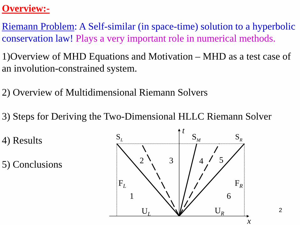
Overview:-

Riemann Problem: A Self-similar (in space-time) solution to a hyperbolic conservation law! Plays a very important role in numerical methods.

1)Overview of MHD Equations and Motivation – MHD as a test case of an involution-constrained system. 2) Overview of Multidimensional Riemann Solvers 3) Steps for Deriving the Two-Dimensional HLLC Riemann Solver 4) Results 5) Conclusions

t

x

1 6

3 4 5 2

SRSL SM

UL UR

FL FR

3

( ) ( )

( )( )

x2 2 2x x

x

x y x yy

x z x zz

2x x

x

y x y y x

zz x x z

v v + P + /8 B /4 v

v v B B /4 v v v B B /4 v

+ +P+ /8 v B /4t x0B

B v B v BB v B v B

− − − ∂ ∂ − ⋅ ∂ ∂ − − −

B

B v B

ρρρ π πρ

ρ πρρ πρ

π πεε

( ) ( )( )

( )

y z

x y x y x z x z2 2 2y y y z y z

y z y z z2

y y

x y y x

y z z y

v v v v B B /4 v v B B /4

v + P + /8 B /4 v v B B /4 v v B B /4 v

+ + +P+ /8 v B /4y zv B v B

0

v B v B

− − − −

− ∂ ∂ − ⋅∂ ∂ − − −

B

B v B

ρ ρρ π ρ π

ρ π π ρ πρ π ρ

π πε ( ) ( )( )( )

2 2 2z

2z z

z x x z

y z z y

+ P + /8 B /4 = 0+P+ /8 v B /4

v B v B

v B v B

0

− − ⋅ − − −

B

B v B

π π

π πε

−Ez

Ez

Ey

−Ey

−Ex Ex

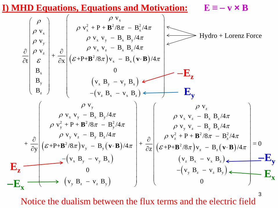
I) MHD Equations, Equations and Motivation: E ≡ − v × B

Notice the dualism between the flux terms and the electric field

Hydro + Lorenz Force

MHD Is Different:

Necessitates use of Yee-type mesh. Fluid variables still zone-centered. Magnetic fields at zone faces; electric fields at zone edges. Since B is defined on faces, we need a reconstruction of B over the zone that respects the constraint: Electric fields at edges require genuinely multi-d treatment – Need for at least genuinely 2D Riemann Solvers

1 + c = 0 ; ; constraint 0t c

∂∇× ≡ − × ∇ =

∂B E E v B B

4

0!∇ =BBx, i+1/2, j, k

Ey, i+1/2,j,k-1/2

x

y z

∆z

Ex, i,j-1.2,k-1/2

∆x

∆y

By, i,j-1/2,k E z, i

-1/2

,j-1/

2,k

Bz, i,j,k+1/2

Zone center i,j,k

There is a dualism between the fluxes of the conservation law and the electric field (Balsara & Spicer 1999). That can be exploited to obtain the electric field. For this concept to truly work, the electric field should be treated truly multidimensionally. All prior work had tried combinations of 1D RP to introduce multidimensionality into the electric field evaluation. There was even an attempt to stabilize the electric field by doubling the dissipation (Gardiner & Stone 2005). Why double? Why not 3, 4 or 5.5? Any doubling of dissipation proves to be completely unnecessary when the genuinely 2D HLL and HLLC Riemann solvers are used to obtain the edge-centered electric field (Balsara 2010, 2012). Essential ideas: Dualism of fluxes and E-field+ true multidimensional RS + Div-Free Reconstruction

5

II) Overview of Multidimensional Riemann Solvers

All Riemann problems (RP) are self-similar solutions of a hyperbolic conservation law. Often shown as a space-time diagram, see below. A one-dimensional RP arises in computer codes when two constant states come together at a zone boundary. Example for Euler equations shown below : 1– left state; 6– right state; 2– left-going rarefaction; 5– right-going rarefaction; 3&4 – states that separate the contact discontinuity. t

x

1 6

3 4 5 2

SRSL SM

UL UR

FL FR

6

Many of the details produced by a Riemann solver (RS) are never used in a computer code. Motivates need for an approximate Riemann solver – topic of this talk. See fig. below. The approximate RS has to satisfy some requirements: 1) A self-similar wave model in space-time. 2) Consistency with the conservation law, . 3) Entropy enforcement. Provide dissipation at rarefaction fans. 4) V. Desirable but not necessary: Preservation of internal sub-structures.

t

x

1 6

3 4 5 2

SRSL SM

UL UR

FL FR

t

x

SRSL T

SRTSLT

UL UR

FL FR

A

B C

D E

F *U ,F∗

Exact Riemann Solver Approximate HLL Riemann Solver 7

0t x∂ + ∂ =U F

Previous slides only described the 1d situation. Obtaining the strongly-interacting subsonic state U*, and associated flux F*, was of interest there.

It is desirable to introduce multi-dimensional effects in order to get more consistency with the physics. When 4 states come together at a vertex; we have a multi-dimensional RP. Two space + 1 time dimension.

Same principles used in more sophisticated way. Papers: Balsara (2010, 2012) JCP

t

x

SRSL T

SRTSLT

UL UR

FL FR

A

B C

D E

F *U ,F∗

x

y

t

* * *, ,U F G

R D Q

A

M

DRSD

LS *DU

C N B

o

1D HLL RS: 1 space + 1 time 2D HLL RS: 2 space + 1 time 8

The 1D and 2D HLL Riemann solvers, shown previously, average over important internal sub-structures in the RP. Specifically, the contact discontinuity is smeared.

The HLLC Riemann solver is an approximate RS that restores the contact discontinuity back into the Riemann problem. See below.

(For a thorough discussion of exact and approximate Riemann solvers, pl. see my upcoming textbook.)

t

x

1 6

3 4 5 2

SRSL SM

UL UR

FL FR

Exact Riemann Solver Approximate HLLC Riemann Solver

t

x

SRSL T

SRTSLT

UL UR

FL FR

A

B C

D E

F UR

∗

SM

UL∗

9

t

x

SRSL T

SRTSLT

UL UR

FL FR

A

B C

D E

F UR

∗

SM

UL∗

x

y

t

*1CU

R D Q

A

M

DRSD

LS*D+U

DMS

*2CU

C N B

o

K

J

1D HLLC RS 2D HLLC RS

Restoring the contact discontinuity in multi-dimensions is highly desirable. It permits flow structures to propagate isotropically in all directions relative to the mesh. CD moves at any angle w.r.t. mesh. The construction is more difficult, especially for the subsonic case, but it is described in detail in this paper. Supersonic cases are easy.

10

*D−U

Results:-

2D HLL and HLLC RS for any hyperbolic system of conservation laws.

The multi-d RS is implemented on a structured mesh at edges/vertices. Takes four input states and produces one output state and two output numerical fluxes.

Demonstrated successful implementation for Euler and MHD flows.

Works on structured meshes (Pl. ask me about movies!): – D.S. Balsara , J. Comp. Phys. 229, 1970-1993 (2010) D.S. Balsara, J. Comp. Phys., 231 (2012) 7476-7503 ( Please see http://www.sciencedirect.com/science/article/pii/S0021999111007467 )

Also works on unstructured meshes – Balsara, Dumbser & Abgrall (2013) More At: http://physics.nd.edu/people/faculty/dinshaw-balsara Please also see the website for my book: http://www.nd.edu/~dbalsara/Numerical-PDE-Course

11

12

Advantages:- The multi-dimensional RS is shown to work well even in 3D codes. Permits larger CFL to be used – in 2D and 3D. Cost-competitive with 1D RS technology. Flow features show greater isotropy in multi-dimensional flows. Electric field calculation in MHD does not require doubling of dissipation. Isotropic field propagation also helps with pressure positivity. This is especially true for low beta plasmas. Shown to work on a large number of stringent Euler & MHD problems.

13

III) Steps for Deriving the Two-Dimensional HLLC Riemann Solver Two-Rimensional Riemann Problems have been explored (using 1D RS technology) by Shulz-Rinne et al (1993).

They arise when four constant states come together at a corner. See the four states URU , ULU , ULD and URD and their evolution in time-sequence:

x

y

URU ULU

ULD URD

14 14

III) Steps for Deriving the Two-Dimensional HLLC Riemann Solver Two-Rimensional Riemann Problems have been explored (using 1D RS technology) by Shulz-Rinne et al (1993).

They arise when four constant states come together at a corner. See the four states URU , ULU , ULD and URD and their evolution in time-sequence:

15

x

y

SRTSLT

SUT

SDT

Q

A

MCN

O

R

B

D

RUULUU

LDU

RUF

RUG

LUF

LUG

RDF

RDG

LDF

LDGRDU

self-similar region of strong-interaction

RUULUU

LDURDU

Initial conditions: 2D RP; four input states Example 2D RP

In a computer code: The 2D RP arises when four constant states come together at a corner between four zones. See the four states that come together at a vertex URU , ULU , ULD and URD in figs. below.

This results in four 1D RP along the principal directions coupled with a self-similar region of strong-interaction. In the strongly interacting region, complex flow structures evolve self-similarly. See right figure for example.

For designing the 2D HLL RS, we take our cue from the 1D HLL RS. The constant state U* now becomes the region of strong interaction U*.

The introduction of the subsonic constant state U*, whether in 1D or 2D, provides the requisite dissipation as well as entropy enforcement.

Because of self-similarity, the constant state U* forms an inverted rectangular pyramid in a 3D space-time. Used to consistently obtain U* , F* , G* as outputs.

t

x

SRSL T

SRTSLT

UL UR

FL FR

A

B C

D E

F *U ,F∗

x

y

t

* * *, ,U F G

R D Q

A

M

DRSD

LS *DU

C N B

o

1D HLL RS (inverted triangle) 2D HLL RS (inverted pyramid) 16

t

x

SRSL T

SRTSLT

UL UR

FL FR

A

B C

D E

F UR

∗

SM

UL∗

x

y

t

*1CU

R D Q

A

M

DRSD

LS*D+U

DMS

*2CU

C N B

o

K

J

1D HLLC RS 2D HLLC RS

For designing the 2D HLLC RS, we take or cue from the 1D HLLC RS (Toro, Spruce & Speares1994, Batten et al. 1997). The constant state now includes the sub-structure associated with contact discontinuities.

Notice that and are different states in the figure below. We still have an inverted rectangular pyramid in space-time due to self-similarity.

*1CU *

2CU

17

*D−U

Three Important Ideas go into the design process for 2d HLL RP; We add a Fourth for 2D HLLC RP:

1) Obtaining Extremal speeds: The constant state, whether in 1D or 2D, provides the requisite dissipation only if the maximal signal speeds are used in each principal direction of the mesh. Focus on SR , SL , SU and SD in the figure below.

1D RP between ULU & URU + 1D RP between ULD and URD SR & SL.

1D RP between URD & URU + 1D RP between ULD and ULU SU & SD.

x

y

SRTSLT

SUT

SDT

Q

A

MCN

O

R

B

D

RUULUU

LDU RDU

RUF

RUG

LUF

LUG

RDF

RDG

LDF

LDG18

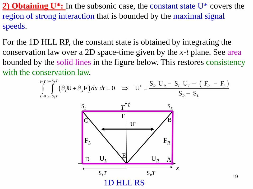
2) Obtaining U*: In the subsonic case, the constant state U* covers the region of strong interaction that is bounded by the maximal signal speeds.

For the 1D HLL RP, the constant state is obtained by integrating the conservation law over a 2D space-time given by the x-t plane. See area bounded by the solid lines in the figure below. This restores consistency with the conservation law.

t

x

SRSL T

SRTSLT

UL UR

FL FR

A

B C

D E

F U∗

1D HLL RS 19

( ) ( )0

S U S U F F 0 U

S S

R

L

x S Tt TR R L L R L

t xR Lt x S T

dx dt==

∗

= =

− − −∂ + ∂ = ⇒ =

−∫ ∫ U F

For the 2D HLL RP, consistency with the conservation law is obtained by integrating the conservation law over the 3D space-time in the x-y-t volume. See the volume bounded by the solid lines in figure below.

In the x=constant and y=constant side panels, the darkly shaded regions are the constant states from the 1D HLL RPs in the principal directions.

This provides consistency between the 2D RP and the 1D RP; I.e. the 2D RP will always default to the 1D RP when the variation in the flow is one-dimensional.

The pyramidal strongly-interacting state U* is contained within the rectangular Prism; only its base shows. That is adequate for giving us U* via space-time integration.

x

y

t

DRS

DLS

RDULDU

*DU

RUSR

DS

*RU

*U

R D Q

A

M

RUU

2D HLL RS 20

1D HLL RS

3) Obtaining F* & G*: In the subsonic case, the desired numerical flux F* associated with U* overlies the time axis. Thus an integration of the conservation law over a smaller domain in space-time that includes the time axis yields the numerical flux.

For the 1D HLL RP, the numerical flux is obtained by integrating the conservation law over a 2D space-time given by a part of the x-t plane. See area marked out by solid lines in the figure below. This restores consistency with the conservation law.

Supersonic cases are easier to treat by 1D upwinding.

21

( )

( )0 0

0

S F S F S S U UF =

S S

Rx S Tt T

t xt x

R L L R R L R L

R L

dx dt==

= =

∗

∂ + ∂ = ⇒

− + −−

∫ ∫ U F

t

x

SRSL T

SRTSLT

UL UR

FL FR

A

B C

D E

F U∗

*F

For the 2D HLL RP, consistency with the conservation law is obtained by integrating the conservation law over a sub-portion of the 3D space-time in the x-y-t volume. See the volume bounded by solid lines in figure below for the x-flux F* associated with U*.

The integration must include a plane that passes through the time axis.

In the x=constant and y=constant side panels, we have to integrate over sub-portions of the 1D HLL RPs in the principal directions. Integrals over side panels are quite intricate. Give us the numerical flux F* .

Supersonic cases are easier to treat by multidimensional upwinding.

2D HLL RS 22

x

y

t

DRS

DLS

RDULDU

*DU

RUSR

DS

*RU

*U

R D Q

A

M

RUU

*F

4) For obtaining the 2D HLLC RP, we need to slightly rethink the derivation of the 1D HLLC RP.

The conventional derivation focuses on the shock jumps at the right-going and left-going waves. The jump conditions at the contact are trivial.

However, realize that all space-time integrations should yield equivalent information. Consequently, the space-time integration of the conservation law over the area bounded by the solid line below should also yield the resolved state and flux for a 1D HLLC RP.

t

x

SRSL T

SRTSLT

UL UR

FL FR

A

B C

D E

F UR

∗

SM

UL∗

1D HLLC RS 23

x

y

t

*1CU

R D Q

A

M

DRSD

LS*D+U

DMS

*2CU

C N B

o

K

J

2D HLLC RS

x

y

SRTSLT

SUT

SDT

Q

A

MCN

O

R

B

D

*2CU

*1CU

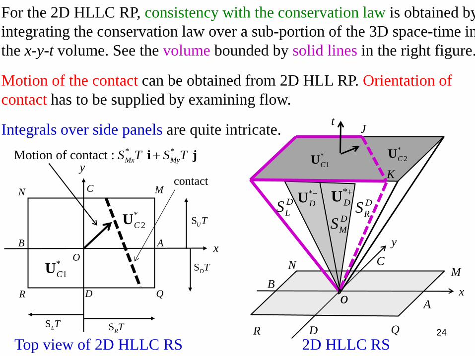
* *Motion of contact : Mx MyS T S T+i j

contact

Top view of 2D HLLC RS

For the 2D HLLC RP, consistency with the conservation law is obtained by integrating the conservation law over a sub-portion of the 3D space-time in the x-y-t volume. See the volume bounded by solid lines in the right figure.

Motion of the contact can be obtained from 2D HLL RP. Orientation of contact has to be supplied by examining flow.

Integrals over side panels are quite intricate.

24

*D−U

25

IV) Results

Accuracy analysis for multi-d RS presented in Balsara (2010) (2012) and Balsara, Dumbser & Abgrall (2013).

Test problems which emphasize advantages of multi-d approach are presented.

2D HLLC RS used in predictor and corrector steps. Alternatively, ADER is used in the predictor step with WENO reconstruction.

CFL numbers that are higher than those in conventional 2nd order Godunov schemes are used.

Hydro and MHD tests presented.

26

MHD Flow: Long term decay of Alfven Waves Run with CFL of 0.7. Alfven waves propagating very obliquely to mesh. The decay over long times is shown. Of all the choices shown, 2D HLLC RS with some amount of WENO technology shows the least dissipation.

Decay of Vz Decay of Bz

Time Time

Am

plitu

de

Am

plitu

de

27

MHD Flow: Magnetic Field Loop Advection Run with CFL of 0.9. Magnetic loop advected diagonally on a rectangular domain.

Conventional scheme doubles dissipation of the electric field (Gardiner & Stone 2005). The scheme with 2D HLLC RS does not double dissipation.

The propagation of the field loop is much more isotropic for 2D HLLC RS

Conventional 2nd order (Gardiner & Stone 2005): (CFL 0.45)

With 2D HLLC RS Balsara (2010, 2012): (CFL 0.9)

28

MHD Rotor Problem on ALE Mesh CFL 0.9; 80,000 elements ; ALE mesh

29

Accuracy for the MHD Vortex problem on an ALE Mesh Accuracy demonstrated from 1st to 5th order on 2D ALE Mesh.

30

MHD Flow: 3D MHD Blast with very low Plasma Beta Run with a CFL of 0.6. Near-infinite blast wave propagating through a magnetic plasma with β=0.001.

Accurate div-free propagation of B-field also gives better pressure positivity.

Density Pressure Velocity B-field magnitude

31

Relativistic MHD Riemann Problem with HLL and HLLC Riemann Solvers HLL HLLC

dens

ity

dens

ity

x x

32

V) Conclusions

1) Genuinely 2D HLL and HLLC RS presented. Input : multiple states in 2D. Output: 1 resolved state + 2 numerical fluxes.

2) Addressed all the issues with introducing a contact discontinuity. The speed and propagation direction of the contact is calculated by RS. Its original orientation has to be obtained by examining density gradient.

3) All the space-time integrals needed for the formulation are presented as explicit, computer-implementable, closed-form formulae. This makes the present RS technology very accessible.

4) The process of obtaining the numerical fluxes explicitly is presented.

5) Larger CFL numbers possible compared to conventional RS-based technology.

6) Predictor-Corrector like ADER-WENO formulation for any order, cost-competitive implementation is presented.

33

7) Much more isotropic propagation of flow features demonstrated for hydro and MHD flows. 8) There is no need to double dissipation when evaluating electric fields in MHD calculations. 9) The 2D HLLC RS also helps out with retaining pressure positivity in MHD problems with very low plasma-β. More At: http://physics.nd.edu/people/faculty/dinshaw-balsara Please also see the website for my book:

http://www.nd.edu/~dbalsara/Numerical-PDE-Course

Thanks for your attention!

34

Dinshaw S. Balsara (dbalsara@nd.edu) Univ. of Notre Dame

http://physics.nd.edu/people/faculty/dinshaw-balsara

http://www.nd.edu/~dbalsara/Numerical-PDE-Course