Multibrand geographic experiments

Art B. OwenGoogle Inc.

Tristan LaunayGoogle Inc.

October 2016

Abstract

In a geographic experiment to measure advertising e↵ectiveness, someregions (hereafter GEOs) get increased advertising while others do not.This paper looks at running B > 1 such experiments simultaneously on Bdi↵erent brands in G GEOs, and then using shrinkage methods to estimatereturns to advertising. There are important practical gains from doing this.Data from any one brand helps to estimate the return of all other brands.We see this in both a frequentist and Bayesian formulation. As a result,each individual experiment could be made smaller and less expensive whenthey are analyzed together. We also provide an experimental design formultibrand experiments where half of the brands have increased spend ineach GEO while half of the GEOs have increased spend for each brand. ForG > B the design is a two level factorial for each brand and simultaneouslya supersaturated design for the GEOs. Multiple simultaneous experimentsalso allow one to identify GEOs in which advertising is generally moree↵ective. That cannot be done in the single brand experiments we consider.

1 Introduction

It is di�cult to measure the impact of advertising even in the online settingwhere responses of individual users can be linked to conversion activities such asvisiting a website or buying a product. Regression models are often fit to suchrich observational data. While insights from observational data are suggestive,they seldom establish causal relations.

Google has expertise in using geographical experiments to measure the causalimpact of increased advertising, as decribed by Vaver and Koehler (2011, 2012).Advertising is increased in some regions and left constant or decreased in others(the control regions). Then the corresponding values of some key performanceindicator (KPI) are measured and related to the spending level. We will call theregions GEOs. The Nielsen company has designated market areas (DMAs) andtelevision market areas (TMAs). GEOs are similar but not necessarily identicalto these.

Other things being equal, it is easier to measure the impact of a large adver-tising change than a small one. Having two widely separated spend levels makes

1

arX

iv:su

bmit/

1740

411

[sta

t.ME]

1 D

ec 2

016

for a more informative experimental design. There are however practical and or-ganizational constraints on the size of an experimental intervention. Advertisingmanagers may be reluctant to experiment with large spend changes. Also, in asmall GEO, there may not be enough inventory of ad impressions to sustain alarge spending increase.

Both of these problems can be mitigated by experimenting on several brandsat once. The experimental design is like the one sketched below.

GEO 1 GEO 2 GEO 3 GEO 4 · · · GEO GBrand 1 + � + � · · · +Brand 2 � � + + · · · �

......

......

.... . .

...Brand B � + � + · · · +

Here the experiment gives Brand 1 an increased spending level in GEOs 1 and 3and the control level of spending in GEOs 2 and 4. Every brand gets increasedspend in half of the GEOs, with each GEO being in the test group for somebrands and the control group for others. The combined information from all Bbrands can then be used to get a good measure of the overall e↵ectiveness ofadvertising. Using shrinkage methods it is also possible for the data from onebrand to improve estimation for another one. Because the multibrand experimentpools information, it can be run with smaller spending changes than we wouldneed in single brand experiments.

An outline of this note is as follows. Section 2 presents regression models forsingle brands and multiple brands. Section 3 gives a scrambled checkerboardexperimental design in which half of the GEOs are treatment for each brandand half of the brands get the treatment level in each GEO. Subject to theseconstraints, there may be weak correlations among pairs of brands or amongpairs of GEOs. Section 3 also shows that certain classical designs (balancedincomplete blocks and Hadamard matrices) that might seem appropriate are,in fact, not well suited to this problem. Section 4 simulates a single brandexperiment 1000 times over 20 GEOs. The true return to advertising in thosesimulations is � = 5. There is reasonable power to detect � 6= 0 when advertisingis increased by 1% of prior period sales, but not when it is increased by only0.5% of prior sales. In either case the standard error of the estimated return isquite large. Section 5 describes a multibrand simulation with 30 brands in 20GEOs. The advertising return for brand b is �

b

⇠ N (5, 1). The estimator of Xieet al. (2012) that shrinks each brand’s parameter estimate towards their commonaverage is about 3.2 times as e�cient at estimating �

b

than using only thatbrand’s data, when the treatment is 1% of sales. For smaller treatments, 0.5% ofsales, shrinkage is about 7.8 times as e�cient as single brand experiments. Somesimulation details are placed in Section 6. Section 7 simulates a fully Bayesiananalysis. The simulation there has G = 160 GEOs but only B = 4 brands andit also shows a strong benefit from pooling. The Bayesian method has similaraccuracy to Stein shrinkage and comes with easily computed posterior credibleintervals. Section 8 has some conclusions and discussion.

2

2 Single- and multi-brand models

We target an experiment comparing an 8 week background period followed bya 4 week experimental period. To prepare for this project, data from 5 verydi↵erent advertisers was investigated. The industries represented were: hair care,cosmetics, outdoor clothing, photography and baked goods. There were strongsimilarities in the data for all of these industries.

If one plots the 8 week KPI for a brand versus the prior 4 week KPI for thatbrand, using one point per GEO the resulting points fall very close to a straightline on a log-log plot, in all 5 data sets. The linear pattern is so strong becausethe GEOs vary immensely in size.

Inspecting all of that data it became clear that the following model was agood description of a single brand’s data

Y post

g

= ↵0

+ ↵1

Y pre

g

+ �Xpost

g

+ "postg

, g = 1, . . . , G. (1)

Here Y post

g

is the KPI for GEO g in the experimental period, Y pre

g

is thecorresponding value in the pre-experimental period and Xpost

g

is the amountspent on advertising in GEO g in the post period. The basic linear regression ↵

0

+↵1

Y pre

g

is strongly predictive, because the underlying GEO sizes are very stableand the KPI is roughly proportional to size. There was not an appreciable weekto week autocorrelation for sales data within GEOs. What little autocorrelationthere was would be greatly diminished for multi-week aggregates such as an 8week prior period followed by a 4 week experimental one.

Model (1) is the one used by Vaver and Koehler (2011). The parameter ofgreatest interest is �. When Xpost

g

is the dollar amount spent on advertising,and the KPI Y post

g

is the revenue in the experimental period, then � is simplythe number of incremental dollars of revenue per dollar spent on advertising.The interpretability of � as a return to advertising is the reason why we workwith model (1). Modeling the logarithm of the KPI would have some statisticaladvantages, but it makes for a less directly interpretable �.

In simulations, the value of Xpost

g

is proportional to Y pre

g

. We take Xpost

g

=�Y pre

g

in the treatment group and Xpost

g

= 0 in the control group. Our defaultchoice is � = 0.01, representing di↵erential spend equal to one percent of priorsales. This need not mean setting advertising to 0 in the control group. HereXpost

g

is the level of additional spending above the historic or pre-planned levelfor that GEO. In an experiment that reduced spend in some GEOs to o↵setincreases in others, Xpost

g

would be negative in some GEOs and positive inothers.

In model (1), it is not reasonable to suppose that the errors "postg

are inde-pendent and identically distributed. In all five real data sets it was clear thatthe standard deviation of the KPI is larger for larger GEOs. To a very goodapproximation, the standard deviation was proportional to the KPI itself. Whensimulating model (1), Gamma random variables were used instead of Gaussianones. The standard deviation in a Gamma random variable is proportional toits mean. See Section 6.

3

Now suppose that a single advertiser has multiple brands b = 1, . . . , B. Itthen pays to experiment on all B brands at once. In a multibrand setting wecan fit the regression model

Y post

gb

= ↵0b

+ ↵1b

Y pre

gb

+ �b

Xpost

gb

+ "postgb

, b = 1, . . . , B, g = 1, . . . , G. (2)

The brands should be distinct enough that advertising for one of them doesnot a↵ect sales for another. For instance, two di↵erent diet sodas might be tooclosely related for this model to be appropriate.

The overall return to advertising is measured by

� =1

B

BX

b=1

�b

.

A combined experiment will be very informative about �. By using Steinshrinkage, the combined experiment can also give more accurate estimates ofindividual �

b

than we would get from just an experiment on brand b.

2.1 Di↵erential GEO responsiveness

A multibrand experiment can address some issues that are impossible to addressin a single brand experiment. Suppose for instance that advertising is moree↵ective in some GEOs than it is in others. In a single experiment an unusuallyresponsive or unresponsive GEO might generate an outlier, but we would notknow the reason. From a multibrand experiment we can fit the model

Y post

gb

= ↵0b

+ ↵1b

Y pre

gb

+ (�b

+ �g

)Xpost

gb

+ "postgb

. (3)

The new parameter �g

measures the extent to which advertising is especiallye↵ective in GEO g. In a single brand experiment with G responses we could notestimate these per-GEO parameters. It would amount to fitting 3+G regressionparameters to G responses. In a multibrand experiment we get G⇥B responsesand model (3) has only 3B +G regression parameters. If one consistently seesthat some GEOs have better responses to ads than others then it would bereasonable to focus more advertising in those GEOs. The parameter �

g

can stillbe practically important even when it is not large enough to generate outliers.

3 Scrambled checkerboard designs

For each brand, we should have half of the GEOs in the control group and halfin the treatment group. This necessitates an even number G of GEOs which isnot di�cult to arrange. Similarly, with an even number B of brands, each GEOshould be in the treatment group for half of the brands and in the control groupfor the other half. We would want to avoid a situation where a large GEO likeLos Angeles was the control group for most of the brands, or in the treatmentgroup for most of the brands.

4

A second order concern is that we would not want any pair of brands to alwaysbe treated together or in the control group together. For two brands the fourpossibilities {TT, TC,CT,CC} describe GEOs where the first brand is treatmentor control based on the first letter (T or C) and the second brand’s state isgiven by the second letter. Ideally we would like all four of these possibilities toarise equally often for all pairs of brands and an analogous condition to hold forGEOs.

This second order concern brings to mind balanced incomplete block (BIB)designs (Cochran and Cox, 1957), but that is a di↵erent concept and a BIBdoes not actually solve the problem. See Section 3.1. There is also potential forsubmatrices of Hadamard matrices to be good designs but that imposes unwantedrestrictions on the numbers B and G of brands and GEOs. See Section 3.2.

Theorem 1. Suppose that there are G � 1 GEOs and B � 1 brands where eachGEO has the treatment for half of the brands and each brand is in the treatmentgroup for half of the GEOs. Then it is impossible to have all four combinations{TT, TC,CT,CC} arise equally often for each distinct pair of GEOs as well asfor each distinct pair of brands.

Proof. If we represent our design by a G ⇥ B matrix Z of ±1s with +1 fortreatment and �1 for control, then each row and column of Z must sum tozero. The second order consideration about pairs TT through CC requires thecolumns of Z to be orthogonal. Since they are orthogonal to a column of 1sthere can only be G� 1 of them at most, so B G� 1. The same argumentapplied to rows yields G B � 1 We cannot have both G < B and B < G, so itis impossible to exactly satisfy the second order conditions.

Because the second order considerations cannot possibly be satisfied, wecompromise on them while still insisting on balance within every row and everycolumn.

A practical approach is to start with a G⇥B checkerboard pattern like thatin Figure 1, and randomly perturb it. Each brand gets the treatment in half ofthe GEOs and conversely each GEO is in the treatment group for half of thebrands. Then we use random swaps to break up the checkerboard pattern. Thesecond order criteria are then treated via random balance (Satterthwaite, 1959).

The swaps are based on a Markov chain studied by Diaconis and Gangolli(1995). Their setup uses 0s and 1s where we have ±1s, but results translatedirectly between the two encodings. We sample two distinct rows and twodistinct columns of the grid. If the pattern in the sampled 2 ⇥ 2 submatrixmatches ✓

+ ·· +

◆or

✓· ++ ·

◆

then we switch it to the other of these two. Here and below we use · in place of� where that would improve clarity. Diaconis and Gangolli (1995) show thatthis sampler yields a connected symmetric aperiodic Markov chain on the set ofbinary G⇥B matrices with row sums equal to B/2 and column sums equal toG/2. The stationary distribution is uniform on such matrices.

5

Multibrand design after 0 steps

Brand

GEO

Figure 1: A design where half of the 20 GEOs are treatment (black) for eachof the 30 brands and the others are control (white). Conversely, half of the30 brands are treatment group for each of the 20 GEOs and half are control.This design is unsuitable because any pair of brands either always get the sameallocation or always get an opposite allocation. We address that problem viascrambling.

Their setting was more general: the matrix contained nonnegative integerswith specified row and column sums, not just 0s and 1s. A verbatim translationof their algorithm would actually make the proposed switch with probability1/2. Raising the acceptance probability to 1 for binary matrices still satisfiesdetailed balance with respect to the uniform distribution, so the Markov chainstill uniformly samples the desired set of matrices.

Figure 2 shows the design after 100 attempts to flip a 4-tuple of elements.The original checkerboard pattern is still clearly visible and so 100 attempts arenot enough.

There are 16 possibilities for any 2⇥ 2 submatrix of the design and 2 of thesepossibilities are flippable. So we should expect that after the algorithm has beenrunning a while that the chance of a flip is about 1/8. The algorithm startswith a 100% flippable checkerboard and so it is reasonable to suppose that theflipping chance starts above 1/8 and decreases to that level. Each flip flips 4pixels in the image. Therefore we reverse about 1/2 pixels per attempt. Figure 3shows the result after 30,000 attempts so that the average number of flips perpixel is about 25.

6

Multibrand design after 100 steps

Brand

GEO

Figure 2: Design from Figure 1 after 100 attempted flips, showing that morethan 100 attempts are needed.

The algorithm is very fast. To do 90,000 steps on a larger 60⇥ 30 grid takesjust over 7 seconds in R on a commodity PC. It is possible to do many moreflips, but that seems unnecessary.

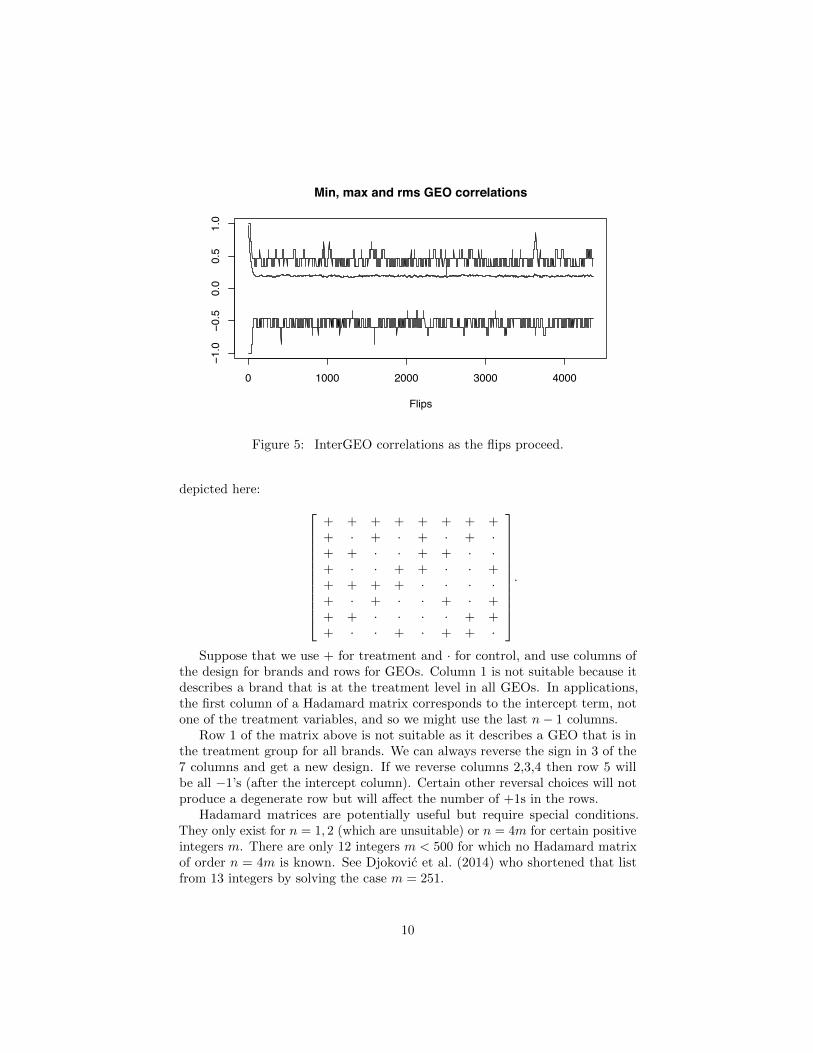
We can look at the correlations among brands as the sampling proceeds.There are B brands and hence B(B � 1)/2 di↵erent o↵-diagonal correlations.The minimum, maximum and root mean squared correlations among brandsare plotted in Figure 4. The same quantities for GEOs are plotted in Figure 5.These correlations are remarkably stable after a short warm-up period. Thestability has set in before BG/2 = 300 successful flips have been made.

There is a relationship among the sum of squared GEO correlations and thesum of squared brand correlations at every step of the algorithm. For brands b, b0

their correlation is ⇢bb

0 = (1/G)P

G

g=1

Xbg

Xb

0g

. For GEOs g, g0 their correlation

is ⇢gg

0 = (1/B)P

B

b=1

Xbg

Xbg

0 . Then counting cases g = g0 and b = b0,

X

gg

0

⇢2gg

0 =S

B2

, andX

bb

0

⇢2bb

0 =S

G2

, where

S =X

g

X

g

0

X

b

X

b

0

Xbg

Xb

0g

Xbg

0Xb

0g

0

7

Multibrand design after 30000 steps

Brand

GEO

Figure 3: Design from Figure 1 after 30,000 attempted flips.

which can be rearranged to get

X

b 6=b

0

⇢2bb

0 =B2

G2

X

g 6=g

0

⇢2gg

0 +1

G.

This phenomenon was noted by Efron (2008) in some work on doubly standardizedmatrices of microarray data. The mean squared correlation is comparable insize to what we would get with independent sampling. That is, we are able tobalance all GEOs and all brands exactly without paying a high cost on thesecorrelations.

The rest of this section considers classical designs that do not apply to oursituation and then considers when designs that meet our secondary goals can beconstructed. Some readers might prefer to skip to Section 4 which discusses asimulated example.

3.1 Designs derived from a BIB

In a BIB, one compares B quantities in blocks of size s < B and every pair ofquantities appears together in the same number of blocks. A BIB with blocksize s = B/2 and one block per GEO might be repurposed for multi-brandexperiments by making the B/2 elements of each block correspond to brandsgiven the treatment level. A small example with B = 4 brands and G = 6 GEOs

8

0 1000 2000 3000 4000

−1.0

−0.5

0.0

0.5

1.0

Min, max and rms brand correlations

Flips

Figure 4: Interbrand correlations as the number of successful flips increases.

looks like this

2

6666664

B1 B2 B3 B4

G1 + + · ·G2 + · + ·G3 + · · +G4 · + + ·G5 · + · +G6 · · + +

3

7777775

where a + indicates that the given brand gets the treatment in the given GEO.The problem is that GEOs 1 and 6 are exact opposites as are GEOs 2 and 5 andGEOs 3 and 4. Similarly, for any pair of brands the matrix

+ ·

+ 1 2· 2 1

�

gives the number of GEOs at each treatment combination. We know fromTheorem 1 that equal numbers in all four configurations cannot be attained.Here we see that for this BIB any two brands are more likely to be at oppositetreatment versus control settings than at the same level.

3.2 Designs derived from a Hadamard matrix

A Hadamard matrix (Hedayat et al., 2012) H is an n⇥ n matrix with elements±1 satisfying HTH = HHT = I

n

. An example Hadamard matrix with n = 8 is

9

0 1000 2000 3000 4000

−1.0

−0.5

0.0

0.5

1.0

Min, max and rms GEO correlations

Flips

Figure 5: InterGEO correlations as the flips proceed.

depicted here:

2

66666666664

+ + + + + + + ++ · + · + · + ·+ + · · + + · ·+ · · + + · · ++ + + + · · · ·+ · + · · + · ++ + · · · · + ++ · · + · + + ·

3

77777777775

.

Suppose that we use + for treatment and · for control, and use columns ofthe design for brands and rows for GEOs. Column 1 is not suitable because itdescribes a brand that is at the treatment level in all GEOs. In applications,the first column of a Hadamard matrix corresponds to the intercept term, notone of the treatment variables, and so we might use the last n� 1 columns.

Row 1 of the matrix above is not suitable as it describes a GEO that is inthe treatment group for all brands. We can always reverse the sign in 3 of the7 columns and get a new design. If we reverse columns 2,3,4 then row 5 willbe all �1’s (after the intercept column). Certain other reversal choices will notproduce a degenerate row but will a↵ect the number of +1s in the rows.

Hadamard matrices are potentially useful but require special conditions.They only exist for n = 1, 2 (which are unsuitable) or n = 4m for certain positiveintegers m. There are only 12 integers m < 500 for which no Hadamard matrixof order n = 4m is known. See Djokovic et al. (2014) who shortened that listfrom 13 integers by solving the case m = 251.

10

A more serious problem is that dropping the first column of a Hadamardmatrix and toggling the signs of some columns is only useful if B�1 = G = 4m forsome m. One could drop the first row too, yielding a design for B = G = 4m� 1which has near balance for each brand and each GEO. But both of these choicesimpose unwanted restrictions on B and G. In principal one could take a G⇥Bsubmatrix of the last n� 1 rows and columns of a Hadamard matrix but thenthe result is even farther from the desired balance of having each brand get thecontrol treatment in G/2 GEOs and each GEO delivering the control treatmentto each of B/2 brands.

3.3 Constraints

When B � 2 and G � 2 are both even then the design matrix we want is B ⇥Gbinary matrix with B/2 ones in each column and G/2 ones in each row. Suchmatrices always exist. We would also like, when possible, to have no two rowsor columns be identical, or to be opposite of each other.

Definition 1. Two vectors v1

, v2

2 {�1, 1}k have a collision if either v1

= v2

or v1

= �v2

. A matrix X 2 {�1, 1}n⇥p has no collisions if no two of its rowshave a collision and no two of its columns has a collision.

Definition 2. A matrix X 2 {�1, 1}n⇥p is balanced if each row sums to 0 andeach column sums to 0.

Our design uses balanced binary matrices. Ideally we would like our designmatrix to be free of collisions. This secondary constraint cannot always be met.For any even number B there are only

�B

B/2

�di↵erent binary vectors having

exactly B/2 ones. Because we don’t want duplicates or opposite pairs we musthave G

�B

B/2

�/2, and conversely B

�G

G/2

�/2.

First, if B = 2 then any pair of GEOs must get either the exact sameor exact opposite treatment, and similarly for brands when G = 2. So whenmin(B,G) = 2 collisions will occur.

Theorem 2. Let B � 2 and G � 2 be even numbers. If min(B,G) 4 thenthere is no balanced binary G⇥ B matrix without collisions. If B = G = 6 orB = G = 8, then there is such a matrix.

Proof. If G = 2 then the result is obvious because the second row must thenbe the opposite of the first one. Similarly if B = 2, and so no such matrix isavailable when min(B,G) = 2.

For G = B = 4, consider a 4 ⇥ 4 matrix of + and · with exactly two +symbols in each row and each column. We can sort the columns so that thefirst row is

�+ + · ·

�. If the matrix has no collisions, then each subsequent

row must have exactly one + in the first two columns and one + in the last twocolumns. Because each column has two +’s, only one of the next three rows canhave a + in column 1 and only one of those rows can have a + in column 2.There is therefore no way to put three more rows into the matrix without havinga collision. As a result there is no collision free balanced 4⇥ 4 matrix. There

11

cannot be a collision free balanced binary G⇥4 matrix with G � 6 either. Thereare only

�4

2

�= 6 distinct such rows and using them all would bring collisions.

Similarly, there are no B ⇥ 4 collision free balanced binary matrices.When B = G = 6, it is possible to avoid collisions. For instance, we could

use the matrix0

BBBBBB@

+ + + · · ·+ + · + · ·+ · · · + +· + · · + +· · + + + ·· · + + · +

1

CCCCCCA, (4)

which has no collisions. For B = G = 8 we could use0

BBBBBBBBBB@

+ + + + · · · ·+ + · · · · + ++ · + · + + · ·+ · · + · + + ·· + + + + · · ·· + · · + + · +· · + · + · + +· · · + · + + +

1

CCCCCCCCCCA

. (5)

The first three columns of the matrix in (5) are the same as in a classical 23

factorial design. That matrix is not such a design, and indeed that design wouldnot have balanced rows.

Next we consider how to create larger G⇥B balanced binary collision freematrices from smaller ones.

Theorem 3. Let X 2 {�1, 1}B⇥G be a balanced binary matrix with no colli-sions. Then there is a balanced binary matrix X 2 {�1, 1}(B+4)⇥(G+4) with nocollisions.

Proof. Let r1

and r2

be the first two rows of X, let c1

and c2

be the first twocolumns of X and choose z 2 {�1, 1}. Now let

X⇤ =

0

BBBB@

X c1

�c1

c2

�c2

r1

z z �z �z�r

1

z z �z �zr2

�z �z z z�r

2

�z �z z z

1

CCCCA. (6)

Every row and every column of X⇤ is balanced by construction. There are nocollisions among the first B rows or first G columns of X⇤ because there arenone in X.

12

Now we consider the last four rows of X⇤. Row B + 1 does not collide withthe last two rows because r

1

does not collide with r2

. Rows B +1 and B +2 areopposite in their first G columns but they agree in the next 4 columns so theydo not collide. By symmetry, this argument shows that there are no collisionsamong the last four rows of X⇤ or among the last four columns.

It remains to check whether any of the new rows (or columns) collide withany of the old ones. Row B + 1 of X⇤ cannot collide with row k of X⇤ for any1 < k B because r

1

does not collide with any of the corresponding rows of X.Rows B + 1 and 1 of X⇤ agree in the first G columns but di↵er in exactly twoof the last 4 columns of X⇤ so they do not collide. Therefore row B + 1 of X⇤

does not collide with any of the first B rows. Row B + 2 of X⇤ equals r1

in itsfirst G columns. Therefore it cannot collide with row k of X⇤ for any 1 < k B.By construction it matches row 1 in two of the new columns and is opposite row1 in the other two. It follows that none of the last four rows of X⇤ collide withany of the first B rows. By symmetry there are no collisions among any of thelast four columns of X⇤ and any of the first G columns.

The Theorem above gives an approach to creating design matrices. We startwith a small matrix and grow it by repeatedly applying equation (6). It is notnecessary to grow X via the first two rows and columns. It would work to chooseany two distinct rows or columns. For instance they could be chosen randomlyor chosen greedily to optimize some property of the resulting matrix.

Repeatedly applying equation (6) will give a nearly square matrix becauseit keeps adding 4 to both the number of rows and the number of columns. Wemight want to have G � B.

We can grow the matrix by 4 rows and 8 columns via

X⇤ =

0

BBBB@

X c1

�c1

c2

�c2

c3

�c3

c4

�c4

r1

z1

z1

�z1

�z1

z2

z2

�z2

�z2

�r1

z1

z1

�z1

�z1

z2

z2

�z2

�z2

r2

�z1

�z1

z1

z1

�z2

�z2

z2

z2

�r2

�z1

�z1

z1

z1

�z2

�z2

z2

z2

1

CCCCA, (7)

for any z1

, z2

2 {�1, 1} where r1

and r2

are any two rows of X and c1

, . . . , c4

are any four columns of X. Equation (7) adds four rows and eight columns. Thesame idea could extend a G⇥B matrix to a 3G⇥ (B + 4) matrix, tripling thenumber of columns (GEOs) while adding only four rows (brands).

The methods of this section show that there are some large collision freedesigns. We find that starting with the matrix (4) or (5) and growing it byrepeatedly applying (6) yields designs that include some correlations very close to±1. The scrambled checkerboard approach tends to produce designs with smallermaximum absolute correlation than the growth approach. Also, numericallysearching with that algorithm turns up 8⇥8 designs but not 6⇥8 designs, whichwe suspect do not exist.

13

●

●

●

●

●

●

●

●

●

●

●

●

●

●

●

●

●

●

● ●

2e+06 4e+06 6e+06 8e+06

1e+0

62e

+06

4e+0

6

KPI

Prior period (8 weeks)

Test

per

iod

(4 w

eeks

)

Figure 6: One realization of a single brand simulation. Treatment GEOs are inred, control in black. The reference line is at y = x/2 because the test periodhas half the length of the prior period.

4 Regression results

The regression model (1) was simulated with advertising e↵ectiveness � = 5.0in 20 GEOs of which 10 had increased spend equal to 1% of the prior period’ssales. Further details are in Section 6. Figure 6 shows one realization. Thesimulation was done 1000 times in total. Then, using the same random seeds,the simulation was repeated with increased spend of 0.5% instead of 1%.

For each simulated data set, weighted least squares regression was used. Theweights were proportional to (1/Y pre)2, making them inversely proportional tovariance. Unweighted regression does not give reliable confidence intervals andp-values in this setting.

Some results are plotted in Figure 7 and some numerical summaries are inTable 1. The top panels of Figure 7 show histograms of 1000 two-sided p-valuesfor H

0

:� = 0. This null was rejected 28.6% of the time for the experiment with asmaller treatment size, and 81.3% of the time for the one with a larger treatmentsize. The middle panels show histograms of twice the standard error of �, roughlythe distance from � to the edge of a 95% confidence interval. At 0.5% treatmentthis uncertainty averaged 6.68 while at 1% it averaged 3.34, just over 66% of thetrue value 5. The root mean squared error in � was 3.21 for small treatmentdi↵erences and 1.61 for large ones. The bottom panels show histograms of theestimates � for only those simulations in which H

0

was rejected at the 5% level.The average estimated e↵ect was 8.64 for the smaller treatment size and 5.51 forthe larger one.

The smaller treatment size has very low power, very wide confidence intervals,

14

Extra spend 0.5%

WLS p val for advertising

Freq

uenc

y

0.0 0.2 0.4 0.6 0.8 1.0

050

100

150

Extra spend 1.0%

WLS p val for advertising

Freq

uenc

y

0.0 0.2 0.4 0.6 0.8

020

040

060

0

Extra spend 0.5%

Two s.e.s

Freq

uenc

y

4 6 8 10

020

4060

80

Extra spend 1.0%

Two s.e.s

Freq

uenc

y

2 3 4 50

2040

6080

Extra spend 0.5%

Estimates given significance

Freq

uenc

y

4 6 8 10 12 14 16

05

1015

20

●

Extra spend 1.0%

Estimates given significance

Freq

uenc

y

4 6 8 10

020

40

●

Figure 7: Results from repeated single brand simulations.

and in those instances where it detects an advertising e↵ect, it gives a substantialoverestimate of e↵ectiveness. The larger treatment size has greater power andonly slight overestimation of � when it is significant. But it still yields a wideconfidence interval for �.

5 Multibrand experimental results

The multibrand setting was simulated with B = 30 brands over G = 20 GEOs.Treatment versus control was assigned with scrambled checker designs fromSection 3. The e↵ectiveness of brand b was generated from �

b

⇠ N (5, 1), soadvertising returns are usually in the range from 3 to 7.

15

Trt cPr(p 0.05) 2se(�) E((� � �)2)1/2 E(� | p 0.05)

0.5% 0.29 6.68 3.21 8.641.0% 0.81 3.34 1.61 5.51

Table 1: Output summary of 1000 simulations of the single brand experiment.

5.1 Shrinkage estimation of �b

We write �b

for the least squares estimate of �b

from brand b data and setˆ� = (1/B)

PB

b=1

�b

. We can estimate �b

by a shrinkage estimator formed as a

weighted average of �b

and ˆ�. Xie et al. (2012, Section 4) propose estimators ofthe form

�b

=�

var(�b

) + ��b

+var(�

b

)

var(�b

) + �ˆ� (8)

for a parameter � that must be chosen. The larger � is, the more emphasis weput on brand b’s own data instead of the pooled data. For brands with large

var(�b

), more weight is put on the pooled estimate ˆ�. Xie et al.’s (2012) maininnovation is in shrinkage methods for data of unequal variances as we have here.To use their method we replace var(�

b

) by unbiased estimates cvar(�b

) takenfrom the linear model output, and choose �.

Xie et al. (2012) give theoretical support for choosing � to minimize thefollowing unbiased estimate of the expected sum of squared errors

SUREG(�) =1

B

BX

b=1

var(�b

)2

(var(�b

) + �)2(�

b

� ˆ�)2

+1

B

BX

b=1

var(�b

)

var(�b

) + �

⇣�� var(�

b

) +2

Bvar(�

b

)⌘.

(9)

This function is not convex in � but a practical way to choose � is to evaluateSUREG on a grid of, say 1001, � values. Letting the typical weight on �

b

takevalues u 2 {0, 1/1000, 2/1000, . . . , 1} we use

� =1

B

BX

b=1

var(�b

)⇥ u

1� u

where u = 1 means � = 1 which simply means �b

= �b

.We can measure the e�ciency gain from shrinkage via

E↵ =1

B

PB

b=1

(�b

� �b

)2

1

B

PB

b=1

(�b

� �b

)2.

Figure 8 shows a histogram of this e�ciency measure in 1000 simulations. Onaverage it was about 3.17 times as e�cient to use shrinkage when the experimental

16

Relative efficiency of pooling

MSE( indiv ) / MSE( shrunk )

Freq

uenc

y

0 2 4 6 8

050

150

●

(a) Experimental spend 1%.

Relative efficiency of pooling

MSE( indiv ) / MSE( shrunk )

Freq

uenc

y

0 5 10 15 20

050

100

150

●

(b) Experimental spend 0.5%.

Figure 8: Relative e�ciency of shrinkage estimates compared to single brandregressions.

treatment is to increase advertising by 1% of prior sales. For smaller experiments,at 0.5% of sales, the average e�ciency gain was 7.82. For each given brandb, the information from B � 1 other brands’ data yields a big improvement in

accuracy. Recall that �b

iid⇠ N (5, 1). The gain from shrinkage would be less ifthe underlying �

b

were less similar and greater if they were more similar.

5.2 Average return to advertising

The quantity � measures the overall return to advertising averaged over allbrands. Although individual returns �

b

are more informative, their average canbe estimated much more reliably. In small experiments where some individual

�b

’s are not well determined it may be wiser to base decisions on ˆ�.

We can estimate � by ˆ� = (1/B)P

B

b=1

�b

and then using the individual

regressions compute cvar( ˆ�) = B�2

PB

b=1

cvar(�b

). Figure 9 shows histograms of

2(cvar( ˆ�))1/2. Table 2 compares average values of twice the standard error for �

in a single brand experiment with twice the standard error for ˆ� in a multibrandexperiment. As we might expect the multibrand standard errors are roughlypB =

p30 times smaller. Similarly, doubling the spend roughly halves the

standard error.

6 Simulation details

In each simulation, the design was generated by the scrambled checker algo-rithm described in Section 3. Then the data were sampled from the Gammadistributions described here.

17

Global return accuracy

2 standard errors

Freq

uenc

y

0.55 0.60 0.65 0.70

040

80

●

(a) Experimental spend 1%.

Global return accuracy

2 standard errors

Freq

uenc

y

1.10 1.20 1.30 1.40

020

4060

●

(b) Experimental spend 0.5%.

Figure 9: Two standard errors of ˆ�.

1% spend 0.5% spend

Single Multiple Single Multiple

3.34 0.62 6.68 1.23

Table 2: Average over simulations of two standard errors for � (single brands)

and ˆ� (multiple brands).

6.1 Gamma distributions

The Gamma distribution has a standard deviation proportional to its mean,matching a pattern in the real sales data. When the shape parameter is > 0the Gamma probability density function is x�1e�x/�() for x > 0. To specifya scale parameter, we multiply X ⇠ Gam() by the desired scale ✓.

The random variable ✓X has mean ✓ and variance ✓2, leading to a coe�cientof variation equal to 1/

p for any ✓. The shape = 1/cv2 yields a Gamma

random variable with the desired coe�cient of variation.The coe�cient of variation for the average of n observations from one GEO

(e.g., npost

= 4 in the test period and npre

= 8 in the background period) isapproximately 1/

pn times the coe�cient of variation of a single observation.

The coe�cient of variation for single observations from a set of 8 week trialperiods was about 0.15 while that for 4 week followup periods was about 0.1.These figures are based on aggregates over GEOs that were very similar for allof the di↵erent brands. An 8 week trial period has within it more seasonalitythan a 4 week period has, and so it is reasonable that we would then measure alarger coe�cient of variation.

To simulate with a specific coe�cient of variation we use = n/cv2. This

18

leads to pre

= 8/0.152.= 356 and

post

= 4/0.12 = 400.Gamma random variables are never negative which gives them a further

advantage over simulations with Gaussian random variables. For the specificparameter choices above, the shape parameters are large enough that the Gammarandom variables are not strongly skewed (their skewness is 2/

p). A Gaussian

distribution might give similar results. The Gamma distribution is useful becauseit can be used to simulate either strongly or mildly skewed data that are alwaysnonnegative.

6.2 Data generation

For a single brand experiment, the data are generated as follows. First theunderlying sizes of the GEOs were sampled as S

g

= 107�Ug where Ug

⇠ U(0,�),for g = 1, . . . , G. The quantity S

g

is interpreted as a size measure for GEO g.We will use it as the expected prior sales, which is then roughly proportional tothe number of customers in GEO g. Choosing � = 1 means that we considerGEOs ranging in size by a factor of about 10 from largest to smallest.

The prior KPIs are generated as

Y pre

g

ind⇠ Sg

⇥Gam(pre

)/pre

,

where pre

= npre

/cv2pre

. Then E(Y pre

g

) = Sg

. Let the spending level in theexperimental period be Xpost

g

in GEO g. Then the KPI in the experimentalperiod is generated as

Y post

g

ind⇠ npost

npre

⇥ Sg

⇥Gam(post

)/post

+Xpost

g

�,

where post

= npost

/cv2post

. The factor npost

/npre

adjusts for di↵erent sizes ofprior and experimental observation windows. The term Xpost

g

� is the additionalKPI attributable to advertising.

6.3 Checkerboard designs

The scrambled checkerboard design was run for 2⇥G⇥B ⇥ 25 = 30,000 steps.The expected number of flips for each pixel in the image is 25. This is muchmore than the number at which the root mean squared correlations stabilize.

7 A fully Bayesian approach

Stein shrinkage is an empirical Bayes approach. Here we consider a fully Bayesianalternative. When it comes to pooling information together from observationsthat arise from a common model but corresponding to di↵erent sets of parameters,Bayesian hierarchical models arise as a natural solution.

One advantage of the Bayesian approach is that it allows us to present theuncertainty in our estimates. For each brand b, we can get an interval (L

b

, Ub

)

19

such that Pr(Lb

�b

Ub

| data) = 0.95 without making any (additional)assumptions. These posterior credible intervals are easier to compute thanconfidence intervals from Stein shrinkage. We can also use posterior credibleintervals at the planning stage. To do that, we simulate the data several timesand record how wide the posterior credible intervals are. If they are too wide wemight add more GEOs or increase the di↵erential spend �.

7.1 A hierarchical model

We consider model (2) in a Bayesian context, which translates as follows:

µgb

:= ↵0b

+ ↵1b

Y pre

gb

+ �b

Xpost

gb

, b = 1, . . . , B, g = 1, . . . , G (10)

Y post

gb

⇠ N⇣µgb

,��b

/Y pre

gb

�2

⌘, b = 1, . . . , B, g = 1, . . . , G (11)

�2

b

⇠ IG(10�3, 10�3), b = 1, . . . , B (12)

�b

⇠ N (�,�2

�

), b = 1, . . . , B (13)

�2

�

⇠ IG(0.5, 0.5), and, (14)

� ⇠ 1R. (15)

Definitions (10), (11) and (12) the mirror model (2) that we described earlier.Notice that we signal the weighted regression explicitly in (11). The hierarchicalGaussian prior (13) on the coe�cients �

b

involves two new hyperparameters �and �2

�

which respectively represent the overall mean and variance of all returns�b

. Since we assumed in the beginning that all brands had somewhat similarreturns, we choose a semi-informative prior (14) on �2

�

that favors plausible, nottoo large, values. For our simulations we use a flat prior (15) on � relying on thedata to drive the inference. One could also use a Gaussian prior for �, craftingits mean and variance based on the prior knowledge of the brands at hand.

7.2 Simulation details

The data were generated according to the procedures described in Section 6.Samples were collected from the posterior distribution using STAN software(Stan Development Team, 2016).

We simulated many di↵erent conditions and consistently found that the Steinand Bayes estimates were close to each other. In this section we present justone simulation matching parameters of interest to some of our colleagues atGoogle. We consider G = 160 GEOs, only B = 4 brands and we take advertisinge↵ectiveness �

b

to be N (1, 1). Using E(�b

) = 1 produces a setting where adollar of advertising typically brings back a dollar of sales in the observationperiod. That implies a short term loss with an expected longer term benefitfrom adding or retaining customers. Taking the standard deviation of �

b

to oneimplies very large brand to brand variation. We still see a benefit from poolingonly 4 brands as diverse as that. The amount of extra spend is set to 1% ofprior sales (� = 0.01). We repeated this simulation 1000 times.

20

In this setting with 160 GEOs and 4 brands there will always be some GEOsthat get the exact same treatment for all 4 brands.

7.3 Agreement with shrinkage estimates

Figure 10 compares the RMSE [(1/B)P

B

b=1

(�b

� �b

)2]1/2 for Stein and Bayesestimation in 1000 simulations with B = 4. The methods have very similaraccuracy. For high brand to brand standard deviation �

b

= 1.0, there is a slightadvantage to Bayes. For lower brand to brand standard deviation �

b

= 0.25,there is a small advantage to Stein. The Bayesian estimate was at a disadvantagethere because the prior variance was 1/Gamma(0.5, 0.5) giving �

b

a median ofabout 1.48. This shows that the Bayesian estimate is not overly sensitive to ourwidely dispersed prior distribution on �

b

.

7.4 Posterior credible intervals

To investigate what power can be gained pooling data together using a multibrandexperiment over conducting multiple single-brand experiments independently, wesimulated datasets following the same procedure as before, using G = 160 GEOswith either B = 1 (no pooling) or B = 4 (pooling) brands, the e↵ectivenessesof which were drawn from a Gaussian distribution N (1,�2

b

) with �b

= 0.25.Now the brands return on average one dollar of incremental revenue per dollarspent, and the standard deviation of 0.25 represents substantial brand di↵erences.The relative incremental ad-spend we made varies from 0.5% to 2% to showhow it impacted the results. Figure 11 displays the estimated densities (over10,000 replications) of the half-width of 95% credible intervals around the brands’e↵ectivenesses, the solid lines representing the 95% quantile of these densities,in each scenario.

While the half-width of credible intervals does not quite display an inverserelationship with the extra spend when pooling multiple experiments together asit does when conducting experiments separately (doubling the incremental spendlets us detect twice as small an e↵ectiveness in the single-brand scenario), it isclear that pooling experiments together does bring improvement to the power ofthe geoexperiments.

It is best if posterior credible intervals have frequentist coverage levels closeto their nominal values. Table 3 shows empirical coverage levels for B = 4brands and G = 160 GEOS for a range of average returns � and brand to brandstandard deviations �

b

. On the whole the coverage is quite close to nominal.There is slight over coverage, probably due to the prior being dominated by largevalues of �

b

.

8 Conclusions and discussion

In our examples we see that combining data from multiple brands at once leadsto more accurate experiments than single brand experiments would yield. This

21

0.25

0.50

0.75

1.00

1.25

0.0 0.3 0.6 0.9 1.2bayes_local_err

stein_local_err

(a) Stein versus Bayes RMSE, �b = 1.

0

5

10

15

−0.2 −0.1 0.0 0.1 0.2 0.3diff_local_err

dens

ity

Diff of RMSEs (local): STEIN − BAYES

(b) Stein minus Bayes RMSE, �b = 1.

0.0

0.3

0.6

0.9

0.25 0.50 0.75 1.00bayes_local_err

stein_local_err

(c) Stein versus Bayes RMSE, �b = 0.25.

0

2

4

−0.3 −0.2 −0.1 0.0 0.1 0.2diff_local_err

dens

ityDiff of RMSEs (local): STEIN − BAYES

(d) Stein minus Bayes RMSE, �b = 0.25.

Figure 10: Comparison of Bayes and Stein RMSEs on two simulations of 1000replicates with B = 4 brands.

happens for both Bayes and empirical Bayes (Stein shrinkage) estimates. Theestimate for any given brand gets better by using data from the other brands.

This e�ciency brings practical benefits. An experiment on multiple brandsmight need to use fewer GEOs, or it might be informative at smaller, lessdisruptive, changes in the amount spent.

Ordinary Stein shrinkage towards a common mean is advantageous whenB � 4 by the theory of Stein estimation (Efron and Morris, 1973). The methodof Xie et al. (2012) is further optimized to handle unknown and unequal variances.

We have simply plugged in unbiased estimates of variance. Hwang et al.(2009) propose a di↵erent method that begins with shrinkage applied to thevariance estimates themselves. They also develop confidence intervals that could

22

0

10

20

0

10

20

0

10

20

extraSpend: 0.005extraSpend: 0.01

extraSpend: 0.02

1 2 3bayes_local_halfwidth

dens

ity

estimationnot−pooling

pooling

Half−width of cred. interval around (local) coef + quantile

Figure 11: Distribution of the half-width of credible intervals around brands’e↵ectiveness coe�cients.

�✏�b

0.10 0.25 0.50 0.75 1.00

0.25 0.974 0.974 0.967 0.953 0.9500.50 0.975 0.967 0.962 0.954 0.9460.75 0.974 0.968 0.967 0.959 0.9521.00 0.978 0.975 0.969 0.964 0.9541.25 0.975 0.968 0.966 0.960 0.9581.50 0.978 0.968 0.966 0.954 0.954

Table 3: Observed coverage levels of 95% Bayesian credible intervals. Six valuesof average gain � and five values of brand standard error �

b

.

be used for our �b

. Stein shrinkage is a form of empirical Bayes estimation. Wefound that by using a Bayesian hierarchical model we could get posterior credibleintervals with good frequentist coverage.

For planning purposes it is worthwhile to consider what parameter valuesare realistic in a specific setting. By simulating several choices we can find anexperiment size that gets the desired accuracy at acceptable cost.

The most di�cult quantity to choose for a simulation is �2

b

, the varianceof the true returns �

b

to advertising for di↵erent brands. That is di�cultbecause one often starts from a position of not having good causal values forany individual brand. One more values for this parameter must then be chosenbased on intuition or opinion. Because the true response rate to advertisingcan be expected to drift it is reasonable to suppose that multiple experimentswill need to be made in sequence. Estimates of �2

b

from one experiment will be

23

useful in planning the next ones.

Acknowledgments

Thanks to Jon Vaver, Jim Koehler, David Chan and Qingyuan Zhao for valuablecomments. Art Owen is a professor at Stanford University, but this work wasdone for Google Inc., and was not part of his Stanford responsibilities.

References

Cochran, W. G. and Cox, G. M. (1957). Experimental designs. John Wiley &Sons, New York.

Diaconis, P. and Gangolli, A. (1995). Rectangular arrays with fixed margins.In Aldous, D., Diaconis, P., Spencer, J., and Steele, J. M., editors, Discreteprobability and algorithms, volume 72. Springer, New York.

Djokovic, D. Z., Golubitsky, O., and Kotsireas, I. S. (2014). Some new orders ofHadamard and skew-Hadamard matrices. Journal of combinatorial designs,22(6).

Efron, B. (2008). Row and column correlations:(are a set of microarrays inde-pendent of each other?). Technical report, Stanford University, Division ofBiostatistics.

Efron, B. and Morris, C. (1973). Stein’s estimation rule and its competitors—anempirical Bayes approach. Journal of the American Statistical Association,68(341):117–130.

Hedayat, A. S., Sloane, N. J. A., and Stufken, J. (2012). Orthogonal arrays:theory and applications. Springer, New York.

Hwang, J. T. G., Qiu, J., and Zhao, Z. (2009). Empirical Bayes confidenceintervals shrinking both means and variances. Journal of the Royal StatisticalSociety, Series B, 71(1):265–285.

Satterthwaite, F. E. (1959). Random balance experimentation. Technometrics,1(2):111–137.

Stan Development Team (2016). Stan Modeling Language User’s Guide andReference Manual, Version 2.12.0.

Vaver, J. and Koehler, J. (2011). Measuring ad e↵ectiveness using geo experi-ments. Technical report, Google Inc.

Vaver, J. and Koehler, J. (2012). Periodic measurement of advertising e↵ec-tiveness using multiple-test-period geo experiments. Technical report, GoogleInc.

24

Xie, X., Kou, S. C., and Brown, L. D. (2012). SURE estimates for a het-eroscedastic hierarchical model. Journal of the American Statistical Associa-tion, 107(500):1465–1479.

25