31st Symposium on Naval HydrodynamicsMonterey, CA, USA, 11-16 September 2016

Multi-Scale Modelling of Cavitation-Induced PressureAround the Delft Twist 11 Hydrofoil

Artur K. Lidtke1, Stephen R. Turnock1, Victor F. Humphrey2

(1Fluid-Structure Interactions Group, University of Southampton, UK 2Institute ofSound and Vibration Research (ISVR), University of Southampton, UK)

ABSTRACT

A hybrid Lagrangian-Eulerian cavitation model based onthe Schnerr-Sauer mass-transfer formulation is developedand then applied to study the flow around the Delft Twist11 hydrofoil. The model uses volume-of-fluid approachto resolve large cavities and uses an interface reconstruc-tion algorithm to identify vapour structures smaller thana grid-related threshold. These are then transferred toa Lagrangian framework and convected as particles act-ing as point noise sources. The underlying volume-of-fluid (VOF) model is shown to be in qualitatively goodagreement with the experiment although it is found tounder-predict the extent of cavitation. The combinedmodel shows a substantial improvement in the predictionof near-field pressure fluctuations by accounting for thebroadband contribution of bubbles smaller than the Eu-lerian grid size. In the pressure fluctuation spectra thisis seen as a plateau extending to over a kilohertz beyondthe low-frequency harmonics associated with the shed-ding frequency.

INTRODUCTION

Recent years have seen a surge of interest in the develop-ment of a better understanding of the input of noise intothe oceans. This is evident, for instance, in the EuropeanUnion initiatives such as AQUO and SONIC (EU FP7,2014a,b). Out of the anthropogenic noise sources possi-bly affecting marine life shipping is thought to contributesignificantly to the overall sound pressure levels (Hilde-brand, 2009, Urik, 1984).

The propeller is usually responsible for most ofthe sound generated by a ship under way (Bertschnei-der et al., 2014). Typically, it is the cavitation phe-nomenon that tends to dominate the radiated noise spec-trum (Brooker and Humphrey, 2014). This set of noisemechanisms may be broadly divided into high-frequency

components, associated with vortex cavitation and shockwave formation, and low-frequency noise due to fluctua-tion of cavity volume due to the propeller blade changingits loading over one shaft revolution (Park et al., 2009a,Seol et al., 2005). The latter are typically of more inter-est from an environmental protection point of view sincelow-frequency noise is attenuated less and thus affects amuch larger area.

Experimental measurements of ship and pro-peller noise, both at full- and model-scales, are well es-tablished and widely used (Aktas et al., 2015, Bertschnei-der et al., 2014, Brooker and Humphrey, 2014). Nonethe-less, issues remain, particularly when it comes to scal-ing model data to make full-scale predictions. Numeri-cal methods have, therefore, started to gain attention asthey can potentially offer an alternative source of insightinto the flow at a much reduced cost. Several authorshave reported using computational fluid dynamics (CFD),typically in conjunction with acoustic analogies, in orderto model the noise radiated by hydrofoils, propellers andappended ship hulls (Ianniello et al., 2013, Ianniello andBernardis, 2015, Lloyd et al., 2015, Seol et al., 2005). At-tempts have also been made at modelling cavitation noiseusing similar approaches (Lidtke et al., 2016, Seo et al.,2008, Seol, 2013).

However, most of the traditional volume-of-fluid (VOF) and level-set based cavitation models are in-capable of accounting for the high-frequency or broad-band cavitation noise. Firstly, because they usually do notaccount for compressibility and thus do not resolve theshock waves associated with collapses. Secondly, mostnumerical codes relying on Eulerian grids will find it dif-ficult to accurately resolve collapse mechanisms, whichmay take place on the length-scales of the order of a mi-cron. This becomes increasingly problematic as one con-siders that cavitation often occurs some distance awayfrom solid walls where numerical grids tend to be coarser.

An implementation of a multi-scale Euler-Lagrange model in OpenFOAM R© 3.0.1 has been devel-oped and is proposed as a potential solution to overcomethe aforementioned difficulty, thus paving the way for ac-curate modelling of both far-field and near-field cavita-tion noise. Doing so allows for a much better matchingof CFD with experimental observations in cavitation tun-nels, possibly allowing CFD to be more readily usable inmarine noise predictions. Hybrid cavitation models arenot a completely novel concept and have been used tostudy erosion and, to a lesser extent, radiated noise (Hsiaoet al., 2014, Vallier, 2013, Yakubov et al., 2013). Thepresent work, however, attempts to approach the problemstrictly with the aim of complementing noise measure-ments in cavitation tunnels and at full scale. The DelftTwist 11 hydrofoil has been chosen as a well-studied,both experimentally and numerically, representative testcase (Bensow, 2011, Foeth et al., 2006, Foeth, 2008,Hoekstra et al., 2011). In more detail, the objectives ofthe study were to first establish grid independence us-ing steady-state results with a RANS model and comparethese against experimental data in non-cavitating condi-tions. Then, cavitation predictions using a standard mass-transfer model were made in order to study the cavityshape and location, sheet cycle frequency, and pressuresinduced at the wall of the tunnel. Finally, the cavitationsimulation was re-evaluated using a hybrid Lagrangian-Eulerian bubble tracking model in order to investigatewhere the bubbles get injected into the flow and how thiscompares with experimental photographs, as well as howthe broadband noise from the small bubbles affects thewall pressures.

METHODOLOGY

Test case

In all of the simulations half of the originaltwisted foil geometry studied experimentally by Foeth(2008) has been studied. It consists of a NACA0009 foilwith varying twist angle along the span, yielding an angleof attack of -2 degrees at the wall of the cavitation tunnelup to 9 degrees at the centreline. While the consideredgeometry is relatively simple, the test case is subject tosignificant sheet cavitation, making it representative ofsome the key modelling challenges found on a marinepropeller. A summary of the test conditions, as well ascertain cavitation model settings, is presented in Table 1.The nuclei density and diameter were chosen based ona study by Bensow (2011). The choice of these valueswill affect the cavitation model results but lack of exper-imental measurements of these quantities forces the useof likely instead of exact parameters.

Computational grids

Structured hexahedral numerical grids wereused in all investigations. The baseline mesh was de-signed to have y+ ≤ 1.0 with 3.6 million elements andwas then subject to uniform refinement up to 3 times,yielding a grid with just under 30 million cells. Themedium, or 7.3 million element, mesh only was used inthe cavitation simulations. This had a medium x+ of 230and z+ of 300 with 150 cells along the span of the foil.

Table 1: Summary of the dimensions of the foil and theflow properties used Bensow (2011), Foeth (2008), Hoek-stra et al. (2011).

Parameter Value UnitChord (c) 0.15 mAngle of attack (mid-span) 9 degSpan (s) 0.3 mInlet velocity 6.97 m s-1

Outlet pressure 29 kPaCavitation number, σ 1.07 -Water density, ρl 998 kg m-3

Vapour density, ρv 0.023 kg m-3

Water kinematic viscosity, νl 0.923 · 10-6 m2 s-1

Vapour kinematic viscosity, νv 4.273 · 10-6 m2 s-1

Mean nucleation radius, R0 50 µmNuclei density, n0 108 m-3

Saturated vapour pressure 2970 PaSchnerr-Sauer tuning coeff. 1.0 -Inlet νT 1.28 · 10-4 m2 s-1

The upstream domain extent was chosen to be2 chord lengths (c) away from the leading edge and 6 cdownstream of the trailing edge. Vertically the domainextended 1 c on either side of the foil in order to replicatethe blockage experienced in the experiments. In the pub-licly available geometry the foil has a sharp trailing edgeapproximately 0.4 mm thick. In the present simulationthis was replaced with a round profile, allowing a higherquality numerical grid to be created. It is believed thatthis would have a minimal effect on the dominant cavita-tion flow features located around the leading edge. Thedownstream part of the mesh was aligned with local flowby applying a span-wise twist to the mesh blocks basedon the results of preliminary computations. An overviewof the mesh used for cavitation simulations is shown inFigure 1.

Turbulence model

Incompressible flow is assumed in all of the pre-sented Eulerian simulations, which is governed by the

momentum and mass conservation equations,

∂U∂t

+ ∇ · (U ⊗ U) = −1ρ∇p + νD,

∇ · U = 0,(1)

where U is the flow velocity, p, is the pressure, ν is thekinematic viscosity, ρ is the density, and D is the devia-toric stress tensor.

a) Computational domain and wake adaptation of the mesh

b) O-grid mesh topology around the foil

Figure 1: Details of the 7 million cells mesh at the mid-span of the foil.

The presented non-cavitating flow simulationsmake use of the Reynolds-Averaged Navier Stokes(RANS) approach with the time-dependence of the prob-lem ignored. In the RANS method mean values of theflow quantities are solved for, which gives rise to an ad-ditional stress term which needs to be accounted for inorder to close the system of equations. In the presentwork the Spalart and Allmaras (1992) model, based onthe Boussinesq assumption, is used for that purpose. Inthis framework a single additional variable, ν, is solvedfor, assuming it obeys an equation of form

∂ν

∂t+ ∇ · (Uν) = cb1S ν − cw1 fw

(ν

d

)2

+1σ

[∇ · ((ν + ν)∇ν) + cb2(∇ν)2

],

(2)

with details of the constants discussed at length in theoriginal reference. Once ν has been obtained, the turbu-lent eddy viscosity may be obtained using

µt = ρν fv1 (3)

as a function of χ = ν/ν and

fv1 =χ3

χ3 + c3v1

. (4)

In order to better account for the unsteadinessof the flow, the cavitating simulations utilise the DelayedDetached Eddy Simulation (DDES) model based on theSpalart-Allmaras RANS formulation (Spalart and All-maras, 1992). In this approach the RANS equation issolved in the attached boundary layer and gets blendedinto a Large Eddy Simulation (LES) formulation furtheraway from the solid wall. This is done based on defin-ing a limiting length for which RANS equation is solved,lDES = min(dw,CDES ∆) dependent on the wall distancedw, a constant CDES , and grid size ∆. This gives rise toissues for cells inside the boundary layer if the numeri-cal mesh is fine (Spalart and Allmaras, 1992) and hencea fix has been used to delay the transition to the LESmode by the use of additional blending functions simi-lar to the ones used in the shear stress transport (SST)RANS model (Menter et al., 2003).

Once in pure LES mode, the turbulence modelsolves filtered Navier-Stokes and continuity equations,

∂U∂t

+ ∇ ·(U ⊗ U

)= −

1ρ∇p + ν∇2U − ∇ · τ,

∇ · U = 0,(5)

where an overline notation denotes a filtered quantity andτ is the non-linear subgrid stress tensor,

τ = U ⊗ U − U ⊗ U. (6)

This is computed based on the eddy viscosity, thus pro-viding a coupling between the resolved and unresolvedturbulent scales. Filtering of the equations is done bymultiplying the quantity in question with a convolutionoperator whose kernel is defined by the filter width re-lated to the mesh size.

Mass transfer modelThe Schnerr-Sauer cavitation model was used in

the present study (Sauer and Schnerr, 2001). This modelhas reportedly been used to investigate unsteady cavita-tion behaviour with success, making it particularly ap-pealing in the present application (Bensow, 2011, Koop,2008, Vallier, 2013). The model depends on two primaryconstants, namely the nuclei density, n0, and mean nucleiradius, R0.

In the most basic sense, the cavitation model de-scribes the rate of transfer of mass between the liquid andvapour phases, m, which may also be interpreted as phase

change from liquid to vapour and vice versa. The usedmodel approximates the behaviour of individual bubblespresent in the fluid and being governed by the Rayleigh-Plesset equation (Plesset and Prosperetti, 1977, Sauer andSchnerr, 2001) and computes their equivalent mass trans-fer rate as

m = Cρl ρv

ρ(1 − α)α

3R

√23 (p − pv)

ρl, (7)

where the radius R is modelled based on R0 and n0, C is aconstant tuning parameter set to 1.0 not to artificially al-ter the cavitation behaviour. In the actual implementationthe mass transfer source term is split into condensationand vaporisation terms based on the sign of p − pv.

The mass transfer rate is then used to modify theright-hand side of the scalar transport equation governingthe liquid volume fraction,

∂α

∂t+ ∇ · (αU) = −

mρ, (8)

where α is the volume fraction, U and ρ are the flow ve-locity and density, respectively.

Once this has been obtained for each time step,the density and viscosity of the fluid, ρ and µ, are interpo-lated in accordance with the mass conservative, immisci-ble fluid mixture assumption of the VOF method,

φ = αφliquid + (1 − α)φvapour. (9)

The pressure equation is also modified by introduction ofthe m source term in order to account for a velocity diver-gence induced by the mass transfer, yielding

∇ · U =

(1ρv−

1ρl

)m. (10)

Lagrangian-Eulerian cavitation modelThe basic idea behind a hybrid Lagrangian-

Eulerian cavitation model is to use the volume of fluid ap-proach in order to model large-scale cavities but switch totreating them in the Lagrangian mode once they becometoo small to be accurately captured on the Eulerian grid.The latter involves tracking the bubbles in space based ontheir equation of motion

mBdUB

dt= Fa + Fp + Fbuoy + Fdrag + Fli f t, (11)

where mB is the mass of a bubble with radius R and den-sity ρB, UB is the velocity of the centre of mass of the bub-ble located at xB, and F are individual force components.These correspond to added mass: Fa = 1

2ρmBρB

(DUDt −

dUBdt

),

pressure gradient: Fp = −mBρB∇p, buoyancy: Fbuoy =

mB

(1 − ρ

ρB

)g, drag: Fdrag = Cdρ

mBρB

38R (U − UB) |U − UB|,

and lift: Fli f t = ClmBρB

(U − UB) × ω, where ω is the vor-ticity (Hsiao et al., 2014, Nordin, 2001, Vallier, 2013,Yakubov et al., 2013). The lift coefficient, Cl is as-sumed to be constant and equal to 0.5, and the drag co-efficient may be computed as a function of the Reynoldsnumber of the bubble, ReB = 2 |U − UB|R/ν, as Cd =

24.0/ReB(1 + 0.15Re0.687B ) (Vallier, 2013).

During its lifetime a Lagrangian bubble experi-ences external pressure variations which affect its radius.This is governed by the Rayleigh-Plesset equation (Ples-set and Prosperetti, 1977),

RR +32

(R)2

=1ρ

(pB − pext −

2σst

R−

4µR

R), (12)

where the term pB refers to the pressure inside the bubbleconsisting of the sum of the saturated vapour pressure, pv,and the local gas pressure, pg. R is the bubble radius, σst

is the surface tension of the vapour and µ is its dynamicviscosity. pext is the pressure of fluid acting on the bub-ble which is assumed to be equal to the pressure at thebubble centre, in accordance with classical Lagrangiantheory. A more accurate representation would be to com-pute average pressure over the bubble surface (Chahine,2004), although this would result in an increased cost andcode complexity and so is not done in the present model.

In order to account for the effect of compress-ibility of the gas enclosed inside the bubble the perfectgas relationship,

pB = pv + pg0

(R0

R

)3k

, (13)

is used where pg0 is the equilibrium gas pressure in thebubble, R0 and R are the equilibrium and current bubbleradii, respectively, and k is the polytropic compressionconstant (Hsiao et al., 2014, Yakubov et al., 2013). Thelatter is assumed equal to 1.4 as for air undergoing an adi-abatic process, which is more suitable for describing thebubble physics during collapse (Brennen, 2009b). For thegrowth phase assuming an isothermal process with k = 1would be more appropriate but was neglected at this stagefor simplicity.

As the bubble enters a collapse phase, which isdetected as a high inwards velocity consistent over sev-eral consecutive integration time steps, liquid compress-ibility becomes important to the bubble physics, whichgives rise to an alternative form of the Rayleigh-Plesset

equation,

RR[1 − (1 + ε)

Rc0

]+

32

R(

4 − ε3−

43

Rc0

)=

1ρ

[pv − pext −

2σst

R+ pgm

(Rmax

R

)3k]+

1ρ

[−3kpgm

(Rmax

R

)3k

+2σst

R2 R],

(14)

expressed using the maximum radius, Rmax and the cor-responding non-condensable gas pressure, pgm, while ne-glecting the effect of viscosity (Sunil et al., 2006, Tomitaand Shima, 1977). In the above, ε = 1 = ρg/ρ ≈ 0.99882is a function of the gas density under atmospheric condi-tions and water density, and c0 is the speed of sound inwater. It should be noted that Equation (14) reduces to(12) if one assumes c0 → ∞ and ε → 1.

As each bubble undergoes oscillation of its ra-dius, it induces pressure fluctuations at an arbitrary pointx which may be described for a bubble at a point y as(Brennen, 2009a, Hsiao and Chahine, 2008)

p(x, t +

c0

|x − y|

)=

ρ

|x − y|(R2R + 2RR2

). (15)

In order to arrive at a total pressure due to all the bub-bles inside the numerical domain, each of their individualpressure signals must be interpolated onto a separate timeaxis corresponding to the receiver time, similarly as in thecase of accounting for the retarded time in acoustic anal-ogy formulations (Lidtke et al., 2016).

As a new Lagrangian bubble is created, its as-sumed to adopt an equilibrium pressure, pg0, and radius,R0, when subject to the outlet pressure, p∞. Furthermore,it is assumed that on the moment of creation the bubble isalso in equilibrium under its current pext (Vallier, 2013).These two assumptions give rise an equilibrium relation,(

p∞ − pv2σst

R0

) (R0

Rinitial

)3k

+ pv −2σst

Rinitial− pext = 0, (16)

which may be rearranged into a polynomial form andsolved for the only unknown, R0, which is then used todetermine pg0 in accordance with ideal gas law in Equa-tion (13) (Vallier, 2013).

Following the initialisation, at the end of eachCFD simulation time step the external liquid conditionsat the bubble centre are determined using interpolation.Governing equations of motion, (11) and either (12) or(14), are integrated in time between the previous and cur-rent simulation times. For the Rayleigh-Plesset equationsthis is done by writing out a derivative vector of form[R, R] and integrating using the 4th-order Runge-Kuttamethod with adjustable time step . For the convection

equation an approach discussed by Nordin (2001) is fol-lowed, whereby the terms involving the continuous liquidphase are treated explicitly and implicit treatment is ap-plied to the quantities associated with the bubble. Thisyields an expression which is then integrated using Eulermethod.

A critical step in the present model is determi-nation where individual Lagrangian bubbles should beadded. This first requires coherent cavitation structuresto be reconstructed from the volume fraction field. Thisis done by first identifying all cells with liquid volumefraction α < αthreshold, where the threshold value of 0.8is used. Setting too low a value would limit the num-ber of particles being created but setting it too high couldcause blending of the bubbles. This is a crucial parameterof the present model and hence future sensitivity studiesare planned to investigate its effect. Once all vapour cellshave been marked, one of them is selected at random andthen a check is performed to establish if any of its neigh-bours are also filled with vapour. If yes, they are identi-fied as a part of the same bubble. The process continuesuntil no more cells may be added to the current bubble,at which point the next unassigned cell from the top listis chosen as a new starting point. The process continuesuntil no more unassigned vapour cells exist in each sub-process domain.

In order to enable parallel running, the bubbleconnectivity information between each subdomain mustbe exchanged. This is done by first identifying each lo-cal bubble lying on the edge of the subdomain, denotedas a processor patch in OpenFOAM terminology and not-ing which processor it neighbours with. This gives riseto a list of tuples of local bubble identifiers and processornumbers they neighbour with and a list face identifiersfor each candidate neighbour bubble. The lists are thengathered and scattered across all processes. Each indi-vidual processor then sorts through them and looks forbubbles in other domains which may potentially connectto its own cavity structures. For each of them, it comparesthe face identifiers of own candidate bubbles with thoseof cavities on the neighbouring domains. As soon as amatch is found the two bubbles are marked as connectedand this information is stored.

Once individual connectivity for all bubbles hasbeen established, the information is exchanged again. Atthis stage properties of each of the subdomain bubbles,

such as centroid, volume and speed,

VB =

NB∑I

(1 − αI)Vcell,I

xB =1

VB

NB∑I

xcell,I(1 − αI)Vcell,I

UB =1

VB

NB∑I

UI(1 − αI)Vcell,I

(17)

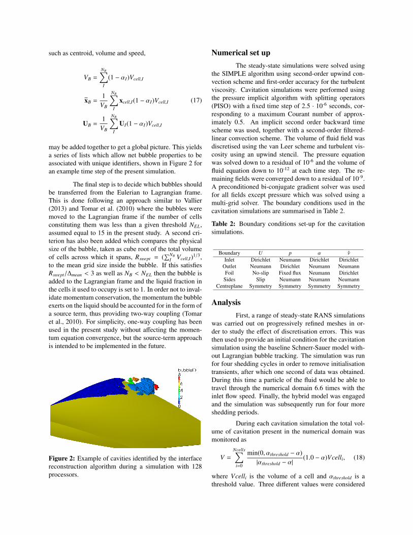
may be added together to get a global picture. This yieldsa series of lists which allow net bubble properties to beassociated with unique identifiers, shown in Figure 2 foran example time step of the present simulation.

The final step is to decide which bubbles shouldbe transferred from the Eulerian to Lagrangian frame.This is done following an approach similar to Vallier(2013) and Tomar et al. (2010) where the bubbles weremoved to the Lagrangian frame if the number of cellsconstituting them was less than a given threshold NEL,assumed equal to 15 in the present study. A second cri-terion has also been added which compares the physicalsize of the bubble, taken as cube root of the total volumeof cells across which it spans, Rswept = (

∑NBI Vcell,I)1/3,

to the mean grid size inside the bubble. If this satisfiesRswept/∆mean < 3 as well as NB < NEL then the bubble isadded to the Lagrangian frame and the liquid fraction inthe cells it used to occupy is set to 1. In order not to inval-idate momentum conservation, the momentum the bubbleexerts on the liquid should be accounted for in the form ofa source term, thus providing two-way coupling (Tomaret al., 2010). For simplicity, one-way coupling has beenused in the present study without affecting the momen-tum equation convergence, but the source-term approachis intended to be implemented in the future.

Figure 2: Example of cavities identified by the interfacereconstruction algorithm during a simulation with 128processors.

Numerical set upThe steady-state simulations were solved using

the SIMPLE algorithm using second-order upwind con-vection scheme and first-order accuracy for the turbulentviscosity. Cavitation simulations were performed usingthe pressure implicit algorithm with splitting operators(PISO) with a fixed time step of 2.5 · 10-6 seconds, cor-responding to a maximum Courant number of approx-imately 0.5. An implicit second order backward timescheme was used, together with a second-order filtered-linear convection scheme. The volume of fluid field wasdiscretised using the van Leer scheme and turbulent vis-cosity using an upwind stencil. The pressure equationwas solved down to a residual of 10-6 and the volume offluid equation down to 10-12 at each time step. The re-maining fields were converged down to a residual of 10-9.A preconditioned bi-conjugate gradient solver was usedfor all fields except pressure which was solved using amulti-grid solver. The boundary conditions used in thecavitation simulations are summarised in Table 2.

Table 2: Boundary conditions set-up for the cavitationsimulations.

Boundary U p α ν

Inlet Dirichlet Neumann Dirichlet DirichletOutlet Neumann Dirichlet Neumann NeumannFoil No-slip Fixed flux Neumann Dirichlet

Sides Slip Neumann Neumann NeumannCentreplane Symmetry Symmetry Symmetry Symmetry

AnalysisFirst, a range of steady-state RANS simulations

was carried out on progressively refined meshes in or-der to study the effect of discretisation errors. This wasthen used to provide an initial condition for the cavitationsimulation using the baseline Schnerr-Sauer model with-out Lagrangian bubble tracking. The simulation was runfor four shedding cycles in order to remove initialisationtransients, after which one second of data was obtained.During this time a particle of the fluid would be able totravel through the numerical domain 6.6 times with theinlet flow speed. Finally, the hybrid model was engagedand the simulation was subsequently run for four moreshedding periods.

During each cavitation simulation the total vol-ume of cavitation present in the numerical domain wasmonitored as

V =

Ncells∑i=0

min(0, αthreshold − α)|αthreshold − α|

(1.0 − α)Vcelli, (18)

where Vcelli is the volume of a cell and αthreshold is athreshold value. Three different values were considered

here: 0.1, 0.5, and 0.9, where 1.0 corresponds to waterwith no vapour content.

The pressure on the walls of the numerical cav-itation tunnel was monitored at six locations above thefoil. These were placed by performing a linear projec-tion of the pressure taps used in the experiment by Foeth(2008). Cartesian coordinates of the monitoring pointsare shown in Table 3.

Table 3: Locations of the probes placed to monitor pres-sures at the wall of the virtual cavitation tunnel. Origin atmid-chord, with x-axis pointing downstream and y-axisaligned with the span of the foil, as in Hoekstra et al.(2011).

Probe x [m] y [m] z [m]1 0.038 0.150 0.1502 0.001 0.150 0.1503 -0.013 0.150 0.1504 -0.028 0.150 0.1505 -0.043 0.150 0.1506 -0.066 0.150 0.150

RESULTS

Non-cavitating flow

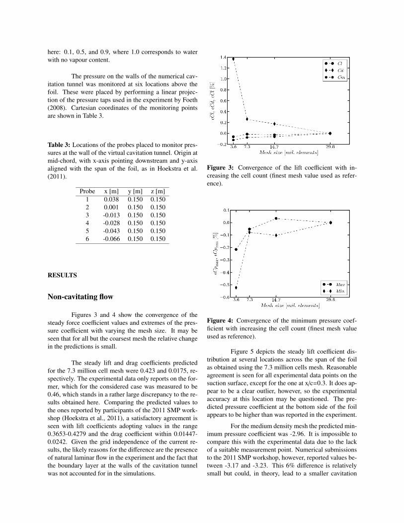
Figures 3 and 4 show the convergence of thesteady force coefficient values and extremes of the pres-sure coefficient with varying the mesh size. It may beseen that for all but the coarsest mesh the relative changein the predictions is small.

The steady lift and drag coefficients predictedfor the 7.3 million cell mesh were 0.423 and 0.0175, re-spectively. The experimental data only reports on the for-mer, which for the considered case was measured to be0.46, which stands in a rather large discrepancy to the re-sults obtained here. Comparing the predicted values tothe ones reported by participants of the 2011 SMP work-shop (Hoekstra et al., 2011), a satisfactory agreement isseen with lift coefficients adopting values in the range0.3653-0.4279 and the drag coefficient within 0.01447-0.0242. Given the grid independence of the current re-sults, the likely reasons for the difference are the presenceof natural laminar flow in the experiment and the fact thatthe boundary layer at the walls of the cavitation tunnelwas not accounted for in the simulations.

Figure 3: Convergence of the lift coefficient with in-creasing the cell count (finest mesh value used as refer-ence).

Figure 4: Convergence of the minimum pressure coef-ficient with increasing the cell count (finest mesh valueused as reference).

Figure 5 depicts the steady lift coefficient dis-tribution at several locations across the span of the foilas obtained using the 7.3 million cells mesh. Reasonableagreement is seen for all experimental data points on thesuction surface, except for the one at x/c=0.3. It does ap-pear to be a clear outlier, however, so the experimentalaccuracy at this location may be questioned. The pre-dicted pressure coefficient at the bottom side of the foilappears to be higher than was reported in the experiment.

For the medium density mesh the predicted min-imum pressure coefficient was -2.96. It is impossible tocompare this with the experimental data due to the lackof a suitable measurement point. Numerical submissionsto the 2011 SMP workshop, however, reported values be-tween -3.17 and -3.23. This 6% difference is relativelysmall but could, in theory, lead to a smaller cavitation

extent in the present simulation by not inducing quiteenough vaporisation near the leading edge of the foil.

Figure 5: Comparison of the steady-state, non-cavitatingpressure coefficient at various locations across the spanwith the experimentally reported values (Foeth, 2008).

Cavitation - flow fieldFor the baseline simulation of cavitating flow

without Lagrangian bubble tracking the mean lift coef-ficient was 0.412. This stands in satisfactory agreementwith values reported by Bensow (2011) who reported liftcoefficient values between 0.42 and 0.45 for simulationsusing RANS, DES and LES. The experimental results,however, report the mean lift coefficient to have been 0.53during the tests. The underestimation of lift suggests thatthe cavitation extent in the computations is too small.

Examining the mean pressure distribution at themid-span of the foil in Figure 6 reveals just that. One maysee how in the present results the characteristic plateaucorresponding to the presence of a cavity sheet drops off

around x/c=0.3, whereas in the experiment this was onlyreported to happen at x/c=0.4. In the measurement datathe pressure coefficient also appears to have increasedmuch more gradually in the region of cavity closure thanwhat was observed in the current simulation.

Similar observation regarding the mean extentof the attached cavities may be drawn by examining thedistribution of the average values of liquid volume frac-tion on the surface of the foil at mid-span, shown in Fig-ure 7. It may be seen that the attached cavity does notextend further downstream than x/c=0.3. It is interestingto note that the mean value first nears pure water aroundx/c=0.05, then moves back towards vapour and only latermoves to pure water region. This indicates that at somepoint during the cavitation cycle a gap exists between theattached cavity at the leading edge and one located furtherdownstream.

Figure 6: Mean pressure coefficient in cavitating condi-tion, also showing the standard deviation and experimen-tal data by Foeth (2008).

Figure 7: Mean volume fraction on the surface of thefoil, also showing the standard deviation.

Looking at a mean distribution of α along linesnormal to the foil surface at several x/c at mid span,depicted in Figure 8, shows that once the flow reachesx/c=0.35 cavitation seldom reaches the foil surface,which is consistent with the sampling on the surface ofthe foil. Notably though, at this station along the foilcavity structures may be seen to be much thicker thanthey are closer to the leading edge. As one moves fur-ther downstream the cavities appear to move away fromthe foil and the mean density quickly increases to nearlypure water at 0.6 x/c, which suggests that no cavitationstructures make it this far downstream.

A crucial quantity of interest is the frequencywith which the cavity sheet occurs and disappears in acycle. In order to deduce this it is useful to examinethe power spectral density functions of the unsteady lift

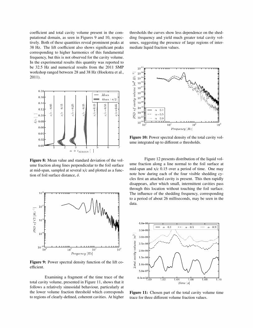
coefficient and total cavity volume present in the com-putational domain, as seen in Figures 9 and 10, respec-tively. Both of these quantities reveal prominent peaks at38 Hz. The lift coefficient also shows significant peakscorresponding to higher harmonics of this fundamentalfrequency, but this is not observed for the cavity volume.In the experimental results this quantity was reported tobe 32.5 Hz and numerical results from the 2011 SMPworkshop ranged between 28 and 38 Hz (Hoekstra et al.,2011).

Figure 8: Mean value and standard deviation of the vol-ume fraction along lines perpendicular to the foil surfaceat mid-span, sampled at several x/c and plotted as a func-tion of foil surface distance, δ.

Figure 9: Power spectral density function of the lift co-efficient.

Examining a fragment of the time trace of thetotal cavity volume, presented in Figure 11, shows that itfollows a relatively sinusoidal behaviour, particularly atthe lower volume fraction threshold which correspondsto regions of clearly-defined, coherent cavities. At higher

thresholds the curves show less dependence on the shed-ding frequency and yield much greater total cavity vol-umes, suggesting the presence of large regions of inter-mediate liquid fraction values.

Figure 10: Power spectral density of the total cavity vol-ume integrated up to different α thresholds.

Figure 12 presents distribution of the liquid vol-ume fraction along a line normal to the foil surface atmid-span and x/c 0.15 over a period of time. One maynote how during each of the four visible shedding cy-cles first an attached cavity is present. This then rapidlydisappears, after which small, intermittent cavities passthrough this location without touching the foil surface.The influence of the shedding frequency, correspondingto a period of about 26 milliseconds, may be seen in thedata.

Figure 11: Chosen part of the total cavity volume timetrace for three different volume fraction values.

Figure 12: Temporal evolution of the volume fraction atmid-span and x/c=0.15 plotted as a function of foil sur-face distance, δ.

Figure 16 presents a series of consecutive in-stantaneous pictures showing cavitation extent in theoriginal study by Foeth (2008) and the corresponding iso-contours from the present simulation. One may note howa large, developed cavity sheet grows to its maximumsize, then rapidly necks close to the leading edge dueto the passage of a re-entrant jet, which is followed bythe characteristic v-shaped notch in the sheet as it is fill-ing with vapour again. One may see that the overall be-haviour of the flow is similar to the one observed in theexperiment. A major difference is that the stream-wiseextent of the sheet is less in the present simulation, as al-ready made evident from the surface pressure data. Like-wise, cavitation does not extend as far span-wise. Be-cause of this, the sheet is far more stable off-centrelinethan in the experiment, which leads to the re-entrant jetnot occurring along the entire width of the sheet the wayit was measured, but instead this behaviour may only beseen at the central part of the foil.

Cavitation - tunnel wall pressuresFigure 13 presents cavitation-induced pressure

at the top wall of the virtual cavitation tunnel directlyabove the leading edge of the foil. The signal shows fluc-tuations of approximately ±3% of the reference pressureand, at the first glance, does not show direct dependenceon the shedding frequency. However, spectral analysis,shown in Figure 14, indicates that the wall pressure is di-rectly related to the cavity sheet behaviour and its higherharmonics.

Furthermore, data for other receivers placedalong the centreline of the foil visible in Figure 14 showsthat all of the investigated locations experience very sim-ilar pressure fluctuations. A closer analysis of how thepeak value of the first harmonic varies with distance

from the leading edge of the foil is depicted in Figure15. The magnitude of wall pressure fluctuations maybe seen to decay with the distance from the location ofthe most prominent cavitation behaviour. Intuitively, onemight expect this reduction in amplitude to follow an in-verse square law, given that cavitation tends to act as amonopole noise source (Park et al., 2009b, Seol et al.,2005). Comparing the data to a least-squares quadraticfit indicates, however, that in the present data receiverscloser to the leading edge do not see as much reductionin the fluctuations as could be expected.

Figure 13: Wall pressure as a function of outlet pressurepredicted for a probe above the leading edge of the foil atthe centreline (probe 6).

Figure 14: Power spectral density function of the wallpressure for a series of probes placed along the centrelineof the foil, from the trailing edge (probe 1) to the leadingedge (probe 6).

Figure 15: Decay of peak wall pressure PSD around thefirst harmonic (38 Hz) with distance from the foil leadingedge, also showing a quadratic least-squares fit.

Lagrangian bubble trackingFigure 17 shows the distribution of Lagrangian

bubbles at an instant in the cavitation cycle similar to theone in Figure 16 g). One may note that the volume-of-fluid field behaves in a very similar when the hybridmodel is used, yielding similar iso-contours. An impor-tant observation is also that while the baseline mass trans-fer model fails to convect cavities down to the trailingedge to the foil, which was observed in the experiment,the hybrid model does this successfully.

Closer analysis of where the Lagrangian bubblesget created shows that there are two primary scenariosin which transfer from the Eulerian frame occurs. First,when a well-defined cavity with high vapour fraction sig-nificantly reduces in size. The second instance, by far ap-pearing to be more common in the present simulation, iswhen there exists a region of intermediate vapour fractionvalues and when at some point, either by becoming physi-cally separated or when local volume fractions exceed thethresholds, a certain sub-region gets identified as a sepa-rate cavity by the reconstruction algorithm. In Figure 17this may be seen to occur primarily close to the centre-line of the foil where large interface displacements andvelocities take place, causing injection of relatively largeLagrangian bubbles, predominantly just after the occur-rence of the re-entrant jet. This appears to stand in goodagreement with the experimental observations. A secondregion where Lagrangian bubbles get created is at around35% of span where the cavity sheet also experiences sub-stantial deformations. This behaviour may also be seenin the experimental data (Figure 16 a) and c)), althoughmore bubbles appear to have been created at this loca-tion during experimental tests. This discrepancy could bedue to the unsteadiness of the volume fraction field beingunder-predicted and not necessarily shortcomings of theEuler-to-Lagrange transition algorithm.

a) Experiment b) CFD

c) Experiment d) CFD

e) Experiment f) CFD

g) Experiment h) CFD

i) Experiment j) CFD

Figure 16: Flow snapshots of experimental data by Foeth(2008) and the iso-contours of the volume fraction field(α = 0.5). CFD data only shows half of the foil, in accor-dance with how the calculation was set up.

a) Zoom-in on the leading edge

b) Top view (as in Figure 16 g) and h))

c) Isometric view showing the wake

Figure 17: View of an instantaneous distribution of La-grangian bubbles (red spheres) and the fluid volume frac-tion (blue, α = 0.5) at a point in the cavitation cycle sim-ilar to the one shown in Figures 16 g) and h).

A key aim of the present study was to investi-gate how much the Lagrangian bubbles contribute to theinduced wall pressures, which is depicted in Figures 18and 19 in the form of time- and frequency-domain plots.The former shows pressure at the probe above the leadingedge of the foil over the duration of approximately onecavitation cycle. One may note that the pressure causedby the presence of small bubbles exhibits a broadband na-ture without immediately obvious concentrations alongthe time axis. One would expect that the spikes in theEulerian pressure field, visible around times 0.006 and0.012 s, to cause an increased likelihood of collapse ofthe Lagrangian bubbles, thus further reinforcing the pre-dicted noise.

Turning to Figure 19 shows that including thepressure induced by the Lagrangian bubbles in the spec-tral analysis causes an 8 dB increase in the first harmonic

and makes the higher harmonics more clearly definedthan when just the Eulerian pressure is considered. Onemay thus more readily see the relationship between therise in local pressure causing an increased number of La-grangian collapses and thus contributing more to the pre-dicted wall pressures than in the time series in Figure18. It should be noted that the low-frequency range ofthe spectra in Figure 19 is different than in Figure 14 isdue to the hybrid model simulation having been run for asmaller number of cavitation cycles due to the increasedcomputational cost.

In total, over 15000 Lagrangian bubbles havebeen introduced to the numerical domain over the periodof 4 cavitation cycles. It has thus proven challenging toanalyse their individual lifetimes in detail. An interest-ing hand-picked example is shown in Figure 20 wherethe time history of the evolution of the radius of a bub-ble and the external pressure acting on it are shown. Onemay note how first the bubble was in a region of constantpressure and thus experienced little variation in radius tothe equilibrium assumption. It then experienced a rise inexternal pressure, leading to a decrease in radius. It wasthen swept closer to the centreline of the foil to a regionof lower pressure, leading to a significant expansion, fol-lowed by a collapse and a series of rebounds. A suddenspike in the external pressure may then be seen whichappears to have altered the oscillation frequency and re-duced the amplitude of the radius. The bubble then wasconvected by the flow towards the outlet, which was ac-companied by a steady rise in local pressure and decay ofthe oscillation of the radius.

Figure 18: Direct Eulerian wall pressure at probe 6 alsoshowing values with superimposed Lagrangian bubblespressures.

Figure 19: Power spectral density function of the directCFD and combined Euler-Lagrange wall pressures at thelocation of probe 6.

Figure 20: Time history of the radius and external pres-sure acting on a selected bubble which was created 0.1 soff-centreline close to the beginning of the simulation.

DISCUSSION

It has been shown, based on the distribution of pressurecoefficient as well as the mean and instantaneous localvalues of the volume fractions, that the predicted cavi-tation extents are smaller than what was reported in theexperimental data. The predicted shedding frequency of38 Hz is also higher than 32.5 Hz originally measured byFoeth (2008). It is likely that both of these discrepan-cies are due to the same underlying issue, since a morepronounced cavity sheet could be expected to take moretime to grow to its full extent, which would then lowerthe frequency of the complete cycle. It has been seen thatthe predicted steady-state solution is grid-independent,both in terms of forces and local pressure coefficient, al-though discrepancies have been observed in the lift being

too low compared to the experimental data and the min-imum pressure coefficient being higher than in other nu-merical studies. This could potentially explain the under-prediction of cavitation extent. On the other hand, thestudy by Bensow (2011) also reported under-predictionof the cavity extents while quoted shedding frequenciescloser to the experimentally measured value. Anotherpossible reason for the current discrepancies could be thesimplification made when assuming a constant nuclei sizeand density, which would not have been true in reality, orslight misalignment of the foil in the tunnel during thetests. Further sensitivity studies are therefore needed totruly explore the origin of this behaviour. Nonetheless,enough agreement may be seen between the present andpublicly available data to support subsequent discussion.

As expected, the wall pressures induced by thecavitation were predicted to be primarily dependent onthe shedding frequency. The data did also show, however,a substantial amount of higher harmonics, most likely as-sociated with more local phenomena, such as formationof smaller clouds and local velocities of the cavity inter-face. This hints at the importance of three-dimensionaleffects in examining cavitation induced pressures. On thisnote, it has also been seen that while from a far-field per-spective the cavitation-related noise source may be com-pact, in the near-field this is not necessarily the case.

Comparison of the predicted and experimentallyobserved distribution and location of Lagrangian bubblesduring the cavitation cycle has revealed promising agree-ment. This indicates that, despite the simplicity of itscurrent implementation, the hybrid Eulerian-Lagrangiancavitation model accounts for the dominant physical phe-nomena. A key observation in this regard has been theimportance of local cavity interface deformations, mostlikely related to the presence of shear layers, on where re-gions of intermediate volume fractions occur and spawnpotential injection sites for Lagrangian bubbles. Al-though no experimental data exist in the public domain tovalidate the predicted wall pressures, the observed broad-band contributions of the small-scale bubbles superim-posed on the underlying low-frequency oscillations in-duced by the large-scale cavity sheet and clouds standin qualitative agreement with what is understood aboutmulti-scale cavitation noise (Brennen, 2009a, Bretschnei-der et al., 2008, Matusiak, 1992).

Several areas for improvement have been iden-tified in the current multi-scale cavitation model. It hasbeen seen that certain Lagrangian bubbles grow in sizegreater than the local grid size, which would justify trans-ferring them back to the Eulerian frame of reference(Hsiao et al., 2014). Likewise, a small number of theLagrangian bubbles were seen to come in contact withthe cavities defined by the volume of fluid. In reality,

one would expect the smaller bubbles to merge with theirlarger counterpart or at least interact with the cavity inter-face, which is not accounted for at the moment. The samegoes for the interaction of Lagrangian bubbles betweenthemselves (Vallier, 2013). The latter is, however, ex-pected to be computationally expensive due to the addedcost of a global reduce operation required for bubbles ineach sub-domain to contain information on all the otherLagrangian parcels in the simulation. Finally, it has beenseen that a vast amount of data gets generated from theLagrangian tracking algorithm which makes it difficult toutilise using more basic CFD post-processing techniques.It is thus hoped that more robust and statistically soundapproaches can be devised in the future to better informthe user on what the results mean in practice.

CONCLUSIONS

The present multi-scale cavitation model predicts cavita-tion behaviour which stands in qualitative agreement withthe experimental observations. The broadband noise in-duced by the Lagrangian cavities was not predicted to af-fect the dominant, low-frequency harmonics of the wallpressures significantly, but was observed to extend therange of frequencies generated by cavitation well abovea kilohertz. It is believed that, following the inclusionof several additional physical mechanisms, the currentmodel will form a useful tool for cross-examination ofcavitation tunnel noise measurements and will contributetowards a better understanding of ship noise.

ACKNOWLEDGEMENTS

The authors would like to acknowledge the use of theIridis 4 supercomputer of University of Southampton,UK, on which the discussed simulations have been con-ducted.

REFERENCES

Aktas, B., Turkmen, S., Sampson, R., Shi, W., Fitzsim-mons, P., Korkut, E., and Atlar, M., “Underwater ra-diated noise investigations of cavitating propellers usingmedium size cavitation tunnel tests and full-scale trials,”Fourth International Symposium on Marine Propulsors(SMP), Austin, Texas, USA, June, 2015.

Bensow, R., “Simulation of the unsteady cavitation on thethe Delft Twist11 foil using RANS, DES and LES,” 2ndInternational Symposium on Marine Propulsors, Ham-burg, Germany, June, 2011.

Bertschneider, H., Bosschers, J., Choi, G. H., Ciappi,E., Farabee, T., Kawakita, C., and Tang, D., “SpecialistCommittee on Hydrodynamic Noise,” Technical report,ITTC, 2014.

Brennen, C. E., “Cavitation,” Fundamentals of Multi-phase Flow, chapter 5, pages 97–115. Cambridge Uni-versity Press, Cambridge, 2 edition, 2009a ISBN 978-0-521-13998-4.

Brennen, C. E., “Bubble growth and collapse,” Fun-damentals of Multiphase Flow, chapter 4, pages 73–96. Cambridge University Press, Cambridge, 2 edition,2009b ISBN 978-0-521-13998-4.

Bretschneider, H., Lydorf, U., and Johannsen, C., “Ex-perimental Investigation to Improve Numerical Modelingof Cavitation,” Technical report, HSVA GmbH, 2008.

Brooker, A. and Humphrey, V. F., “Measurement of Ra-diated Underwater Noise from a Small Research Vesselin Shallow Water,” A. Yucel Odabas Colloquium Series,pages 47–55, 6th-7th November, Istanbul, Turkey, 2014.

Chahine, G., “Nuclei effects on cavitation inception andnoise,” 5th Symposium on Naval Hydrodynamics, pages8–13, St. John’s, Newfoundland and Labrador, Canada,August, 2004.

EU FP7, “AQUO Project,”, 2014a URL http://www.aquo.eu/.

EU FP7, “SONIC Project,”, 2014b URL http://www.sonic-project.eu/.

Foeth, E. J., Doorne, C. W. H., van Terwisga, T., andWieneke, B., “Time resolved PIV and flow visualiza-tion of 3D sheet cavitation,” Experiments in Fluids,40(4):503–513, 2006 ISSN 0723-4864 doi: 10.1007/

s00348-005-0082-9.

Foeth, E., “The structure of three-dimensional sheet cav-itation,” PhD thesis, TU Delft, 2008.

Hildebrand, J., “Anthropogenic and natural sources ofambient noise in the ocean,” Marine Ecology ProgressSeries, 395:5–20, dec 2009 ISSN 0171-8630 doi:10.3354/meps08353.

Hoekstra, M., van Terwisga, T., and Foeth, E. J., “SMP11Workshop - Case 1: DelftFoil,” Second InternationalSymposium on Marine Propulsors, Hamburg, Germany,2011.

Hsiao, C., Ma, J., Chahine, G. L., Ynaflow, D., and Nc,I., “Multi-Scale Two-Phase Flow Modeling of Sheet andCloud Cavitation,” 30th Symposium on Naval Hydro-dynamics, Hobart, Tasmania, Australia, 2-7 November,2014.

Hsiao, C. T. and Chahine, G. L., “Scaling of tip vortexcavitation inception for a marine open propeller,” 27thSymposium on Naval Hydrodynamics, Seoul, Korea, Oc-tober, 2008.

Ianniello, S., Muscari, R., and Mascio, A., “Ship un-derwater noise assessment by the acoustic analogy. PartI: nonlinear analysis of a marine propeller in a uni-form flow,” Journal of Marine Science and Technol-ogy, 18(4):547–570, jul 2013 ISSN 0948-4280 doi:10.1007/s00773-013-0227-0.

Ianniello, S. and Bernardis, E. D., “Farassat s formula-tions in marine propeller hydroacoustics,” InternationalJournal of Aeroacoustics, 14(1 & 2):87–103, 2015.

Koop, A. H., “Numerical simulation of unsteady three-dimensional sheet cavitation,” PhD thesis, University ofTwente, Enschede, The Netherlands, 2008.

Lidtke, A. K., Turnock, S. R., and Humphrey, V. F.,“Characterisation of sheet cavity noise of a hydrofoil us-ing the Ffowcs Williams-Hawkings acoustic analogy,”Computers & Fluids, 130:8–23, 2016 doi: 10.1016/j.compfluid.2016.02.014.

Lloyd, T. P., Lidtke, A. K., Rijpkema, D., Van Wijn-gaarden, E., Turnock, S. R., and Humphrey, V. F., “Us-ing the FW-H equation for hydroacoustics of propellers,”Numerical Towing Tank Symposium (NuTTS), Cortona,Italy, 2015.

Matusiak, J., “Pressure and noise induced by a cavitatingmarine screw propeller,” PhD thesis, Helsinki Universityof Technology, 1992.

Menter, F. R., Kuntz, M., and Langtry, R., “Ten Years ofIndustrial Experience with the SST Turbulence Model,”Hanjalic, K., Nagano, Y., and Tummers, M., editors, Tur-bulence, Heat and Mass Transfer 4, pages 625 – 632, An-talya, Turkey, 12-17 October, 2003. Begell House, Inc.

Nordin, N. P. A., “Complex chemistry modelling ofdiesel spray combustion,” PhD thesis, Chalmers Univer-sity of Technology, 2001.

Park, C., Seol, H., Kim, K., and Seong, W., “A study onpropeller noise source localization in a cavitation tunnel,”Ocean Engineering, 36(9-10):754–762, jul 2009a ISSN00298018 doi: 10.1016/j.oceaneng.2009.04.005.

Park, K., Seol, H., Choi, W., and Lee, S., “Numerical pre-diction of tip vortex cavitation behavior and noise con-sidering nuclei size and distribution,” Applied Acous-tics, 70(5):674–680, may 2009b ISSN 0003682X doi:10.1016/j.apacoust.2008.08.003.

Plesset, M. S. and Prosperetti, A., “Bubble dynamics andcavitation,” Annual Review of Fluid Mechanics, 9(1):145–185, 1977.

Sauer, J. and Schnerr, G. H., “Development of a newcavitation model based on bubble dynamics,” Zeitschrift

fur Angewandte Mathematik und Mechanik, 81:561–562,2001.

Seo, J. H., Moon, Y. J., and Shin, B. R., “Predictionof cavitating flow noise by direct numerical simulation,”Journal of Computational Physics, 227(13):6511–6531,jun 2008 ISSN 00219991 doi: 10.1016/j.jcp.2008.03.016.

Seol, H., “Time domain method for the prediction ofpressure fluctuation induced by propeller sheet cavita-tion: Numerical simulations and experimental valida-tion,” Ocean Engineering, 72:287–296, nov 2013 ISSN00298018 doi: 10.1016/j.oceaneng.2013.06.030.

Seol, H., Suh, J.-C., and Lee, S., “Development of hybridmethod for the prediction of underwater propeller noise,”Journal of Sound and Vibration, 288(1-2):345–360, nov2005 ISSN 0022460X doi: 10.1016/j.jsv.2005.01.015.

Spalart, P. R. and Allmaras, S. R., “A one equation tur-bulence model for aerodinamic flows,” AIAA Journal, 94(439), 1992.

Sunil, M., Keith, T. G., and Nikolaidis, E., “Numericalsimulation of traveling bubble cavitation,” InternationalJournal of Numerical Methods for Heat & Fluid Flow, 16(4):393–416, 2006.

Tomar, G., Fuster, D., Zaleski, S., and Popinet, S., “Mul-tiscale simulations of primary atomization,” Computersand Fluids, 39(10):1864–1874, 2010 ISSN 00457930doi: 10.1016/j.compfluid.2010.06.018.

Tomita, Y. and Shima, A., “On the behavior of a sphericalbubble and the impulse pressure in a viscous compress-ible liquid,” Bulletin of the JSME, 20(149):1453–1460,1977.

Urik, R. J., “Ambient noise in the sea,” Technical report,1984.

Vallier, A., “Simulations of cavitation-from the largevapour structures to the small bubble dynamics,” PhDthesis, Lund University, 2013.

Wu, X. C., Wang, Y. W., and Huang, C. G., “Effect ofmesh resolution on large eddy simulation of cloud cavi-tating flow around a three dimensional twisted hydrofoil,”European Journal of Mechanics B / Fluids, 55:229–240,2016 doi: 10.1016/j.euromechflu.2015.09.011.

Yakubov, S., Cankurt, B., Abdel-Maksoud, M., andRung, T., “Hybrid MPI/OpenMP parallelization of anEuler-Lagrange approach to cavitation modelling,” Com-puters and Fluids, 80(1):365–371, 2013 ISSN 00457930doi: 10.1016/j.compfluid.2012.01.020.

DISCUSSION

Rickard Bensow, Professor, Chalmers University ofTechnology, Gothenburg, Sweden

The authors present a well written and inter-esting paper on the application of a hybrid Eulerian-Lagrangian cavitation modelling approach for pressurepulse simulations. The idea of how to develop the mod-elling itself is not new, but the paper presents a compre-hensive description of the authors interpretation and im-plementation and a nice application.

1. The addition of the Lagrangian bubbles is moti-vated by the intrinsic inability of an incompressibleEulerian approach to account for cavity collapsebehaviour and thus its broad band contribution. Iagree on this, but perhaps one could have com-mented that there are other contributions to broadband noise/pressure pulses (in sheet or tip cavitydynamics) that the Eulerian method has better po-tential to capture; an argument actually strengthen-ing the hybridisation.

2. As I interpret the methodology, its a one-way cou-pling such that the Eulerian simulation determinesthe flow pressure field, while the integration of thepressure from Lagrangian bubble dynamics is onlyused to sample at the probe location. Is this cor-rect? If so, could the authors comment on howa two way coupling could be realised and how itwould affect the flow results?

3. Regarding the discrepancy in lift coefficient, therehas been numerical results published which givebetter agreement with experiments than was re-ported at the 2011 SMP workshop. As the meshstudy indicated well converged results, my guesswould be that this is then a result of the turbulencemodel chosen. It would thus be interesting to seean additional run with an alternative model.

4. It would be interesting to see the sheet cavity out-line in relation to the mesh resolution on the suc-tion side of the foil. I suspect that the mesh reso-lution, although fine at 7.3 M cells for half foil andcertainly good enough for wetted flow, is too lowaround the sheet and that this, then, is one reasonfor the under predicted cavity extent.As nicely pointed out be the authors, the trans-ported shed vapour seem to be captured by the La-grangian bubbles, but the sheet dynamics may behampered by the seemingly low resolution a bit ofthe foil surface.

I enjoyed reading the paper with its well presented con-tent and Im much looking forward to further discussionat the symposium.

AUTHORS’ REPLY

We would like to thank the discusser for the in-sightful comments which increased the value of the paper.Specific questions and remarks are addressed below.

Question 1: The discusser raises a very impor-tant point and the original discussion in the paper over-simplified the problem to a degree. It has been shown inthe literature that collapsing cavity sheets and tip cavita-tion may contribute to the broadband noise spectrum buta pure Lagrangian approach would likely be insufficientto resolve these accurately.

Question 2: The summary of the method pro-vided by the discusser is correct - the initial model pre-sented in the paper assumed the Lagrangian bubbles to beconvected by the fluid with the assumption that their vol-ume fraction is relatively low. This was later found not tobe true at all times, as may be seen, for instance, in Fig-ure 17. It shows that often the bubbles cluster together inrelative proximity and sometimes grow in size consider-ably, as seen in Figure 20. This implies that interactionsbetween bubbles and the action of the Lagrangian bub-bles on the flow should be considered in order to achievemore accurate modelling.Including a source term in the momentum equation couldrelatively easily be added to reflect the change in mo-mentum of the fluid caused by it carrying a mass of La-grangian bubbles. Furthermore, one could also imple-ment an algorithm searching the neighbourhood of eachparticle for other bubbles. In case a collision was de-tected, semi-empirical criteria could be used in order todetermine whether the bubbles will coalesce or bounce,and how this interaction will occur. A detailed discussionof the topic is given, for instance, by Vallier (2013).

Question 3: The reviewer is right to pointout that there have been several more recent studies re-porting better agreement with the experimental values.For instance, Wu et al. Wu et al. (2016) used wall-modelled LES on a 10 million cells grid and achievedvery good agreement with the experimental values inthe non-cavitating condition (authors did not report onthe forces predicted for cavitation conditions). Sincein the present simulations the solution is deemed grid-independent future work will have to focus on identify-ing the exact reason for the observed discrepancies, mostlikely associated with the turbulence model.Following the presented simulations two additional runswere carried out on the 7.3 M grid using LES with theSmagorinsky model and an implicit model (ILES). The

present mesh was too coarse for LES to resolve the near-wall region, with resolution lacking in the x- and z-directions, and thus a wall model was used. Both ofthe simulations predicted similar lift coefficient values aswell as very comparable flow features. The studies werepreliminary in nature and so the answers they providedmust be treated with caution, but they do point to the Eu-lerian cavitation model and its settings being responsiblefor the observed discrepancies.

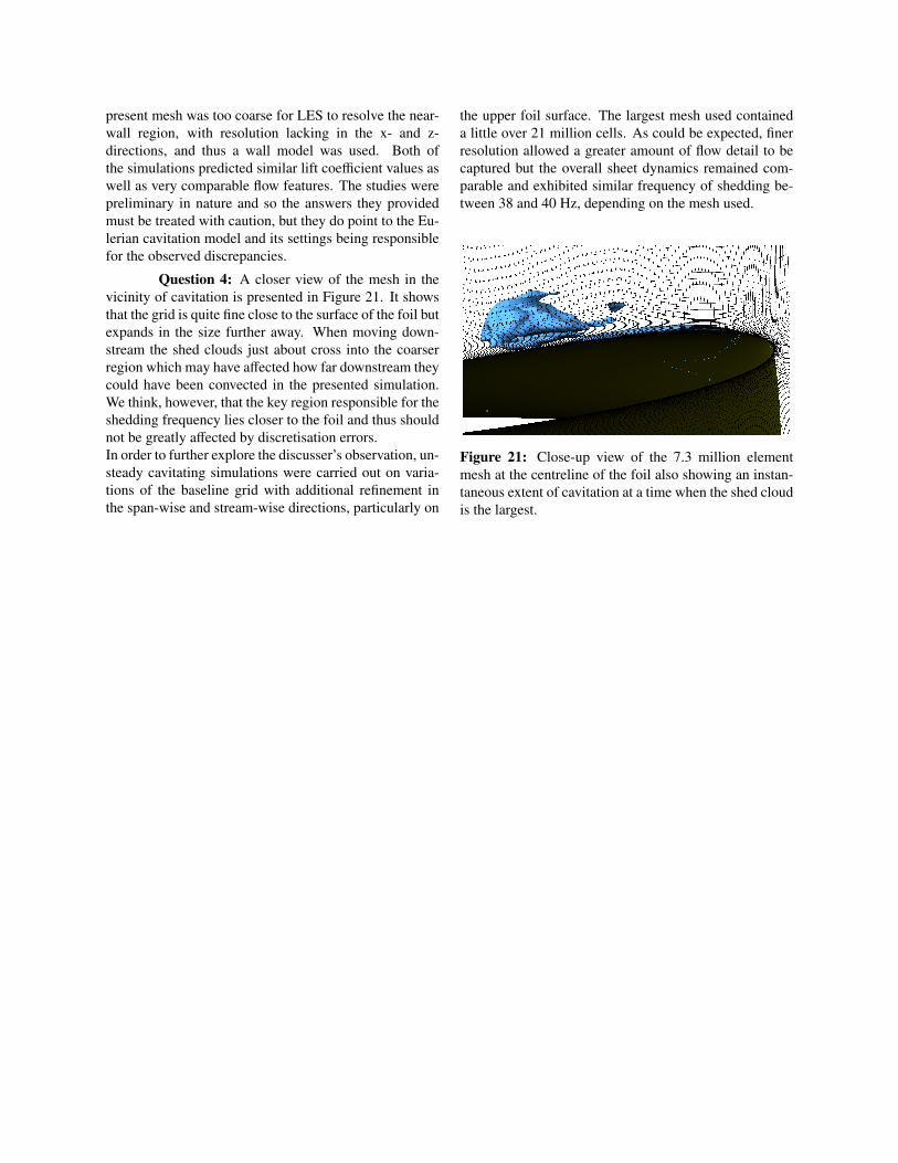
Question 4: A closer view of the mesh in thevicinity of cavitation is presented in Figure 21. It showsthat the grid is quite fine close to the surface of the foil butexpands in the size further away. When moving down-stream the shed clouds just about cross into the coarserregion which may have affected how far downstream theycould have been convected in the presented simulation.We think, however, that the key region responsible for theshedding frequency lies closer to the foil and thus shouldnot be greatly affected by discretisation errors.In order to further explore the discusser’s observation, un-steady cavitating simulations were carried out on varia-tions of the baseline grid with additional refinement inthe span-wise and stream-wise directions, particularly on

the upper foil surface. The largest mesh used containeda little over 21 million cells. As could be expected, finerresolution allowed a greater amount of flow detail to becaptured but the overall sheet dynamics remained com-parable and exhibited similar frequency of shedding be-tween 38 and 40 Hz, depending on the mesh used.

Figure 21: Close-up view of the 7.3 million elementmesh at the centreline of the foil also showing an instan-taneous extent of cavitation at a time when the shed cloudis the largest.