Multi-layer evolution schemes for the finite-dimensional quantumsystems in external fields.

Ochbadrakh Chuluunbaatar,Alexander Gusev,Vladimir Gerdt,Michail Kaschiev,Vitaly Rostovtsev,Yoshio Uwano,Sergue Vinitsky

This talk is prepared to the 4th International Workshop ”Quantum Physics andCommunication”, QPC 2007, Dubna, Russia, 15 - 19 October, 2007.

1. General formulation and operator-difference multi-layer calculation scheme

Let us consider the Cauchy problem for the time-dependent operator equation on thetime interval t ∈ [t0, T ]

ı∂Ψ(t)

∂t= H(t)Ψ(t), Ψ(t0) = Ψ0, (1)

where H(t) is a linear self-adjoint operator. We rewrite Eq. (1) in terms of an unitaryevolution operator U(t, t0, λ) with a complementary formal parameter λ carrying theinitial state Ψ0 to the solution Ψ(t) in the form

ı∂U(t, t0, λ)

∂t= λH(t)U(t, t0, λ), U(t, t, λ) = 1, (2)

which considered in the uniform grid

Ωτ [t0, T ] = t0, tk+1 = tk + τ, tK = T (3)

with time step τ , in the time interval [t0, T ]. The complementary formal parameter λwill be replaced to be λ = 1 later. We express the unitary operator U(tk+1, tk , λ)carrying the solution Ψ(tk) at t = tk to the one Ψ(tk+1) at t = tk+1 in the form 1 2

Ψ(tk+1) = U(tk+1, tk , λ)Ψ(tk), (4)

U(tk+1, tk , λ) = exp“

−ıτA(M)k (tk+1, λ)

”

+ O(τ2M+1).

1Puzynin I V, Selin A V and Vinitsky S I 1999 Comput. Phys. Commun. 123 1–62Puzynin I V, Selin A V and Vinitsky S I 2000 Comput. Phys. Commun. 126 158–161

We start with the power-series expansion of A(M)k (t) ≡ A

(M)k (t, λ) in terms of the

formal parameter λ,

A(M)k (t, λ) =

ı

τ

2MX

j=1

λjA(j)k(t), A(M)k (tk , λ) = 0, (5)

where the coefficients A(j)(t) ≡ A(j)k(t) are evaluated from the operator-identity 3

− ıλH(t) =

n+Σqi=1

li≤2MX

n=1;q=0;l1,...,lq=1

λn+Σqi=1li

(q + 1)!(adA(l1)(t)) . . . (adA(lq)(t))

.

A(n) (t). (6)

Here the linear operator (adA) : L(X) → L(X) (L(X) is the space of linear operators)is defined for operators A,B ∈ L(X) in the form (adA)B = [A,B] ≡ AB −BA andhave the following properties: (adA)0B = B, (adA)jB = (adA)j−1(adA)B. Notethat the dot over the operator A(n)(t) means the partial derivation,.

A(n) (t) = ∂tA(n)(t), in t. Equating the coefficients at the same powers of λ in bothsides of (6), we obtain a set of the first-order differential equations.

3Wilcox R M 1967 J. Math. Phys. 8 962–982

For example, the first three equations reads as

.

A(1) (t) = −ıH(t),

.

A(2) (t) = −(adA(1)(t))

.

A(1) (t)

2, (7)

.

A(3) (t) = −(adA(2)(t))

.

A(1) (t)

2−

(adA(1)(t))2

.

A(1) (t)

6−

(adA(1)(t)).

A(2) (t)

2,

we obtain

A(1)(t) = −ıΥ11(t), A(2)(t) =

1

2Υ2

21(t), A(3)(t) =ı

6

`

Υ3123(t) + Υ3

321(t)´

. (8)

The fourth-order term is similarly calculated. We find

A(4)(t) =1

12

`

Υ41432(t) + Υ4

1234(t) + Υ44312(t) + Υ4

2341(t)´

. (9)

Here

Υnl1,...,ln

(t) =

Z t

tk

dt1

Z t1

tk

dt2 . . .

Z tn−1

tk

dtn(adH(tl1 )) . . . (adH(tln−1))H(tln ). (10)

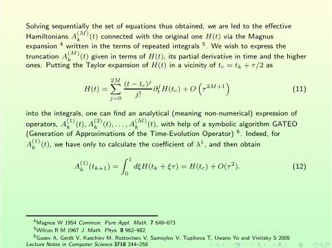
Solving sequentially the set of equations thus obtained, we are led to the effective

Hamiltonians A(M)k (t) connected with the original one H(t) via the Magnus

expansion 4 written in the terms of repeated integrals 5. We wish to express the

truncation A(M)k (t) given in terms of H(t), its partial derivative in time and the higher

ones. Putting the Taylor expansion of H(t) in a vicinity of tc = tk + τ/2 as

H(t) =2MX

j=0

(t − tc)j

j!∂j

tH(tc) +O“

τ2M+1”

(11)

into the integrals, one can find an analytical (meaning non-numerical) expression of

operators, A(1)k (t), A

(2)k (t), . . . , A

(M)k (t), with help of a symbolic algorithm GATEO

(Generation of Approximations of the Time-Evolution Operator) 6. Indeed, for

A(1)k (t), we have only to calculate the coefficient of λ1, and then obtain

A(1)k (tk+1) =

Z 1

0dξH(tk + ξτ) = H(tc) + O(τ2). (12)

4Magnus W 1954 Commun. Pure Appl. Math. 7 649–6735Wilcox R M 1967 J. Math. Phys. 8 962–9826Gusev A, Gerdt V, Kaschiev M, Rostovtsev V, Samoylov V, Tupikova T, Uwano Yo and Vinitsky S 2005

Lecture Notes in Computer Science 3718 244–258

To show the complexity of calculations, we present the first three approximations of

the exponential (4) for the final effective Hamiltonians A(M)k ≡ A

(M)k (tk+1) in the

form A(M)k = A

(M)k + ıA

(M)k

A(1)k = H,

A(1)k = 0,

A(2)k = A

(1)k +

τ2

24

..

H, (13)

A(2)k = A

(1)k +

τ2

12(adH)

.

H,

A(3)k = A

(2)k +

τ4

1920

....

H − τ4

720(adH)2

..

H − τ4

240(ad

.

H)2H,

A(3)k = A

(2)k − τ4

480(ad

...

H )H +τ4

480(ad

..

H).

H +τ4

720(adH)3

.

H,

where H ≡ H(tc),.

H≡ ∂tH(t)|t=tc, . . .

1.1. Generalized [M/M ] Pade approximation

Application to the exponential operator of the generalized [M/M ] Pade approximationyields

exp“

−ıτA(M)k

”

=1Y

ζ=M

Tζk + O(τ2M+1), (14)

Tζk =

0

@I +τα

(M)ζ A

(M)k

2M

1

A

−10

@I +τα

(M)ζ A

(M)k

2M

1

A ,

where I is the unit operator and the overline indicates the complex conjugate

operation. The coefficients, α(M)ζ (ζ = 1, . . . ,M , M ≥ 1), stand for the roots of the

polynomial equation, 1F1(−M,−2M, 2Mı/α) = 0, where 1F1 is the confluenthypergeometric function.

Table: The real and imaginary parts of the coefficients α(M)ζ

, M = 1, 2, 3, ζ = 1, . . . , M

M ζ ℜα(M)ζ ℑα(M)

ζ

1 1 +0.0 −1.02 1 −0.57735026918962576450914878050 −1.02 2 +0.57735026918962576450914878050 −1.03 1 −0.81479955424892281841473623156 −0.854056730651663465265799408863 2 +0.0 −1.291886538696673069468401182283 3 +0.81479955424892281841473623156 −0.85405673065166346526579940886

Table 1 lists the values of the coefficients, α(M)ζ for M = 1, 2, 3, in GATEO. The

coefficients α(M)ζ have the following properties: ℑα(M)

ζ < 0 and 0.6 < |α(M)ζ | < µ−1,

where µ ≈ 0.28 is the root of equation µ exp(µ+ 1) = 1 7. Note that the condition

τ < 2Mµ||A(M)k (t)||−1 guarantees the validity of the approximation (14) for any

bounded operator A(M)k (t).

7Puzynin I V, Selin A V and Vinitsky S I 1999 Comput. Phys. Commun. 123 1–6

1.2. The operator-difference scheme of the evolution operator

We are now in a position to obtain the transition from Ψ(tk) to Ψ(tk+1), by using theapproximation (14) of the evolution operator in (4). To make it, we rewrite thetransition in terms of the auxiliary functions defined by

ψ0k = Ψ(tk),0

@I +τα

(M)ζ A

(M)k

2M

1

Aψζ/Mk =

0

@I +τα

(M)ζ A

(M)k

2M

1

Aψ(ζ−1)/Mk , ζ = 1, . . . ,M,(15)

Ψ(tk+1) = ψ1k.

Note that, this way preserves the unitarity of an approximate devolution operator since

the truncated A(M)k is always self-adjoint. The fact that ℑα(M)

ζ 6= 0 yields the

operators, Tζk , to be isometric, so that all the ‖ψζ/Mk ‖ have an equal norm,

‖ψ0k‖ = ‖ψ1/M

k ‖ = · · · = ‖ψ1k‖.

1.3. The operator-difference scheme with a partial splitting of the evolution operator

To generate schemes with extraction symmetric part A(M)k (t) of the operator A

(M)k (t),

we apply a gauge transformation ψ = exp“

ıS(M)k (t)

”

ψ, that leads to a new operator

A(M)k (t) = exp

“

ıS(M)k (t)

”

A(M)k (t) exp

“

−ıS(M)k (t)

”

, (16)

in accordance with well-known formula

exp(A)B exp(−A) =X

j=0

1

j!(adA)jB. (17)

We will find S(M)k (t) in the form of a series by powers of τ

S(M)k (t) =

2MX

j=0

τjS(j)(t), (18)

where unknown coefficients S(M)k ≡ S

(M)k (tk+1) are calculated from an additional

condition

≍

A(M)

k = exp“

ıS(M)k

”

A(M)k exp

“

−ıS(M)k

”

= O(τ2M ). (19)

Substituting the expansion of S(M)k to the condition and equating at the same powers

of τ , we obtain a set of algebraic (or operator) recurrence relations for evaluatingunknown coefficients S(j) with the initial condition S(0) = 0.

The first three approximations of (18) and (16) have the form

S(1)k = 0,

S(2)k = S

(1)k +

τ2

12

.

H, (20)

S(3)k = S

(2)k +

τ4

480

...

H +τ4

720(adH)2

.

H, for (ad..

H).

H≡ 0,

and

A(1)k = A

(1)k = H,

A(2)k = A

(2)k = A

(1)k +

τ2

24

..

H, (21)

A(3)k = A

(3)k +

τ4

288(ad

.

H)2H = A(2)k +

τ4

1920

....

H − τ4

720(adH)2

..

H − τ4

1440(ad

.

H)2H.

Taking into account the above procedures at each k-th time step of the grid Ωτ [t0, T ](k = 0, 1, . . . ,K − 1), we are led to the operator-difference scheme with a partialsplitting of the evolution operator

ψ0k = exp

“

ıS(M)k

”

Ψ(tk),0

@I +τα

(M)ζ A

(M)k

2M

1

A ψζ/Mk =

0

@I +τα

(M)ζ A

(M)k

2M

1

A ψ(ζ−1)/Mk , ζ = 1, . . . ,M,(22)

Ψ(tk+1) = exp“

−ıS(M)k

”

ψ1k.

Hence, the auxiliary functions ψζ/Mk in Eq. (22) can be treated as a kind of

approximate solutions on a set of the fractional time steps tk+ζ/M = tk + τζ/M ,ζ = 1, . . . ,M − 1 in the time interval [tk, tk+1]. The scheme (22) is an implicit one oforder 2M preserving the norm of the difference solution, so that this scheme is stable.Further, the scheme (22) provides an approximation of the order O(τ2M ).

We wish to make the generalized [L/L] Pade approximation for exp“

ıS(M)k

”

analogy

to (14). This approximation has the order O`

τ4L+2´

and should be 4L+ 2 ≥ 2M , so

that we can choose L =h

M2

i

. In this case we obtain the modified numerical scheme

of the (22)

ψ0k = Ψ(tk),

I −α

(L)η S

(M)k

2L

!

ψη/Lk =

I −α

(L)η S

(M)k

2L

!

ψ(η−1)/Lk , η = 1, . . . , L,

ψ0k = ψ1

k ,0

@I +τα

(M)ζ A

(M)k

2M

1

A ψξ/Mk =

0

@I +τα

(M)ζ A

(M)k

2M

1

A ψ(ξ−1)/Mk , ζ = 1, . . . ,M,(23)

ψ0k = ψ1

k ,

I +α

(L)η S

(M)k

2L

!

ψη/Lk =

I +α

(L)η S

(M)k

2L

!

ψ(η−1)/Lk , η = 1, . . . , L,

Ψ(tk+1) = ψ1k.

2. Application of calculation scheme for TDSE

Let us consider d dimensional TDSE with a Hamiltonian H(t) ≡ H(r, t)

ı∂Ψ(r, t)

∂t= H(r, t)Ψ(r, t), Ψ(r, t0) = Ψ0(r), (24)

where

H(r, t) = H0(r) + f(r, t), H0(r) = −1

2∇2

r+ U(r), f(r, t0) ≡ 0. (25)

We also require continuity of the solutions Ψ(r, t) ∈ W12(Rd) ⊗ [t0, T ] and

Ψ0(r) ∈ W12(Rd). The normalization condition reads

‖Ψ‖2 =

Z

|Ψ(r, t)|2dr = 1, t ∈ [t0, T ]. (26)

Thus, we rewrite the operators A(M)k and S

(M)k in the forms

A(1)k = H, S

(1)k = 0,

A(2)k = A

(1)k +G(2), S

(2)k = S

(1)k + Z(2), (27)

A(3)k = A

(2)k +G(3) − τ4

720∇r

“

∇2r

..

f”

∇r, S(3)k = S

(2)k + Z(3) +

τ4

720∇r

“

∇2r

.

f”

∇r,

where

G(2) =τ2

24

..

f ,

Z(2) =τ2

12

.

f, (28)

G(3) =τ4

1920

....

f +τ4

1440

“

∇r

.

f”2

− τ4

720

“

∇r

..

f”“

∇r(U + f)”

− τ4

2880

“

∇4r

..

f”

,

Z(3) =τ4

480

...

f +τ4

720

“

∇r

.

f”“

∇r(U + f)”

+τ4

2880

“

∇4r

.

f”

,

and f ≡ f(r, tc),.

f≡ ∂tf(r, t)|t=tc, . . ., U ≡ U(r). We can see from (27) the

operators A(3)k and S

(3)k don’t contained the operator ∇r at

`

∇2rf´

= 0. In further wewill use of the cases M ≤ 3, because the considering calculation schemes are rathercumbersome for a practical utilization at M ≥ 4.

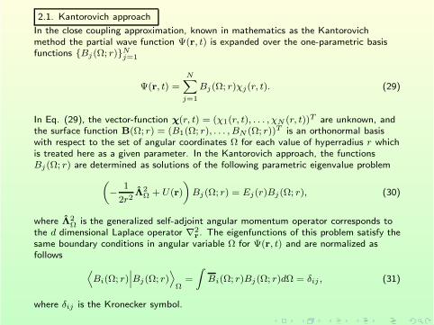
2.1. Kantorovich approach

In the close coupling approximation, known in mathematics as the Kantorovichmethod the partial wave function Ψ(r, t) is expanded over the one-parametric basisfunctions Bj(Ω; r)N

j=1

Ψ(r, t) =NX

j=1

Bj(Ω; r)χj(r, t). (29)

In Eq. (29), the vector-function χ(r, t) = (χ1(r, t), . . . , χN (r, t))T are unknown, andthe surface function B(Ω; r) = (B1(Ω; r), . . . , BN (Ω; r))T is an orthonormal basiswith respect to the set of angular coordinates Ω for each value of hyperradius r whichis treated here as a given parameter. In the Kantorovich approach, the functionsBj(Ω; r) are determined as solutions of the following parametric eigenvalue problem

„

− 1

2r2Λ2

Ω + U(r)

«

Bj(Ω; r) = Ej(r)Bj(Ω; r), (30)

where Λ2Ω is the generalized self-adjoint angular momentum operator corresponds to

the d dimensional Laplace operator ∇2r. The eigenfunctions of this problem satisfy the

same boundary conditions in angular variable Ω for Ψ(r, t) and are normalized asfollows

D

Bi(Ω; r)˛

˛

˛Bj(Ω; r)E

Ω=

Z

Bi(Ω; r)Bj(Ω; r)dΩ = δij , (31)

where δij is the Kronecker symbol.

After minimizing the Rayleigh-Ritz variational functional, and using the expansion (29)the equation (24) is reduced to a finite set of N ordinary second-order differentialequations

ı I∂χ(r, t)

∂t= H(r, t)χ(r, t), χ(r, t0) = χ0(r), (32)

with

H(r, t) = − 1

2rd−1

∂

∂rrd−1I

∂

∂r+ V(r, t) + Q(r)

∂

∂r+

1

rd−1

∂rd−1Q(r)

∂r. (33)

Here I, V(r, t) and Q(r) are matrices of dimension N ×N whose elements are givenby the relation

Vij(r, t) = Vji(r, t) =Ei(r) + Ej(r)

2δij +

1

2

fi

∂Bi(Ω; r)

∂r

˛

˛

˛

˛

∂Bj(Ω; r)

∂r

fl

Ω

+D

Bi(Ω; r)˛

˛

˛f(r, t)˛

˛

˛Bj(Ω; r)E

Ω, Iij = δij , (34)

Qij(r) = −Qji(r) = −1

2

fi

Bi(Ω; r)

˛

˛

˛

˛

∂Bj(Ω; r)

∂r

fl

Ω

.

In this case we obtain the finite N ×N matrix operator-difference scheme forunknown vector-functions χ(r, t)

A(M)k → A

(M)k , A

(M)k,ij =

D

Bi(Ω; r)˛

˛

˛A(M)k

˛

˛

˛Bj(Ω; r)E

Ω, (35)

S(M)k → S

(M)k , S

(M)k,ij =

D

Bi(Ω; r)˛

˛

˛S(M)k

˛

˛

˛Bj(Ω; r)E

Ω,

I → I, Iij = δij .

2.2. High-order approximation of the finite-element method

To solve problem (32) on the time grid Ωτ [t0, T ], the boundary conditions andnormalization condition with respect to the space variable r on an infinite interval arereplaced with appropriate conditions on a finite interval Ωr [rmin, rmax]. Then, at eachk-th step of the time grid Ωτ [t0, T ], we consider the discrete representation of solution

χ(r, tk) to problem (32) with the help of FEM on the grid Ωph = r0 = rmin,

rj = rj−1 + hj , rn = rmax in the form of a finite sum of local functions N(r)

χµ(r, tk) =

npX

l=0

χlµ(tk)Np

l (r), µ = 1, . . . , N, (36)

where χlµ(tk) are node values of the unknown function χµ(r, tk), with respect to

which the initial problem is numerically solved. The local functions Npl (r) are

piecewise continuous polynomials of order p equal to one at one of the nodes rµ and

zero at the other nodes of the grid Ωph; i.e., Np

l (rν) = δlν , l, ν = 0, . . . , np. The

coefficients χlµ(tk) are formally related to the values of the vector χµ(r, tk) of the

problem at the Lagrangian node points

rpj,i = rj−1 +

hj

pi, hj = rj − rj−1, i = 0, p, (37)

by the relations χlµ(tk) ≡ χl

µ(rpj,i, tk), l = i+ p(j − 1).

Substituting (36) into matrix operator-difference scheme, multiplying it from the left

by Npl (r) and integrating over the interval Ωr [rmin, rmax] considering scheme is

reduced to a system algebraic equations for˘

χlµ(rp

j,i, tk)npl=0

¯N

µ=1at given M

A(M)k → A

pk, Ap

k,ij = Apk,ji =

Z rmax

rmin

Npi (r)A

(M)k Np

j (r)rd−1dr, (38)

S(M)k → S

pk, Sp

k,ij = Spk,ji =

Z rmax

rmin

Npi (r)S

(M)k Np

j (r)rd−1dr,

I → Bp, Bpij = Bp

ji =

Z rmax

rmin

Npi (r) INp

j (r)rd−1dr.

3. Numerical tests

3.1. One dimensional modelThe TDSE for a one-dimensional harmonic oscillator with an explicitly time-dependentfrequency in the finite time interval t ∈ [0, T ] has the form

H(x, t) = −1

2

d2

dx2+ω2(t)x2

2, ψ0(x) = 4

r

1

πexp

„

−1

2(x−

√2)2«

, (39)

with ω2(t) = 4 − 3 exp(−t) 8. The exact solution of Eq. (39) reads

ψext(x, t) = 4

r

1

πexp

`

−X(t)x2 + 2Y (t)x − Z(t)´

, (40)

where the functions X(t), Y (t) and Z(t) satisfy to the Cauchy problem

ıd

dtX(t) = 2X2(t) − ω2(t)

2, X(0) =

1

2,

ıd

dtY (t) = 2X(t)Y (t), Y (0) =

√2

2, (41)

ıd

dtZ(t) = −X(t) + 2Y 2(t), Z(0) = 1.

8Puzynin I V, Selin A V and Vinitsky S I 1999 Comput. Phys. Commun. 123 1–6

To approximate the solution ψ(x, t) in the variable x, we used the finite element grid

Ωx[xmin, xmax] = xmin = −10, (100), xmax = 10 and time step τ = .9765625e− 2,where the number in the brackets denotes the number of finite element in theintervals. Between each two nodes we apply the Lagrange interpolation polynomials tothe p = 8 order. To analyze the convergence on a sequence of three double-crowdingtime grids, we define the auxiliary time dependent discrepancy functions

Er2(t, j) =

Z xmax

xmin

|ψ(x, t) − ψτj (x, t)|2dx, (42)

and the Runge coefficient

β(t) = log2

˛

˛

˛

˛

Er(t, 1) − Er(t, 2)

Er(t, 2) − Er(t, 3)

˛

˛

˛

˛

, (43)

where ψτj (x, t) are the numerical solutions with the time step τj = τ/2j−1. For thefunction ψ(x, t) one can use the numerical solution with the time step τ4 = τ/8.Hence, we obtain the numerical estimates for the convergence order of the numericalscheme, that strongly correspond to theoretical ones β(t) ≡ βM (t) ≈ 2M .

1 2 3 4 5 6 7 8 9 10

1E-4

1E-3

0,01

0,1

Er(t,1)

Er(t,2)

Er(t,3)

=9.765625e-3, M=1, (t)=1.99

Er(

t,j)

t

1 2 3 4 5 6 7 8 9 10

1E-9

1E-8

1E-7

1E-6

1E-5

1E-4

Er(t,1)

Er(t,2)

Er(t,3)

=9.765625e-3, M=2, (t)=3.99

Er(

t,j)

t

1 2 3 4 5 6 7 8 9 10

1E-14

1E-13

1E-12

1E-11

1E-10

1E-9

1E-8

1E-7

Er(t,1)

Er(t,2)

Er(t,3)

=9.765625e-3, M=3, (t)=5.99

Er(

t,j)

t

Figure: Values of discrepancy functions Er(t, j) for j = 1, 2, 3 and M = 1, 2, 3.

3.2. Two dimensional modelThe TDSE for a two-dimensional oscillator (or a charged particle in a constantuniform magnetic field) in the external governing electric field with the componentsE1 (t) and E2 (t) in the finite time interval t ∈ (0, T ] has the form

ı∂

∂tφ(x1, y1, t) =−1

2

„

∂2

∂x21

+∂2

∂y21

«

φ(x1, y1, t) +ıω

2

„

x1∂

∂y1− y1

∂

∂x1

«

φ(x1, y1, t)

+ω2

8(x2

1 + y21)φ(x1, y1, t) − (x1E1(t) + y1E2(t))φ(x1 , y1, t). (44)

The transformation to a rotated coordinate system with frequency ω/2

x1 = x cos

„

ωt

2

«

+ y sin

„

ωt

2

«

, y1 = y cos

„

ωt

2

«

− x sin

„

ωt

2

«

, (45)

and x = r cos(θ), y = r sin(θ), leads to the following equation

ı∂

∂tφ(r, θ, t) = −1

2

„

1

r

∂

∂rr∂

∂r+

1

r2∂2

∂θ2

«

φ(r, θ, t) (46)

+ω2r2

8φ(r, θ, t) + r(f1(t) cos(θ) + f2(t) sin(θ))φ(r, θ, t),

f1(t) = −E1(t) cos

„

ωt

2

«

+ E2(t) sin

„

ωt

2

«

, (47)

f2(t) = −E1(t) sin

„

ωt

2

«

− E2(t) cos

„

ωt

2

«

.

Using the Galerkin projection of solutions by means of the basis of the angularfunctions Bj(θ)

φ(r, θ, t) =NX

j=1

Bj(θ)χj(r, t), (48)

B1(θ) =1√2π, B2j(θ) =

sin(jθ)√π

, B2j+1(θ) =cos(jθ)√

π, j ≥ 1, (49)

we arrive at the matrix equation (32) for unknown coefficients χj(r, t)Nj=1 in the

interval t ∈ [0, T ]. The initial functions χj(r, t) at t = 0 (in the casef1(0) = f2(0) = 0) are chosen in the form

χ1(r, 0) =√ω exp

„

−1

4ωr2

«

, χj(r, 0) ≡ 0, j ≥ 2. (50)

Note that, this problem has an exact solution for a partial choice of the field

Ej(t) = aj sin(ωjt) (51)

which that provides a good test example to examine efficiency of numerical algorithmsand a rate of convergence of the projection by a number N of radial equations and bytime T . The needed projections of an exact solution to the radial ones have the form

χextj (r, t) =

Z 2π

0Bj(θ)φext(r, θ, t)dθ. (52)

We choose ω = 4π, ω1 = 3π, ω2 = 5π, a1 = 24 and a2 = 9. For these parametersthe absolute value of the solution φ(x, y, t) is should be periodically with periodT = 2, i.e., |φ(x, y, t)| = |φ(x, y, t+ T )|.To approximate the solution χj(r, t) in the variable r, we used the finite element grid

Ωr [rmin, rmax] = rmin = 0, (120), 1.5, (60), rmax = 4 and time step τ = 0.00625,where the number in the brackets denotes the number of finite element in the intervals.Between each two nodes we apply the Lagrange interpolation polynomials to thep = 8 order. To analyze the convergence on a sequence of three double-crowding timegrids, we define the auxiliary time dependent discrepancy functions analogy to (42)

Er2(t, j) =NX

ν=1

Z rmax

0|[χν(r, t) − χ

τjν (r, t)]|2rdr, j = 1, 2, 3, (53)

where χτjν (r, t) are the numerical solutions with the time step τj = τ/2j−1. For the

function χν(r, t) one can use the numerical solution with the time step τ4 = τ/8.

Table: The test results of the discrepancy functions Er(t, j) (j = 1, 2, 3) for the approximationsM = 1, 2, 3. Here number of the used differential equations N = 30, time step τ = 0.00625,and t is some times.

M=1t Er(t, 1) Er(t, 2) Er(t, 3) β1(t)

0.4 0.7399(-02) 0.1777(-02) 0.3562(-03) 1.9840.8 0.4054(-01) 0.9773(-02) 0.1960(-02) 1.9771.2 0.7351(-01) 0.1777(-01) 0.3566(-02) 1.9721.6 0.7630(-01) 0.1844(-01) 0.3700(-02) 1.9732.0 0.8103(-01) 0.1957(-01) 0.3925(-02) 1.974

M=2t Er(t, 1) Er(t, 2) Er(t, 3) β2(t)

0.4 0.6811(-05) 0.4261(-06) 0.2509(-07) 3.9930.8 0.6156(-04) 0.3858(-05) 0.2273(-06) 3.9911.2 0.1228(-03) 0.7700(-05) 0.4537(-06) 3.9891.6 0.1256(-03) 0.7882(-05) 0.4645(-06) 3.9882.0 0.1313(-03) 0.8254(-05) 0.4866(-06) 3.986

M=3t Er(t, 1) Er(t, 2) Er(t, 3) β3(t)

0.4 0.5064(-08) 0.9193(-10) 0.3799(-10) 6.5260.8 0.6363(-07) 0.1008(-08) 0.6168(-10) 6.0471.2 0.1438(-06) 0.2262(-08) 0.7341(-10) 6.0151.6 0.1723(-06) 0.2719(-08) 0.8136(-10) 6.0072.0 0.2634(-06) 0.4209(-08) 0.1039(-09) 5.981

approx: t= 1.200

–1.5–1–0.50

0.51

1.5

x–1.5–1

–0.500.5

11.5

y

0.5

1

1.5

approx: t= 2.000

–1.5–1–0.50

0.51

1.5

x–1.5–1

–0.500.5

11.5

y

0.5

1

1.5

difference: t= 1.200

–1.5–1–0.50

0.51

1.5

x–1.5–1

–0.500.5

11.5

y

0.0010.0020.0030.004

difference: t= 2.000

–1.5–1–0.50

0.51

1.5

x–1.5–1

–0.500.5

11.5

y

0.0010.0020.0030.004

Figure: The absolute values of the numerical solution |φ(x, y, t)| and difference|φext(x, y, t) − φ(x, y, t)| at t = 1.2 and t = 2. Here N = 30, τ4 = τ/8 = 0.00078125 andM = 3.

3.3. Three dimensional modelAs known, the δ-shaped pulses are a widely used approximation for electric-field pulsesthat are much shorter than the classical orbital period. The Hamiltonian of the kickedhydrogen atom in a magnetic field reads

H = H0 + Vext, H0 = −1

2∆r − 1

r+β2r2

8sin2(θ), Vext = rF

SX

k=1

δ(t − kT ), (54)

where S is the number of kicks applied, T its period, β = B0/B is a dimensionlessparameter which determines the field strength B, and F = (0, 0, F ) is the externalfield. Between the pulses the wave packet evolves according to the TDSE

ı∂ψ(r, t)

∂t= H0ψ(r, t). (55)

We use following formula for calculation of wave function ψ(r, sT+) directly after thepulse t = sT+

ψ(r, sT+) = exp (−ı rF)ψ(r, sT−). (56)

via the wave function ψ(r, sT−) immediately before the pulse.

Using the Kantorovich expansion of solutions by means of the basis functions Bj(θ; r)

ψ(r, t) =exp(ımϕ)√

2π

NX

j=1

Bj(θ; r)χj(r, t). (57)

The functions Bj(η = cos(θ); r) are determined as solutions of the followingparametric eigenvalue problem 9 10

„

− 1

2r2

„

∂

∂η(1 − η2)

∂

∂η− m2

1 − η2

«

− 1

r+β2r2

8(1 − η2)

«

Bj(η; r) (58)

= Ej(r)Bj (η; r).

9Chuluunbaatar O, Gusev A A, Gerdt V P, Rostovtsev V A, Vinitsky S I, Abrashkevich A G, Kaschiev M S andSerov V V 2007 accepted in Comput. Phys. Commun. doi:10.1016/j.cpc.2007.09.005.

10Chuluunbaatar O, Gusev A A, Derbov V L, Kaschiev M S, Serov V V, Melnikov L A and Vinitsky S I 2007 J.Phys. A 40 11485–11524.

β = 0; F = 0.002; T ≡ Tn=9 = 5357 : (59)

Pn(t) =

n−1X

l=0

|〈nl0|ψ(r, t)〉|2 the probability function : (60)

C(t) = |〈ψ(r, t)|ψ0(r)〉| the autocorrelation function : (61)

|ψ0(r)〉 = |n = 9k = 0m = 0〉11 : (62)

r → r/n; t→ t/n2; T = Tn = Tn/n2 ∼ 66 : (63)

ψ

Figure: The dynamics of physical quantities of a kicked hydrogen atom.

11Klews M and Schweizer W 2001 Phys. Rev. A, 64 053403-1-053403-5.

β = 0.1472e − 4; F = 0.002; T ≡ Tn=9 = 5357 : (64)

Table: The eigenvalues Ecalc calculated by the code KANTBP 12 of the magneticstates n = 9, v,m = 0, δEcalc = (Ecalc − E(0))/β2 corresponds to the first order

corrections E(1)pt by of a perturbation calculation Ept = E(0) + β2E

(1)pt . Below, the

factor x in the brackets means (x) ≡ 10x.

v Ecalc E0 δEcalc E1pt

0 -6.172 798(-3) -6.172 839 (-3) 1529.11 1529.161 -6.172 797(-3) -6.172 839 (-3) 1545.01 1545.042 -6.172 747(-3) -6.172 839 (-3) 3384.07 3384.103 -6.172 728(-3) -6.172 839 (-3) 4080.42 4080.474 -6.172 689(-3) -6.172 839 (-3) 5536.15 5536.385 -6.172 641(-3) -6.172 839 (-3) 7315.02 7315.336 -6.172 582(-3) -6.172 839 (-3) 9476.34 9476.837 -6.172 514(-3) -6.172 839 (-3) 12006.50 12007.138 -6.172 435(-3) -6.172 839 (-3) 14902.72 14903.51

12Chuluunbaatar O, Gusev A A, Abrashkevich A G, Amaya-Tapia A, Kaschiev M S, Larsen S Y and Vinitsky S I2007 Comput. Phys. Commun. 177 649–675.

900+1

–200

–100

0

100

200

x–200 –100 0 100z

0.0060.0040.002

0–0.002–0.004–0.006

980+1

–200

–100

0

100

200

x–200 –100 0 100z

0.0060.0040.002

0–0.002–0.004–0.006

Figure: The three dimensional plots of the normalized even wave functions in zx planeof states |n = 9v = 0m = 0〉 and |n = 9v = 8m = 0〉13.

13Chuluunbaatar O, Gusev A A, Derbov V L, Kaschiev M S, Serov V V, Melnikov L A and Vinitsky S I 2007 J.Phys. A 40 11485–11524.

|ψ0(r)〉 = |n = 9v = 0m = 0〉 |ψ0(r)〉 = |n = 9v = 8m = 0〉

ψ

!

ψ

!Figure: The dynamics of physical quantities of a kicked hydrogen atom in the magnetic field.

4. ConclusionsWe have presented a new computational approach to solve the TDSE, in which partial(unitary) splitting of evolution operator and the FEM are combined togethereffectively. Especially, to realize our approach in an explicit form, we have derived thesecond-, fourth-, and sixth-order approximations with respect to time step. Severalnumerical results have been also given which turn out to agree with the theoreticalones to a good extent.