1

Multi-Echelon Models for Repairable Items: A Review

Angel Díaz IESA

av. IESA, San Bernardino Caracas 1010, Venezuela

582-521533 582-524247 (fax)

Michael C. Fu*

College of Business and Management Institute for Systems Research

University of Maryland College Park, MD 20742 mfu@bmgtmail.umd.edu

(301) 405-2241 (301) 314-9157 (fax)

Abstract We review multi-echelon inventory models for repairable items. Such models have been widely applied to the management of critical spare parts for military equipment for around three decades, but the application to manufacturing and service industries seems to be much less documented. We feel that the appropriate use of models in the management of spare parts for heavily utilized equipment in industry can result in significant cost savings, in particular in those settings where repair facilities are resource constrained. In our review, we provide a strategic framework for making these decisions, place the modeling problem in the broader context of inventory control, and review the prominent models in the literature under a unified setting, highlighting some key relationships. We concentrate on describing those models which we feel are most applicable for practical application, revisiting in detail the Multi-Echelon Technique for Recoverable Item Control (METRIC) model and its variations, and then discussing a variety of more general queueing models. We then discuss the components which we feel must be addressed in the models in order to apply them practically to industrial settings. * corresponding author; supported in part under NSF Grant D CDR-8803012.

2

Keywords: Multi-Echelon Inventory Control, Spare Parts Management, Maintenance

3

Multi-Echelon Models for Repairable Items: A Review 1. Introduction Inventories represent about one-third of all assets of a typical company in the United States, with the total value of capital tied up in inventories around $1.1 trillion in 1992, representing over 20% of the GNP (Economic Report of the President 1993). Of these inventories, repairable items — those items that can be repaired following a breakdown or failure — are of particular importance for manufacturing and service industries that are characterized by heavily utilized, relatively expensive, equipment. Examples of these include continuous chemical or petrochemical processes, mass transit systems, and the military. To insure continuity of operations, an ample supply of spare parts must be maintained; however, this must be traded off with the cost of tying up capital in non-revenue-generating spare parts inventories. In the context of standard inventory control, stockouts can lead to unavailability of equipment, translating to a loss of service or production capability, whereas spare parts inventories incur holding costs. The magnitude of these economical implications are such that in the United States military world alone, repairable items represented about $10 billion in 1976 (Nahmias 1981), and about $30 billion in 1994 (O’Malley 1994). Systems for repairable items usually assume the configuration depicted in Figure 1. Spare parts that can be economically repaired are stocked in locations known as bases, using military terminology. When a failure occurs, the defective part is removed, exchanged for a fresh part taken from the base stock (if such a spare part is available) and sent to a repair facility known as the depot, where it is repaired and held in stock, to be eventually sent down to the bases to cover another part used in a repair. Parts are thus subject to cycles and not freshly brought from the outside (assuming that all items can be repaired). Base level is considered one echelon of inventory control, and depot level is considered another echelon, hence the term multi-echelon inventory control. The basic model allows spare parts to be stocked at either echelon — with exchange of parts between echelons but not within the same echelon — and all repairs are done at the depot echelon. Important practical variations of this basic model include allowing some of the following: repairs at both echelons, lateral transshipment within an echelon (e.g., between bases), and total failures, modeled as a proportion of the failures being classified as non-repairable. The objective of this paper is to provide a current review of multi-echelon inventory models for repairable items, with emphasis on the applicability of the models. We are in particular motivated by resource-constrained industrial settings — either manufacturing

4

or service — which seems to have received much less attention in the literature than military applications, where repair resources are assumed to be plentiful. We hope to target both practitioners with a vested interest in spare parts management and academics with little previous exposure to the area of multi-echelon repairable item inventory models. To this end, we have included the following: • a simple framework for establishing the relative importance of repairable items in

a given manufacturing or service industry; • a classification of multi-echelon inventory models for repairable items in the

context of the general inventory control literature and terminology; • a concise summary presentation of the key components and relationships involved

in analyzing multi-echelon repairable item models; • a detailed discussion of the Multi-Echelon Technique for Recoverable Item

Control (METRIC) model, on which most of the prevailing models used in military practice are based;

• an overview of various queueing models and a discussion of their applicability; • a more forward-looking discussion of the various model assumptions which can

be critical in applications, such as the use of priority processing for repair and distribution, pointing the need for further research.

We also view our paper as updating and complementing the two excellent older reviews on this subject by Clark (1972) and Nahmias (1981). Also of note is the chapter by Axsäter (1993), which concentrates mainly on a more general multi-echelon setting — not specifically repairable items — and does not include queueing models. Our attempt is to view all the repairable item inventory models, both METRIC and queueing-based, from a single perspective, instead of as disparate approaches to the same problem. The rest of the paper is organized as follows. In Section 2, recognizing that the use of multi-echelon inventory models must be justified by potential gains in operations, we present an operations strategy framework for determining the relevance of repairable items in inventory control. In Section 3 we place multi-echelon repairable item inventory models in context by providing a broad overview and classification of inventory models in general. Section 4 is dedicated to reviewing the major classes of models for repairable items: the METRIC model and its various extensions and successors, and queueing network models. Through the use of a simple example, we introduce the key components required by any multi-echelon repairable item inventory model: a characterization of queueing effects and two superposition of processes to determine backorders. Section 5 discusses the assumptions in the prevailing models deemed most critical to address for application to industrial settings, suggesting directions for further research.

5

2. The Strategic Importance of Repairable Item Inventories In practice, the use of multi-echelon inventory models for the management of repairable item stock must be driven by a need to control the inventory costs of such items, i.e., if spare parts are extremely cheap and/or failures relatively infrequent, then there is probably little need to engage in any sophisticated form of inventory control, aside from bookkeeping. In brief, the relative importance of repairable items depends on the manufacturing or service type of operation in which they are used. In this section, we outline two operations strategies frameworks, one for manufacturing and one for services, useful for determining across different industries the need for the various models contained in this review.

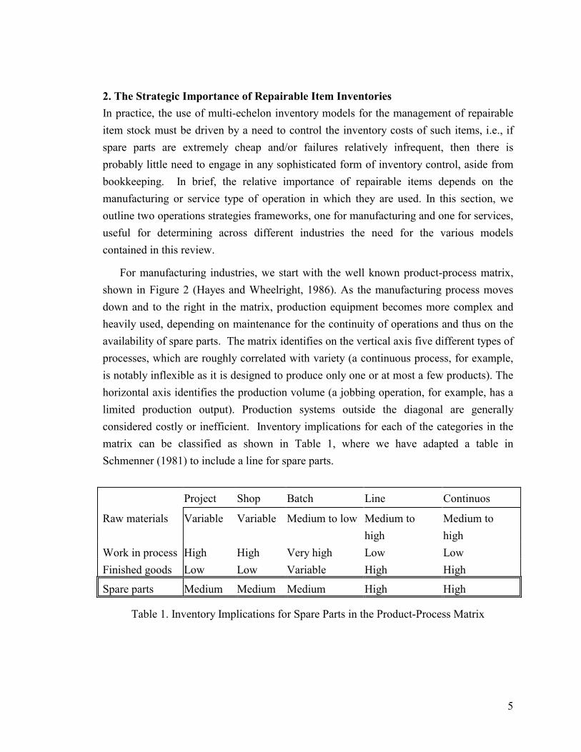
For manufacturing industries, we start with the well known product-process matrix, shown in Figure 2 (Hayes and Wheelright, 1986). As the manufacturing process moves down and to the right in the matrix, production equipment becomes more complex and heavily used, depending on maintenance for the continuity of operations and thus on the availability of spare parts. The matrix identifies on the vertical axis five different types of processes, which are roughly correlated with variety (a continuous process, for example, is notably inflexible as it is designed to produce only one or at most a few products). The horizontal axis identifies the production volume (a jobbing operation, for example, has a limited production output). Production systems outside the diagonal are generally considered costly or inefficient. Inventory implications for each of the categories in the matrix can be classified as shown in Table 1, where we have adapted a table in Schmenner (1981) to include a line for spare parts.

Project Shop Batch Line Continuos

Raw materials Variable Variable Medium to low Medium to high

Medium to high

Work in process High High Very high Low Low Finished goods Low Low Variable High High

Spare parts Medium Medium Medium High High

Table 1. Inventory Implications for Spare Parts in the Product-Process Matrix

6

Thus, in manufacturing, we feel that the management of spare parts inventory is fairly critical for all types of industries, but in particular for those with high equipment utilization and expensive machinery.

For service operations, Figure 3 gives an analogous matrix (Schmenner 1986), including the inventory implications annotated for each entry. The vertical axis identifies intensity of equipment use (defined as the value of the equipment divided by the yearly payroll), while the horizontal axis identifies the degree to which the service is adapted to the customer needs or wishes. For service organizations that depend heavily on equipment utilization — the upper half region of the service matrix — maintenance and spare parts are critical. For example, in both the Caracas subway system in Venezuela and the United States Air Force, repairable items represent almost 2/3 of all inventory value. In addition, Schmenner (1986) identifies a trend of services to reduce costs by moving towards the upper left quadrant (service factories), where managing repairable item inventories is particularly critical.

In summary, there are many industries in both manufacturing and services where there are opportunities for cost savings by engaging in more efficient management of spare parts inventories, and the trend in both sectors is such that it is likely to become even more critical. For example, in manufacturing, the reduction of product-related inventories (raw materials, work-in-process, and finished product) being undertaken in both just-in-time and traditional materials requirements planning (MRP) environments will require increased equipment reliability for continuity of operations. 3. Classification of Inventory Models In this section, we provide a concise general taxonomy of the most commonly encountered inventory models in practice and in the inventory literature. A summary of the classification is presented in Figure 4. For historical background, classic books dedicated to inventory management include Arrow, Karlin, and Scarf (1958, 1962), Hadley and Whitin (1963), and Scarf, Gilford, and Shelley (1963). Directly relevant to this review, the edited book by Schwarz (1981) contains a compendium of 16 state-of-the-art (at that time) research papers on multi-level inventory models, including three on repairable items. Foremost is Nahmias (1981), still the most comprehensive review published in this field, which discusses a two-step approach: first characterize the performance of the system using a measure such as expected backorders and then search systematically among combinations of spares at different levels until an optimal solution is found. Two other papers, by Clark (1981) and by Demmy and Presutti (1981) analyze

7

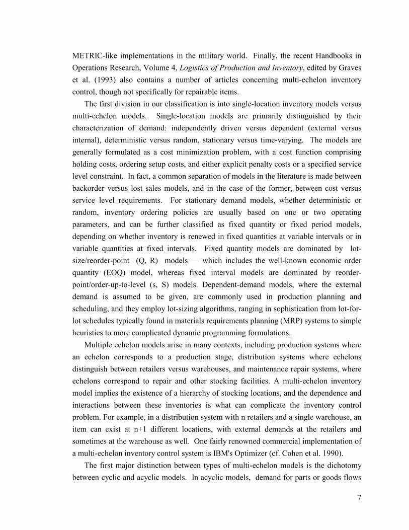
METRIC-like implementations in the military world. Finally, the recent Handbooks in Operations Research, Volume 4, Logistics of Production and Inventory, edited by Graves et al. (1993) also contains a number of articles concerning multi-echelon inventory control, though not specifically for repairable items. The first division in our classification is into single-location inventory models versus multi-echelon models. Single-location models are primarily distinguished by their characterization of demand: independently driven versus dependent (external versus internal), deterministic versus random, stationary versus time-varying. The models are generally formulated as a cost minimization problem, with a cost function comprising holding costs, ordering setup costs, and either explicit penalty costs or a specified service level constraint. In fact, a common separation of models in the literature is made between backorder versus lost sales models, and in the case of the former, between cost versus service level requirements. For stationary demand models, whether deterministic or random, inventory ordering policies are usually based on one or two operating parameters, and can be further classified as fixed quantity or fixed period models, depending on whether inventory is renewed in fixed quantities at variable intervals or in variable quantities at fixed intervals. Fixed quantity models are dominated by lot-size/reorder-point (Q, R) models — which includes the well-known economic order quantity (EOQ) model, whereas fixed interval models are dominated by reorder-point/order-up-to-level (s, S) models. Dependent-demand models, where the external demand is assumed to be given, are commonly used in production planning and scheduling, and they employ lot-sizing algorithms, ranging in sophistication from lot-for-lot schedules typically found in materials requirements planning (MRP) systems to simple heuristics to more complicated dynamic programming formulations. Multiple echelon models arise in many contexts, including production systems where an echelon corresponds to a production stage, distribution systems where echelons distinguish between retailers versus warehouses, and maintenance repair systems, where echelons correspond to repair and other stocking facilities. A multi-echelon inventory model implies the existence of a hierarchy of stocking locations, and the dependence and interactions between these inventories is what can complicate the inventory control problem. For example, in a distribution system with n retailers and a single warehouse, an item can exist at n+1 different locations, with external demands at the retailers and sometimes at the warehouse as well. One fairly renowned commercial implementation of a multi-echelon inventory control system is IBM's Optimizer (cf. Cohen et al. 1990). The first major distinction between types of multi-echelon models is the dichotomy between cyclic and acyclic models. In acyclic models, demand for parts or goods flows

8

in only one direction. These inventory items are sometimes referred to as consumable items, as opposed to repairable items. Cyclic models are those in which inventory flows through the system as demanded by the different locations, so inventory is neither lost nor produced, though it may undergo some sort of transformation, as in repairs and failures in our context. Thus, in repairable item multi-echelon models, failure and repair events drive the “demand” in the system. We note that the distinction between acyclic and cyclic inventory models bears a strong resemblance to that of open and closed queueing networks. Production and distribution models fall into the class of acyclic multi-echelon models. The first important work in this area was done by Clark and Scarf (1960, 1962). Acyclic models can be classified, as in the single-location case, as time-varying dependent or independent stationary demand models. Dependent-demand models obtain pyramidal requirements aggregating known demands at the different echelons in a hierarchical form, e.g., as in MRP systems for production systems or DRP (Distribution Resources Planning) for distribution; see also Muckstadt and Roundy (1993) for an updated summary. For independent demand models, there are two approaches. One obvious approach taken by many inventory models is to decompose the system by treating each location as independent and thereby applying techniques for the single-location model. Usually, such local optimization leads to a suboptimal solution for the entire system. On the other hand, there is a lot of academic research tackling the more accurate approach, at the cost of complexity, that includes the interactions between echelons. Some discussion of this can by found in Federgruen (1993). In this review, we are concerned with the cyclic type of multi-echelon models, in particular models which include repairable item inventory. Replenishment is usually either periodic or based on a re-order point. Again, determination of the operating parameters could either be done based on local optimization or on a systemwide analysis. In addition, the operating policy itself could depend on only local information (e.g., only the stock variables at the location) or it could incorporate systemwide state variables. The general replenishment problem would involve determining a batch replenishment policy, similar to either a (Q,R) policy or (s,S) policy in the single-location case. However, the focus of this review is on low-demand, high-cost, and relatively low order setup cost items, in which case one-for-one replenishment is assumed. Intuitively, the EOQ tends to a size of one in this case. Thus, a part is ordered every time it is used, and local inventory control is determined by a single value, the target base-stock level. This is

9

sometimes written as a continuous review (S-1, S) policy, equivalent to the (Q,R) model with lot size Q=1 and R=S-1. The advantages of multi-echelon models for low demand items over their single-location counterparts have been established by Muckstadt and Thomas (1980). The one-for-one replenishment policy considerably simplifies the models. The most influential model by far has been the Multi-Echelon Technique for Recoverable Item Control (METRIC), developed by Sherbrooke (1968) while working at the Rand Corporation, and extensively used in the military world. Aside from the seminal Sherbrooke (1968) paper that introduces METRIC, other important advances include Feeney and Sherbrooke (1966) which shows that Palm's theorem still applies under compound Poisson demand, Simon (1971) which analyzes stationary properties for a simple two-echelon system, Muckstadt (1973) which introduces multi-indenture problems, Allen and d'Esopo (1968) which provides a (Q, R) formula for a system with Poisson failures and constant repair times, and Fox and Landi (1970) which introduces the use of Lagrangean multipliers in place of marginal analysis for optimization. Sherbrooke's work is interesting from a practical perspective for two reasons. First, he proposes exchange curves of system availability versus investment value of spares, rather than offering a single “optimal value”. Availability values are obtained from the performance characterization of backorders at the bases via the METRIC model. Secondly, he allocates spare parts in the system on a global basis, since the METRIC model considers all locations simultaneously in the performance analysis. Muckstadt and Thomas (1980) show that even simple multi-echelon approaches like METRIC will yield better results than naive local optimization. Probably the most important “extension” of the METRIC model is Graves (1985), who developed a simple, easy-to-understand framework that in some sense superseded METRIC, and included some approximations that outperformed METRIC. The other class of models considered important in this review are queueing network models for repairable items, which were developed to relax some assumptions that may be unrealistic in application (for example, infinite repair channels and infinite working item population, assumed by METRIC), mainly by Gross et al. (1978, 1983, 1987, 1993) and by Albright et al. (1988, 1989, 1993). Finally, simulation can also be used to obtain results under more “real-life” conditions (e.g., Bier and Tjelle 1994). To summarize by putting into the general inventory control context, this review focuses on multi-echelon inventory system models with the following characteristics: • cyclic inventory (repairable items); • stationary, random demand; • continuous review;

10

• full backlogging; • one-for-one replenishment ordering policy. In the next section, we will discuss the actual models, all under a common framework.

4. Multi-echelon Models for Repairable Items In this section, we present the key relationships that form the basis for analyzing multi-echelon models for repairable items, and then discuss actual models which allow one to determine the quantities in these relationships and hence calculate system performance measures of interest. In particular, the overall analysis follows these basic steps: 1) determine the distributions of the parts population throughout the various elements of the system; 2) combine the distributions to determine appropriate backorder distributions; 3) determine availability from the backorder distributions. Our concentration will be on the first two steps. 4.1 The Basic Model and Key Relationships We will introduce the key components in the models for repairable items with a simple example. We consider a system comprising a single base and a single depot with a target level of s0 spares at the depot and a target level of s1 spares at the base. This system can be represented as a network of elements, as shown in Figure 5: • a set of working parts at the base “field” (e.g., in the factory or service operation), • a base-to-repair facility transportation pipeline of failed parts (the in-pipeline), • a repair facility of failed parts to be repaired, • a depot storage facility stocking spare parts, • a depot-to-base transportation pipeline of parts (the out-pipeline), • a base storage facility stocking spare parts.

The repair facility and transportation pipelines are represented schematically by queues — as parts may experience delays in requests for repairs or transportation — and the depot and base by physical inventories. Part movement in the system occurs in three modes:

(1) a part failure activates three movements:

(i) the failed part moves from the field to the base-to-repair transportation pipeline, (ii) a part, if one is available, moves from depot stock to the depot-to-base transportation pipeline; if no part is available, a backorder is placed at the depot, and

11

(iii) a part, if one is available, moves from base stock to the field; if no part is available, a backorder is placed at the base.

(2) a part repair is completed — the part is moved from the repair facility to the depot storage.

(3) transportation of a part is completed (two types): the part is

(i) placed into base stock, or

(ii) arrives at the repair facility.

Thus, as described in the introduction, parts cycle through the system after a failure by being moved to the repair facility, repaired and then held in stock at the depot to be eventually sent to the base to cover a failure. Let Ni(t) denote the number of parts in location i at time t, where i=0 represents the field operations, i=1 represents the in-pipeline, i=2 represents the repair facility, i=3 represents the depot, i=4 represents the out-pipeline, and i=5 represents is the base. We allow Ni(t)<0 for i=0, i=3 and i=5, indicating a backordered condition in the field, at the depot, or at the base, respectively, i.e., N0(t), N3(t), and N5(t) can be thought of as the inventory levels in the usual inventory control parlance, which as we shall see are derived from the other three processes. Recall that the variables s0 and si denote the target number of spares at the depot and the base, respectively. In addition, we will explicitly define the quantities B0(t) and B1(t) to denote the backorder levels at the depot and base, respectively, i.e., B0(t)=N3-(t) and B1(t)=N5-(t), where x-=max(0,–x) is the negative part of x. Then, independent of any assumptions on the failure process, the repair process, or the transportation processes, we have the following key relationships (indicated in the sample path diagram of Figure 6): N1(t)+N2(t)+N3(t) =s0 (1) B0(t) = N3-(t) = [N1(t)+N2(t)-s0]+ (2) N4(t)+N5(t)+B0(t) =s1 (3) B1(t) = N5-(t) = [N4(t)+B0(t)-s1]+ (4) N0(t)+B1(t) =N, (5) where x+=max(0,x) is the positive part of x, and N denotes the total nominal working population of parts. METRIC assumes that N and hence N0(t) is essentially infinite. Under this infinite working parts population assumption the failure rate is a constant value (i.e., independent of the number of working parts), and the system acts essentially like an open network, i.e., we can “cut” the network in Figure 5 at the indicated place. The

12

relationships above can be easily established by looking at the various part movement possibilities specified above, which result in the following changes:

(1) (i) N1(t): +1, N3(t): -1,

(ii) N4(t) or B0(t) : +1, N5(t): -1,

(iii) N0(t) unchanged, or N0(t) : -1 and B1(t): +1,

(2) N2(t): -1, N3(t): +1,

(3) (i) N4(t): -1, N5(t): +1,

(ii) N1(t): -1, N2(t): +1. We illustrate the progression with a simple sample path (trajectories) for the various processes Ni(t). We will take the METRIC standard assumptions of an unlimited working parts population and an uncapacitated repair facility. In this case, without loss of generality, we will assume that the base-to-depot transportation times are instantaneous, so that the in-pipeline will always be empty. Essentially, the times can be subsumed in the repair times under the assumption of unlimited repair capacity. We further assume that a failure occurs each unit of time, a repair take two units of time, and the depot-to-base delivery time is three units of time. Stopping the generation of failures after the second failure takes place (noting that otherwise this system would be unstable in the long run), we have the following sequence of events, where the various trajectories are shown in Figure 7): _ At t=1, a part fails. The failed part is sent from base to repair; another part is sent from

depot to the out-pipeline. _ At t=2, a part fails. The failed part is sent from base to repair; another one is

backordered at the depot. _ At t=3, a part repair is completed. The repaired part goes directly to the out-pipeline, as

there are backorders at the depot. _ At t=4, a part repair is completed and a part shipment arrives at the base from the out-

pipeline. The repaired part is sent to the depot. _ At t=6, the remaining part in the out-pipeline arrives at the base. The shaded areas at repair and in the out-pipeline in Figure 7 represent physical units at that location, while the shaded areas at the base and the depot represent units missing at that location, or outstanding parts, s0-N3(t) and s1-N5(t), respectively. A negative value at the base represents a “hole,” i.e., unavailability of a needed part in the field, while a negative value at the depot represents a unit demanded by a base but not satisfied, i.e., a backorder.

13

The distribution of parts in repair and of outstanding parts at the depot (the shaded areas in Figure 8) are complementary, as reflected by Equation (1), and the backorder distribution at the depot is just the negative part of the distribution of outstanding parts at the depot (N3(t)), as reflected by Equation (2). Figure 9 illustrates Equation (3), where the sum of parts at the pipeline (N4) plus the negative part of outstanding parts at the depot (B0(s0)) gives the outstanding parts at the base. This has a simple intuitive explanation: As parts are not created or destroyed, when a part leaves the base, another is pulled from the depot and put into the pipeline; if no parts are available, a backorders occurs at the depot. Thus, we can see from Figures 8 and 9 how the multi-echelon problem for repairable items can be basically reduced to (i) finding the backorder distribution at the depot, for a given level of spare parts s0, and then (ii) combining this with the distribution of parts in the out-pipeline. We describe some straightforward extensions of this simple model. For multiple bases, a form of Equations (1) and (3) with multiple in-pipelines still apply, but backorders at the depot must be appropriately apportioned to the bases to obtain the distribution of outstanding parts at the bases — corresponding to Equation (4) — and then from these the performance measures, such as fill rate or expected backorders. If the superscripted i represents the corresponding quantities as defined before for base i, then our key equations become the following:

ΣΣΣΣiNi

1(t)+N2(t)+N3(t) =s0 (1’)

B0(t) = N3-(t) = [ΣΣΣΣiNi

1(t)+N2(t)-s0]+ (2)

Ni4(t)+Ni

5(t)+B0(t) =si (3’) Bi

1(t) = Ni5-(t) = [iN4(t)+αiB0(t)-si]+ (4’)

N0(t)+ΣΣΣΣiBi

1(t) =N, (5’)

where αi represents the apportioning of depot backorders to base i. If the allocation of parts to the bases is done strictly on a first-come, first-served basis, the apportioning, αi, is simply proportional to each base demand. In addition, an extension to local repairs can also be easily incorporated. When a proportion of the repairs can take place locally at the base, the number of parts must also be convolved with the distribution of parts in the pipeline. Referring to Figure 5, parts not in the field can be in the in-pipeline; being repaired or waiting in queue at the depot; in stock at the depot; in the out-pipeline; or in stock at the base, represented by N1, N2, N3, N4 and N5, respectively, where we drop the time argument for convenience here, and later to indicate the corresponding steady-state

14

quantities). The distribution of backordered parts at the depot is derived from the sum of N1 and N2, which can then be used to determine the distribution of backordered parts at the bases. In sum, to analyze performance of the system requires the analyses of three primary types of processes: in-pipeline(s), repair, and out-pipeline(s), and then solving two sets of superpositions of processes, per Equations (1) and (3): the first to obtain the distribution of the depot stock inventory level (N3) from the distributions of in-pipeline parts (N1) and parts in repair (N2); and the second to obtain the distribution of the base stock inventory level (N5) from the depot backorder distribution derived from N3 and the distribution of out-pipeline parts (N4). An infinite parts population assumption allows us to basically ignore Equation (5); otherwise, the failure process for N1 is determined through it. Under the assumption of independence of the involved distributions, the superpositions reduce to calculating two convolutions. In the case of multiple bases, the first convolution is obtained from the parts in all in-pipelines, while the second requires decomposing the distribution of backorders at the depot into the bases and then convolving with each base out-pipeline; or alternatively convolving the distribution of backorders with parts in all out-pipelines and then decomposing this into the bases (Graves 1985). In general, the first superposition is treated as a convolution, because the model assumptions lead to independence of the steady-state random variables involved. In METRIC, the second superposition is also treated as a convolution, whereas Graves (1985) derives an exact expression under certain conditions and a better approximation than METRIC for the more general case. The assumption of independent Poisson processes everywhere — as in METRIC— simplifies the analysis considerably, as the superposition of independent Poisson processes is again Poisson.

4.2 The METRIC model We now explicitly describe METRIC in detail. As discussed for the simple two-echelon system with a single depot and multiple bases, the critical assumptions for the METRIC model are the following: _ One-for-one replenishment; _ Poisson failure process; _ Large working parts population; _ Ample repair facilities. or equivalently, repair times independent of the number of parts in repair. In inventory control terminology, the stocking policies at each echelon follow a continuous review base-stock policy with target level si, also known as an (S-1,S) policy where inventory position (on-hand plus on-order) is maintained at S=si. In queueing

15

theory terminology, the system is represented as an open queueing network decomposed as M/G/ / / queues for nodes 1, 2, and 4 (using the Kendall notation for queueing models, where M stands for a Poisson arrival process, G for a general service distribution and for the number of service channels or servers, the population capacity of the system and the size of the working parts population, respectively). Because both 1 and 2 are M/G/ queues, we can combine them into a single node, which we did in the last section for the illustrative example, and is implicit in the METRIC formulation; thus, there is no N1 to consider.

We begin by defining some notation for the model. Let L0 = average repair time at the depot , λ0 = demand rate at the depot (sum of demands at bases, Σλi), W0 = delay due to stockouts at the depot, s0 = spares target level at the depot, N2 = number of parts at repair in the depot, E(B0) = expected number of backorders at the depot. Under the METRIC assumption of ample repair facilities and Poisson demand, N2 also follows a Poisson distribution, with mean λ0L0, so we have

E(B0)= E[(N2-s0)+]=ΣΣΣΣn>s0

(n-s0)(λ0L0)exp(-λ0L0)/n!, (6) and thus the expected delay came be found from Little's law, E(W0)=E(B0)/λ0 (7)

Note that the expected backorder level, and not fill rate — the proportion of demand filled from depot stock, given by P(N2<s) — is used to evaluate performance in METRIC. The rationale for this is that fill rate (the percent of demand filled from on-hand stock) doesn't take into account the time that the item is unavailable, whereas this time is implicit in the average level of backorders. We can now define, analogous to the depot, the following quantities for the bases: Li= replenishment time (depot to base i), Wi = delay due to stockouts at base i, si = spares target level at base i, E(Bi)= expected number of backorders at base i. Replenishment times for base i are correlated, as they depend on the inventory situation at the depot. However, METRIC assumes that these leadtimes are independent,

16

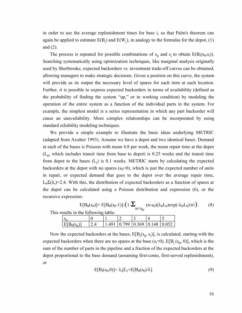
in order to use the average replenishment times for base i, so that Palm's theorem can again be applied to estimate E(Bi) and E(Wi), in analogy to the formulas for the depot, (1) and (2). The process is repeated for possible combinations of s0 and si to obtain E(Bi(s0,si)). Searching systematically using optimization techniques, like marginal analysis originally used by Sherbrooke, expected backorders vs. investment trade-off curves can be obtained, allowing managers to make strategic decisions. Given a position on this curve, the system will provide as its output the necessary level of spares for each item at each location. Further, it is possible to express expected backorders in terms of availability (defined as the probability of finding the system “up,” or in working condition) by modeling the operation of the entire system as a function of the individual parts in the system. For example, the simplest model is a series representation in which any part backorder will cause an unavailability. More complex relationships can be incorporated by using standard reliability modeling techniques. We provide a simple example to illustrate the basic ideas underlying METRIC (adapted from Axsäter 1993). Assume we have a depot and two identical bases. Demand at each of the bases is Poisson with mean 4.8 per week, the mean repair time at the depot (L0, which includes transit time from base to depot) is 0.25 weeks and the transit time from depot to the bases (Li) is 0.1 weeks. METRIC starts by calculating the expected backorders at the depot with no spares (s0=0), which is just the expected number of units in repair, or expected demand that goes to the depot over the average repair time, L0Σ(λi)=2.4. With this, the distribution of expected backorders as a function of spares at the depot can be calculated using a Poisson distribution and expression (6), or the recursive expression:

E[B0(s0)]= E[B0(s0-1)]-(1-ΣΣΣΣn<s0

(n-s0)(λ0L0)exp(-λ0L0)/n!). (8) This results in the following table:

s0 0 1 2 3 4 5 E[B0(s0)] 2.4 1.491 0.799 0.369 0.148 0.052

Now the expected backorders at the bases, E[Bi(s0, si)], is calculated, starting with the expected backorders when there are no spares at the base (si=0), E[Bi (s0, 0)], which is the sum of the number of parts in the pipeline and a fraction of the expected backorders at the depot proportional to the base demand (assuming first-come, first-served replenishment), or

E[Bi(s0,0)]= λi[Li+E[B0(s0)/λ] (9)

17

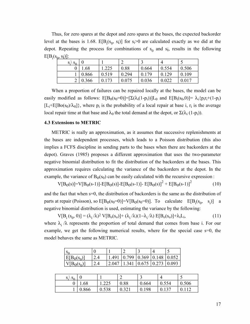
Thus, for zero spares at the depot and zero spares at the bases, the expected backorder level at the bases is 1.68. E[Bi(s0, si)] for si>0 are calculated exactly as we did at the depot. Repeating the process for combinations of s0 and si, results in the following E[Bi(s0, si)]:

si\ s0 0 1 2 3 4 5 0 1.68 1.225 0.88 0.664 0.554 0.506 1 0.866 0.519 0.294 0.179 0.129 0.109 2 0.366 0.173 0.075 0.036 0.022 0.017

When a proportion of failures can be repaired locally at the bases, the model can be easily modified as follows: E[B0(s0=0)]=[Σ(λi(1-pi))]L0 and E[Bi(s0,0)]= λi{piri+(1-pi) [Li+E[Bo(s0)/λ0]}, where pi is the probability of a local repair at base i, ri is the average local repair time at that base and λ0 the total demand at the depot, or Σ(λi (1-pi)).

4.3 Extensions to METRIC

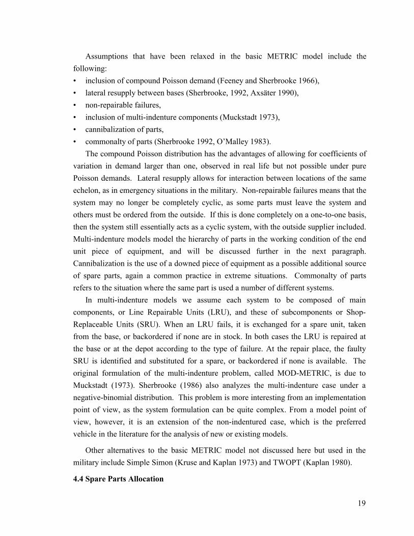
METRIC is really an approximation, as it assumes that successive replenishments at the bases are independent processes, which leads to a Poisson distribution (this also implies a FCFS discipline in sending parts to the bases when there are backorders at the depot). Graves (1985) proposes a different approximation that uses the two-parameter negative binomial distribution to fit the distribution of the backorders at the bases. This approximation requires calculating the variance of the backorders at the depot. In the example, the variance of Bo(s0) can be easily calculated with the recursive expression : V[Bo(s)]=V[Bo(s-1)]-E[Bo(s)]-E[Bo(s-1)]- E[Bo(s)]2 + E[Bo(s-1)]2 (10)

and the fact that when s=0, the distribution of backorders is the same as the distribution of parts at repair (Poisson), so E[Bo(s0=0)]=V[Bo(s0=0)]. To calculate E[Bi(s0, si)] a negative binomial distribution is used, estimating the variance by the following: V[Bi (s0, 0)] = (λi /λ)2 V[Bo(so)]+ (λi /λ)(1−λi /λ) E[Bo(so)]+λiLi, (11) where λi /λ represents the proportion of total demand that comes from base i. For our example, we get the following numerical results, where for the special case s=0, the model behaves the same as METRIC.

s0 0 1 2 3 4 5 E[Bo(s0)] 2.4 1.491 0.799 0.369 0.148 0.052 V[Bo(s0)] 2.4 2.047 1.341 0.675 0.273 0.093

si\ s0 0 1 2 3 4 5

0 1.68 1.225 0.88 0.664 0.554 0.506 1 0.866 0.538 0.321 0.198 0.137 0.112

18

2 0.366 0.196 0.098 0.048 0.027 0.018 Graves (1985) conduced extensive testing and found that METRIC underestimates expected backorders, while his negative binomial approximation overestimates them. The negative binomial approximation gave mistaken allocation of spares in less than 1% of the cases, while METRIC errs in almost 11% of the cases. Note that obtaining the exact distributions is intensive in calculations, as the convolutions must be solve for every value of s0 and the base decomposition done separately for each base. Also, total demand over pipelines must be separately calculated for each base when the pipeline lengths are different, and then convolute into global demand. This is admittedly trivial for Poisson distributions, but still time consuming. The negative binomial approximation seems a better compromise, as it yields good results while being computationally very efficient. Other documented applications of negative binomial distributions, can be found in O’Malley (1983) and Slay (1984) in military applications, and in a retail setting in Svoronos and Zipkin (1991).

For deterministic transit times (times in the pipelines), an exact analysis was also provided by Graves (1985). He finds the distribution of total outstanding orders for all bases by solving the convolution of the backorders distribution at the depot and the total demand over the length of the pipeline from depot to base. More specifically, let Qi(t) be the outstanding orders at epoch t at base i, Q(t) the total amount of outstanding orders at epoch t, and D(t, t+T) the demand in the interval [t, t+T]. Then, for a fixed depot-to-base transportation time T, Q(t+T)=ΣQi(t+T)=B(t|s0)+D(t, t+T), since in the interval [t, t+T], any items in transit from the depot to the bases must have arrived, but any backorders at t could not have arrived yet. Since the demand in interval [t,t+T] is independent of backorders, an exact expression for Q(t+T) can be obtained from the convolution of B(t|s0) and D(t, t+T). If demand is Poisson, then Q (t) is Poisson, since backorders are Poisson. Once this convolution is solved, Q(t) must be decomposed into the Qi(t) components using a binomial distribution (under first-come, first-served base replenishment):

P(Qi(t) =j) = ΣΣΣΣk >j

P(Q(t) =k) k!/((k-j)!j!) (λi /λ)j (λ−λi /λ)k-j. (11) If, as in our simple example, we also include a base-to-depot transportation pipeline, which is necessary if the repair times are not assumed to be independent of the number of parts in repair, then there is an additional superposition that must be considered, and the analysis is more complicated. Approximation methods to handle the case where repair facilities are resource constrained are introduced in Díaz and Fu (1995).

19

Assumptions that have been relaxed in the basic METRIC model include the following: • inclusion of compound Poisson demand (Feeney and Sherbrooke 1966), • lateral resupply between bases (Sherbrooke, 1992, Axsäter 1990), • non-repairable failures, • inclusion of multi-indenture components (Muckstadt 1973), • cannibalization of parts, • commonalty of parts (Sherbrooke 1992, O’Malley 1983). The compound Poisson distribution has the advantages of allowing for coefficients of variation in demand larger than one, observed in real life but not possible under pure Poisson demands. Lateral resupply allows for interaction between locations of the same echelon, as in emergency situations in the military. Non-repairable failures means that the system may no longer be completely cyclic, as some parts must leave the system and others must be ordered from the outside. If this is done completely on a one-to-one basis, then the system still essentially acts as a cyclic system, with the outside supplier included. Multi-indenture models model the hierarchy of parts in the working condition of the end unit piece of equipment, and will be discussed further in the next paragraph. Cannibalization is the use of a downed piece of equipment as a possible additional source of spare parts, again a common practice in extreme situations. Commonalty of parts refers to the situation where the same part is used a number of different systems. In multi-indenture models we assume each system to be composed of main components, or Line Repairable Units (LRU), and these of subcomponents or Shop-Replaceable Units (SRU). When an LRU fails, it is exchanged for a spare unit, taken from the base, or backordered if none are in stock. In both cases the LRU is repaired at the base or at the depot according to the type of failure. At the repair place, the faulty SRU is identified and substituted for a spare, or backordered if none is available. The original formulation of the multi-indenture problem, called MOD-METRIC, is due to Muckstadt (1973). Sherbrooke (1986) also analyzes the multi-indenture case under a negative-binomial distribution. This problem is more interesting from an implementation point of view, as the system formulation can be quite complex. From a model point of view, however, it is an extension of the non-indentured case, which is the preferred vehicle in the literature for the analysis of new or existing models.

Other alternatives to the basic METRIC model not discussed here but used in the military include Simple Simon (Kruse and Kaplan 1973) and TWOPT (Kaplan 1980).

4.4 Spare Parts Allocation

20

Here, we discuss some of the allocation techniques that have been used once a performance characterization technique has been adopted via one of the models already described or some other means such as a simulation model. As the focus of this review is on the models and not on the allocation/optimization schemes, the discussion will be very brief. In METRIC’s original method, allocation was accomplished via the simple procedure of marginal analysis. This approach follows a “more bang per buck” approach, as the spare parts with the greatest marginal contribution of (E[B(s)]-E[B(s-1)) per item cost are progressively added. Sherbrooke showed that the approach was optimal for single echelon cases by proving convexity of the objective function. However, the literature has noted the inefficiencies of the marginal approach in general and has proposed alternatives, such as mathematical programming procedures based on Lagrangean multipliers. Assume we have a budget B that we want use to buy spares of different types. This budget allocation problem can be expressed (Demmy and Presutti 1981) as the minimization of the sum of backorders at all bases for all types, subject to the cost of the required spares (all types at all bases and the depot) not exceeding a given budget B. Fox and Landi (1970) observed that the use of Lagrangean procedures could be more efficient that marginal analysis. If φ is a Lagrange multiplier associated with the budget limitation B, the constraint can be incorporated into the objective function. This can then be separated into single-item optimization problems. For a given level of parts at the depot (s0), Bi(si) is convex with respect to si, so that for a given value of s0 the optimal si can be calculated by obtaining the smallest si that satisfies B(si+1)-B(si)_φci, where Bi(si) is the level of backorders at base i given s spares at that base, and ci is the cost of each part of type i. To find the φ associated with a given B, Fox and Landi suggest a binary search procedure, noting that bounds for its optimal value could be obtained from experience. The program SESAME (Kaplan 1980) implements a version of this approach for the United States Army.

4.5. Queueing Models As is evident by the representation of Figure 5, a multi-echelon system for repairable items can be viewed as a network of queues, as queues are formed at every repair facility and the pipelines can also be represented as queues. Queueing models allow for the relaxation of assumptions in METRIC-based models such as an infinite parts population and an uncapacitated repair facility. However, the fact that the depot and bases are stocking facilities complicates the possibility of modeling using conventional queueing network models. Thus, in the literature, queueing-related analysis falls into two main types:

21

• decomposition into individual queues; • Markov chain representation of the entire system. In the first approach, after the queueing analysis is applied, the key relationships (1)-(4) can then be used to calculate the important measures of performance such as expected backorders. For example, in the simplest version of our model, queueing theory would be used to find the distributions for to determine N1, N2, and N4. In the second approach, the measures of performance are usually calculated directly from the derived probability distribution. A disadvantage of these Markov Chain models, probably inhibiting their propagation, is that even for small problems the state space can be large and solution procedures time consuming. The remainder of this section will first provide an overview of queueing network models — which we feel still have potential unexplored applicability, and then discuss applications of queueing models and more general Markov Chain analyses to repairable item inventory systems.

4.5.1 An Overview of Queueing Network Models Networks of queues, based in the work of Jackson (1963) and Gordon and Newell (1967), can be divided into open, closed and mixed queueing networks; see also Walrand (1988) and Suri et al. (1993). An open network is a system in which every part that enters the system eventually leaves the system, i.e., there are arrival processes to and departure process from the various nodes in the network. In closed networks, on the other hand, the number of parts in the system is fixed. Thus, open networks correspond roughly to acyclic inventory systems, whereas closed networks correspond to cyclic inventory systems. A priori, it would seem, that only closed network models apply to repairable item inventory. However, if the parts population is large enough, it is often advantageous to model the system as an open network, which is what METRIC essentially does (unbeknownst at the time it was introduced), as illustrated in the last section. The most useful types of queueing network models are the product-form networks, so named because the joint probability of queue-lengths at each of the nodes in the system can be expressed as a product of terms based only on each individual node in the network and a normalizing constant, e.g., for a network with two nodes: P(N1=n1,N2=n2)=G(N1,N2)P(N1=n1)P(N2=n2), where G represents the normalizing constant. The classic paper on this is Baskett et al. (1975). For open networks, the normalizing constant is also a product of individual node terms, so the analysis decomposes into individual queueing analyses at each of the nodes. For closed networks, the normalizing constant is dependent on all the nodes simultaneously, which is the source of computational complexity for analyzing these

22

types of networks, even using a simple recursive algorithm for calculating the normalizing constant, the convolution algorithm of Buzen (1973). Thus, if the parts population is large enough, it is often advantageous to model the system as an open network, as the corresponding infinite state space is much easier to analyze (and computationally much more efficient) than a large finite state space. Product-form networks require certain assumptions such as an infinite number of servers at a node or exponential service time distribution, in addition to Poisson arrival processes for open networks. For this reason, an important topic of research has been the development of useful approximations which can be implemented easily. For open networks, the main approach has been a decomposition of the network into individual nodes, which are then analyzed separately, paralleling the product-form results. This requires a characterization of departure processes and arrival processes, along with the superposition and splitting of these processes. Models along this line include the Queueing Network Analyzer of Whitt (1983). For closed queueing networks, a promising technique is Mean Value Analysis (MVA), which is a simple iterative procedure that does not grow combinatorially (and is exact for the product-form special cases); c.f., e.g., Reiser (1981).

4.5.2 Applications to Repairable Item Inventory One of the earliest use of queueing models for repairable item inventory systems is the classic machine repairmen problem found in the queueing chapter of almost every introductory operations research textbook. The key benefits in applying this model is that it allows for finite repair capacity and a population-dependent failure rate; see also Nahmias (1981) for further discussion. More involved queueing models have been proposed by Daryanani and Miller (1992), who use a multiple-source, single server queueing system and backorders evaluation built upon taboo structure of invariant measures; and Jung (1993), who propose a simple analytical solution to a recoverable inventory problem in which the demand is subject to a non stationary failure process. Another paper by Balana et al. (1989) analyzes the problem under non-stationary conditions, arguably interesting in time-varying conditions like war. Gross et al. (1978, 1983) solves a one base model using a closed Jackson network. The optimization is done with an algorithm by Lawler and Bell (1966). Proof of convergence and some application examples are also provided. This method suffer the disadvantage, on top of size restrictions, of being inapplicable in circumstances in which

23

the routing is dependent on the state of the system (e.g., backorders at the bases are filled not on a FCFS basis, but on a priority basis) and of not allowing for spares at the depot.

4.5.3 Applications of More General Markov Chain Models Markov Chain methods are simple enough to apply for very small problems and the repairmen example is commonly used in applied probability textbooks. The first network queueing model in the literature, due to Mirasol (1963), was solved via a birth-and-death model, a Markov Chain with the special structure of allowing only transitions between adjacent states. It is interesting because it precedes METRIC and uses multi-indenture concepts and the idea of unavailability to measure performance. The use of Markov chain modeling can be illustrated with a simple example, similar in structure to the scenario used by Gross et al. in various papers (1987, 1993). At a base, an items is either being locally repaired, in operation, or stocked as a spare part. Operating items fail with failure rates λb (repairable at base) or λd (repairable at depot) and are repaired with rates µb and µd (corresponding to base and depot, respectively), all according to an exponential distribution. Similarly, an item in the depot is either being repaired or available as a spare part. Spares are sent from the depot to the bases only in the event of the arrival of a failed part from the base (but not when the failed part is repaired locally at the base). In the Markov chain representation, the state of the system is represented by a multi-dimensional variable, where for base i, Ri is the number of items being locally repaired, O is the number of items in operation, Si is the number of spare parts available, and for the depot, R0 is the number of parts in repair and S0 is the number of spare parts available. Figure 10(a) gives the schematic representation for a single base and one part, a depot with one spare, and no transportation pipelines (zero transit time between base and depot). Figure 10(b) gives the state transition rate diagram for the Markov chain model, which has five states. For example, a transition from state 1 (one working part at the base and one spare part at the depot ) to state 2 (one working part at the base and one part in repair at the depot ) represents a failure which must be repaired at the depot, in which case the depot sends its spare to the base, the part arriving immediately under the assumption of zero transit times. This problem can be solved via the usual flow balance equations. Although a problem of this size can be solved easily by hand or through the use of specialized software, the number of states grows combinatorially as the formulation becomes more realistic. For one depot, two bases and one part per base the number of states is still a manageable 13, but for one depot, three bases and 40 items per base, the number of states is over 630 million! (see Albright 1989). Two ways of reducing the size of this problem have been

24

explored in the literature, iterative procedures and decomposition methods. The iterative procedures, reviewed in a recent paper by Gross et al. (1993), provide methods for the solution of large linear matrix equations of the general form Ax=b. Specifically, separating A into upper, lower and diagonal matrices, U, L, and D, respectively, we have x=D-1 b-D-1 (L+U)x. This simplifies the inversion but makes the solution implicit, which then requires iteration. Methods for carrying out the iteration include Jacobi iteration, Gauss-Seidel and the bi-conjugate gradient, the last being a decomposition method applied to the transition matrix.

Another approach involves reducing the size of the state space using approximate decomposition techniques. Gross et al. (1987) have proposed a decomposition of the network into overlapping subnetworks. The papers by Albright and Soni (1988), Albright (1989), Gupta and Albright (1992), and Albright and Gupta (1993) also take the decomposition approach. Both Gross and the first Albright models decompose the problem by fixing the number of items owed by the depot to the bases (backorders) and then solving each base as a one-dimensional birth-and-death process (only transitions to and from the local repair facility remain). The depot is also solved via a birth-and-death model, but the problem here is n-dimensional as the state is defined by the vector of items owed to each base (note that no spares are held at the depot in these formulations). The resulting depot matrix is however sparse, so approximations can be used (Gauss-Seidel in both cases). Having obtained both probability matrices, the product will approximate the global probability matrix. Albright improves on this idea by reducing the depot case to a uni-dimensional birth and death (1989) and also by extending the problem to the multi-indenture case (1992). A related paper assumes that different modules are repaired by different servers. Overall, the queueing models discussed suffer the disadvantage of additional complexity, of being limited to first-come, first-served service to the bases, and of assuming Poisson failure and repair processes. Another important disadvantage of these methods is that they almost all assume a single class problem (e.g., the servers are dedicated to repair one type of failure only and are not shared among different items or failure modes), although a multi-class problem has was recently considered in Gupta and Albright (1993). General Markov chain modeling does allow for more realistic modeling (other than the Poisson assumptions, which must be retained), but suffers from combinatorial state space explosion. In conclusion, to our knowledge, implementation of these queueing methods for spare parts management in industrial practice is rare, in contrast to the widespread use of METRIC-based models in the military world.

25

5. Directions for Further Research

In this section, we discuss the following key components in multi-echelon repairable item models which we believe must be addressed in order to make the models applicable to industrial application of spare parts management, as opposed to their present prevalent use in military settings:

• repair classes and parts dispatching policies;

• resource constrained repair facilities and size of parts population;

• batching.

We then conclude the review by briefly mentioning the use of simulation, which we have a feeling is the most commonly used method in industry at present.

5.1. Repair classes and dispatching policies

In a multiclass environment, characterized by different classes of items sharing common repair and transportation facilities, complexities arise in determining priorities/policies for

(i) repairing parts that arrive at the repair facilities and must queue, and

(ii) dispatching repaired parts when multiple bases have outstanding backorders.

The decision on the first item, which parts to repair next, is avoided in the METRIC-like models, where the repair facilities are assumed unconstrained (infinite), but this is unlikely to be realistic in industrial practice. The most likely scenarios would be either first-come, first-served (FCFS) or a priority-based scene, either fixed (as in certain parts always have a higher priority) and/or dynamic (as in one base is in an “emergency” situation). Most of the queueing models for the repair facility in the literature assume FCFS, so more work to apply models based on priorities (which do exist in the queueing literature for other applications) is needed.

The second item involves priorities on depot dispatching among competing demands from the bases, especially in a backordered situation. Possible policies include FCFS, fixed proportional routing, priority dispatching, and state-dependent dispatching. Up until now, all the analytical models, with the exception of the Markov chain models, have assumed FCFS dispatching for parts from the depot. Under FCFS, parts from the depot are pulled into the bases as demand occurs. If there is a backorder situation at the depot, parts are sent to the bases, as repairs are concluded, in the order in which they were demanded. This is an underlying assumption of METRIC. Other non-METRIC models

26

that utilize this discipline are the Markovian models of Albright (19989, 1993). An argument given in the literature to support this assumption is that it is easier to control, as the depot doesn’t have to know the state of the bases at all times. Another common argument is that this method is ‘fair’ (Axsäter 1993). Under fixed proportional routing, parts are sent to the bases on a fixed ratio basis, i.e., a fixed proportion of the parts, pi, is sent to base i. This assumption allows to model the system using closed queueing network methods, although it does not adjust dynamically to the changing conditions of the system (e.g., if a base start having an “epidemic”, or burst of failures, more parts should go to that base). This discipline is implicit in queueing network models such as Gross (1983), or in methods such as Mean Value Analysis (Reiser 1981) for closed queueing networks and decomposition approaches for open queueing networks (Whitt 1983). Under state-dependent dispatching priorities, parts will be sent according to centralized information on backorders at the bases. For example, the depot might choose to send a repaired part to the base with the worst availability (or backorder) situation. Otherwise this policy is similar to a FCFS and we should expect both disciplines to show similar results when the expected backorders at the depot is small. As mentioned already, Markov chain models can support these disciplines (i.e., see Gross 1987, 1992), but usually at the cost of intractability for systems of practical size. This can also be combined with some fixed priority scheme, such as those examined by Dada (1992), Cohen et al. (1992) and Pyke (1990), where return priorities are assigned to different classes, either on a predetermined or ad-hoc basis. Critical parts are expedited through the system with a shorter pipeline, at a higher cost. If some classes of parts are to be expedited when distributed, it seems logical that they should also be expedited in the repair process. As there are few analytical results for this type of multiclass problem, Pyke (1990) has used simulation to analyze the effect of priorities on both repair and distribution policies, and he states that “the distribution rule at the depot has little effect for all but a small subset of parameters” and that repair priority disciplines only have a significant effect in cases of high utilization of the repair facility (ρ>0.9) and in these cases, the effect is lost unless a priority discipline is also used for the distribution process. However, we feel that there is more that can be done here.

5.2. Constrained Repair Facilities and Finite Parts Population We mentioned how most documented implementations of multi-echelon models for repairable items are METRIC-like military applications. While two important assumptions of METRIC, infinite calling population and repair capacity can be acceptable

27

in military environments, they seem more restrictive in industrial applications, where both the calling population and the repair capacity are likely to be limited. It is interesting to note that apart from the Muckstadt and Gross investigations mentioned earlier, little research has been conducted on studying how restrictive these constraints are for industrial applications. Queueing approaches, originally developed to overcome these shortcomings, at present generally result in complex models of limited practical appeal. Some work along this line can be found in Díaz (1995) and Díaz and Fu (1995), where simple approximations based on Whitt (1993) are employed. For high repair facility utilization, the improvement over METRIC-like models is very significant.

5.3. Batching In industry, it is likely that batching of parts sent between bases and depot would be likely, so that the operating policies would involve two parameters at each stocking location. Models to handle batching are thus critical. Axsäter (1993) notes that analytical results are available only for a few special cases which are not likely to be representative of situations found in industry: only a single base, or batching only at the depot. In addition, Poisson failure processes must be assumed. Cohen et al. (1992) is one attempt to tackle the more general problem, but this topic is definitely a fertile area for further research.

5.4. Simulation Finally, we conclude by noting that both Nahmias (1981) and Gross (1993) call for the use of hybrid models that involve simulation. Discrete event stochastic simulation is commonly used for benchmarking purposes and is in principle a perfectly flexible tool in that almost any real life conditions can be modeled. Its use for multi-echelon inventory models dates at least as far back as Clark (1960). Its main drawback is its computational expense, and it is rarely used to do any sort of real optimization beyond naive trial and error of a few policies. In practice, we believe that most spare parts management is done by a series of ad hoc “seat-of-the-pants” approaches. For example, in a case study discussed in Fu and Díaz (1995), the industry user simply follows the supplier's recommendations for spare parts target levels which are based on “experience” of the supplier. At best, once the target levels are set, simulation is then used to do performance analysis of the system, but not optimization, per se. There are of course exceptions, such as the one documented by Bier and Tjelle (1994), who describe spares inventory planning in the Boeing aircraft company, employing experimental design techniques in conjunction with their simulation model. Our feeling echoes that of Nahmias (1981) and Gross (1993), specifically by suggesting that sequential improvement algorithms such as

28

Response Surface Methodology (RSM) and gradient-based procedures based on stochastic approximation can be employed fruitfully (see, e.g., Fu 1994 for an overview of techniques for optimization via simulation) in conjunction with analytical techniques, for example by finding an initial feasible solution with approximate methods (like METRIC) in order to reduce the size of the search space. Moreover, advances in the use of parallel computing will help to make this approach more computationally feasible.

29

References Albright, S. “An approximation to the stationary distribution of a Multiechelon

repairable-item inventory system with finite sources and repair channels.” Naval Research Logistics v36 179-195 1989.

Albright, S., Gupta, A. “Steady-State Approximation of a Multiechelon Multi-Indentured repairable-Item Inventory System with a Single Repair Facility.” Naval Research Logistics v40 n4 479-493 Jun. 1993.

Albright, S., Soni, A. “Markovian Multiechelon Repairable Inventory System.” Naval Research Logistics v35 49-61 1988.

Allen, S., d'Esopo, D.; “An ordering policy for repairable stock items.” Operations Research v16 n3 669-674 1968.

Arrow, K., Karlin, S. and Scarf, H. Mathematical Theory of Inventory and Production, Stanford University Press, Stanford, 1958.

Arrow, K., Karlin, S. and Scarf, H. Studies in Applied Probability and Management Science, Stanford University Press, Stanford, 1962.

Axsäter, S. “Continuous Review Policies for Multi-Level Inventory Systems with Stochastic Demand.” In S. Graves, A. Rinnooy Kan and P. Zipkin (Ed.) Logistics of Production and Inventory, North Holland, Amsterdam 1993.

Axsäter, S. “Modeling emergency lateral transshipments in inventory systems.” Management Science v36 n11 1329-1338 Nov. 1990.

Balana, A., Gross D., Soland, R. “Optimal Provisioning for Single-Echelon Repairable Item Inventory Control in a Time-Varying Environment.” IIE Transactions v21 n3 202-212 1989.

Baskett, F., Chandy, K., Muntz, R., Palacios, F., “Open, Closed and Mixed Networks of Queues with Different Classes of Customers,” Journal of the Association for Computer Machinery v22 n2 248-260 Apr. 1975.

Bier, I.J. and Tjelle, J.P.. “The Importance of Interoperability in a Simulation Prototype for Spares Inventory Planning.” Proceedings of the 1994 Winter Simulation Conference, pp. 913-919.

Buzen, J. “Computational Algorithms for Closed Queueing Networks with Exponential Servers.” Communications of the ACM, v16 p527 1973.

Clark, A. “An informal survey of multi-echelon inventory theory.” Naval Research Logistics Quarterly v19 p621 1972.

Clark, A. “Experiences with a Multi-indenture, Multi-echelon inventory model.” In Schwarz (Ed.) Multi-level Production/Inventory Control Systems: Theory and Practice, v16, Studies in the Management Science, North Holland, Amsterdam 1981.

Clark, A. “The use of simulation to evaluate a multi-echelon, dynamic inventory model.” Naval Research Logistics v7 429-445 1960.

30

Clark, A. and Scarf, H., “Optimal Policies for Multi-Echelon Inventory Problem.” Management Science v6 p475 1960.

Clark, A. and Scarf, H. “Approximate solutions to a Simple Multi-Echelon Inventory Problem.” In Arrow, K., Karlin, S. and Scarf, H. (Ed.) Studies in Applied Probability and Management Science, Stanford University Press, Stanford, 1962.

Cohen, M., Kamesam, P., Kleindorfer, P., Lee, H. Tekerian, A. “Optimizer: IBM's multi-echelon inventory system for managing service logistics.” Interfaces v20 n1 65-82 1990.

Cohen, M., Kleindorfer, P., Lee, H, Pyke, D. “Multi-item service constrained (s, S) policies for spare parts logistics.” Naval Research Logistics v39 n4 561-577 1992.

Dada, M. “A Two-Echelon Inventory System with Priority Shipments.” Management science v38 n8 1140-1153 1992.

Daryanani, S., Miller, D. “Calculation of steady-state probabilities for repair facilities with multiple sources and dynamic return priorities.” Operations Research v40 s2 248-256 1992.

Demmy, W., Presutti, V. Multi-echelon inventory theory in the air force logistics command.” In Schwarz (Ed.) Multi-level Production/Inventory Control Systems: Theory and Practice, v16, Studies in the Management Science, North Holland, Amsterdam 1981.

Díaz, A. and Fu, M. C. “Models for Multi-Echelon Repairable Item Inventory Systems with Limited Repair Capacity” submitted to European Journal of Operational Research. 1995.

Díaz, A., Multi-Echelon Models for Repairable Items, Ph.D. dissertation, University of Maryland, College Park, College of Business and Management, 1995.

Federgruen, A., “Centralized Planning models,” in Logistics of Production and Inventory, editors S. Graves, A. Rinnooy Kan and P. Zipkin, North Holland, 1993.

Feeney G., Sherbrooke, C. “The (s-1, s) Inventory Policy under Compound Poisson Demand.” Management Science v12 p391 1966.

Fox, B. and Landi, D. “Searching for the multiplier in one constraint optimization problems.” Operations Research v18 n2 253-262 1970.

Fu, M. “Optimization via Simulation: A Review.” Annals of Operations Research v53 199-246 1994.

Gordon, W. and Newell, G. “Closed Queueing Systems with Exponential Servers.” Operations Research v15 n2 254-265 1967.

Graves, S. “A multi-echelon inventory model for a repairable item with one-for-one replenishment.” Management Science v31 n10 1247-1256 1985.

Graves, S., Rinnooy Kan, A. and Zipkin, P. (Ed.) Logistics of Production and Inventory, North Holland, Amsterdam 1993.

31

Gross, D, Gu, B., Soland R. “Iterative solution methods for obtaining steady state probability distributions of Markovian Multi-echelon repairable items inventory systems.” Computer & Operations Research v20 n8 817-828 1993.

Gross, D. and Ince, J. “A closed queueing Network Model for Multi-Echelon Repairable Items Provisioning.” IIE Transactions v10 307 1978.

Gross, D., Kioussin L., Miller, D. “A Network decomposition approach for approximate steady state behavior of Markovian Multi-Echelon Repairable item inventory systems.” Management Science v33 1453-1468 1987.

Gross, D., Miller, D., Soland, R. “A closed queueing Network Model for Multi-Echelon Repairable Item Provisioning”. IIE Transactions v15 n4 344-352 1983.

Gupta, A., Albright, S. “Steady-state approximations for a multi-echelon multi-indentured repairable-item inventory system.” European Journal of Operational Research v62 n3 p340 Nov. 1992.

Hadley, G. and Whitin, T. Analysis of Inventory Systems, Prentice Hall, Englewood Cliffs, New Jersey, 1963.

Hayes and Wheelright. “Link manufacturing Process and Product Life Cycles.” Harvard Business Review v57 p133 Jan.-Feb. 1979.

Jackson, J. “Jobshop-Like Queueing Systems.” Management Science v10 p131 1963.

Jung, W. “Recoverable Inventory Systems with Time-Varying Demand.” Production and Inventory Management Journal v34 n1 77-81 1993.

Kaplan, A. “Mathematics for SESAME Model.” Technical report no. TR80-2 US. Army Inventory Research Office, Philadelphia PA 1980.

Kruse, W., Kaplan, A. “On a paper by Simon.” Operations Research v21 n6 1318-1321 1973.

Lawler, E. and Bell, M. “A Method of Solving Discrete Optimization Problems.” Operations Research v14 n6 1098-1112 1966.

Mirasol, N. “A Queueing Approach to Logistics Systems.” Operations Research v12 707-724 1963.

Muckstadt, J and Thomas, L. “Are multi-echelon inventory models worth implementing in systems with low-demand rates?” Management Science v26 483-494 1980.

Muckstadt, J. “A model for multi-item, multi-echelon, multi-indenture inventory system.” Management Science v20 p472 1973.

Muckstadt, J. and Roundy, R., “Analysis of Multistage Production Systems.” In S. Graves, A. Rinnooy Kan and P. Zipkin (Ed.) Logistics of Production and Inventory, North Holland, Amsterdam 1993.

Nahmias, S. “Managing Reparable item inventory systems: A review.” In Schwarz (Ed.) Multi-level Production/Inventory Control Systems: Theory and Practice, v16, Studies in the Management Science, North Holland, Amsterdam 1981.

32

O’Malley, personal communication, 1994.

O’Malley, T. The Aircraft Availability Model: Conceptual Framework and Mathematics, Logistics Management Institute, 1983.

Pyke, D. “Priority Repair and Dispatch Policies for Reparable-Item Logistics Systems.” Naval Research Logistics v37 n1 1-30 Feb. 1990.

Reiser, M. “Mean-Value Analysis and Convolution Method for Queue-Dependent Servers in Closed Queueing Networks.” Performance Evaluation v1 n1 7-18 1981.

Scarf, H., Gilford, D. and Shelley, M. Multistage Inventory Models and Techniques, Stanford University Press, Stanford, 1963.

Schmenner, R. Production/Operations Management. Concepts and Situations. SRA, 1981.

Schmenner, R. “How can service business survive and prosper?” Sloan Management Review, 21-32 Spring 1986.

Schwarz, L., Multi-level Production/Inventory Control Systems: Theory and Practice, North Holland, Amsterdam, 1981.

Sherbrooke, C. “METRIC: A multi-echelon technique for recoverable item control.” Operations Research v16 n2 122-141 1968.

Sherbrooke, C. "VARI-METRIC: Improved approximation for multi-indenture, multi-echelon availability models.” Operations Research v34 n2 311-319 1986.

Sherbrooke, C. Optimal Inventory Modeling of Systems, Wiley and Sons, New York, 1992.

Sherbrooke, C. “Multiechelon Inventory Systems with Lateral Supply.” Naval Research Logistics v39 n1 29-40 Feb. 1992.

Simon, R. “Stationary properties of a two-echelon inventory model for low demand items” Operations Research v19 n3 761-773 1971.

Slay, F. “VARI-METRIC” Logistics Management Institute 1984.

Suri, R., Sanders, J. and Kamath, M. “Performance Evaluation of Production Networks.” In S. Graves, A. Rinnooy Kan and P. Zipkin (Ed.) Logistics of Production and Inventory, North Holland, Amsterdam 1993.

Svoronos, A. and Zipkin, P. “Evaluation of one-for-one replenishment policies for multiechelon inventory systems.” Management Science v37 n1 68-83 Jan. 1991.

Walrand, J. An Introduction to Queueing Networks, Prentice Hall, Englewood Cliffs, New Jersey, 1988.

Whitt, W., “The Queueing Network Analyzer.” The Bell Systems Technical Journal v66 n9 2779-2815 Nov. 1983.

Whitt, W., “Approximations for the GI/G/m Queue.” Production and Operations Management v2 n2 114-161 Spring 1993.

Figure 1. The Repair Cycle

m working parts + si spares

Transit

Spares: s0

Bases

Depot

0

iim

Process

Project Construction Jobbing Job-shop Batch Apparel Line Cars

Continuous Petrochemical

volume

Product

Figure 2. Product-Process Matrix

Customizing level: Low High

High

Intensity of

Service factories

Airlines, Common Motor

carriers, Subways

Service stores

Hospitals, Health Maintenance

Organizations

equipment use

Low

Massive services

Department stores, fast food

restaurants

Personal services

Lawyers, Accountants

Figure 3. Services Matrix

High variety of consumables, repairables

critical for continuity of operations

Less variety of consumables,

repairables are very critical

Consumables for support,

repairables not important

Consumables very important,

repairables are less important

va r i e t y

Multi-Echelon

AcyclicInventory

CyclicInventory Re-order point

replenishment

One-for-onereplenishment

Batchedreplenishment

SingleEchelon

Time-varyingdependent demand Lot-sizing algorithms

Independent stationarydemand

Fixed lot size

Fixed interval

Dependent time-varyingdemand

Independent stationary demand

Fixed period replenishment

METRICGravesQueueingNetwork models

Figure 4. Taxonomy of Inventory Models

Depot

( )

1Base

i

s =1s =10

Figure 5. Schematic Representation of the System

Base In-pipeline Repair Stock atDepot

Out-pipeline Stock atthe base

Repair +in-pipeline

1st. convolution: 2d. convolution: Outstandingparts atthe bases

s1 2

34

0 si 5NN

NNN

Figure 6. Relationship Between System Processes

1 2 3 4 5 61 2 3 4 5 6

Base

Repair Pipeline

Depot N (t)1

N (t)

N (t)

N (t)

3

4

t

t

t2

s si 0

Figure 7. Trajectories of parts

s1 DepotRepair

Figure 8. Backorder distribution at the depot

si

s0 Depot

Pipeline+

Base

(inverted)

Figure 9. Outstanding order distribution at the bases

N5(t)

superposition: 2nd. superposition:

s

N3(t)

N4(t)N2(t)

i

In-pipeline (1) Repair (2) Depot (3) Out-pipeline (4) Base (5)

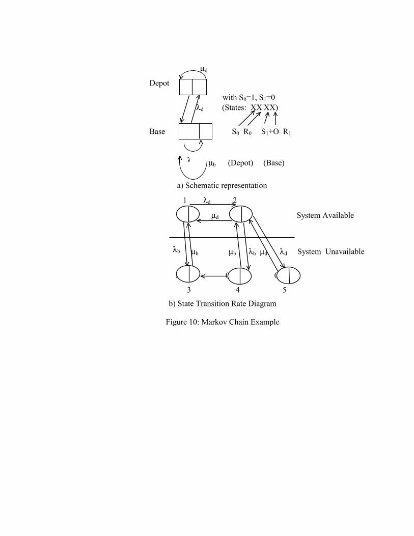
µd

Depot S0 R0

with S0=1, S1=0 λd (States: XX|XX)

Base S1+O R1 S0 R0 S1+O R1

λ b µb (Depot) (Base)

a) Schematic representation

1 λd 2

10 10 µd 01 10 System Available

λb µb µb λb µd λd System Unavailable

10 01 01 01 02 00

3 4 5

b) State Transition Rate Diagram

Figure 10: Markov Chain Example