multi-dimensional index structures part i: motivation
TRANSCRIPT

Multi-dimensional index structuresPart I: motivation
144

Motivation: Data Warehouse
A definition
“A data warehouse is a repository of in-tegrated enterprise data. A data ware-house is used specifically for decisionsupport, i.e., there is (typically, or ide-ally) only one data warehouse in an en-terprise. A data warehouse typically con-tains data collected from a large numberof sources within, and sometimes alsooutside, the enterprise.”
145

Decision support (1/2)
‘Traditional” relational databases were designed for online transactionprocessing (OLTP):
• flight reservations; bank terminal; student administration; . . .
OLTP characteristics:
• Operational setting (e.g., ticket sales)
• Up-to-date = critical (e.g., do not book the same seat twice)
• Simple data (e.g., [reservation, date, name])
• Simple queries that only access a small part of the database (e.g., “Give the flightdetails of X” or “List flights to Y”)
Decision support systems have different requirements.
146

Decision support (2/2)
Decision support systems have different requirements:
• Offline setting (e.g., evaluate flight sales)
• Historical data (e.g., flights of last year)
• Summarized data (e.g., # passengers per carrier for destination X)
• Integrates different databases (e.g., passengers, fuel costs, maintenance informa-tion)
• Complex statistical queries (e.g., average percentage of seats sold per month anddestination)
147

Decision support (2/2)
Decision support systems have different requirements:
• Offline setting (e.g., evaluate flight sales)
• Historical data (e.g., flights of last year)
• Summarized data (e.g., # passengers per carrier for destination X)
• Integrates different databases (e.g., passengers, fuel costs, maintenance informa-tion)
• Complex statistical queries (e.g., average percentage of seats sold per month anddestination)
Taking these criteria into mind, data warehouses are tuned for onlineanalytical processing (OLAP)
• Online = answers are immediately available, without delay.
148

The Data Cube: Generalizing Cross-Tabulations
Cross-tabulations are highly useful for analysis
• Example: sales June to August 2010
Blue Red Orange Total
June 51 25 128 234
July 58 20 120 198
August 65 22 51 138
Total 174 67 329 570
149

The Data Cube: Generalizing Cross-Tabulations
Cross-tabulations are highly useful for analysis
Data Cubes are extensions of cross-tabs to multiple dimensions
Blue Red Orange Total
June 51 25 128 234
July 58 20 120 198
August 65 22 51 138
Total 174 67 329 570
Aggregated w.r.t. Dimension Y
Aggregated w.r.t Dimension X
Aggregated w.r.t Dimension X and Y
Dimension X
Aggregated w.r.t Dimension X
Dim
en
sio
n Y
150

The Data Cube: Generalizing Cross-Tabulations
Cross-tabulations are highly useful for analysis
Data Cubes are extensions of cross-tabs to multiple dimensions
151

OLAP Operations on the CUBE
Roll-up
• Group per semester instead of per quarter
152

OLAP Operations on the CUBE
Roll-up
• Show me totals per semester instead of per quarter
153

OLAP Operations on the CUBE
Roll-up
• Show me totals per semester instead of per quarter
Inverse is drill-down
154

OLAP Operations on the CUBE
Slice and dice
• Select part of the cube by restricting one or more dimensions
• E.g, restrict analysis to Ireland and VCR
155

OLAP Operations on the CUBE
Slice and dice
• Select part of the cube by restricting one or more dimensions
• E.g, restrict analysis to Ireland and VCR
156

Different OLAP systems
Multidimensional OLAP (MOLAP)
• Early implementations used a multidimensional array to store the cube completely:• In particular: pre-compute and materialize all aggregations
157
Array: cell[product, date, country]
• Fast lookup: to access cell[p,d,c] justuse array indexation

Different OLAP systems
Multidimensional OLAP (MOLAP)
• Early implementations used a multidimensional array to store the cube completely:• In particular: pre-compute and materialize all aggregations
158
Array: cell[product, date, country]
• Fast lookup: to access cell[p,d,c] justuse array indexation
• Very quickly people realized that thisis infeasible due to the data explosionproblem
The data explosion problem
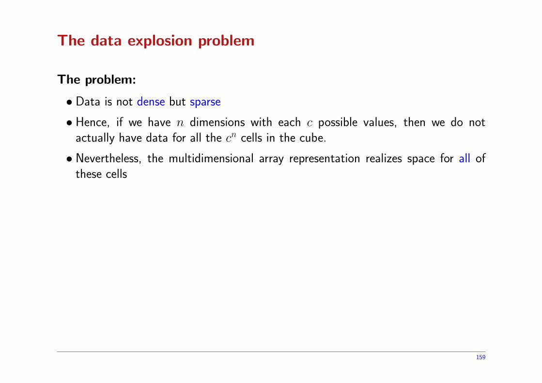
The problem:
• Data is not dense but sparse
• Hence, if we have n dimensions with each c possible values, then we do notactually have data for all the cn cells in the cube.
• Nevertheless, the multidimensional array representation realizes space for all ofthese cells
159

The data explosion problem
The problem:
• Data is not dense but sparse
• Hence, if we have n dimensions with each c possible values, then we do notactually have data for all the cn cells in the cube.
• Nevertheless, the multidimensional array representation realizes space for all ofthese cells
Example: 10 dimensions with 10 possible values each
• 10 000 000 000 cells in the cube
• suppose each cell is a 64-bit integer
• then the multidimensional-array representing the cube requires ≈ 74.5 gigabytesto store → does not fit in memory!
• yet if only 1 000 000 cells are present in the data, we actually only need to store≈ 0.0074 gigabytes
160

Multidimensional OLAP (MOLAP)
In conclusion
• Naively storing the entire cube does not work.
• Alternative representation strategies use sparse main memory index structures:
◦ search trees
◦ hash tables
◦ . . .• And these can be specialized to also work in secondary memory→ multidimensional indexes (the main technical content of this lecture).
161

Relational OLAP (ROLAP)
Key Insight [Gray et al, Data Mining and Knowledge Discovery, 1997]
• The n-dimensional cube can be represented as a traditional relation with n + 1columns (1 column for each dimension, 1 column for the aggregate)
• Use special symbol ALL to represent grouping
162
Product Date Country Sales
TV Q1 Ireland 100
TV Q2 Ireland 80
TV Q3 Ireland 35
... ... ... ...
PC Q1 Ireland 100
... ... ... ...
TV ALL Ireland 215
TV ALL ALL 1459
... ... ... ...
ALL ALL ALL 109290

Relational OLAP (ROLAP)
Key benefits: space usage
• The non-aggregate cells that are not present in the original data are also notpresent in the relational cube representation.
•Moreover, it is straightforward to represent only aggregation tuples in which alldimension columns have values that already occur in the data
163
Product Date Country Sales
TV Q1 Ireland 100
TV Q2 Ireland 80
TV Q3 Ireland 35
... ... ... ...
PC Q1 Ireland 100
... ... ... ...
TV ALL Ireland 215
TV ALL ALL 1459
... ... ... ...
ALL ALL ALL 109290

Relational OLAP (ROLAP)
Key benefits
• By representing the cube as a relation it can be stored in a “traditional” relationalDBMS ...
• ... which works in secondary memory by design (good for multi-terraby datawarehouses) ...
• Hence one can re-use the rich literature on relational query storage and queryevaluation techniques,
But, to be honest, much research was done to get this representationefficient in practice.
164

Relational OLAP (ROLAP)
Key benefits: use SQL
• Dice example: restrict analysis to Ireland and VCR
165
SELECT Date, Sales
FROM Cube_table
WHERE Product = "VCR"
AND Country = "Ireland"
Date Sales
Q1 100
Q2 80
Q3 35
ALL 215

Relational OLAP (ROLAP)
Key benefits: use SQL
• Dice example: restrict analysis to Ireland and VCR, quarter 2 and quarter 3→ need to compute a new total aggregate for this sub-cube
166
(SELECT Date, Sales
FROM Cube_table
WHERE Product = "VCR"
AND Country = "Ireland"
AND (Date = "Q2" OR Date = "Q3")
AND SALES <> "ALL")
UNION
(SELECT "ALL" as DATE, SUM(T.Sales) as SALES
FROM Cube_table t
WHERE Product = "VCR"
AND Country = "Ireland"
AND (Date = "Q2" OR Date = "Q3")
AND SALES <> "ALL"
GROUP BY Product, Country)
This actually motivated the extension of SQL with CUBE-specific operators and keywords

Three-tier architecture
167

Multi-dimensional index structuresPart II: index structures
168

Multidimensional Indexes
Typical example of an application requiring multidimensional searchkeys:
Searching in the data cube and searching in a spatial database
Typical queries with multidimensional search keys:
• Point queries:◦ retrieve the Sales total for the product TV sold in Ireland, with an ALL valuefor date.
◦ does there exist a star on coordinate (10, 3, 5)?
• Partial match queries: return the coordinates of all stars with x = 5 and z = 3.
• Dicing / Range queries:
◦ return all cube cells with date ≥ Q1 and date ≤ Q3 and sales ≤ 100;
◦ return the coordinates of all stars with x >= 10 and 20 ≤ y ≤ 35.
• Nearest-neighbour queries: return the three stars closest to the star at coordinate(10, 15, 20).
169

Multidimensional Indexes
Indexes for search keys comprising multiple attributes?
• BTree: assumes that the search keys can be ordered. What order can we put onmultidimensional search keys?
→ Pick the lexicographical order:
(x, y, z) ≤ (x�, y�, z�) ⇔ x < x�
∨(x = x� ∧ y < y�)∨(x = x� ∧ y = y� ∧ z ≤ z�)
• Hash table: assumes a hash function h : keys → N. What hash function can weput on multidimensional search keys?
→ Extend the hash function to tuples:
h(x, y, z) = h(x) + h(y) + h(z)
170

Multidimensional Indexes
Problem with the lexicographical order in BTrees:
Assume that we have a BTree index on (age, sal) pairs.
• age < 20: ok
• sal < 30: linear scan
• age < 20 ∧ sal < 20
age
sal
9 10 11
10
20
30
40
50
60
70
171

Multidimensional Indexes
Problem with hash tables:
Assume that we have a hash table on (age, sal) pairs.
• age < 20: linear scan
• sal < 30: linear scan
• age < 20 ∧ sal < 20: linear scan
Conclusion: for queries with multidimensional search keys we want toindex points by spatial proximity
.
172

Multidimensional Indexes
Grid files: a variant on hashing
40 55 1000
90
255
500
173

Multidimensional Indexes
Grid files: a variant on hashing
40 55 1000
90
255
500
174

Multidimensional Indexes
Grid files: a variant on hashing
40 55 1000
90
255
500
Bucket
Bucket
Bucket
Bucket
Bucket
BucketBucket
Bucket
Bucket
• Insert: find the corresponding bucket,and insert.
If the block is full: create overflowblocks or split by creating new sepa-rator lines (difficult).
• Delete: find the corresponding bucket,and delete.
Reorganize if desired
175

Multidimensional Indexes
Grid files: a variant on hashing
40 55 1000
90
255
500
Bucket
Bucket
Bucket
Bucket
Bucket
BucketBucket
Bucket
Bucket
• Good support for point queries
• Good support for partial match queries
• Good support for range queries
→ Lots of buckets to inspect, but alsolots of answers
• Reasonable support for nearest-neighbour queries
→ By means of neighbourhoodsearching
• But: many empty buckets when thedata is not uniformly distributed
176

Multidimensional Indexes
Partitioned Hash Functions
Assume that we have 1024 buckets available to build a hashing index for (x, y, z).We can hence represent each bucket number using 10 bits. Then we can determinethe hash value for (x, y, z) as follows:
0 10
f(x) g(y) h(z)
2 7
• Good support for point queries
• Good support for partial match queries
• No support for range queries
• No support for nearest-neighbour queries
• Less wasted space than grid files
177

Multidimensional Indexes
kd-Trees
40 55 1000
90
255
500
178

Multidimensional Indexes
kd-Trees
40 55 1000
90
255
500
179

Multidimensional Indexes
kd-Trees
40 55 1000
90
255
500
180

Multidimensional Indexes
kd-Trees
40 55 1000
90
255
500
181

Multidimensional Indexes
kd-Trees
40 55 1000
90
255
500
182
Multidimensional Indexes
kd-Trees
40 55 1000
90
255
500
183

Multidimensional Indexes
kd-Trees
40 55 1000
90
255
500
184

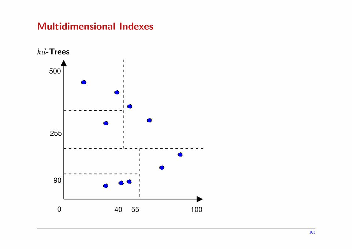
Multidimensional Indexes
kd-Trees
We can look at this as a tree as follows:
X 40
Y 90
X 55
Y 200
X 48
Y 300
40 55 1000
90
255
500
185

Multidimensional Indexes
kd-Trees
We continue splitting after new insertions:
X 40
Y 90
X 55
Y 200
X 48
Y 300
40 55 1000
90
255
500
Y 30
186

Multidimensional Indexes
kd-Trees
• Good support for point queries
• Good support for partial match queries: e.g., (y = 40)
• Good support for range queries (40 ≤ x ≤ 45 ∧ y < 80)
• Reasonable support for nearest neighbour
X 40
Y 90
X 55
Y 200
X 48
Y 300
40 55 1000
90
255
500
187

Multidimensional Indexes
kd-Trees for secondary storage
• Generalization to n children for each interal node (cf. BTree).
But it is difficult to keep this tree balanced since we cannot merge the children
•We limit ourselves to two children per node (as before), but store multiple nodesin a single block.
188

Multidimensional Indexes
R-Trees: generalization of BTrees
Designed to index regions (where a single point is also viewed as a region). Assumethat the following regions fit on a single block:
road1
road
2 pipelinehouse1
house2
school
house1 20,20 30,25road1 0, 40 50,45road2 45, 0 50,40school 20,70 30,75house2 60,40 80,60pipeline 30,21 100,24
100
0 100
189

Multidimensional Indexes
R-Trees: generalization of BTrees
A new region is inserted and we need to split the block into two. We create atree structure:
road1
road
2 pipelinehouse1
house2
theaterschool
house1 20,20 30,25
road1 0, 40 50,45
road2 45, 0 50,40
school 20,70 30,75house2 60,40 80,60pipeline 30,21 100,24
60,70 80,75theatre
100
0 100
(0,0),(55,55) (15,24),(100,80)
190
Multidimensional Indexes
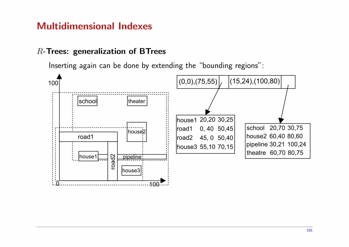
R-Trees: generalization of BTrees
Inserting again can be done by extending the “bounding regions”:
house3
road1
road
2 pipelinehouse1
house2
theaterschool
house1 20,20 30,25
road1 0, 40 50,45
road2 45, 0 50,40
house3 55,10 70,15
school 20,70 30,75house2 60,40 80,60pipeline 30,21 100,24
60,70 80,75theatre
100
0 100
(0,0),(75,55) (15,24),(100,80)
191

Multidimensional Indexes
R-Trees: generalization of BTrees
• Ideal for “where-am-I” queries
• Ideal for finding intersecting regions
e.g., when a user highlights an area of interest on a map
• Reasonable support for point queries• Good support for partial match queries: e.g., (40 ≤ x ≤ 45)
• Good support for range queries
• Reasonable support for nearest neighbour• Is balanced• Often used in practice
192