multi-agent learning no-regret learning - utrecht university · multi-agent learning no-regret...

Multi-agent learning No-regret Learning

Multi-agent learningNo-regret Learning

Gerard Vreeswijk, Intelligent Systems Group, Computer Science Department,

Faculty of Sciences, Utrecht University, The Netherlands.

Gerard Vreeswijk. Last modified on February 16th, 2012 at 10:52 Slide 1


No-regret learning: motivation

• Reinforcement

Learning. Play those

actions that were

successful in the past.

• No-regret learning: might be considered as

an extension of reinforcement learning

No-regret =Def play those actions that

would have been successful in the past.

– Similarities:

1. Driven by pastpayo�s.2. Not interested in

(the behaviour

of) the opponent.

3. Probabilistic.

4. Smooth

adaptation.

5. Myopic.

– Differences:

a) Keeping accounts of hypothetical actions

rests on the assumption that a player is

able to estimate payoffs of actions that

were actually not played.

[Knowledge of the payoff matrix

certainly helps, but is an even more

severe assumption.]

b) Bit more easy to obtain results regarding

performance.



Qualitative features of reinforcement and regret

1. Probabilistic choice. A choice of action is never completely determined

by history but has a random component.

• The different magnitudes of the probabilities (arisen through

experience) ensures exploitation of past experience.

• The randomness ensures exploration.

2. Smooth adaptation. The mixed strategy adapts gradually, as with

differential equations.

• No-regret learning. (Conditionally) select a pure strategy that would

have been most successful, given past play.

• Smoothed � titious play. Give a (perturbed) best response to the

(recent) empirical frequency opponents’ actions.

• Hypothesis testing with smoothed best responses. Give a best response to

maintained beliefs about patterns of play.



Plan for today

Three parts.

1. Basic concepts.

2. Proportional regret matching. Hart and Mas-Colell (2000).

3. ǫ-greedy off-policy regret matching. Foster and Vohra (1999).

This presentation almost exclusively follows the second half of Ch. 2 of

(Peyton Brown, 2004). This second half is dedicated to giving insight behind

convergence results in (Foster & Vohra, 1999) and (Hart & Mas-Colell, 2000).

Foster, D., and Vohra, R. (1999). “Regret in the on-line decision problem”. Games and Economic Behavior, 29,pp. 7-36.

Hart, S., and Mas-Colell, A. (2000). “A simple adaptive procedure leading to correlated equilibrium”.Econometrica, 68, pp. 1127-1150.

Peyton Young, H. (2004): Strategic Learning and it Limits, Oxford UP. Ch. 2: “Reinforcement and Regret”



Part I: Basic concepts



No-regret: example

Payoffs Player A 0 0 0 1 1 0 0 0 1 0 0

Actions Player A L R L L R R L R R R R ?

Actions Player B R L R L R L R L R L L ?

• Suppose A is offered to replay the first 11 periods, under the proviso that

he must play one pure strategy throughout.

• Payoff Average Regret

Rounds 1-11: 3

Had L been played: 6 (6 − 3)/11

Had R been played: 5 (5 − 3)/11

• It is ignored that B would likely have played different if he knew A would

play different.

• Thus, no-regret fails to take the interactive nature of play into account.



No-regret: some notation

• The average payo� up to and

including round t is

ut =Def1

t

t

∑s=1

u(xs, ys)

• For each action x, the hypotheti alaverage payo� for playing x is

htx =Def

1

t

t

∑s=1

u(x, ys)

• For each action x, the average regretfrom not having played x is

rtx =Def ht

x − ut

• Multiple regret may be represented

as a vector

rt =Def (rt1, . . . , rt

k)

• A given realisation of play

ω = (x1, y1), . . . , (xt, yt), . . .

is said to have no regret if, for all

actions x,

limt→∞

sup rtx(ω)

( = limT→∞

sup{ rtx(ω) | t ≥ T } )

≤ 0.



Part II: proportional regret

matching



Strategies and regret matching

A strategy g : H → ∆(X) is said to have no regret if almost all its realisations

of play have no regret.

The objective is to formulate a strategy without regret. One such strategy (we

can already say) is proposed by Hart and Mas-Colell (2000):

qt+1x =Def

[rtx]+

∑x′∈X[rtx′ ]+

where [z]+ =Def z ≥ 0 ? z : 0. This rule is called proportional regret mat hing,

or regret mat hing (RM for short).

Theorem (Hart & Mas-Colell, 2000). In a finite game, regret matching by a given

player almost surely yields no regret against every possible sequence of play by the

opponent(s).

Hart & Mas-Colell (2000). “A simple adaptive procedure leading to correlated equilibrium”. Econometrica,68, pp. 1127-1150.



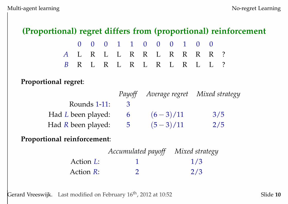
(Proportional) regret differs from (proportional) reinforcement

0 0 0 1 1 0 0 0 1 0 0

A L R L L R R L R R R R ?

B R L R L R L R L R L L ?

Proportional regret:

Payoff Average regret Mixed strategy

Rounds 1-11: 3

Had L been played: 6 (6 − 3)/11 3/5

Had R been played: 5 (5 − 3)/11 2/5

Proportional reinforcement:

Accumulated payoff Mixed strategy

Action L: 1 1/3

Action R: 2 2/3



Regret matching cast into a form similar to reinforcement

• Through reinforcement with an

aspiration level ut.

• Define the reinfor ement in rementfor every x in round t as

∆rtx =Def u(x, yt)− ut

• Define the propensities in round

t + 1 as

θt+1x =Def

[t

∑s=1

∆rtx

]

+

• This is like standard

reinforcement, but now all

actions in a given period are

reinforced, whether or not they

are actually played.

• Hypotheti al reinfor ement takes

into account virtual payoffs.

(Payoffs that never materialised.)

The vector ∆rt is a vector of

“virtual” reinforcements—gains

or losses relative to the current

average that that would have

materialised if a given action x

had been played at time t.



Adequacy of regret matching: proof outline

• Let

rtx =Def a umulated regret for not playing x, up to and including t

and

rtx =Def average regret for not playing x, up to and including t.

Let

[rtx]+ =Def rt

x ≥ 0 ? : rtx : 0

Dropping the subscript, x, is a way to denote the complete vector [rt]+ of

average regrets.

• The objective is to show that

limt→∞

sup [rt]+ = 0

with probability one. (The zero on the RHS again is a vector.)



Incremental regret

Suppose there are only two actions, “1” and “2,” say.

1. If 1 is executed at t + 1 then

• rt+11 will not change.

• rt+12 changes with u(2, yt+1) − u(1, yt+1).

2. If 2 is executed at t + 1 then

• rt+11 changes with u(1, yt+1) − u(2, yt+1).

• rt+12 will not change.

Thus, if αt+1 =Def u(2, yt+1)− u(1, yt+1) then incremental regret will be either

(0, αt+1) or (−αt+1, 0).

Suppose in round t + 1 a mixed strategy qt+1 = (qt+11 , qt+1

2 ) is played. Then

the expe ted in remental regret is

E[∆rt+1] = (qt+11 · 0 + qt+1

2 · −αt+1 , qt+11 · αt+1 + qt+1

2 · 0)



Decrease of expected regret

The objective is to find a (mixed) strategy g : H → ∆({1, 2}) such that

E[ [rt+1]+ | rt, . . . , r1] < rt (1)

because then again one of the martingale convergence theorems can be

applied to conclude limt→∞[rt]+ = 0. Since ∆E[rt+1] is known, we have

E[ rt+1 | rt, . . . , r1] = E[rt + ∆rt+1

t + 1| rt, . . . , r1]

=t

t + 1E[

rt

t| rt, . . . , r1] +

1

t + 1E[∆rt+1 | rt, . . . , r1]

=t

t + 1rt +

1

t + 1E[∆rt+1 | rt, . . . , r1]

=t

t + 1rt +

1

t + 1(−αt+1qt+1

2 , αt+1qt+11 )

The objective is to find a strategy qt+1 = g(ξt) such that Eq. (1) is satisfied.



A strategy q such that limt→∞[rt]+ = 0 : 1st attempt

Take qt1 = qt

2 = 1/2 for all t.

Then

E[rt1 + rt

2] = E[rt−1

1 + ∆rt1

t+

rt−12 + ∆rt

2

t]

= E[rt−1

1 + αt/2

t+

rt−12 − αt/2

t]

= E[rt−11 + rt−1

2 ]

Hence,

E[rt1 + rt

2] = 0,

so that limt→∞ rt1 + rt

2 = 0 with probability one.

However, the two regrets themselves may be unbounded and neutralise each

other. (Which is not what we want—we want all regrets to be non-positive.)



A strategy q such that limt→∞[rt]+ = 0 : 2nd attempt

• Each round t, choose an action

that would have minimised regret

in the previous round.

• Matching Pennies:

– Switch if wrong action in

previous round; else stay.

– Won’t work: suppose you

meet an opponent who

happens to switch every

round as well . . .

• Won’t work in general: your

corrections may by coincidence

be “in phase” with the path of

play of your opponent. Peyton

Young:

“Recall the no-regret must

hold even when Nature is

malevolent.”

(p. 26)



A strategy q such that limt→∞[rt]+ = 0 : E[∆rt+1] ⊥ rt+

• Recall: our objective is [rt]+ → 0.

• To this end, choose qt+1 such that

E[∆rt+1] ⊥ [rt]+

Thus:

E[∆rt+1]· rt+ = 0

⇔ (αt+1qt+12 , −αt+1qt+1

1 )· rt+ = 0

⇔ αt+1(qt+12 [rt

1]+ − qt+11 [rt

2]+) = 0

⇔ qt+11 : qt+1

2 = [rt1]+ : [rt

2]+

The last equation precisely

amounts to proportional regret

matching.

(Notice that αt+1 has left the

stage.)

• Boundary cases are obvious and

can be treated as follows:

– If rt1 > 0 and rt

2 ≤ 0, then let

qt+1 =Def (1, 0).

– If rt1 ≤ 0 and rt

2 > 0, then let

qt+1 =Def (0, 1).

– If all regret is non-positive,

then play a random action.



Stochastic dynamics of regret matching

• Expected incremental regret, E[∆rt+1] is

made orthogonal to the current regret,

independently of the unknown αt+1.

(Because A does not know what B

plays at t + 1, it is crucial that qt+1 does

not depend on αt+1.)

• E[rt+1] is a convex combination of rt+

and E[∆rt+1].

• Since E[∆rt+1] ⊥ rt+, E[rt+1] lies closer

to the non-positive orthant than does

rt+, provided t is large.

• rt+ → 0 follows from Bla kwell'sapproa hability theorem (PY, 2004, Ch. 4).

•[rt]+

•E[rt+1]

•E[∆rt+1]



Stochastic dynamics of regret matching

••••

•

••••

•

•

• •

•

••••

(Not sure whether the trace below the x-axis makes sense.)



Part III:

ǫ-Greedy Off-policy

Regret Matching



ǫ-Greedy regret matching (Foster & Vohra, 1998)

ǫ-greedy regret matching. Let ǫ > 0 small.

1. Explore. Play randomly ǫ% of the time. Only then compute regret.

2. Exploit. Else, play o�-poli y no regret.Define o�-poli y no regret for x in round t as

rtx =Def rt

x(E) − ut, where rtx(E) =

[

1

|Ex|∑

t∈Ex

u(xt, yt)

]

and

Ex = {t | A experimented in round t and played x }.

• Proposed as a forecasting heuristic by Foster and Vohra (1993).

• Can be conceived as a way of estimating regrets without knowing, or

having to care for, the actions of the opponent.



ǫ-Greedy regret matching (outline of proof)

Theorem (Foster et al., 1998). For all δ > 0 there exists an ǫ > 0 such that

ǫ-greedy regret matching has at most δ regret against all realisations of play.

By letting ǫ → 0 through time at a sufficiently slow rate, one can guarantee there is

no regret in the long run.

Proof . Suppose there are k different actions. Let et ∈ Rk such that

etx = ( A explores at t and chooses x ) ? 1 : 0.

For each action i

Pr(xt = i | A explores at round t) = 1/k.

Hence,

E[et] = (ǫ/k, . . . , ǫ/k).




Define

ztx =Def

(k

ǫ· et

x· u(x, yt)

)

− u(x, yt).

In words, ztx is the difference between (properly magni�ed) empiri al payo� for x

and ( orre t but) virtual payo� for x. Hence,

E[ztx] = E

[(k

ǫ· et

x· u(x, yt)

)

− u(x, yt)

]

= E

[k

ǫ· et

x· u(x, yt)

]

− E[u(x, yt)]

=k

ǫ· E[et

x]· E[u(x, yt)] − E[u(x, yt)] (et and ut are independent)

=k

ǫ·

ǫ

k· E[u(x, yt)] − E[u(x, yt)]

= 0.




Strong law of large numbers for dependent random variables. Let {wt}t

be a bounded sequence of possibly dependent random variables in Rk. Let

zt = E[ wt |wt−1, wt−2, . . . , w1 ] − wt, and zt the average of the zt’s. Then

limt→∞ zt = 0 with probability one.

We have

ztx =Def

(k

ǫ· et

x· u(x, yt)

)

− u(x, yt).

and

E[ztx] = 0.

If

zt =Def average of zs, s ≤ t

then it follows from the above strong law of large numbers that limt→∞ zt = 0

with probability one. (PY refers to Loève, 1978, Book II, Th. 32.E.1.)



Estimated vs. true regret

Now write ztx as follows (!):

ztx =

1

t

k

ǫ

t

∑s=1

esx· u(x, ys)− ut

︸︷︷︸

regret estimated

in experimentation

−1

t

t

∑s=1

u(x, ys) − ut

︸︷︷︸

proper regret

a) The first term approaches regret

as estimated in experimental

rounds, since ǫt/k → ∞ when

t → ∞.

b) The second term is true regret.

c) Since we know limt→∞ zt = 0,

empirical regret converges to true

regret almost certainly.

d) (1 − ǫ)% of the time A plays

estimated regret true regret.

e) ǫ% of the time A explores, and

strategies are within 1 + 1 = 2.

f) In the long run, play is within 2ǫ

of minimal regret.

g) If ǫ is set to δ/2, the error

remains within 2 · δ/2. �



Literature

• No-regret learning can be traced

to Bla kwell's approa habilitytheorem and Hannan’s notion ofuniversal onsisten y.

• The diagram on regret matching

is taken from Peyton Young, and

Foster and Vohra (who formulate

the problem from a decision

theoretic point of view).

• The regret-matching algorithm

and the analysis of its

convergence to correlated

equilibria (a generalisation of

Nash equilibria) is given by Hart

and Mas-Colell.

Blackwell, D. (1956). “Controlled random walks”.Proc. of the Int. Congress of Mathematicians, North-Holland Publishing Comp., pp. 336-338.

Hannan, J. F. (1957). “Approximation to Bayes riskin repeated plays”. Contributions to the Theory ofGames, 3, pp. 97-139.

Hart, S., and Mas-Colell, A. (2000). “A simple adap-tive procedure leading to correlated equilibrium”.Econometrica, 68, pp. 1127-1150.

Foster, D., and Vohra, R. (1999). “Regret in the on-line decision problem”. GEB: Games and EconomicBehavior, 29, pp. 7-36.



What next?

• Fictitious Play. Monitor actions of opponent(s) and play a best response to

most frequent actions. As opposed to no-regret, fictitious play is

interested in the opponent's behaviour to predict future play.

• Smoothed fictitious play. With fictitious play, the probability to play

sub-optimal responses is zero. Smoothed fictitious play plays sub-optimal

responses proportional to their expected payoff, given opponents’ play.

• Conditional no-regret. Conditions on particular actions. There is regret if

there is a pair of actions (x, x′) such that, with hindsight, playing x′ was

better than playing x.

• Satisficing Play. While payoffs equal or supersede the average of past

payoffs, keep playing the same action.


multi-agent learning no-regret learning - utrecht university · multi-agent learning no-regret...

Documents