mse3 ch12 airmasses & fronts · 389 chapter 12 airmasses & fronts 12 a high-pressure...
TRANSCRIPT

389
Chapter 12
airMasses & Fronts
12 A high-pressure center, or high (H), often contains an airmass of well-defined characteristics, such as cold
temperatures and low humidity. When different airmasses finally move and interact, their mutual border is called a front, named by analogy to the battle fronts of World War I. Fronts are usually associated with low-pressure centers, or lows (L). Two fronts per low are most common, although zero to four are also observed. In the Northern Hemisphere, these fronts often ro-tate counterclockwise around the low center like the spokes of a wheel (Fig. 12.1), while the low moves and evolves. Fronts are often the foci of clouds, low pressure, and precipitation. In this chapter you will learn the characteristics of anticyclones (highs). You will see how anticy-clones are favored locations for airmass formation. Covered next are fronts in the bottom, middle, and top of the troposphere. Factors that cause fronts to form and strengthen are presented. This chapter ends with a special type of front called a dry line.
Contents
Anticyclones or Highs 390Characteristics & Formation 390Vertical Structure 391
Airmasses 391Creation 392Movement 397Modification 397
Surface Fronts 399Horizontal Structure 400Vertical Structure 403
Geostrophic Adjustment – Part 3 404Winds in the Cold Air 404Winds in the Warm Over-riding Air 407Frontal Vorticity 407
Frontogenesis 408Kinematics 408Thermodynamics 411Dynamics 411
Occluded Fronts and Mid-tropospheric Fronts 413
Upper-tropospheric Fronts 414
Drylines 416
Summary 417Threads 418
Exercises 418Numerical Problems 418Understanding & Critical Evaluation 419Web-Enhanced Questions 421Synthesis Questions 423
Copyright © 2011, 2015 by Roland Stull. Meteorology for Scientists and Engineers, 3rd Ed.
Figure 12.1Idealized surface weather map (from the Weather Reports & Map Analysis chapter) for the N. Hemisphere showing high (H) and low (L) pressure centers, isobars (thin lines), a warm front (heavy solid line with semicircles on one side), a cold front (heavy solid line with triangles on one side), and a trough of low pressure (dashed line). Vectors indicate near-surface wind. cP indicates a continental polar airmass; mT indicates a maritime tropical airmass.
“Meteorology for Scientists and Engineers, 3rd Edi-tion” by Roland Stull is licensed under a Creative Commons Attribution-NonCommercial-ShareAlike
4.0 International License. To view a copy of the license, visit http://creativecommons.org/licenses/by-nc-sa/4.0/ . This work is available at http://www.eos.ubc.ca/books/Practical_Meteorology/ .

390 CHAPTEr 12 AirMASSES & FrONTS
antiCyClones or highs
Characteristics & Formation High-pressure centers, or highs, are identified on constant altitude (e.g., sea-level) weather maps as regions of relative maxima in pressure. The loca-tion of high-pressure center is labeled with “H” (Fig. 12.2a). High centers can also be found on upper-air isobaric charts as relative maxima in geopotential height (see the Dynamics chapter, Fig. 10.2). When the pressure field has a relative maximum in only one direction, such as east-west, but has a horizontal pressure-gradient in the other direction, this is called a high-pressure ridge (Fig. 12.2b). The ridge axis is labeled with a zigzag line. The column of air above the high center contains more air molecules than neighboring columns. This causes more weight due to gravity (see Chapter 1), which is expressed in a fluid as more pressure. Above a high center is often downward mo-tion (subsidence) in the mid-troposphere, and horizontal spreading of air (divergence) near the surface (Fig. 12.3a). Subsidence impedes cloud de-velopment, leading to generally clear skies and fair weather. Winds are also generally calm or light in highs, because gradient-wind dynamics of highs re-quire weak pressure gradients near the high center (see the Dynamics chapter). The diverging air near the surface spirals out-ward due to the weak pressure-gradient force. Coriolis force causes it to rotate clockwise (anticy-clonically) around the high-pressure center in the Northern Hemisphere (Fig. 12.2a), and opposite in the Southern Hemisphere. For this reason, high-pressure centers are called anticyclones. Downward advection of dry air from the upper troposphere creates dry conditions just above the boundary layer. Subsidence also advects warmer potential temperatures from higher in the tropo-sphere. This strengthens the temperature inversion that caps the boundary layer, and acts to trap pollut-ants and reduce visibility near the ground. Subsiding air cannot push through the capping inversion, and therefore does not inject free-atmo-sphere air directly into the boundary layer. Instead, the whole boundary layer becomes thinner as the top is pushed down by subsidence (Fig. 12.3a). This can be partly counteracted by entrainment of free at-mosphere air if the boundary layer is turbulent, such as for a convective mixed layer during daytime over land. However, the entrainment rate is controlled by turbulence in the boundary layer (see the Atmos. Boundary Layer chapter), not by subsidence.
Figure 12.3(a) Left: vertical circulation above a surface high-pressure center in the bottom half of the troposphere. Black dashed line marks the initial capping inversion at the top of the boundary layer. Grey dashed line shows the top later, assuming no turbulent entrainment into the boundary layer. Right: idealized profile of potential temperature, θ, initially (black line) and later (grey). The boundary-layer depth zi is on the order of 1 km, and the potential-temperature gradient above the boundary layer is rep-resented by γ.(b) Tilt of high-pressure ridge westward with height, toward the warmer air. Thin lines are height contours of isobaric surfaces. Ridge amplitude is exaggerated in this illustration.
Figure 12.2Examples of isobars plotted on a sea-level pressure map. (a) High-pressure center. (b) High-pressure ridge in N. Hemisphere mid-latitudes. Vectors show surface wind directions.

r. STULL • METEOrOLOGy FOr SCiENTiSTS AND ENGiNEErS 391
Five mechanisms support the formation of highs at the Earth’s surface:
• Global Circulation: Planetary-scale, semi-per-manent highs predominate at 30° and 90° latitudes, where the global circulation has downward motion (see the Global Circulation chapter). The subtropi-cal highs centered near 30° North and South lati-tudes are 1000-km-wide belts that encircle the Earth. Polar highs cover the Arctic and Antarctic. These highs are driven by the global circulation that is re-sponding to differential heating of the Earth. Al-though these highs exist year round, their locations shift slightly with season.
• Monsoons: Quasi-stationary, continental-scale highs form over cool oceans in summer and cold continents in winter (see the Global Circula-tion chapter). They are seasonal (i.e., last for several months), and form due to the temperature contrast between land and ocean.
• Transient Rossby waves: Surface highs form at mid-latitudes, east of high-pressure ridges in the jet stream, and are an important part of mid-latitude weather variability (see the Global Circulation and Extratropical Cyclone chapters). They often exist for several days.
• Thunderstorms: Downdrafts from thunder-storms (see the Thunderstorm chapters) create meso-highs roughly 10 to 20 km in diameter at the surface. These might exist for minutes to hours.
• Topography/Surface-Characteristics: Meso-highs can also form in mountains due to blocking or channeling of the wind, mountain waves, and thermal effects (anabatic or katabatic winds) in the mountains. Sea-breezes or lake breezes can also cre-ate meso-highs in parts of their circulation. (See the Local Winds chapter.)
The actual pressure pattern at any location and time is a superposition of all these phenomena.
Vertical structure The location difference between surface and up-per-tropospheric highs (Fig. 12.3b) can be explained using gradient-wind and thickness concepts. Because of barotropic and baroclinic instability, the jet stream meanders north and south, creating troughs of low pressure and ridges of high pres-sure, as discussed in the Global Circulation chapter. Gradient winds blow faster around ridges and slower around troughs, assuming identical pressure gradients. The region east of a ridge and west of a
trough has fast-moving air entering from the west, but slower air leaving to the east. Thus, horizontal convergence of air at the top of the troposphere adds more air molecules to the whole tropospheric col-umn at that location, causing a surface high to form east of the upper-level ridge. West of surface highs, the anticyclonic circula-tion advects warm air from the equator toward the poles (Figs. 12.2a & 12.3b). This heating west of the surface high causes the thickness between isobaric surfaces to increase, as explained by the hypsometric equation. Isobaric surfaces near the top of the tro-posphere are thus lifted to the west of the surface high. These high heights correspond to high pres-sure aloft; namely, the upper-level ridge is west of the surface high. The net result is that high-pressure regions tilt westward with increasing height (Fig. 12.3b). In the Extratropical Cyclone chapter you will see that deep-ening low-pressure regions also tilt westward with increasing height, at mid-latitudes. Thus, the mid-lat-itude tropospheric pressure pattern has a consistent phase shift toward the west as altitude increases.
airMasses
An airmass is a widespread (of order 1000 km wide) body of air in the bottom third of the tropo-sphere that has somewhat-uniform characteristics. These characteristics can include one or more of: temperature, humidity, visibility, odor, pollen con-centration, dust concentration, pollutant concentra-tion, radioactivity, cloud condensation nuclei (CCN) activity, cloudiness, static stability, and turbulence. Airmasses are usually classified by their temper-ature and humidity, as associated with their source regions. These are usually abbreviated with a two-letter code. The first letter, in lowercase, describes the humidity source. The second letter, in upper-
Solved Example A “cA“ airmass has what characteristics?
SolutionGiven: cA airmass. Find: characteristics
Use Table 12-1: cA = continental ArcticCharacteristics: Dry and very cold.
Check: Agrees with Fig. 12.4.Discussion: Forms over land in the arctic, under the polar high. In Great Britain, the same airmass is la-beled as Ac.
392 CHAPTEr 12 AirMASSES & FrONTS
case, describes the temperature source. Table 12-1 shows airmass codes. [CAUTION: In Great Britain, the two letters are reversed.] Examples are maritime Tropical (mT) air-masses, such as can form over the Gulf of Mexico, and continental Polar (cP) air, such as can form in winter over Canada. After the weather pattern changes and the air-mass is blown away from its genesis region, it flows over surfaces with different relative temperatures. Some organizations append a third letter to the end of the airmass code, indicating whether the moving airmass is (w) warmer or (k) colder than the under-lying surface. This coding helps indicate the likely static stability of the air and the associated weather. For example, “mPk” is humid cold air moving over warmer ground, which would likely be statically unstable and have convective clouds and showers.
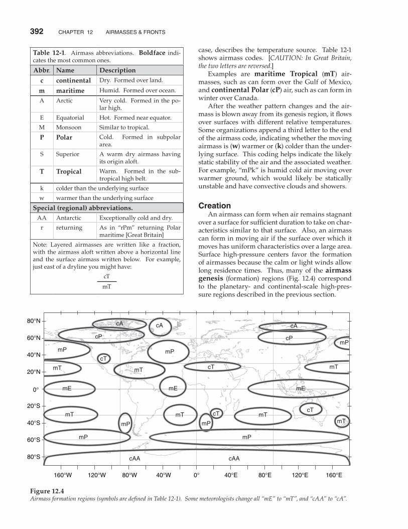
Creation An airmass can form when air remains stagnant over a surface for sufficient duration to take on char-acteristics similar to that surface. Also, an airmass can form in moving air if the surface over which it moves has uniform characteristics over a large area. Surface high-pressure centers favor the formation of airmasses because the calm or light winds allow long residence times. Thus, many of the airmass genesis (formation) regions (Fig. 12.4) correspond to the planetary- and continental-scale high-pres-sure regions described in the previous section.
Figure 12.4Airmass formation regions (symbols are defined in Table 12-1). Some meteorologists change all “mE” to “mT”, and “cAA” to “cA”.
Table 12-1. Airmass abbreviations. Boldface indi-cates the most common ones.
Abbr. Name Description
c continental Dry. Formed over land.
m maritime Humid. Formed over ocean.
A Arctic Very cold. Formed in the po-lar high.
E Equatorial Hot. Formed near equator.
M Monsoon Similar to tropical.
P Polar Cold. Formed in subpolar area.
S Superior A warm dry airmass having its origin aloft.
T Tropical Warm. Formed in the sub-tropical high belt.
k colder than the underlying surface
w warmer than the underlying surface
Special (regional) abbreviations.AA Antarctic Exceptionally cold and dry.
r returning As in “rPm” returning Polar maritime [Great Britain]
Note: Layered airmasses are written like a fraction, with the airmass aloft written above a horizontal line and the surface airmass written below. For example, just east of a dryline you might have:
cT
mT

r. STULL • METEOrOLOGy FOr SCiENTiSTS AND ENGiNEErS 393
Airmasses form as boundary layers. During their residence over a surface, the air is modified by processes including radiation, conduction, diver-gence, and turbulent transport between the ground and the air.
Warm Airmass Genesis When cool air moves over a warmer surface, the warm surface modifies the bottom of the air to cre-ate an evolving, convective mixed layer (ML). Turbulence — driven by the potential temperature difference ∆θs between the warm surface θsfc and the cooler airmass θML — causes the ML depth zi to initially increase (Fig. 12.5). This is the depth of the new airmass. A heat flux from the warm surface into the air causes θML to warm toward θsfc. θML is the temperature of the new airmass as it warms. Synoptic-scale divergence β and subsidence ws, which is expected in high-pressure airmass-genesis regions, oppose the ML growth. Changes within the new airmass are rapid at first. But as airmass temperature gradually approaches surface tempera-ture, the turbulence diminishes and so does the rate of ML depth increase. Eventually, the ML depth be-gins to decrease (Fig. 12.5) because the reduced tur-bulence (trying to increase the ML thickness) cannot counteract the relentless subsidence. A “toy model” describing the atmospheric boundary-layer processes that create a warm air-mass is given in the Focus Box. The nearby Solved Example box uses this toy model to find the evolu-tion of the warm airmass depth (i.e., the ML depth zi) and its potential temperature θML evolution. This is the solution that was plotted in Fig. 12.5. The e-folding time (see Chapter 1) for the θML to approach θsfc is surprisingly constant — about 1 to 2 days. As a result, creation of this warm tropical airmass is nearly complete after about a week. That is how long it takes until the airmass temperature nearly equals the surface temperature (Fig. 12.5). The time τ to reach the peak ML thickness is typi-cally about 1 to 4 days (see another Focus box).
Cold Airmass Genesis When air moves over a colder surface such as arc-tic ice, the bottom of the air first cools by conduction, radiation, and turbulent transfer with the ground. Turbulence intensity then decreases within the in-creasingly statically-stable boundary layer, reducing the turbulent heat transport to the cold surface. However, direct radiative cooling of the air, both upward to space and downward to the cold ice sur-face, chills the air at rate 2°C/day (averaged over a 1 km thick boundary layer). As the air cools below the dew point, water-droplet clouds form. Continued radiative cooling from cloud top allows ice crystals
Figure 12.5Genesis of a warm airmass after cold air comes to rest over a warmer surface. This is an example based on toy-model equa-tions in the Focus Box. Airmass potential temperature is θML and depth is zi. Imposed conditions for this case-study example are: large-scale divergence β = 10–6 s–1, potential temperature gradient in vertical γo = 3.3 K/km, initial near-surface air po-tential temperature θML = θo = 10°C, and surface temperature θsfc = 20°C.
on Doing sCienCe • Math Clarity
In math classes, you might have learned how to combine many small equations into a single large equation that you can solve. For meteorology, al-though we could make such large single-equation combinations, we usually cannot solve them. So there is no point in combining all the equa-tions. Instead, it is easier to see the physics involved by keeping separate equations for each physical pro-cess. An example is the toy model given in the Focus Box on the next page for warm airmass genesis. Even though the many equations are coupled, it is clearer to keep them separate.

394 CHAPTEr 12 AirMASSES & FrONTS
FoCUs • Warm airmass genesis
Modeling warm airmass creation (genesis) is an exercise in atmospheric boundary-layer (ABL) evolu-tion. Since we do not cover ABLs in detail until a later chapter, the details are relegated to this Focus Box. You can safely skip them now, and come back later after you have studied ABLs. Define a relative potential temperature θ based on a reference height (z) at the surface (z = 0). Namely, θ ≈ T + Γd · z, where Γd = 9.8 °C/km is the dry adiabatic lapse rate.
Suppose that a cool, statically stable layer of air initially (subscript o) has a near-surface temperature of θo and a linear potential-temperature gradient γo = γ = ∆θ/∆z before it comes to rest over a warm surface of temperature θsfc (see Fig. above). We want to pre-dict the time evolution of the depth (zi) and potential temperature (θML) of this new airmass. Because this airmass is an ABL, we can use boundary-layer equa-tions to predict zi (the height of the convective mixed-layer ,ML), and θML (the ML potential temperature). ML depth increases by amount ∆zie during a time interval ∆t due to thermodynamic encroach-ment (i.e., warming under the capping sounding). This is an entrainment process that adds air to the ML through the ML top. Large scale divergence β = +∆ / ∆ ∆ / ∆U x V y removes air horizontally from the ML and causes a subsidence velocity of magni-tude ws at the ML top: w zs i= β· * (7)
Thus, a change in ML depth results from the competi-tion of these two terms: z z z w ti i ie s= + −* ∆ ·∆ (12)
where the asterisk * indicates a value from the previ-ous time step. The amount of heat ∆Q (as an incremental accu-mulated kinematic heat flux) transferred from the warm surface to the cooler air during time interval ∆t under light-wind conditions depends on the tempera-ture difference at the surface ∆θs and the intensity of turbulence, as quantified by a buoyancy velocity scale wb: ∆ · ·∆ ·∆Q b w tb s= θ (10)
where b = 5x10⁻⁴ (dimensionless) is a convective heat transport coefficient (see the Heat chapter). (continues in next column)
FOCUS (continuation) The buoyancy velocity scale is:
wg
zbML
i s= ∆
θ
θ**
/
· ·1 2
(9)
where |g| = 9.8 m/s2 is gravitational acceleration. That heat goes to warming θML, which by geom-etry adds a trapezoidal area under the γ curve :
∆·∆ *
/*z
Qz zie i i= + ( )
−2 2
1 2
γ (11)
Knowing the entrainment rate, we get ∆θML geo-metrically from where it intercepts the γ curve: θ θ γML ML iez= +* ·∆ (13)
With this new ML temperature, we can update the surface temperature difference ∆ = −θ θ θs sfc ML
* (8)
Knowing the large-scale divergence, we can also up-date the potential temperature profile in the air above the ML: γ γ β= o t·exp( · ) (6)
All that remains is to update the time variable: t = t* + ∆t (5)
You might have noticed that some of the equations above are initially singular, when the ML has zero depth. So, for the first small time step (∆t ≈ 6 minutes = 360 s), you should use the following special equa-tions in the following order: t = ∆t (1)
∆ = −θ θ θs sfc o (2)
zb t g
i so o
=
∆ ·· ·∆
·/ /
θγ θ
21 2 2 3
(3)
θ θ γML o o iz= + · (4)
Then, for all the subsequent time steps, use the set of equations (5 to 13 in the order as numbered) to find the resulting ML evolution. Repeat eqs. (5 to 13) for each subsequent step. As the solution begins to change more gradually, you may use larger time steps ∆t. The result is a toy model that describes warm air-mass formation as an evolving convective boundary layer. The solved example on the next page shows how this can be done with a computer spreadsheet. First, you need to specify the imposed constants γo , θo, β and θsfc. Next, initialize the values of: γ = γo , zi = 0, and θML = θo at t = 0 . Then, solve the equations for the first step. Finally, continue iterating for subse-quent time steps to simulate warm airmass genesis. These simulations show that greater divergence causes a shallower ML that can warm faster. Greater static stability in the ambient environment reduces the peak ML depth.

r. STULL • METEOrOLOGy FOr SCiENTiSTS AND ENGiNEErS 395
Solved Example (§) Air of initial ML potential temperature 10°C comes to rest over a 20°C sea surface. Divergence is 10–6 s–1, and the initial ∆θ/∆z = γ = 3.3 K/km. Find and plot the warm airmass evolution of potential temperature and depth.
SolutionGiven: θo = 10°C = 283K, θsfc = 20°C, γo = 3.3 K/km, β = 10–6 s–1. Find: θML(t) = ? °C, zi(t) = ? m
For the first time step of ∆t = 6 min (=360 s), use eqs. (1 to 4 from the Focus Box on the previous page). For subsequent steps, repeatedly use eqs. (5 to 13 from that same Focus Box).
t(s)
t(d)
γ(K/m)
ws(m/s)
∆θs (°C)
wb(m/s)
∆Q(K·m)
∆zie(m)
zi(m)
θML (°C)
0 0.000 0 10360 0.004 10 74 10.2720 0.008 0.00330 0.00007 9.75 5.0 8.8 29.8 104 10.31080 0.013 0.00330 0.00010 9.66 5.9 10.3 26.4 131 10.41440 0.017 0.00330 0.00013 9.57 6.6 11.3 24.0 155 10.5. . .
259200 3.00 0.00428 0.00179 2.41 12.0 104.3 13.6 1789 17.7270000 3.13 0.00432 0.00179 2.35 11.9 150.8 19.4 1789 17.7280800 3.25 0.00437 0.00179 2.26 11.7 142.8 18.2 1788 17.8
. . .1684800 19.50 0.01779 0.00057 0.14 1.6 4.9 0.5 542 19.91728000 20.00 0.01858 0.00054 0.13 1.5 4.4 0.4 519 19.9
Sample results from the computer spreadsheet are shown above. The final answer is plotted in Fig. 12.5.
Check: Units OK. Physics OK. Fig. 12.5 reasonable.Discussion: I used small time steps of ∆t = 6 minutes initially, and then as ∆zie became smaller, I gradually increased past ∆t = 3 h to ∆t = 12 h. The figure shows rapid initial modification of the cold, statically stable airmass toward a warm, unstable airmass. Maximum zi is reached in about τ = 3.06 days (see Focus box), in agreement with Fig. 12.5.
FoCUs • time of Max airmass thickness
The time τ to reach the peak ML thickness for warm airmass genesis is roughly
τθ
β γ β τ≈
c
g eo
o·
· · · ·
/1 3
(c)
where c = 140 (dimensionless), and the other variables are defined in the text. τ is typically about 1 to 4 days. Any further lingering of the airmass over the same surface temperature results in a loss of airmass thick-ness due to divergence. Equation (c) is an implicit equation; namely, you need to know τ in order to solve for τ. Although this equation is difficult to solve analytically, you can iter-ate to quickly converge to a solution in about 5 steps in a computer spreadsheet. Namely, start with τ = 0 as the first guess and plug into the right side of eq. (c). Then solve for τ on the left side. For the next iteration, take this new τ and plug it in on the right, and solve for an updated τ on the left. Repeat until the value of τ converges to a solution; namely, when ∆τ/τ < ε for ε = 0.01 or smaller.
Solved Example (§) For the conditions of the previous solved example, find the time τ that estimates when the new warm air-mass has maximum thickness.
SolutionGiven: θo = 10°C = 283K, θsfc = 20°C, γo = 3.3 K/km, β = 10–6 s–1. Find: τ = ? days
Use eq. (c) from the Focus Box at left. Start with τ = 0. The first iteration is:
τ = −140283
9 8 10 0 00336·( . )·( )·( . )·
K
m/s s K/m2 -1 e00
1 3
/
= 288498 s = 3.339 daysSubsequent iterations give: τ = 3.033 -> 3.060 -> 3.057 -> 3.058 -> 3.058 days
Check: Units OK. Physics OK. Agrees with Fig. 12.5.Discussion: Convergence was quick. From Fig. 12.5, the actual time of this peak thickness was between 3 and 3.125 days, so eq. (c) does a reasonable job.

396 CHAPTEr 12 AirMASSES & FrONTS
to grow at the expense of evaporating liquid drop-lets, changing the cloud into an ice cloud. Radiative cooling from cloud top creates cloudy “thermals” of cold air that sink, causing some turbu-lence that distributes the cooling over a deeper layer. Turbulent entrainment of air from above cloud top down into the cloud allows the cloud top to rise, and deepens the incipient airmass (Fig. 12.6). The ice crystals within this cloud are so few and far between that the weather is described as cloud-less ice-crystal precipitation. This can create some spectacular halos and other optical phenomena in sunlight (see the Optics chapter), including spar-kling ice crystals known as diamond dust. Never-theless, infrared radiative cooling in this cloudy air is much greater than in clear air, allowing the cool-ing rate to increase to 3°C/day over a layer as deep as 4 km. During the two-week formation of this conti-nental-polar or continental-arctic airmass, most of the ice crystals precipitate out leaving a thin-ner cloud of 1 km depth. Also, subsidence within the high pressure also reduces the thickness of the cloudy airmass and causes some warming to par-tially counteract the radiative cooling. Above the final fog layer is a nearly isothermal layer of air 3 to 4 km thick that has cooled about 30°C. Final air-mass temperatures are often in the range of –30 to –50 °C, with even colder tempera-tures near the surface. While the Arctic surface consists of relatively flat sea-ice (except for Greenland), the Antarctic has mountains, high ice-fields, and significant surface to-pography (Fig. 12.7). As cold air forms by radiation, it can drain downslope as a katabatic wind (see the Local Winds chapter). Steady winds of 10 m/s are common in the Antarctic interior, with speeds of 50 m/s along some of the steeper slopes. As will be shown in the Local Winds chapter, the buoyancy force per unit mass on a surface of slope ∆z/∆x translates into a quasi-horizontal slope-force per mass of:
F
m
g
Tzx
x S
e=
∆ ∆∆
··
θ •(12.1)
F
m
g
Tzy
y S
e=
∆ ∆∆
··
θ •(12.2)
where |g| = 9.8 m·s–2 is gravitational acceleration, and ∆θ is the potential-temperature difference be-tween the draining cold air and the ambient air above. The ambient-air absolute temperature is Te. The sign of these forces should be such as to ac-celerate the wind downslope. The equations above work when the magnitude of slope ∆z/∆x is small,
Solved Example Find the slope force per unit area acting on a katabatic wind of temperature –20°C with ambient air temperature 0°C. Assume a slope of ∆z/∆x = 0.1 .
SolutionGiven: ∆θ = 20 K, Te = 273 K, ∆z/∆x = 0.1Find: Fx S/m = ? m·s–2
Use eq. (12.1):
F
mx S =
−( . · )·( )·( . )
9 8 200 1
m s K273K
2
= 0.072 m·s–2
Check: Units OK. Physics OK.Discussion: This is two orders of magnitude greater than the typical synoptic forces (see the Dynamics chapter). Hence, drainage winds can be strong.
Figure 12.6Genesis of a continental-polar air mass over arctic ice. The cloud/fog regions are shaded.
Figure 12.7Cold katabatic winds draining from Antarctica.

r. STULL • METEOrOLOGy FOr SCiENTiSTS AND ENGiNEErS 397
because then ∆z/∆x = sin(α), where α is the slope angle of the topography. The katabatic wind speed in the Antarctic also depends on turbulent drag force against the ice sur-face, ambient pressure-gradient force associated with synoptic weather systems, Coriolis force, and turbulent drag caused by mixing of the draining air with the stationary air above it. At an average drain-age velocity of 5 m/s, air would need over 2 days to move from the interior to the periphery of the conti-nent, which is a time scale on the same order as the inverse of the Coriolis parameter. Hence, Coriolis force cannot be neglected. Katabatic drainage removes cold air from the genesis regions and causes turbulent mixing of the cold air with warmer air aloft. The resulting cold-air mixture is rapidly distributed toward the outside edges of the antarctic continent. One aspect of the global circulation is a wind that blows around the poles. This is called the po-lar vortex. Katabatic removal of air from over the antarctic reduces the troposphere depth, enhancing the persistence and strength of the antarctic polar vortex due to potential vorticity conservation.
Movement Airmasses do not remain stationary over their birth place forever. After a week or two, a transient change in the weather pattern can push the airmass toward new locations. When airmasses move, two things can happen:(1) As the air moves over surfaces with different characteristics, the airmass begins to change. This is called airmass modification, and is described in the next subsection.(2) An airmass can encounter another airmass. The boundary between these two airmasses is called a front, and is a location of strong gradients of tem-perature, humidity, and other airmass characteris-tics. Fronts are described in detail later. Tall mountain ranges can strongly block or channel the movement of airmasses, because air-masses occupy the bottom of the troposphere. Fig. 12.8 shows a simplified geography of major moun-tain ranges. For example, in the middle of North America, the lack of any major east-west mountain range allows the easy movement of cold polar air from Canada toward warm humid air from the Gulf of Mexico. This sets the stage for strong storms (see the Extra-tropical Cyclone chapter and the chapters on Thun-derstorms). The long north-south barrier of mountains (Rock-ies, Sierra Nevada, Cascades, Coast Range) along the west coast of North America impedes the easy entry of Pacific airmasses toward the center of that conti-
nent. Those mountains also help protect the west coast from the temperature extremes experienced by the rest of the continent. In Europe, the mountain orientation is the op-posite. The Alps and the Pyrenees are east-west mountain ranges that inhibit movement of Mediter-ranean airmasses from reaching northward. The lack of major north-south ranges in west and central Europe allows the easy movement of maritime air-masses from the Atlantic to sweep eastward, bring-ing cool wet conditions. One of the greatest ranges is the Himalaya Mountains, running east-west between India and China. Maritime tropical airmasses moving in from the Indian Ocean reach these mountains, causing heavy rains over India during the monsoon. The same mountains block the maritime air from reach-ing further northward, leaving a very dry Tibetan Plateau and Gobi Desert in its rain shadow. The discussion above focused on blocking and channeling by the mountains. In some situations air can move over mountain tops (Fig. 12.9). When this happens, the airmass is strongly modified, as described next.
Modification As an airmass moves from its origin, it is modi-fied by the new landscapes under it. For example, a polar airmass will warm and gain moisture as it moves equatorward over warmer vegetated ground. Thus, it gradually loses its original identity.
Via Surface Fluxes Heat and moisture transfer at the surface can be described with bulk-transfer relationships such as eq. (3.34). If we assume for simplicity that wind-induced turbulence creates a well-mixed airmass of quasi-constant thickness zi, then the change of
Figure 12.8Locations of major mountain ranges (black lines), lesser ranges (grey lines), and large plateaus of land or ice (black ovals).

398 CHAPTEr 12 AirMASSES & FrONTS
airmass potential temperature θML with travel-dis-tance ∆x is:
∆
∆≈
−θ θ θML H sfc ML
ix
C
z
·( ) (12.3)
where CH ≈ 0.01 is the bulk-transfer coefficient for heat (see the chapters on Heat and on the Atmo-spheric Boundary Layer). If the surface temperature is horizontally homo-geneous, then eq. (12.3) can be solved for the airmass temperature at any distance x from its origin:
θ θ θ θML sfc sfc ML oH
i
C xz
= − − −
( )·exp· (12.4)
where θML o is the initial airmass potential tempera-ture at location x = 0.
Solved Example A polar airmass with initial θ = –20°C and depth = 500 m moves southward over a surface of 0°C. Find the initial rate of temperature change with distance.
SolutionGiven: θML = –20°C, θsfc = 0°C, zi = 500 mFind: ∆θML /∆x = ? °C/km. Assume no mountains.
Use eq. (12.3):
∆
∆≈
− −θMLx
( . )·[ ( )]( )
0 01 0 20500° °C C
m = 0.4 °C/km
Check: Units OK. Physics OK.Discussion: Neither this answer nor eq. (12.4) de-pend on wind speed. While faster speeds give faster position change, they also cause greater heat transfer to/from the surface (eq. 3.34). These 2 effects cancel.
Solved Example An mP airmass initially has T = 5°C & RH = 100%. Use a thermo diagram to find T & RH at: 1 Olympic Mtns (elevation ≈ 1000 m), 2 Puget Sound (0 m), 3 Cas-cade Mtns (1500 m), 4 the Great Basin (500 m), 5 Rocky Mtns (2000 m), 6 the western Great Plains (1000 m).
SolutionGiven: Elevations from west to east (m) = 0, 1000, 0, 1500, 500, 2000, 1000 Initially RH=100%. Thus Td = T = 5°CFind: T (°C) & RH (%) at surface locations 1 to 6.Assume: All condensation precipitates out. No additional heat or moisture transfer from the surface. Start with air near sea level, where PSL = 100 kPa.
Use Fig. 12.9 and an emagram from the Stability chapter. On the thermo diagram, the air parcel follows the following route: 0 - 1 - 2 - 1 - 3 - 4 - 3 - 5 - 6. Initially (point 0), Td = T = 5°C. Because this air is already saturated, it would follow a saturated adiabat from point 0 to point 1 at z = 1 km, where the still-satu-rated air has Td = T = –1°C. If all condensates precipitate out, then air would de-scend dry adiabatically (with Td following an isohume) from point 1 to 2, giving T = 9°C and Td = 1°C. When this unsaturated air rises, it first does so dry adiabatically until it reaches its LCL at point 1. This now-cloudy air continues to rise toward point 3 moist adiabatically, where it has Td = T = –4°C. Etc.
Results, where Index = circled numbers in Fig above.
Index z (km) T (°C) Td (°C) RH (%)0 0 5 5 1001 1 –1 –1 1002 0 9 1 553 1.5 –4 –4 1004 0.5 6 –2 545 2 –7 –7 1006 1 2 –6 53
Check: Units OK. Physics OK. Figure OK.Discussion: The airmass has lost its maritime iden-tity by the time it reaches the Great Plains, and little moisture remains. Humidity for rain in the plains comes from the southeast (not from the Pacific).
Figure 12.9Modification of a Pacific airmass by flow over mountains in the northwestern USA. (Numbers are used in the solved example.)

r. STULL • METEOrOLOGy FOr SCiENTiSTS AND ENGiNEErS 399
Via Flow Over Mountains If an airmass is forced to rise over mountain ranges, the resulting condensation, precipitation, and latent heating will dry and warm the air. For example, an airmass over the Pacific Ocean near the northwestern USA is often classified as maritime polar (mP), because it is relatively cool and humid. As the prevailing westerly winds move this air-mass over the Olympic Mountains (a coastal moun-tain range), the Cascade Mountains, and the Rocky Mountains, there is substantial precipitation and la-tent heating (Fig. 12.9).
sUrFaCe Fronts
Surface fronts mark the boundaries between air-masses at the Earth’s surface. They usually have the following attributes:
• strong horizontal temperature gradient • strong horizontal moisture gradient • strong horizontal wind gradient • strong vertical shear of the horizontal wind • relative minimum of pressure • high vorticity • confluence (air converging horizontally) • clouds and precipitation • high static stability • kinks in isopleths on weather maps
In spite of this long list of attributes, fronts are usu-ally labeled by the surface temperature change as-sociated with frontal passage. Some weather features exhibit only a subset of at-tributes, and are not labeled as fronts. For example, a trough (pronounced like “trof”) is a line of low pressure, high vorticity, clouds and possible precipi-tation, wind shift, and confluence. However, it often does not possess the strong horizontal temperature and moisture gradients characteristic of fronts. Another example of an airmass boundary that is often not a complete front is the dryline. It is dis-cussed later in this chapter. Recall from the Weather Reports and Map Anal-ysis chapter that fronts are always drawn on the warm side of the frontal zone. The frontal symbols (Fig. 12.10) are drawn on the side of the frontal line toward which the front is moving. For a stationary front, the symbols on both sides of the frontal line indicate what type of front it would be if it were to start moving in the direction the symbols point. Fronts are three dimensional. To help picture their structure, we next look at horizontal and verti-cal cross sections through fronts.
Figure 12.10Glyphs for fronts, other airmass boundaries, and axes (copied from the Weather Reports and Map Analysis chapter). The suf-fix “genesis” implies a forming or intensifying front, while “ly-sis” implies a weakening or dying front. A stationary front is a frontal boundary that doesn’t move very much. Occluded fronts and drylines will be explained later.
FoCUs • Bergen school of Meteorology
During World War I, Vilhelm Bjerknes, a Norwe-gian physicist with expertise in radio science and fluid mechanics, was asked in 1918 to form a Geo-physical Institute in Bergen, Norway. Cut-off from weather data due to the war, he arranged for a dense network of 60 surface weather stations to be installed. Some of his students were C.-G. Rossby, H. Solberg, T. Bergeron, V. W. Ekman, H. U. Sverdrup, and his son Jacob Bjerknes. Jacob Bjerknes used the weather station data to identify and classify cold, warm, and occluded fronts. He published his results in 1919, at age 22. The term “front” supposedly came by analogy to the battle fronts during the war. He and Solberg also later ex-plained the life cycle of cyclones.
400 CHAPTEr 12 AirMASSES & FrONTS
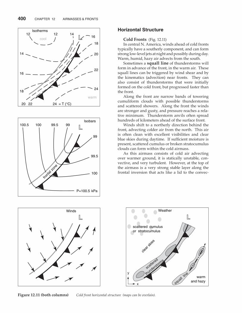
horizontal structure
Cold Fronts (Fig. 12.11) In central N. America, winds ahead of cold fronts typically have a southerly component, and can form strong low-level jets at night and possibly during day. Warm, humid, hazy air advects from the south. Sometimes a squall line of thunderstorms will form in advance of the front, in the warm air. These squall lines can be triggered by wind shear and by the kinematics (advection) near fronts. They can also consist of thunderstorms that were initially formed on the cold front, but progressed faster than the front. Along the front are narrow bands of towering cumuliform clouds with possible thunderstorms and scattered showers. Along the front the winds are stronger and gusty, and pressure reaches a rela-tive minimum. Thunderstorm anvils often spread hundreds of kilometers ahead of the surface front. Winds shift to a northerly direction behind the front, advecting colder air from the north. This air is often clean with excellent visibilities and clear blue skies during daytime. If sufficient moisture is present, scattered cumulus or broken stratocumulus clouds can form within the cold airmass. As this airmass consists of cold air advecting over warmer ground, it is statically unstable, con-vective, and very turbulent. However, at the top of the airmass is a very strong stable layer along the frontal inversion that acts like a lid to the convec-
Figure 12.11 (both columns) Cold front horizontal structure (maps can be overlain).
r. STULL • METEOrOLOGy FOr SCiENTiSTS AND ENGiNEErS 401
tion. Sometimes over ocean surfaces the warm moist ocean leads to considerable post-frontal deep convection. The idealized picture presented in Fig. 12.11 can differ considerably in the mountains.
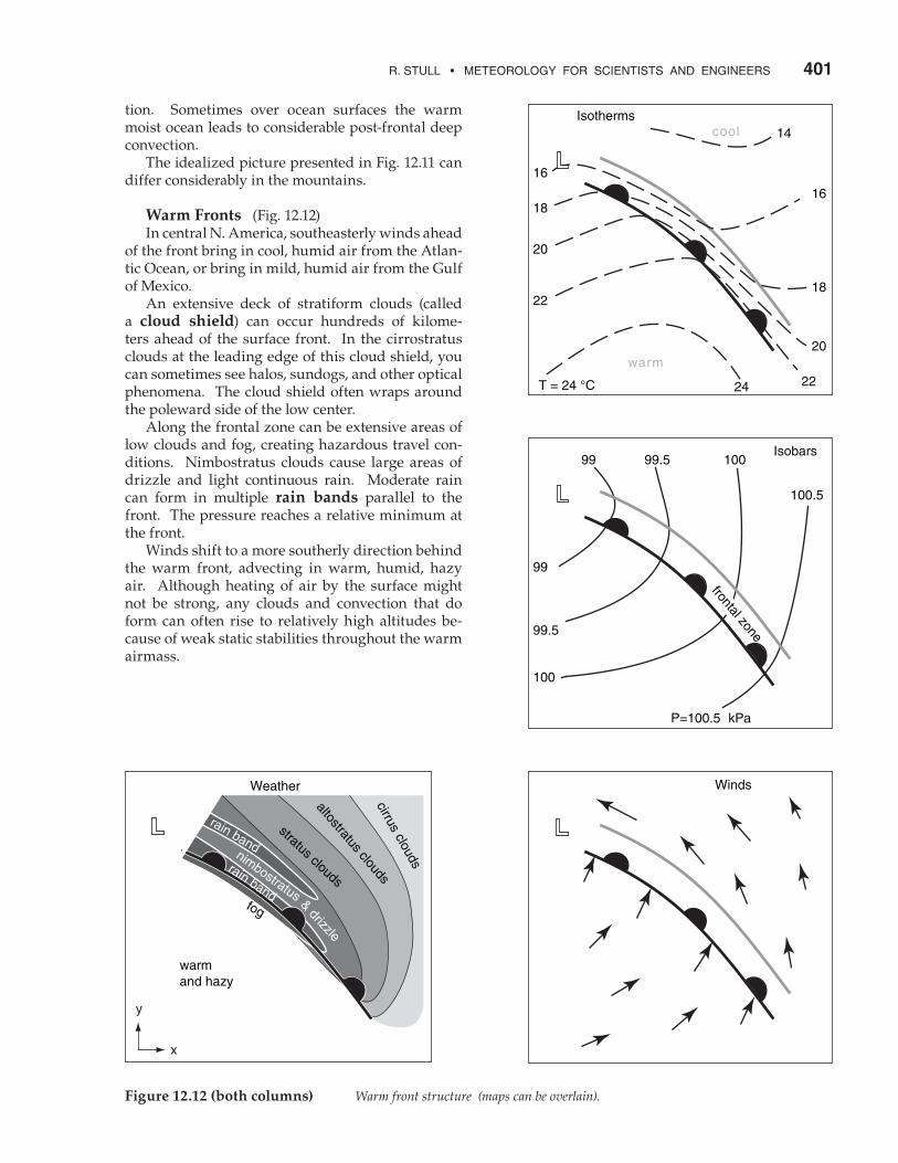
Warm Fronts (Fig. 12.12) In central N. America, southeasterly winds ahead of the front bring in cool, humid air from the Atlan-tic Ocean, or bring in mild, humid air from the Gulf of Mexico. An extensive deck of stratiform clouds (called a cloud shield) can occur hundreds of kilome-ters ahead of the surface front. In the cirrostratus clouds at the leading edge of this cloud shield, you can sometimes see halos, sundogs, and other optical phenomena. The cloud shield often wraps around the poleward side of the low center. Along the frontal zone can be extensive areas of low clouds and fog, creating hazardous travel con-ditions. Nimbostratus clouds cause large areas of drizzle and light continuous rain. Moderate rain can form in multiple rain bands parallel to the front. The pressure reaches a relative minimum at the front. Winds shift to a more southerly direction behind the warm front, advecting in warm, humid, hazy air. Although heating of air by the surface might not be strong, any clouds and convection that do form can often rise to relatively high altitudes be-cause of weak static stabilities throughout the warm airmass.
Figure 12.12 (both columns) Warm front structure (maps can be overlain).
402 CHAPTEr 12 AirMASSES & FrONTS
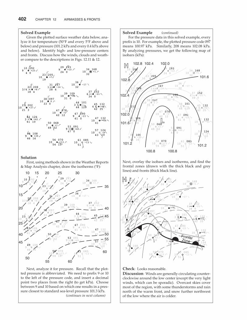
Solved Example Given the plotted surface weather data below, ana-lyze it for temperature (50°F and every 5°F above and below) and pressure (101.2 kPa and every 0.4 kPa above and below). Identify high- and low-pressure centers and fronts. Discuss how the winds, clouds and weath-er compare to the descriptions in Figs. 12.11 & 12.
Solution First, using methods shown in the Weather Reports & Map Analysis chapter, draw the isotherms (°F):
Next, analyze it for pressure. Recall that the plot-ted pressure is abbreviated. We need to prefix 9 or 10 to the left of the pressure code, and insert a decimal point two places from the right (to get kPa). Choose between 9 and 10 based on which one results in a pres-sure closest to standard sea-level pressure 101.3 kPa. (continues in next column)
Solved Example (continued) For the pressure data in this solved example, every prefix is 10. For example, the plotted pressure code 097 means 100.97 kPa. Similarly, 208 means 102.08 kPa. By analyzing pressures, we get the following map of isobars (kPa):
Next, overlay the isobars and isotherms, and find the frontal zones (drawn with the thick black and grey lines) and fronts (thick black line).
Check: Looks reasonable.Discussion: Winds are generally circulating counter-clockwise around the low center (except the very light winds, which can be sporadic). Overcast skies cover most of the region, with some thunderstorms and rain north of the warm front, and snow further northwest of the low where the air is colder.
9
10
57 124−9
4310
61 085−13
5110
56 070+13
54 1510
47 090−23
41 09
47 132−14
4110
53 091+40
47 09
50 068+1
48 327
49 108+39
46 169
43 126+42
41 103
45 132−9
42 354
37 152−21
34 06
44 101
44 1293
47 078−5
42 1210
39 109−26
31 010
36−17
3210
23 202+37
21 310
38 0970
33 010
34 168+1
3210
31 147−14
28 61
23 205+7
1910
22 208+8
18 43/4
29 193+10
24 0910 292
+104 0

r. STULL • METEOrOLOGy FOr SCiENTiSTS AND ENGiNEErS 403
Vertical structure Suppose that radiosonde observations (RAOBs) are used to probe the lower troposphere, providing temperature profiles such as those in Fig. 12.13a. To locate fronts by their vertical cross section, first con-vert the temperatures into potential temperatures θ (Fig. 12.13b). Then, draw lines of equal potential tem-perature (isentropes). Fig. 12.13c shows isentropes drawn at 5°C intervals. Often isentropes are labeled in Kelvin. In the absence of diabatic processes such as latent heating, radiative heating, or turbulent mixing, air parcels follow isentropes when they move adiabati-cally. For example, consider the θ = 35°C parcel that is circled in Fig. 12.13b above weather station B. Sup-pose this parcel starts to move westward toward C. If the parcel were to be either below or above the 35°C isentrope at its new location above point C, buoyant forces would tend to move it vertically to the 35°C isentrope. Such forces happen continuous-ly while the parcel moves, constantly adjusting the altitude of the parcel so it rides on the isentrope. The net movement is westward and upward along the 35°C isentrope. Air parcels that are forced to rise along isentropic surfaces can form clouds and precipitation, given sufficient moisture. Similarly, air blowing eastward would move downward along the sloping isentrope. In three dimensions, you can picture isentropic surfaces separating warmer θ aloft from colder θ below. Analysis of the flow along these surfaces provides a clue to the weather associated with the front. Air parcels moving adiabatically must follow the “topography” of the isentropic surface. This is illustrated in the Extratropical Cyclones chapter. At the Earth’s surface, the boundary between cold and warm air is the surface frontal zone. This is the region where isentropes are packed rela-tively close together (Figs. 12.13b & c). The top of the cold air is called the frontal inversion (Fig. 12.13c). The frontal inversion is also evident at weather sta-tions C and D in Fig. 12.13a, where the temperature increases with height. Frontal inversions of warm and cold fronts are gentle and of similar tempera-ture change. Within about 200 m of the surface, there are ap-preciable differences in frontal slope. The cold front has a steeper nose (slope ≈ 1 : 100) than the warm front (slope ≈ 1 : 300), although wide ranges of slopes have been observed. Fronts are defined by their temperature struc-ture, although many other quantities change across the front. Advancing cold air at the surface defines
Solved Example What weather would you expect with a warm katafront? (See next page.)
Solution & Discussion Cumuliform clouds and showery precipitation would probably be similar to those in Fig. 12.16a, ex-cept that the bad weather would move in the direction of the warm air at the surface, which is the direction the surface front is moving.
Figure 12.13Analysis of soundings to locate fronts in a vertical cross section. Frontal zone / frontal inversion is shaded in bottom figure, and is located where the isentropes are tightly packed (close to each other).

404 CHAPTEr 12 AirMASSES & FrONTS
the cold front, where the front moves toward the warm airmass (Fig. 12.14a). Retreating cold air de-fines the warm front, where the front moves to-ward the cold airmass (Fig. 12.14b). Above the frontal inversion, if the warm air flows down the frontal surface, it is called a katafront, while warm air flowing up the frontal surface is an anafront (Fig. 12.15). It is possible to have cold katafronts, cold anafronts, warm katafronts, and warm anafronts. Frequently in central N. America, the cold fronts are katafronts, as sketched in Fig. 12.16a. For this sit-uation, warm air is converging on both sides of the frontal zone, forcing the narrow band of cumuliform clouds that is typical along the front. It is also com-mon that warm fronts are anafronts, which leads to a wide region of stratiform clouds caused by the warm air advecting up the isentropic surfaces (Fig. 12.16b). A stationary front is like an anafront where the cold air neither advances nor retreats.
geostrophiC aDjUstMent – part 3
Winds in the Cold air Why does cold dense air from the poles not spread out over more of the Earth, like a puddle of water? Coriolis force is the culprit, as shown next. Picture two air masses initially adjacent (Fig. 12.17a). The cold airmass has initial depth H and uniform virtual potential temperature θv1. The warm airmass has uniform virtual potential tem-perature θv1 + ∆θv. The average absolute virtual temperature is Tv . In the absence of rotation of the coordinate system, you would expect the cold air to spread out completely under the warm air due to buoyancy, reaching a final state that is horizontally homogeneous. However, on a rotating Earth, the cold air expe-riences Coriolis force (to the right in the Northern Hemisphere) as it begins to move southward. In-stead of flowing across the whole surface, the cold air spills only distance a before the winds have turned 90°, at which point further spreading stops (Fig. 12.17b). At this quasi-equilibrium, pressure-gradient force associated with the sloping cold-air interface balances Coriolis force, and there is a steady geo-strophic wind Ug from east to west. The process of approaching this equilibrium is called geostrophic adjustment, as was discussed in the previous chap-ter. Real atmospheres never quite reach this equi-librium.
Figure 12.14Vertical structure of fronts, based on cold air movement.
Figure 12.15Vertical structure of fronts, based on overlying-air movement.
Figure 12.16Typical fronts in central N. America.

r. STULL • METEOrOLOGy FOr SCiENTiSTS AND ENGiNEErS 405
At equilibrium, the final spillage distance a of the front from its starting location equals the exter-nal Rossby-radius of deformation, λR:
ag H T
fRv v
c= =
∆λ
θ· · / •(12.5)
where fc is the Coriolis parameter and |g| = 9.8 m/s2 is gravitational acceleration magnitude. The geostrophic wind Ug in the cold air at the surface is greatest at the front (neglecting friction), and exponentially decreases behind the front:
U g H Ty a
ag v v= − −+
· ·( / ) ·exp∆θ •(12.6)
for –a ≤ y ≤ ∞ . The depth of the cold air h is:
h Hy a
a= − −
+
· exp1 •(12.7)
which smoothly increases to depth H well behind the front (at large y). Figs. 12.17 are highly idealized, having airmasses of distinctly different temperatures with a sharp in-terface in between. For a fluid with a smooth contin-uous temperature gradient, geostrophic adjustment occurs in a similar fashion, with a final equilibrium state as sketched in Fig. 12.18. The top of this dia-gram represents the top of the troposphere, and the top wind vector represents the jet stream. This state has high surface pressure under the cold air, and low surface pressure under the warm air (see the Global Circulation chapter). On the cold side, isobaric surfaces are more-closely spaced in height than on the warm side, due to the hypsometric relationship. This results in a pressure reversal aloft, with low pressure (or low heights) above the cold air and high pressure (or high heights) above the warm air. Horizontal pressure gradients at low and high altitudes create opposite geostrophic winds, as in-dicated in Fig. 12.18. Due to Coriolis force, the air represented in Fig. 12.18 is in equilibrium; namely, the cold air does not spread any further. This behavior of the cold airmass is extremely significant. It means that the planetary-scale flow, which is in approximate geostrophic balance, is un-able to complete the job of redistributing the cold air from the poles and warm air from the tropics. Yet some other process must be acting to complete the job of redistributing heat to satisfy the global energy budget (in the Global Circulation chapter).
Figure 12.17Geostrophic adjustment of a cold front. (a) Initial state. (b) Final state is in dynamic equilibrium, which is never quite at-tained in the real atmosphere.
Figure 12.18Final dynamic state after geostrophic adjustment within an envi-ronment containing continuous temperature gradients. Arrows represent geostrophic wind. Shaded areas are isobaric surfaces. H and L indicate high and low pressures relative to surrounding pressures at the same altitude. Dot-circle represents the tip of an arrow pointing toward the reader, x-circle represents the tail feathers of an arrow pointing into the page.

406 CHAPTEr 12 AirMASSES & FrONTS
That other process is the action of cyclones and Rossby waves. Many small-scale, short-lived cy-clones are not in geostrophic balance, and they can act to move the cold air further south, and the warm air further north. These cyclones feed off the poten-tial energy remaining in the large-scale flow, namely, the energy associated with horizontal temperature gradients. Such gradients have potential energy that can be released when the colder air slides under the warmer air (see Fig. 11.1).
BeyonD algeBra • geostrophic adjust-ment
We can verify that the near-surface (friction-less) geostrophic wind is consistent with the sloping depth of cold air. The geostrophic wind is related to the horizontal pressure gradient at the surface by:
Uf
Pyg
c= − 1
ρ··∆∆
(10.26a)
Assume that the pressure at the top of the cold air-mass in Figs. 12.17 equals the pressure at the same altitude h in the warm airmass. Thus, surface pres-sures will be different due to only the difference in weight of air below that height. Going from the top of the sloping cold airmass to the bottom, the vertical increase of pressure is given by the hydrostatic eq: ∆P g hcold cold= −ρ · ·A similar equation can be written for the warm air below h. Thus, at the surface, the difference in pres-sures under the cold and warm air masses is: ∆P g h cold warm= − −· ·( )ρ ρmultiplying the RHS by ρ / ρ , where ρ is an aver-age density, yields: ∆P g h cold warm= − −· · ·[( )/ ]ρ ρ ρ ρAs was shown in the Buoyancy section of the Stability chapter, use the ideal gas law to convert from density to virtual temperature, remembering to change the sign because the warmer air is less dense. Also, ∆Tv = ∆θv. Thus: ∆P g h Tv warm v cold v= − −· · ·[( )/ ]ρ θ θwhere this is the pressure change in the negative y direction. Plugging this into eq. (10.26a) gives:
Ug T
fhyg
v v
c= −
·( / )·
∆ ∆∆
θ
which we can write in differential form:
Ug T
fhyg
v v
c= − ∂
∂·( / )
·∆θ
(b)
The equilibrium value of h was given by eq. (12.7): h H
y aa
= − −+
· exp1 (12.7)Thus, the derivative is:
∂∂
= −+
hy
Ha
y aa
·exp
Plugging this into eq. (b) gives:
Ug T
fHa
y aag
v v
c= − −
+
·( / )· ·exp
∆θ (c)
But from eq. (12.5) we see that: f a f g H Tc c R v v· · · ·( / )= =λ θ∆ (12.5)
Eq. (c) then becomes:
U g H Ty a
ag v v= − −+
· ·( / ) ·exp∆θ (12.6)
Thus, the wind is consistent (i.e., geostrophically bal-anced) with the sloping height.
Solved Example A cold airmass of depth 1 km and virtual potential temperature 0°C is imbedded in warm air of virtual potential temperature 20°C. Find the Rossby deforma-tion radius, the maximum geostrophic wind speed, and the equilibrium depth of the cold airmass at y = 0. Assume fc = 10–4 s–1 .
SolutionGiven: Tv = 280 K, ∆θv = 20 K, H = 1 km, fc = 10–4 s–1 .Find: a = ? km, Ug = ? m/s at y = –a, and h = ? km at y = 0.
Use eq. (12.5):
a =−
− −( . · )·( )·( )/( )9 8 1000 20 280
10 4m s m K K
s
2
1
= 265 km
Use eq. (12.6): Ug = − ( )−( . · )( )( )/( ) ·exp9 8 1000 20 280 0m s m K K2
= –26.5 m/s
Use eq. (12.7):
h = − −( )[ ]( )· exp1 1 1km = 0.63 km
Check: Units OK. Physics OK.Discussion: Frontal-zone widths on the order of a = 200 km are small compared to lengths (1000s km).

r. STULL • METEOrOLOGy FOr SCiENTiSTS AND ENGiNEErS 407
Winds in the Warm over-riding air Across the frontal zone is a stronger-than-back-ground horizontal temperature gradient. In many fronts, the horizontal temperature gradient is stron-gest near the surface, and weakens with increasing altitude. The thermal-wind relationship tells us that the geostrophic wind will increase with height in strong horizontal temperature gradients. If the frontal zone extends vertically over a large portion of the troposphere, then the wind speed will continue to increase with height, reaching a maximum near the tropopause. Thus, jet streams are associated with frontal zones. The jet blows parallel to the frontal zone, with greatest wind speeds on the warm side of the frontal zone. If the cold air is advancing as a cold front, then this jet is known as a pre-frontal jet. This is illustrated in Fig. 12.19. Plotted are isentropes, isobars, isotachs, and the frontal zone. The cross-frontal direction is north-south in this fig-ure, causing a pre-frontal jet from the West (blowing into the page, in this diagram).
Frontal Vorticity Combining the cold-air-side winds from Fig. 12.17b and warm-air-side winds from Fig. 12.19 into a single diagram yields Fig. 12.20. In this sketch, the warm air aloft and south of the front has geostroph-ic winds from the west, while the cold air near the ground has geostrophic winds from the east. Thus, across the front, ∆Ug/∆y is negative, which means that the relative vorticity (eq. 11.20) of the geostrophic wind is positive (ζr = +) at the front (grey curved arrows in Fig. 12.20). In fact, cyclonic vorticity is found along fronts of any orientation. Also, stronger density contrasts across fronts cause greater positive vorticity. Also, frontogenesis (strengthening of a front) is often associated with horizontal convergence of air from opposite sides of the front (see next section). Horizontal convergence implies vertical divergence (i.e., vertical stretching of air and updrafts) along the front, as required by mass continuity. But stretch-ing increases vorticity (see the chapters on Stabil-ity, Global Circulation, and Extratropical Cyclones). Thus, frontogenesis is associated with updrafts (and associated clouds and bad weather) and with in-creasing relative vorticity.
Figure 12.19Vertical section across a cold front in the N. Hemisphere. Thick lines outline the frontal zone in the troposphere, and show the tropopause in the top of the graph. Medium black lines are isobars. Thin grey lines are isentropes. Shaded areas indicate isotachs, for a jet that blows from the West (into the page).
Figure 12.20Sketch of cold front, combining winds in the cold air (thick straight grey arrow) from Fig. 12.17b with the winds in the warm air (thick white arrow) from Fig. 12.19. These winds cause shear across the front, shown with the black arrows. This shear is associated with positive (cyclonic) relative vorticity of the geostrophic wind (thin curved grey arrows).

408 CHAPTEr 12 AirMASSES & FrONTS
Frontogenesis
Fronts are recognized by the change in tempera-ture across the frontal zone — greatest at the sur-face. Hence, the horizontal temperature gradient (temperature change per distance across the front) is one measure of frontal strength. Usually potential temperature is used instead of temperature to sim-plify the problem when vertical motions can occur. Physical processes that tend to increase the po-tential-temperature gradient are called frontoge-netic — literally they cause the birth or strengthen-ing of the front. Three classes of such processes are kinematic, thermodynamic, and dynamic.
Kinematics Kinematics refers to motion or advection, with no regard for driving forces. This class of processes cannot create potential-temperature gradients, but it can strengthen or weaken existing gradients. From earlier chapters, we saw that radiative heating causes north-south temperature gradients between the equator and poles. Also, the general circulation causes the jet stream to meander, which creates transient east-west temperature gradients along troughs and ridges. The standard-atmosphere also has a vertical gradient of potential temperature in the troposphere (θ increases with z). Thus, it is fair to assume that temperature gradients often ex-ist, which could be strengthened during kinematic frontogenesis. To illustrate kinematic frontogenesis, consider an initial potential-temperature field with uniform gradients in the x, y, and z directions, as sketched in Fig. 12.21. The gradients have the following signs (for this particular example):
∆∆
= +θx
∆∆
= −θy
∆∆
= +θz
(12.8)
Namely, potential temperature increases toward the east, decreases toward the north, and increases up-ward. There are no fronts in this picture initially. We will examine the subset of advections that tends to create a cold front aligned north-south. De-fine the strength of the front as the potential-tem-perature gradient across the front:
Frontal Strength = FSx
= ∆∆
θ •(12.9)
The change of frontal strength with time due to advection is given by the kinematic frontogenesis equation:
FoCUs • the polar Front
Because of Coriolis force, cold arctic air cannot spread far from the poles, causing a quasi-permanent frontal boundary in the winter hemisphere. This is called the polar front. It has a wavy irregular shape where some seg-ments advance as cold fronts, other segments retreat as warm fronts, some are stationary, and others are weak and cause gaps in the front.
Figure a. Top: Vertical slice through the North Pole. Bottom: View from space looking down on N. Pole.
Figure 12.21Vertical and horizontal slices through a volume of atmosphere, showing initial conditions prior to frontogenesis. The thin hori-zontal dashed lines show where the planes intersect.

r. STULL • METEOrOLOGy FOr SCiENTiSTS AND ENGiNEErS 409
•(12.10)
∆
∆= − ∆
∆
∆∆
− ∆
∆
∆( )· ·
FSt x
Ux y
θ θ VVx z
Wx∆
− ∆
∆
∆∆
θ·
Strengthening Confluence Shear Tilting
Confluence Suppose there is a strong west wind U approach-ing from the west, but a weaker west wind depart-ing at the east (Fig. 12.22 top). Namely, the air from the west almost catches up to air in the east. For this situation, ∆U/∆x = – , and ∆θ/∆x = + in eq. (12.10). Hence, the product of these two terms, when multiplied by the negative sign attached to the confluence term, tends to strengthen the front [∆(FS)/∆t = + ]. In the shaded region of Fig. 12.22, the isentropes are packed closer together; namely, it has become a frontal zone.
Shear Suppose the wind from the south is stronger on the east side of the domain than the west (Fig. 12.23 top). This is one type of wind shear. As the isentropes on the east advect northward faster than those on the west, the potential-temperature gradi-ent is strengthened in-between, creating a frontal zone. While the shear is positive (∆V/∆x = +), the north-ward temperature gradient is negative (∆θ/∆y = – ). Thus, the product is positive when the preceding negative sign from the shear term is included. Fron-tal strengthening occurs for this case [∆(FS)/∆t = + ].
Tilting If updrafts are stronger on the cold side of the domain than the warm side, then the vertical po-tential-temperature gradient will be tilted into the horizontal. The result is a strengthened frontal zone (Fig. 12.24). The horizontal gradient of updraft velocity is negative in this example (∆W/∆x = – ), while the vertical potential-temperature gradient is positive (∆θ/∆z = + ). The product, when multiplied by the negative sign attached to the tilting term, yields a positive contribution to the strengthening of the front for this case [∆(FS)/∆t = + ]. While this example was contrived to illustrate frontal strengthening, for most real fronts, the tilt-ing term causes weakening. Such frontolysis is weakest near the surface because vertical motions are smaller there (the wind cannot blow through the ground). Tilting is important and sometimes dominant for upper-level fronts, as described later.
Figure 12.22Confluence strengthens the frontal zone (shaded) in this case. Arrow tails indicate starting locations for the isotherms.
Figure 12.23Shear strengthens the frontal zone (shaded) in this case. Arrow tails indicate starting locations for the isotherms.
Figure 12.24Tilting of the vertical temperature gradient into the horizontal strengthens the frontal zone (shaded) in this illustration.

410 CHAPTEr 12 AirMASSES & FrONTS
Deformation The previous figures presented idealized kine-matic scenarios. Often in real fronts the flow field is a more complex combination of scenarios. For ex-ample, Fig. 12.25 shows a deformation (change of shape) flow field in the cold air, with confluence ( → ← coming together horizontally) of air perpen-dicular to the front, and diffluence ( ← → hori-zontal spreading of air) parallel to the front. In such a flow field both convergence and shear affect the temperature gradient. For example, con-sider the two identical deformation fields in Figs. 12.26a & b, where the only difference is the angle of the isentropes in a frontal zone relative to the axis of dilation (the line toward which confluence points, and along which diffluence spreads). For initial angles less than 45° (Fig. 12.26a & a’), the isentropes are pushed closer together (frontogenesis) and tilted toward a shallower angle. For initial angles greater than 45°, the isentropes are spread farther apart (frontolysis) and tilted toward a shallower angle. Using this info to analyze Fig. 12.25 where the isentropes are more-or-less paral-lel to the frontal zone (i.e., initial angle << 45°), we would expect that flow field to cause frontogenesis.
Solved Example Given an initial environment with ∆θ/∆x = 0.01°C/km, ∆θ/∆y = –0.01°C/km, and ∆θ/∆z = 3.3°C/km. Also, suppose that ∆U/∆x = – 0.05 (m/s)/km, ∆V/∆x = 0.05 (m/s)/km, and ∆W/∆x = 0.02 (cm/s)/km. Find the kinematic frontogenesis rate.
SolutionGiven: (see above)Find: ∆(FS)/∆t = ? °C·km–1·day–1
Use eq. (12.10):
∆∆
= −
−
− −( )
. · .FSt
0 01 0 05 0°Ckm
m/skm
.. ·
. .
01
0 05 3 3
°
°
Ckm
m/skm
Ckm
−
· .0 0002
m/skm
= +0.0005 + 0.0005 – 0.00066 °C·m·s–1·km–2 = +0.029 °C·km–1·day–1
Check. Units OK. Physics OK.Discussion: Frontal strength ∆θ/∆x nearly tripled in one day, increasing from 0.01 to 0.029 °C/km.
Figure 12.25An illustration of the near-surface horizontal air-flow pattern at a frontal zone.
Figure 12.26Black arrows are wind, and grey arrows are isentropes. Dashed line is the axis of dilation. (a) and (a’) are initial and final states for shallow initial angle, showing frontogenesis. The shaded area in (a’) highlights the strengthened frontal zone. (b) and (b’) are initial and final states for steep initial angle, showing front-olysis. (after J. Martin, 2006: “Mid-Latitude Atmospheric Dy-namics: A First Course. Wiley.)

r. STULL • METEOrOLOGy FOr SCiENTiSTS AND ENGiNEErS 411
thermodynamics The previous kinematic examples showed adia-batic advection (potential temperature was con-served while being blown with the wind). However, diabatic (non-adiabatic) thermodynamic processes can heat or cool the air at different rates on either side of the domain. These processes include radia-tive heating/cooling, conduction from the surface, turbulent mixing across the front, and latent heat re-lease/absorption associated with phase changes of water in clouds. Define the diabatic warming rate (DW) as:
Diabatic Warming Rate = =DWt
∆∆θ •(12.11)
If diabatic heating is greater on the warm side of the front than the cold side, then the front will be strengthened:
∆
∆= ∆
∆( ) ( )FS
tDW
x •(12.12)
In most real fronts, turbulent mixing between the warm and cold sides weakens the front (i.e., causes frontolysis). Conduction from the surface also contributes to frontolysis. For example, behind a cold front, the cold air blows over a usually-warm-er surface, which heats the cold air (i.e., airmass modification) and reduces the temperature contrast across the front. Similarly, behind warm fronts, the warm air is usually advecting over cooler surfaces. Over both warm and cold fronts, the warm air is often forced to rise. This rising air can cause con-densation and cloud formation, which strengthen fronts by warming the already-warm air. Radiative cooling from the tops of stratus clouds reduces the temperature on the warm side of the front, contributing to frontolysis of warm fronts. Radiative cooling from the tops of post-cold frontal stratocumulus clouds can strengthen the front by cooling the already-cold air.
Dynamics Kinematics and thermodynamics are insufficient to explain observed frontogenesis. While kinematic frontogenesis gives doubling or tripling of frontal strength in a day (see previous solved examples), observations show that frontal strength can increase by a factor of 15 during a day. Dynamics can cause this rapid strengthening. Because fronts are long and narrow, we expect along-front flow to tend toward geostrophy, while across front flows could be ageostrophic. We can an-ticipate this by using the Rossby number (see Fo-
Solved Example A thunderstorm on the warm side of a 200 km wide front rains at 2 mm/h. Find the frontogenesis rate.
SolutionGiven: RR = 0 at x = 0, and RR = 2 mm/h at x = 200 kmFind: ∆(FS)/∆t = ? °C·km–1·day–1
From the Heat chapter: ∆θ/∆t = (0.33°C/mm)·RR = 0.66°C/h.
Combine eqs. (12.11) & (12.12): ∆(FS)/∆t = ∆(∆θ/∆t)/∆x
∆(FS)/∆t = [(0.66°C/h)·(24 h/day) – 0] / [200 km – 0] = (15.84°C/day)/(200km) = 0.079 °C·km–1·day–1
Check: Units OK. Physics OK. Magnitude good.Discussion: This positive value indicates thermody-namic frontogenesis.
Figure 12.27Isobaric surfaces near a hypothetical front, before being altered by dynamics. Vectors show equilibrium geostrophic winds, ini-tially (state “o”). Dot-circle (1) represents the tip of an arrow pointing toward the reader; x-circle (2) represents the tail feath-ers of an arrow pointing into the page.

412 CHAPTEr 12 AirMASSES & FrONTS
cus Box in the Dynamics chapter). Fronts can be of order 1000 km long, but of order 100 km wide. Thus, the Rossby number for along-front flow is of order Ro = 0.1 . But the across-front Rossby number is of order Ro = 1. Recall that flows tend toward geostro-phy when Ro < 1. Thus, ageostrophic dynamics are anticipated across the front, as are illustrated next. Picture an initial state in geostrophic equilibrium with winds parallel to the front, as sketched in Fig. 12.27. This figure shows a special situation where pressure gradients and geostrophic winds exist only midway between the left and right sides. Zero gra-dients and winds are at the left and right sides. A frontal zone is in the center of this diagram. Suppose some external forcing such as kinematic confluence due to a passing Rossby wave causes the front to strengthen a small amount, as sketched in Fig. 12.28a. Not only does the potential-temperature gradient tighten, but the pressure gradient also in-creases due to the hypsometric relationship. The increased pressure gradient implies a differ-ent, increased geostrophic wind. However, initial-ly, the actual winds are slower due to inertia, with magnitude equal to the original geostrophic speed. While the actual winds adjust toward the new geostrophic value, they temporarily turn away from the geostrophic direction (Fig. 12.29) due to the im-balance between pressure-gradient and Coriolis forces. During this transient state (b), there is a component of wind in the x-direction (Fig. 12.28b). This is called ageostrophic flow, because there is no geostrophic wind in the x-direction. Because mass is conserved, horizontal conver-gence and divergence of the U-component of wind cause vertical circulations. These are thermally di-rect circulations, with cold air sinking and warm air rising and moving over the colder air. The result is a temporary cross-frontal, or transverse circula-tion called a Sawyer-Eliassen circulation. The updraft portion of the circulation can drive convec-tion, and cause precipitation. The winds finally reach their new equilibrium value equal to the geostrophic wind. In this final state, there are no ageostrophic winds, and no cross-frontal circulation. However, during the preceding transient stage, the ageostrophic cross-frontal cir-culation caused extra dynamic confluence near the surface, which adds to the original kinematic con-fluence to strengthen the surface front. The trans-verse circulation also tilts the front (Fig. 12.28c). In summary, a large and relatively steady geo-strophic wind blows parallel to the front (Fig. 12.27). A weak, transient, cross-frontal circulation can be superimposed (Fig. 12.28b). These two factors are also important for upper-tropospheric fronts, as de-scribed later.
Figure 12.29Time lines labeled 1 & 2 are for the vectors 1 & 2 in Fig. 12.27. Initial state (o) is given by Fig. 12.27. Later states (a)-(c) corre-spond to Figs. 12.28(a)-(c). The ageostrophic wind (ag) at time (b) is also indicated. States (o) and (c) are balanced.
Figure 12.28Vertical cross section showing dynamic strengthening of a front. The frontal zone is shaded; lines are isobars; and arrows are ageostrophic winds. D and C are regions of horizontal di-vergence and convergence. (a) Initial state (thin dashed lines) modified (thick lines) by confluence (arrows). (b) Ageostrophic circulation, called a Sawyer-Eliassen circulation. (c) Final equi-librium state.

r. STULL • METEOrOLOGy FOr SCiENTiSTS AND ENGiNEErS 413
oCClUDeD Fronts anD MiD-
tropospheriC Fronts
When three or more airmasses come together, such as in an occluded front, it is possible for one or more fronts to ride over the top of a colder airmass. This creates lower- or mid-tropospheric fronts that do not touch the surface, and which would not be signaled by temperature changes and wind shifts at the surface. However, such fronts aloft can trigger clouds and precipitation observed at the surface. Occluded fronts occur when cold fronts catch up to warm fronts. What happens depends on the temperature and static-stability difference between
the cold advancing air behind the cold front and the cold retreating air ahead of the warm front. Fig. 12.30 shows a cold front occlusion, where very cold air that is very statically stable catches up to, and under-rides, cooler air that is less statically stable. The warm air that was initially between these two cold airmasses is forced aloft. Most oc-clusions in interior N. America are of this type, due to the very cold air that advances from Canada in winter. Observers at the surface would notice stratiform clouds in advance of the front, which would nor-mally signal an approaching warm front. However, instead of a surface warm front, a surface occluded front passes, and the surface temperature decreases like a cold front. The trailing edge of cool air aloft marks the warm front aloft.
Figure 12.30Cold front occlusion. (a) Surface map showing position of sur-face cold front (dark triangles), surface warm front (dark semi-circles), surface occluded front (dark triangles and semicircles), and warm front aloft (white semicircles). (b) Vertical cross sec-tion along slice A-B from top diagram. Diagonal lines = rain.
Figure 12.31Warm front occlusion. (a) Surface map. Symbols are similar to Fig. 12.30, except that white triangles denote a cold front aloft. (b) Vertical cross section along slice C-D from top diagram. TROWAL = trough of warm air aloft. The open grey circle shows the triple-point location (meeting of 3 surface fronts).

414 CHAPTEr 12 AirMASSES & FrONTS
The location in Figs. 12.30 and 12.31 where the cold, warm, and occluded fronts intersect at the sur-face is called the triple point. Fig. 12.31 shows a warm front occlusion, where cool air that is less statically stable catches up to, and over-rides, colder air that is more stati-cally stable, forcing aloft the warm air that was in-between. Most occlusions in Europe and the Pacific Northwest USA are this type, due to mild cool air that advances from over the cool ocean during win-ter. Observers at the surface notice stratiform clouds in advance of the front. But before the surface front arrives, there can be showers or thunderstorms as-sociated with the cool front aloft. Later, a surface occluded front passes with widespread drizzle, and the surface temperature warms. Fig. 12.32 shows how the static stability relates to the type of occlusion. In this sketch of a warm front occlusion, look at the static stability across the oc-cluded front, at the altitude of the dashed line. To the east of the front in the cold airmass, the air is strongly stable (as shown by the tight packing of the isentropes in the vertical). To the west in the cool airmass, the air is less statically stable (i.e., greater vertical spacing between isentropes). If this had been a cold frontal occlusion instead, the greatest static stability would have been west of the front. The wedge of warm air (Fig. 12.32) pushed up between the cool and cold airmasses is called a TROWAL, an acronym that means “trough of warm air aloft.” This TROWAL, labeled in Fig. 12.31a, touches the ground at the triple point, but tilts toward higher altitudes further north. Under the TROWAL can be significant precipitation and se-vere weather at the surface (Fig. 12.31b) — hence it is important for weather forecasting. The previous sketches are “text-book” examples of prototypical situations. In real life, more complex maps and cross sections can occur. Sometimes more than three airmasses can be drawn together in a low, causing multiple cold or warm fronts, and multiple fronts aloft.
Upper-tropospheriC Fronts
Upper-tropospheric fronts are also called upper-level fronts, and are sometimes associated with folds in the tropopause. A cross-section through an idealized upper-level front is sketched in Fig. 12.33. In the lower troposphere, the south-to-north tem-perature gradient creates the jet stream due to the thermal wind relationship (see the Global Circula-
Figure 12.32Idealized vertical cross-section through a warm front occlusion, showing the bottom 5 km of the troposphere. Dark grey lines are isentropes. Light grey shading indicates strong static stability (regions where the isentropes are packed closer together in the vertical). TROWAL = trough of warm air aloft.
Figure 12.33Idealized vertical cross-section through the jet stream in N. Hemisphere. Shading indicates west-to-east speeds (into the page): light ≥ 50 m/s, medium ≥ 75 m/s, dark ≥ 100 m/s. Thin lines are isentropes (K). Thick line is the tropopause. “Front” indicates the upper-tropospheric front, where stratospheric air is penetrating into the troposphere.

r. STULL • METEOrOLOGy FOr SCiENTiSTS AND ENGiNEErS 415
tion chapter). A reversal of the meridional tempera-ture gradient above 10 km in this idealized sketch causes wind velocities to decrease above that alti-tude. Within the stratosphere, the isentropes are spaced closer together, indicating greater static sta-bility. South of the core of the jet stream, the tropopause is relatively high. To the north, it is lower. Between these two extremes, the tropopause can wrap around the jet core, and fold back under the jet, as sketched in Fig. 12.33. Within this fold the isentropes are tightly packed, indicating an upper-tropospheric front. Sometimes the upper-level front connects with a surface front (Fig. 12.19). Stratospheric air has unique characteristics that allow it to be traced. Relative to the troposphere, stratospheric air has high ozone content, high radio-activity (due to former nuclear bomb testing), high static stability, low water-vapor mixing ratio, and high isentropic potential vorticity. The tropopause fold brings air of stratospheric origin down into the troposphere. This causes an injection of ozone and radioactivity into the tropo-sphere. The dry air in the tropopause fold behind the cold front is often clearly visible in water-vapor satellite images of the upper troposphere. The heavy line in Fig. 12.33 corresponds roughly to the 1.5 PVU (potential vorticity units) isopleth, and is a good indicator of the tropopause. Above this line, PVU values are greater than 1.5, and in-crease rapidly with height to values of roughly 10 PVU at the top of Fig. 12.33. Below this line, the PVU gradient is weak, with typical values of about 0.5 PVU at mid-latitudes. PVU is negative in the South-ern Hemisphere, but of similar magnitude. Sawyer-Eliassen dynamics help create tropo-pause folds. Picture a tropopause that changes depth north to south, as in Figs. 11.35 or 11.37 of the Global Circulation chapter, but does not yet have a fold. If the jet core advects colder air into the region, then the thickness between the 10 and 20 kPa isobar-ic surfaces (Fig. 11.37b) will decrease as described by the hypsometric equation. This will cause great-er slope (i.e., greater height gradient) of the 10 kPa surface near the jet core. This temporarily upsets geostrophic balance, causing an ageostrophic circu-lation above the jet from south to north. This transient flow continues to develop into a cross jet-stream direct circulation that forms around the jet as sketched in Fig. 12.34 (similar to Fig. 12.28b). Below the fold is an indirect circulation that also forms due to a complex geostrophic imbalance. Both circulations distort the tropopause to produce the fold, as sketched in Fig. 12.34, and strengthen the upper-level front due to the kinematic tilting term.
Figure 12.34Transverse (cross-jet-stream) circulations (arrows) that dynam-ically form an upper-tropospheric front (i.e., a tropopause fold).
science graffito
“It seems odd that scientists, of all people, would question the search for anything thought to be elusive or even impossible to find. Think of the naysayers who used to scoff every time Carl Sagan said there had to be other planets orbiting other suns in other solar systems; now other planets are discovered so of-ten it’s hard to keep track of how many there are. You’d think that the science establishment, having been proven wrong so many times, would adopt a bit more humility. If there’s one thing we keep learning, it’s that we don’t know as much as we think we do.”
– Editors of Discover Magazine, Sept. 99 , 20, p 57.
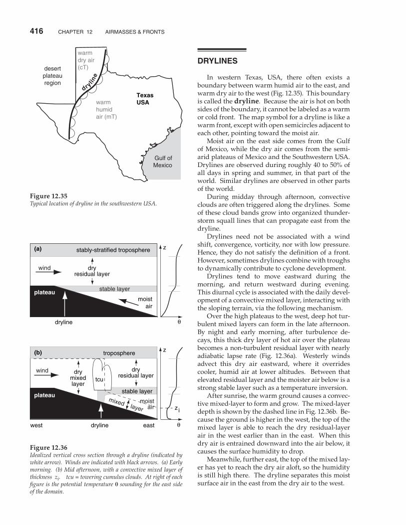
416 CHAPTEr 12 AirMASSES & FrONTS
Drylines
In western Texas, USA, there often exists a boundary between warm humid air to the east, and warm dry air to the west (Fig. 12.35). This boundary is called the dryline. Because the air is hot on both sides of the boundary, it cannot be labeled as a warm or cold front. The map symbol for a dryline is like a warm front, except with open semicircles adjacent to each other, pointing toward the moist air. Moist air on the east side comes from the Gulf of Mexico, while the dry air comes from the semi-arid plateaus of Mexico and the Southwestern USA. Drylines are observed during roughly 40 to 50% of all days in spring and summer, in that part of the world. Similar drylines are observed in other parts of the world. During midday through afternoon, convective clouds are often triggered along the drylines. Some of these cloud bands grow into organized thunder-storm squall lines that can propagate east from the dryline. Drylines need not be associated with a wind shift, convergence, vorticity, nor with low pressure. Hence, they do not satisfy the definition of a front. However, sometimes drylines combine with troughs to dynamically contribute to cyclone development. Drylines tend to move eastward during the morning, and return westward during evening. This diurnal cycle is associated with the daily devel-opment of a convective mixed layer, interacting with the sloping terrain, via the following mechanism. Over the high plateaus to the west, deep hot tur-bulent mixed layers can form in the late afternoon. By night and early morning, after turbulence de-cays, this thick dry layer of hot air over the plateau becomes a non-turbulent residual layer with nearly adiabatic lapse rate (Fig. 12.36a). Westerly winds advect this dry air eastward, where it overrides cooler, humid air at lower altitudes. Between that elevated residual layer and the moister air below is a strong stable layer such as a temperature inversion. After sunrise, the warm ground causes a convec-tive mixed-layer to form and grow. The mixed-layer depth is shown by the dashed line in Fig. 12.36b. Be-cause the ground is higher in the west, the top of the mixed layer is able to reach the dry residual-layer air in the west earlier than in the east. When this dry air is entrained downward into the air below, it causes the surface humidity to drop. Meanwhile, further east, the top of the mixed lay-er has yet to reach the dry air aloft, so the humidity is still high there. The dryline separates this moist surface air in the east from the dry air to the west.
Figure 12.35Typical location of dryline in the southwestern USA.
Figure 12.36Idealized vertical cross section through a dryline (indicated by white arrow). Winds are indicated with black arrows. (a) Early morning. (b) Mid afternoon, with a convective mixed layer of thickness zi. tcu = towering cumulus clouds. At right of each figure is the potential temperature θ sounding for the east side of the domain.

r. STULL • METEOrOLOGy FOr SCiENTiSTS AND ENGiNEErS 417
As the day continues, the mixed layer in the moist air deepens, allowing the region of dry-air entrain-ment to spread eastward. This causes the dryline to move eastward as the day progresses. At night, convective turbulence ceases, a stable boundary lay-er develops, and prevailing low-altitude easterlies advect moist air back toward the west (Fig. 12.36a). If we assume that initially the inversion is lev-el with respect to sea level, then using geometry, we can see that the progression speed of the dry-line eastward ∆x/∆t is directly related to the rate of growth of the mixed layer ∆zi/∆t :
∆∆
=∆ ∆x
tz t
si /
(12.13)
where s = ∆z/∆x is the terrain slope. Suppose the early morning stable boundary lay-er has a linear profile of potential temperature γ = ∆θ/∆z, then the mixed-layer growth proceeds with the square-root of accumulated daytime heating QAk (see the Atmospheric Boundary Layer chapter):
zQ
iAk=
21 2
·/
γ (12.14)
As a result, the distance ∆x that a dryline moves eastward as a function of time is:
∆ =
xs
QAk1 21 2
··
/
γ (12.15)
Time is hidden in the cumulative heat term QAk.
sUMMary
Surface fronts mark the boundaries between air-masses. Changes in wind, temperature, humidity, visibility, and other meteorological variables are frequently found at fronts. Along frontal zones are often low clouds, low pressure, and precipitation. Fronts rotate counterclockwise around the lows in the Northern Hemisphere as the lows move and evolve. Fronts strengthen or weaken due to advection by the wind (kinematics), external diabatic heating (thermodynamics), and ageostrophic cross-frontal circulations (dynamics). One measure of frontal strength is the temperature change across it. The spread of cold air behind a front is constrained by Coriolis force, as winds adjust toward geostrophic. Airmasses can form when air resides over a sur-face sufficiently long. This usually happens in high-pressure centers of light wind. Airmasses over cold surfaces take longer to form than those over warmer
Solved Example (§) Suppose the surface heat flux during the day is constant with time at 0.2 K·m/s in the desert south-west USA. The early morning sounding has a poten-tial temperature gradient of γ = 10 K/km. The terrain slope is 1:400. Plot the dryline position with time.
SolutionGiven: γ = 10 K/km, s = 1/400, FH = 0.2 K·m/s, Find: ∆x(t) = ? km.
For constant surface flux, cumulative heating is:
Q F tAk H= ∆·
where ∆t is time since sunrise.
Thus, eq. (12.15) can be rewritten as:
∆ =∆
=∆
xs
F tH1 2
4001
2 0 2
1 2
·· ·
··( . )·
/
γ
K ·m/s tt( . )
/
0 01
1 2
K/m
Plotting this with a spreadsheet program:
Check: Units OK. Physics OK. Graph reasonable.Discussion: The dryline moves to the east with the square-root of time. Thus, the further east it gets, the slower it goes.

418 CHAPTEr 12 AirMASSES & FrONTS
exerCises
numerical problemsN1. Identify typical characteristics of the following airmass: a. cAA b. cP c. cT d. cM e. cE f. mA g. mP h. mT i. mM j. mE k. cEw l. cAk m. cPw n. mPk o. mTw
N2. List all the locations in the world where the fol-lowing airmasses typically form. a. cAA b. cA c. cP d. mP e. mT f. cT g. mE
N3.(§) Produce a graph of warm airmass depth zi and airmass potential temperature θML as a func-tion of time, similar to Fig. 12.5. Use all the same conditions as in that figure (γ = 3.3 K/km, β = 10–6 s–1, initial ∆θs = 10°C; see the solved example on the subsequent page) for genesis of a warm airmass, ex-cept with the following changes: a. initial ∆θs = 5°C b. initial ∆θs = 15°C c. initial ∆θs = 20°C d. initial ∆θs = 15°C e. β = 0 s–1 f. β = 10–7 s–1
g. β = 5 x 10⁻⁷ s–1 h. β = 5 x 10⁻⁶ s–1
i. β = 10–5 s–1 j. γ = 5 K/km k. γ = 4 K/km l. γ = 3 K/km m. γ = 2 K/km n. γ = 1 K/km
N4. Same as the previous exercise, but find the time scale τ that estimates when the peak airmass depth occurs for warm airmass genesis.
N5. For the katabatic winds of Antarctica, find the downslope buoyancy force per unit mass for this lo-cation:Location ∆z/∆x ∆θ (K) Te (K) a. Interior 0.001 40 233b. Interior 0.002 35 238c. Interior 0.003 30 243d. Intermediate 0.004 27 245e. Intermediate 0.005 25 248f. Intermediate 0.006 24 249g. Intermediate 0.007 23 250h. Coast 0.008 22 251i. Coast 0.009 21 252j. Coast 0.010 20 253k. Coast 0.011 19 254
N6.(§) An Arctic airmass of initial temperature –30°C is modified as it moves at speed 10 m/s over smooth warmer surface of temperature 0°C. As-sume constant airmass thickness. Find and plot the airmass (mixed-layer) temperature vs. downwind distance for an airmass thickness (m) of:
surfaces because turbulence is weaker in the stati-cally stable air over the cold surface. As airmasses move from their source regions, they are modified by the surfaces and terrain over which they flow. Upper-tropospheric fronts can form as folds in the tropopause. Drylines form over sloping terrain as a boundary between dry air to the west and moist air to the east; however, drylines do not usually pos-sess all the characteristics of fronts.
threads Mid-latitude highs form because of the meander-ing jet stream (Chapter 11). Formation and modifica-tion of airmasses, and dryline evolution, are caused by boundary layer (Chapter 18) processes such as turbulence. Subsidence and divergence in highs are linked by the continuity equation (Chapter 10). Air-mass modification over mountains can be estimated using thermo diagrams (Chapter 5). Geostrophic adjustment is caused by Coriolis force (Chapter 10). Isentropes (Chapter 3) can be used for frontal analy-sis. Airmasses are drawn into lows (Chapter 13), which enhances baroclinicity to strengthen the cy-clonic circulation. Highs and fronts are predicted numerically (Chapter 20) during routine weather forecasts. Cold and occluded fronts and dry lines can trigger thunderstorms (Chapters 14 and 15). Air pollution (Chapter 19) is trapped in highs, causing air stagnation events and air-pollution alerts.

r. STULL • METEOrOLOGy FOr SCiENTiSTS AND ENGiNEErS 419
a. 100 b. 200 c. 300 d. 400 e. 500 f. 600 g. 700 h. 800 i. 900 j. 1000 k. 1200 l. 1400 m. 1500
N7. Find the external Rossby radius of deformation at 60° latitude for a cold airmass of thickness 500 m and ∆θ (°C) of: a. 2 b. 4 c. 6. d. 8 e. 10 f. 12 g. 14 h. 16 i. 18 j. 20 k. 22 l. 24 m. 26 n. 28Assume a background potential temperature of 300K.
N8.(§) Find and plot the airmass depth and geo-strophic wind as a function of distance from the front for the cases of the previous exercise. Assume a background potential temperature of 300 K.
N9. Suppose that ∆θ/∆x = 0.02°C/km, ∆θ/∆y = 0.01°C/km, and ∆θ/∆z = 5°C/km. Also suppose that ∆U/∆x = – 0.03 (m/s)/km, ∆V/∆x = 0.05 (m/s)/km, and ∆W/∆x = 0.02 (cm/s)/km. Find the kinematic frontogenesis contributions from: a. confluence b. shear c. tilting d. and find the strengthening rate.
N10. A thunderstorm on the warm side of a 300 km wide front rains at the following rate (mm/h). Find the thermodynamic contribution to frontogenesis. a. 0.2 b. 0.4 c. 0.6 d. 0.8 e. 1.0 f. 1.2 g. 1.4 h. 1.6 i. 1.8 j. 2.0 k. 2.5 l. 3.0 m. 3.5 n. 4.0
N11. Plot dryline movement with time, given the following conditions. Surface heat flux is constant with time at kinematic rate 0.2 K·m/s. The verti-cal gradient of potential temperature in the initial sounding is γ. Terrain slope is s = ∆z/∆x. γ (K/km) s γ (K/km) s a. 8 1/500 b. 8 1/400 c. 8 1/300 d. 8 1/200 e. 12 1/500 f. 12 1/400 g. 12 1/300 h. 12 1/200 i. 15 1/500 j. 15 1/400
Understanding & Critical evaluationU1. Would you expect there to be a physically- or dynamically-based upper limit on the number of warm fronts and cold fronts that can extend from a low-pressure center? Why?
U2. Sketch a low with two fronts similar to Fig. 12.1, but for the Southern Hemisphere.
U3. What are the similarities and differences be-tween a ridge and a high-pressure center? Also, on a weather map, what characteristics would you look
for to determine if a weather feature is a ridge or a trough?
U4. In high-pressure centers, is the boundary-lay-er air compressed to greater density as subsidence pushes down on the top of the mixed layer? Ex-plain.
U5. In Fig. 12.3b, use the hypsometric relationship to explain why the ridge shifts or tilts westward with increasing altitude. Hint: consider where warm and cold air is relative to the surface high.
U6. How would Fig. 12.3b be different, if at all, in Southern Hemisphere mid-latitudes. Hint: Con-sider the direction that air rotates around a surface high, and use that information to describe which side of the high (east or west) advects in warm air and which advects in colder air.
U7. Consider the global-circulation, monsoon, and topographic mechanisms that can form high-pres-sure regions. Use information from the chapters on Global Circulation, Extratropical Cyclones, and Lo-cal Winds to identify 3 or more regions in the world where 2 or more of those mechanisms are super-imposed to help create high-pressure regions. De-scribe the mechanisms at each of those 3 locations, and suggest how high-pressure formation might vary during the course of a year.
U8. Out of all the different attributes of airmasses, why do you think that the airmass abbreviations listed in Table 12-1 focus on only the temperature (i.e., AA, A, P, T, M, E) and humidity (c, m)? In other words, what would make the relative temperature and humidity of airmasses be so important to weath-er forecasters? Hint: consider what you learned about heat and humidity in earlier chapters.
U9. Fig. 12.4 shows the genesis regions for many different airmasses. At first glance, this map looks cluttered. But look more closely for patterns and describe how you can anticipate where in the world you might expect the genesis regions to be for a par-ticular airmass type.
U10. In this chapter, I described two very different mechanisms by which warm and cold airmasses are created. Why would you expect them to form differ-ently? Hint: consider the concepts, not the detailed equations.
U11. Fig. 12.5 shows how initially-cold air is trans-formed into a warm airmass after it becomes parked over a warm surface such as a tropical ocean. It is
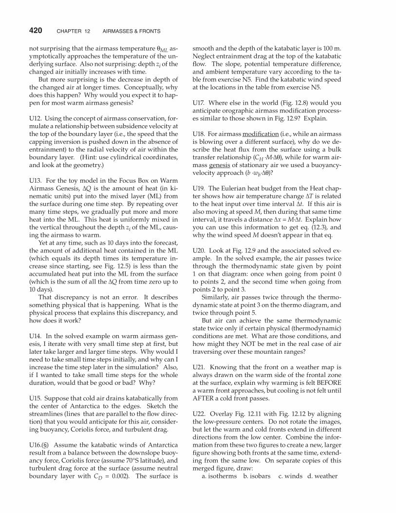
420 CHAPTEr 12 AirMASSES & FrONTS
smooth and the depth of the katabatic layer is 100 m. Neglect entrainment drag at the top of the katabatic flow. The slope, potential temperature difference, and ambient temperature vary according to the ta-ble from exercise N5. Find the katabatic wind speed at the locations in the table from exercise N5.
U17. Where else in the world (Fig. 12.8) would you anticipate orographic airmass modification process-es similar to those shown in Fig. 12.9? Explain.
U18. For airmass modification (i.e., while an airmass is blowing over a different surface), why do we de-scribe the heat flux from the surface using a bulk transfer relationship (CH ·M·∆θ), while for warm air-mass genesis of stationary air we used a buoyancy-velocity approach (b ·wb·∆θ)?
U19. The Eulerian heat budget from the Heat chap-ter shows how air temperature change ∆T is related to the heat input over time interval ∆t. If this air is also moving at speed M, then during that same time interval, it travels a distance ∆x = M·∆t. Explain how you can use this information to get eq. (12.3), and why the wind speed M doesn’t appear in that eq.
U20. Look at Fig. 12.9 and the associated solved ex-ample. In the solved example, the air passes twice through the thermodynamic state given by point 1 on that diagram: once when going from point 0 to points 2, and the second time when going from points 2 to point 3. Similarly, air passes twice through the thermo-dynamic state at point 3 on the thermo diagram, and twice through point 5. But air can achieve the same thermodynamic state twice only if certain physical (thermodynamic) conditions are met. What are those conditions, and how might they NOT be met in the real case of air traversing over these mountain ranges?
U21. Knowing that the front on a weather map is always drawn on the warm side of the frontal zone at the surface, explain why warming is felt BEFORE a warm front approaches, but cooling is not felt until AFTER a cold front passes.
U22. Overlay Fig. 12.11 with Fig. 12.12 by aligning the low-pressure centers. Do not rotate the images, but let the warm and cold fronts extend in different directions from the low center. Combine the infor-mation from these two figures to create a new, larger figure showing both fronts at the same time, extend-ing from the same low. On separate copies of this merged figure, draw: a. isotherms b. isobars c. winds d. weather
not surprising that the airmass temperature θML as-ymptotically approaches the temperature of the un-derlying surface. Also not surprising: depth zi of the changed air initially increases with time. But more surprising is the decrease in depth of the changed air at longer times. Conceptually, why does this happen? Why would you expect it to hap-pen for most warm airmass genesis?
U12. Using the concept of airmass conservation, for-mulate a relationship between subsidence velocity at the top of the boundary layer (i.e., the speed that the capping inversion is pushed down in the absence of entrainment) to the radial velocity of air within the boundary layer. (Hint: use cylindrical coordinates, and look at the geometry.)
U13. For the toy model in the Focus Box on Warm Airmass Genesis, ∆Q is the amount of heat (in ki-nematic units) put into the mixed layer (ML) from the surface during one time step. By repeating over many time steps, we gradually put more and more heat into the ML. This heat is uniformly mixed in the vertical throughout the depth zi of the ML, caus-ing the airmass to warm. Yet at any time, such as 10 days into the forecast, the amount of additional heat contained in the ML (which equals its depth times its temperature in-crease since starting, see Fig. 12.5) is less than the accumulated heat put into the ML from the surface (which is the sum of all the ∆Q from time zero up to 10 days). That discrepancy is not an error. It describes something physical that is happening. What is the physical process that explains this discrepancy, and how does it work?
U14. In the solved example on warm airmass gen-esis, I iterate with very small time step at first, but later take larger and larger time steps. Why would I need to take small time steps initially, and why can I increase the time step later in the simulation? Also, if I wanted to take small time steps for the whole duration, would that be good or bad? Why?
U15. Suppose that cold air drains katabatically from the center of Antarctica to the edges. Sketch the streamlines (lines that are parallel to the flow direc-tion) that you would anticipate for this air, consider-ing buoyancy, Coriolis force, and turbulent drag.
U16.(§) Assume the katabatic winds of Antarctica result from a balance between the downslope buoy-ancy force, Coriolis force (assume 70°S latitude), and turbulent drag force at the surface (assume neutral boundary layer with CD = 0.002). The surface is

r. STULL • METEOrOLOGy FOr SCiENTiSTS AND ENGiNEErS 421
U23. Suppose you saw from your barometer at home that the pressure was falling. So you suspect that a front is approaching. What other clues can you use (by standing outside and looking at the clouds and weather; NOT by looking at the TV, computer, or other weather instruments) to determine if the ap-proaching front is a warm or cold front. Discuss, along with possible pitfalls in this method.
U24. Draw new figures (a) - (d) similar to (a) - (d) in Figs. 12.11 and 12.12, but for an occluded front.
U25. Use the columns of temperature data in Fig. 12.13a, and plot each column as a separate sound-ing on a thermo diagram (See the Stability chapter for blank thermo diagrams that you can photocopy for this exercise. Use a skew-T diagram, unless your instructor tells you otherwise). Describe how the frontal zone shows up in the soundings.
U26. Draw isentropes that you might expect in a vertical cross-section through a warm front.
U27. Other than drylines, is it possible to have fronts with no temperature change across them? How would such fronts be classified? How would they behave?
U28. What clouds and weather would you expect with a cold anafront?
U29. Why should the Rossby radius of deformation depend on the depth of the cold airmass in a geo-strophic adjustment process?
U30. For geostrophic adjustment, the initial outflow of cold air turns, due to Coriolis force, until it is par-allel to the front. Why doesn’t it continue turning and point back into the cold air?
U31. For geostrophic adjustment, what is the nature of the final winds, if the starting point is a shallow cylinder of cold air 2 km thick and 500 km radius?
U32. Starting with Fig. 12.18, suppose that ABOVE the bottom contoured surface the temperature is horizontally uniform. Redraw that diagram but with the top two contoured surfaces sloped appro-priately for the new temperature state.
U33. By inspection, write a kinematic frontogenesis equation (similar to eq. 12.10), but for an east-west aligned front.
U34. Figs. 12.22 - 12.24 presume that temperature gradients already exist, which can be strengthened by kinematic frontogenesis. Is that presumption valid for Earth’s atmosphere? Justify.
U35. For the fronts analyzed in the Solved Example in the section on Surface Fronts – Horizontal Struc-ture, estimate and compare magnitudes of any kine-matic, thermodynamic, and dynamic processes that might exist across those fronts, based on the plotted weather data (which includes info on winds, precip-itation, etc.). Discuss the relative importance of the various mechanisms for frontogenesis.
U36. Speculate on which is more important for dy-namically generating ageostrophic cross-frontal cir-culations: the initial magnitude of the geostrophic wind or the change of geostrophic wind.
U37. What happens in an occluded front where the two cold air masses (the one advancing behind the cold front, and the one retreating ahead of the warm front) have equal virtual temperature?
U38. Draw isentropes that you expect in a vertical cross-section through a cold front occlusion (where a cold front catches up to a warm front), and discuss the change of static stability across this front.
U39. What types of weather would be expected with an upper-tropospheric front that does not have an associated surface front? [Hint: track movement of air parcels as they ride isentropic surfaces.]
U40. Draw a sketch similar to Fig. 12.34 showing the transverse circulations, but for a vertical cross-sec-tion in the Southern Hemisphere.
U41. Would you expect drylines to be possible in parts of the world other than the S.W. USA? If so, where? Justify your arguments.
Web-enhanced QuestionsW1. Monitor the weather maps on the web every day for a week or more during N. Hemisphere winter, and make a sketch of each low center with the fronts extending (similar to Fig. 12.1). Discuss the variety of arrangements of warm, cold, and occluded fronts that you have observed during that week.
W2. Same as W1, but for the S. Hemisphere during S. Hemisphere winter.
W3. On a surface weather map, identify high-pres-sure centers, and identify ridges. Also, on a 50 kPa

422 CHAPTEr 12 AirMASSES & FrONTS
W11. Access a sequence of weather maps that cover a large spatial area, with temporal coverage every 6 or 12 h for a week. Find an example of a front that you can follow from beginning (frontogenesis) through maturity to the end (frontolysis). Discuss how the front moves as it evolves, and what the time scale for its evolution is.
W12. Print from the web a weather map that shows both the analyzed fronts and the station plot data. On this map, draw your own analysis of the data to show where the frontal zones are. Discuss how the weather characteristics (wind, pressure, tempera-ture, weather) across these real fronts compare with the idealized sketches of Figs. 12.11 and 12.12.
W13. Access a sequence of surface weather maps from the web that show the movement of fronts. Do you see any fronts that are labeled as stationary fronts, but which are moving? Do you see any fronts labeled as warm or cold fronts, but which are not moving? Are there any fronts that move backwards compared to the symbology labeling the front (i.e., are the fronts moving opposite to the direction that the triangles or semicircles point)? [Hint: often fronts are designated by how they move relative to the low center. If a cold front, for example, is advanc-ing cyclonically around a low, but the low is moving toward the west (i.e., backwards in mid-latitudes), then relative to people on the ground, the cold front is retreating.]
W14. Access weather map data that shows a strong cold front, and compare the winds on both sides of that front to the winds that you would expect using geostrophic-adjustment arguments. Discuss.
W15. For a wintertime situation, access a N. (or S.) Hemisphere surface weather map from the web, or access a series of weather maps from different agen-cies around the world in order to get information for the whole Hemisphere. Draw the location of the polar front around the globe.
W16. Access weather maps from the web that show a strengthening cold or warm front. Use the other weather data on this map to suggest if the strength-ening is due mostly to kinematic, thermodynamic, or dynamic effects.
W17. Access a sequence of weather maps that shows the formation and evolution of an occluded front. Determine if it is a warm or cold occlusion (you might need to analyze the weather map data by hand to help you determine this).
(500 hPa) chart, do the same. Look at the ratio of ridges to high centers for each chart, and identify which chart (surface or 50 kPa) has the largest rela-tive number of high centers, and which has the larg-est relative number of ridges.
W4. From weather maps showing vertical velocity w, find typical values of that vertical velocity near the center of highs. (If ω = ∆P/∆t is used instead of w, it is acceptable to leave the units in mb/s). Compare this vertical velocity to the radial velocity of air di-verging away from the high center in the boundary layer.
W5. Use a sequence of surface weather maps every 6 or 12 h for a week, where each map spanning a large portion of the globe. Find one or more locations that exhibits the following mechanism for formation of a surface high pressure: a. global circulation b. monsoon c. Rossby wave d. thunderstorm e. topographic
W6. Do a web search to find surface weather maps that also include airmass abbreviations on them. Print one of these maps, and suggest how the la-beled airmass moved to its present location from its genesis region (where you will need to make a rea-sonable guess as to where its genesis region was).
W7. Use weather maps on the web to find a loca-tion where air has moved over a region and then becomes stationary. Monitor the development of a new airmass (or equivalently, modification of the old airmass) with time at this location. Look at tempera-ture and humidity.
W8. For a weather situation of relatively zonal flow from west to east over western N. America, access upper air soundings for weather stations in a line more-or-less along the wind direction. Show how the sounding evolves as the air flows over each ma-jor mountain range. How does this relate to airmass modification?
W9. Access upper air soundings for a line of RAOB stations across a front. Use this data to draw vertical cross-sections of: a. pressure or height b. temperature c. humidity d. potential temperature
W10. Same as previous exercise, but identify the frontal inversions (or frontal stable layers) aloft in the soundings.

r. STULL • METEOrOLOGy FOr SCiENTiSTS AND ENGiNEErS 423
W18. Use the web to access a 3-D sketch of a TROW-AL. Use this and other web sites to determine other characteristics of TROWALs.
W19. Download upper-air soundings from a station under or near the jet stream. Use the data to see if there is a tropopause fold. [Hint: assuming that you don’t have measurements of radioactivity or isentropic potential vorticity, use mixing ratio or po-tential temperature as a tracer of stratospheric air.]
W20. Search the web for surface weather maps that indicate a dryline in the S.W. USA. If one exists, then search the web for upper-air soundings just east and just west of the dryline. Plot the resulting soundings of potential temperature and humidity, and discuss how it relates to the idealized sketch of a dryline in this textbook.
synthesis QuestionsS1. Fig. 12.2 shows a ridge that is typical of mid-lati-tudes in the N. Hemisphere. Sketch a ridge for: a. Southern Hemisphere mid-latitudes b. N. Hemisphere tropics c. S. Hemisphere tropicsHint: Consider the global pressure patterns de-scribed in the Global Circulation chapter.
S2. What if there was no inversion at the top of the boundary layer? Redraw Fig. 12.3a for this situa-tion.
S3. What if the Earth had no oceans? What mecha-nisms could create high-pressure centers and/or high-pressure belts?
S4. For your location, rank the importance of the different mechanisms that could create highs, and justify your ranking.
S5. Airmasses are abbreviated mostly by the rela-tive temperature and humidity associated with their formation locations. Table 12-1 also describes two other attributes: returning airmasses, and airmass-es that are warmer or colder than the underlying surface. What one additional attribute would you wish airmasses could be identified with, to help you to predict the weather at your location? Explain.
S6. Fig. 12.4 shows many possible genesis regions for airmasses. But some of these regions would not likely exist during certain seasons, because of the ab-sence of high-pressure centers. For the hemisphere (northern or southern) where you live, identify how the various genesis regions appear or disappear with the seasons. Also, indicate the names for any
of the high-pressure centers. For those that exist year round, indicate how they shift location with the seasons. (Hint: review the global circulation info in the Global Circulation chapter.)
S7. What if airmasses remained stationary over the genesis regions forever? Could there be fronts and weather? Explain.
S8. Would it be possible for an airmass to become so thick that it fills the whole troposphere? If so, ex-plain the conditions needed for this to occur.
S9. What if boundary-layer processes were so slow that airmasses took 5 times longer to form compared to present airmass formation of about 3 to 5 days? How would the weather and global circulation be different, if at all?
S10. Cold-air drainage from Antarctica is so strong and persistent that it affects the global circulation. Discuss how this affect is captured (or not) in the global maps in the Global Circulation chapter.
S11. What if Antarctica was flat, similar to the Arc-tic? How would airmasses and Earth’s climate be different, if at all?
S12. Consider Fig. 12.8. How would airmass forma-tion and weather be different, if at all, given: a. Suppose the Rocky Mountains disappeared, and a new dominant mountain range (named after you), appeared east-west across the middle of N. America. b. Suppose that the Alps and Pyrenees dis-appeared and were replaced by a new dominant north-south mountain range (named after you) go-ing through Europe from Copenhagen to Rome. c. Suppose no major mountain ranges existed.
S13. Suppose a cross-section of the terrain looked like Fig. 12.9, except that the Great Basin region were below sea level (and not flooded with water). Describe how airmass modification by the terrain would be different, if at all.
S14. What if precipitation did not occur as air flows over mountain ranges? Thus, mountains could not modify air masses by this process. How would weather and climate be different from now, if at all?
S15. A really bad assumption was made in eq. (12.3); namely, zi = constant as the airmass is modified. A better assumption would be to allow zi to change with time (i.e., with distance as it blows over the new surface). The bad assumption was made because it
424 CHAPTEr 12 AirMASSES & FrONTS
allowed us to describe the physics with a simple eq. (12.3), which could be solved analytically to get eq. (12.4). This is typical of many physical problems, where it is impossible to find an exact analytical so-lution to the full equations describing true physics (as best we know it). So here is a philosophical question. Is it better to approximate the physics to allow an exact analytical solution of the simplified problem? Or is it better to try to get an approximate (iterated or graphical solu-tion) to the exact, more-complicated physics? Weigh the pros and cons of each approach, and discuss.
S16. For a (a) cold front, or a (b) warm front, create station plot data for a weather station 100 km ahead of the front, and for another weather station 100 km behind the front. Hint: use the sketches in Figs. 12.11 and 12.12 to help decide what to plot.
S17. Suppose the width of frontal zones were in-finitesimally small, but their lengths remained un-changed. How would weather be different, if at all?
S18. What if turbulence were always so intense that frontal zones were usually 1000 km in width? How would weather be different, if at all?
S19. Does the geostrophic adjustment process affect the propagation distance of cold fronts in the real atmosphere, for cold fronts that are imbedded in the cyclonic circulation around a low-pressure center? If this indeed happens, how could you detect it?
S20. The boxes at the top of Figs. 12.22 - 12.24 show the associated sign of key terms for kinematic frontogenesis. If those terms have opposite signs, draw sketches similar to those figures, but showing frontolysis associated with: a. confluence b. shear c. tilting.
S21. Suppose that condensation of water vapor caused air to cool. How would the thermodynamic mechanism for frontogenesis work for that situa-tion, if at all? How would weather be near fronts, if at all?
S22. Suppose that ageostrophic motions were to ex-perience extremely large drag, and thus would tend to dissipate quickly. How would frontogenesis in Earth’s atmosphere be different, if at all?
S23. After cold frontal passage, cold air is moving over ground that is still warm (due to its thermal inertia). Describe how static stability varies with height within the cold airmass 200 km behind the cold front. Draw thermo diagram sketches to illus-trate your arguments.
S24. Suppose a major volcanic eruption injected a thick layer of ash and sulfate aerosols at altitude 20 km. Would the altitude of the tropopause adjust to become equal to this height? Discuss.
S25. Suppose the slope of the ground in a dryline situation was not as sketched in Fig. 12.36. Instead, suppose the ground was bowl-shaped, with high plateaus on both the east and west ends. Would drylines exist? If so, what would be their character-istics, and how would they evolve?