msc qt: statistics part ii statistical inference (weeks … qt: statistics part ii statistical...
TRANSCRIPT
MSc QT: StatisticsPart II Statistical Inference
(Weeks 3 and 4)
Roald J. VersteegDepartment of Economics, Mathematics and Statistics
Malet Street, London WC1E 7HX
September 2014
MSc Economics & MSc Financial Economics (FT & PT2)MSc Finance & MSc Financial Risk Management (FT & PT2)
MSc Financial Engineering (FT & PT1)PG Certificate in Econometrics (PT1)

Contents
Introduction v
1 Sampling Distributions 1Literature . . . . . . . . . . . . . . . . . . . . . . . . . . . . . . . . . . . . . . . . . . 11.1 Introduction . . . . . . . . . . . . . . . . . . . . . . . . . . . . . . . . . . . . . . 11.2 Sampling Distributions . . . . . . . . . . . . . . . . . . . . . . . . . . . . . . . . 21.3 Sampling Distributions Derived from the Normal . . . . . . . . . . . . . . . . . . 7
1.3.1 Chi-Square . . . . . . . . . . . . . . . . . . . . . . . . . . . . . . . . . . 71.3.2 Student-t . . . . . . . . . . . . . . . . . . . . . . . . . . . . . . . . . . . 81.3.3 F-distribution . . . . . . . . . . . . . . . . . . . . . . . . . . . . . . . . . 9
Problems . . . . . . . . . . . . . . . . . . . . . . . . . . . . . . . . . . . . . . . . . . 10
2 Large Sample Theory 13Literature . . . . . . . . . . . . . . . . . . . . . . . . . . . . . . . . . . . . . . . . . . 132.1 Law of Large Numbers . . . . . . . . . . . . . . . . . . . . . . . . . . . . . . . . 132.2 The Central Limit Theorem . . . . . . . . . . . . . . . . . . . . . . . . . . . . . . 18Problems . . . . . . . . . . . . . . . . . . . . . . . . . . . . . . . . . . . . . . . . . . 19
3 Estimation 21Literature . . . . . . . . . . . . . . . . . . . . . . . . . . . . . . . . . . . . . . . . . . 213.1 Introduction . . . . . . . . . . . . . . . . . . . . . . . . . . . . . . . . . . . . . . 213.2 Evaluation Criteria for Estimators . . . . . . . . . . . . . . . . . . . . . . . . . . 223.3 Confidence Intervals . . . . . . . . . . . . . . . . . . . . . . . . . . . . . . . . . 23Problems . . . . . . . . . . . . . . . . . . . . . . . . . . . . . . . . . . . . . . . . . . 27
4 Hypothesis Testing 29Literature . . . . . . . . . . . . . . . . . . . . . . . . . . . . . . . . . . . . . . . . . . 294.1 Introduction . . . . . . . . . . . . . . . . . . . . . . . . . . . . . . . . . . . . . . 294.2 The Elements of a Statistical Test . . . . . . . . . . . . . . . . . . . . . . . . . . . 294.3 Duality of Hypothesis Testing and Confidence Intervals . . . . . . . . . . . . . . . 344.4 Attained Significance Levels: P-Values . . . . . . . . . . . . . . . . . . . . . . . . 354.5 Power of the Test . . . . . . . . . . . . . . . . . . . . . . . . . . . . . . . . . . . 36Problems . . . . . . . . . . . . . . . . . . . . . . . . . . . . . . . . . . . . . . . . . . 38
iii

iv QT 2014: Statistical Inference
A Exercise Solutions 41A.1 Sampling Distributions . . . . . . . . . . . . . . . . . . . . . . . . . . . . . . . . 41A.2 Large Sample Theory . . . . . . . . . . . . . . . . . . . . . . . . . . . . . . . . . 42A.3 Estimation . . . . . . . . . . . . . . . . . . . . . . . . . . . . . . . . . . . . . . . 42A.4 Hypothesis Testing . . . . . . . . . . . . . . . . . . . . . . . . . . . . . . . . . . 46
Introduction
Course Content
This part of the course consists of five lectures, followed by a closed book exam. The topics coveredare
1. Sampling distributions.
2. Large sample theory.
3. Estimation.
4. Hypothesis Testing.
The last lecture will cover exercises based on the topics above.
Textbooks
Lecture notes are provided, however these notes are not a substitute for a textbook. The requiredtextbook for this part of the course is.
• Wackerly, D., Mendenhall, W. and Schaeffer, R. (2008). Mathematical Statistics with Appli-cations, 7th ed., Cengage. (Henceforth WMS)
Students who desire a more advanced treatment of the materials might want to consider:
• Casella, G. and Berger, R. (2001). Statistical Inference, 2nd ed., Duxbury press. (HenceforthCB)
• Rice, J. (2006). Mathematical Statistics and Data Analysis, 3rd. ed., Cengage. (HenceforthR)
Furthermore, the following books are recommended for students that plan to take further coursesin econometrics. The appendices of these books also contain summaries of the material covered inthis class.
• Greene, W. (2011). Econometric Analysis, 7th ed., Prentice-Hall. (Henceforth G)
• Verbeek, M. (2012). A Guide to Modern Econometrics, 4th ed., Wiley. (Henceforth V)
v

vi QT 2014: Statistical Inference
Online Resources
The primary resources for this part of the course are contained in this syllabus. However, furtherresources can be found online at either www.ems.bbk.ac.uk/for_students/presess/ and thecourse page at the virtual learning environment Moodle (login via moodle.bbk.ac.uk/ )
Instructor
The instructor for this part of this course is
• Roald Versteeg, [email protected]

Chapter 1
Sampling Distributions
Literature
Required Reading
• WMS, Chapter 7.1 – 7.2
Recommended Further Reading
• WMS, Chapters 4 and 12
• CB, Chapter 5.1 – 5.4
• R, Chapters 6 – 7
1.1 Introduction
A statistical investigation normally starts with some measures of interest of a distribution. Thetotality of elements about which some information is desired is called a population. Often we onlyuse a small proportion of a population, known as a sample, because it is impractical to gather dataon the whole population. We measure the attributes of this sample and draw conclusions or makepolicy decisions based on the data obtained. That is, with statistical inference we estimate theunknown parameters underlying the statistical distributions of the sample. We can then measuretheir precision, test hypotheses on them to and use them to generate forecasts.
PopulationA population (of size N), x1, x2 . . . , xN is the totality of elements that we are interested in.The numerical characteristics of a population are called parameters. Parameters are oftendenoted by Greek letters such as θ.
Definition 1.1.
1

2 QT 2014: Statistical Inference
SampleA sample (of size n) is a set of random variables, X1, X2, . . . , Xn, that are drawn from thepopulation. The realization of the sample is denoted by x1, . . . , xn.
Definition 1.2.
The method of sampling, known sometimes as the design of the experiment, will affect thestructure of the data that you measure, and thus the amount of information and the likelihood ofobserving a certain sample outcome. The type of sample you collect may have profound effects onthe way you can make inferences based on that sample. For the moment we will concern ourselvesonly with the most basic of sampling methods simple random sampling.
Random SampleThe random variables X1, · · · , Xn are called a random sample of size n from the populationf (x) if X1, · · · , Xn are mutually independent random variables and the marginal pdf or pmfof each Xi is the same function f (x). Alternatively X1, · · · , Xn are called independent andidentically distributed variables with pdf of pmf f (x). This is commonly abbreviated toiid random variables.The joint density of the realized xi’s in a random sample sample has the form:
f (x1, x2, · · · , xn) =
n∏i=1
fXi(xi) (by independence)
=
n∏i=1
f (xi) (by identicality). (1.1)
Definition 1.3.
Of course, in economics and finance one normally does not have much control on how the data iscollected and the data at hand is often time-series data, which is in most cases neither independentnor identically distributed. Although addressing these issues is extremely important in empiricalanalysis, this course will ignore such considerations to focus on the basic issues.
1.2 Sampling Distributions
When drawing a sample from a population, a researcher is normally interested in reducing the datainto some summary measures. Any well-defined measure may be expressed as a function of therealized values of the sample. As the function will be based on a vector of random variables, thefunction itself, called a statistic, will be a random variable as well.

1. Sampling Distributions 3
Statistic and Sampling DistributionLet X1, . . . , Xn be a sample of size n and T (x1, . . . , xn) be a real-valued or vector-valuedfunction whose domain includes the sample space of (X1, . . . , Xn), that does not includeany unknown parameters, then the random variable X = T (x1, . . . , xn) is called a statistic.
The probability distribution of a statistic is called the sampling distribution of X.
Definition 1.4.
The analysis of these statistics and their sampling distributions is at the very core of economet-rics. As the definition of a statistic is very broad, it can include a wide range of different measures.The most two common statistics are probably the mean X and the sample variance S 2. Other statis-tics may measure the largest observation in the sample X(n), the median X(n/2), or a correlationbetween two sequences of random variables Corr(X,Y). Statistics do not need to be scalar, but mayalso be vector-valued, returning for instance all the unique values observed in the sample.
Also note the important difference between the sampling distribution which measures the proba-bility distribution of the statistic T (x1, . . . , xn) and the distribution of the population, which measuresthe marginal distribution of each Xi.
The following two sections consider the sampling distributions of the two most important statis-tics, the sample mean and the sample variance, on the assumption that the sample is drawn froma normal population. The main features of these sampling distributions are summarized by thefollowing theorem.
The sample mean and the sample variance of a random normal sample have the followingthree characteristics:
1. E[X] = µ, and sampling distribution X ∼ N(µ, σ2/n),
2. E[S 2] = σ2, and sampling distribution (n − 1)S 2/σ2 ∼ χ2n−1,
3. X and S 2 are independent random variables.
Theorem 1.5.
As some of the most common statistics, such as the sample mean and sample total are linearcombinations of the individual sample points, the following theorem is of great value in determiningthe sampling distribution of statistics.
4 QT 2014: Statistical Inference
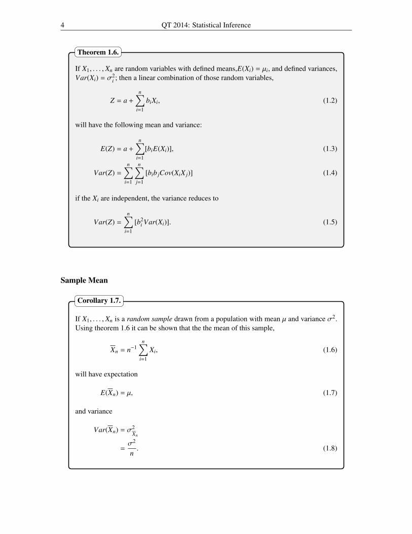
If X1, . . . , Xn are random variables with defined means,E(Xi) = µi, and defined variances,Var(Xi) = σ2
i ; then a linear combination of those random variables,
Z = a +
n∑i=1
biXi, (1.2)
will have the following mean and variance:
E(Z) = a +
n∑i=1
[biE(Xi)], (1.3)
Var(Z) =
n∑i=1
n∑j=1
[bib jCov(XiX j)] (1.4)
if the Xi are independent, the variance reduces to
Var(Z) =
n∑i=1
[b2i Var(Xi)]. (1.5)
Theorem 1.6.
Sample Mean
If X1, . . . , Xn is a random sample drawn from a population with mean µ and variance σ2.Using theorem 1.6 it can be shown that the the mean of this sample,
Xn = n−1n∑
i=1
Xi, (1.6)
will have expectation
E(Xn) = µ, (1.7)
and variance
Var(Xn) = σ2Xn
=σ2
n. (1.8)
Corollary 1.7.

1. Sampling Distributions 5
Let us consider how a sampling distribution may look like. As an example take the case ofthe sample mean Xn of a random sample drawn from a normally distributed population. Combinedwith the knowledge that linear combinations of normal variates are also normally distributed, thesampling distribution of X will be equal to
Xn ∼ N(µ,σ2
n). (1.9)
We can now go one step further and calculate the standardized sample mean. Subtracting theexpected value, which is the population mean µ, and dividing by the (asymptotic) standard errorcreates a random variable with a standard normal distribution:
Z =Xn − µ
σ/√
n∼ N(0, 1). (1.10)
Of course, in reality one does not generally know σ, in which case it is common practice toreplace it with it’s sample counterpart S , which will give the following sampling distribution:
Z =Xn − µ
S/√
n∼ tn. (1.11)
The details on why the sampling distribution changes from from a normal to a t-distribution arediscussed in the next section.
Sample Variance
If X1, . . . , Xn is a random sample drawn from a population with mean µ and variance σ2,then the sample variance
S 2n = (n − 1)−1
n∑i=1
(Xi − Xn)2, (1.12)
will have the following expectation:
E(S 2) = σ2. (1.13)
Note that to calculate the sample variance we divide by n − 1 and not n.If the sample is random and drawn from a normal population, then it can also be shownthat the sampling distribution is as follows:
(n − 1)S 2/σ2 ∼ χ2n−1. (1.14)
An intuition of this result is provided in WMS; the proof can be found in e.g. Casella andBerger, chapter 5.
Corollary 1.8.

6 QT 2014: Statistical Inference
To prove that the sample variance S 2 has expectation σ2, note that
S 2n = (n − 1)−1
n∑i=1
(Xi − Xn)2
= (n − 1)−1∑
(X2i ) − nX
2n.
Therefore, by taking expectations we get
E(S 2n) = E
[(n − 1)−1
∑(X2
i ) − nX2n
]= (n − 1)−1
(∑(E[X2
i ]) − nE[X2n])
Recall that Var(Z) = E(Z2) − E(Z)2, so
E(X2i ) = σ2 − µ2 and
E(X2n) = n−1σ2 − µ2.
Substitute to get
E(S 2n) = (n − 1)−1[n(σ2 + µ2) − n(n−1σ2 + µ2)]
= (n − 1)−1[(n − 1)σ2]
= σ2.
Proof 1.9.
Finite Population Correction
As a short distraction, notice that if the whole population is sampled, the estimation error of thesample mean will be, logically, equal to zero. Similarly, if a large proportion of the populationis sampled, without replacement, the standard error calculated above will over-estimate the truestandard error. In such cases, the standard error should be adjusted using a so-called finite populationcorrection. Taking the standard error of the sample mean as an example:
σX =
(1 −
n − 1N − 1
)σ√
n. (1.15)
When the sampling fraction n/N approaches zero, then the correction will approach 1. So formost applications,
σX ≈σ√
n, (1.16)
1. Sampling Distributions 7
which is the definition of the standard error as given in the previous section. For most samplesconsidered, the sampling fraction will be very small. Thus, the finite sample correction will beneglected throughout most of this syllabus.
1.3 Sampling Distributions Derived from the Normal
The normal distribution plays a central role in econometrics and statistics, for reasons that we willexplore in more depth in the next chapter. However, there are a number of other distributions thatfeature as sampling distributions for various (test) statistics. As it turns out, the three most commonof these distributions can actually be derived from the normal distribution.
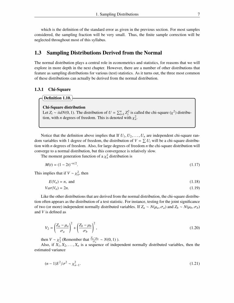
1.3.1 Chi-Square
Chi-Square distributionLet Zi ∼ iidN(0, 1). The distribution of U =
∑ni=1 Z2
i is called the chi-square (χ2) distribu-tion, with n degrees of freedom. This is denoted with χ2
n.
Definition 1.10.
Notice that the definition above implies that If U1,U2, . . . ,Un are independent chi-square ran-dom variables with 1 degree of freedom, the distribution of V =
∑Ui will be a chi-square distribu-
tion with n degrees of freedom. Also, for large degrees of freedom n the chi-square distribution willconverge to a normal distribution, but this convergence is relatively slow.
The moment generation function of a χ2n distribution is
M(t) = (1 − 2t)−n/2. (1.17)
This implies that if V ∼ χ2n, then
E(Vn) = n, and (1.18)
Var(Vn) = 2n. (1.19)
Like the other distributions that are derived from the normal distribution, the chi-square distribu-tion often appears as the distribution of a test statistic. For instance, testing for the joint significanceof two (or more) independent normally distributed variables. If Za ∼ N(µa, σa) and Zb ∼ N(µb, σb)and V is defined as
V2 =
(Za − µa
σa
)2
+
(Zb − µb
σb
)2
, (1.20)
then V ∼ χ22 (Remember that Za−µa
σa∼ N(0, 1) ).
Also, if X1, X2, . . . , Xn is a sequence of independent normally distributed variables, then theestimated variance
(n − 1)S 2/σ2 ∼ χ2n−1. (1.21)

8 QT 2014: Statistical Inference
1.3.2 Student-t
Student t distributionLet Z ∼ N(0, 1) and Un ∼ χ
2n, with Z and Un independent, then
Tn =Z
√Un/n
, (1.22)
will have a t distribution with n degrees of freedom, often denoted by tn.
Definition 1.11.
The mean an variance of a t-distribution with n degrees of freedom is
E(Tn) = 0, and (1.23)
Var(T ) =n
n − 2, n > 2. (1.24)
Like the normal, the expected value of the t-distribution is 0, and the distribution is symmetricaround it’s mean, implying that f (t) = f (−t). In contrast to the normal, the t distribution has moreprobability mass in it’s tails, a property called fat-tailness. As the degree of freedom, n, the tailsbecome lighter.
Indeed in appearance the student t distribution is very similar to the normal distribution; actuallyin the limit n −→ ∞ the t distribution converges in distribution to a standard normal distribution.Already for values of n as small as 20 or 30, the t distribution is very similar to a standard normal.
Remember that for a random sample drawn from a normal distribution, Z = (X − µ)/(σ/√
n) ∼N(0, 1). However in reality we do not have information about σ; thus we normally substitute thesample estimate
√(S 2) = S for σ. The resulting test statistic T = (X − µ)/(S/
√n) will have a
t-distribution.

1. Sampling Distributions 9
To prove T = (X − µ)/(S/√
n) ∼ t(n − 1) rewrite the statistic to get:
X − µS/√
n=
X − µS/√
n×σ/√
nσ/√
n(1.25)
=(X − µ)/(σ/
√n)
(S/√
n)/(σ/√
n)
=Z
S/σ
=Z√
S 2/σ2
=Z√
S 2/σ2 × (n − 1)/(n − 1)
=Z√
(n−1)S 2/σ2
n−1
=Z√Un−1n−1
,
where
Z = (X − µ)/(σ/√
n) ∼ N(0, 1) and
Un−1 = (n − 1)S 2/σ2 ∼ χ2n−1. (1.26)
Thus
X − µS n/√
n∼ tn−1 (1.27)
Proof 1.12.
1.3.3 F-distribution
F distributionLet Un ∼ χ
2n and Vm ∼ χ
2m, and let Un and Vm be independent from each other, then
Wn,m =Un/nVm/m
, (1.28)
will have a F distribution with m and n degrees of freedom, often denoted by Fn,m.
Definition 1.13.

10 QT 2014: Statistical Inference
The mean an variance of an F-distribution with n and m degrees of freedom is
E(Tn) =m
m − 2(1.29)
Var(T ) = 2( mm − 2
)2 n + m − 2n(m − 4)
,m > 4. (1.30)
Under specific circumstances, the F distribution converges to either a t or a χ2 distribution.Particularly
F1,m = t2m, (1.31)
and
nFn,md−→ χ2
n. (1.32)
The F-distribution often appears when investigating variances. Recall that the standardizedvariance of a normal sample will have a Chi-square distribution. Hence the ratio of two variancesof independent samples can be expressed as a F-distribution.
[(n1 − 1)S 21/σ
21]/(n1 − 1)
[(n2 − 1)S 22/σ
22]/(n2 − 1)
=S 2
1/σ21
S 22/σ
22
=Un1/n1
Vn2/n2= Fn1,n2
Problems
1. Let X1, X2, ..., Xm and Y1,Y2, ...,Yn be two normally distributed independent random samples,with Xi v N(µ1, σ
21) and Yi v N(µ2, σ
22). Suppose that µ1 = µ2 = 10, σ2
1 = 2, σ22 = 2.5, and
m = n.
(a) Find E(X) and Var(X).
(b) Find E(X − Y) and Var(X − Y).
(c) Find the sample size n, such that σ(X−Y) = 0.1.
2. Let Z1,Z2,Z3,Z4 be a sequence of independent standard normal variables. Derive distribu-tions for the following random variables.
(a) X1 = Z1 + Z2 + Z3 + Z4.
(b) X2 = Z21 + Z2
2 + Z23 + Z2
4 .
(c) X3 =Z2
1
(Z22 + Z2
3 + Z24)/3
.
(d) X4 =Z1√
Z22 + Z2
3 + Z24/√
3.
3. Indicate for each of the following statements whether they are true, false, or uncertain. Ex-plain your answer.

1. Sampling Distributions 11
(a) The variance of the sample mean is a random variable.
(b) Standard errors are negatively related to sample size.
(c) One can only do statistical inference using random samples.
(d) Let T be a rv with a student-t distribution. T 2 will have an F-distribution

12 QT 2014: Statistical Inference

Chapter 2
Large Sample Theory
Literature
Required Reading
• WMS, Chapter 7.3 – 7.6
Recommended Further Reading
• CB, Chapter 5.5
• R, Chapter 5
2.1 Law of Large Numbers
In many situations it is not possible to derive exact distributions of statistics with the use of arandom sample of observations. This problem disappears, in most cases, if the sample size is large,because we can derive an approximate distribution. Hence the need for large sample or asymptoticdistribution theory. Two of the main results of large sample theory are the Law of Large Numbers(LLN), discussed in this section, and the Central Limit Theory, described in the next section.
As large sample theory builds heavily on the notion of limits, let us first define what they are.
Limit of a sequenceSuppose a1, a2, ...., an constitute a sequence of real numbers. If there exists a real numbera such that for every real ε > 0, there exists an integer N(ε) with the property that for alln > N(ε), we have | an − a |< ε, then we say that a is the limit of the sequence {an} andwrite limn−→∞an = a.
Definition 2.1.
Intuitively, if an lies in an ε neighborhood of a (a − ε, a + ε) for all n > N(ε), then a said to bethe limit of the sequence {an}. Examples of limits are
limn−→∞
[1 +
(1n
)]= 1, and (2.1)
13

14 QT 2014: Statistical Inference
limn−→∞
[1 +
(an
)]n= ea. (2.2)
The notion of convergence is easily extended to that of a function f (x).
Limit of a functionThe function f (x) has the limit A at the point x0, if for every ε > 0 there exists a δ(ε) > 0such that | f (x) − A |< ε whenever 0 <| x − x0 |< δ(ε)
Definition 2.2.
One of the core principles in statistics is that the sample estimator will converge to the the ‘true’value when the sample gets larger. For instance, if a coin is flipped enough times, the proportion oftimes it comes up tails should get very close to 0.5. The Law of Large Numbers is a formalizationof this notion.
Weak Law of Large Numbers
The concept of convergence in probability can be used to show that, under very general conditions,the sample mean converges to the population mean, a result that is known as The Weak Law ofLarge Numbers (WLLN). This property of convergence is also referred to a consistency, will willbe treated in more detail in the next chapter.
Let X1, X2, . . . , Xn be iid random variables with E(Xi) = µ and Var(Xi) = σ2 < ∞. DefineXn = n−1 ∑n
i=1 Xi. Then for every ε > 0,
limn−→∞
Pr(|Xn − µ| < ε) = 1;
that is, Xn converges in probability to µ
Theorem 2.3 (Weak Law of Large Numbers).
As stated, the weak law of large numbers relies on the notion of convergence in probability.This type of convergence is relatively weak and so normally not too hard to verify.

2. Large Sample Theory 15
Convergence in Probabilityif
limn−→∞
Pr[| Xn − x |≥ ε] = 0 for all ε > 0,
the sequence of random variables Xn is said to converge in probability to the real numberx . We write
Xnp−→ x or plimXn = x.
Definition 2.4.
Convergence in probability implies that it becomes less and less likely that the random variable(Xn − x) lies the outside the interval (−ε,+ε) as the sample size gets larger and larger. There existdifferent equivalent definitions of convergence in probability. Some equivalent definitions are givenbelow:
1. limn−→∞ Pr[|Xn − x| < ε] = 1, ε > 0.
2. Given ε > 0 and δ > 0, there exists N(ε, δ) such that Pr[| Xn − x |> ε] < δ, for all n > N.
3. Pr[| Xn − x |< ε] > 1 − δ , for all n > N, that is, Pr[| XN+1 − x |< ε] > 1 − δ, Pr[| XN+2 − x |<ε] > 1 − δ, and so on.
If Xnp−→ X and Yn
p−→ Y , then
(a) (Xn + Yn)p−→ (X + Y),
(b) (XnYn)p−→ XY , and
(c) (Xn/Yn)p−→ X/Y (if Yn,Y , 0).
Theorem 2.5.
If g(·) is a continuous function, then Xnp−→ X implies that g(Xn)
p−→ g(X). In other
words, convergence in probability is preserved under continuous transformations.
Theorem 2.6.
The Weak Law of Large numbers can be proven by use of Chebychev’s Inequality.

16 QT 2014: Statistical Inference
Pr[g(X) ≥ ε
]≤
E[g(X)]ε
. (2.3)
For instance, let g(X) be |X − E(X)|, in this case Chebychev’s inequality reduces to
Pr[|X − E(X)|k ≥ εk
]≤
E[|X − µ|k]εk . (2.4)
Theorem 2.7 (Chebychev’s Inequality).
For every ε > 0 we have
Pr[|X − E(X)| ≥ ε
]= Pr
[(X − E(X))2 ≥ ε2
]≤
E[(X − µ)2]ε2 , (2.5)
with
E[(X − µ)2]ε2 =
Var(X)ε2
=σ2
nε2 . (2.6)
As limn−→∞( σ2
nε2 ) = 0 we have
limn−→∞
Pr[|X − E(X)| ≥ ε
]= 0. (2.7)
Proof 2.8 (Weak Law of Large Numbers).
Strong Law of Large Numbers
Like in the case of convergence in probability, almost sure convergence can be used to prove theconvergence (almost surely) of the sample mean to the population mean. This stronger result isknown as the the Strong Law of Large Numbers (SLLN).
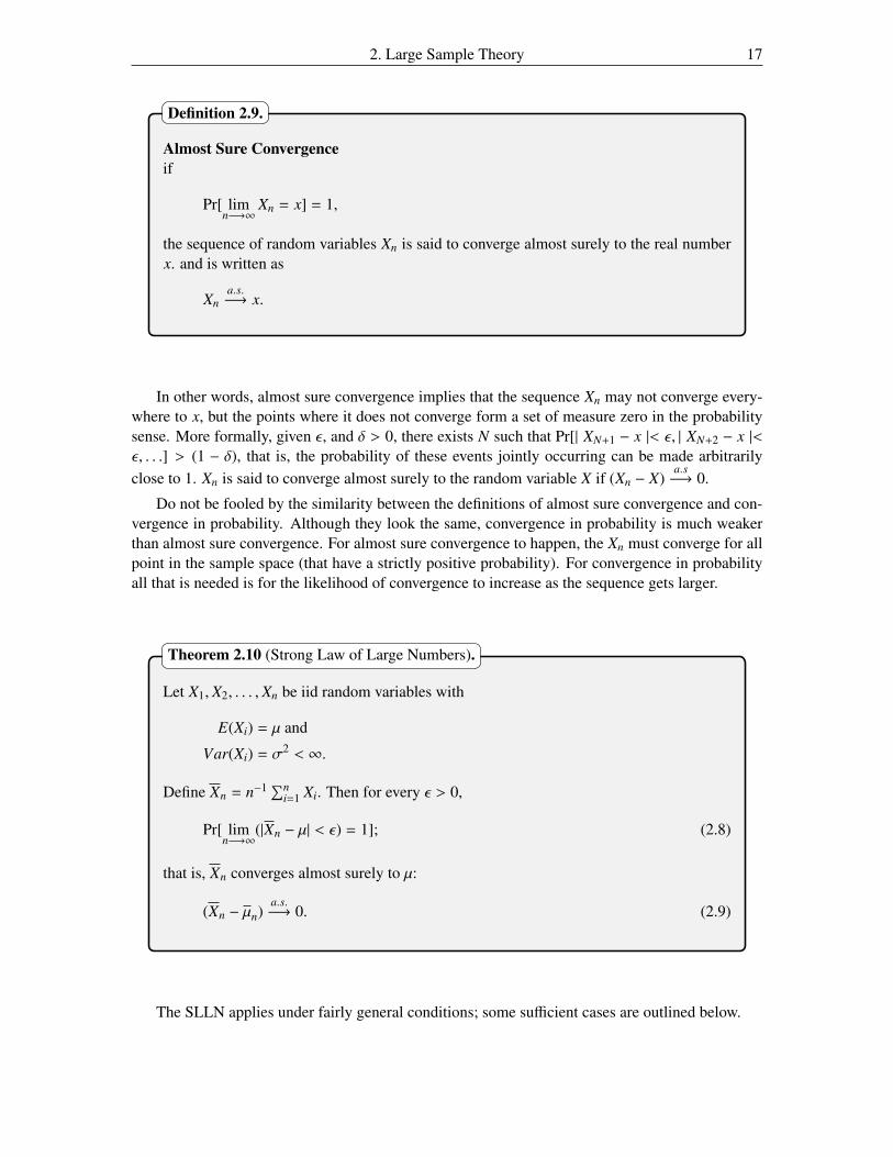
2. Large Sample Theory 17
Almost Sure Convergenceif
Pr[ limn−→∞
Xn = x] = 1,
the sequence of random variables Xn is said to converge almost surely to the real numberx. and is written as
Xna.s.−→ x.
Definition 2.9.
In other words, almost sure convergence implies that the sequence Xn may not converge every-where to x, but the points where it does not converge form a set of measure zero in the probabilitysense. More formally, given ε, and δ > 0, there exists N such that Pr[| XN+1 − x |< ε, | XN+2 − x |<ε, . . .] > (1 − δ), that is, the probability of these events jointly occurring can be made arbitrarilyclose to 1. Xn is said to converge almost surely to the random variable X if (Xn − X)
a.s−→ 0.
Do not be fooled by the similarity between the definitions of almost sure convergence and con-vergence in probability. Although they look the same, convergence in probability is much weakerthan almost sure convergence. For almost sure convergence to happen, the Xn must converge for allpoint in the sample space (that have a strictly positive probability). For convergence in probabilityall that is needed is for the likelihood of convergence to increase as the sequence gets larger.
Let X1, X2, . . . , Xn be iid random variables with
E(Xi) = µ and
Var(Xi) = σ2 < ∞.
Define Xn = n−1 ∑ni=1 Xi. Then for every ε > 0,
Pr[ limn−→∞
(|Xn − µ| < ε) = 1]; (2.8)
that is, Xn converges almost surely to µ:
(Xn − µn)a.s.−→ 0. (2.9)
Theorem 2.10 (Strong Law of Large Numbers).
The SLLN applies under fairly general conditions; some sufficient cases are outlined below.
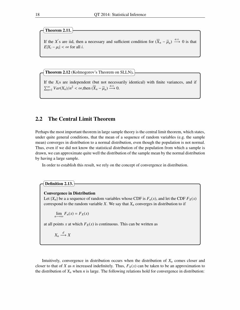
18 QT 2014: Statistical Inference
If the X′
s are iid, then a necessary and sufficient condition for (Xn − µn)a.s.−→ 0 is that
E|Xi − µi| < ∞ for all i.
Theorem 2.11.
If the Xis are independent (but not necessarily identical) with finite variances, and if∑∞n=1 Var(Xn)/n2 < ∞,then (Xn − µn)
a.s.−→ 0.
Theorem 2.12 (Kolmogorov’s Theorem on SLLN).
2.2 The Central Limit Theorem
Perhaps the most important theorem in large sample theory is the central limit theorem, which states,under quite general conditions, that the mean of a sequence of random variables (e.g. the samplemean) converges in distribution to a normal distribution, even though the population is not normal.Thus, even if we did not know the statistical distribution of the population from which a sample isdrawn, we can approximate quite well the distribution of the sample mean by the normal distributionby having a large sample.
In order to establish this result, we rely on the concept of convergence in distribution.
Convergence in DistributionLet {Xn} be a a sequence of random variables whose CDF is Fn(x), and let the CDF FX(x)correspond to the random variable X. We say that Xn converges in distribution to if
limn−→∞
Fn(x) = FX(x)
at all points x at which FX(x) is continuous. This can be written as
Xnd−→ X
Definition 2.13.
Intuitively, convergence in distribution occurs when the distribution of Xn comes closer andcloser to that of X as n increased indefinitely. Thus, FX(x) can be taken to be an approximation tothe distribution of Xn when n is large. The following relations hold for convergence in distribution:

2. Large Sample Theory 19
If Xnd−→ X and Yn
p−→ c, where c is a non-zero constant, then
(a) (Xn + Yn)d−→ (X + c), and
(b) (Xn/Yn)d−→ (X/c).
Theorem 2.14.
Using the definition of convergence in distribution we can now introduce formally the CentralLimit Theorem.
Let X1, X2, ..., Xn be iid random with mean E(Xi) = µ and a finite variance σ2 < ∞, then
Zn =Xn − E(Xn)√
Var(Xn)
=Tn − E(Tn)√
Var(Tn).
Then, under a variety of alternative assumptions
Znd−→ N(0, 1). (2.10)
Theorem 2.15 (Central Limit Theorem).
Problems
1. let X1, X2, . . . , Xn be an independent sample (i.e. independent but not identically distributed),with E(Xi) = µi and Var(Xi) = σ2
i . Also, let n−1 ∑ni=1 µi −→ µ.
Show that if n−2∑n
i=1 σ2i −→ 0, then X −→ µ in probability.
2. The service times for customers coming through a checkout counter in a retail store are inde-pendent random variables with mean 1.5 minutes and variance 1.0. Approximate the proba-bility that 100 customers can be serviced in less than 2 hours of total service time.
3. Indicate for each of the following statements whether they are true, false, or uncertain. Ex-plain your answer.
(a) If a sample from a population is large, a histogram of the values will be approximatelynormal, even if the population is not normal
(b) If a series converges almost surely to p, it will also converge in probability to p.

20 QT 2014: Statistical Inference

Chapter 3
Estimation
Literature
Required Reading
• WMS, Chapters 8 & 9.1 – 9.3
Recommended Further Reading
• R, Sections 8.6 – 8.8
• CB, Chapters 7, 9, & 10.1.
3.1 Introduction
The purpose of statistics is to use the information contained in a sample to make inference about theparameters of the population that the sample is taken from. To key to making good inference aboutthe parameters is to have a good estimation procedure that produces good estimates of the quantitiesof interest.
EstimatorAn estimator is a rule for calculating an estimate of a target parameter based on the infor-mation from a sample. To indicate the link between an estimator and it’s target parameter,say θ, the estimator is normally denoted by adding a hat: θ.
Definition 3.1.
A point estimation procedure uses the information in the sample to arrive at a single numberthat is intended to be close to the true value of the target parameter in the population. For example,the sample mean
X =
∑ni=1 Xi
n(3.1)
21
22 QT 2014: Statistical Inference
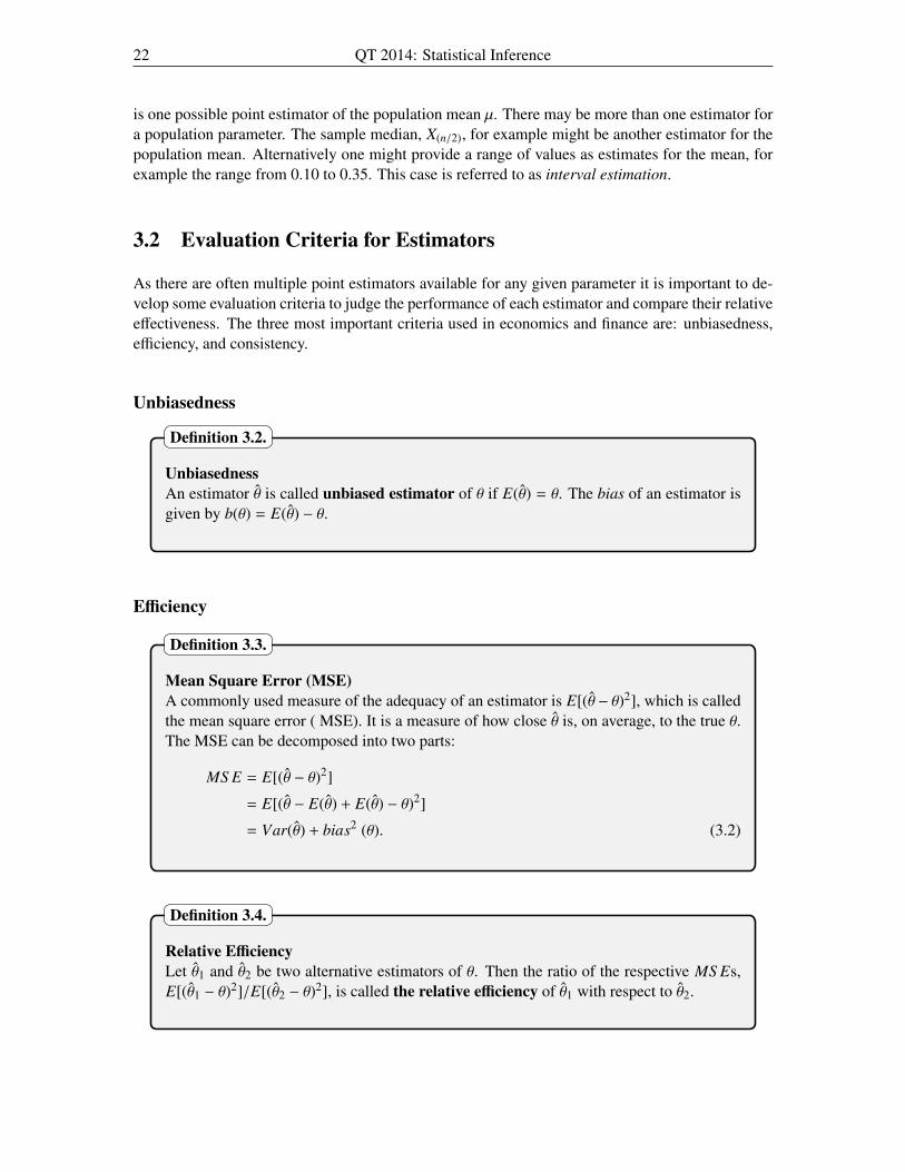
is one possible point estimator of the population mean µ. There may be more than one estimator fora population parameter. The sample median, X(n/2), for example might be another estimator for thepopulation mean. Alternatively one might provide a range of values as estimates for the mean, forexample the range from 0.10 to 0.35. This case is referred to as interval estimation.
3.2 Evaluation Criteria for Estimators
As there are often multiple point estimators available for any given parameter it is important to de-velop some evaluation criteria to judge the performance of each estimator and compare their relativeeffectiveness. The three most important criteria used in economics and finance are: unbiasedness,efficiency, and consistency.
Unbiasedness
UnbiasednessAn estimator θ is called unbiased estimator of θ if E(θ) = θ. The bias of an estimator isgiven by b(θ) = E(θ) − θ.
Definition 3.2.
Efficiency
Mean Square Error (MSE)A commonly used measure of the adequacy of an estimator is E[(θ − θ)2], which is calledthe mean square error ( MSE). It is a measure of how close θ is, on average, to the true θ.The MSE can be decomposed into two parts:
MS E = E[(θ − θ)2]
= E[(θ − E(θ) + E(θ) − θ)2]
= Var(θ) + bias2 (θ). (3.2)
Definition 3.3.
Relative EfficiencyLet θ1 and θ2 be two alternative estimators of θ. Then the ratio of the respective MS Es,E[(θ1 − θ)2]/E[(θ2 − θ)2], is called the relative efficiency of θ1 with respect to θ2.
Definition 3.4.
3. Estimation 23
Consistency
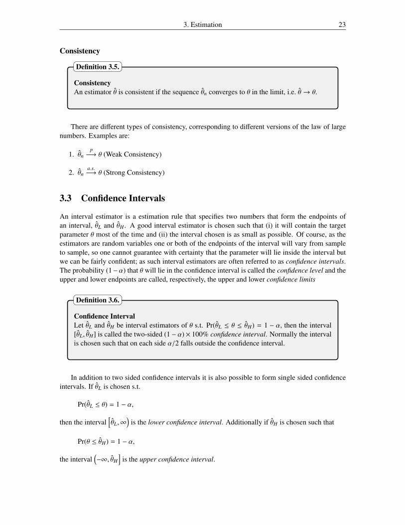
ConsistencyAn estimator θ is consistent if the sequence θn converges to θ in the limit, i.e. θ → θ.
Definition 3.5.
There are different types of consistency, corresponding to different versions of the law of largenumbers. Examples are:
1. θnp−→ θ (Weak Consistency)
2. θna.s.−→ θ (Strong Consistency)
3.3 Confidence Intervals
An interval estimator is a estimation rule that specifies two numbers that form the endpoints ofan interval, θL and θH . A good interval estimator is chosen such that (i) it will contain the targetparameter θ most of the time and (ii) the interval chosen is as small as possible. Of course, as theestimators are random variables one or both of the endpoints of the interval will vary from sampleto sample, so one cannot guarantee with certainty that the parameter will lie inside the interval butwe can be fairly confident; as such interval estimators are often referred to as confidence intervals.The probability (1−α) that θ will lie in the confidence interval is called the confidence level and theupper and lower endpoints are called, respectively, the upper and lower confidence limits
Confidence IntervalLet θL and θH be interval estimators of θ s.t. Pr(θL ≤ θ ≤ θH) = 1 − α, then the interval[θL, θH] is called the two-sided (1 − α) × 100% confidence interval. Normally the intervalis chosen such that on each side α/2 falls outside the confidence interval.
Definition 3.6.
In addition to two sided confidence intervals it is also possible to form single sided confidenceintervals. If θL is chosen s.t.
Pr(θL ≤ θ) = 1 − α,
then the interval[θL,∞
)is the lower confidence interval. Additionally if θH is chosen such that
Pr(θ ≤ θH) = 1 − α,
the interval(−∞, θH
]is the upper confidence interval.

24 QT 2014: Statistical Inference
Pivotal Method
A useful method for finding the endpoints of confidence intervals is the pivotal method, which relieson finding a pivotal quantity
Pivotal QuantityThe random variable Q = q(X1, . . . , Xn) is said to be a pivotal quantity if the distributionof Q is independent from θ.
Definition 3.7.
For example for a random sample drawn from N(µ, 1) the random variable Q =X−µ1/n is a pivotal
quantity since Q ∼ N(0, 1). For the more general case of a random sample drawn from N(µ, σ2) thepivotal quantity associated with µ will be Q =
X−µS/n , where S is the sample estimate of the standard
deviation, as Q ∼ tn−1
Pr(q1 ≤ Q ≤ q2) is unaffected by a change of scale or a translation of Q. That is if
Pr (q1 ≤ Q ≤ q2) = (1 − α) (3.3)
Pr (a + bq1 ≤ a + bQ ≤ a + bq2) = (1 − α) (3.4)
Thus, if we know the pdf of Q, it may be possible to use the operations of addition and multipli-cation to find out the desired confidence interval. Let’s take as an example a sample drawn from anormal population with known variance. To build a confidence interval around the mean the pivotalquantity of interest is
Q = X ∼ N(µ, 1/n) ∼ N(0, 1). (3.5)
To find the confidence limits µL and µH s.t.
Pr (µL ≤ µ ≤ µH) = 1 − α, (3.6)
we start with finding the confidence limits q1 and q2 of our pivotal quantity s.t.
Pr(q1 ≤
x − µ1/√
n≤ q2
)= 1 − α. (3.7)
After we have found q1 and q2, we can manipulate the probability to find expressions for µL and µH .
Pr(q1 ≤
x − µ1/√
n≤ q2
)= Pr
(1√
nq1 ≤ x − µ ≤
1√
nq2
)= Pr
(1√
nq1 − x ≤ −µ ≤
1√
nq2 − x
)= Pr
(x −
1√
nq2 ≤ µ ≤ x −
1√
nq1
). (3.8)

3. Estimation 25
So,
µL = x −1√
nq2 (3.9)
µH = x −1√
nq1 (3.10)
and [x −
1√
nq2, x −
1√
nq1
](3.11)
is the (1 − α)100% confidence interval for µ.
Constructing Confidence Intervals
Confidence Intervals for the Mean of a Normal Population
Consider the case of a sample drawn from a normal population where both µ and σ2 are unknown.We know that
Q =x − µ
S√n
∼ t(n−1). (3.12)
As the distribution of Q does not depend on any unknown parameters, Q is a pivotal quantity.We start with finding the confidence limits q1 and q2 of the pivotal quantity. As a t-distribution
is symmetrical (just like the normal distribution), we can simplify the problem somewhat as it canbe shown that q2 = −q1 = q. So we need to find a number q s.t.
Pr
−q ≤x − µ
s√n
≤ q
= 1 − α. (3.13)
which reduces to finding q s.t.
Pr (Q ≥ q) =α
2. (3.14)
After we have retrieved q = t α2 ,(n−1), we manipulate the quantities inside the probability to find
Pr(x − q
s√
n≤ µ ≤ x + q
s√
n
)= 1 − α. (3.15)
To obtain the confidence interval[x − t( α2 ,(n−1))
s√
n, x + t α
2 ,(n−1)s√
n
](3.16)
26 QT 2014: Statistical Inference
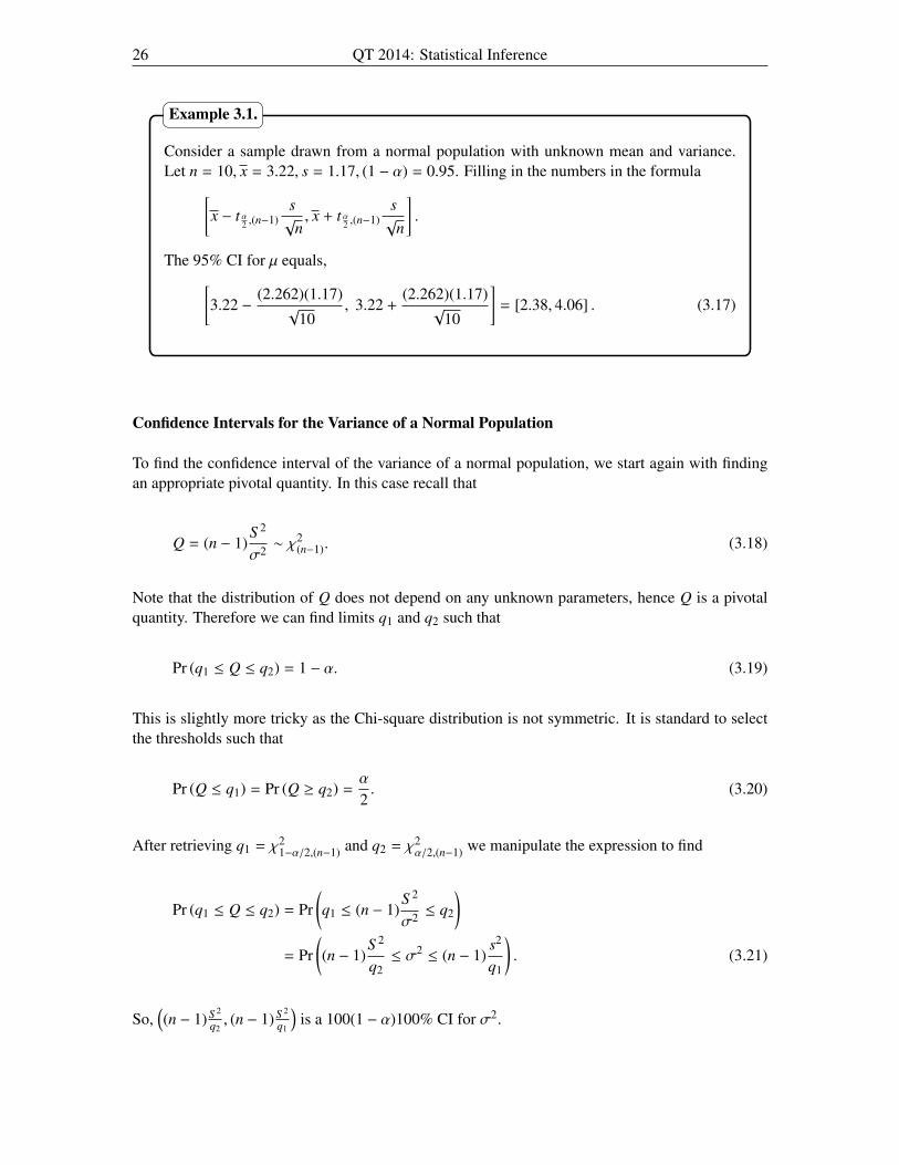
Consider a sample drawn from a normal population with unknown mean and variance.Let n = 10, x = 3.22, s = 1.17, (1 − α) = 0.95. Filling in the numbers in the formula[
x − t α2 ,(n−1)
s√
n, x + t α
2 ,(n−1)s√
n
].
The 95% CI for µ equals,[3.22 −
(2.262)(1.17)√
10, 3.22 +
(2.262)(1.17)√
10
]= [2.38, 4.06] . (3.17)
Example 3.1.
Confidence Intervals for the Variance of a Normal Population
To find the confidence interval of the variance of a normal population, we start again with findingan appropriate pivotal quantity. In this case recall that
Q = (n − 1)S 2
σ2 ∼ χ2(n−1). (3.18)
Note that the distribution of Q does not depend on any unknown parameters, hence Q is a pivotalquantity. Therefore we can find limits q1 and q2 such that
Pr (q1 ≤ Q ≤ q2) = 1 − α. (3.19)
This is slightly more tricky as the Chi-square distribution is not symmetric. It is standard to selectthe thresholds such that
Pr (Q ≤ q1) = Pr (Q ≥ q2) =α
2. (3.20)
After retrieving q1 = χ21−α/2,(n−1) and q2 = χ2
α/2,(n−1) we manipulate the expression to find
Pr (q1 ≤ Q ≤ q2) = Pr(q1 ≤ (n − 1)
S 2
σ2 ≤ q2
)= Pr
((n − 1)
S 2
q2≤ σ2 ≤ (n − 1)
s2
q1
). (3.21)
So,((n − 1) S 2
q2, (n − 1) S 2
q1
)is a 100(1 − α)100% CI for σ2.

3. Estimation 27
As in the example of the previous sample, let n = 10, x = 3.22, s = 1.17, (1 − α) = 0.95.The 95 percent CI for σ2 is[
(n − 1)s2
q2, (n − 1)
s2
q1
],
with q2 = χ20.025, (9) = 19.02 and q1 = χ2
0.975, (9) = 2.70. so the 95% CI equals[9 ×
1.172
19.02, 9 ×
1.172
2.70
]= [0.65, 4.56] . (3.22)
Example 3.2.
Problems
1. Let X1, X2, . . . , Xn be a random sample with mean µ and variance σ2. Consider the followingestimators:
(i) µ1 =X1+Xn
2
(ii) µ2 =X14 + 1
2
∑n−1i=2 Xi
(n−2) +Xn4
(iii) µ3 =∑n
i=1 Xi
n+k where 0 < k ≤ 3.
(iv) µ4 = X
(a) Explain for each estimator whether they are unbiased and/or consistent.
(b) Find the efficiency of µ4 relative to µ1, µ2, and µ3. Assume n = 36.
2. Consider the case in which two estimators are available for some parameter, θ.
Suppose that E(θ1) = E(θ2) = θ, Var(θ1) = σ21, and Var(θ2) = σ2
2.
Consider now a third estimator, θ3, defined as
θ3 = aθ1 + (1 − a)θ2.
How should a constant a be chosen in order to minimise the variance of θ3?
(a) Assume that θ1 and θ2 are independent.
(b) Assume that θ1 and θ2 are not independent but are such that Cov(θ1, θ2) = γ , 0.
3. Consider a random sample drawn from a normal population with unknown mean and variance.You have the following information about the sample: n = 21, x = 10.15, and s = 2.34. Letα = 0.10 throughout this question.
(a) Calculate the (1 − α) two-sided, upper, and lower confidence intervals for µ.
(b) Calculate the (1 − α) two-sided, upper, and lower confidence intervals for σ2.

28 QT 2014: Statistical Inference
(c) Calculate the (1 − α) two-sided, upper, and lower confidence intervals for σ.
4. Indicate for each of the following statements whether they are true, false, or uncertain. Ex-plain your answer.
(a) The center of a 95% confidence interval for the population mean is a random variable.
(b) A 95% confidence interval for µ will contain the sample mean with probability 95%.
(c) Out of one hundred 95% confidence intervals for µ, 95 will contain µ.
(d) A 95% confidence interval contains 95% of the population.

Chapter 4
Hypothesis Testing
Literature
Required Reading
• WMS, Chapter 10
Recommended Further Reading
• R, Sections 9.1 – 9.3
• CB, Chapter 8.
• G, Chapter 5.
4.1 Introduction
Think for a second about a courtroom drama. A defendant is led down the aisle, the prosecutionlays out all the evidence, and at the end the judge has to weigh the evidence and make his verdict:innocent or guilty. In many ways a legal trial follows the same logic as a statistical hypothesis test.
The testing of statistical hypotheses on unknown parameters of a probability model is one ofthe most important steps of any empirical study. Examples of statistical hypothesis that are testedin economics include
• The comparison of two alternative models,
• The evaluation of the effects of a policy change,
• The testing of the validity of an economic theory.
4.2 The Elements of a Statistical Test
Broadly speaking there are two main approaches to hypothesis testing: the classical approach andthe Bayesian approach. The approach followed in this chapter is the classical approach, which ismost widely used in econometrics. The classical approach is best described by the Neyman-Pearson
29

30 QT 2014: Statistical Inference
methodology; it can be roughly described as a decision rule that follows the logic: ‘What type ofdata will lead me to reject the hypothesis?’ A decision rule that selects one of the inferences ‘rejectthe null hypothesis’ or ‘do not reject the null hypothesis’ is called a statistical test. Any statisticaltest of hypotheses is composed of the same three essential components:
1. Selecting a null hypothesis, H0, and an alternative hypothesis, H1,
2. Choosing a test statistic,
3. Defining the rejection region.
Null and Alternative Hypotheses
A hypothesis can be thought of as a binary partition of the parameter space Θ into two sets, Θ0 andΘ1 such that
Θ0 ∩ Θ1 = � and Θ0 ∪ Θ1 = Θ. (4.1)
The set Θ0 is called the null hypothesis, denoted by H0. The set Θ1 is called the alternative hypoth-esis, denoted by H1 or Ha.
Take as example a political poll. Let’s assume that the current prime minister declares thathe has got the support of more than half the population and we do not believe him. To test hisstatement we randomly select 100 voters and ask them if they approve of the prime minister. Wecan now formulate a null and alternative hypothesis.
Let the null hypothesis be that the prime minister is correct, in that case the proportion of peoplesupporting the prime minister will be at least 0.5, so
H0 : θ ≥ 0.5. (4.2)
Conversely if the prime minister is wrong then the alternative is true
H1 : θ < 0.5. (4.3)
Note that this partitioning of the null and alternative is done such that there is no value for θ thatlies both in the domain of the null and the alternative and the union of the null and the alternativecontains all possible values that θ can take.
Often the null hypothesis in the above case is simplified: we are really only interested in theendpoint of the interval described by the null hypothesis, in this case the point θ = 0.5, so often thenull is written instead as
H0 : θ = 0.5, (4.4)
where it is implicit that any value for θ larger than 0.5 is covered by this hypothesis by the way thealternative is formulated.
The above example outlines what is known as a single sided hypothesis as the alternative hy-pothesis lies to one side of the null hypothesis. Alternatively one can specify a two sided hypothesissuch as
H0 : θ = 0.5 vs. H1 : θ , 0.5. (4.5)
In this case the alternative hypothesis includes values for θ that lie on both sides of the postulatednull hypothesis.
4. Hypothesis Testing 31
Test Statistic
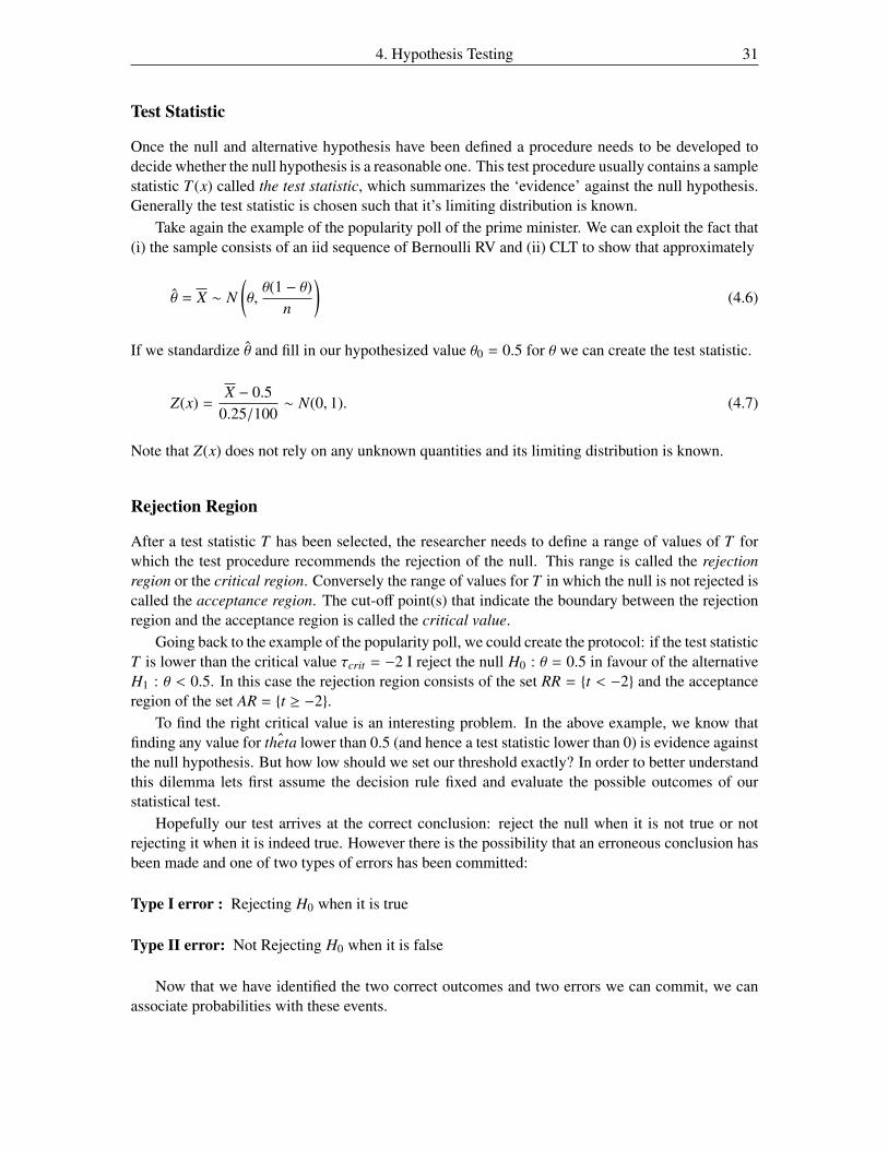
Once the null and alternative hypothesis have been defined a procedure needs to be developed todecide whether the null hypothesis is a reasonable one. This test procedure usually contains a samplestatistic T (x) called the test statistic, which summarizes the ‘evidence’ against the null hypothesis.Generally the test statistic is chosen such that it’s limiting distribution is known.
Take again the example of the popularity poll of the prime minister. We can exploit the fact that(i) the sample consists of an iid sequence of Bernoulli RV and (ii) CLT to show that approximately
θ = X ∼ N(θ,θ(1 − θ)
n
)(4.6)
If we standardize θ and fill in our hypothesized value θ0 = 0.5 for θ we can create the test statistic.
Z(x) =X − 0.5
0.25/100∼ N(0, 1). (4.7)
Note that Z(x) does not rely on any unknown quantities and its limiting distribution is known.
Rejection Region
After a test statistic T has been selected, the researcher needs to define a range of values of T forwhich the test procedure recommends the rejection of the null. This range is called the rejectionregion or the critical region. Conversely the range of values for T in which the null is not rejected iscalled the acceptance region. The cut-off point(s) that indicate the boundary between the rejectionregion and the acceptance region is called the critical value.
Going back to the example of the popularity poll, we could create the protocol: if the test statisticT is lower than the critical value τcrit = −2 I reject the null H0 : θ = 0.5 in favour of the alternativeH1 : θ < 0.5. In this case the rejection region consists of the set RR = {t < −2} and the acceptanceregion of the set AR = {t ≥ −2}.
To find the right critical value is an interesting problem. In the above example, we know thatfinding any value for ˆtheta lower than 0.5 (and hence a test statistic lower than 0) is evidence againstthe null hypothesis. But how low should we set our threshold exactly? In order to better understandthis dilemma lets first assume the decision rule fixed and evaluate the possible outcomes of ourstatistical test.
Hopefully our test arrives at the correct conclusion: reject the null when it is not true or notrejecting it when it is indeed true. However there is the possibility that an erroneous conclusion hasbeen made and one of two types of errors has been committed:
Type I error : Rejecting H0 when it is true
Type II error: Not Rejecting H0 when it is false
Now that we have identified the two correct outcomes and two errors we can commit, we canassociate probabilities with these events.

32 QT 2014: Statistical Inference
Table 4.1: Decision outcomes and their associated probabilities
H0 rejected H0 not rejected
H0 true α (1 − α)Type I errorLevel / Size
H0 false (1 − β) β
Type II errorPower Operating Char.
Size of the test(α)The probability of rejecting H0 when it is actually true (ie. committing a type I error) iscalled the size of the test. Sometimes it is also called the level of significance of the test.This probability is usually denoted as α.Common sizes that are used in hypothesis testing are α = 0.10, α = 0.05, and α = 0.01.
Definition 4.1.
Power of the test (1 − β)The probability of rejecting H0 when it is false is called the power of the test. Thisprobability is normally denoted as (1 − β).
Definition 4.2.
Operating Characteristic (β)The probability of not rejecting H0 when it is actually false (ie. committing a type II error)is known as the operating characteristic. This probability is usually denoted as β. Thisconcept is widely used in statistical quality control theory.
Definition 4.3.
Table 4.2 below summarizes the probabilities. Ideally a test is chosen such that both the prob-ability of a type I error,α, and the probability of a type II error,β, are as low as possible.However,practically this is impossible because, given some fixed sample, reducing α increases β: there isa trade-off between the two. The only way to decrease both α and β is to increase the samplesize, something that is often not feasible. The classical decision procedure therefore chooses anacceptable value for the level α.
Note that in small samples the empirical size associated with a critical value of a test statistic isoften larger than the asymptotic size because the approximation of the limiting distribution might
4. Hypothesis Testing 33
not yet be very good. Thus if a researcher is not careful he risks choosing a test which rejects thenull hypothesis more often than he realizes.
So then how do we select the critical value τcrit after fixing α? Let’s consider once more ourpopularity contest. Recall that the test statistic associated with the hypothesis that θ = 0.5 was(X − 0.5)/(0.25/100) ∼ N(0, 1). Let’s say that we are willing to reject the null hypothesis if there isless than 2.5% probability of committing a type I error, ie. α = 0.025. Since we know the limitingdistribution of T we can find the value τcrit such that
Pr[T < τcrit | θ = 0.5] = α = 0.025. (4.8)
This value can be found by looking up the CDF of a standard normal: Pr(T ≥ τ) = 1−0.025 = 0.975;in this case τ = −1.96. In any case, we have now found the relevant critical value, and can definethe rejection region as RR = {t < −1.96} and the acceptance region as AR = {t ≥ −1.96}. If we mapthe critical value of the test statistic back to a proportion, this translates to θcrit = θ − 1.96 × se =
0.5 − 1.96 × 0.05 = 0.402; ie. we can reject the null (θ = 0.5) at the 2.5% level if we find a samplemean lower than 0.402.
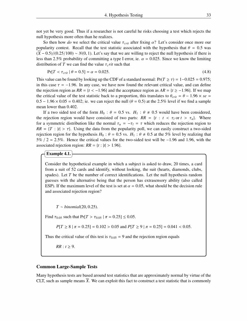
If a two sided test of the form H0 : θ = 0.5 vs. H1 : θ , 0.5 would have been considered,the rejection region would have consisted of two parts: RR = {t : t < τl or t > τu}. Wherefor a symmetric distribution like the normal τu = −τl = τ which reduces the rejection region toRR = {T : |t| > τ}. Using the data from the popularity poll, we can easily construct a two-sidedrejection region for the hypothesis H0 : θ = 0.5 vs. H1 : θ , 0.5 at the 5% level by realizing that5% / 2 = 2.5%. Hence the critical values for the two-sided test will be −1.96 and 1.96, with theassociated rejection region: RR = {t : |t| > 1.96}.
Consider the hypothetical example in which a subject is asked to draw, 20 times, a cardfrom a suit of 52 cards and identify, without looking, the suit (hearts, diamonds, clubs,spades). Let T be the number of correct identifications. Let the null hypothesis randomguesses with the alternative being that the person has extrasensory ability (also calledESP). If the maximum level of the test is set at α = 0.05, what should be the decision ruleand associated rejection region?
T ∼ binomial(20, 0.25).
Find τ0.05 such that Pr[T > τ0.05 | π = 0.25] ≤ 0.05.
P[T ≥ 8 | π = 0.25] = 0.102 > 0.05 and P[T ≥ 9 | π = 0.25] = 0.041 < 0.05.
Thus the critical value of this test is τ0.05 = 9 and the rejection region equals
RR : t ≥ 9.
Example 4.1.
Common Large-Sample Tests
Many hypothesis tests are based around test statistics that are approximately normal by virtue of theCLT, such as sample means X. We can exploit this fact to construct a test statistic that is commonly

34 QT 2014: Statistical Inference
encountered in econometrics.
Z =θ − θ0
σθ∼ N(0, 1). (4.9)
The standard error is often replaced with its sample estimate S/n which results in the following teststatistic
T =θ − θ0
S/n∼ t(n−1). (4.10)
with associated two-sided rejection region
RR : {t : |t| > τα/2} or RR : {θ : θ < θ − τα/2σθ or θ > θ + τα/2σθ}. (4.11)
4.3 Duality of Hypothesis Testing and Confidence Intervals
Recall the concept of a (1 − α) two-sided confidence interval[θl, θh
]as an interval that contains
the true parameter θ with probability (1 − α). Also recall that if the sampling distribution of θ isapproximately normal then the (1 − α) confidence interval is given by
θ ± zα/2σθ, (4.12)
with σθ the standard error of the estimator and zα/2 the value such that Pr(Z > zα/2) = α/2.Note the strong similarity with this confidence interval and the test statistic plus associated
rejection region of a two sided hypothesis test described in the previous section. This is no coin-cidence. Consider again the two-sided rejection region for a test with level α from the previoussection: RR : {z : |z| > zα/2}. The complement of the rejection region, RR, is the acceptance regionAR : {z : |z| ≤ zα/2} which maps onto the parameter space as do not reject (‘accept’) null hypothesisat level α if the estimate lies in the interval
θ0 ± zα/2σθ. (4.13)
Restated, for all θ0 that lie in the interval
θ − zα/2σθ ≥ θ0 ≥ θ + zα/2σθ. (4.14)
the estimate θ will lie inside the acceptance region and the null hypothesis cannot be rejected atlevel α. This interval is, as you will notice, exactly equal to the (1 − α) confidence interval outlinedabove. Thus the duality between confidence intervals and hypothesis testing: if the hypothesizedvalue θ0 lies inside the (1− α) confidence interval, one cannot reject the null hypothesis H0 : θ = θ0vs. H1 : θ , θ0 at level α; if θ0 does not lie in the confidence interval then the null can be rejectedat level α. A similar statement can be made for upper and lower single sided confidence intervals.
Notice that any value inside the confidence interval would be an ‘acceptable’ value for the nullhypothesis, in the sense that it cannot be rejected with a hypothesis test of level α. This explainswhy in statistics we usually only talk about rejecting the null vs. not rejecting the null, rather thansaying we ‘accept’ the null. Even if we do not reject the null we recognize that there are probablymany other values for θ that would be acceptable and we should be hesitant to make statementsabout a single θ being the single true value. Likewise we do not commonly ‘accept’ the alternativewhen we reject the null hypothesis are there are usually many potential values the paramater θ cantake under the alternative.

4. Hypothesis Testing 35
4.4 Attained Significance Levels: P-Values
Recall that the most common method of selecting a critical value for the test statistic and deter-mining the rejection region is fixing the level of the test α. Of course we would like to have α assmall as possible as it denotes the probability of committing a type I error. However, as discussed,choosing a low α comes at the cost of increasing β, the probability of a type II error. Choosing thecorrect value of α is thus important, but also rather arbitrary. While one researcher would be happyto conduct a test with level α = 0.10 another would insist upon only testing with levels lower than,say, α = 0.05. Furthermore, the levels of tests are often fixed at 10%, 5%, or 1% not as a result oflong deliberations, but rather out of custom and tradition.
There is a way to partially sidestep this issue of selecting the right value for α by reportingthe attained significance level or p-value. For example let T be a test statistic for the hypothesisH0 : θ = θ0 vs. H1 : θ > θ0. If the realized value of the test statistic is t, based on our sample, thenthe p-value is calculated as the probability
pval = Pr[T > t | θ0]. (4.15)
p-value The attained significance level, or p-value, is the smallest level of significance αat which the null hypothesis can be reject given the observed sample.
Definition 4.4.
The advantage of reporting a p-value, rather than fixing the level of the test yourself is that itpermits each of your readers to draw their own conclusion about the strength of your results. Theprocedures for finding p-values are very similar to those of finding the critical value of a test statistic.However, instead of fixing the probability α and finding the critical value of the test statistic τ, wenow fix the value of the test statistic t and find the associated probability pval.
A financial analyst believes that firms experience positive stock returns upon the an-nouncement that they are targeted for a takeover. To test his hypothesis he has collecteda data set comprising 300 take-over announcements with an average abnormal return ofr = 1.5% on the announcement date, with a standard error of 0.5%. Calculate the p-valueof the null hypothesis H0 : r = 0 vs. H0 : r > 0.Invoking CLT, the natural test statistic to test this hypothesis is
Z =rabn − 0
S rabn
∼ t(99) ≈ N(0, 1).
The value of the test statistic in this sample equals z = 1.5/0.5 = 3. Looking up the value3 in the standard normal table yields us p-val = Pr[Z > 3] = 0.0013. Thus the p-value ofthis test is 0.13%, implying that we can easily reject the null hypothesis of no news effectat the 10%, 5%, or 1% level.
Example 4.2.

36 QT 2014: Statistical Inference
4.5 Power of the Test
In the previous sections we have primarily focused on the probability α of committing a type I error.However, it is at least as important for a test to also have a low probability β of committing a typeII error. Remember that a type II error is committed if the testing procedure fails to reject the nullwhen it was in fact false. In econometrics, rather than looking directly at β, many statistical testsare evaluated by its complement (1− β): the probability that a statistical test rejects the null when itis indeed false; this probability (1 − β) is called the power of the test.
Before we can calculate the power of a test there are two issues that need to be addressed.Firstly, recall that the alternative hypothesis often contains a large range of potential values for θ.For instance in the single sided hypothesis H0 : θ = θ0 vs H1 : θ > θ0, all values of θ larger thanθ0 are included in the alternative. However, the power will normally not be the same for all thesedifferent values included in Θ1. Therefore the power of a test is often evaluated at specific valuesfor the alternative, say θ = θ1.
Secondly, as we have focused on type I errors and the associated α’s, we have only consideredhow the sampling distribution looks like under the assumption that the null hypothesis is correct.This sampling distribution is referred to as the null distribution. However, if we are interested aboutmaking statements about the power of the test (or type II errors), then we have to consider how thesampling distribution of θ looks like when θ = θ1. That is, we evaluate the sampling distribution forthat specific alternative.
Consider once more the one-sided hypothesis H0 : θ = θ0 vs. H0 : θ > θ0 with the associatedtest statistic T and critical value τα. For a specific alternative θ = θ1 (with θ1 > θ0) the power of thetest can be calculated as the conditional probability
(1 − β) = Pr[T > τ | θ = θ1]. (4.16)
Note that the main difference with the definition of α
α = Pr[T > τ | θ = θ0], (4.17)
is that the probability is conditioned on the alternative hypothesis being true, rather than the as-sumption that the null hypothesis is true.
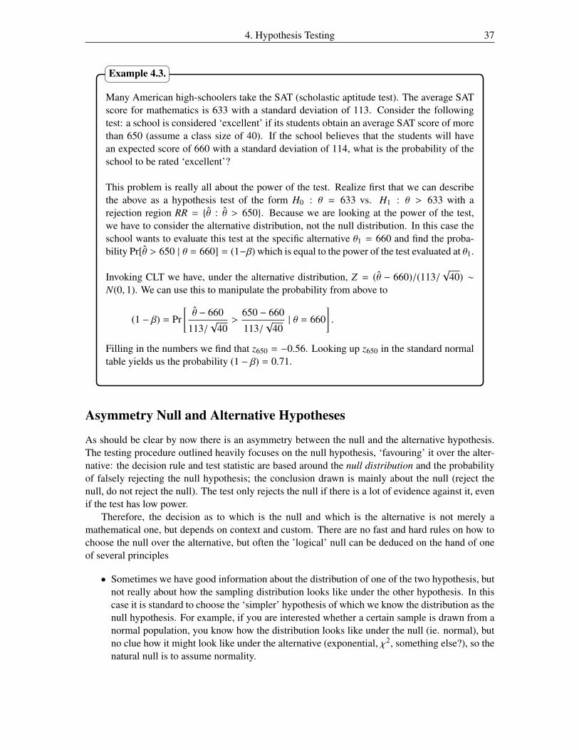
4. Hypothesis Testing 37
Many American high-schoolers take the SAT (scholastic aptitude test). The average SATscore for mathematics is 633 with a standard deviation of 113. Consider the followingtest: a school is considered ‘excellent’ if its students obtain an average SAT score of morethan 650 (assume a class size of 40). If the school believes that the students will havean expected score of 660 with a standard deviation of 114, what is the probability of theschool to be rated ‘excellent’?
This problem is really all about the power of the test. Realize first that we can describethe above as a hypothesis test of the form H0 : θ = 633 vs. H1 : θ > 633 with arejection region RR = {θ : θ > 650}. Because we are looking at the power of the test,we have to consider the alternative distribution, not the null distribution. In this case theschool wants to evaluate this test at the specific alternative θ1 = 660 and find the proba-bility Pr[θ > 650 | θ = 660] = (1−β) which is equal to the power of the test evaluated at θ1.
Invoking CLT we have, under the alternative distribution, Z = (θ − 660)/(113/√
40) ∼N(0, 1). We can use this to manipulate the probability from above to
(1 − β) = Pr[θ − 660
113/√
40>
650 − 660
113/√
40| θ = 660
].
Filling in the numbers we find that z650 = −0.56. Looking up z650 in the standard normaltable yields us the probability (1 − β) = 0.71.
Example 4.3.
Asymmetry Null and Alternative Hypotheses
As should be clear by now there is an asymmetry between the null and the alternative hypothesis.The testing procedure outlined heavily focuses on the null hypothesis, ‘favouring’ it over the alter-native: the decision rule and test statistic are based around the null distribution and the probabilityof falsely rejecting the null hypothesis; the conclusion drawn is mainly about the null (reject thenull, do not reject the null). The test only rejects the null if there is a lot of evidence against it, evenif the test has low power.
Therefore, the decision as to which is the null and which is the alternative is not merely amathematical one, but depends on context and custom. There are no fast and hard rules on how tochoose the null over the alternative, but often the ’logical’ null can be deduced on the hand of oneof several principles
• Sometimes we have good information about the distribution of one of the two hypothesis, butnot really about how the sampling distribution looks like under the other hypothesis. In thiscase it is standard to choose the ‘simpler’ hypothesis of which we know the distribution as thenull hypothesis. For example, if you are interested whether a certain sample is drawn from anormal population, you know how the distribution looks like under the null (ie. normal), butno clue how it might look like under the alternative (exponential, χ2, something else?), so thenatural null is to assume normality.
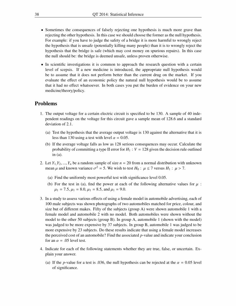
38 QT 2014: Statistical Inference
• Sometimes the consequences of falsely rejecting one hypothesis is much more grave thanrejecting the other hypothesis. In this case we should choose the former as the null hypothesis.For example: if you have to judge the safety of a bridge it is more harmful to wrongly rejectthe hypothesis that is unsafe (potentially killing many people) than it is to wrongly reject thehypothesis that the bridge is safe (which may cost money on spurious repairs). In this casethe null should be: the bridge is deemed unsafe, unless proven otherwise.
• In scientific investigations it is common to approach the research question with a certainlevel of scepsis. If a new medicine is introduced, the appropriate null hypothesis wouldbe to assume that it does not perform better than the current drug on the market. If youevaluate the effect of an economic policy the natural null hypothesis would be to assumethat it had no effect whatsoever. In both cases you put the burden of evidence on your newmedicine/theory/policy.
Problems
1. The output voltage for a certain electric circuit is specified to be 130. A sample of 40 inde-pendent readings on the voltage for this circuit gave a sample mean of 128.6 and a standarddeviation of 2.1.
(a) Test the hypothesis that the average output voltage is 130 against the alternative that it isless than 130 using a test with level α = 0.05.
(b) If the average voltage falls as low as 128 serious consequences may occur. Calculate theprobability of committing a type II error for H1 : V = 128 given the decision rule outlinedin (a).
2. Let Y1,Y2, ...,Yn be a random sample of size n = 20 from a normal distribution with unknownmean µ and known variance σ2 = 5. We wish to test H0 : µ ≤ 7 versus H1 : µ > 7.
(a) Find the uniformly most powerful test with significance level 0.05.
(b) For the test in (a), find the power at each of the following alternative values for µ :µ1 = 7.5, µ1 = 8.0, µ1 = 8.5, and µ1 = 9.0.
3. In a study to assess various effects of using a female model in automobile advertising, each of100 male subjects was shown photographs of two automobiles matched for price, colour, andsize but of different makes. Fifty of the subjects (group A) were shown automobile 1 with afemale model and automobile 2 with no model. Both automobiles were shown without themodel to the other 50 subjects (group B). In group A, automobile 1 (shown with the model)was judged to be more expensive by 37 subjects. In group B, automobile 1 was judged to bemore expensive by 23 subjects. Do these results indicate that using a female model increasesthe perceived cost of an automobile? Find the associated p-value and indicate your conclusionfor an α = .05 level test.
4. Indicate for each of the following statements whether they are true, false, or uncertain. Ex-plain your answer.
(a) If the p-value for a test is .036, the null hypothesis can be rejected at the α = 0.05 levelof significance.

4. Hypothesis Testing 39
(b) In a formal test of hypothesis, α is the probability that the null hypothesis is incorrect.
(c) If the a test is rejected at the significance level α, it will also always be rejected at signif-icance level 2 × α
(d) If the level of a test is decreased, the power would be expected to increase.
tab1

40 QT 2014: Statistical Inference

Appendix A
Exercise Solutions
A.1 Sampling Distributions
1. (a)
E(X) = µ1,
Var(X) = n−1σ21.
(b)
E(X − Y) = 0,
Var(X) = n−1σ21 + m−1σ2
2
= n−1(σ21 + σ2
2)
= 4.5/n.
(c)
σX−Y = 0.1√
4.5/√
n = 0.1
n = 4.5/(0.1)2
n = 450.
2. (a)∑4 Zi ∼ N(0, 4)
(b)∑4 Z2
i ∼ χ24
(c) Z21/
∑4i=2 Zi ∼ F1,3
(d) Z1/√∑4
i=2 Z2i /3 ∼ t3
3. (a) F. Like the standard error, this is a fixed number (σ2/n). The estimated variance, ofcourse, is a random variable.
(b) T. S E = σ/√
n. For every quadrupling of the sample size, the S E halves.(c) F. Inference on a random sample is easiest, but inference can alo be obtained using
independent, or even dependent samples, as long as due care is taken.(d) T. If T is t(n), then T 2 will be F(n, 1).
41
42 QT 2014: Statistical Inference
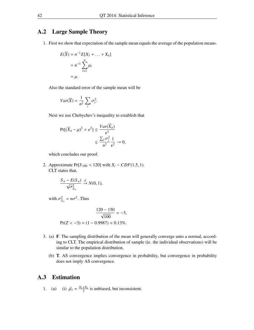
A.2 Large Sample Theory
1. First we show that expectation of the sample mean equals the average of the population means.
E(X) = n−1E[X1 + . . . + Xn]
= n−1n∑
i=1
µi
= µ.
Also the standard error of the sample mean will be
Var(X) =1n2
∑i
σ2i .
Next we use Chebychev’s inequality to establish that
Pr[(Xn − µ)2 > ε2] ≤Var(Xn)
ε2
≤
∑i σ
2i
n2
1ε2 → 0,
which concludes our proof.
2. Approximate Pr[S 100 < 120] with Xi ∼ CDF(1.5, 1).CLT states that,
S n − E(S n)√σ2
S n
d→ N(0, 1),
with σ2S n
= nσ2. Thus
120 − 150√
100= −3,
Pr(Z < −3) = (1 − 0.9987) ≈ 0.13%.
3. (a) F. The sampling distribution of the mean will generally converge unto a normal, accord-ing to CLT. The empirical distribution of sample (ie. the individual observations) will besimilar to the population distribution.
(b) T. AS convergence implies convergence in probability, but convergence in probabilitydoes not imply AS convergence.
A.3 Estimation
1. (a) (i) µ1 =X1+Xn
2 is unbiased, but inconsistent.
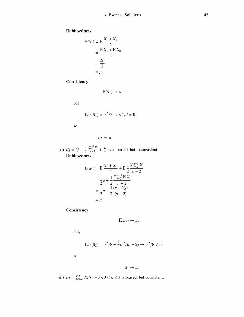
A. Exercise Solutions 43
Unbiasedness:
E[µ1] = EX1 + Xn
2
=E X1 + E Xn
2
=2µ2
= µ.
Consistency:
E(µ1)→ µ,
but
Var(µ1) = σ2/2→ σ2/2 , 0.
so
µ2 9 µ.
(ii) µ2 =X14 + 1
2
∑n−1i=2 Xi
n−2 +Xn4 is unbiased, but inconsistent.
Unbiasedness:
E(µ2) = EX1 + Xn
4+ E
12
∑n−1i=2 Xi
n − 2
=12µ +
12
∑n−1i=2 E Xi
n − 2
=12µ +
12
(n − 2)µ(n − 2)
= µ.
Consistency:
E(µ2)→ µ,
but,
Var(µ2) = σ2/8 +14σ2/(n − 2)→ σ2/8 , 0.
so
µ2 9 µ.
(iii) µ3 =∑n
i=1 Xi/(n + k), 0 < k ≤ 3 is biased, but consistent.

44 QT 2014: Statistical Inference
Unbiasedness:
E(µ3) = E((n + k)−1n∑
i=1
Xi)
= (n + k)−1n∑
i=1
E(Xi)
= (n + k)−1n∑
i=1
µ
=n
n + kµ
= µ −k
n + kµ
, µ.
Consistency:
limn→∞
[E(µ3)] = limn→∞
[n
n + kµ],
= µ.
and
Var(µ3) = n/(n + k)2σ2 → 0.
so
µ3 → µ.
(iv) µ4 = X is both unbiased and consistent, see lecture notes.
(b) Relative Efficiency: (MS E1/MS E2), with MS Ei = Var(µi) + bias2(µi). For n =
36, σ2 = 20, µ = 15, and k = 3 we have
(i) MS E1 = σ2/2 = 10(ii) MS E2 = σ2/8 + 1
4σ2/(n − 2) = 45/17
(iii) MS E3 = (n/(n + k)2σ2) + (k/(n + k)µ)2 = 80/169 + 225/169 = 300/169(iv) MS E4 = σ2/n = 20/36
So the relative efficiency of the sample mean (µ4) will be
(i) MS E4/MS E1 = 0.056(ii) MS E4/MS E2 = 0.210
(iii) MS E4/MS E3 = 0.313
2. Note that θ3 is unbiased:
E(θ3) = E(aθ1 + (1 − a)θ2)
E(θ3) = aθ + (1 − a)θ
E(θ3) = θ.
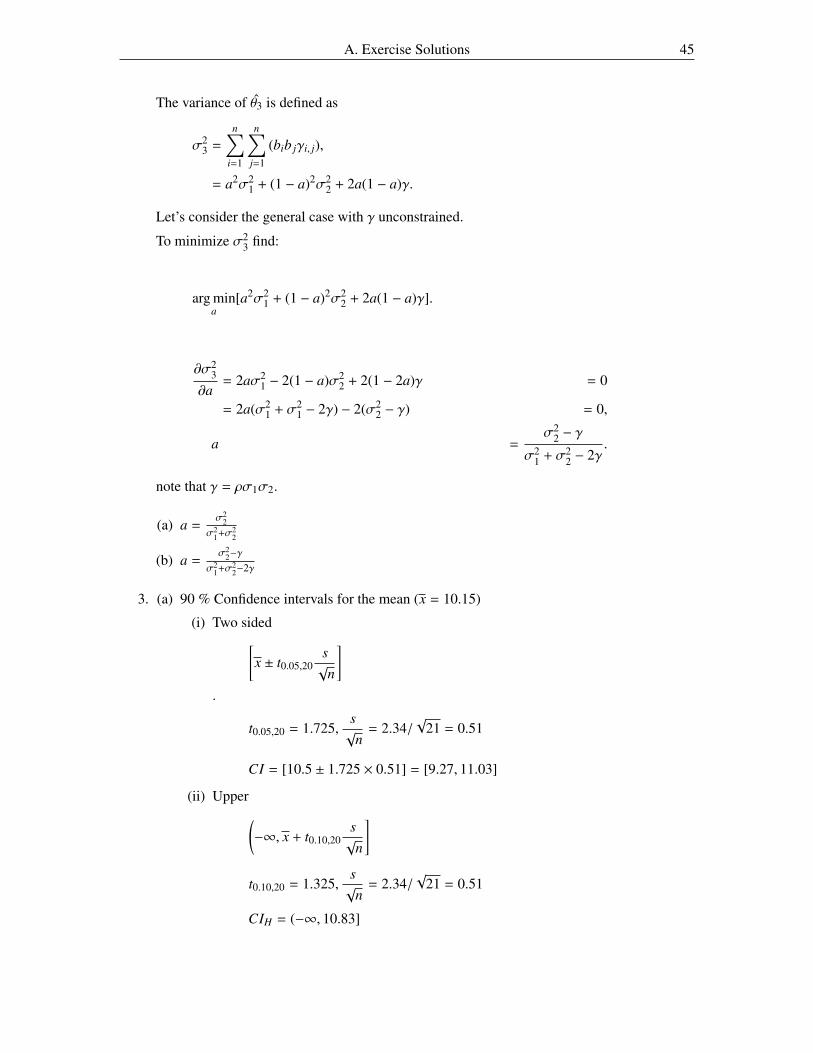
A. Exercise Solutions 45
The variance of θ3 is defined as
σ23 =
n∑i=1
n∑j=1
(bib jγi, j),
= a2σ21 + (1 − a)2σ2
2 + 2a(1 − a)γ.
Let’s consider the general case with γ unconstrained.
To minimize σ23 find:
arg mina
[a2σ21 + (1 − a)2σ2
2 + 2a(1 − a)γ].
∂σ23
∂a= 2aσ2
1 − 2(1 − a)σ22 + 2(1 − 2a)γ = 0
= 2a(σ21 + σ2
1 − 2γ) − 2(σ22 − γ) = 0,
a =σ2
2 − γ
σ21 + σ2
2 − 2γ.
note that γ = ρσ1σ2.
(a) a =σ2
2σ2
1+σ22
(b) a =σ2
2−γ
σ21+σ2
2−2γ
3. (a) 90 % Confidence intervals for the mean (x = 10.15)
(i) Two sided[x ± t0.05,20
s√
n
].
t0.05,20 = 1.725,s√
n= 2.34/
√21 = 0.51
CI = [10.5 ± 1.725 × 0.51] = [9.27, 11.03]
(ii) Upper(−∞, x + t0.10,20
s√
n
]
t0.10,20 = 1.325,s√
n= 2.34/
√21 = 0.51
CIH = (−∞, 10.83]

46 QT 2014: Statistical Inference
(iii) Lower[x − t0.10,20
s√
n,∞
)t0.10,20 = 1.325,
s√
n= 2.34/
√21 = 0.51
CIL = [9.47,∞)
(b) 90 % Confidence intervals for the variance (s2 = 2.342 = 5.48)
(i) Two sided
χ20.05,20 = 31.41; χ2
0.95,20 = 10.85
CI =
[20 × 5.48
31.41,
20 × 5.4810.85
]= [3.49, 10.10]
(ii) Upper
χ20.90,20 = 12.44
CIH = [0, 8.80]
(iii) Lower
χ20.10,20 = 28.41
CIL = [2.71,∞)
4. (a) T. Sample mean = RV.
(b) F. The CI will always contain the sample mean as it is normally centered around it.
(c) F. in expectation 95, but the actual number is a random variable
(d) F. will probably contain much less that 95% of the sample space. Aim is not to coversample space but to construct an interval capturing the parameter.
A.4 Hypothesis Testing
1. Test H0 : ν ≥ 130 vs. H1 : ν < 130 with α = 0.05. n = 40, ν = 128.6, σ = 2.1Using CLT we can construct a test statistic with known sampling statistic:
z =ν − ν
σ/√
n∼ N(0, 1),
t =ν − ν
S/√
n∼ t(n − 1),
tν =128.6 − 130
2.1/√
40=−1.40.33
= −4.24.
Rejection Region: tν < t0.05, t0.05(39) ≈ t0.05(40) = −1.684 (compare z0.05 = −1.645)
−4.24 < −1.684⇒ Reject H0 : ν is significantly lower than 130 at the 5% level.

A. Exercise Solutions 47
2. Consider H0 : µ ≤ 7 vs. Ha : µ > 7. Yi ∼ N(µ, 5), n = 20
(a) Uniformly most powerful test:
arg maxmcrit
[P(µ > mcrit | µ1)] s.t. P(µ > mcrit | µ0) ≤ α.
i.e. set mcrit s.t.
P(µ > mcrit | µ0) = 0.05.
By CLT we know that:
µ − µ
σ/√
n∼ N(0, 1),Z0.95 = 1.645.
Thus:
mcrit − µ
σ/√
n= Z0.95,
mcrit − 7√
5/20= 1.645,
mcrit = 7 + 1.645√
5/20,
= 7.8225.
i.e. rejection region: reject if µ > 7.8225.
(b) Find the power of the test:
(1 − β) = P(µ > mcrit | µ1),
When the alternative takes on the following values (Again, use CLT for the samplingdistribution):
µ1 = 7.5, (7.8225 − 7.5)/0.5 = 0.645 , (1 − β) = 0.26.
µ1 = 8.0, (7.8225 − 8.0)/0.5 = −0.335 , (1 − β) = 0.63.
µ1 = 8.5, (7.8225 − 8.5)/0.5 = −1.335 , (1 − β) = 0.91.
µ1 = 9.0, (7.8225 − 9.0)/0.5 = −2.355 , (1 − β) = 0.99.
3. In effect there are two random samples which are both a sequence of Bernoulli trails, eachwith n = 50 and some parameter φ ∈ [0, 1]. Setting up the null and alternative hypothesisyields:
H0 : φ1 ≤ φ2,H1 : φ1 > φ2
or alternatively
H0 : (φ1 − φ2) ≤ 0,H1 : (φ1 − φ2) > 0
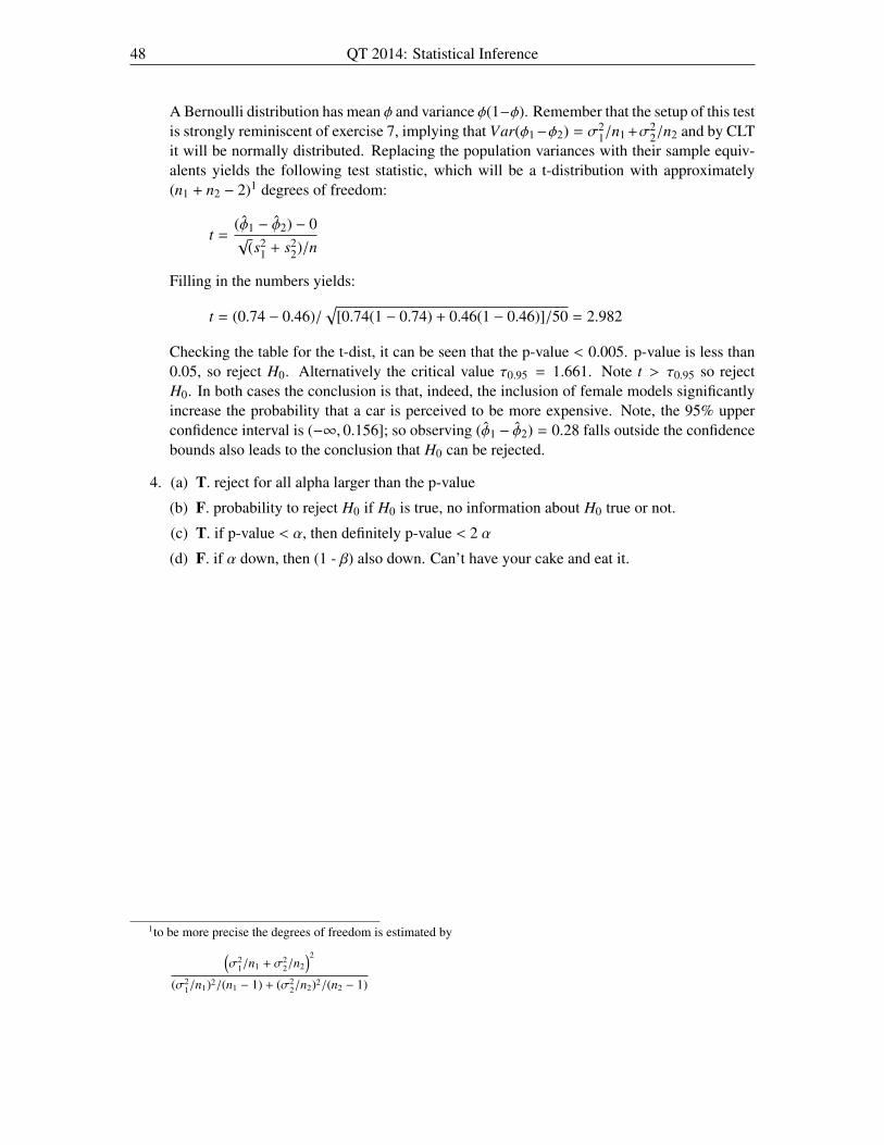
48 QT 2014: Statistical Inference
A Bernoulli distribution has mean φ and variance φ(1−φ). Remember that the setup of this testis strongly reminiscent of exercise 7, implying that Var(φ1−φ2) = σ2
1/n1 +σ22/n2 and by CLT
it will be normally distributed. Replacing the population variances with their sample equiv-alents yields the following test statistic, which will be a t-distribution with approximately(n1 + n2 − 2)1 degrees of freedom:
t =(φ1 − φ2) − 0√
(s21 + s2
2)/n
Filling in the numbers yields:
t = (0.74 − 0.46)/√
[0.74(1 − 0.74) + 0.46(1 − 0.46)]/50 = 2.982
Checking the table for the t-dist, it can be seen that the p-value < 0.005. p-value is less than0.05, so reject H0. Alternatively the critical value τ0.95 = 1.661. Note t > τ0.95 so rejectH0. In both cases the conclusion is that, indeed, the inclusion of female models significantlyincrease the probability that a car is perceived to be more expensive. Note, the 95% upperconfidence interval is (−∞, 0.156]; so observing (φ1 − φ2) = 0.28 falls outside the confidencebounds also leads to the conclusion that H0 can be rejected.
4. (a) T. reject for all alpha larger than the p-value
(b) F. probability to reject H0 if H0 is true, no information about H0 true or not.
(c) T. if p-value < α, then definitely p-value < 2 α
(d) F. if α down, then (1 - β) also down. Can’t have your cake and eat it.
1to be more precise the degrees of freedom is estimated by(σ2
1/n1 + σ22/n2
)2
(σ21/n1)2/(n1 − 1) + (σ2
2/n2)2/(n2 − 1)