1

Msc in Finance and International Business

Author: Luis Miguel Santos Neto

Student ID: ln89263

Supervisor: Baran Siyahhan

Behavioural Finance or Classical Finance? An Investigation of

Equity Risk Premium and Size Premium in an International

Context

Aarhus School of Business, Aarhus University

December 2012

2

Contents

Abstract ..................................................................................................................................... 4

Introduction .............................................................................................................................. 6

I - Is the investor rational? ........................................................................................................ 8

Introduction ........................................................................................................................... 8

Heuristics and Biases ............................................................................................................ 8

Conclusion ........................................................................................................................... 12

II - Are the Markets efficient? ................................................................................................. 13

Previous evidence ................................................................................................................ 13

Introduction ......................................................................................................................... 15

Twin shares – an example from Royal Dutch and Shell ..................................................... 19

Index inclusions and exclusions .......................................................................................... 20

Speculative Bubbles ............................................................................................................ 22

Conclusion ........................................................................................................................... 26

III - Prospect and Ambiguity Theories ..................................................................................... 27

Prospect Theory................................................................................................................... 27

Ambiguity aversion ............................................................................................................. 30

IV - MPT theory and its fundamental assumptions ................................................................. 32

V - Models derived from MPT – CAPM, Arbitrage pricing theory ........................................... 35

CAPM ................................................................................................................................. 36

Arbitrage pricing theory ...................................................................................................... 38

VI - Limitations and Criticisms ................................................................................................. 39

Modern Portfolio Theory .................................................................................................... 39

CAPM and Arbitrage Pricing Theory ................................................................................. 41

VII - Constructing a “Behavioural Portfolio” ........................................................................... 42

VIII - Combining MPT and BT in order to find the “ideal” portfolio ........................................ 45

IX - Equity premium puzzle...................................................................................................... 47

Introduction ......................................................................................................................... 47

Data Description .................................................................................................................. 47

Hypothesis ........................................................................................................................... 48

Results ................................................................................................................................. 49

Behavioural Finance explanations ...................................................................................... 51

X - Size Premium Puzzle .......................................................................................................... 55

3

Introduction ......................................................................................................................... 55

Data Description .................................................................................................................. 56

Hypothesis ........................................................................................................................... 56

Results ................................................................................................................................. 56

Behavioural Finance Explanations ...................................................................................... 60

Conclusion ............................................................................................................................... 63

Bibliography ............................................................................................................................ 64

4

Abstract

The traditional paradigm of finance has been an important paradigm through the last

decades and has some remarkable achievements in explaining market trends and finance

in general. Nevertheless, mainly through the last years some voices have criticized the

bases and foundations of some of the most important financial theories.

Behavioural finance, a way more recent approach has in the other hand grown

exponential in terms of importance and supporters in the same period.

Supporters of this new paradigm claim that Behavioural Finance, which uses new

factors (such human behaviour) on its assessment is capable to account for market

inefficiencies and other phenomena which the traditional paradigm fails to explain.

Behavioural finance goes therefore against some of the most important premises and

cornerstones of the traditional paradigm. While traditional finance assumes that

investors act as Homo economicus where the decisions that they make are always

rational, where the information is processed and accessed in the most correct way and

the preferences always follow the standard expected utility theory, behavioural finance

simply assumes that investors are normal people, which sometimes act only based in

their own sentiments and beliefs disregarding partially or completely the “rationality”

that they should follow.

Like Richard Thaler (for some the father of Behavioural Finance) said in a discussion

with the traditionalist Robert Barro in a conference in the US, “The difference between

us is that you assume people are as smart as you are, while I assume people are dumb

as I am”.

This brings us to the two cornerstones of Behavioural Finance – The Inefficiency of

Markets and the Irrationality of Investors.

With this being said this paper has the aim to study two of the most interesting and

puzzling phenomena in modern finance – Equity Premium Puzzle and Size Premium

Puzzle.

I will try to address until which stage these phenomena can be explained by the

Classical Finance approach, in which stage of the phenomena classical finance it is

5

simply not reliable anymore and most important where and how can behavioural finance

help to explain the mentioned phenomena.

For this purpose it is necessary to look from both perspectives the traditional one

(Classic Finance) and the more modern (Behavioural Finance). Address the

cornerstones of each perspective and see the strengths and weaknesses of each, and very

important try to demystify and address some of the basis on which classical finance was

built upon like the efficiency of markets and the overall rationality of the investors.

Going deeper into the two puzzles, the first study on the puzzle “Equity Premium

Puzzle” goes towards the previously literature and confirms the existence of this puzzle

for the three countries under investigation (Portugal, Spain and Italy).

On the other hand the second phenomena goes against the previous literature but it

gives a very interesting fact that smaller stocks (smaller capitalization) boom in bull

markets but loose more value than bigger stocks (bigger capitalization) in times of bear

markets.

6

Introduction

The traditional paradigm of finance has many purposes in the context of finance in

general; one is without a doubt the purpose of understanding the financial markets.

Why shares go up or down? What moves the share price? How to measure risk?

For this effect models have been and still are built on the base of rationality and in the

efficiency of markets more generally.

Very generally, Rationality means that agents update their own believes according to

the information available and they make choices based on their beliefs using the

expected utility theory.

The efficiency market hypothesis is a theory developed by Eugene Fama that very

generally argues that no investor can beat the market without incurring in additional risk

as all information available is already incorporated into the prices of stocks.

In this paper both theories are going to be discussed and heavily criticized.

The fact is that many facts and situations still appear as anomalies for the Classical

Finance paradigm, for example the Index Inclusions and Exclusions, Speculative

Bubbles and Twin Shares.

Mainly these anomalies are still considered as such related to the fact that the behaviour

of the investor is not correctly accessed in this paradigm.

Behavioural finance is the new approach for financial markets, which tries to fill this

void by proposing psychological based theories to explain these and other anomalies.

This paper has the goal to achieve some consensus among the two paradigms, use

Behavioural finance to access some important aspects that the traditional paradigm

simply ignore and see in which way both paradigms can “work together”.

According to the past literature there are two situations which succeed in the markets

that cannot be entirely explained by the classical paradigm of finance the so called

Equity premium puzzle and Size premium puzzle. This paradigm is able to explain until

a certain level the phenomena’s but not entirely this is mainly related to the fact that this

paradigm does not access the investors behaviour and that the cornerstones on which is

based are not entirely correct or complete.

7

Behavioural Finance is able to start explaining where classical finance is unable to

continue, because in the end the market is formed by people who sometimes are

“controlled” by their emotions and not by their reason.

Transporting these two puzzles for Europe (therefore seeing if they are also applicable

here as they are in the American market), will give us the possibility to see that classical

finance can not entirely explain the mentioned puzzles and that behavioural finance can

truly help to explain them introducing new factors such as investor behaviour into the

study.

In the first two chapters I access the two main points of disagreement between the two

paradigms, giving the premises for each one, the view that each paradigm has, and

analyse both of them with practical examples for each.

In the chapter III two of the most important theories in Behavioural Finance (which later

one the paper will be used to explain the financial phenomena) are presented and

discussed, with the goal to criticize as well the expected utility theory.

The chapter IV and V present the MPT theory and the models that derive from it, while

the chapter VI presents the criticisms and limitations.

In chapter VII an alternative model for the composition of an investor portfolio is

presented. While in the chapter VIII is suggested that merging the two approaches an

“ideal” portfolio can be constructed for the investor. Both of these last chapters (VII and

VIII) will show us how is possible to combine both paradigms in order to develop our

understanding of financial markets in general.

The chapters IX and X present two puzzles that the traditional paradigm fails so far to

fully explain and gives an alternative/behavioural approach in order to try to explain

them, while we know that this puzzles do actually happen in the American market, a

study is conducted to see first of all if these puzzles are also present in Europe (most

specifically in the southern countries (Portugal, Spain and Italy)).

It is important to bring this study to these markets as they have big differences relating

to the American one in terms of liquidity (as they are considerably smaller), volatility

and overall cultural behaviour of the market participants.

8

I - Is the investor rational?

Introduction

The traditional finance paradigm has as one of its cornerstones the fact that investors are

perfect Homo Economicus, this means that investors act all the time in rational bases not

being disturbed by their own emotions and feelings, they further assume all the

information available and used in the most correct and unbiased way.

The fact is that investors are not more than human beings, and despite the fact that many

of the investors are well educated and smart people, they still are humans and therefore

sometimes they act as such, disregarding all sense of rationality and being induced in

the most various biases.

In the next lines I will discuss the most important Heuristics and Biases which the

investor may (and in many times do) fall into.

Heuristics and Biases

There are two types of Heuristics and Biases, and among them the most important are:

- Judgement Biases (overconfidence, anchoring and adjustment, hindsight)

- Evaluation Biases (loss aversion, home bias, disposition effect, mental

accounting)

The first one is related with the judgement like the name indicates; this means that

people will tend to be conditioned even before making any type of decision or when

they are thinking about which decision to make.

The second one is related with choice itself, what people will consider when making a

choice.

9

What really matters in this paper is relate these biases with the investor behaviour.

In the following lines some of the most important biases which are presented each day

in the decision making of people in general and in investors more specifically will be

presented and discussed.

Overconfidence - “Perhaps the most robust finding in the psychology of judgment is

that people are overconfident” (Benartzi S., and R. Thaler 1995). People in general and

specially decision makers tend to be overconfident in regard to their own skills, own

knowledge and forecasting abilities. There is a perfect example for this situation:

according to Alpert, M. and Raiffa, H. (1982) people tend to assign narrow confidence

intervals to their estimates of quantities – the level of an index in a year, for example.

Only 60% of the time the confidence intervals include the true values.

Overconfident Investors believe that they are better than all of the other players in the

financial markets, in terms of stock picking and timing to buy/sell. It has been seen that

usually these investors will have less returns than the average, overconfidence can also

lead to excess of trading which is also a problem for the investors.

Anchoring and adjustment – People tend to make some idea of an initial value,

possibly arbitrary, when they are making future estimates. This means that people

“anchor” to some value that they defined in the beginning, most likely using

information that was not the most correct to access the value.

In the financial markets this can be a “fatal” error, because anchoring to a value of a

stock for example, can lead to bigger losses.

If the stock price is already devaluated comparing to the buying price, and the investor

is still anchoring to some value and not accessing the new fundamentals, this represents

a huge risk, as the stock can go even lower in the price leading the investor to even

bigger losses.

Hindsight – After a certain event occurred, some people will believe that they predicted

it. Let’s take for example when the FED cut the interest rates in the USA and the price

of gold rose drastically just in one day. Many investors had the thought “I knew that the

FED was going to do that, I should have taken a long position in gold!” This may lead

to a future situation where people believing that they predicted the past event will try to

do the same in the future better than they actually can.

Obviously such a confidence in predicting future events such as buyouts or special

10

events that can boost a share price can be very bad for an investor if they will not occur,

or if the timing for the decision is not the correct one.

Home Bias – Despite the possible better opportunities, the diversification that investing

in foreign markets can give to an investor, and most of it all the reduced systematic risk

in a portfolio due to the fact that these securities are less likely to be affect by the

domestic market, it is documented that a considerable amount of investor still prefers

and only invests in their own national market (usually small investors), this bias may be

related to the less available information comparing the national market, additional

transaction costs and legal restrictions.

Loss aversion - This bias is related to the fact that people perceive wins and losses

differently even though that the value or percentage might be the same, they will have

different attitudes towards risk for gains and losses (diminishing value sensitivity for

gains and losses).

For example most people would not take a gamble with a 50% probability of 200€ gain

or 100€ loss.

There is a very famous sentence from Samuelson and a colleague of his that explains

this bias perfectly “... I won´t bet, because I would feel the 100$ loss more than the

200$ gain.”

This bias is an important part of the prospect theory, which will be discussed later on.

Disposition effect – It has been well documented in the financial literature that

investors tend to sell much faster when they are perceiving a gain in a stock than when

they are perceiving a loss, this is a bias difficult to explain, in a tax perspective a

investor would sell losers not winners and it’s not possible to say that investors will

rationally sell the winners based in information that the stock value in the future will

decrease.

Behavioural finance suggests that investors may believe irrationally in mean-reversion

(the return of prices to their mean). This bias it´s also a very important part of the

prospect theory which will be discussed later on this paper.

11

Mental accounting – Once again this is a bias introduced by Richard Thaler, which

states that individuals tend to divide the current and the future assets separately, this

means that individuals will assign to the different assets different levels of utility, which

will affect their decisions in terms of consumption and other behaviours.

Relating to the financial markets this will mean that investors instead of acting

rationally and perceive each € as identical they will designate some € as “safety capital”

which they will invest in investments with low risk (such as bonds or money market

accounts) and at the same time other € as “risk capital” which will be used for

investments with a lot more risk (such as equities, and all sort of derivatives).

Representativeness – This is a heuristic which was introduced by Kahneman and

Tversky in 1974, and can lead to two different biases.

Representativeness shows that people tend to use a representativeness heuristic in their

judgements and assessments, in practice this means that people in general when trying

to assess the probability of a certain outcome from a A data set they will evaluate as

well the B data set making a representativeness of it.

Like was previously stated this heuristic can lead to two different biases:

- Sample size neglect – Where people judging fail to take the size of a sample in

consideration, they will take the sample as if it was the whole observation.

People will therefore in cases where they do not know the data-generating

process, infer too quickly on the basis of too few observations.

A good example is a stock analyst which had for instance made three good stock

picks, in this case people will think this analyst will always in the future make

good stock picks, even though that they only observed three situations who

might be just a fluke.

- Base rate neglect – Where people tend to use past information which does have

nothing to do with the future assessment, but still use it in order to do that

assessment.

Conservatism – This bias can be seen as the “reverse of the coin” on

representativeness, in representativeness people tend to underweight base rates, while in

conservatism they tend to overweight them taking in consideration a sample.

Conservatism and Representativeness can still fit together though.

12

It seems that if the sample is representative of an underlying model people tend to

overweight it, in the other and if the sample is not representative of a underlying model

people tend to underweight it.

Availability – When judging the outcome probability of a certain event to happen,

people tend to search for past memories in order to make an assessment, let’s imagine

the probability of being robbed in some city, if a person knows someone close who had

such an experience, when assessing the probability of that outcome the probability is

going to be larger if the person did not had that previous knowledge.

Belief perseverance – As soon as people have made an opinion, they tend to stick with

it for a longer time than recommended. For two major reasons, first people not search

for information which may go against their beliefs and prior opinions. Secondly, even if

they find such information they tend to threat it in a very sceptical way.

In the financial markets context let’s say that people made up their minds about the

efficiency of the markets, even though that in the future they will have compelling

proofs and studies against it, they may continue to believe in it.

Conclusion

With all of this being said, with so many biases that can and affect the decision making

of people in general, the question seems to rise naturally.

Do people in general and investors more specifically act rationally or not?

The fact is that all of these bias are present each day in the human behaviour, and even

though that some of the investors are smart and well educated people who know what

they are doing (no doubt about that) is that sometimes ones more than the others fall in

these type of behaviours which can be very bad for them and for the market in general.

So without a doubt the human behaviour is something that needs to be considered in the

study of the financial markets.

For sure, is not an explanation for all the market movements and phenomena but like it

was said, is something that definitely needs to be considered and accessed for the sake

of a best assessment of the financial markets and all of its facts, trends and phenomena.

13

II - Are the Markets efficient?

Previous evidence

Random Walk

This idea first presented by Kendall in 1953, states that stock prices follow random and

unpredictable ways, therefore being impossible for an investor to beat the market

without taking in a bigger amount of risk. This idea is considered to be the beginning of

the Efficient Market Hypothesis.

In the 1950´s, when started to be possible for researchers to use computers to crunch

share prices and subsequently their pattern behaviour, was taken as granted that

economists could “analyse an economic time series by extracting from it a long-term

movement, or trend, for separate study and then scrutinising the residual portion for

short-term oscillatory movements and random fluctuations” (Kendall, 1953).

Nevertheless, Kendall examined 22 UK based stocks and his conclusions were quite

surprising for him and for the financial community.

The conclusion was conclusive: “in series of prices which are observed at fairly close

intervals the random changes from one term to the next are so large as to swamp any

systematic effect which may be present. The data behave almost like wandering series.”

(Kendall, 1953).

This was the beginning of the so-called Random Walk Theory.

In 1965 this theory received the “blessing” of Eugene Fama who just released his

doctoral dissertation, which was published in the Journal of Business. “It seems safe to

say that this paper has presented strong and voluminous evidence in favour of the

random walk hypothesis.” (Fama 1965)

14

Efficient Markets

In 1970 Fama did his most famous study on Efficiency of markets; he divided the study

into three different forms of efficiency:

Weak – Where prices fully reflect the information which is present on the sequence of

previous prices.

Semi Strong – Where prices reflect all the information which is publicly available.

Strong – Where the prices reflect the information that is of the knowledge of every

participant.

In the weak form he compiles previously literature from the random walk theory,

concluding that the results “are strongly in support”

For the semi-strong form he used event studies where he could see the speed of

adjustment of stock prices to pieces of new information.

In the strong form since the beginning of event studies had become obvious that

investors who have inside information can make big profits taking advantage of that

“privileged” information, violating therefore the strong form of this theory.

Despite the fact that was obvious that the markets could not be entirely efficient because

the violation of the third form, the two first ones seemed to be quite consistent. This

observation led to Fama conclusion:

“In short, the evidence in support of the efficient markets model is extensive, and

(somewhat uniquely in economics) contradictory evidence is sparse”

15

Introduction

In a traditional framework, where all agents act rationally and frictions do not exist the

fundamental value will be equal to the price of the security.

This is calculated by discounting the future cash flows, where the investors use and

process all the information, this information is completely and totally available and the

discount rate fully reflects the investor preferences.

Efficient Markets Hypothesis is the theory that states that the actual price of the

different securities available and traded in the financial markets are equal to their

fundamental value.

Under this theory, prices are right.

In an efficient market, there is no possibility of “free lunch” this means that is not

possible for different investment strategies to earn bigger average returns (risk

adjusted).

Behavioural Finance takes other approach, here the irrational traders assume a very

important role, is stated that those traders are responsible for the deviations of the prices

in securities, comparing to their fundamental value.

An objection to this view, goes back to Friedman (1953) where is argued that the

rational traders will quickly annul the “errors” done by the irrational ones.

To give an example to this approach let´s say that the fundamental value of the stock of

Danske Bank is 10€. A group of irrational traders believe for some reason that the

shares of Danske Bank are not worth that much and then they become excessively

pessimistic towards Danske Bank, and start to sell their own shares pushing the price

down do 7€ per share.

According to Efficient Market Hypothesis the rational traders perceiving here an

opportunity, will buy the undervalued stock at 7€, and at the same time they will hedge

by shorting on a substitute stock let´s say Nordea Bank.

The buying pressure done by those rational investors on Danske Bank will therefore

push the value of the stock back up again to the 10€ (the fundamental value).

16

Even though that this argument is compelling, it has not survived the critics of the

financial community.

This argument is based in two ideas:

- It argues that as soon as a deviation is perceived from the fundamental value to

the actual price of the security (mispricing) an investment opportunity arises.

- The second one is that rational traders will immediately perceive this situation,

therefore taking advantage of it and consequently correct the mispricing.

The second idea of this perspective is not argued against by Behavioural Finance, it is

hard to believe that investors when perceive good opportunities of investment will not

take advantage of them.

The “problem” with this argument, is the first idea, because even though that an asset

maybe widely mispriced, the strategies to take advantage of this situation may bare in a

lot of cases a high risk, and also be highly costly, these will make these investments not

so attractive anymore, therefore not correcting the mispricing.

Keeping the previously example of Danske Bank/Nordea Bank case, where the

fundamental value of the Danske Bank stock was 10€ and the noise traders with their

pessimism mispriced it for 7€ each. I will take a “deeper” look in the risks and costs that

may maintain the misprice.

Fundamental Risk – The biggest and most obvious risk an investor will face if he buys

the Danske Bank share, it is without a doubt if “something” will happen in the future,

pushing down the fundamental value of the Danske Bank, by “something” let´s assume

a piece of bad news.

It is true that the investors are well aware of this fact and therefore they shorted on

Nordea shares, nevertheless not all the risk is mitigated because even though that

Nordea and Danske Banke have similar core business, and operate in the same

geographic markets, there are no perfect substitutes, some of the risk will of course be

mitigated, as the investors will somehow be protected from bad news relating the

banking industry as a whole, but not against specific news that may only affect Danske

Bank shares performance.

17

Noise trader risk – Taking as a background the model of Shleifer and Vishnny (1997),

I will introduce this risk. (Let´s keep on considering the Danske Bank example)

Intuition of the model:

- There is a temporary mispricing of the Danske Bank stock.

- It is evident that the stock will return to its fundamental value in the future -> No

fundamental risk.

- Arbitrageurs (the fund managers) know exactly the fair value of the stock

- Arbitrageurs also know that they will make a profit for sure in the long run if

they buy the undervalued stock and hold it until the mispricing is gone.

So, obviously the natural question to ask is: Why don’t arbitrageurs create immediately

such a powerful buying pressure which will make the stock price go up?

For two different reasons, the first one is that the mispricing may even get wider before

the stock actually returns to its fundamental value, because of the noise traders. The

second one is that the arbitrageurs do not apply their own money, but the money from

other investors who will not take kindly any possible losses in the beginning of the

strategy – there is a separation of brains and capital.

These two reasons will be definitely a problem for the arbitrageur because:

- The investor do not know the fundamentally fair value of the share

- The investors evaluate the quality of the fund manager based on his past

performance

- The investors partly withdraw their funds when the fund manager does not

perform as expected by the investors

- The arbitrageur may not be able to pursue his (in the long run definitively

profitable) arbitrage strategy until the end, and might even incur a loss (due to

the fact he has to liquidate positions at a time of a wider mispricing)

Plus, for the arbitrageur might not be optimal to invest the maximum possible of

resources in the under-priced stock, because the demand pressure generated might not

be enough to bring the share price to its fundamental value.

18

Summing it up, even though that arbitrageurs know exactly which strategy to pursue in

order to get profit in a long run, that may not be possible because of Noise traders and

Investors, therefore maintaining the mispricing unchanged.

Implementation costs – A mispricing can become less and less attractive if the

transaction costs are taken into consideration, commissions and bid-ask spreads are

good examples. Short-selling is usually an important part on the arbitrage strategies, and

short-selling may have restrictions and high costs (mainly in the past few years), besides

the legal restrictions in some countries, there are some funds where short-selling is

simply not allowed.

Finding mispricing may be in some cases very difficult. Before it was assumed that if

noise traders would misprice a stock, that this fact would be easily recognized by the

generality of the financial markets. “One of the most remarkable errors in the history of

economic thought” (Shiller 1984).

He showed that even though noise traders push the mispricing very high, it may

generate little predictability in returns, which will be undetectable by arbitrageurs.

In “real life” two more cases can (and in many cases do) happen, first many securities

do not have close substitutes which will raise drastically the risk because arbitrageurs

can no longer take short positions in substitutes to protect themselves from the

fundamental risk, which will lead to a “limited arbitrage” as the arbitrageurs are risk

averse and the fundamental risk will be systematic.

That way mispricing cannot be undone by a single arbitrageur who takes a large

position or by many arbitrageurs taking small positions.

Second, the existence of a substitute will without a doubt mitigate a part of the

fundamental risk, nevertheless “arbitrageurs are risk averse and they have short

horizons while the noise trader risk is systematic” (Delong et all 1990). As before this

will make arbitrage to be limited.

Shleifer and Vishny model (1997) show like stated above that it may occur an early,

forced liquidation of the positions in the mispriced asset, which proves that many

investors in fact have short temporal horizons (the so called speculators).

19

Twin shares – an example from Royal Dutch and Shell

The limits of arbitrage and therefore the efficiency of markets can be studied from other

perspective – the example of dual-listed companies (the case of Royal Dutch and Shell).

Royal Dutch and Shell Transport completed their merger in 1907, the agreed interests

were on a 60:40 basis. Royal Dutch which was traded in USA and Netherlands had a

claim in 60% of the total cash flows, while Shell had the remaining 40% and was traded

in the UK. If prices would equal the fundamental values, the market value of Royal

Dutch equity should be 1.5 times bigger than Shell’s equity market value.

Dual-listed companies are the result of a merger in which both companies remain

incorporated independently.

This type of companies have structured corporate agreements that allocate current and

future equity cash flows to the shareholders of the parent companies according to a

fixed ratio (in the case of Royal Dutch and Shell 1.5). This means that in theory the

stock prices of both companies will move together perfectly.

If we take in consideration the classic finance paradigm this should definitely be the

case, as an asset price would not be affect by the place where is traded, because

according to the efficient markets hypothesis the international financial markets are

perfectly integrated.

Remarkably this is definitely not the case like we can see in the figure bellow taken

from Froot and Dabora (1999)

20

In the figure, the percentage deviation is calculated (from the supposed 1.5 ratio).We

can easily observe that the there is a big discrepancy between the value of those two

shares from approximately -35% to 15% along the years, which is without a doubt a big

difference.

There are several reasons for this “anomalous” situation to occur, first it seems to exist a

direct correlation with the market indexes from the country where the stocks are traded

the most (if the index goes up so does the stock and vice-versa), in the case of Royal

Dutch the U.S.A market in the case of Shell the U.K. one.

Second, once again the irrational traders have an important role; the noise shocks that

they make will keep the gap or even increase it. This case suggests that the difference

from the prices is only attributed to noise traders because Royal Dutch and Shell are in

theory good substitutes therefore the fundamental risk is eliminated (or at least a good

part of it) plus there will not be big implementation costs in this case because it will not

be hard to do short-selling due to the fact that the shares are traded in countries who do

not forbid it, and also this stocks are highly liquid. This is definitely the most important

aspect as the noise is hard to identify and in this case it is persistent irrationally.

Index inclusions and exclusions

According to prior financial papers when a stock is added or excluded the stock price

will reflect this situation in the case when it is added the value goes up (average of 3.5%

in the S&P 500) according to Harris and Gurel (1986), and much of that jump will be

permanent.

According to a paper from Hongui Chen, Gregory Noronha, and Vijay Singal (2004),

the inclusion of stocks in the S&P 500 will have a positive and constant increase in the

stock price but not a permanent decline in the stocks that are excluded from the index.

A practical example from the Portuguese Stock exchange, more specifically the PSI20

which is an index that encloses the twenty biggest Portuguese companies, show us that

the opposite happened a stock that was included maintained its price more or less stable,

while the other stock that was excluded lost more than 30% since 15 January (time of

the change).

21

In the next charts we can see the evolution of the both stocks. The black point represents

the day where the stocks were included/excluded from the index.

Banif SGPS

Source: Jornal de Negocios

ESFG

Source: Jornal de Negocios

As we can see in the graphs the first stock the one that was excluded from the PSI20

lost a lot of its value since 15th

January until today, while the one that got included

maintain its value more or less stable. Surely that the fact of the actual crisis in Europe

and more specifically in the southern Europe is one of the reasons that investors are so

pessimist ant therefore pushing down the stock that should be stable, and keeping stable

the one that should go up according to prior studies. But for the sake of this chapter

(efficient markets), that is not the important aspect, but if the fundamental value of

Banif SGPS (the stock that is going down) it’s still up to the same why don’t

arbitrageurs put such a strong demand on it putting it up again?

In this case an arbitrageur should buy the Banif stock and shorting a good substitute

therefore eliminating a good part of the risk.

22

The problem here will be again the noise risk, mainly in these days investors are very

pessimistic, which is keeping the stock down, and it’s close to impossible to predict

when this noise will disappear.

Once again a big difference between the fundamental value and actual value which is

not corrected.

Speculative Bubbles

Speculative bubbles are phenomena that occur in the markets for a long time, and

without a doubt place a threat against the efficient market hypothesis, even though that

some past publications stated that speculative bubbles can be explained with rationality

basis, there is still some arguing in the financial community about this topic.

Speculative bubbles can be defined as a spike in asset values within particular

industries, commodities and asset classes. Usually it is caused by exaggerated

expectations of future grow. This drives the liquidity of the financial asset up, and as

more investors “get on board” the buyers will be more than the sellers catapulting the

price into values very different from the fundamental value. In the end the prices will

correct eventually and this is usually in a very steep form where most of investors panic

and sell their positions.

A speculative bubble is normally characterized by the following stages:

23

In the first phase the first investors “jump on board” perceiving an opportunity such as a

new technology, or interest rates historical low for example, in the second phase more

investors get long positions usually the big institutional investors this phase is

characterized by a slow but still considerable raise in the price, in the third phase is

where the general public gets familiarized with the asset usually influenced by the

media and by “mouth to mouth word”, there is a big enthusiasm as the asset picks, the

last phase is the “crash of a dream” for a lot of investors mainly to the ones that entered

in a long position later on, when the asset price was already too inflated, at this time

most of the investor that entered in the first and second phase no longer hold positions,

the small investors that entered later on start to lose money, but they enter in a denial

phase, the asset then drops abruptly making most of the investors to panic and sell their

positions with big losses.

Examples of Bubbles

Tulips Bubble

Speculative Bubbles are not a new market trend, by the contraire, the first record from

speculative bubbles goes back to February of 1637 where the famous tulip bubble

occurred.

Tulips were considered a luxury item back then, and they were rated by their beauty like

art pieces today.

The high demand and rising prices lead to speculation, tulips were being sold before

they even bloomed (like future contracts).

People feeling an easy costless riskless profit (arbitrage) start to sell tulips that they

didn’t possess, speculating in their price so they could in the future buy them at a

cheaper value (short-selling).

The tulips rose by 1000% from 1636 to 1637, but like all bubbles collapsed in February

of 1637.

24

In the next chart we can see the development of the tulip bubble:

Source: www.bond-bubble.com

.Com Bubble

One of the most famous bubbles in the world is without a doubt the .com bubble, stocks

that were related to technology, more specifically with internet raised their value to

astronomic values.

Back then people had the true belief that internet would change the economy in the

future. Companies with the “.com” prefix, were creating stocks which worth millions,

although they never made any money.

A study from Cooper et All (2001) shows that 95 small firms that changed that name for

a name with the prefix “.com” got an average abnormal return of 74% in the next 10

days of the announcement, who shows well how bubbles can be irrationally a firm who

changes is name gets the stock value catapulted without any reasonable reason for that.

They argued that these findings can be associated with the investor mania back than

when investors wanted their investments linked to internet companies.

Liu and Song (2001) argue that financial analyst were too optimistic regarding the IT

companies stocks before the market crashed, they also blame the financial analysts

arguing that they were not acting rationally and therefore they forecast earnings that

were too big.

25

In the following figure we can see the dot.com bubble development:

Source: www.mathorg.com

Reasons for bubbles:

Many papers were written about this theme in terms of the classic financial paradigm

which accepts the efficient market hypothesis, but like it was said before this type of

phenomena it is hard to explain from this perspective. Plus the financial community as a

all does not agree on the reasons for bubbles. From the Behavioural Finance perspective

once again the irrationality by the part of the investors assumes a very important role,

there are several reasons presented from the behavioural finance paradigm:

- Herding - It is an idea that states that investors tend to buy or sell according to

the market trend. This argument is related to the technical analysis (a technique

that follows the graphic illustrations of the assets to predict the future returns, in

other words technical analysis tries to follow tendencies).

Fund managers are compensate heavily for their performance and in many cases

they job depends on that same performance, if they go against a trend of a

bubble for instance the performance they achieve will certainly be smaller than

the other market players, this may bring big problems for these fund managers,

such as client migration and subsequent smaller bonus and in some cases even

26

the job itself.

So due to these facts fund managers may “be forced” to enter the bubble that

they believe is forming in the moment in a rational way.

- Extrapolation – projecting historical data into the future on the same basis,

investors believe that if some price has risen somehow in the past will have the

same trend in the future, and continue raising or declining at the same rate

forever. This argument is based in the fact that investors extrapolate returns on

investment from the past projecting them towards the future. This may lead to

overbidding which on certain assets will lead to uneconomic rates of return.

When these investors no longer feel that they are being well compensated they

will demand higher yields for their investments.

- Greater fool theory – This is a theory that has not been fully confirmed by

empirical research, but it gathers some consensus within the behavioural finance

community. This theory states that some investors will be overoptimistic

towards some asset (the fools) who will buy the overvalued assets, with the hope

to sell them afterwards even more overpriced to other market participants (the

greater fools). According to this theory the bubble will continue until the fools,

find bigger fools who will buy the asset, and will burst when the greatest fool

will not find any other fool to sell the asset at a higher price.

Conclusion

Like in the previous section where the question naturally was made, here we have the

same situation:

In the end are the markets efficient or not?

Well, investors such as Warren Buffet or George Soros would for sure laugh about my

question…

The fact, is that like was discussed in this chapter there are several anomalies(limits to

arbitrage, Inclusions and Exclusions of Indexes, dual shares, speculative bubbles) that

27

go against this theory, but they are just that anomalies, “exceptions to the rule”, even

though that markets many times don’t reflect the fundamental value of the assets the

truth is that sooner or later that will happen, the information is going to be incorporated

in the assets and the sentiment which is driving the asset up or down will eventually

disappear.

This makes me conclude that the majority of times markets are efficient and reflect the

fundamental value. The “problem” is the other times where they are not, and like was

showed such times do exist, and the traditional finance paradigm simply does not take

them into consideration.

Kind of efficient? Sure.

Eventually efficient? True.

Most of the times efficient? Most likely.

Perfectly efficient? Very hard to believe…

III - Prospect and Ambiguity Theories

Prospect Theory

In 1979 Kahneman and Tversky published a revolutionary paper that presented a critic

towards Expected Utility Theory – a theory which states that under uncertainty, the

weighted average of all possible levels of utility will best represent the utility at a given

point in time.

Any model related to asset prices or trading behaviour assumes as an essential

component the understanding of investor’s preferences and how investors evaluate risky

gambles. Before this paper was published in 1979 the majority of models assumed the

Expected utility theory. The experimental work on this field in this and other papers

showed that the expected utility theory was and is consistently violated.

Among the biggest critics were the facts that people usually underweight outcomes that

are probable in comparison with certain outcomes. This is called certainty effect which

leads to risk aversion involving sure gains and risk seeking involving sure losses. Plus

people tend to react differently to same investment opportunities when they are

28

presented in different ways, disregarding important information this is called isolation

effect.

There were several papers published when the experimental work started to show the

weaknesses of the expected utility theory, so should the financial community be

interested in these alternatives towards expected utility theory?

Even though the weaknesses that expected utility has, it might be that expected utility

theory is a good approximation to how people evaluate a risky investment like the stock

market for example. On the other hand, all the difficulties that this theory showed in

trying to explain basic facts in the stock market, suggests that other theories particularly

prospect theory most of it all, might be very important in terms of explain this facts and

some investors attitudes.

Like it was said before Kahneman and Tversky published the prospect theory paper in

1979, this was the original version of prospect theory, they designed gambles with at

most two non-zero outcomes.

They proposed the following gamble to be offer:

(x, p; y, q)

Where,

X -» Outcome x

p -» with the probability p

y -» Outcome y

q -» with the probability q

Where, x ≤ 0 ≤ y or y ≤ 0 ≤ x, people assign it a value of

π( p) υ(x) + π( q) υ( y),

29

The subjects were given 1000,

A = (1000, 0.5) B = (500, 1)

Less popular choice Most popular choice

The same subjects were now given 2000,

C = (-1000, 0.5) D = (-500, 1)

Most popular choice Less popular choice

It is understandable that both gambles are identical in terms of their final wealth

positions, and even though that fact, people will choose differently.

It seems that people only base their financial decisions in terms of losses and gains, in

this case that there was no information about prior winnings or losses, they make the

decision for B in the first case and C in the second.

A very important feature in this theory is the shape of the value function:

As we can see in the figure, there are two different shapes one for the gains, other for

the losses.

30

In terms of gains the function assumes a concave shape and in terms of losses a convex

shape. This means that people and investors more specifically are risk averse towards

gains and risk seekers towards losses. The evidence of this fact comes from the lack of

information regarding prior gains and losses.

The weights that people give to decisions tend to be lower than the corresponding

probabilities, except in the range of low probabilities; this will explain such phenomena

as insurances and gambling.

This function also presents proof of loss aversion (greater sensitivity to losses than to

gains, like stated in the beginning of this paper) as we can see that there is a kink in the

origin of the function.

Ambiguity aversion

Prospect Theory assumes that the probabilities of a certain outcome are known to

people, and from that assumption studies people behaviour. But in real life that is not

that common and some may say rather unusual. In 1964 Savage developed a counterpart

to expected utility which was named subjective expected utility.

Under certain axioms, a utility function can show the preferences of people based on

their expectations towards that utility function, in this case the individual´s subjective

probability assessment is weighted.

Unfortunately for Savage, this function was also refuted several times from the

experimental work of last decades.

This theory has a classic experiment from Elldber in 1961, there are two urns (1 and 2)

Urn 1 100 balls Proportion of red/blue balls

unknown

Urn 2 100 balls 50 red balls and 50 blue

balls

31

Subjects had the opportunity to choose from the following:

A1 - A ball is drawn from Urn 1 100$ if red, 0$ if blue

A2 - A ball is drawn from Urn 2 100$ if red, 0$ if blue

After the first choice, they were asked to choose from the following:

B1 - A ball is drawn from Urn 1 100$ if blue, 0$ if red

B2 - A ball is drawn from Urn 2 100$ if blue, 0$ if red

Results:

A2 is more popular than A1, while B2 is chosen over B1.

These choices are not consistent with subjective expected utility because they show that

the choice of A2 shows a subjective probability that less than 50% of the balls in Urn 1

are red, while the choice of B2 shows the exactly opposite.

This experiment shows that usually people don’t like situations where they do not know

the gambling probability distribution. These types of situations are named as situations

of ambiguity the generality of people dislikes these situations – Ambiguity Aversion.

Subjective excepted utility doesn’t allow agents to show their confidence degree about a

probability distribution and so cannot explain such aversion.

“Ambiguity aversion over a bet can be strengthened by showing feelings of

incompetence, this means showing other bets in which these individuals have more

expertise, or by mentioning other individuals who have a better assessment of the

mentioned bet.” (fox and tversky 1995)

More studies support the competence hypothesis, in the opposite perspective

“preference for familiar” where individuals feel especially competent to assess the

probabilities of the outcome. For example people who think that they have a lot of

knowledge in football would rather make a bet in a football game result that in a chance

machine. Like in Ambiguity aversion this behaviour cannot be showed by subjective

expectation theory.

32

IV - MPT theory and its fundamental assumptions

In 1952 Markowitz wrote the famous paper Modern Portfolio theory, this theory

developed the idea of mean variance, revolutionized the way capital markets operated

and gave new assumptions for the design and diversification of portfolios.

MPT is still used today, and is a point of discussion and divergence for the financial

community, 60 years after being published.

This model assumes that risk is defined by volatility, and that all investors are risk-

adverse, this means that investors will for a higher volatility (risk) demand bigger

returns, and for investments with smaller volatility accept smaller returns.

This theory further assumes that all the investors are rational, have access to all the

information and use it in their decision-making process, therefore assumes that financial

markets are efficient. These are the cornerstones on which MPT lays, but the

assumptions are many more:

- No transaction costs (brokerage spreads, ask/bid spreads)

- No taxes

- The liquidity of the market is infinite (investors can take any positions as they

want)

- The investor does not have any preference between capital gains and dividends

- Investors control risk by diversification of their holdings

- Investors psychology does not have any influence in the markets

- No short selling restrictions and infinite borrowing and lending at the 91-day bill

rate

- Continues Pricing

- Free markets and societies

The main objective of MPT is to choose a portfolio of assets that allows the investor to

hold a lower collective risk for a given excepted return than any individual asset.

The prices of different the different assets traded in markets will not for sure move in

the exactly same direction.

Giving a practical example in the past years with the financial crisis, investors feel very

33

unsecure in regard to equities, therefore a considerable amount of investors, invested in

commodities such as gold or platinum which have grew exponential in the past years, in

the other hand the equity indexes in most of the western countries have decreased

considerable in value. This introduces the concept of covariance between the different

assets.

Markowitz (1952) assumes two different periods in the formation of the portfolio

composition, the first is based in historical data and consequent observation beliefs are

formed about the future returns of the different assets. Secondly the choice of portfolio

will take as an assumption the creation of beliefs made in the first stage. MPT is related

to the second stage.

Markowitz kills the first rule of thumb used before, “investor does (or should) maximize

discounted expected, or anticipated, returns” this rule is rejected both as a hypothesis

and as a maximum, diversification of a portfolio is what kills it, “a rule of behaviour

which does not imply the superiority of diversification must be rejected both as a

hypothesis and as a maxim” following this rule only the asset with the biggest

discounted value would be invested by the investor.

In the other hand he assumes as rule for investor behaviour that investors will consider

expected return as a desirable thing and variance of return as an undesirable thing, both

for hypothesis and maxim.

Still regarding diversification there was a rule by Williams that stated that “investors

should diversify his funds among all those securities which give maximum expected

returns. The law of large numbers will insure that the actual yield of the portfolio will

be the same as the expected yield”.

In this paper Markowitz also rejects this rule arguing that “the returns from securities

are too inter correlated. Diversification cannot eliminate all variance”.

For this paper, Markowitz assumes that the expected returns or anticipated returns rule

is adequate, and from this rule he develops the E-V rule (expected returns - variance of

expected returns). This rule states that an investor will want to select the portfolio which

gives rise to the efficient combinations of E and V. This means the minimum V for the

given E and maximum E for given V.

34

The investor according with his risk profile will then choose from the possible efficient

combinations.

Let´s keep in mind that the variance is the risk measure, and following this thought

bigger the variance bigger the risk and bigger the possibility of bigger earnings.

The next figure shows the different combinations of efficient E-V and therefore the

different possibilities of choice for the investor:

Where the x-label is the expected returns and the y – label is the variance of expected

returns.

Furthermore Markowitz argues that investors who follow this rule, will most of the time

have an efficient and diversified portfolio.

The yield (R) on the entire portfolio will be given by:

35

Ri -> the return of the i security, assuming µi the expected value of Ri , σi the

covariance between Ri and Rj.

X - > The percentage that the investor allocates in the ith security.

The return of the portfolio (R) is a weighted some of random variables, where the

investor can choose the weights.

The E and V of the whole portfolio will therefore be given by:

V - Models derived from MPT – CAPM, Arbitrage

pricing theory

Many models that are still being used within the finance world today have directly or

indirectly take off from MPT, assuming is values, bases and cornerstones.

Among the most important and relevant are certainly the CAPM (capital asset pricing

model) and the Arbitrage pricing theory.

Asset pricing assumes one of the most important roles in modern finance, with that

being said it is interesting to see how of the two most used and teach models are based

and constructed.

These two models will also be criticized later on this paper.

36

CAPM

This model specifies the relationship between financial security return and risk. This

relationship will provide the price of the security in the market.

According to CAPM the return of the security will have nothing to do with the specifics

of the industry where the security is settled, dividends announcements or omissions,

stock splits and all sorts of other news related to the security itself, these types of risk

are not accounted because the investors have portfolios which are well diversified

against them, of course these investors are the rational ones who hold Markowitz

efficient portfolios.

The only risk that matters in the CAPM framework is the systematic risk, this risk

measures the returns sensitivity of a security, or a portfolio to the returns of market

portfolio.

CAPM is based on two fundamentals:

- A true market portfolio (which must include every type of assets: equities,

bonds, commodities etc)

- Systematic Risk

Furthermore CAPM also assumes a series of other features (which can be easily

criticised, and will be later on the paper):

- All investors are risk averse, have the same expectations, and maximize the

expected utility of their end of period wealth

- Investors have identical opportunity sets

- There exists a risk free asset, which investor have unlimited asset to at a fixed

rate

- All assets are perfectly divided and priced a market that is both perfect and

competitive

- The market has no imperfections (taxes, transaction costs, regulations,

restrictions on short selling)

- Free and perfect information is available at the same time for all investors

A simple CAPM equation is written as:

37

Ri -> Return of the stock

Rf -> Risk free rate

Rm -> Return on market portfolio

β -> systematic risk of stock i.

This model therefore states that an expected return from a stock will be result from the

three above variables – Beta, risk free rate and expected market return.

The systematic risk is like said before estimated by Beta, and assumes a very important

role in this model, beta will be the covariance of asset returns and market returns

divided by the variance of the market returns.

The most popular way to estimate the beta is:

Where, is the market risk premium.

In the CAPM, the regression coefficient αi, in the above equations, must be zero.

Therefore the systematic risk will be shown in Beta. The un-systematic risk will be

reflected in the eit.

Once again, unexpected events (dividends announcements and omissions, stock splits

etc) will not have any affect whatsoever in the expected return of the security. Only the

systematic risk is important for that matter.

It will not matter even if the security itself is very risky as only the systematic risk

matter.

38

Arbitrage pricing theory

APT like CAPM is also a theory for asset pricing that descends from the MPT original

ideas and fundamentals.

It was created by Stephen Ross in 1976 “The arbitrage theory of capital asset pricing”

and it is constructed around the idea that a security´s return can be predicted using the

relationship between that security and many common risk factors, therefore predicting

the relationship between a portfolio return and the return of a single security.

This model is viewed as an alternative to the CAPM, it describes the price where a

mispriced asset is expected to be.

Comparing to the CAPM its assumptions are a bit more flexible because it uses the

security´s expected return and the risk premium considering a number of macro-

economic factors or theoretical market indexes (assigning different betas for each

sensitivity of each factor), unlike the CAPM that uses the market´s expected return like

stated before.

Like the name of the model states “arbitrage” has of course a big role, in theory

arbitrageurs use this model to take advantage of undervalued or overvalued stocks.

In both the situations (undervalued or overvalued) the actual price of the stock is going

to differ from what the model predicts.

For example, the arbitrageur will go short in an overvalued stock and go long on the

predicted portfolio. If the situation is the opposite (undervalued stock) the arbitrageur

will go long in the undervalued stock and short in the calculated portfolio.

According to this model an arbitrageur will make a risk-free profit (Arbitrage).

Of course, it is assumed that the arbitrageurs will push back the price of the assets to the

fundamental value.

39

VI - Limitations and Criticisms

Modern Portfolio Theory

Modern Portfolio Theory, Capital Asset Pricing and Arbitrage Pricing Theory are the

quantitative models that sustain all the rational expectations based theories. They

assume therefore that the markets are always efficient and investors always act

rationally.

In a “perfect world” of course all these theories would be undisputable, the problem is

that investors are humans, and sometimes they act as such.

“The heart has its reasons, of which reason knows nothing” – Pascal

This will be the bigger critic regarding the MPT – That markets are always efficient and

investors act all time rationally. But there are other assumptions which will be criticized

next.

“Unfortunately” is not easy to accept all these models and theories without criticism, a

major part of the assumptions of these models are quite unrealistic.

Like it was seen before the investors don’t act rational all the time, and these models

and theories simply don’t take that fact in consideration. In fact they do exact the

opposite and just assume that we live in a perfect world, where investors act as

machines with no emotions.

In the MPT model (which was described before) several assumptions are very easy to

criticize, in a more technical related way, the risk is assumed to be equal to the volatility

which is very hard to accept, in some way it is true that the most volatile assets are the

most risky ones.

The problem is that volatility measures in equal way the up movements and the down

movements, which at first sight seems a bit unrealistic as a measure for risk itself.

Imagine that you have a asset that in the last 5 years went up 100% always going up, of

course it is rather uncommon find such a asset, but just for the sake of example let’s

consider it has happened, is this asset truly risky? More than one that in the last 5 years

40

has always revolves around the same values? The volatility in the first asset will be

definitely higher than the first one, but the investor has double it value, some may argue

that the first asset is overpriced and eventually will have to go down, even though that

might be true an investor which is duplicating his investment has time to react if the

asset starts to go abruptly down.

And what about speculative assets? They are very volatile for sure and will not going to

fit into this frame as they will not give any bigger returns in the future even if they are

very well diversified.

Therefore it is very hard to believe that risk can just be measured through volatility.

Other aspects need to arise and be considered which can increase or decrease the risk of

an asset such as the place that the asset is traded, the political and economical stability

of the country itself and very important the inflation.

Other important aspect is that information is free and available for every investor, which

is not true, even though that the legislation about inside trading is very much present in

all corporations, and the law is very hard on those who commit this type of crime, the

truth is that inside trading and privileged information among some very powerful

groups and lobbies unfortunately still exist, despite that less than in past years and

decades.

Furthermore MPT assumes that markets have infinite liquidity (an investor can take a

position in every asset that he wants), which is simply not true, actually there are several

assets that are not liquid at all and are very hard to make a transaction with, no

transaction costs which we also know that is not true (there are all sorts of fees –

brokerage fee, spread bid/ask etc) and like we discussed before transaction costs can

keep investors from investing in certain assets even though that they feel there a good

opportunity. Taxes are not considered and they have an important role, for instance

capital gains are taxed differently from dividends. Short-selling is also considered to

have no restrictions whatsoever, and we know that in a lot of countries short-selling has

a lot of restrictions and can even be forbidden.

There is no dispute that MPT is a theory who had and still has a great impact in the

financial markets, giving new topics of discussion and changing the way investors

looked at their portfolios. Markowitz won the Nobel Prize with this work. This theory

41

also brought along other authors and new theories, so once again there is no doubt that

is one of the most important works in the financial world, still there are some aspects

which in nowadays can be criticized and improved.

CAPM and Arbitrage Pricing Theory

Like it was discussed before, these two asset pricing models derive directly from MPT,

so most of the assumptions are still up to the same.

Once again the cornerstone is that markets are efficient and investors act rationally all

the time is present, and once again need to be criticized, for all the reasons already

stated.

More specifically the CAPM assumes that all risk of an asset is measured by β, which is

calculated only upon the systematic risk, all the asset´s specifics are ignored, which is

very hard to accept because past studies and common sense show us that specific events

do matter such as mergers and acquisition, dividends initiations and omissions, stock

splits etc. Actually these types of events have a deep impact in the asset value,

according to CAPM these specifications/events do not matter because the portfolio of

the investor is always well diversified and therefore immune to those types of events.

In a practical way we know that many of investors do not diversify well enough, and in

some cases hardly diversify (home bias for example).

The entire CAPM is based on β, if β does not hold so does not the CAPM.

“Beta is dead” – Eugene Fama

Fama which is considered by several one of the most important man in the traditional

financial paradigm said this words who echoed in all financial community. From 1963

to 1990 he observed 9500 stocks and concludes that β is not a suitable measure for a

stock´s risk and subsequently not a good performance indicator.

He totally rejected the β which upon all the CAPM is based on. Furthermore Fama

stated “What investors really get paid for is holding dogs” – Stocks with lower P/E,

price to book ratios and smaller capitalization according to Fama are way better

measures of a stock return than β.

42

The way the risk is calculated in APT somehow generates a bigger consensus in the

financial community, that the one in CAPM. Also some assumptions are relaxed

comparing to CAPM and therefore is a more flexible model.

The biggest specific criticism will be the fact that it assumes that in the end when the

asset price is calculated it should be equal to its actual price, and if not arbitrageurs will

push it back to it, like we noticed before this might not hold as the arbitrageurs some of

the times might not have the tools to push the price to its “right value”

VII - Constructing a “Behavioural Portfolio”

With all the critics echoing around MPT, regarding the efficient markets paradigm and

the rationality of all investors, Behavioural Finance needed to contribute to this

discussion of How constructing portfolios? And which assumptions to use.

In 2000 Hersh Shefrin and Meir Statman published the paper entitled “Behavioral

Portfolio Theory” which it might well be one of the most important papers in

Behavioural finance short history.

This BPT (behavioural portfolio theory) is constructed upon, two important theories of

choice under uncertainty – Prospect theory (which was discussed before), and the SP/A

theory (Lopes 1987) (which is a psychological theory of choice under the emotions of

fear and hope , along with an aspiration of probability A). These two theories address

the behaviour of people in general and are based upon the puzzle introduced by

Friedman ad Savage (1948) who realized that the same people who buy lottery tickets

are the same ones who purchase insurances to insure against outcomes with really small

probabilities.

With this being said the type of investors considered in this approach will differ in a

very big degree from the traditional approaches, while CAPM for instance take as a

background investors who combine the market portfolio and the risk free security to

construct optimal portfolios, in this approach investors are people who buy both bonds

(secure investment with low return) and lottery tickets (risky investment with very low

probability of a positive outcome, but with high returns if so).

43

Furthermore, while the investors from these traditional approaches consider mean and

variance to construct their portfolio, in BPT investors take completely different aspects

in consideration such as: “expected wealth, desire for security and potential, aspiration

levels, and probabilities of achieving aspiration levels”. (Shefrin and Statman 2000)

BPT is divided in two segments, BPT-SA and BPT-MA, the difference between these

two segments is that the investors in the first segment integrate the portfolio in one

single mental account similarly to the investors that follow the maxim of the mean-

variance, while investors in the second segment segregate the portfolio within different

mental accounts, in practice this mean that these investors attribute to the different

mental accounts different assets with respect to risk, let´s imagine to one mental account

they attribute assets that they consider riskier such as stocks from emergent markets

while to other mental account they attribute assets which they consider to be safer such

as bonds.

One of the famous investor bias and an important feature of Prospect theory – mental

accounting (where people use a reference point to assume a loss or a gain) assumes a

central role in this theory, this feature is in the end what distinguishes BPT-SA from

BPT-MA.

Unlike the traditional theories where investors all act rationally and have the same

goals, in BPT is considered that investors have different goals among them, some have

high aspirations others low aspirations, despite the fact that the majority of investors

will want to avoid poverty first and then take a shot at riches. This feature is very

important for the BPT-MA where the investors will divide their resources among

different layers of a pyramid, in the bottom layers the resources to avoid poverty (less

risky assets) in the top layers the resources to take a shot at riches (risky assets), the

majority of the resources will be distributed from bottom to top in a decreasing way.

This type of approach brings “something new to the table” as investors are considered

human beings, comparing to the efficient machines that the most traditional theories

rely on.

Of course this is just a new piece into the puzzle and therefore there are some criticism,

it is interesting to see the discussion and mutual criticism between Behavioral finance

believers such Thaler and the most traditional finance believers such Fama.

44

Among the biggest criticism to this new approach is that the optimal portfolios and

underlying securities are constructed to fit exactly into the preferences of the investors

in a cost-free world. However there is no such thing as cost-free world, and the

investors desires may change according to the costs of constructing the portfolios.

Furthermore, BPT derives directly from the general train of thought of Behavioural

Finance, which can also be criticized in several aspects, some of them also cornerstones

of their own foundation. Among the most important ones:

- Does the subject know if he is being studied? Behavioural finance has the goal

to show the decisions of investors under certain circumstances, for that,

experiments are made to access people´s (more specifically investor´s) decision

making process. Most of the times in a “laboratory” under simulated conditions

that try to be as accurate and similar as the “real world”, despite this the subjects

know that they are being tested, so will they behave as they would behave in the

real world, or will they try to answer the questions that the researcher want to

hear, therefore there is the possibility that they will give “fake answers” just

because they don’t want to seem stupid or they are just not that keen to be there

in the first place.

- Experience and education – Investor´s that might made some past bad decisions

and now are aware of that fact, will try to make better decisions in the future,

therefore improving their own qualities and expertise.

- Different decisions – Will the investors make exactly the same type of decisions

when they are in a laboratory making transactions than when they are in a real

world, it is totally different being in a laboratory without any type of stress and

no real money in the line, than being in a real financial markets where each

decision might cost a lot of money, and where stress is an present situation.

- Statistically significant – Most of the studies when are present to the public in

general they are told to be statistically significant, this sentence that might sound

very good, might have no meaning in the end, statistically significant is simply a

measure of the randomness of data in a study, if the sample itself is by any

chance biased (let´s say all the subjects of the sample had the same age, same

cultural background, same level of education etc) then the statistically

significant doesn’t mean that much.

45

- Experimental expectations – It might also be possible that the person or persons

who are conducting the experience be biased, this means that they might be

already waiting for some outcome in the end of the research, therefore not be

100% exempt psychologically.

VIII - Combining MPT and BT in order to find the

“ideal” portfolio

With all these arguments against and in favour of MPT and all these arguments in

favour and against behavioural finance, the obvious question is - Which approach to

choose in order to construct a portfolio?

Should investors use MPT and the most traditional finance ideas and approaches which

can give an idea how markets work?

Or in the other hand should investors take more in consideration the Behavioural

Finance school of thought which can give an idea how people work, and which type of

decisions will they make?

The answer is if an investor wants to have success in the financial markets he needs to

merge both approaches in order to use the pros of each approach as much as possible

and use the cons as least as possible, with the objective to construct and manage the

portfolio in the most successful way.

If investors stick with just one approach they will most likely be disappointed in the

end, this means that portfolios built upon the MPT approach are “hard to sell” to people

in general, because despite the fact that they might be built in the best interest of the

investor they can be difficult to explain to people and most likely people will not stick

to it time enough to see the expected returns.

In the other hand if a portfolio is built just upon the behavioural finance approach , the

people which the portfolios are built for even though that they may stick with it time

enough to see the expected returns they might be not the ideal portfolio for the person in

question.

46

Merging the two approaches

MPT is definitely the rational part where despite its omissions and fails is still the best

way to understand the way markets work and how investors can taking advantage of

opportunities that raise in these markets, despite this fact, and like it was said before,

investors many times cannot by some reason stick with the best strategies.

In the other hand Behavioural Finance can be viewed as the “arational” approach,

arational is not the same as irrational as the so called wrong choices that investors may

make can be related to deeper emotional needs despite that they are not optimal from a

purely economic perspective.

The way to construct such a portfolio will be as follows:

1st step – Constructing a

MPT portfolio

After these two steps are achieved, the two portfolios are presented to the investors,

which need to be informed by their financial adviser of the advantages and

disadvantages of each one.

From there the wisest strategy will be to present a most behavioural finance oriented

strategy which will be better accepted by the family even though it might not be the one

which maximize in the greater way the resources by now. From this strategy a plan can

be made to evolve this strategy step by step to a MPT more oriented one.

The most oriented behavioural finance strategy will have assets which are more

“comfortable” to the investor, such as bonds and home equities. Later one, the most

“uncomfortable” assets for the investors will slowly be introduced in the portfolio, such

as foreign equities and derivatives products. Such assets can be more difficult to explain

and maintain in the necessary amount of time in the investor´s portfolio, for several

reasons lack of information, or simply the fact that some assets might be just to

complex. In these cases it´s even more important to “take it slow” and introduce them

step by step.

The aim of this strategy is to in the beginning have a more comfortable portfolio for the

investor which will most definitely stick with it, and slowly introducing new types of

2nd

step – Constructing a

Behavioural Portfolio

47

assets in order to maximize the resources in a long run, with a smaller risk that the

investor will withdraw some of the resources in the meantime (let’s keep in mind that

some of the more “uncomfortable” assets might have negative returns at some point in

time).

Bottom line is that with this approach will be possible to get the “best of both worlds”

the MPT who show how financial markets work, and the Behavioural finance who show

how investors behave.

IX - Equity premium puzzle

Introduction

One of the most debated phenomena’s in recent financial history is definitely the so-

called “Equity premium puzzle”.

This phenomena was documented by Mehra and Prescott (1985), where using data from

USA they got to the conclusion that during the past century in USA the returns on

equity outperform the returns on riskless assets by around 6%.

The puzzle rises from the fact that the 6% are way too much of a difference, which

cannot be explained by the traditional finance paradigm. According to the same

publication and the one from 1979 from the same authors the maximum premium

should be at most 1%, they calculated this value by using standard theory to estimate

the risk-adjusted returns.

Data Description

The data is taken from 1993 to 2008, from Portugal, Spain and Italy (PSI20, IBEX35

and FTSE MIB indexes) in terms of equities. Regarding the bonds, the 2-years maturity

ones from the Euro Zone were chosen, despite the fact that the equities are only from

three countries in my opinion is interesting to see the average of the returns on the Euro

Zone, as investors in the European Union have access to all the bonds, all information

and easy access to the mechanisms to invest on them.

48

The data was taken from a Bloomberg Terminal. The values of the indexes were

accessed in a yearly basis adding the dividends and the returns calculated.

The returns were also adjusted for inflation on each of the countries under study.

Year t, Index return:

Year t, Risk free Asset Return:

Year t, Equity Premium

Where,

It – Value of the Index on year t

Dt – Value of the dividends on year t

It-1 – Value of the index on the previous year (t-1)

Kt – Value of the Inflation

Rf – Risk free asset (Euro-zone Bonds 2 years)

The study will be conducted for all the years in scope (1993 – 2008), being the average

of all years calculated afterwards.

The goal is to see if in these indexes the discrepancy among returns goes in accordance

with the data from USA or not.

Hypothesis

H1: There is evidence of an excess of equity premium in the Portuguese, Spanish and Italian

Markets.

H2: There is no evidence of an excess of equity premium in the Portuguese, Spanish and Italian

Markets.

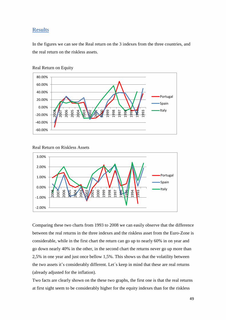
49

Results

In the figures we can see the Real return on the 3 indexes from the three countries, and

the real return on the riskless assets.

Real Return on Equity

Real Return on Riskless Assets

Comparing these two charts from 1993 to 2008 we can easily observe that the difference

between the real returns in the three indexes and the riskless asset from the Euro-Zone is

considerable, while in the first chart the return can go up to nearly 60% in on year and

go down nearly 40% in the other, in the second chart the returns never go up more than

2,5% in one year and just once bellow 1,5%. This shows us that the volatility between

the two assets it’s considerably different. Let´s keep in mind that these are real returns

(already adjusted for the inflation).

Two facts are clearly shown on the these two graphs, the first one is that the real returns

at first sight seem to be considerably higher for the equity indexes than for the riskless

-60.00%

-40.00%

-20.00%

0.00%

20.00%

40.00%

60.00%

80.00%

20

08

20

07

20

06

20

05

20

04

20

03

20

02

20

01

20

00

19

99

19

98

19

97

19

96

19

95

19

94

19

93

Portugal

Spain

Italy

-2.00%

-1.00%

0.00%

1.00%

2.00%

3.00%

20

08

20

07

20

06

20

05

20

04

20

03

20

02

20

01

20

00

19

99

19

98

19

97

19

96

19

95

19

94

19

93

Portugal

Spain

Italy

50

asset, and the second is that the volatility is also way bigger in the first case than in the

second.

In the following table we can see the means of real returns in the equity indexes and in

the riskless assets.

Real Return on

equities (mean)

Real Return on

riskless assets – Euro

Zone (mean)

Equity Premium

Portugal 5,86% 0,38% 5,48%

Spain 9,22% 0,47% 8,75%

Italy 5,45% 1,03% 4,42%

Average 6,84% 0,63% 6,21%

In the first sight this study goes in the encounter of the previous literature where the

average Equity Premium is very high (6,21%) even bigger than the previous literature

where it was about 6%.

The next question seems to be natural: Why does this fact happens?

The first reason seem to be obvious some may argue, If the stocks are riskier (have

more volatility than the bonds) investors demand a premium to bear such a risk. There

is no doubt that volatility is higher in stocks then in bonds, but is that fact enough to

affirm that stocks are really more risky than bonds?

The CAPM was already accessed and criticized in this paper; nevertheless it is still an

important financial instrument in nowadays. CAPM has a linear relationship between

the betas (systematic risk) and the expected return, therefore riskier stocks will tend to

have bigger returns when the market is bullish and lower returns when the market is

bearish because CAPM captures the good times and bad times depending on the market

total return.

Other perspective used in traditional finance is that investors like to have a smooth level

of consumption over time; insurance policies are classic examples of this situation,

where people tend to buy them even though most of them have low probability of

51

outcome. Following this logic and keeping in mind that stocks have bigger volatility

than bonds; investors prefer bonds to stocks because they can have a more “reliable”

and certain outcome, smoothing the earnings and therefore consumption over time.

“Unfortunately” this explanations do not seem to be convincing the all puzzle (even

though that they can explain a part of it) like it was said before only 1% can be

explained based on the standard theory to estimate adjusted-risk returns.

“We now have a bigger puzzle on our hands” (Constantinides et al 2002), in relation to

the fact that investors had ignored the equity premium in the last decades.

Behavioural Finance explanations

The two preferences based theories which were explained previously in this paper are

the cornerstones of Behavioural Finance in order to try to explain this puzzle.

Prospect theory

In 1995 Bernatzi and Thaler linked for the first time prospect theory with the equity

premium puzzle.

The aim of the study was to see how an investor with prospect theory type preferences

would construct his portfolio within stocks and T-Bills.

Like was discussed before Prospect theory states that people in general perceive wins

and losses differently, when choosing between different types of gambles they compute

the gains and losses for each one selecting the one with the highest prospect utility.

Talking more specifically about investors in the financial markets, taking this theory as

background investors will choose the composition of their portfolios (between stocks

and riskless investments) computing for each allocation the gains and losses in the value

of the positions that they have, this means that they will choose the position with the

highest prospect utility.

52

This can be shown by the following:

Rf,t +1 -» return on riskless security

Rt+1 -» return on the stock

W -» Fraction of wealth invested in the stock

v -» captures loss aversion

A very important aspect of this model is how to define the difference between t and t+1,

we know that investors are very different one from the other and they have different

goals and different time horizons. In one hand we can have an investor which wants to

make profits in a short term therefore making more transactions and trying to beat the

market (the so called speculator) and in the other hand we can have other investor which

has a long time perspective horizon.

Naturally the v – loss aversion will matter more for the speculator, which evaluates his

portfolio results in a shorter time period (because stocks will most likely have losses in

short time periods than in long periods) than the long term investor which will have a

way smaller probability of losing money.

With this fact into consideration this model calculates how often an investor needs to

evaluate his own portfolio in terms of losses and gains in order to be indifferent between

having positions in stocks or riskless securities.

The result was 1 year, the explanation for this time frame seems to be that people are

largely influenced by the information which they receive, and as the generality of

mutual funds show their reports in a year basis and the taxes are also paid and calculated

in the same time framework this result makes sense.

With this being said, if the investors get their utility from annual based evaluations and

they are loss averse, this loss aversion will therefore lead to a demand for a higher

equity premium from part of the investors. This model gives us some interesting

behavioural reasons for the high historical equity premium, but without a doubt has

some weak points, as it doesn’t access an inter temporal model with consumption

choice and therefore is unable to explain why even though stocks have a way higher

53

historical return than riskless securities investor seem reluctant to hold to them.

Bareberis, Huang and Santos (1991) start their paper with the same premise that

investors evaluate their portfolios once a year. They capture the utility taken from

consumption but also and more important the utility from the changes in the value of

their positions in the risky assets between t and t+1:

The first part of the equation shows the utility from consumption. And the second part

the utility from the changes in the positions.

The gains and losses for the utility are captured by:

The 2.25 is taken from Tversky and Kahneman´s (1992) study of attitudes towards

timeless gambles.

This form captures the loss aversion of the investors but fail to show the different

perceptions from investors regarding wins and losses.

This model shows that loss aversion can show the excess of premium, but it highly

depends on the second part of the equation which shows the utility that investors give to

changes in their positions in terms of gains and losses.

These assumptions can be explained in two different ways a non-consumption utility,

where investors perceiving a lost in their positions regret their past decisions. The other

one is consumption-related utility where investors used to some habit level of

consumption will not want to lose it, and despite the right thing to do is to merge all the

risks together and then compute the probability of consumption falling below the habit

level, most of the investors for one or other reason just consider the risk in the risky

assets, therefore only considering the wins and losses in the stock market.

54

The big criticism to these two models without a doubt will be the fact that they consider

that all investors evaluate their portfolios within the same time horizon of one year, and

in practice it is a bit hard to believe so.

In order to access this problematic Tversky, Kahneman and Schwartz (1997) made an

experimental test where they used three different groups of people, and told them to

allocate their wealth as they pleased, for that two investment funds results are showed,

these funds try to replicate at the maximum a stock variation

- Group A – The results are presented monthly

- Group B – The results are presented annually

- Group C – The results are presented in a five year level

In the end of all observations individuals are asked to allocate their wealth.

The results were clear, in average the individuals of group A allocate their wealth in less

proportion in stocks comparing to the other groups (let’s keep in mind that the funds

had the same results, but were presented in different time frames).

These results are in accordance with the idea that people evaluate the wins and losses in

how the information is presented. The individuals of group A, were presented with

monthly results, therefore with more frequent losses.

Ambiguity aversion

Previously on this paper was discussed how people tend not to like gambles where the

outcome is not known, in the financial markets this assumes a vital importance, as the

investors will most definitely not know the stock return with certainty.

With this in mind many papers were published on this matter, most of them take the

premise that the investor will react to ambiguity trying to guard against word case

misspecification, this means that investors will entertain a range of possibility

probability distributions and will act to maximize the minimum expected utility,

therefore the investor has a reference probability distribution in mind but wants to make

sure that his decisions are correct even if the reference model is not the most accurate

one.

55

In the financial markets, this can take an important role, if the model for stock returns is

not the most accurate one, investors will demand a bigger equity premium that will

work as a compensation for the perceived ambiguity in the probability distribution.

Bottom line is that stock returns are highly unpredictable, and with this is in mind

investors will not be that keen to hold stocks (mainly the most risky, and therefore most

unpredictable) this ambiguity aversion can explain some of the puzzle.

Unfortunately Maenhout (1999) show us that even though ambiguity aversion can solve

some part of the puzzle, it cannot solve it all because in order to explain the entire

equity premium would be necessary a very high and therefore very unlikely concern

about misspecification of the model on stock returns.

X - Size Premium Puzzle

Introduction

When Fama and French (1992) divided in deciles the stocks according the market

capitalization (number of outstanding shares times the unit price per share) in the

NYSE,AMEX and NASDAQ they realize that the smallest decile had an average return

0.74% per month higher than the largest one.

If we take in consideration the CAPM (which was discussed previously in this paper),

this fact is considered to be an anomaly which cannot be explained, because that even

though the betas (risk) of the smallest decile stocks are higher than the ones from the

largest one, the differences among the betas and therefore the risk difference can not

reflect all the difference in the average returns.

So once again the main model from the rational models and from the traditional finance

paradigm show flaws that cannot be ignored.

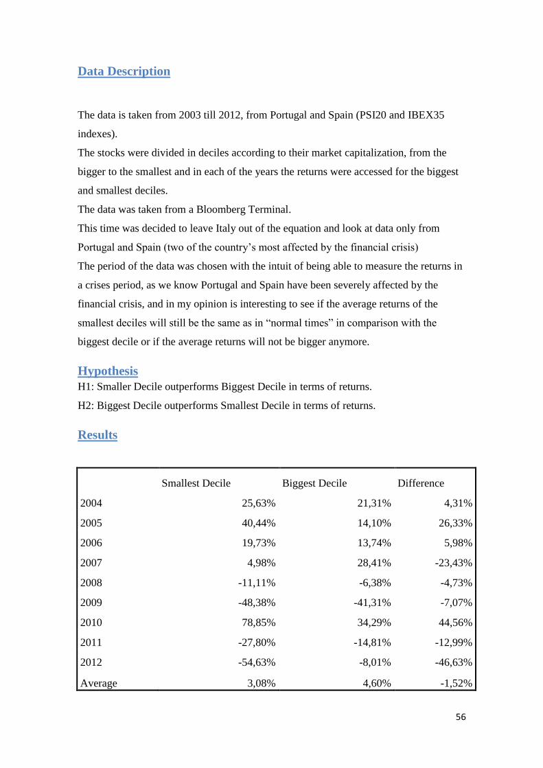
56

Data Description

The data is taken from 2003 till 2012, from Portugal and Spain (PSI20 and IBEX35

indexes).

The stocks were divided in deciles according to their market capitalization, from the

bigger to the smallest and in each of the years the returns were accessed for the biggest

and smallest deciles.

The data was taken from a Bloomberg Terminal.

This time was decided to leave Italy out of the equation and look at data only from

Portugal and Spain (two of the country’s most affected by the financial crisis)

The period of the data was chosen with the intuit of being able to measure the returns in

a crises period, as we know Portugal and Spain have been severely affected by the

financial crisis, and in my opinion is interesting to see if the average returns of the

smallest deciles will still be the same as in “normal times” in comparison with the

biggest decile or if the average returns will not be bigger anymore.

Hypothesis

H1: Smaller Decile outperforms Biggest Decile in terms of returns.

H2: Biggest Decile outperforms Smallest Decile in terms of returns.

Results

Smallest Decile Biggest Decile Difference

2004 25,63% 21,31% 4,31%

2005 40,44% 14,10% 26,33%

2006 19,73% 13,74% 5,98%

2007 4,98% 28,41% -23,43%

2008 -11,11% -6,38% -4,73%

2009 -48,38% -41,31% -7,07%

2010 78,85% 34,29% 44,56%

2011 -27,80% -14,81% -12,99%

2012 -54,63% -8,01% -46,63%

Average 3,08% 4,60% -1,52%

57

The results of my study do not go in accordance with the literature (Fama and French

1992) in which the smallest decile has an average superior return comparing to the big

one.

In my study the biggest decile from 2004 to 2012 outperforms the smallest in 1,52%,

which at the first sight goes really against the literature.

But once again, the aim in choosing this last decade was to see the behaviour of such

stocks in crisis periods.

If we take a “deeper look” in each of the years that are being accessed, we can a see an

interesting fact, in the years of 2004, 2005, 2006 and 2010 the smallest decile

outperforms the biggest one, specially in 2010 where the difference was of about 45%,

an impressive number without a doubt.

In the other hand in 2007, 2008, 2009, 2011 and 2012 the biggest decile outperform the

smallest, with special attention to 2012 where the difference is about 47%, once again a

huge difference.

Looking specifically to the recent economical story of Portugal and Spain (since 2004),

we can characterize the times of bull market, bear market and the so-called double-dip.

-80.00%

-60.00%

-40.00%

-20.00%

0.00%

20.00%

40.00%

60.00%

80.00%

100.00%

Smallest Decile

Biggest Decile

Difference

58

And it is very interesting to observe that in years of Bull Market the smallest decile

outperformed the biggest while in years of bear market the opposite happened.

Following the internet bubble burst of 2000, which had make severe losses in the stock

markets until sensibly 2003, countries like Portugal and Spain lived a bull market

characterized by high returns until 2008, when the global economic crisis stroked.

In 2010 the markets corrected from these losses, making the investors believe that a new

bull market was coming and the worst part of the crisis was already part of the past.

Unfortunately the southern European countries which had high debt levels entered in a

economic recession due to the downgrade of the republic grades by the rating agencies

and others macro-economic factors.

Countries like Portugal needed the help of the European Institutions in order to be able

to finance themselves. This triggered “the second part of the crisis” where the stock

markets in Portugal and Spain double-dip (after huge losses, and good recuperation,

again new huge losses).

In the following table and charts we can observe this evolution:

Date IBEX35 PSI20

2012 13895.8 5071.43

2011 17157.8 5494.27

2010 18598.8 7588.31

2009 21360.1 8463.85

2008 15447.7 6341.34

2007 24327.5 13019.4

2006 21974 11197.6

2005 16152.2 8618.67

2004 13241.2 7600.16

2003 10935 6747.41

2002 8272.4 5824.7

2001 11255.4 7831.49

2000 11981 10404.09

1999 15077.2 11960.51

1998 12556.3 10998.92

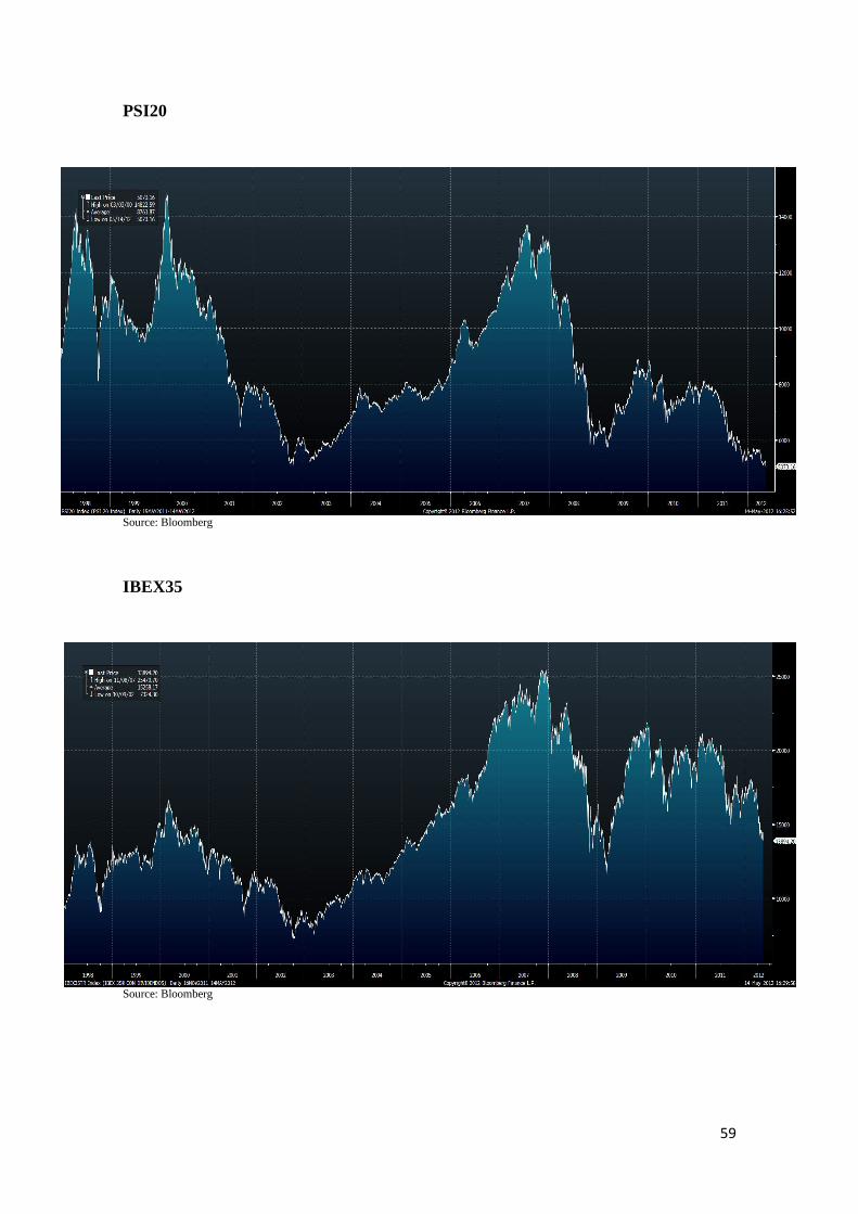
59

PSI20

Source: Bloomberg

IBEX35

Source: Bloomberg

60

With this being said, we can observe and conclude that the stocks from the biggest

deciles hold better in bearish periods and that the stocks from the smallest period

“explode” in bullish periods.

We know that the stocks from the smallest deciles have bigger betas, therefore have

bigger volatilities and bigger risk than the ones from the biggest one. Nevertheless the

difference in the average returns cannot again be explained taking in consideration only

this aspect.

According to Gompers and Metrick (2001), the size premium has been reduced

significantly during the last decade. This observation results from the fact that

institutional investors had grown in size and in number in the last decade, putting a

demand pressure on the stocks with a bigger market capitalization as these are the

stocks that they prefer.

Behavioural Finance Explanations

Despite the importance of Behavioural Finance in nowadays and the “help” that gave in

explaining several financial phenomena’s there are two phenomena’s (size premium and

dividends announcements) in which Behavioural Finance has some difficulties and has

not get into a consensus within the financial community.

Nevertheless, some models and biases from investors can be in great “help” to not

explain the phenomena in the whole plenitude, but giving some pointers and facts for

further discussion and study.

Taking as a premise the work of Gompers and Metrick (2001), that like it was said

before argue that institutional investors have preference for the stocks with the biggest

market capitalization.

In theory this investors assume the role of the “market sharks” they are the ones with

the better Know-How, access to the best information and overall they are the ones that

are not biased and “know what they are doing”.

In the other hand, even though those institutional investors had grown in the past, the

small, private, “normal” investor still has a major role in the market.

61

The market capitalization is calculated on the multiplication of the individual price of a

share with the number of shares outstanding in the market. So obviously the individual

price of a share assumes a great importance in the deciles calculation.

Why is important this differentiation between institutional investors and the small

investors?

If institutional usually prefer the stocks with the biggest stock details, it is not a secret

that the small investors which by far do not have the same wealth resources or know-

how of the institutional investors, prefer the small ones instead.

This comes from the fact that illusionary these stocks can be considered to be cheap or

undervalued, as they have small unitary prices, the so called penny stocks.

In reality there is no real connection between the fundamental value of the stock and the

fact of the stock as a big or a small price.

But without a doubt these stocks are more demanded by the small investors, it can be by

a simple thought of easy money as they see the small price of a unitary share, can be by

the illusion of having a bigger number of shares in their portfolios (as with small price

shares they can buy a bigger a amount with their limited dispensable wealth).

Small investors start therefore researching by themselves on these “cheap” stocks, with

their limited means, which take us to a very important bias, when investors gather the

information by themselves instead of using public information, they tend to be more

confident and have a special “feeling” for the stock itself.

Valuing their information very preciously they bet on the stocks creating a demand

pressure in the small market capitalization stocks, pushing therefore these stocks up.

The bottom line is that this differentiation is important because in general if the

institutional investors are the ones holding the stocks with the biggest market

capitalizations and the small investors holding the ones with the smallest capitalization,

this can help to this puzzle because in bull markets where small investors perceiving

stocks with small prices rapidly bet on them pushing the price up, and in bear markets

when the stocks start to decrease value, their pessimism is accentuated and rapidly sell

the stocks pushing their price even lower.

62

In the other hand institutional investors, which do not look at the unitary price of the

share but at his fundamentals (ratios, report analysis etc), trying to perceive in reality

which is the fundamental value of the share and act accordingly, will therefore not buy

or sell shares in the same premises as the biased small investors.

This can help to explain the reason why large stocks hold better in bearish markets, and

small stocks “explode”during bullish markets.

According to Barberis, Shleifer and Vishny (1998), the fact of the erratic formation of

future cash flows using public information contributes as well to this phenomena. As

investors are biased by numerous biases such as conservatism, tendency to underweight

new information, representativeness and the law of small number, where investors using

short samples characterize the market as a whole based on that sample.

Once again the behaviour and following biases of the investors assume a central role in

the explanation.

63

Conclusion

Within these ten chapters I tried to access the premises and cornerstones of both

paradigms, and explain in how behaviour finance takes off where the traditional finance

stops.

As I presented the both theories one thing starts to appear clear, the financial markets

need both of them, it is not possible continue with the old model of the traditional

finance by itself, but in the other hand Behaviour Finance like it was said starts from

where the traditional paradigm stops, so it cannot be used by itself.

If in one hand we need the traditional paradigm to show how the markets function in a

mechanic way, we also need the behavioural finance who can explain how the market

players behave in the most varied situations.

The living prove of this affirmation is in chapter VIII where using the both paradigms it

is possible to achieve a “perfect” portfolio for the investor, using one or the other on

itself will for sure not be optimal and in many cases highly risky in return terms.

As we get to the last chapters two of the puzzles which have generated a lot of

discussion in the last decades and are just anomalies for the traditional finance, can be

viewed in a different perspective that helps to explain these puzzles, “The Behavioural

Finance perspective”.

There is still a long way to go in the behavioural finance perspective, let’s not forget

that comparing to the traditional paradigm it is very recent, but one thing is undeniable

its importance has grown and has helped explaining and accessing problems that could

simply just not be explained before.

Also the two cornerstones of Behaviour Finance are very important and they have been

helping to change the view that the general financial community had on Efficient

Markets and Rationality.

64

Bibliography

Aloysius A. J. (2005), “Ambiguity aversion and the equity premium puzzle: A re-

examination of experimental data on repeated gambles”, The journal of Socio-Economics

34:635-655

Alpert, M. and Raiffa, H. (1982).” A progress report on the training of probability

assessors”. Cambridge University Press.

Barberis, N., Shleifer A. and Vishny R. (1998), “A model of investor sentiment”, Journal of

Financial Economics 49:307−345.

Benartzi S., and R. Thaler (1995), “Myopic loss aversion and the equity premium puzzle”,

Quarterly Journal of Economics 110:75−92.

Benartzi, S., and R. Thaler (2001), “Naive diversification strategies in defined contribution

savings plans”, American Economic Review 91:79−98.

Camerer F. C. (1998) “Prospect theory in the wild: Evidence from the field”, California

Institute of Technology Pasadena, Social Science working paper 1037

Constantinidies, G., Donaldson J., Mehra, R., (2002) “Junior Can't Borrow: A New

Perspective of the Equity Premium Puzzle”. Quarterly Journal of Economics, 2002, 117(1),

pp. 269-96.

Coval, J., and Moskowitz T. (1999), “Home bias at home: local equity preference in

domestic portfolios”, Journal of Finance 54:2045−2073.

Daniel, K., Hirshleifer D. and Subrahmanyam A. (1998), “Investor psychology and security

market under- and overreactions”, Journal of Finance 53:1839−1885.

Daniel, K., D. Hirshleifer and A. Subrahmanyam (2001), “Overconfidence, arbitrage and

equilibrium asset pricing”, Journal of Finance 56:921−965.

Heath C, Tversky A., (1991) “Preference and Belief: Ambiguity and Competence in Choice

under Uncertainty” Journal of risk and uncertainty, 4:5 - 28

Fabozzy J. F., Gupta F., and Markowitz M. H. (2002) “The Legacy of Modern Portfolio

Theory”, The journal of investing Fall 2002

Fama, E. (1965) “The Behavior of Stock-Market Prices” The Journal of Business, Vol. 38,

No. 1. (Jan., 1965), pp. 34-105.

Fama, E. (1970), “Efficient capital markets: a review of theory and empirical work”,

Journal of Finance 25:383−417.

Fama, E., and French K. (1992), “The cross-section of expected stock returns”, Journal of

Finance 47:427−465.

Fama, E. (1998), “Market efficiency, long-term returns and behavioral finance”, Journal of

Financial Economics 49:283−307.

65

Fox C, Tversky A., (1995) “Ambiguity Aversion and Comparative Ignorance”

The Quarterly Journal of Economics, Vol. 110, No. 3. pp. 585-603.

Friedman, M. and L. Savage (1952), “ The Expected Utility Hypothesis and

the Measurability of Utility ”, Journal of Political Economy , 60, 463-474.

Friedman, M. and L. Savage (1948), “The utility analysis of choices involving risk” The

Journal of Political Economy, Vol. 56, No. 4, pp. 279-304

Froot, K., and Dabora E. (1999), “How are stock prices affected by the location of trade?”,

Journal of Financial Economics 53:189−216.

Gompers P., Metrick A. (2001) “Institutional Investors and Equity Prices” Quarterly

Journal of Economics Vol 11 No1, pp 229-259.

Harris, L., and Gurel, E. (1986). “Price and volume effects associated with changes in the

S&P 500 list: New evidence for the existence of price pressures.” Journal of Finance

41:815–29.

Honghui C., Gregory N., and Vijay S. (2004) “The Price Response to S&P 500 Index

Additions and Deletions: Evidence of Asymmetry and a New Explanation” The Journal of

Finance • VOL. LIX, NO. 4

Kendall, Maurice (1953). “The Analysis of Economic Time Series”, Journal of the

Royal Statistical Society, Series A, 96, pp. 11-25.

King A. M., Leape I. J. (1998) “Wealth and portfolio composition: Theory and evidence”

Journal of Public Economics 69:155-193

Liu, Q.,&Song,F.(2001).”The rise and fall of Internet stocks: Should financial analysts be

blamed?” Working paper,University of HongKong

Lopes, L., Oden, G. (1999) “The Role of Aspiration Level in Risky Choice: A comparison

of cumulative prospect theory and SP/A Theory” Journal Of Mathematical Psychology,

Volume 43, Issue 2 pp 286-313.

Maenhout, P., (1999) “Robust portfolio rules and asset pricing” Working paper, Harvard

University

Markowitz H. (1952) “Portfolio Selection” The journal of Finance 1:77-91

Mehra, R., and E. Prescott (1985), “The equity premium: a puzzle”, Journal of Monetary

Economics 15:145−161.

Scheinkman A. J., and Wei X. (2003) “Overconfidence and Speculative Bubbles”, Journal

of Political Economy, 2003, vol 111, no. 6

Sharpe, W. (1964). “Capital asset prices: A theory of market equilibrium under conditions

of risk”, Journal of Finance, 19 (3), 425-442

66

Shleifer, A., Vishny, R. “The limits of arbitrage” The Journal of Finance, Vol. 52, No. 1.

(Mar., 1997), pp. 35-55

Shefrin, H., and Statman M. (1985), “The disposition to sell winners too early and ride

losers too long”, Journal of Finance 40:777−790.

Shefrin H., and Statman M. (2000), “Behavioral Portfolio Theory”, Journal of Finance and

Quantitative Analysis, Vol. 35, No.2

Ross S. (1976) “The arbitrage theory of capital asset pricing”, Department of economics

and Finance, University of Pennsylvania, Journal of Economy Theory 13, 341-360

Thaler H. R., and Benartzi S. (2004) “Save more tomorrow: Using behavioural Economics

to Increase Employee Saving” Journal of Political Economy vol 112 no.1 pt 2

Tversky, Amos and Kahneman, D. (1974) “Judgment under Uncertainty: Heuristics and

Biases” Science, New Series, Vol. 185, No. 4157 pp. 1124-1131.

Weber, M., and Camerer F. B. (1998) “The disposition effect in securities trading:

an experimental analysis” Journal of Economic Behaviour and Organization 33:167-184