ms excel 2010 - ncl.ac.uk · there are two ways to filter a list in microsoft excel i) using the...

MS Excel 2010

Analysing Data Using Formulae

& Pivot Tables

User Guide

NOMAS TRAINING & CONSULTANCY LTD

Dissington Hall, Ponteland, Northumberland

Tel : 01661 820 960 e-mail : [email protected] Web : www.nomas.co.uk

“ Because Training Matters ”

CONTENTS

INTRODUCTION .............................................................................. 1

Moving Around Your Spreadsheet .................................................................. 2

CONDITIONAL FORMATTING ........................................................... 4

Setting A Conditional Format ........................................................................ 4

Using Formulae As Conditions ....................................................................... 6

Style Sets ................................................................................................... 7

Identifying All Cells With Conditional Formatting.............................................. 8

Editing / Deleting Conditions ......................................................................... 9

SORTING AND FILTERING DATA ................................................... 10

Sorting A List By A Single Column ............................................................... 10

Sorting A List By Multiple Columns .............................................................. 10

Sorting A List By Colour ............................................................................. 12

Filter A List ............................................................................................... 14

Filter A List Using AutoFilter ........................................................................ 15

RE-ORGANISING DOWNLOADED DATA.......................................... 17

Converting Text To Columns – Parsing Data.................................................. 17

Removing Spaces ...................................................................................... 20

Removing Non-Printing Characters .............................................................. 20

CALCULATIONS USING FORMULAE ................................................ 21

Creating A Simple Formula ......................................................................... 22

Formulae Involving Cell References ............................................................. 22

Addition Of Columns Or Rows ..................................................................... 23

Copying Formulae – Relative & Absolute References ...................................... 23

Formulae Using Functions ........................................................................... 25

Using IF Statements .................................................................................. 26

Using VLOOKUP ......................................................................................... 27

Conditional Sums ...................................................................................... 30

Extracting Data from the Left or Right of a Cell ............................................. 32

Combining Cell Content .............................................................................. 33

PIVOT TABLE ................................................................................ 34

What Is A Pivot Table ? .............................................................................. 34

The Pivot Table Wizard ............................................................................... 35

Creating Pivot Filters .................................................................................. 38

Changing Date Grouping ............................................................................ 39

Adding Sub Totals ..................................................................................... 39

Re-Designing A Pivot Table ......................................................................... 41

Drilling Down Into The Data In A Pivot Table ................................................. 41

Slicers ...................................................................................................... 42

Create A Slicer In An Existing Pivot Table ..................................................... 42

Format A Slicer ......................................................................................... 43

Delete A Slicer .......................................................................................... 44

Updating A Pivot Table ............................................................................... 44

Creating A Chart From A Pivot Table ............................................................ 44

Re-Organising The Pivot Table .................................................................... 45

Adding Columns And Rows ......................................................................... 45

Removing Columns And Rows ..................................................................... 45

Changing The Summary Functions ............................................................... 46

Hiding / Displaying Sub & Grand Totals ........................................................ 47

APPENDIX 1 - FUNCTION KEYS ..................................................... 48

Function Keys ........................................................................................... 48

CTRL Combination Shortcut Keys ................................................................ 50

Other Useful Shortcut Keys ......................................................................... 53

Nomas Training & Consultancy Ltd

Excel 2010 – Analysing Data Using Formulae & Pivot Tables Page 1

INTRODUCTION

This guide covers the analysis of data using formulae, functions & pivot tables,

within Excel 2010. To obtain maximum benefit from attending this training

session, you should have attended an introductory course or be an existing user of

Excel.

At the end of this course, each delegate will have an understanding of several key

functions used in data analysis & will be able to create formulae, use functions,

sort & filter data & analyse data using pivot tables.

COPYRIGHT

© Nomas Training & Consultancy Ltd 2014

This manual should not be copied or reproduced in any way, nor its contents used

for any purpose, which has not been specifically granted by Nomas Training &

Consultancy Ltd.



Moving Around Your Spreadsheet

A spreadsheet is made up of a matrix of columns and rows, into which text, dates

and numbers can be entered. Excel contains ;

16,384 Columns.

1,048,576 Rows.

When working in your spreadsheet you can move around by use of both the

mouse and the keyboard. You can also move around the spreadsheet using the

scroll bars or by using the following keyboard strokes ;

Moving On A Sheet

Arrow Keys Move up/down/left/right as required.

Page Up/Page Down Moves one screen up or down.

Tab / Shift + Tab Moves one cell left or right.

F5 Moves to the cell number that you enter.

Ctrl + Home Moves to cell A1.

Ctrl + Left Arrow Moves to the cell furthest to the left hand of the spreadsheet that contains data.

Ctrl + Right Arrow Moves to the cell furthest to the right hand of the spreadsheet that contains data.

Ctrl + Up Arrow Moves to the cell furthest to the top of the

spreadsheet that contains data.

Ctrl + Down Arrow Moves to the cell furthest to the bottom of the spreadsheet that contains data.

Selecting Cells

Shift + Left / Right

Arrow Keys Selects cells ‘one at a time’ to the left / right.

Shift + Up / Down Arrow Keys

Selects cells ‘one at a time’ up / down.

Ctrl + Shift + Left / Right Arrow Keys

Selects cells to the end of a ‘block of data’ in a row.

Ctrl + Shift + Up /

Down Arrow Keys

Selects cells to the end of a ‘block of data’ in a

column.



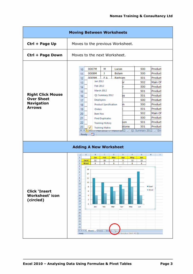
Moving Between Worksheets

Ctrl + Page Up Moves to the previous Worksheet.

Ctrl + Page Down Moves to the next Worksheet.

Right Click Mouse

Over Sheet Navigation Arrows

Adding A New Worksheet

Click ‘Insert Worksheet’ icon

(circled)



CONDITIONAL FORMATTING Excel can be used to highlight data that meets conditions that you specify. To

highlight formula results or other cell values that you want to monitor, you can

identify the cells by applying ‘Conditional Formats’.

Setting A Conditional Format

For instance, in an Orders data set, Excel can apply red shading to the cell, if the

‘Total Price’ is greater than £1,000 or blue shading if the ‘Total Price’ is less than

£1,000. To apply conditional formats to cells ;

1 Select the cells you want to format. In this example, select the ‘Total

Order’ cells only.

2 Select ‘Conditional Formatting’ from the ‘Home’ tab.

3 Select ‘Highlight Cell Rules’.

4 Then select an appropriate option e.g. ‘Greater than…



5 Enter the amount in the first dialogue box & then select the drop down

option in the second dialogue box, to set the appropriate formatting

options. Use ‘Custom Format’ if you want to set your own formatting

options.

6 Select the font style, font colour, underlining, borders, shading, or

patterns you want to apply.

7 To add another condition, repeat the steps above.

8 To review the conditional formats applied to the cells, use ‘Conditional

Formatting….Manage Rules’ from the ‘Home’ tab.

9 Here you can create new rules or modify / delete existing rules.



Using Formulae As Conditions

In the previous example, the cell colour in a single column (Total Order) was

changed. In order to apply the cell colour all the way across a row, then a formula

could be used.

1 Select the cells you want to format (the whole data set).

2 Select ‘Conditional Formatting….New Rule’ from the ‘Home’ tab.

3 Select ‘Use a formula to determine which cells to format’.

4 Enter a suitable formula & format for the cells & click ‘OK’.

5 In this example, the formula would be =$I2 > 1000.



Style Sets

Data Bars, Colour Scales & Icon Sets can also be used to format cells. In the

example below, ‘Total Prices’ can be marked with ‘Traffic Lights’ to indicate

whether the Total is less than £250, between £250 - £1,000 or over £1,000.



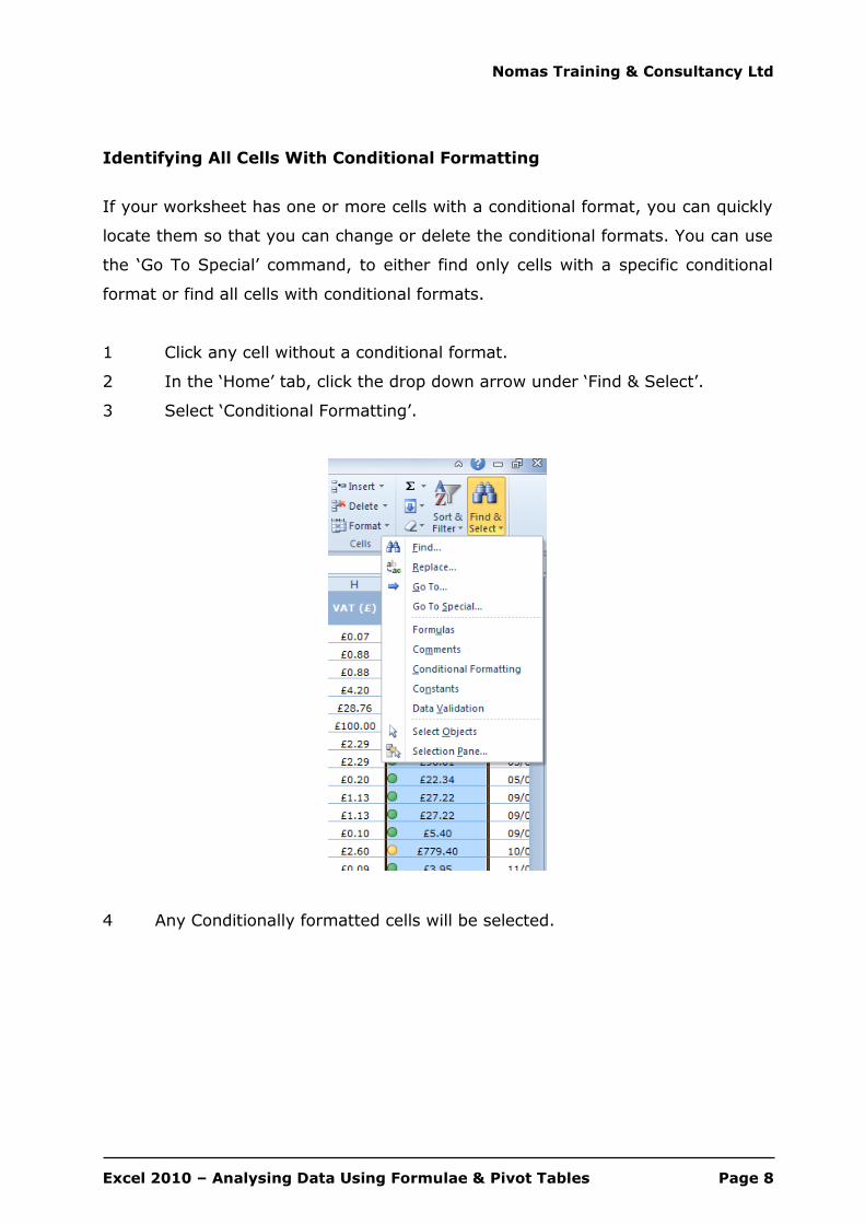
Identifying All Cells With Conditional Formatting

If your worksheet has one or more cells with a conditional format, you can quickly

locate them so that you can change or delete the conditional formats. You can use

the ‘Go To Special’ command, to either find only cells with a specific conditional

format or find all cells with conditional formats.

1 Click any cell without a conditional format.

2 In the ‘Home’ tab, click the drop down arrow under ‘Find & Select’.

3 Select ‘Conditional Formatting’.

4 Any Conditionally formatted cells will be selected.



Editing / Deleting Conditions

To delete a condition ;

1 Select your ‘Conditionally Formatted’ cells.

2 Select ‘Conditional Formatting….Manage Rules’ from the ‘Home’ tab.

3 Select the format to delete & click ‘Delete Rule’.

4 Edit a Conditional Format, in the same manner, by clicking ‘Edit Rule’.



SORTING AND FILTERING DATA Sorting A List By A Single Column

To sort data in ascending / descending order based on values in a single column ;

1 Click a cell in the column you want to ‘sort’.

DO NOT HIGHLIGHT MULTIPLE CELLS

2 Click the ‘Sort Ascending’ or ‘Sort Descending’ icon on the ‘Data’ tab.

Sorting A List By Multiple Columns

If you require a more complicated sorting procedure i.e. you want to sort by more

than one column, you will need the ‘Sort’ icon on the ‘Data’ tab. When you sort by

more than one column, the rows with duplicate items in the first column are

sorted according to the second column you specify. To do this ;

1 Click a cell in the column you want to ‘sort’.

2 Click the ‘Sort’ icon on the ‘Data’ tab.

3 Select the 1st sort options you want e.g. above, list is sorted by ‘Dept’.

4 Click ‘Add Level’.



5 Repeat the selection process, for the 2nd level.

The list above will be sorted by ‘Dept’ first, then within each department, by ‘Full

Name’.

6 Potentially, extra levels may be required, until you obtain the ‘Sort’ order

you require.



Sorting A List By Colour

If you have manually or conditionally formatted a range of cells, by cell colour or

font colour, you can also sort by these colours. You can also sort by an icon set

created through a conditional format.

In the above example, a Conditional Format has been applied to highlight

‘Delivery Bands’ ;

1 - 10 Days Green

11 - 20 Days Amber

Over 20 Days Red

Using the ‘Sort’ option, you can sort by colour ;

1 Click a cell in the data you want to ‘sort’.

2 Click the ‘Sort’ icon on the ‘Data’ tab.



3 Select the 1st sort option, e.g. ‘Delivery Band’, then in the ‘Sort On’

column, select the ‘Cell Colour’ option.

4 In the ‘Order’ column, select the colour & whether it is to be sorted ‘On

Top’ or ‘On Bottom’.

5 Then click ‘Add Level’ & repeat the process.

6 Make sure that you select the same column in the ‘Then by’ box and that

you make the same ‘On Top’ selection for your next colour.

7 Keep repeating for each additional cell colour, that you want included in

the sort.



The above settings, will sort the list with ‘Green’ at the top of the list, followed by

‘Amber’ then ‘Red’.

Filter A List

By filtering a list, you can display just the rows that meet the criteria you specify.

For example, in a list of names and addresses, you can see only the names of

people who live in Newcastle. There are two ways to filter a list in Microsoft Excel

i) using the ‘AutoFilter’ command or ii) the ‘Advanced Filter’ command, both on

the ‘Data’ tab.

The ‘AutoFilter’ command displays arrows next to the column labels in a list, so

you can select the item you want to display. Use the ‘AutoFilter’ command to

quickly filter rows using criteria in a single column.

The ‘Advanced Filter’ command, filters your list, as ‘AutoFilter’ does, but it does

not display arrows in column labels for criteria selection. Instead, you type criteria

in a criteria range on your worksheet.



Filter A List Using AutoFilter

For this procedure to work, your list must have ‘column labels’.

1 Select a cell in the list you want to filter.

2 Select ‘Filter’ from the ‘Data’ tab.

3 Click the arrow in the column, that contains the data you want to filter.

4 Remove the check mark from ‘Select All’.

5 Select the check box for the entry you want to filter & then click ‘OK’.

6 You can select multiple check boxes to filter on two or more items.

7 Alternatively, type your criteria in the ‘Search’ box.

8 You can create ‘Custom’ filters by using ‘Text Filters….Custom Filter’.



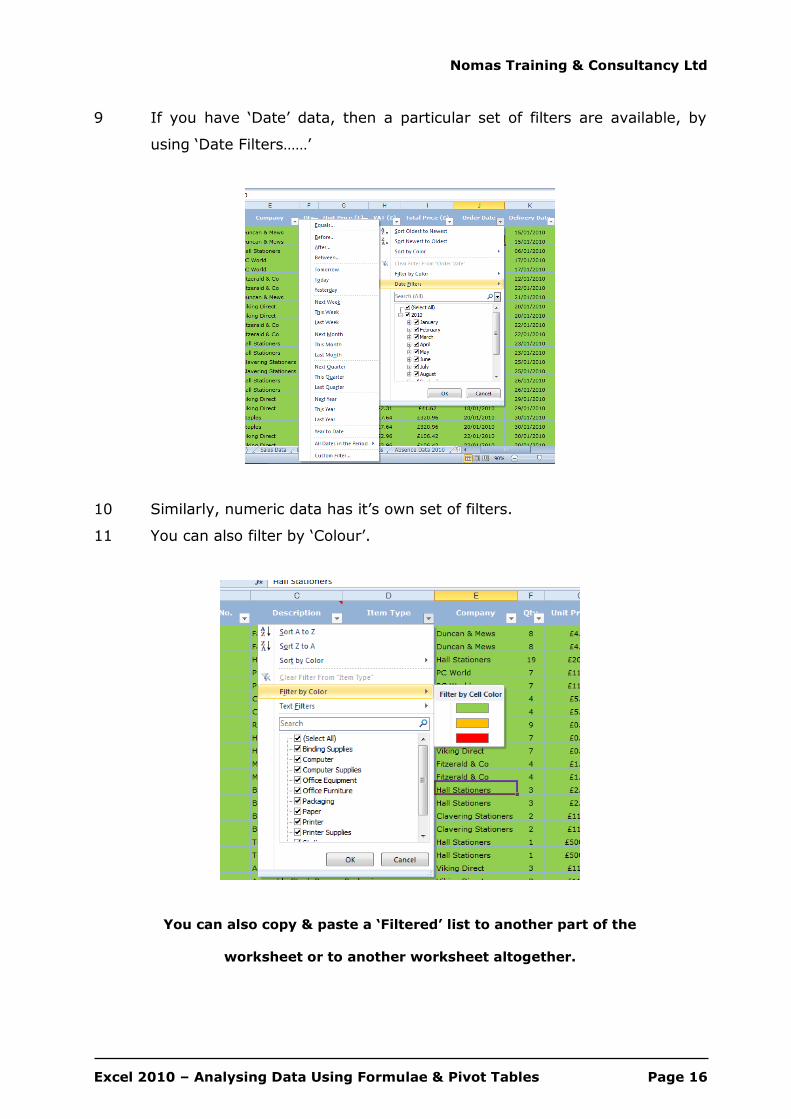
9 If you have ‘Date’ data, then a particular set of filters are available, by

using ‘Date Filters……’

10 Similarly, numeric data has it’s own set of filters.

11 You can also filter by ‘Colour’.

You can also copy & paste a ‘Filtered’ list to another part of the

worksheet or to another worksheet altogether.



RE-ORGANISING DOWNLOADED DATA

When data is downloaded (exported) from other database applications, there can

be several problems with the data ;

Data is contained within one column.

Data contains unwanted spaces (normally at the front of the data).

Data contains non-printing characters.

The spreadsheet below, demonstrates all of these problems.

Converting Text To Columns – Parsing Data

The data above is separated by a ‘,’ character & contains 5 parts of the address in

the same column. This data therefore needs to be spilt up (parsed) into 5 separate

columns.

1 Ensure you have sufficient (new) blank columns, to the right of the column

containing data. In the above example, 4 new columns are required.



2 Select all of the data in the column & then in the ‘Data’ tab, select ‘Text To

Columns’.

3 If the data has ‘separators’ e.g. ‘ , ’, select ‘Delimited’, then click ‘Next’.

4 Either select the ‘Delimiter’, or type it in the ‘Other’ box.

5 Click ‘Next’



6 Each column can be formatted before splitting the data.

7 Click ‘Finish’.

8 Assuming you have entered the required number of empty columns (as

described previously), click ‘OK’.

9 If you have not entered new columns, you will have to click ‘Cancel’ at this

point, insert the blank columns & then go through the procedure again.

10 The data will then be separated into the required number of columns & in

this example, the address will be split into the appropriate parts.



Removing Spaces

Use the TRIM function to remove all spaces from text, except for single spaces

between words.

=TRIM(S2)

The formula would need to be entered in a new column & then copied & pasted

(use ‘Paste Special’) to paste the ‘Values’ over the existing data.

Removing Non-Printing Characters

Occasionally, data which has been exported from another application, may contain

non-printing characters.

Use the CLEAN function to remove these characters from text.

=CLEAN(S2)

These 2 functions could be combined, in to a single formula.

=TRIM(CLEAN(S2))

In order that both operations are performed in a single formula, without the need

to enter 2 separate formulae.



CALCULATIONS USING FORMULAE Excel can perform calculations on your data. This can be done by using ‘formulae’

within your spreadsheet. All formulae within Excel have the equals sign (=) as the

first character.

All formulae within Excel have the equals sign (=) as the first character.

All standard arithmetic operators can be used ;

Operation Excel Key Example

Addition + (plus sign) =A1+B3

Subtraction - (minus sign) =A1-B3

Multiplication * (star or asterisk) =A1*B3

Division / (forward slash) = A1/B3

Exponential ^ (caret) =A1^2 (equiv to A1 squared)

Brackets ( ) (open / close brackets) =(A1+B3)/C4

The order that a calculation is performed is important to remember. Excel follows

the standard mathematical rules i.e. the following order is adopted ;

1 Anything in brackets is done first,….. then B

2 Orders e.g. squared, square root etc. O

3 Division. D

4 Multiplication. M

5 Addition. A

6 Subtraction. S

Thus, the following formulae ;

= 5+7*3 Produces the answer 26.

= (5+7)*3 Produces the answer 36.



Creating A Simple Formula

To create your own formula ;

1 Start with an equals sign =.

2 Enter the formula e.g. =54 / 7.

3 Press the ‘green tick’ on the toolbar or press the ‘ENTER’ key.

4 The cell will display the result of the formula.

5 The actual formula itself, will be visible in the ‘Formula Bar’.

Formulae Involving Cell References

Excel has the ability to perform calculations based on the content of other cells in a

spreadsheet (as in the example below).

1 Make the active cell, the cell where you want to put your formula.

2 Start with an equals sign =.

3 As you are using cell references, click in the first cell you require in your

formula (D2, in the example below).

4 Enter the required arithmetic operator e.g. *

5 Complete the remaining formula

6 Press the ‘green tick’ on the toolbar or press the ‘ENTER’ key.

7 The cell will display the result of the formula.

8 The actual formula itself, will be visible in the ‘Formula Bar’.



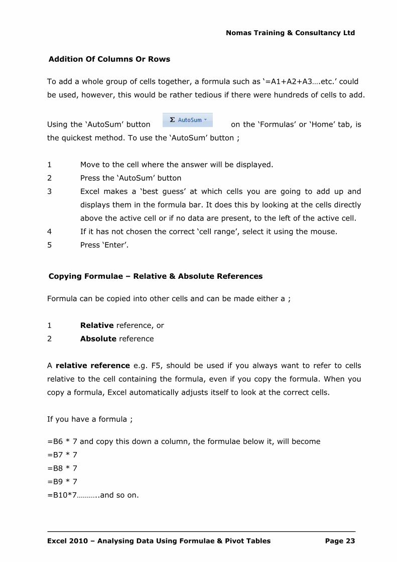
Addition Of Columns Or Rows

To add a whole group of cells together, a formula such as ‘=A1+A2+A3….etc.’ could

be used, however, this would be rather tedious if there were hundreds of cells to add.

Using the ‘AutoSum’ button on the ‘Formulas’ or ‘Home’ tab, is

the quickest method. To use the ‘AutoSum’ button ;

1 Move to the cell where the answer will be displayed.

2 Press the ‘AutoSum’ button

3 Excel makes a ‘best guess’ at which cells you are going to add up and

displays them in the formula bar. It does this by looking at the cells directly

above the active cell or if no data are present, to the left of the active cell.

4 If it has not chosen the correct ‘cell range’, select it using the mouse.

5 Press ‘Enter’.

Copying Formulae – Relative & Absolute References

Formula can be copied into other cells and can be made either a ;

1 Relative reference, or

2 Absolute reference

A relative reference e.g. F5, should be used if you always want to refer to cells

relative to the cell containing the formula, even if you copy the formula. When you

copy a formula, Excel automatically adjusts itself to look at the correct cells.

If you have a formula ;

=B6 * 7 and copy this down a column, the formulae below it, will become

=B7 * 7

=B8 * 7

=B9 * 7

=B10*7………..and so on.



If however, you want to refer to the same cell regardless of where the formula is on

the worksheet, use an absolute reference.

A ‘$’ sign should be placed before the column letter or row number (whichever is

appropriate), in order to ‘freeze’ the cell reference when it is copied.

If, in the above example, in Column G, cell F2 is multiplied by the contents of L1

and you want all the subsequent cells, to be multiplied by L1, then you should use

the formula =F2*L$1. In this example, L1 has become an absolute reference and

when you copy this formula, it will always retain L1, although changing the cell

numbers of column F.

=F2 * L$1

=F3 * L$1

=F4 * L$1

=F5 * L$1

=F6 * L$1…………and so on.



Formulae Using Functions

In addition to simple mathematical operators e.g. multiplication, subtraction etc.,

Excel has a variety of ‘Functions’, these are available via the ‘Insert Function’ icon,

on the ‘Formulas’ tab or the fx button, to the left of the ‘Formula Bar’.

The use of several of the most commonly used functions e.g. SUM, AVERAGE,

COUNT, were discussed in the ‘Introduction’ course.

Due to the large number of functions available, it is beyond the scope of this guide

to cover all of these functions, however, the following examples show how to use

some of the more commonly used functions. You can search for a function by

typing the function name, in the ‘Search for a function’ box & clicking the ‘GO’

button.



Using IF Statements

You can use the IF statement to determine if a particular ‘criteria’ is true or not,

and then produce a response depending on the outcome. For example, if you had

a ‘Production’ worksheet, detailing daily production figures & targets, you could

use an IF function, to check whether production targets, have been achieved.

The example above, uses an IF function (column ‘E’) to check production figures.

If you do not want both the ‘True’ & ‘False’ text to appear, you must use a blank

set of speech marks “” in the box, otherwise FALSE will be displayed in the cell.



Looking Up Values In A Table

You can look up the contents of various cells within a data set. For example, if an

item has a particular code, you simply enter the code number and the name of the

item, will be displayed.

Using VLOOKUP

This function looks down a vertical column of data until an appropriate value is

found. In the example below, an orders sheet is set up, so that when the ‘Item

No. is present in column ‘B’, it ‘looks up’ the ‘Description’, ‘Item Type’ &

‘Company’ & enters these into columns ‘C’, ‘D’ & ‘E’ respectively.

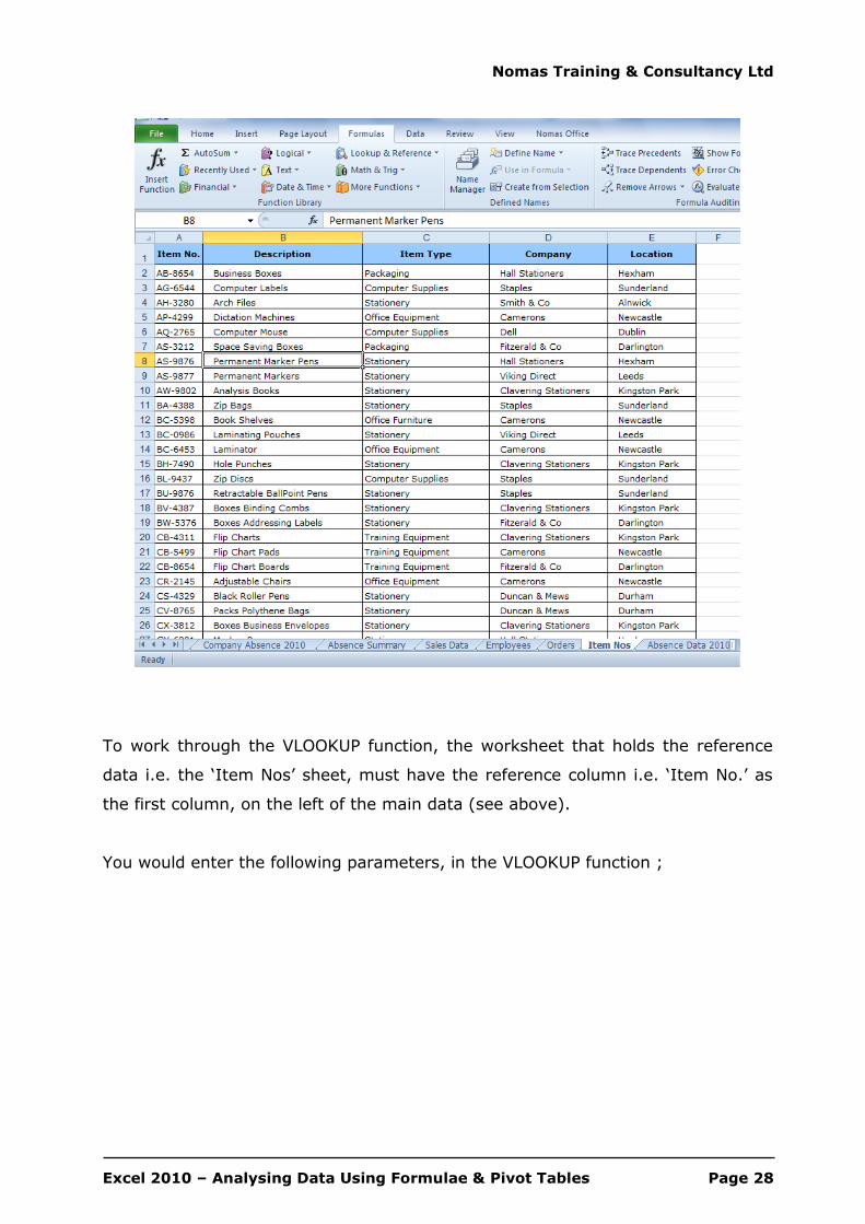
The ‘Description’, ‘Item Type’ & ‘Company’ are stored on a separate sheet ‘Item

Nos’ (above).



To work through the VLOOKUP function, the worksheet that holds the reference

data i.e. the ‘Item Nos’ sheet, must have the reference column i.e. ‘Item No.’ as

the first column, on the left of the main data (see above).

You would enter the following parameters, in the VLOOKUP function ;



You will thus end up with the following formula, in your cell.

=VLOOKUP(B2, 'Item Nos'!A:E,2,FALSE)

Where :

Lookup_value = Cell where Item No. is entered (B2)

Table_array = Area where Item No & Description are stored (Item Nos'!A:E)

Col_index_num = Second column, along to the right of column ‘A’ (2)

Range_lookup = Ensures an exact match is found (False)



Conditional Sums

To ‘Sum’ values in a list (that meet specific conditions) use the ‘SUMIF’ function.

The formula below, calculates the total cost of all courses, attended by Finance

employees.

=SUMIF(D:D,N2,L:L)

Where ;

Range Is the range of cells you want evaluated (D:D)

Criteria Is the criteria, in the form of a cell reference that defines which

cells will be added. E.g. in the above example, the Total Cost is

calculated, using a cell reference of ‘N2’, for the criteria.

Sum_range Are the actual cells to sum. The cells in ‘sum_range’ are summed

only if their corresponding cells in ‘range’, match the criteria (L:L).



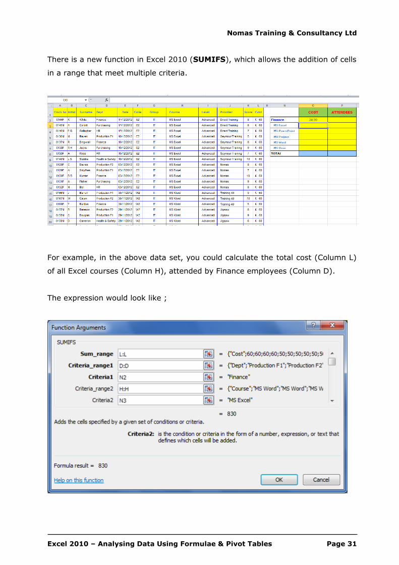
There is a new function in Excel 2010 (SUMIFS), which allows the addition of cells

in a range that meet multiple criteria.

For example, in the above data set, you could calculate the total cost (Column L)

of all Excel courses (Column H), attended by Finance employees (Column D).

The expression would look like ;



Extracting Data from the Left or Right of a Cell

If data in a cell, needs to be ‘split up’ or certain characters extracted from either

end of a data set, then the ‘Left’ or ‘Right’ function can be used. For example, if an

employees number was in the format 0045M, where the last character denoted

the gender of the person and the data was stored in Column A, then the final

character could be extracted using the formula ;

=RIGHT(A2,1)

Where ;

Text = cell containing data e.g. Clock No. (A2)

Num_chars = no. of charatcers from the right of this cell, to extract (1)



Combining Cell Content

It is possible to combine or join together information, from different columns on a

spreadsheet, using the ‘Concatenate’ function. E.g. if the employees ‘Surname’ &

‘Initial’, are stored in separate columns in a worksheet.

=CONCATENATE(E2," , ",D2)

Where ;

Text 1, 2, 3 etc = Cells to be combined (E2, D2)

“ ” = Use “ ” to indicate space between cells.



PIVOT TABLE What Is A Pivot Table ?

A Pivot Table is an interactive worksheet table that summarises and analyses data

from an existing list. You decide which of the fields (in the list) are to be arranged

in rows and columns. You can re-arrange the table very easily, in effect ‘twisting’

the data around - hence the name Pivot Table.

Most Excel spreadsheets are generally of the same format i.e. they contain a

series of fields (column headings) containing data in rows.

The following example shows a spreadsheet that contains information on the

training carried out within a company, from 2007-2013. It lists the delegate

details, training provider, course and cost of training. It contains a lot of

information & it is very difficult to get an overall ‘summarised’ view. This is where

the ‘power’ of a Pivot Table lies. They effectively display the result of a ‘database

analysis’.



The Pivot Table Wizard

You create Pivot Tables by using the Pivot Table Wizard. Although this only takes a

few moments, it is worth spending some time to decide how you want to

summarise your data. To create a Pivot Table ;

1 Select a cell in your data & select ‘Pivot Table’ from the ‘Insert’ tab.

2 The range of your data should be entered automatically, modify, if not

correct.

3 Select whether the pivot table is to be placed on a new worksheet or

within your existing worksheet.

4 Click ‘OK’.



5 You need to drag (or tick) the ‘Fields’ from the right hand side, onto the

appropriate lower part of the table (areas marked ‘Drag Fields Between

Areas Below’) & into the ‘Row’, ‘Column’, ‘Values’ areas.

VALUES This field contains the data that you want to summarise (often a numeric field).

ROW This is the field that you want to appear as rows

with labels down the side of the table.

COLUMN This is the field that you want to appear as columns

with labels across the top of the table.

REPORT FILTER See later.



6 The Pivot Table is created (next page).

7 You can have several field headings, in any one of these areas. Example

below has ‘Dept’, ‘Group’ & ‘Course’, in the ‘Row’ area.



Creating Pivot Filters

As it is not possible to read text in three-dimensions, all the fields that you want

to see in a pivot Table are ‘squashed’ into the row or column positions.

However, it is possible to create a third dimension to provide added flexibility to

your data. This is done by creating a Pivot Filter.

To create a Pivot Filter ;

1 Start the Pivot Table Wizard.

2 Complete steps as described previously.

3 In Step 5, move the field that you want to filter to the ‘Report Filter’ area.

4 Continue as described previously.

5 In the above example the ‘Course’ field has been added to the ‘Filter field,

so that the training can be filtered by ‘Course’.



Changing Date Grouping

If a ‘Date’ field is used in a Pivot Table, it does not automatically ‘group’ data by

month or year. Therefore, you need to set the grouping level, by right clicking on

the ‘Date’ area & selecting ‘Group’.

You can then set the level required, e.g. ‘Months’, ‘Quarters’ etc.

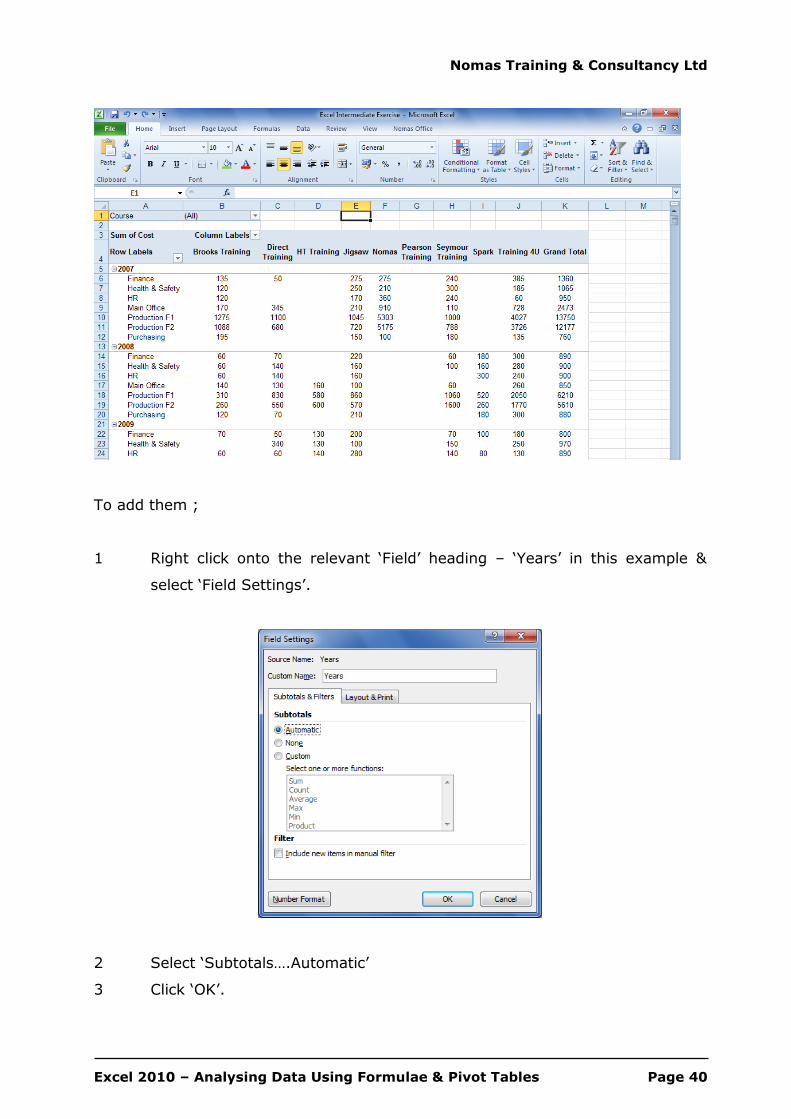
Adding Sub Totals

If ‘Sub-Totals’ are not automatically displayed, it is possible to add them

manually, in the example (over) the ‘Annual’ sub-totals do not appear

automatically.



To add them ;

1 Right click onto the relevant ‘Field’ heading – ‘Years’ in this example &

select ‘Field Settings’.

2 Select ‘Subtotals….Automatic’

3 Click ‘OK’.



Re-Designing A Pivot Table

There are 2 Custom Tabs, that are available when using a Pivot Table.

Pivot Table Tools – Options

Pivot Table Tools – Design

Commonly, this tab is used for selecting a particular colour scheme, ‘PivotTable

Style’, for your pivot table.

Drilling Down Into The Data In A Pivot Table

To see the ‘underlying’ data, in the Pivot Table, simply double click in the Pivot

Table data. For example, to see the ‘Employees Trained’ in HR, by the ‘Nomas’

training provider, double click in the appropriate cell e.g. 480 (below) & the data

will be copied into a new sheet.



Slicers

Slicers are easy-to-use filtering components, that contain a set of buttons that

enable you to quickly filter the data in a PivotTable, without the need to open

drop-down lists to find the items that you want to filter.

When you use a regular PivotTable filter to filter on multiple items, the filter

indicates only that multiple items are filtered, and you have to open a drop-down

list to find the filtering details. However, a slicer clearly labels the filter that is

applied and provides details so that you can easily understand the data that is

displayed in the filtered PivotTable report.

Create A Slicer In An Existing Pivot Table

1 Click anywhere in the PivotTable, for which you want to create a slicer.

2 On the ‘Options’ tab, click ‘Insert Slicer’.



3 In the ‘Insert Slicers’ dialog box, select the check box of the PivotTable

fields for which you want to create a slicer.

4 Click ‘OK’.

5 A ‘slicer’ is displayed for every field that you selected.

6 In each slicer, click the items on which you want to filter.

7 To select more than one item, hold down CTRL, and then click the items on

which you want to filter.

8 Click an item in the ‘Slicer’, to see the Pivot Table data.

Format A Slicer

1 Click the slicer that you want to format.

2 This displays the ‘Slicer Tools’, adding an ‘Options’ tab.

3 On the ‘Options’ tab, click the style that you want.



Delete A Slicer

Do one of the following ;

1 Click the slicer, and then press ‘DELETE’.

2 Right-click the slicer, and then click ‘Remove <Name of slicer>’.

Updating A Pivot Table

The Pivot Table does not change when you update your data in the source list. You

can update your Pivot Table, by ;

1 Selecting any cell within the Pivot Table.

2 Click the ‘Refresh’ icon, in the ‘Pivot Table Tools’ tab.

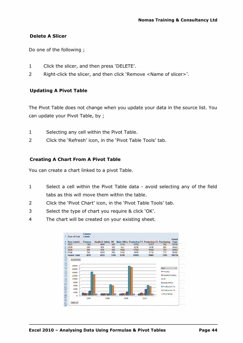
Creating A Chart From A Pivot Table

You can create a chart linked to a pivot Table.

1 Select a cell within the Pivot Table data - avoid selecting any of the field

tabs as this will move them within the table.

2 Click the ‘Pivot Chart’ icon, in the ‘Pivot Table Tools’ tab.

3 Select the type of chart you require & click ‘OK’.

4 The chart will be created on your existing sheet.



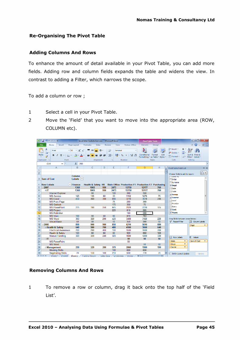
Re-Organising The Pivot Table

Adding Columns And Rows

To enhance the amount of detail available in your Pivot Table, you can add more

fields. Adding row and column fields expands the table and widens the view. In

contrast to adding a Filter, which narrows the scope.

To add a column or row ;

1 Select a cell in your Pivot Table.

2 Move the ‘Field’ that you want to move into the appropriate area (ROW,

COLUMN etc).

Removing Columns And Rows

1 To remove a row or column, drag it back onto the top half of the ‘Field

List’.



Changing The Summary Functions

Excel summarises data by summing numeric values (if the data fields contain text,

the Pivot Table displays counts of the values). You can change the summary

function or calculation type ;

1 Select a heading in the ‘Values’ area of the ‘Field List’.

2 Click the drop down arrow & select ‘Value Field Settings’.

3 In the ‘Summarise by’ list, select the desired summary function.



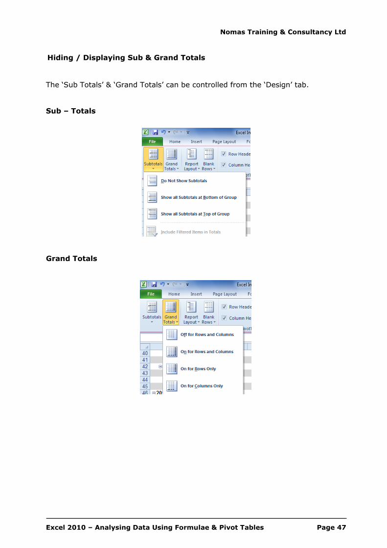
Hiding / Displaying Sub & Grand Totals

The ‘Sub Totals’ & ‘Grand Totals’ can be controlled from the ‘Design’ tab.

Sub – Totals

Grand Totals



APPENDIX 1 - FUNCTION KEYS

The following lists contain function key, CTRL combination shortcut keys and some

other common shortcut keys, along with descriptions of their functionality.

Function Keys

Key Description

F1

Displays the Microsoft Office Excel Help task pane.

CTRL+F1 displays or hides the ribbon.

ALT+F1 creates a chart of the data in the current range.

ALT+SHIFT+F1 inserts a new worksheet.

F2

Edits the active cell and positions the insertion point at the end of the cell

contents. It also moves the insertion point into the Formula Bar when editing

in a cell is turned off.

SHIFT+F2 adds or edits a cell comment.

CTRL+F2 displays the Print Preview window.

F3 Displays the Paste Name dialog box.

SHIFT+F3 displays the Insert Function dialog box.

F4 Repeats the last command or action, if possible.

CTRL+F4 closes the selected workbook window.

F5 Displays the Go To dialog box.

CTRL+F5 restores the window size of the selected workbook window.

F6

Switches between the worksheet, ribbon, task pane, and Zoom controls. In a

worksheet that has been split (View menu, Manage This Window, Freeze

Panes, Split Window command), F6 includes the split panes when switching

between panes and the ribbon area.

SHIFT+F6 switches between the worksheet, Zoom controls, task pane, and

ribbon.

CTRL+F6 switches to the next workbook window when more than one

workbook window is open.



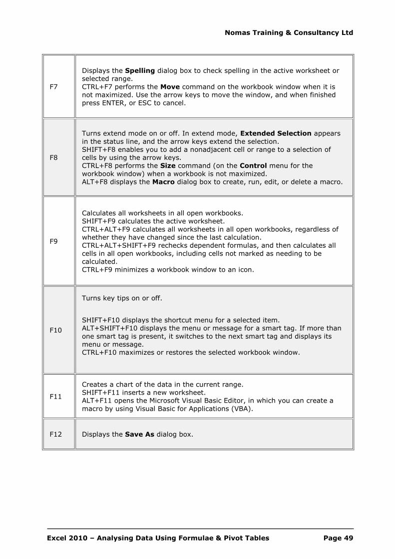
F7

Displays the Spelling dialog box to check spelling in the active worksheet or

selected range.

CTRL+F7 performs the Move command on the workbook window when it is

not maximized. Use the arrow keys to move the window, and when finished

press ENTER, or ESC to cancel.

F8

Turns extend mode on or off. In extend mode, Extended Selection appears

in the status line, and the arrow keys extend the selection.

SHIFT+F8 enables you to add a nonadjacent cell or range to a selection of

cells by using the arrow keys.

CTRL+F8 performs the Size command (on the Control menu for the

workbook window) when a workbook is not maximized.

ALT+F8 displays the Macro dialog box to create, run, edit, or delete a macro.

F9

Calculates all worksheets in all open workbooks.

SHIFT+F9 calculates the active worksheet.

CTRL+ALT+F9 calculates all worksheets in all open workbooks, regardless of

whether they have changed since the last calculation.

CTRL+ALT+SHIFT+F9 rechecks dependent formulas, and then calculates all

cells in all open workbooks, including cells not marked as needing to be

calculated.

CTRL+F9 minimizes a workbook window to an icon.

F10

Turns key tips on or off.

SHIFT+F10 displays the shortcut menu for a selected item.

ALT+SHIFT+F10 displays the menu or message for a smart tag. If more than

one smart tag is present, it switches to the next smart tag and displays its

menu or message.

CTRL+F10 maximizes or restores the selected workbook window.

F11

Creates a chart of the data in the current range.

SHIFT+F11 inserts a new worksheet.

ALT+F11 opens the Microsoft Visual Basic Editor, in which you can create a

macro by using Visual Basic for Applications (VBA).

F12 Displays the Save As dialog box.



CTRL Combination Shortcut Keys

Key Description

CTRL+SHIFT+( Unhides any hidden rows within the selection.

CTRL+SHIFT+) Unhides any hidden columns within the selection.

CTRL+SHIFT+& Applies the outline border to the selected cells.

CTRL+SHIFT_ Removes the outline border from the selected cells.

CTRL+SHIFT+~ Applies the General number format.

CTRL+SHIFT+$ Applies the Currency format with two decimal places (negative

numbers in parentheses).

CTRL+SHIFT+% Applies the Percentage format with no decimal places.

CTRL+SHIFT+^ Applies the Exponential number format with two decimal places.

CTRL+SHIFT+# Applies the Date format with the day, month, and year.

CTRL+SHIFT+@ Applies the Time format with the hour and minute, and AM or PM.

CTRL+SHIFT+! Applies the Number format with two decimal places, thousands

separator, and minus sign (-) for negative values.

CTRL+SHIFT+*

Selects the current region around the active cell (the data area

enclosed by blank rows and blank columns).

In a PivotTable, it selects the entire PivotTable report.

CTRL+SHIFT+: Enters the current time.

CTRL+SHIFT+" Copies the value from the cell above the active cell into the cell or

the Formula Bar.

CTRL+SHIFT+Plus

(+) Displays the Insert dialog box to insert blank cells.

CTRL+Minus (-) Displays the Delete dialog box to delete the selected cells.

CTRL+; Enters the current date.

CTRL+` Alternates between displaying cell values and displaying formulas

in the worksheet.

CTRL+' Copies a formula from the cell above the active cell into the cell

or the Formula Bar.



CTRL+1 Displays the Format Cells dialog box.

CTRL+2 Applies or removes bold formatting.

CTRL+3 Applies or removes italic formatting.

CTRL+4 Applies or removes underlining.

CTRL+5 Applies or removes strikethrough.

CTRL+6 Alternates between hiding objects, displaying objects, and

displaying placeholders for objects.

CTRL+8 Displays or hides the outline symbols.

CTRL+9 Hides the selected rows.

CTRL+0 Hides the selected columns.

CTRL+A

Selects the entire worksheet.

If the worksheet contains data, CTRL+A selects the current

region. Pressing CTRL+A a second time selects the current region

and its summary rows. Pressing CTRL+A a third time selects the

entire worksheet.

When the insertion point is to the right of a function name in a

formula, displays the Function Arguments dialog box.

CTRL+SHIFT+A inserts the argument names and parentheses

when the insertion point is to the right of a function name in a

formula.

CTRL+B Applies or removes bold formatting.

CTRL+C Copies the selected cells.

CTRL+C followed by another CTRL+C displays the Clipboard.

CTRL+D Uses the Fill Down command to copy the contents and format of

the topmost cell of a selected range into the cells below.

CTRL+F

Displays the Find and Replace dialog box, with the Find tab

selected.

SHIFT+F5 also displays this tab, while SHIFT+F4 repeats the last

Find action.

CTRL+SHIFT+F opens the Format Cells dialog box with the Font

tab selected.

CTRL+G Displays the Go To dialog box.

F5 also displays this dialog box.



CTRL+H Displays the Find and Replace dialog box, with the Replace tab

selected.

CTRL+I Applies or removes italic formatting.

CTRL+K Displays the Insert Hyperlink dialog box for new hyperlinks or

the Edit Hyperlink dialog box for selected existing hyperlinks.

CTRL+N Creates a new, blank workbook.

CTRL+O Displays the Open dialog box to open or find a file.

CTRL+SHIFT+O selects all cells that contain comments.

CTRL+P

Displays the Print dialog box.

CTRL+SHIFT+P opens the Format Cells dialog box with the Font

tab selected.

CTRL+R Uses the Fill Right command to copy the contents and format of

the leftmost cell of a selected range into the cells to the right.

CTRL+S Saves the active file with its current file name, location, and file

format.

CTRL+T Displays the Create Table dialog box.

CTRL+U

Applies or removes underlining.

CTRL+SHIFT+U switches between expanding and collapsing of

the formula bar.

CTRL+V

Inserts the contents of the Clipboard at the insertion point and

replaces any selection. Available only after you have cut or copied

an object, text, or cell contents.

CTRL+W Closes the selected workbook window.

CTRL+X Cuts the selected cells.

CTRL+Y Repeats the last command or action, if possible.

CTRL+Z

Uses the Undo command to reverse the last command or to

delete the last entry that you typed.

CTRL+SHIFT+Z uses the Undo or Redo command to reverse or

restore the last automatic correction when AutoCorrect Smart

Tags are displayed.



Other Useful Shortcut Keys

Key Description

ARROW

KEYS

Move one cell up, down, left, or right in a worksheet.

CTRL+ARROW KEY moves to the edge of the current data region in a

worksheet.

SHIFT+ARROW KEY extends the selection of cells by one cell.

CTRL+SHIFT+ARROW KEY extends the selection of cells to the last

nonblank cell in the same column or row as the active cell, or if the next cell

is blank, extends the selection to the next nonblank cell.

LEFT ARROW or RIGHT ARROW selects the tab to the left or right when the

ribbon is selected. When a submenu is open or selected, these arrow keys

switch between the main menu and the submenu. When a ribbon tab is

selected, these keys navigate the tab buttons.

DOWN ARROW or UP ARROW selects the next or previous command when a

menu or submenu is open. When a ribbon tab is selected, these keys

navigate up or down the tab group.

In a dialog box, arrow keys move between options in an open drop-down

list, or between options in a group of options.

DOWN ARROW or ALT+DOWN ARROW opens a selected drop-down list.

BACKSPACE Deletes one character to the left in the Formula Bar.

Also clears the content of the active cell.

In cell editing mode, it deletes the character to the left of insertion point.

DELETE Removes the cell contents (data and formulas) from selected cells without

affecting cell formats or comments.

In cell editing mode, deletes character to the right of the insertion point.

END Moves to the cell in the lower-right corner of the window when SCROLL

LOCK is turned on.

Also selects the last command on the menu when a menu or submenu is

visible.

CTRL+END moves to the last cell on a worksheet, in the lowest used row of

the rightmost used column. If the cursor is in the formula bar, CTRL+END

moves the cursor to the end of the text.

CTRL+SHIFT+END extends the selection of cells to the last used cell on the

worksheet (lower-right corner). If the cursor is in the formula bar,

CTRL+SHIFT+END selects all text in the formula bar from the cursor

position to the end—this does not affect the height of the formula bar.



ENTER Completes a cell entry from the cell or the Formula Bar, and selects the cell

below (by default).

In a data form, it moves to the first field in the next record.

Opens a selected menu (press F10 to activate the menu bar) or performs

the action for a selected command.

In a dialog box, it performs the action for the default command button in

the dialog box (the button with the bold outline, often the OK button).

ALT+ENTER starts a new line in the same cell.

CTRL+ENTER fills the selected cell range with the current entry.

SHIFT+ENTER completes a cell entry and selects the cell above.

ESC Cancels an entry in the cell or Formula Bar.

Closes an open menu or submenu, dialog box, or message window.

It also closes full screen mode when this mode has been applied, and

returns to normal screen mode to display the Ribbon and status bar again.

HOME Moves to the beginning of a row in a worksheet.

Moves to the cell in the upper-left corner of the window when SCROLL LOCK

is turned on.

Selects the first command on the menu when a menu or submenu is visible.

CTRL+HOME moves to the beginning of a worksheet.

CTRL+SHIFT+HOME extends the selection of cells to the beginning of the

worksheet.

PAGE

DOWN

Moves one screen down in a worksheet.

ALT+PAGE DOWN moves one screen to the right in a worksheet.

CTRL+PAGE DOWN moves to the next sheet in a workbook.

CTRL+SHIFT+PAGE DOWN selects the current and next sheet in a

workbook.

PAGE UP Moves one screen up in a worksheet.

ALT+PAGE UP moves one screen to the left in a worksheet.

CTRL+PAGE UP moves to the previous sheet in a workbook.

CTRL+SHIFT+PAGE UP selects the current & previous sheet in a workbook.

SPACEBAR In a dialog box, performs the action for the selected button, or selects or

clears a check box.

CTRL+SPACEBAR selects an entire column in a worksheet.

SHIFT+SPACEBAR selects an entire row in a worksheet.

CTRL+SHIFT+SPACEBAR selects the entire worksheet.

If the worksheet contains data, CTRL+SHIFT+SPACEBAR selects the current



region. Pressing CTRL+SHIFT+SPACEBAR a second time selects the current

region and its summary rows. Pressing CTRL+SHIFT+SPACEBAR a third

time selects the entire worksheet.

When an object is selected, CTRL+SHIFT+SPACEBAR selects all objects on

a worksheet.

ALT+SPACEBAR displays the Control menu for the Microsoft Office Excel

window.

TAB Moves one cell to the right in a worksheet.

Moves between unlocked cells in a protected worksheet.

Moves to the next option or option group in a dialog box.

SHIFT+TAB moves to the previous cell in a worksheet or the previous

option in a dialog box.

CTRL+TAB switches to the next tab in dialog box.

CTRL+SHIFT+TAB switches to the previous tab in a dialog box.



Notes These pages are for your own personal notes ;

ms excel 2010 - ncl.ac.uk · there are two ways to filter a list in microsoft excel i) using the...

Documents