MRTuner: A Toolkit to Enable Holistic Optimization forMapReduce Jobs

Juwei Shi†⋆, Jia Zou†, Jiaheng Lu⋆, Zhao Cao†, Shiqiang Li† and Chen Wang†

†IBM Research - China, Beijing, China, {jwshi, jiazou, caozhao, shiqli, wangcwc}@cn.ibm.com⋆Renmin University of China, Beijing, China, jiahenglu@ruc.edu.cn

ABSTRACTMapReduce based data-intensive computing solutions are increas-ingly deployed as production systems. Unlike Internet companieswho invent and adopt the technology from the very beginning, tra-ditional enterprises demand easy-to-use software due to the limitedcapabilities of administrators. Automatic job optimization softwarefor MapReduce is a promising technique to satisfy such require-ments. In this paper, we introduce a toolkit from IBM, called MR-Tuner, to enable holistic optimization for MapReduce jobs. In par-ticular, we propose a novel Producer-Transporter-Consumer (PTC)model, which characterizes the tradeoffs in the parallel executionamong tasks. We also carefully investigate the complicated rela-tions among about twenty parameters, which have significant im-pact on the job performance. We design an efficient search algo-rithm to find the optimal execution plan. Finally, we conduct athorough experimental evaluation on two different types of clustersusing the HiBench suite which covers various Hadoop workloadsfrom GB to TB size levels. The results show that the search latencyof MRTuner is a few orders of magnitude faster than that of thestate-of-the-art cost-based optimizer, and the effectiveness of theoptimized execution plan is also significantly improved.

1. INTRODUCTIONNowadays MapReduce based data-intensive computing solutions

are increasingly deployed as production systems. These systemsbecome popular in traditional industries such as banking and telecom-munications, due to demands on processing fast-growing volumesof data [10]. Enterprises usually demand easy-to-use and man-ageable softwares. However, MapReduce-based systems such asHadoop from the open source community hold a high learningcurve to IT professionals, especially on system performance man-agement to better utilize the system resources. The parameter con-figuration in Hadoop requires the understanding of the character-istics of the job, data and system resources, which is beyond theknowledge of traditional enterprise IT people. Another interestingscenario about MapReduce job tuning comes from analytic services

This work is licensed under the Creative Commons Attribution­NonCommercial­NoDerivs 3.0 Unported License. To view a copy of this li­cense, visit http://creativecommons.org/licenses/by­nc­nd/3.0/. Obtain per­mission prior to any use beyond those covered by the license. Contactcopyright holder by emailing info@vldb.org. Articles from this volumewere invited to present their results at the 40th International Conference onVery Large Data Bases, September 1st ­ 5th 2014, Hangzhou, China.Proceedings of the VLDB Endowment, Vol. 7, No. 13Copyright 2014 VLDB Endowment 2150­8097/14/08.

ts2ts1

tov tnov1

m1

m2

m3

m4

m5

m6

m7

m8

m10

m9

m11

r1

r2

r3

r1

r3

r2

r4

r5

r6

r4

r5

r6

Time

Map Task

Reduce Task

(Reduce)

Reduce Task

(copy&merge)

Overlapped Time

Map Waves m=3

Reduce Waves r=2

Map task

slots=4

Reduce task

slots=3

Figure 1: The Pipelined Execution of a MapReduce Job

(e.g. Elastic MapReduce1) on the cloud. The users, such as datascientists, do not know how to correctly choose the MapReduceparameters to accelerate the job execution. Therefore, motivatedby above scenarios, this paper addresses the challenge to build anautomatic toolkit for MapReduce job optimization.

Job optimization (i.e. query optimization) [1] technologies arewidely used in relational database management systems (RDMBS)over the past few decades. Traditional query optimizers build acost model to estimate query processing costs, and design searchalgorithms like dynamic programming to find the best executionplan. However, neither cost models nor search algorithms fromRDBMS work for MapReduce because of the intrinsical systemdifference.

Cost-based optimization for MapReduce has been studied in [6,7], which models the execution of individual Map or Reduce tasks,and simulates all the MapReduce execution plans to find the bestone. This solution, while pioneering, has some drawbacks. For in-stance, existing MapReduce cost models [6, 11] focus on predictingthe cost of individual Map or Reduce tasks, but rarely address theparallel execution among tasks. In the MapReduce programmingmodel, the overall execution time may not be equal to the sum ofthe cost of each individual task, because of the potential savingfrom the overlapped time window among (Map and Reduce) tasksin the parallel execution. The overlaps among tasks should be con-sidered in a more holistic optimizer to maximally utilize the lim-ited hardware resources in enterprises. Further, Hadoop has morethan 190 configuration parameters, out of which 10-20 parametershave significant impact on job performance. To address the issue ofthe high dimensionality, the existing algorithm [6] uses a randomsearch algorithm, which may lead to sub-optimal solutions withoutdeviation bounds.

To overcome the above two limitations, we have an in-depthstudy about MapReduce job optimization. To model the inter-task

1http://aws.amazon.com/elasticmapreduce/

1319

parallelism of a MapReduce job, we use a pipelined execution modelto describe the relations among tasks. A key property of the pipelinedmodel is that part of the Shuffle stage can be overlapped with theMap stage. An example of the pipelined execution is shown in Fig-ure 1 (We will elaborate task slots, Map and Reduce waves andother notions in Section 3). For this job execution, parts of theShuffle tasks (r1 to r3) are overlapped with the Map tasks (m5 tom11) in the time duration tov . The overlap is affected by some crit-ical parameters like the compression option, the number of Mapand Reduce tasks, and the number of copy threads. The over-lapped time window makes the design of MapReduce cost modelschallenging, and we thereby identify a few fundamental tradeoffs(See Section 3.1 for details) to guide the design of a new MapRe-duce cost model. As the foundation of this study, we propose theProducer-Transporter-Consumer (PTC) cost model to characterizethe tradeoffs in the MapReduce parallel execution. The key intu-ition of the PTC model is that, for a MapReduce job execution plan,the generation of Map outputs (i.e. by the Producer), the transporta-tion of Map outputs (i.e. by the Transporter) and the consumptionof Map outputs (i.e. by the Consumer) should keep pace with eachother so that utmost utilization of the system resources (CPU, disk,memory and network) is achieved to minimize the overall runningtime of the parallel execution.

To address the challenge of the high dimensionality, we focus onthe search space reduction without losing the accuracy of the op-timization. By investigating the complicated relations among pa-rameters, we have two important findings. Firstly, given the iden-tified tradeoffs, some parameters should be optimized by a holisticcost model. For example, considering the overlapped Shuffle du-ration, the running time of the Map stage affects that of Reducetasks, meaning that the Map and Reduce stages should not be opti-mized separately. Secondly, we figure out the dependencies amongparameters, and find that some parameters can be represented byexisting variables. For example, given the estimated Map selectiv-ity (i.e. the ratio of output to input) and the average record size ofMap outputs, the size of the Map output buffer can be calculatedfrom the input split size. Thus this parameter is not an independentvariable in our cost model. As a result, the careful investigation ofrelations among different parameters facilitates the reduction of thesearch space and enables the design of a fast search method.

In this paper, we introduce the design and implementation of atoolkit, namely MRTuner, to enable holistic optimization for MapRe-duce jobs. The toolkit has been used in IBM and with several cus-tomers for pilots. The key contributions of this paper are as follows.

• We design and implement a toolkit to enable holistic opti-mization for MapReduce jobs, which covers parameters ofMapReduce and HDFS.

• We identify four key factors to model the pipelined executionplan of a MapReduce job, and propose a Producer-Transporter-Consumer (PTC) cost model to estimate the running time ofa MapReduce job.

• We figure out the relations among the performance sensitiveparameters, and design a fast search method to find the opti-mal execution plan.

• We conduct a thorough experimental evaluation on two dif-ferent types of clusters using HiBench [8], covering variousworkloads from GB to TB levels. The search time of the MR-Tuner job optimizer outperforms that of the state of the artcost-based MapReduce optimizer by a few orders of magni-tude. More importantly, MRTuner can find much better exe-cution plans compared with existing MapReduce optimizers.

N copiers

Map()

Map()

File File … File

Sorted

File

Split 3

Split 2

Split 1

Split 0

Split 4

Split 5

spillmerge

Sorted

File

Map()

Index <k, v>

16 byte R byte

File File… File

Reduce()disk

Sorted

File

merge

merge

Last round

of merge

Reduce()

Reduce()

Part 2

Part 1

Part 0

HDFS

Buffer&Spill

& Merge

Buffer&Spill

& Merge

Buffer&Spill & Merge

Copy & sort & merge

Copy & sort & merge

Copy & sort & merge

HDFS

(each record)

Map Output

BufferShuffle

Input BufferReduce

Input

Buffer

memory

Sorted

File

Figure 2: Hadoop MapReduce Internals

As an in-depth study of MapReduce performance, we believe theinsights in designing and evaluating MRTuner can also benefit theHadoop system administrators and IT professionals who are inter-ested in the performance tuning of Hadoop MapReduce.

The rest of the paper is organized as follows. We begin with Sec-tion 2 to introduce MapReduce. We dive into our new PTC modelin Section 3. In Section 4, we describe the architecture of MRTuner.Section 5 is devoted to the implementation of MRTuner. Then therelated work is showed in Section 6. Finally, we present the exper-imental results and conclude in Section 7 and 8 respectively.

2. PRELIMINARIESIn this section, we introduce some preliminary knowledge about

MapReduce in Hadoop, which will be used in the rest of this paper.Job Execution. MapReduce is a parallel computation frameworkthat executes user defined Map and Reduce functions. The task-slot capacity (i.e. the maximum number of Map or Reduce tasksthat can run simultaneously) is fixed when the cluster instance getsstarted. When a job is submitted, tasks will be assigned to slavenodes for the execution when there are available task slots on thesenodes. When the first round of Map tasks finish, Reduce tasks areable to start to transfer Map outputs. As shown in Figure 1, forexample, the number of Map and Reduce slots is 4 and 3, respec-tively. Given 11 Map tasks and 6 Reduce tasks, there are 3 waves(rounds) of Map tasks and 2 waves of Reduce tasks. When the firstwave of Map tasks (i.e. m1 to m4) completes, the first wave ofReduce tasks (i.e. r1 to r3) would start to copy Map outputs.Map Task. Map tasks read input records, and execute the userdefined Map function. The output records of Map tasks are col-lected to the Map output buffer whose structure is shown in the topleft of Figure 2. For each record, there are 16 bytes meta-data forsorting, partitioning and indexing. There are parameters to controlspill thresholds for both the meta-data and data buffers. When thebuffer exceeds the configured threshold, the buffered data will bespilled to disk. When all the Map outputs are generated, the Maptask process will merge all the spilled blocks to one sorted file. Inother words, if the size of Map outputs exceeds the threshold ofthe configured buffer, there is extra disk I/O for spill and merging.Moreover, the Map output data can be compressed to save disk I/Oand network I/O.Reduce Task. When a Reduce task starts, concurrent threads areused to copy Map outputs. The number of concurrent copy threadsis determined by a parameter. This parameter impacts the paral-lel execution of a job, and there is a tradeoff between the contextswitch overhead and the Shuffle throughput. When Map outputsare copied to the Reduce side, multiple rounds of on-disk and in-memory combined sort & merge are performed to prepare Reduceinputs. There is also a buffer in the Reduce side to keep Reduce in-puts in memory without being spilled to disk. Finally, the outputsof Reduce tasks are written to HDFS.

1320

3. A NEW COST MODEL FOR MAPREDUCEIn this section, we first elaborate the key findings in the parallel

execution of MapReduce jobs, and then present a new cost model.

3.1 MapReduce Inter­task TradeoffsThe key idea of inter-task optimizations is to overlap the execu-

tion of Map and Reduce stages. To reduce the total running time ofa job, the Shuffle stage, which is network I/O bounded, is optimizedto be executed in parallel with the Map stage (without network I/O).Specifically, when the first wave of Map tasks completes, the firstwave of Reduce tasks would start to copy Map outputs while ex-ecuting the second wave of Map tasks. Based on the pipelinedexecution model, we identify four key factors to characterize theMapReduce execution path and important tradeoffs.

• The number of Map task waves m. The factor m is de-termined by the Map input split size (or the number of Maptasks) and the Map task slot capacity.

• The Map output compression option c. The factor c is theparameter of the Map output compression option.

• The copy speed in the Shuffle phase v. The factor v isdetermined by the number of parallel copiers, the networkbandwidth and the Reduce task slot capacity.

• The number of Reduce task waves r. The factor r is deter-mined by the number of Reduce tasks and Reduce task slotcapacity.

We analyze the impact of the key factors on job performance inthe pipelined execution shown in Figure 1. tov is the overlappedShuffle time, and we assume Reduce tasks copy Map outputs withthe amount of Dov during tov . If m increases (i.e. the number ofMap tasks increases), Dov increases (i.e. more Map outputs canbe copied in the overlapped manner), with the cost in task creation,scheduling and termination. If r increases, Dov decreases (only thefirst wave of Reduce tasks can perform the overlapped copy). Butthere is a benefit that more Reduce inputs can be hold in memorywithout being spilled to the disk, since the maximum available Re-duce input buffer is fixed for each wave of Reduce tasks. When thenumber of copy threads increases, v increases, at the cost of morecontext switch overhead. If the Map stage is slowed down by thecontext switch overhead, the time window tov increases. Therefore,we summarize the following fundamental tradeoffs that should beaddressed by the MapReduce cost model.

• (T1) Selecting m is a tradeoff between the time window forthe overlapped copying and task scheduling overhead. Whenm increases, more Map outputs can be transferred in theoverlapped manner, but the cost to schedule the increasedwave of Map tasks should not be neglected. Further, the over-lapped time duration affects the copy speed v.

• (T2) The compression option c is beneficial if the cost tocompress and decompress the total Map outputs is less thanthe cost of transferring the additional amount of Map out-puts without compression, excluding Dov . It means that weshould exclude the overlapped Shuffle time tov to estimatethe running time of a job.

• (T3) Selecting the copy speed v is a tradeoff between contextswitch overhead and the amount of overlapped shuffled data.Because of the context switch overhead of copy threads, thespeedup of transferring Map outputs may not lead to the re-duction of the overall execution time. In other words, we

Producer

Transporter

Consumer

123

123

Disk

Disk

Generate Map outputs

of the ith wavem

m

Start to consume Reduce

inputs when all the data of

the m waves are ready

Start to copy when the Map

outputs of the first wave is ready

Figure 3: The Components of the PTC Model

should minimize the number of Reduce copy threads whiletrying to catch the throughput of Map outputs generation.

• (T4) Selecting the number of Reduce waves r is a tradeoffbetween the amount of overlapped shuffled Map outputs andthe saved I/O overhead from buffered Reduce inputs. Sincethe buffer allocated for each Reduce task is fixed, we needto have more Reduce tasks to keep more Reduce inputs inmemory. But it comes at the cost of the potential increase ofthe number of Reduce waves, which leads to the fewer Mapoutputs that can be copied in the overlapped manner.

3.2 Producer­Transporter­Consumer ModelWe propose a cost model, namely Producer-Transporter-Consumer

(PTC), to model the key tradeoffs. As shown in Figure 3, the PTCmodel consists of three components: Producer, Transporter andConsumer. The Producer is responsible for reading Map inputsfrom HDFS, processing the user defined Map function, and gener-ating Map outputs on the local disk. The Transporter is in chargeof reading Map outputs, copying it to the Reduce side, and mergingit to the disk. The Consumer needs to read Reduce inputs for theuser defined Reduce function.

The assumptions of the PTC model are given as follows.

• The Transporter starts to transfer Map outputs when the firstwave of Map tasks finishes.

• The Transporter can only pre-fetch Map outputs for the firstwave of Reduce tasks, meaning that at most 1/r of total Mapoutputs can be copied in the overlapped manner.

• Only the network I/O cost may be eliminated in estimatingthe running time. The disk I/O cost can not be excluded sinceboth Map and Reduce tasks preempt this resource.

• We assume that there is no skewness among tasks. We leaveit as future work to consider skew tasks in the PTC model(See the discussion in Section 7.3).

• For simplicity of presentation, we assume that the allocatedsystem resources of each task slot are the same. The PTCmodel can be easily extended to handle heterogeneous slots.

Cost Estimation of the PTC Model. The Producer models theprocess of generating Map outputs in m waves. The main result ofthe Producer model is summarized as the following proposition.

PROPOSITION 3.1. Given the inputs D, Map and Reduce slots{Nms, Nrs} and four factors {m, r, v, c}, the running time of theProducer to process all the Map tasks is

Tproducer = tmap(D, c) + tschedule(m) + tcs(D, c, v, r) (1)

where tmap(·) is the running time of Map tasks. tcs(·) is the contextswitch time. tschedule(·) is the time spent on task scheduling.

1321

PROOF. Suppose that Map tasks perform only one-pass sort-merge (See optimizations in section 5.2.1), the running time tmap(·)is determined by the inputs D and the compression option c. tcs(·)is the context switch time led by parallel Reduce copy threads,which is determined by the inputs D, the compression option c, thecopy speed v and the number of Reduce waves r. Finally, for eachwave of Map tasks, there is a penalty factor tschedule(·) that repre-sents the overhead to create, schedule and terminate tasks. There-fore, Eq 1 holds in the proposition 3.1

The implementation of tmap(·), tcs(·) and tschedule(·) is given inSection 5.1. We do not have Nms and Nrs as arguments of thesefunctions since they are fixed after the cluster is started. The keydesign of the Producer model is to consider the context switch andtask scheduling overhead in the pipelined execution.

The Transporter models the process of transferring Map outputs.The main result of the Transporter model is summarized as follows.

PROPOSITION 3.2. Given the inputs D, Map and Reduce slots{Nms, Nrs} and four factors {m, r, v, c}, the running time of theTransporter to transfer the Map outputs is

Ttrasporter =min((m− 1

mrv·Ds −

m− 1

m· Tproducer

− tlrw(m− 1

mr·Ds)), 0)

+(2mr −m− r + 1)

mrv·Ds + tlrw(Ds))

(2)

where Tprocuder is given in Proposition 3.1. Ds is the amount oftransferred data which is determined by D and c. tlrw(x) is thetime to read and write data with the amount of x on local disk.

PROOF. As shown in Figure 1, since only the first wave of Re-duce tasks can perform copy in parallel with the Map stage, themaximum amount of Map outputs copied in the overlap manner isDomax = Ds · m−1

m· 1

r. If all the Domax can be transferred be-

fore Map tasks finish (i.e. within the time window tov = m−1m

·Tproducer + tlrw(

m−1mr

·Ds), where m−1m

· Tproducer is the time toprocess the first m − 1 waves of Map tasks, and tlrw(

m−1mr

· Ds)is the time to read (in the Map side) and write (in the Reduceside) shuffled data), the non-overlapped time to transfer Domax istnov1 = 0. Otherwise, there is the additional time tnov1 to transferMap outputs with the amount of Domax − tov · v after all the Maptasks finish. Thus the running time (excluded the overlapped time)to transfer Map outputs for the first wave of Reduce tasks is

ts1 = tnov1 =min((Ds ·m− 1

m· 1r· 1v− m− 1

m· Tproducer

− tlrw(m− 1

mr·Ds)), 0)

Next we derive the time to copy the rest of Map outputs Dn. Theamount of outputs generated by the last wave of Map tasks is Ds ·1m

. The amount of the rest of the Map outputs generated for thesecond to the rth wave of Reduce tasks is Ds · m−1

m· r−1

r. Thus

the time to transfer Dn is

ts2 =Ds · (1

m+

m− 1

m· r − 1

r) · 1

v

=(2mr −m− r + 1)

mrv·Ds

Finally, the running time of reading Map outputs (in the Map side)and writing Reduce inputs (in the Reduce side) is tsrw = tlrw(Ds).Based on the assumption that Map and Reduce tasks preempt thedisk I/O resource, the time tsrw can not be excluded in estimatingthe running time for the Transporter.

Therefore, Proposition 3.2 shows the sum of ts1, ts2 and tsrw,as desired.

The Consumer models the process of consuming Reduce inputs.The main result of the Consumer cost model is summarized as thefollowing proposition.

PROPOSITION 3.3. Given the inputs D, Map and Reduce slots{Nms, Nrs} and four factors {m, r, v, c}, the running time of theConsumer to consume the Reduce inputs is

Tconsumer = treduce(D, c) + tschedule(r)− tlrw(Br) · r (3)

where treduce(·) is the running time to process Reduce inputs with-out enabling the Reduce side buffer. Br is the allocated Reduceside buffer for each Reduce task.

PROOF. treduce(·) is determined by the shuffled Map outputssize Ds. Ds is determined by the Map inputs D and the compres-sion option c. Thus treduce()̇ is determined by D and c. For aReduce task, the amount of Map outputs that can be hold in theReduce side buffer is Br (i.e. the amount of allocated Reduce sidebuffer for each Reduce task). Thus the total time can be saved bythe Reduce side buffer is tlrw(Br) · r. Moreover, there is a penaltytschedule(·) to schedule Reduce tasks. Therefore, we have Eq 3 inthe proposition 3.3.

Based on the results in Proposition 3.1, 3.2 and 3.3, we have theglobal cost function of the PTC model as follows.

TPTC = Tproducer + Ttransporter + Tconsumer (4)

Implication of the PTC Model. We use a serial of illustrative ex-amples with different settings of the factors to demonstrate how toaddress the tradeoffs with the PTC model. All the tasks in the samewave are shown by a single line. Since the scheduling overheadtschedule is constant, we do not show it in examples for simplicity.

Figure 4 (a) shows the running time break-down when {m =3, r = 1, c = true, v = 2}. Under this setting of the factors,we assume that: 1) The running time of each wave of Map tasks istmap = 20 seconds (The unit is omitted in the following examplesfor simplicity). 2) The context switch time is tcs = 5 for the secondand the third waves of Map tasks respectively. 3) The network copytime of each Map wave is ts = 15. 4) For each wave of Shuffletasks, the local read and write time is tlrw = tlr + tlw = 5 + 5 =10. Note that tlrw can not be overlapped with the Map stage. Sowe illustratively break Map tasks in the duration of tlrw. 5) Therunning time of the wave of Reduce tasks is treduce = 35.

Since there is only one wave of Reduce tasks, 2/3 of the Mapoutputs can be copied in parallel with the Map stage, and the non-overlapped copy time of the first Reduce wave is tnov1 = 15. Thusthe running time to transfer Map outputs is ts1 = 15. The totalrunning time of this job is 150.

Figure 4 (b) illustrates the tradeoff T1. The factors of this job isset to be {m = 1, r = 1, c = true, v = 2}. Compared with thejob in Figure 4 (a), there is only one wave of Map tasks. Althoughthe context switch time tcs is eliminated, the copy of all the Mapoutputs can not be overlapped. This leads to additional 30 for theShuffle stage. The total running time of this job is 170.

Figure 4 (c) illustrates the tradeoff T2. The factors of this job isset to be {m = 3, r = 1, c = false, v = 2}. In comparison to thejob in Figure 4 (a), the compression option c is disabled. The graydotted line points to the wave of Map outputs that the copy taskis responsible for. Since there is no compression/de-compressionoverhead, tmap and treduce are reduced to 5 and 15 respectively,but at the cost that both tlr and tlw are increased to 10, and ts

1322

tnov1

Map

Reduce

ts

treduce

ts ts

0 10 20 30 40 50 60 70 80 90 100 110 120 130 140 150 160 170 180

Time

tmap tlr tmap tcs tlrtmaptlr tcs

tlw tlw tlw

Producer

Transporter

Consumer

(a)

tnov1

Map

Reduce

tmap

treduce

Time0 10 20 30 40 50 60 70 80 90 100 110 120 130 140 150 160 170 180

ts

tlr

tlw

Producer

Transporter

Consumer

(b)tnov1

Map

Reduce

tmap

ts

treduce

tlr

tlw tlw tlw

tcs

tlr

ts ts

0 10 20 30 40 50 60 70 80 90 100 110 120 130 140 150 160 170 180

Time

tmap

tcs Producer

Transporter

Consumer

tmap

tnov1

tlr

(c)

tnov1

Map

Reduce

tmap

ts

treduce

tlr tmap

tlw tlw

tcs tlrtmaptlr

ts ts

0 10 20 30 40 50 60 70 80 90 100 110 120 130 140 150 160 170 180

Time

Producer

Transporter

Consumer

tcs

tlw

(d)tnov2tnov1

Map

Reduce

tmap

ts

treduce

tlr tmap

tlw tlw tlw

tcs tlrtmaptlr tcs

ts ts

0 10 20 30 40 50 60 70 80 90 100 110 120 130 140 150 160 170 180

Time

treducetlw

ts

Producer

Transporter

Consumer

tlr

(e)

Figure 4: Examples to illustrate the PTC model

is increased to 35. The context switch time for each wave tcs isincreased to 7.5 due to the increased Map outputs. Then, tnov1 isincreased to 40. The running time of this job is 145.

Figure 4 (d) illustrates the tradeoff T3. The factors of this jobis set to be {m = 3, r = 1, c = true, v = 3}. Compared withthe job in Figure 4 (a), the copy speed is increased to reduce ts to10, which is obtained at the cost that the context switch time tcs isincreased to 10. Although the non-overlapped copy time tnov1 isreduced to 10, the total running time is increased to 155 due to theincreased context switch overhead. Actually, only the last wave ofReduce copy benefits from the increased copy speed.

Figure 4 (e) illustrates the tradeoff T4. The factors of this jobis set to be {m = 3, r = 2, c = true, v = 2}. The number ofReduce waves is increased to 2 comparing to Figure 4 (a). Eachwave of Reduce tasks can use the Reduce side buffer to reduce diskI/O, which saves 2.5 seconds for each Reduce wave (treduce = 15).Because of the reduction of the overlapped copy amount, tcs isreduced to 2.5 for each wave. Since only the first wave of Reducetasks can copy Map outputs in the overlapped manner, the totalnon-overlapped copy time is increased as tnov = tnov1 + tnov2 =7.5 + 22.5 = 30. The running time of this job is 155.

4. SYSTEM ARCHITECTUREBefore discussing the specifics of our system, we first provide

the design goals of MRTuner.

• Integrated Self-tuning Solution. MRTuner is designed to op-timize MapReduce jobs from the whole Hadoop stack in-cluding MapReduce and HDFS.

• Low-latency Optimizer. The MRTuner job optimizer is de-signed to respond in sub-second.

• Optimization for Job Running Time. MRTuner is designedto optimize the job running time. Note that the running time

is used to measure the execution of parallel tasks. The op-timization of the running time does not conflict with that ofsystem resource utilization.

• Loosely Coupled with Hadoop. MRTuner is designed to beloosely coupled with Hadoop. We choose to build job pro-files from the standard Hadoop log.

We provide the architecture of MRTuner in Figure 5. MRTunerconsists of three components: the Catalog Manager (CM), the JobOptimizer (JBO) and the Hadoop Automatic Configuration (HAC).

The CM is responsible for building and managing the catalogfor historical jobs, data and system resources. We incrementallyextract the catalog in a batch manner, and respond to the upperlayer in real time. The statistics in the catalog are collected by thejob profiler, the data profiler and the system profiler. The catalogquery engine provides API for querying these statistics.

To optimize a MapReduce job, the JBO calls the Catalog Matcherto find the most similar job profile as well as related data and sys-tem information, and estimates the new job’s profile with the JobFeature Estimation component. Then, the JBO estimates the run-ning time of potential execution plans to find the optimal one.

The HAC is designed to advise the configuration time parame-ters (i.e. parameters that are fixed after the Hadoop instance getsstarted). The HAC covers MapReduce and HDFS.

5. IMPLEMENTATIONWe implemented MRTuner on Hadoop 1.0.3 and 1.1.1. We first

describe the implementation of the catalog, and then present howto use the PTC model to build the MapReduce optimizer with a fastsearch capability. Finally, we present the HAC.

5.1 MRTuner CatalogThe MRTuner catalog is defined as a set of statistics which can

be extracted from Hadoop built-in counters [16], Hadoop configu-ration files and system profiling results.

1323

Job CatalogData

Catalog

Resource

Catalog

Job Catalog

Builder

Hadoop Log

Parser

Hadoop MR

LogHDFS

Data ProfilerSystem

Profiler

OS/Ganglia

Job Optimizer (JBO)

MapReduce Job

Optimizer

Catalog

Matcher Online (subsecond)

Offline

MapReduce Job

Optimization

Request

Hadoop Instance

Configuration Request

Catalog

Building

Request

Job Feature

Esimation

Catalog Manager (CM)

Data Flow

Function call

Catalog Query Engine

Hadoop

Automatic

Configuration

(HAC)

Job Profiler

Figure 5: MRTuner Architecture

Job, Data and Resource Profiles. Table 1 shows the fields of thecatalog for jobs, data and system resources. We only list the se-lected fields that are required by the HAC and the JBO. As men-tioned before, we assume that the allocated system resources foreach Map or Reduce slot are the same. Thus {Clw, Clr, Ccmpr,Cdecmpr} in Table 1 are the average cost for each slot.

The job profile is built based on standard Hadoop logs to be com-patible for the future upgrade of systems. To build the data profile,we detect the input format and data information of the MapReducejob from the historical job configuration files. The system resourceprofile is built based on dd like micro-benchmarks. We implementRRDtool2 parser to collect Ganglia3 data to compute the fields ofsystem resources from the micro-benchmarking results.

The existing logs are processed in batch to build the catalogwhich will be incrementally updated as new logs coming in. Weuse the catalog meta-data to track Hadoop logs, data paths and sys-tem resources that have been processed. A daemon periodicallycollects new catalog information along the three dimensions.

Job Feature Estimation. Given a job J with input data D, theCatalog Matcher is responsible for finding the most similar job pro-file from the catalog. The similarity of D and D′ is measured bySim(D,D′) = D·D′

|D|×|D′| . The attributes of D are the data fields inTable 1.

Given a historical job profile J ′ and the input data D, we esti-mate the features F of the newly submitted job J . The feature setof the new job is defined in Table 2.We use a linear model to calcu-late the data properties in F . For example, we have fm

sel(D) =

|D| · S′mo/S

′mi, where S

′mo and S

′mi are fields in the matched

historical job profile J ′. fcs(·) and fcopy(·) are obtained by thesystem profiling tool, which measures the context switch overheadand copy speed with varied number of concurrent copy threads.fmmaxm(·) and fr

maxr(·) are obtained based on the historical jobconfiguration and the memory usage from Ganglia.

Implementation of the PTC Model. Given the catalog in Table 1and job features in Table 2, we provide the implementation of func-tions in the PTC model as follows.

2http://oss.oetiker.ch/rrdtool/3http://ganglia.info/

Table 1: The selected MRTuner catalog fieldsSymbol DescriptionJob Fields for a Job JNmi Number of Map input recordsNmo Number of Map output recordsNri Number of Reduce input recordsNro Number of Reduce output recordsSmi Map input bytesSmo Map output bytesSri Reduce input bytesSro Reduce output bytesRmo Ratio of Map output compressionData Fields for Data D|D| Size of the dataSB Size of DFS blocks of the DataEik Length distribution of the input keyEiv Length distribution of the input valueSystem Resources Fields for a Cluster CNn Number of machinesClw Throughput of local disk write for each Map or Reduce slotClr Throughput of local disk read for each Map or Reduce slotCcmpr Compression throughput of each Map or Reduce task slotCdecmpr Decompression throughput of each Map or Reduce task slotCnet Network throughput of the clusterCschedule Overhead to create, schedule and destroy a Map or Reduce task.

Table 2: The features F for a job J with input data DSymbol Descriptionfmsel(·) Function for the size of Map output records

fmnum(·) Function for the number of Map output records

fmmaxm(·) Function for the maximum memory used by the Map Function

frmaxr(·) Function for the maximum memory used by the Reduce Function

fmrmc(·) Function for the running time of Map inputs read, user

defined Map function and in-memory collectfmcr(·) Function for the ratio of Map output compression

fcs(·) Function for the context switch overheadfcopy(·) Function for the copy speed of Reduce tasks

The running time of Map tasks is tmap(D, c) = fmrmc(D) +

fmsel(D)·(fm

cr (D)·Clw+Ccmpr) if c is true. Otherwise, tmap(D, c) =fmrmc(D) + fm

sel(D) · Clw. Note that we should consider the over-lapped Map tasks (equal to Nms) in each wave. For example, thesize of the data for fm

rmc(D) should be |D|Nms

.The context switch time is tcs(D, c, v, r) = fcs(f

msel(D)·fm

cr (D)·γ, v,Nrs) if c is true. Otherwise, tcs(D, c, v, r) = fcs(f

msel(D) ·

γ, v,Nrs). The fraction γ is the percent of shuffled Map outputswhich will lead to the context switch overhead. When the Shufflephase is maximally overlapped, we have γ = 1

r· m−1

m.

The job scheduling time is tschedule(m) = m · Cschedule.The local read and write time is tlrw(x) = |x|

Nms· (Clr + Clw)

and tlrw(x) = |x|Nrs

· (Clr + Clw), for Map and Reduce tasksrespectively, where x is the amount of data to read and write.

The running time to process Reduce inputs without the Reduceside buffer is treduce(D, c) = Ds

Nrs· Cdecmpr + Ds

Nrs· Clr if c is

true. Otherwise, treduce(D, c) = DsNrs

· Clr .

5.2 MapReduce Job OptimizerGiven a MapReduce job with inputs and the running cluster, the

goal of the job optimizer is to find the optimal setting of the per-formance sensitive parameters in Table 3. The description of eachparameter can be found in [16].

5.2.1 From the PTC Model to ParametersBased on the four key factors of the PTC model, we can de-

rive the optimal values for other performance sensitive parameters.

1324

Table 3: The List of Targeted ParametersSymbol Parameter GroupsNm mapred.map.tasks Map input splitNr mapred.reduce.tasks Reduce outputsmin mapred.min.split.size Map input splitsmax mapred.max.split.size Map input splitBm io.sort.mb Map output bufferrrec io.sort.record.percent Map output bufferc mapred.compress.map.output Map output compr.Ncopy mapred.reduce.parallel. Reduce copy

copiesNsf io.sort.factor Reduce inputBr mapred.job.reduce Reduce input

.input.buffer.percentSOB dfs.block.size Reduce outputNms(i) mapred.tasktracker Set by HAC

.map.tasks.maximumNrs(i) mapred.tasktracker Set by HAC

.reduce.tasks.maximum

In addition, the relationship among parameters described by themodel below can help further narrow down the search space as de-scribed in Section 5.2.2.Map Output Buffer. We first model the impact of parameters re-lated to the Map output buffer. As shown in Table 3, we denote thebuffer for sorting files (io.sort.mb) as Bm, the fraction for meta-data (io.sort.record.percent) as rrec, the spilling threshold(io.sort.spill.percent) as rspill and the JVM heap size asBj . Since Bm < Bj − fm

maxm(D), the available memory bufferBma to store Map output records and their meta-data should satisfythe following condition.

Bma ≤ Bm · rspill ≤ (Bj − fmmaxm(D)) · rspill (5)

Since each Map output record has 16 byte as the meta-data field,we have

rrec =16

16 +R, (6)

where R is the average length of Map output records. Given thejob feature fm

num(·) in Table 2, we have R = |D|fmnum(D)

.

Map Input Split. We denote the size of the Map input split as s,and we have

s =|D|

m ·Nms(7)

To avoid the I/O overhead caused by additional spills when theMap buffer Bma can not keep all the Map outputs, we adjust s.Then, the size of each Map task output Dmo should be less thanthe allocated buffer for the data field of Map outputs, that is,

Dmo =fmsel(D)

|D| · s ≤ Bma · (1− rrec) (8)

Based on Eq 5, Eq 6, Eq 7 and Eq 8, we derive the lower boundof m as follows.

m ≥ fmsel(D) · (16 +R)

Nms · (Bj − fmmaxm(D)) ·R · rspill

(9)

Then, given the number of Map waves m, Bm can be derived as

Bm ≥ Bma

rspill≥ fm

sel(D) · srspill · |D| · (1− rrec)

=fmsel(D)

Nms ·m · rspill · (1− rrec)

(10)

Reduce Output. When the Map input split size is not equal tothe block size of the input file, it may result in the data locality

problem that incurs extra network overheads. The data is allocatedto nodes in terms of blocks by HDFS, and there is strictly one-to-one mapping between Map tasks and input splits, then if the splitsize is not equal to or is not a factor of the input file block size(denoted as SB), some nodes may copy data from the remote toprepare input splits for Map tasks. Then, to eliminate this datamovement overhead, the input split should satisfy:

SB mod (|D|

m ·Nms) = 0 (11)

We can further optimize the Reduce output block size SOB to bemultiples of the optimal Map split size of the most frequent con-sumer job (i.e. the most frequent job that processes the Reduceoutput file of the current job as Map inputs).Reduce Input. Based on the estimation of the maximum memoryusage of the user defined Reduce function fr

maxr(D), the Reduceside buffer Br is given as follows.

Br = Bj − frmaxr(D) (12)

When the amount of data in the buffer exceeds the thresholdmapred.job.shuffle.merge.percent (denoted as rmg), datawill be spilled to disk. Those disk files will be merged progres-sively whenever the number of such files exceeds the merge fac-tor threshold (i.e. io.sort.factor). To ensure that the sort andmerge can be completed in one pass, we set merge factor Nsf asbelow.

Nsf =Ds

Nr ·BS · rmg, (13)

where BS is the Shuffle buffer determined by the parameter mapred.job.shuffle.input.buffer.percent.

5.2.2 Finding the Optimal Execution PlanIn this section, we present the method to find the optimal pa-

rameter setting for a MapReduce job. The basic idea is to find theoptimal setting of the four key factors based on the cost model inEq 4, and derive other performance sensitive parameters based onthe four factors.

To further reduce the search space, we derive ranges of the fac-tors that may have large space of candidates. Note that c only hastwo values: true or false, that is, C = {true, false}. The num-ber of values for v is also limited. It depends on the parameterNcopy . We have V = {v|v = fcopy(Ncopy · Nns), 1 ≤ Ncopy ≤Ncopymax}. Next we focus on the range of m and r.Range of m. Based on the Proposition 3.2, the maximum amountof Map outputs that can be transferred in the overlap manner is

D′omax = lim

m→∞

m− 1

m· fm

sel(D) = fmsel(D) (14)

If the saved running time by the overlapped Shuffle phase is lessthan that to schedule increased tasks, there is no need to increasem. Thus we have the upper bound of m as

m ≤ fmsel(D)

Cnet · Cschedule(15)

Based on Eq 9 and Eq 15, we obtain the following lemma.

LEMMA 5.1. Given the inputs D, system resources C and jobfeature functions F , the number of Map waves m is bounded by

M = {m| fmsel(D) · (16 +R)

Nms · (Bj − fmmaxm(D)) ·R · rspill

≤ m

≤ fmsel(D)

Cnet · Cschedule}

(16)

1325

Range of r. Based on the Proposition 3.3, the maximum amountof Reduce inputs that can be hold in memory is the total Map out-puts fm

sel(D). Since the saving of the disk I/O is at the cost of theadditional task scheduling overhead, there is no need to increaser if all the Reduce inputs can be kept in memory. Then we haver ≤ fm

sel(D)·(Clr+Clw)

Cschedule·Nrs. Thus we obtain the following lemma.

LEMMA 5.2. Given the inputs D, system resources C and esti-mated job feature functions F , the number of Reduce waves r isbounded by

R = {r|1 ≤ r ≤ fmsel(D) · (Clr + Clw)

Cschedule ·Nrs} (17)

Algorithm 1 PTC-Search (D, F , P)1: Cmax ←∞2: for each factor set {m, r, v, c} ∈ M×R× V× C do3: C ← Tproducer + Ttransporter + Tconsumer ◃ Eq 44: if C < Cmax then5: {mo, ro, vo, co} ← {m, r, v, c}6: rrec ← 16/(16 +

|D|fmnum(D)

)

7: Bm ←fmsel(D)

Nms·m·rspill·(1−rrec)◃ Eq 10

8: s← |D|m·Nms

◃ Eq 79: if s < SB then smax ← s

10: if s > SB then smin ← s

11: Nr ← r ·Nrs

12: Br ← Bj − frmaxr(D) ◃ Eq 12

13: Nsf ← DsNr·BS ·Pm

◃ Eq 13

14: Ncopy ← f−1copy(v)

15: SOB ← k · s′ of the most frequent consumer job J ′

16: return the parameter setting Po

Finally we give the search method in Algorithm 1. In the firststep, according to the cost model in Section 3.2, we find the op-timal setting of the four key factors with derived ranges. In thesecond step, other parameters are figured out based on the modelsin Section 5.2.1. In the implementation, the candidates and boundsof each parameter are further determined by a rule-based engine.Since there are only four factors with derived ranges need to search,the PTC-Search is very efficient. More importantly, given the rela-tionship in Section 5.2.1, the parameter setting is optimal.

5.3 Hadoop Automatic ConfigurationThe HAC component is designed to automatically configure static

parameters of MapReduce and HDFS (i.e. parameters shared by alljobs, for example, task slots).MapReduce Automatic Configuration. The goal of MapReduceconfiguration is to determine the task slot capacity and the availablememory for each Map or Reduce task. We model the problem by anon-linear programming problem to maximize memory utilizationwith constraints on CPU utilization and concurrent write threads.HDFS Automatic Configuration. The HAC configures HDFSbased on the overall historical workload behaviors. The main prob-lem of configuring HDFS is how to allocate local disks for HDFSand MapReduce temp directory. The allocation depends on theworkload submission pattern. For the Hadoop cluster that oftenruns hybrid jobs, we separate the two directories in different disksto avoid competitions. On the contrary, if a significant portion ofjobs are running alone, we allocate all the disks to both HDFS andMapReduce temp directory to improve the disk throughput. Thedetection of the job submission pattern is based on the submissionand the completion trace from standard Hadoop logs.

6. RELATED WORKHadoop Self-tuning and Models. Starfish is a self-tuning systemfor MapReduce [6, 7]. The authors propose the profile-prediction-optimization approach to optimize parameters for MapReduce jobs.While Starfish is the pioneer work on MapReduce job optimization,it does not well address the issues of inter-task parallelization andparameter reduction. Wang [15] proposes a simulation approachto provide fine-grained simulation of MapReduce at the sub-phaselevel. However, it only models single node processes such as thetask processing time, and lacks the capturing of the cost that occursbetween nodes, which is modeled by our PTC model. Scalla [11]proposes an analytical model for Hadoop. However, Scalla focuseson the I/O cost and the task startup cost, and does not model therunning time. In addition, Scalla does not address the inter-taskparallelization problem.Parallel Computation Models. Bandwidth-latency models suchas the LogP model [3] and the BSP model [14] are a group of per-formance models for parallel programs that focus on modeling thecommunication between the processes in terms of network band-width and latency, allowing quite precise performance estimations.However, since the MapReduce platform is not a typical message-based system, it is difficult to apply those models to the MapReduceplatform directly.Cloud-based Auto-tuning. Another class of related works comesfrom the world of cloud infrastructures. A plenty of research existsto monitor the workload and system events to manage and auto-tune the platform, including database multi-tenancy [4], resourceorchestration [5], performance modeling [13], etc. For example,Delphi [4] provides a self-managing system controller for multi-tenant DBMS. However, these analytic models do not translate wellfor Hadoop self-tuning, due to the characteristics of Big Data [2]and the user defined function of the MapReduce workload [7]. Inthis paper, MRTuner provides an analytical model based on thecharacteristics of MapReduce and platform internal mechanisms.

7. EVALUATIONIn this section, we conduct two groups of experiments to com-

pare MRTuner with a commercial enterprise Hadoop and with Starfishunder a variety of input data, jobs and clusters. In the first group,we evaluate the response time of MapReduce optimizers. In thesecond group, we demonstrate the effectiveness of MRTuner fromthe perspectives of both job elapsed time and system resource uti-lization, by using workloads with different characteristics. Moreimportantly, we dissect the performance improvements through pa-rameter optimizations on selected workloads to elaborate why thetuning of MRTuner works.

7.1 Experiment SetupWe deploy two clusters to evaluate MRTuner in scenarios where

the system resource configurations are different.

• Cluster A: The Hadoop cluster with ten machines is de-ployed. For the Name Node and Job Tracker, we use theHS21 blade with 4×3.66GHz Processors and 4 GB memory.For other nine nodes, we use the HS20 blade with 4×1.66GHzProcessors and 4 GB memory.

• Cluster B: The Hadoop cluster of x3650 servers is deployed.There are totally 128 2.9GHz CPU cores, 880 GB memoryand 36 TB local disk.

Both clusters are deployed upon the 1 Gbps Ethernet switch. TheHadoop version is 1.0.3. The JVM is IBM J9 VM (build 2.4, JRE1.6.0). We use Ganglia to monitor the cluster.

1326

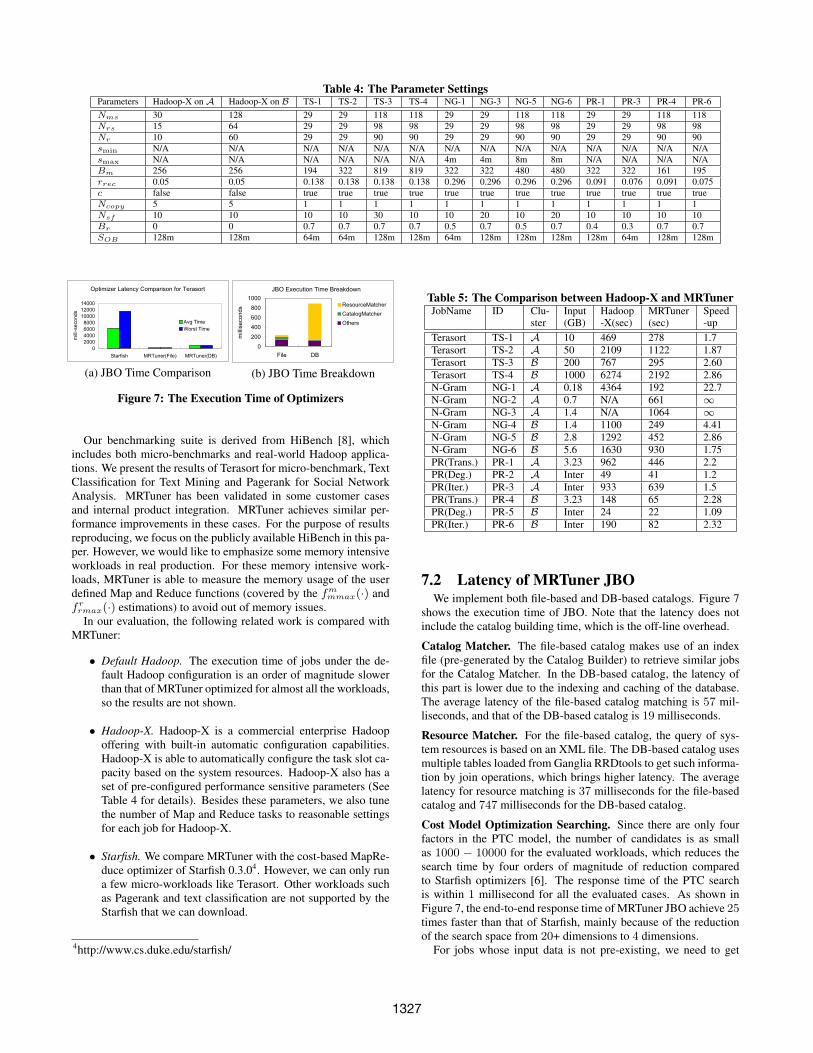
Table 4: The Parameter SettingsParameters Hadoop-X on A Hadoop-X on B TS-1 TS-2 TS-3 TS-4 NG-1 NG-3 NG-5 NG-6 PR-1 PR-3 PR-4 PR-6Nms 30 128 29 29 118 118 29 29 118 118 29 29 118 118Nrs 15 64 29 29 98 98 29 29 98 98 29 29 98 98Nr 10 60 29 29 90 90 29 29 90 90 29 29 90 90smin N/A N/A N/A N/A N/A N/A N/A N/A N/A N/A N/A N/A N/A N/Asmax N/A N/A N/A N/A N/A N/A 4m 4m 8m 8m N/A N/A N/A N/ABm 256 256 194 322 819 819 322 322 480 480 322 322 161 195rrec 0.05 0.05 0.138 0.138 0.138 0.138 0.296 0.296 0.296 0.296 0.091 0.076 0.091 0.075c false false true true true true true true true true true true true trueNcopy 5 5 1 1 1 1 1 1 1 1 1 1 1 1Nsf 10 10 10 10 30 10 10 20 10 20 10 10 10 10Br 0 0 0.7 0.7 0.7 0.7 0.5 0.7 0.5 0.7 0.4 0.3 0.7 0.7SOB 128m 128m 64m 64m 128m 128m 64m 128m 128m 128m 128m 64m 128m 128m

Optimizer Latency Comparison for Terasort

0

2000

4000

6000

8000

10000

12000

14000

Starfish MRTuner(File) MRTuner(DB)

milli-seconds

Avg Time

Worst Time

(a) JBO Time Comparison

JBO Execution Time Breakdown

0

200

400

600

800

1000

File DB

milliseconds ResourceMatcher

CatalogMatcher

Others

(b) JBO Time Breakdown

Figure 7: The Execution Time of Optimizers

Our benchmarking suite is derived from HiBench [8], whichincludes both micro-benchmarks and real-world Hadoop applica-tions. We present the results of Terasort for micro-benchmark, TextClassification for Text Mining and Pagerank for Social NetworkAnalysis. MRTuner has been validated in some customer casesand internal product integration. MRTuner achieves similar per-formance improvements in these cases. For the purpose of resultsreproducing, we focus on the publicly available HiBench in this pa-per. However, we would like to emphasize some memory intensiveworkloads in real production. For these memory intensive work-loads, MRTuner is able to measure the memory usage of the userdefined Map and Reduce functions (covered by the fm

mmax(·) andfrrmax(·) estimations) to avoid out of memory issues.

In our evaluation, the following related work is compared withMRTuner:

• Default Hadoop. The execution time of jobs under the de-fault Hadoop configuration is an order of magnitude slowerthan that of MRTuner optimized for almost all the workloads,so the results are not shown.

• Hadoop-X. Hadoop-X is a commercial enterprise Hadoopoffering with built-in automatic configuration capabilities.Hadoop-X is able to automatically configure the task slot ca-pacity based on the system resources. Hadoop-X also has aset of pre-configured performance sensitive parameters (SeeTable 4 for details). Besides these parameters, we also tunethe number of Map and Reduce tasks to reasonable settingsfor each job for Hadoop-X.

• Starfish. We compare MRTuner with the cost-based MapRe-duce optimizer of Starfish 0.3.04. However, we can only runa few micro-workloads like Terasort. Other workloads suchas Pagerank and text classification are not supported by theStarfish that we can download.

4http://www.cs.duke.edu/starfish/

Table 5: The Comparison between Hadoop-X and MRTunerJobName ID Clu- Input Hadoop MRTuner Speed

ster (GB) -X(sec) (sec) -upTerasort TS-1 A 10 469 278 1.7Terasort TS-2 A 50 2109 1122 1.87Terasort TS-3 B 200 767 295 2.60Terasort TS-4 B 1000 6274 2192 2.86N-Gram NG-1 A 0.18 4364 192 22.7N-Gram NG-2 A 0.7 N/A 661 ∞N-Gram NG-3 A 1.4 N/A 1064 ∞N-Gram NG-4 B 1.4 1100 249 4.41N-Gram NG-5 B 2.8 1292 452 2.86N-Gram NG-6 B 5.6 1630 930 1.75PR(Trans.) PR-1 A 3.23 962 446 2.2PR(Deg.) PR-2 A Inter 49 41 1.2PR(Iter.) PR-3 A Inter 933 639 1.5PR(Trans.) PR-4 B 3.23 148 65 2.28PR(Deg.) PR-5 B Inter 24 22 1.09PR(Iter.) PR-6 B Inter 190 82 2.32

7.2 Latency of MRTuner JBOWe implement both file-based and DB-based catalogs. Figure 7

shows the execution time of JBO. Note that the latency does notinclude the catalog building time, which is the off-line overhead.

Catalog Matcher. The file-based catalog makes use of an indexfile (pre-generated by the Catalog Builder) to retrieve similar jobsfor the Catalog Matcher. In the DB-based catalog, the latency ofthis part is lower due to the indexing and caching of the database.The average latency of the file-based catalog matching is 57 mil-liseconds, and that of the DB-based catalog is 19 milliseconds.

Resource Matcher. For the file-based catalog, the query of sys-tem resources is based on an XML file. The DB-based catalog usesmultiple tables loaded from Ganglia RRDtools to get such informa-tion by join operations, which brings higher latency. The averagelatency for resource matching is 37 milliseconds for the file-basedcatalog and 747 milliseconds for the DB-based catalog.

Cost Model Optimization Searching. Since there are only fourfactors in the PTC model, the number of candidates is as smallas 1000 − 10000 for the evaluated workloads, which reduces thesearch time by four orders of magnitude of reduction comparedto Starfish optimizers [6]. The response time of the PTC searchis within 1 millisecond for all the evaluated cases. As shown inFigure 7, the end-to-end response time of MRTuner JBO achieve 25times faster than that of Starfish, mainly because of the reductionof the search space from 20+ dimensions to 4 dimensions.

For jobs whose input data is not pre-existing, we need to get

1327

MapInputSplit (m)

MapOutputBuffer

MapOutputCompression (c)

ReduceCopy (v)

ReduceInputBuffer

ReduceOutput (r)

(a) TS-3

MapInputSplit (m)

MapOutputBuffer

MapOutputCompression (c)

ReduceCopy (v)

ReduceInputBuffer

ReduceOutput (r)

(b) NG-5

MapInputSplit (m)

MapOutputBuffer

MapOutputCompression (c)

ReduceCopy (v)

ReduceInputBuffer

ReduceOutput (r)

(c) PR-4

Figure 6: Impact of Parameter Groups on Selected Jobs

Disk Utilization

0%20%40%60%80%100%

0 135 270 405 540 675Running Time (sec)

Percentage

CPU Utilization

0%

20%

40%

60%

80%

100%

0 135 270 405 540 675Running Time (sec)

Utilization

wiosystemuser

Memory Used

020406080100120

0 135 270 405 540 675Running Time (sec)

GB

Network I/O

0

200

400

600

0 135 270 405 540 675Running Time (sec)

MB

bytes_in

bytes_out

(a) Hadoop-X

Disk Utilization

0%20%40%60%80%100%

0 60 120 180 240 300 360Running Time (sec)

Percentage

CPU Utilization

0%20%40%60%80%100%

0 60 120 180 240 300 360Running Time (sec)

Utilization

wiosystemuser

Memory Used

0

60

120

180

240

0 60 120 180 240 300 360Running Time (sec)

GB

Network I/O

0

100

200

300

0 60 120 180 240 300 360Running Time (sec)

MB

bytes_in

bytes_out

(b) MRTuner

Figure 8: Resource Utilization of TS-3

its data catalog on the fly, which leads to about 650 millisecondslatency. In such cases, we only use the data size and block sizeproperties of the data, and MRTuner still performs a factor of 6faster than Starfish on the job optimizer response time.

7.3 MRTuner EffectivenessTo evaluate the effectiveness of MRTuner, we show not only the

running time, but also system resource utilization, and elaboratewhy MRTuner outperforms the state-of-the-art MapReduce opti-mizer, especially focusing on the inter-task optimizations of thePTC model. For typical workloads, we give the quantitative analy-sis on how each of the parameter (group) affects the performance.Both Hadoop-X and MRTuner optimized settings are shown in Ta-ble 4. The running time of these workloads is listed in Table 5.Terasort. Terasort is a standard benchmark created by Jim Gray [12].The input data is generated by the TeraGen program. The elapsedtime of Terasort is shown in Table 5. MRTuner achieves the jobelapsed time of 2 and 3 times faster than Hadoop-X on cluster Aand B, respectively. Figure 8 and Figure 9 shows cluster-wide sys-tem resource utilization of TS-3 (200 GB) and TS-4 (1 TB) re-spectively. The figures indicate that MRTuner achieves much betterCPU utilization, less context switch overhead (indicated by the sys-tem CPU time), better memory utilization and less network over-head compared with Hadoop-X.

We analyze the impact of each parameter group for TS-3 in Fig-ure 6 (a) (See Table 3 for parameter groups). The ratio in Figure 6

Disk Utilization

0%20%40%60%80%100%

0 1440 2880 4320 5760Running Time (sec)

Percentage

CPU Utilization

0%20%40%60%80%100%

0 1440 2880 4320 5760Running Time (sec)

Utilization

wiosystemuser

Memory Used

0

60

120

180

0 1440 2880 4320 5760Running Time (sec)

GB

Network I/O

0

100

200

300

400

0 1440 2880 4320 5760Running Time (sec)

MB

bytes_in

bytes_out

(a) Hadoop-X

Disk Utilization

0%20%40%60%80%100%

0 450 900 1350 1800 2250Running Time (sec)

Percentage

CPU Utilization

0%20%40%60%80%100%

0 450 900 1350 1800 2250Running Time (sec)

Utilization

wiosystemuser

Memory Used

0

60

120

180

0 450 900 1350 1800 2250Running Time (sec)

GB

Network I/O

0

100

200

300

400

0 450 900 1350 1800 2250Running Time (sec)

MB

bytes_in

bytes_out

(b) MRTuner

Figure 9: Resource Utilization of TS-4

is obtained by setting the related parameters to the Hadoop-X set-ting. For example, to evaluate the impact of Map output buffergroup, we change related parameters from the MRTuner setting tothe Hadoop-X setting (i.e. Bm = 256 and rrec = 0.05) to get therunning time t′. Suppose that the job elapsed time of MRTuner ist. The impact of this parameter group is measured as t′−t

t. Finally,

we normalize all the ratio of impacts in a pie chart. Figure 6 (a)indicates that the Map output compression, the Map output bufferand the Reduce output are the top three influencing factors for theworkload TS-3.

Next we dissect optimizations on TS-3 to elaborate why MR-Tuner outperforms Hadoop-X. First, the task slot optimization ofMRTuner considers cluster-wide system resources. The non-linearprogramming model in Section 5.3 figures out the optimal configu-ration. The main contribution of this optimization is on the Reduceoutput. The increased parallelism improves 21.2% of the elapsedtime compared with Hadoop-X. Second, based on the estimationof map output properties (i.e. the size and the number of records),MRTuner ensures that there is no additional disk spills before Maptasks finish, which improves the job elapsed time by 26.99% overHadoop-X. (The disk read and write size of Hadoop-X is a factor of2.99 more than that of MRTuner, due to the additional spills.) Simi-larly, based on the estimation of Reduce input properties, MRTuneris able to allocate 70% of the JVM heap as the Reduce input buffer,which improves the job elapsed time by 6.27% over Hadoop-X.Third, the PTC model of MRTuner ensures the maximal overlap-

1328

Disk Utilization

0%20%40%60%80%

100%

0 180 360 540 720 900 1080 1260Running Time (sec)

Perc

enta

ge

CPU Utilization

0%20%40%60%80%

100%

0 180 360 540 720 900 1080 1260Running Time (sec)

Utiliz

ation

wiosystemuser

Memory Used

0

60

120

0 180 360 540 720 900 1080 1260Running Time (sec)

GB

Network I/O

0

200

400

600

0 180 360 540 720 900 1080 1260Running Time (sec)

MB

bytes_in

bytes_out

(a) Hadoop-X

Disk Utilization

0%20%40%60%80%100%

0 75 150 225 300 375 450Running Time (sec)

Percentage

CPU Utilization

0%20%40%60%80%100%

0 75 150 225 300 375 450Running Time (sec)

Utilization

wiosystemuser

Memory Used

020406080100120140160

0 75 150 225 300 375 450Running Time (sec)

GB

Network I/O

0

50

100

150

200

0 75 150 225 300 375 450Running Time (sec)

MB

bytes_in

bytes_out

(b) MRTuner

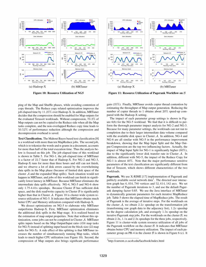
Figure 10: Resource Utilization of NG5

ping of the Map and Shuffle phases, while avoiding contention ofcopy threads. The Reduce copy related optimization improves thejob elapsed time by 11.25% over Hadoop-X. In addition, MRTunerdecides that the compression should be enabled for Map outputs forthe evaluated Terasort workloads. Without compression, 70.3% ofMap outputs can not be copied to the Reduce side when all the Maptasks complete, and the non-overlapped Reduce copy time leads to50.52% of performance reduction although the compression anddecompression overhead is saved.

Text Classification. The Mahout Bayes based text classification [8]is a workload with more than ten MapReduce jobs. The second job,which is to tokenize the words and n-grams in a document, accountsfor more than half of the total execution time. Thus the analysis be-low is focused on this job. The job elapsed time of this workloadis shown in Table 5. For NG-1, the job elapsed time of MRTuneris a factor of 22.7 faster that of Hadoop-X. For NG-2 and NG-3,Hadoop-X runs for more than three hours and still can not finish,and we observe a lot of disk errors caused by the overwhelmingdata spills in the Map phase (because of limited disk space of thecluster A and the expanded Map spills). Such situation would nothappen in MRTuner, and jobs of this workload can finish in signifi-cantly lower latency in MRTuner. Because MRTuner eliminates theintermediate data spills effectively. NG-4, NG-5 and NG-6 showonly 1.75-4.41x speedups. Because Cluster B has sufficient diskspace, and the disk read/write capacity in Cluster B is significantlyhigher than that in Cluster A. Figure 10 is cluster-wide system re-source utilization of NG-5. It indicates that MRTuner obtains muchbetter CPU and Memory utilization compared with Hadoop-X.

We dissect optimizations on NG-5 to elaborate why MRTuneroutperforms Hadoop-X. First, MRTuner optimization eliminatesthe additional disk spills in the Map stage. It is realized based onthe estimation of map output properties. Note that without this op-timization, some jobs can not be completed in Cluster A. MRTunersplits inputs based on the Map Output/Input ratio (456 map tasksfor NG-5) instead of splitting input based on the block size (22 maptasks for NG-5). A side effect of this splitting is that MRTuner in-creases the number of simultaneously running Map tasks, whichleads to much higher CPU utilization (see Figure 10). Second, thecompression of Map outputs also brings significant performance

Disk Utilization

0%20%40%60%80%100%

0 135 270 405 540 675 810Running Time (sec)

Percentage

CPU Utilization

0%

20%

40%

60%

80%

100%

0 135 270 405 540 675 810Running Time (sec)

Utilization

wiosystemuser

Memory Used

0

20

40

60

0 135 270 405 540 675 810Running Time (sec)

GB

Network I/O

0

100

200

300

0 135 270 405 540 675 810Running Time (sec)

MB

bytes_in

bytes_out

(a) Hadoop-X

Disk Utilization

0%20%40%60%80%100%

0 75 150 225 300 375Running Time (sec)

Percentage

CPU Utilization

0%20%40%60%80%100%

0 75 150 225 300 375Running Time (sec)

Utilization

systemwiouser

Memory Used

0

20

40

60

0 75 150 225 300 375Running Time (sec)

GB

Network I/O

0

100

200

300

0 75 150 225 300 375Running Time (sec)

MB

bytes_in

bytes_out

(b) MRTuner

Figure 11: Resource Utilization of Pagerank Workflow on B

gain (35%). Finally, MRTuner avoids copier thread contention byestimating the throughput of Map output generation. Reducing thenumber of copier threads to 1 obtains about 20% speed-up com-pared with the Hadoop-X setting.

The impact of each parameter group settings is shown in Fig-ure 6(b) for the NG-5 workload. We find that it is difficult to per-form the thorough parameter impact analysis for NG-2 and NG-3.Because for many parameter settings, the workloads can not run tocompletion due to their larger intermediate data volume comparedwith the available disk space in Cluster A. In addition, NG-4 andNG-6 are all similar with NG-5 in the performance improvementbreakdown, showing that the Map Input Split and the Map Out-put Compression are the top two influencing factors. Actually, theimpact of Map Input Split for NG-1 is significantly higher (80%),due to the significantly lower disk transfer rate in Cluster A. Inaddition, different with NG-5, the impact of the Reduce Copy forNG-1 is almost 40%. Note that the major performance sensitiveparameters of the text classification are significantly different fromthat of Terasort, which shows different characteristics of the twoworkloads.

Pagerank. We use X-RIME [17] implementation of Pagerank andpublicly available social network data5. The directed user interac-tion graph has 6, 034, 780 vertices and 52, 614, 182 arcs. We setthe number of Pagerank iterations to 3, and use the default Pager-ank damping factor 0.85. We use the Java interface of MRTunerto dynamically generate parameters for each iterative MapReducejob. Table 5 shows the elapsed time of MapReduce jobs. The resultof Pagerank is the average of iterative steps. For the workloads onthe cluster A, we obtain 2.2x speedup on the transformation job(transforming raw graph data to the adjacency list), 1.2x speedupon the degree calculation job, and averagely 1.5x speedup on theiterative Pagerank step jobs. For the workloads on the cluster B, weobtain 2.3x, 1.1x and 2.3x speedups for the three jobs, respectively.Figure 11 is cluster-wide system resource utilization of all jobs ofthe Pagerank workflow on the cluster B. It indicates that MRTunerobtains better CPU and memory utilization. The impact of each pa-rameter group on PR-4 in the cluster B is shown in Figure 6 (c). It

5http://current.cs.ucsb.edu/facebook/index.html

1329

indicates that the Reduce output, the Map output compression andthe Reduce copy are the top three influencing factors for PR-4.

Figure 11 (b) further indicates that the Reduce phases of bothPR-4 and PR-6 have downward trends in terms of CPU utilization.Through profiling Reduce tasks, we find that it is caused by dataskew [9]. The replication in HDFS writing further amplifies theimpact of data skew.

Although the skew issue is hardly to be addressed by parametertuning, it will affect the PTC model. For example, skew of Maptasks may increase the overlapped time duration for the Shufflestage. As future work, we are extending the PTC model to esti-mate task skew based on the historical task execution time.

Disk Utilization

0%20%40%60%80%100%

0 375 750 1125 1500 1875 2250Running Time (sec)

Percentage

CPU Utilization

0%20%40%60%80%100%

0 375 750 1125 1500 1875 2250Running Time (sec)

Utilization

wiosystemuser

Memory Used

0

20

0 375 750 1125 1500 1875 2250Running Time (sec)

GB

Network I/O

0

20

40

60

0 375 750 1125 1500 1875 2250Running Time (sec)

MB

bytes_in

bytes_out

(a) Starfish

Disk Utilization

0%20%40%60%80%

100%

0 188 377 565 753 942 1130Running Time (sec)

Perc

enta

ge

CPU Utilization

0%20%40%60%80%

100%

0 188 377 565 753 942 1130Running Time (sec)

Utiliz

ation

wiosystemuser

Memory Used

0

20

40

0 188 377 565 753 942 1130Running Time (sec)

GB

Network I/O

0

10

20

30

40

0 188 377 565 753 942 1130Running Time (sec)

MB

bytes_in

bytes_out

(b) MRTuner

Figure 12: Resource Utilization of TS2

7.4 Comparison with StarfishWe deploy Starfish 0.3.0 in the cluster A, but fail to configure

it in the cluster B due to JVM issues. Since the version which wedownload only supports a few micro-workloads such as Terasortand Word Count, we only compare these workloads that are avail-able in Starfish. The latency of JBO is compared in Section 7.2.

We present the effectiveness of job optimizers. For TS-2, thejob elapsed time of MRTuner is a factor of 1.6 faster than that ofStarfish. Figure 12 shows system resource utilization of Starfishand MRTuner on TS-2, which indicates that MRTuner has bettersystem resource utilization. When we compare the suggested exe-cution plans, we find that more network I/O of MRTuner are over-lapped with the Map stage. Also, there is no additional disk I/Oin Map outputs using the MRTuner generated parameters for TS-2.Finally, there is much less context switch overhead since the PTCmodel optimizes tasks among Map and Reduce stages.

8. CONCLUSIONIn this paper, we proposed the MRTuner toolkit to enable holis-

tic optimization for MapReduce jobs. The Producer-Transporter-Consumer model was proposed to estimate the tradeoffs in MapRe-duce execution plans. The relationship among parameters was de-rived to develop a fast search algorithm. The experimental eval-uation based on HiBench demonstrated the effectiveness and effi-ciency of MRTuner. As future work, we are extending the PTCmodel in YARN to address the multi-tenancy and skew issues.

9. ACKNOWLEDGMENTSThe authors would like to thank Ning Yang, Zeli Liu and Zelin

An from RUC, and Zhongxin Guo from BUPT, for implementingthe initial prototype of the catalog. The authors also thank anony-mous reviewers for their valuable comments and suggestions to im-prove the paper. Jiaheng Lu is partially supported by NSF China(No. 60903056), 863 National High-tech Research Plan of China(No. 2012AA011001), IBM-RUC research funds and the Funda-mental Research Fund for RUC.

10. REFERENCES[1] S. Chaudhuri. An overview of query optimization in

relational systems. In PODS, pages 34–43, 1998.[2] S. Chaudhuri. What next?: a half-dozen data management

research goals for big data and the cloud. In PODS, pages1–4, 2012.

[3] D. Culler, R. Karp, D. Patterson, A. Sahay, K. E. Schauser,E. Santos, R. Subramonian, and T. von Eicken. Logp:Towards a realistic model of parallel computation. SIGPLANNot., 28(7):1–12, 1993.

[4] A. J. Elmore, S. Das, A. Pucher, D. Agrawal, A. El Abbadi,and X. Yan. Characterizing tenant behavior for placementand crisis mitigation in multitenant dbmss. In SIGMOD,pages 517–528, 2013.

[5] L. Grit, D. Irwin, A. Yumerefendi, and J. Chase. Virtualmachine hosting for networked clusters: Building thefoundations for ”autonomic” orchestration. In VTDC, page 7,2006.

[6] H. Herodotou and S. Babu. Profiling, what-if analysis, andcost-based optimization of mapreduce programs. PVLDB,4(11):1111–1122, 2011.

[7] H. Herodotou, H. Lim, G. Luo, N. Borisov, L. Dong, F. B.Cetin, and S. Babu. Starfish: A self-tuning system for bigdata analytics. In CIDR, pages 261–272, 2011.

[8] S. Huang, J. Huang, J. Dai, T. Xie, and B. Huang. Thehibench benchmark suite: Characterization of themapreduce-based data analysis. In ICDEW, pages 41–51,2010.

[9] Y. Kwon, M. Balazinska, B. Howe, and J. Rolia. Skewtune:Mitigating skew in mapreduce applications. In SIGMOD,pages 25–36, 2012.

[10] J. K. Laurila, D. Gatica-Perez, I. Aad, O. Bornet, T.-M.-T.Do, O. Dousse, J. Eberle, and M. Miettinen. The mobile datachallenge: Big data for mobile computing research. In Proc.of Nokia Mobile Data Challenge Workshop, 2012.

[11] B. Li, E. Mazur, Y. Diao, A. McGregor, and P. Shenoy. Aplatform for scalable one-pass analytics using mapreduce. InSIGMOD, pages 985–996, 2011.

[12] O. OMalley and A. C. Murthy. Winning a 60 second dashwith a yellow elephant. Sort Benchmark, 2009.

[13] N. Park, I. Ahmad, and D. J. Lilja. Romano: autonomousstorage management using performance prediction inmulti-tenant datacenters. In SoCC, pages 1–14, 2012.

[14] L. G. Valiant. A bridging model for parallel computation.Commun. ACM, 33(8):103–111, 1990.

[15] G. Wang, A. R. Butt, P. Pandey, and K. Gupta. A simulationapproach to evaluating design decisions in mapreduce setups.In MASCOTS, pages 1–11, 2009.

[16] T. White. Hadoop: The Definitive Guide. O’Reilly, 2012.[17] W. Xue, J. Shi, and B. Yang. X-rime: cloud-based large scale

social network analysis. In SCC, pages 506–513, 2010.

1330