mrt methodology & rapid code system · time simulation of an spect device for generation of...
TRANSCRIPT

MRT Methodology & RAPID Code SystemAlireza Haghighat
Professor and DirectorNuclear Engineering Program
Mechanical Engineering DepartmentVirginia TechArlington, VA
https://nuclear.ncr.vt.edu
(August 2018)

2
Particle Transport Theory & the MRT Methodology

Neutronics Simulation Approaches• Deterministic Methods
• Solve the linear Boltzmann equation to obtain the expected flux in a phase space
where, 𝐻 = 𝛺 ∙ 𝛻 + 𝜎 𝑟, 𝐸 − ∫ 𝑑𝐸′∫ 𝑑𝛺′𝜎𝑠( 𝑟, 𝐸′ → 𝐸, 𝛺′ ∙ 𝛺),
𝐹 = ∫ 𝑑𝐸′∫ 𝑑𝛺′𝜈𝜎𝑓 𝑟, 𝐸′ ,
𝜓 = 𝜓 𝑟, 𝐸, Ω , 𝑎𝑛𝑑 𝑆𝑖𝑛𝑑 = 𝑆𝑖𝑛𝑑 𝑟, 𝐸, Ω
• Statistical Monte Carlo Methods• Perform particle transport experiments using random numbers
(RN’s) and pdf’s on a computer to estimate average number of particles in phase space and associated uncertainty
3
Tally (count)
S (r, E, Ω) Sample • Small relative statistical
uncertainty, 𝑆 𝑥
𝑥
• Variance reduction techniques are needed
Book: Alireza Haghighat on Monte Carlo Methods for Particle Transport, published by CRC Press, Taylor & Francis Group, 2014

My JourneyParticle Transport Algorithms Development
4
Year
2019
2018
2017
2016
2015
2013
2009
2007
2005
1997
1996
1992
1989
1986
Methodology
MRT
MRT
VRS-MRT
MRT
MRT
MRT
MRT
Hybrid MC-det. (AVR)
Hybrid det. – det.
Hybrid MC-det. (automated VR - AVR)
Parallel (3-D)
Vector & parallel (2-D)
Parallel processing (1-D)
Vector processing (1-D)
Computer code system
tRAPID
bRAPID
VRS-RAPID
RAPID
TITAN-IR
AIMS
INSPCT-s
ADIES (𝑒−)
TITAN (n, ϒ)
A3MCNP (n, ϒ)
PENTRAN (n, ϒ)
Wall clock time
A few processors
100’s –1000’s cores
1 core
Former & Current Students
V. Mascolino
N. Roskoff
V. Mascolino
Dr. Walters & N. Roskoff
Dr. Royston
Drs. Royston & W. Walters
Dr. W. Walters
Dr. B. Dionne
Dr. C. Yi & Dr. W. Walters
Dr. J. Wagner, Dr. D. Shedlock
Dr. G. Sjoden, Dr. V. Kucukboyaci
Drs. M. Hunter, R. Mattis& B. Petrovic

Development of Particle Transport Formulations and Methodologies for Real-Time Calculations
• Physics-Based transport methodologies are needed:
• Based on problem physics partition a problem into stages (sub-problems),
• For each stage employ response method and/or adjoint function methodology
• Pre-calculate response-function or adjoint-function using an accurate and fast transport code
• Solve a linear system of equations to couple all the stages in real-time
5
*Haghighat, A., K. Royston, and W. Walters, “MRT Methodologies for Real-Time Simulation of Nonproliferation and Safeguards Problems,” Annals of Nuclear Energy, pp. 61-67, 2015.

Application of the • Nondestructive testing: Optimization of the Westinghouse’s PGNNA active interrogation
system for detection of RCRA (Resource Conversation and Recovery Act) (e.g., lead, mercury, cadmium) in waste drums (partial implementation of MRT; 1999)1
• Nuclear Safeguards: Monitoring of spent fuel pools for detection of fuel diversion (funded by LLNL); Developed INSPCT-s code system (2007)2
• Nuclear nonproliferation: Active interrogation of cargo containers for simulation of special nuclear materials (SNMs) (2013) (in collaboration with GaTech); developed the AIMS (Active Interrogation for Monitoring Special-nuclear-materials) code system (2013)3,4
• Image reconstruction for SPECT (Single Photon Emission Computed Tomography): Real-time simulation of an SPECT device for generation of project images using an MRT methodology and Maximum Likelihood Estimation Maximization (MLEM); Developed the TITAN-IR code system (filed for a patent, June 2015)5,6
6

Select references MRT Algorithms
1) B. Petrovic, A. Haghighat, A. Dulloo, and T. G. Congedo, “Hybrid Forward Monte-Carlo - Adjoint Sn Methodology for Simulation of PGNAA Systems, “ Proceedings of the Mathematics and Computation, Reactor Physics and Environmental Analysis in Nuclear Applications, Vol. 2, 1016-1025, Madrid, Spain, Sept. 27-30, 1999.
2) Walters, W., A. Haghighat, S. Sitaraman, and Y. Ham, “Development of INSPCT-S for Inspection of Spent Fuel Pool,” Journal of ASTM International, American Institute of Physics, NY, Volume 9, Issue 4, 2012.
3) Royston, K., A. Haghighat, W. Walters, C. Yi and G. Sjoden, Determination of Angular Current at a Detector Window Using a Hybrid Adjoint Function Methodology, Progress in Nuclear Science and Technology, Volume 4, pp. 528-532, April 2014.
4) Walters, W., A. Haghighat, K. Royston, C. Yi, and G. Sjoden, A Response Function Methodology to Calculate Induced Fission Neutron Flux Distribution in an Active Interrogation System, Progress in Nuclear Science and Technology, Volume 4, pp. 533-537, April 2014.
5) Royston, K. and A. Haghighat, “Preliminary Results of a New Deterministic Iterative Image Reconstruction Algorithm,” Proc. ANS RPSD 2014, Knoxville, TN, September 14-18, 2014.
6) Haghighat, A., K. Royston, G. Sjoden, C. Yi, and M. Huang, Unique Formulations in TITAN and PENTRAN for Medical Physics Applications, Progress in Nuclear Science and Technology, Volume 4, pp. 883-887, 2014.
7
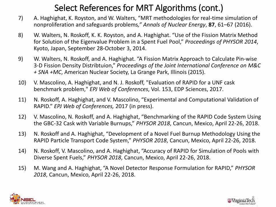
Select References for MRT Algorithms (cont.)7) A. Haghighat, K. Royston, and W. Walters, “MRT methodologies for real-time simulation of
nonproliferation and safeguards problems,” Annals of Nuclear Energy, 87, 61–67 (2016).
8) W. Walters, N. Roskoff, K. K. Royston, and A. Haghighat. “Use of the Fission Matrix Method for Solution of the Eigenvalue Problem in a Spent Fuel Pool,” Proceedings of PHYSOR 2014, Kyoto, Japan, September 28-October 3, 2014.
9) W. Walters, N. Roskoff, and A. Haghighat. “A Fission Matrix Approach to Calculate Pin-wise 3-D Fission Density Distribtuion,” Proceedings of the Joint International Conference on M&C + SNA +MC, American Nuclear Society, La Grange Park, Illinois (2015).
10) V. Mascolino, A. Haghighat, and N. J. Roskoff, "Evaluation of RAPID for a UNF cask benchmark problem," EPJ Web of Conferences, Vol. 153, EDP Sciences, 2017.
11) N. Roskoff, A. Haghighat, and V. Mascolino, “Experimental and Computational Validation of RAPID.” EPJ Web of Conferences, 2017 (in press).
12) V. Mascolino, N. Roskoff, and A. Haghighat, “Benchmarking of the RAPID Code System Using the GBC-32 Cask with Variable Burnups,” PHYSOR 2018, Cancun, Mexico, April 22-26, 2018.
13) N. Roskoff and A. Haghighat, “Development of a Novel Fuel Burnup Methodology Using the RAPID Particle Transport Code System,” PHYSOR 2018, Cancun, Mexico, April 22-26, 2018.
14) N. Roskoff, V. Mascolino, and A. Haghighat, “Accuracy of RAPID for Simulation of Pools with Diverse Spent Fuels,” PHYSOR 2018, Cancun, Mexico, April 22-26, 2018.
15) M. Wang and A. Haghighat, “A Novel Detector Response Formulation for RAPID,” PHYSOR 2018, Cancun, Mexico, April 22-26, 2018.
8

RAPID code system &VRS-RAPID
9

• Commonly used approach - MC Simulation
• Issues associated with MC:• Source Convergence in eigenvalue MC is difficult due to under
sampling (due to absorbers), HDR, cycle-to-cycle correlation• These effects are difficult to detect
• Computation times are very long, especially to get detailed information
• Changing system configuration (for design and analysis) requires complete recalculation
• Therefore, significant conservatism is introduced in the safety evaluations; this may introduce
• Difficulties in the licensing process • Limitations in the use of facilities• Difficulties during operation
Modeling of Nuclear Systems (cores, pools & casks)
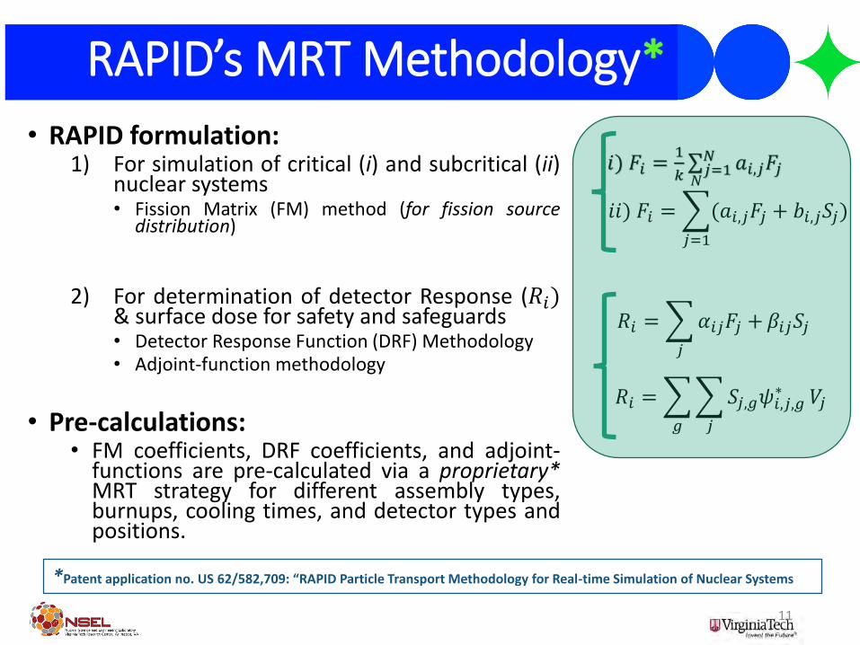
RAPID’s MRT Methodology*
• RAPID formulation:1) For simulation of critical (i) and subcritical (ii)
nuclear systems• Fission Matrix (FM) method (for fission source
distribution)
2) For determination of detector Response (𝑅𝑖)& surface dose for safety and safeguards• Detector Response Function (DRF) Methodology• Adjoint-function methodology
• Pre-calculations:• FM coefficients, DRF coefficients, and adjoint-
functions are pre-calculated via a proprietary*MRT strategy for different assembly types,burnups, cooling times, and detector types andpositions.
11
*Patent application no. US 62/582,709: “RAPID Particle Transport Methodology for Real-time Simulation of Nuclear Systems
𝑖) 𝐹𝑖 =1
𝑘 𝑗=1𝑁 𝑎𝑖,𝑗𝐹𝑗
𝑖𝑖) 𝐹𝑖 =
𝑗=1
𝑁
(𝑎𝑖,𝑗𝐹𝑗 + 𝑏𝑖,𝑗𝑆𝑗)
𝑅𝑖 =
𝑗
𝛼𝑖𝑗𝐹𝑗 +𝛽𝑖𝑗𝑆𝑗
𝑅𝑖 =
𝑔
𝑗
𝑆𝑗,𝑔𝜓𝑖,𝑗,𝑔∗ 𝑉𝑗
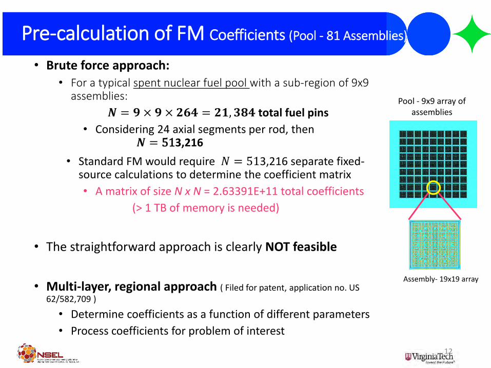
• Brute force approach:• For a typical spent nuclear fuel pool with a sub-region of 9x9
assemblies:
𝑵 = 𝟗 × 𝟗 × 𝟐𝟔𝟒 = 𝟐𝟏, 𝟑𝟖𝟒 total fuel pins
• Considering 24 axial segments per rod, then 𝑵 = 513,216
• Standard FM would require 𝑁 = 513,216 separate fixed-source calculations to determine the coefficient matrix
• A matrix of size N x N = 2.63391E+11 total coefficients
(> 1 TB of memory is needed)
• The straightforward approach is clearly NOT feasible
• Multi-layer, regional approach ( Filed for patent, application no. US 62/582,709 )
• Determine coefficients as a function of different parameters
• Process coefficients for problem of interest
Pool - 9x9 array of assemblies
12
Pre-calculation of FM Coefficients (Pool - 81 Assemblies)
Assembly- 19x19 array

13
RAPID Code System Flowchart
Pre-calculation using p3RAPID*
* p3RAPID: Pre- and Post-Processing module for RAPID

Simulation of Critical and Subcritical nuclear systems
Spent fuel pools, Spent fuel casks, and reactor cores
14

• Performed eigenvalue calculations for a 2x2 segment of the reference SFP.
• 4 test cases are defined, each containing different combinations of burnups/cooling times
• Fuel region of the model partitioned into 32,256 fission regions (tallies) (for 1344 pins with 24 axial levels)
• Reference MCNP eigenvalue parameters are:
• 106 particles per cycle, 400 skipped cycles 400 active cycles
15
Spent fuel pool - Test Cases
15
Burnup [GWd/MTHM]
Cooling Time [years*]
*’0 year’ cooling time refers to ~14 days
CASE 2 CASE 3 CASE 4
0 GWd/MTHM
0yr
37GWd/MTHM
0yr
37GWd/MTHM
0yr
0GWd/MTHM
0yr
0 GWd/MTHM
0yr
59GWd/MTHM
0yr
59GWd/MTHM
0yr
0GWd/MTHM
0yr
59 GWd/MTHM
9 yr
37GWd/MTHM
0yr
37GWd/MTHM
0yr
59GWd/MTHM
9yr
59 GWd/MTHM
9yr
37GWd/MTHM
9yr
37GWd/MTHM
9yr
59GWd/MTHM
9yr
CASE 1
16
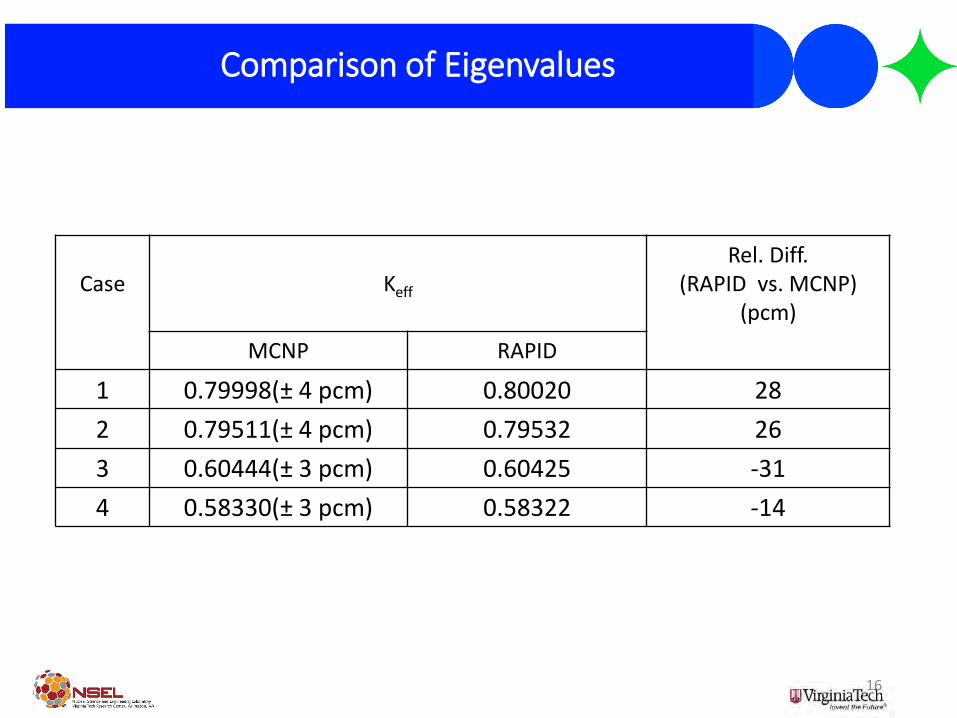
Comparison of Eigenvalues
Case Keff
Rel. Diff. (RAPID vs. MCNP)
(pcm)
MCNP RAPID
1 0.79998(± 4 pcm) 0.80020 28
2 0.79511(± 4 pcm) 0.79532 26
3 0.60444(± 3 pcm) 0.60425 -31
4 0.58330(± 3 pcm) 0.58322 -14

17
1-σ Relative UncertaintyFission Density
MCNP prediction – 3-D Fission Density (Case 1)
0 GWd/MTHM
0yr
37GWd/MTHM
0yr
37GWd/MTHM
0yr
0GWd/MTHM
0yr

18
RAPID MCNP % Relative Difference
0 GWd/MTHM
0yr
37GWd/MTHM
0yr
37GWd/MTHM
0yr
0GWd/MTHM
0yr
RAPID vs. MCNP – Fission Density (Case 1)

19
1-σ Relative Uncertainty
Fission Density
MCNP prediction – Fission Density (Cases 2-4)
Case 2 Case 3 Case 4

20
RAPID MCNP % Relative Difference
RAPID vs. MCNP – Fission Density (Case 2)
0 GWd/MTHM
0yr
59GWd/MTHM
0yr
59GWd/MTHM
0yr
0GWd/MTHM
0yr
21
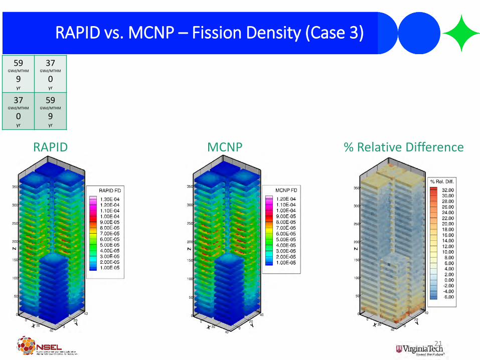
RAPID MCNP % Relative Difference
RAPID vs. MCNP – Fission Density (Case 3)
59 GWd/MTHM
9 yr
37GWd/MTHM
0yr
37GWd/MTHM
0yr
59GWd/MTHM
9yr

22
RAPID MCNP % Relative Difference
RAPID vs. MCNP – Fission Density (Case 4)
59 GWd/MTHM
9yr
37GWd/MTHM
9yr
37GWd/MTHM
9yr
59GWd/MTHM
9yr

23
Case
MCNP RAPID
CoresTime(min)
CoresTime (min)
Speedup
1 16 1020 (17 hrs) 1 0.50 2044
2 16 1013 (17 hrs) 1 0.51 1980
3 16 1082 (18 hrs) 1 0.50 2163
4 16 1149 (19 hrs) 1 0.50 2284
Computation Time
24
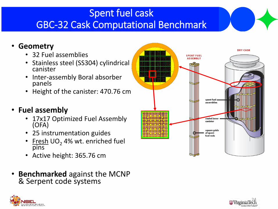
• Geometry• 32 Fuel assemblies• Stainless steel (SS304) cylindrical
canister• Inter-assembly Boral absorber
panels• Height of the canister: 470.76 cm
• Fuel assembly• 17x17 Optimized Fuel Assembly
(OFA)• 25 instrumentation guides• Fresh UO2 4% wt. enriched fuel
pins• Active height: 365.76 cm
• Benchmarked against the MCNP & Serpent code systems
Spent fuel caskGBC-32 Cask Computational Benchmark

# pins = 264; #axial levels = 24; # tallies = 6336
Case MCNP RAPID
𝒌𝒆𝒇𝒇 1.18030 (± 2 pcm) 1.18092
𝒌𝒆𝒇𝒇 relative difference - 53 pcm
Fiss. density adjusted rel. uncertainty
0.48% -
Fission density relative diff. - 0.65%
Computer 16 cores 1 core
Time666 min
(11.1 hours)0.1 min
(6 seconds)
Speedup - 6,666
RAPID vs. MCNP – Single assembly model

Case MCNP RAPID
𝒌𝒆𝒇𝒇 1.14545 (± 1 pcm) 1.14590
Relative Difference - 39 pcm
Fission density rel. uncertainty 1.15% -
Fission density relative diff. - 1.56%
Computer 16 cores 1 core
Time13,767 min(9.5 days)
0.585 min(35 seconds)
Speedup - 23,533
#assemblies = 32; # pins = 264; #axial levels = 24; # tallies = 202,752
RAPID vs. MCNP – FULL Cask model
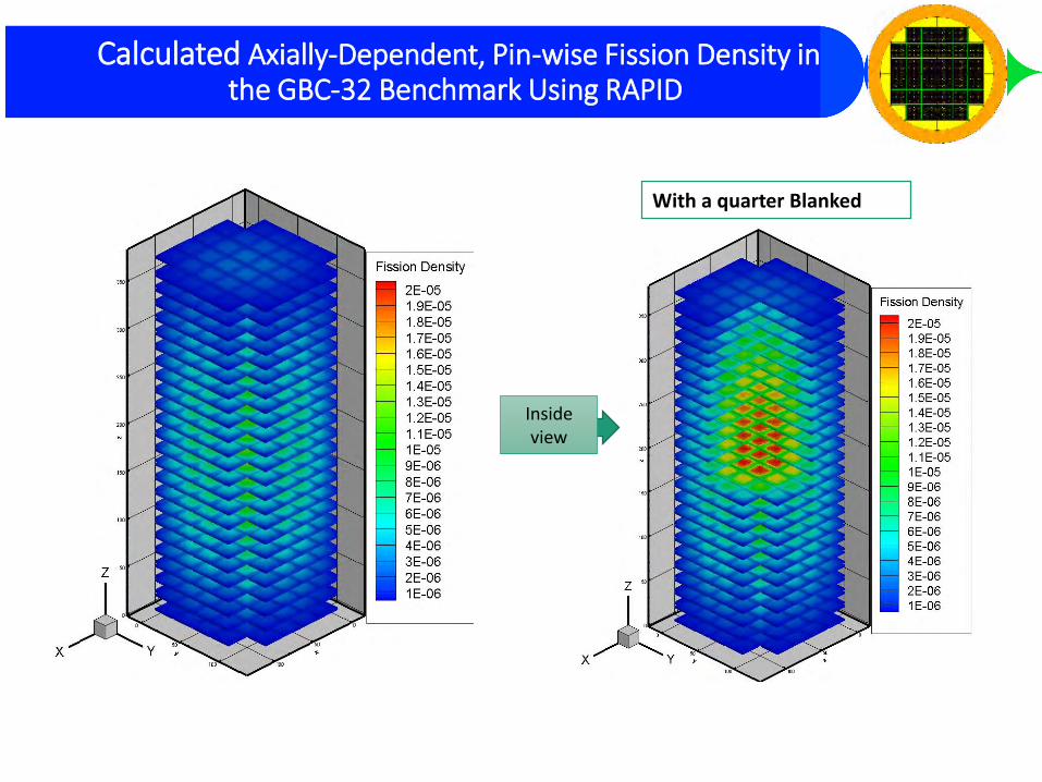
With a quarter Blanked
Inside view
Calculated Axially-Dependent, Pin-wise Fission Density in the GBC-32 Benchmark Using RAPID

#assemblies = 32; # pins = 264; #axial levels = 48; # tallies = 405,504
RAPID vs. Serpent – FULL Cask Variable Burnup
Burnup(MWd/MT)
Serpent(3σ)
RAPID Rel. Diff(pcm)
Fresh fuel 1.14546 ± 30 pcm 1.14545 -15,000 1.06602 ± 30 pcm 1.06607 510,000 1.02413 ± 33 pcm 1.02444 3120,000 0.93766 ± 33 pcm 0.93777 1130,000 0.84557 ± 33 pcm 0.84569 1240,000 0.75113 ± 33 pcm 0.75120 7
Comparison of keff for different CASK models with different burnups

#assemblies = 32; # pins = 264; #axial levels = 48; # tallies = 405,504
RAPID vs. Serpent – FULL Cask,Variable Burnup - Checkerboard Models
Comparison of keff for different checkerboard CASK models
Model Serpent (3σ ) RAPID Rel. Diff (PCM)
1 0.98679 ± 36 pcm 0.98693 14
2 1.03336 ± 33 pcm 1.03343 7
3 1.05311 ± 33 pcm 1.05336 25

RAPID: #assemblies = 32; # pins = 264; #axial levels = 48; # tallies = 405,504
RAPID vs. Serpent – FULL Cask,Computation Time
Serpent: only 12 axial levels, and fission source uncertainty may be large

RAPID vs. SERPENTReactor Core
31

*W. Walters, N. Roskoff, and A. Haghighat, ”The RAPID Fission Matrix Approach to Reactor CoreCriticality Calculations,” Accepted for publication in the Journal Nuclear Science and Engineering (June, 2018)
• RAPID has been applied to several large PWR problems, based on the NEA/OECD Monte Carlo Performance Benchmark Problem.
• 241 assemblies; 17x17 lattice; 264 fuel pins + 25 control/instrumentation tubes per assembly; 24 GWd/MT+ chemical shim
• 100 axial levels
• 6.4 million cells
• FM coefficients are pre-calculated using the SERPENT Monte Carlo code for different core configurations
32
Reactor Core - RAPID vs. SERPENT – PWR*
RPV
Downcomer
Baffle plates & core barrel mixture

33
Sample ResultRAPID vs. SERPENT – Keff & Compuation Time
Method Keff Relative Diff
Serpent 1.000855 ±1.0 𝑝𝑐𝑚 -
RAPID 1.000912 ±1.4 𝑝𝑐𝑚 5.3 pcm
Method # Cores CPU (hrs) Speedup
Serpent 20 1000 -
RAPID* 1 0.23 4348
*Pre-calculation requires about 700 CPU hrs

34
Sample ResultRAPID vs. SERPENT –Fission Density
Pin-wise Fission Source
X-Y reactor core layout.
RAPID-Serpent Difference Axial Fission density
Fission density along single pins
Type Serpent RAPID
RMS 2.03% 0.21%
Max 10.16%* 3.64%
*has not converged!
Pin-wise fission source
1-σ Uncertainty
RMS error : 2.18%

Experimental Benchmarking of RAPIDUS Naval Academy Subcritical Facility
35

• A cylindrical pool with natural uranium (fuel) and light water (moderator)
• There are a total of 268 fuel rods, arranged in a hexagonal lattice
• Fuel: hollow aluminum tubes containing 5 annular fuel slugs
• Neutron source: PuBe
03/10/16 12:03:23
c Original Assembly Burnup file
= sdir=xsdi
probid = 03/10/16 12:03:22
basis: XY
( 1.000000, 0.000000, 0.000000)
( 0.000000, 1.000000, 0.000000)
origin:
( 0.00, 0.00, -98.00)
extent = ( 61.50, 61.50)
03/10/16 12:03:22
c Original Assembly Burnup file
= sdir=xsdi
probid = 03/10/16 12:03:22
basis: XZ
( 1.000000, 0.000000, 0.000000)
( 0.000000, 0.000000, 1.000000)
origin:
( 0.00, 0.00, -49.00)
extent = ( 80.00, 80.00)
104.14 cm
17.78 cm
9.68 cm
154.2cm
R = 60.94 cm
36
Model Description - USNA-SC
03/10/16 12:03:23
c Original Assembly Burnup file
= sdir=xsdi
probid = 03/10/16 12:03:22
basis: XY
( 1.000000, 0.000000, 0.000000)
( 0.000000, 1.000000, 0.000000)
origin:
( 0.00, 0.00, -98.00)
extent = ( 61.50, 61.50)

Axial-Dependent (41 nodes), Pin-Wise Fission Density Distribution (10,988 tallies)
37
RAPID code system MCNP code systemRelative difference
(%)RAPID vs. MCNP
Code # Processors Time (min) Speedup
MCNP 8 819.5 (>13hrs) -RAPID 1 0.22 (13 s) 3774

38
𝜎𝑓 =𝜎𝑐2
𝑚2+𝑐2𝜎𝑚
2
𝑚4
Estimation of uncertainty in 𝑓 =𝐶
𝑚
Calculated C/E and Estimated Uncertainty
03/10/16 12:03:23
c Original Assembly Burnup file
= sdir=xsdi
probid = 03/10/16 12:03:22
basis: XY
( 1.000000, 0.000000, 0.000000)
( 0.000000, 1.000000, 0.000000)
origin:
( 0.00, 0.00, -98.00)
extent = ( 61.50, 61.50)
pins 101 & 102 (along z-axis)
external detectors (A & B)
Pins along 3 diagonals

RAPIDDetector Response or Surface Dose Calculation for
Monitoring, Safety & Safeguards
39

40
RAPID Code System Flowchart
Pre-calculation using p3RAPID*
* p3RAPID: Pre- and Post-Processing module for RAPID

• Detector Response Function (DRF) Methodology
Response at detector 𝑖 is calculated by
𝑅𝑖 =
𝑗
𝛼𝑖𝑗𝐹𝑗 +𝛽𝑖𝑗𝑆𝑗
Where, 𝐹𝑗and 𝑆𝑗 refer to fission and independent sources, respectively, and 𝛼𝑖𝑗and 𝛽𝑖𝑗refer to DRF coefficients, representing the normalized response of detector 𝑖 due fission and independent sources at position 𝑗, respectively.
41
Detector Response Function (DRF)
𝑅𝑖
• The detector field-of-view (FOV) is obtained based on the adjoint function methodology using the PENTRAN deterministic code system
• The DRF coefficients (𝜶𝒊𝒋, 𝜷𝒊𝒋) within the detector FOV are determined through a series of fixed-source Monte Carlo calculations using the CADIS variance reduction methodology
42
Pre-CalculationDetermination of DRF Coefficients
Automation: After determining the FOV, we have developed a software, DpRAPID, that automatically prepares input files for performing MCNP-CADIS calculations to obtain the DRF coefficients.

• Determination of a He-3 count rate placed on the surface of spent fuel cask
• GBC-32 (32 PWR assemblies; 17x17 lattice)• Burnup: 50 GWd/MT• Cooling time: 0.0 yr
• He-3 detector• Size = 2.5x2.5x10 cm3
• Pre-calculation• Using a PENTRAN model we determined the FOV of a He-3
detector.• The blue rectangles in the above figures show the radial and axial
extends of the FOV volume.
• Fixed-source MCNP-CADIS calculations were performed for each fuel pellet in every fuel pin with in the FOV volume
43
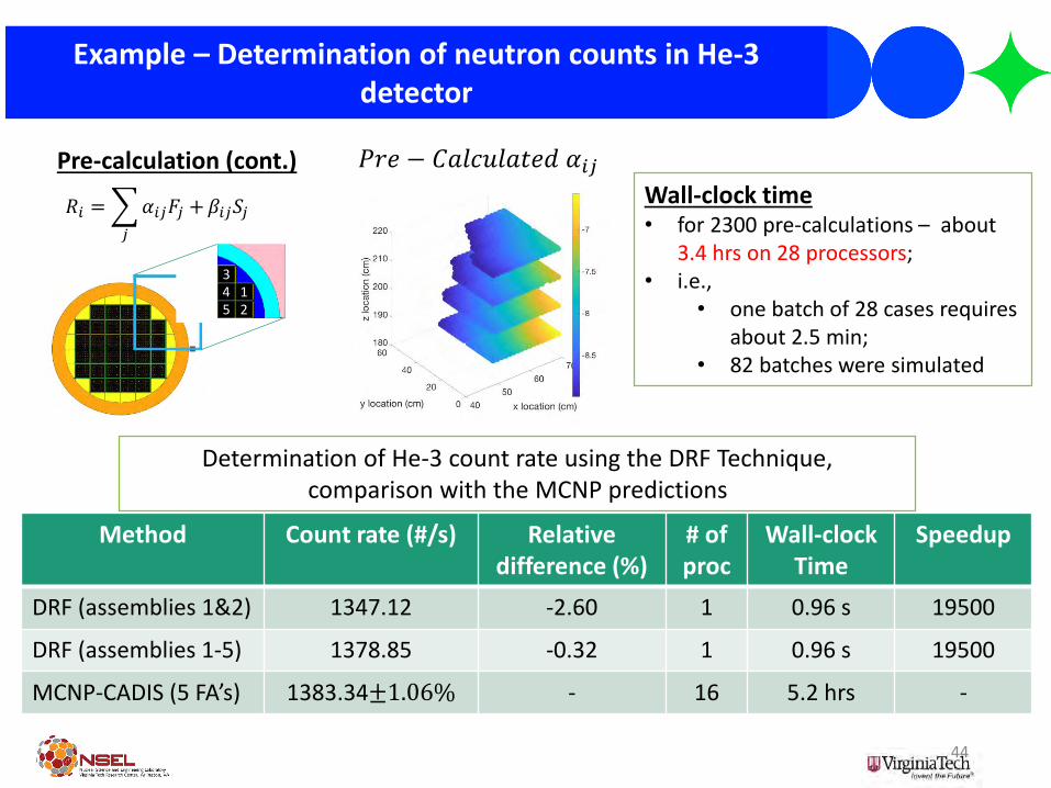
Example – Determination of neutron counts in He-3 detector
Schematic of GBC-32
44
Example – Determination of neutron counts in He-3 detector
𝑃𝑟𝑒 − 𝐶𝑎𝑙𝑐𝑢𝑙𝑎𝑡𝑒𝑑 𝛼𝑖𝑗Wall-clock time • for 2300 pre-calculations – about
3.4 hrs on 28 processors;• i.e.,
• one batch of 28 cases requires about 2.5 min;
• 82 batches were simulated
Method Count rate (#/s) Relativedifference (%)
# of proc
Wall-clock Time
Speedup
DRF (assemblies 1&2) 1347.12 -2.60 1 0.96 s 19500
DRF (assemblies 1-5) 1378.85 -0.32 1 0.96 s 19500
MCNP-CADIS (5 FA’s) 1383.34±1.06% - 16 5.2 hrs -
312
45
𝑅𝑖 =
𝑗
𝛼𝑖𝑗𝐹𝑗 +𝛽𝑖𝑗𝑆𝑗
Pre-calculation (cont.)
Determination of He-3 count rate using the DRF Technique, comparison with the MCNP predictions

Novel bRAPID Algorithm Compared with the standard algorithm
45
Standard Burnup Approach bRAPID’s Novel Algorithm

Burnup for RAPID - bRAPID: Algorithm
46

• Based on the OECD/NEA Monte Carlo Performance Benchmark*
• 241 Assemblies, 17x17 fuel lattice
Reference Model
47
Fuel Assembly
X-Y View X-Z View*Uniform moderator density & fresh fuel (4.0 wt%235U)

• 5x5 Mini Core w/ 4 axial zones• 84 burnable regions
• Burn this model with:• Power density = 25 kW/kg• Irradiation Time = 1 year (10 steps)• Total Burnup = 9,131 MWd/MTHM
3D Test Problem
48

3D Problem: Eigenvalues & Time
49
Method No. Proc. Time Speedup
Serpent 32 4.3 d --
bRAPID 1 21 min 294

3D Model: Fission Source & Mats
50

• Time-dependent flux equation (no external source):
1
𝑣⋅𝜕𝜓 𝑝, 𝑡
𝜕𝑡+ 𝜎𝑡 𝑝, 𝑡 𝜓 𝑝, 𝑡 + Ω ⋅ 𝛻𝜓 𝑝, 𝑡 − ∫ 𝑑𝑝′𝜎𝑠 𝑝′ → 𝑝 𝜓 𝑝′, 𝑡 =
1 − 𝛽𝜒𝑝 𝐸
4𝜋∫ 𝑑𝑝′𝜈𝜎𝑓 𝑝′, 𝑡 𝜓 𝑝′, 𝑡 +
𝑓=1
𝑁𝑓𝜒𝑑,𝑓 𝐸
4𝜋𝜆𝑑𝐶𝑑( 𝑟, 𝑡)
• Time-dependent DNP concentration equation for family 𝑓:
𝑑𝐶𝑑,𝑓 𝑟, 𝑡
𝑑𝑡= −𝜆𝑑,𝑓𝐶𝑑,𝑓 𝑟, 𝑡 + 𝛽𝑓∫ 𝑑𝑝 𝜈𝜎𝑓 𝑝′, 𝑡 𝜓( 𝑝′, 𝑡)
Kinetic Transport Equations
51

• We define 4 fission matrices, based on the type of the neutron that induces fission and of the one generated by fission:
𝑮𝒑𝒑, is the fission matrix for prompt neutrons generated by a fission induced by a prompt neutron
𝑮𝒑𝒅, is the fission matrix for delayed neutrons generated by a fission induced by a prompt neutron
𝑮𝒅𝒑, is the fission matrix for prompt neutrons generated by a fission induced by a delayed neutron
𝑮𝒅𝒅, is the fission matrix for delayed neutrons generated by a fission induced by a delayed neutron
The TFM (Transient FM) matrices
52

• Similarly to the stead-state FM, the TFM equations are obtained by recasting the transport equation into matrix form.
• The TFM equations (w/ 1 delayed family), at time 𝑡𝑘, take the following form:
𝑺𝒑(𝒌)
=
𝑘′=0
𝑘
𝐺(𝑘−𝑘′)𝑝𝑝 ⋅ 𝑺𝒑
(𝒌′)+
𝑘′=0
𝑘
𝐺(𝑘−𝑘′)𝑑𝑝 ⋅ 𝜆𝑑𝑪𝒅
(𝒌′)
𝑑𝑪𝒅𝑑𝑡
𝒌
= −𝜆𝑑𝑪𝒅𝒌+
𝑘′=0
𝑘
𝐺(𝑘−𝑘′)𝑝𝑑 ⋅ 𝑺𝒑
𝒌′+
𝑘′=0
𝑘
𝐺(𝑘−𝑘′)𝑝𝑑 ⋅ 𝜆𝑑𝑪𝒅
𝒌′
The TFM equations
53
DNP decay
Time integral of DNP generated by prompt neutrons
Time integral of DNP generated by delayed neutrons
Time integral of prompt neutrons
generated by delayed neutrons
Time integral of prompt neutrons
generated by prompt neutrons

• NEA/OECD Criticality Benchmark: PU-MET-FAST-006
• Plutonium sphere surrounded by natural uranium reflector
• Fast reflected critical reactor
• Experimental k-effective and 𝛼𝑅𝑜𝑠𝑠𝑖 are available
The ”Flattop” criticality benchmark
54
Pu
Nat-U
9.0664 cm
48.2840 cm

“Flattop” criticality eigenfunction (steady-State)
55
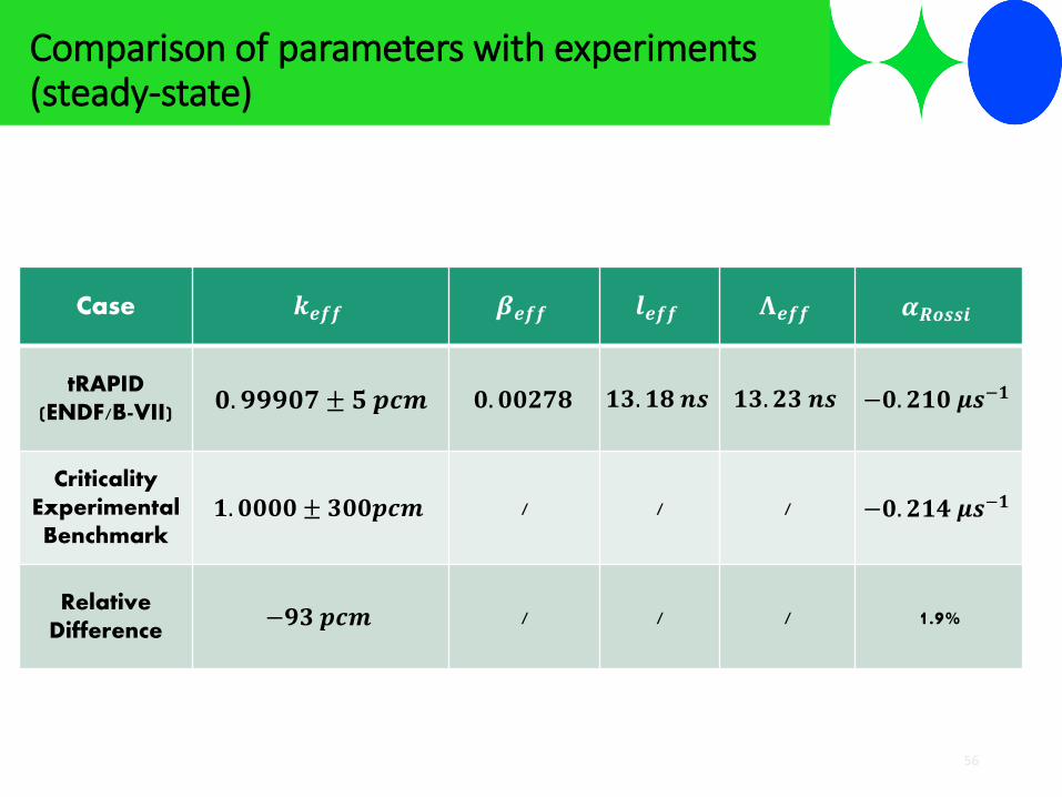
Comparison of parameters with experiments (steady-state)
56
Case 𝒌𝒆𝒇𝒇 𝜷𝒆𝒇𝒇 𝒍𝒆𝒇𝒇 𝚲𝒆𝒇𝒇 𝜶𝑹𝒐𝒔𝒔𝒊
tRAPID(ENDF/B-VII) 𝟎. 𝟗𝟗𝟗𝟎𝟕 ± 𝟓 𝒑𝒄𝒎 𝟎. 𝟎𝟎𝟐𝟕𝟖 𝟏𝟑. 𝟏𝟖 𝒏𝒔 𝟏𝟑. 𝟐𝟑 𝒏𝒔 −𝟎. 𝟐𝟏𝟎 𝝁𝒔−𝟏
Criticality Experimental Benchmark
𝟏. 𝟎𝟎𝟎𝟎 ± 𝟑𝟎𝟎𝒑𝒄𝒎 / / / −𝟎. 𝟐𝟏𝟒 𝝁𝒔−𝟏
Relative Difference
−𝟗𝟑 𝒑𝒄𝒎 / / / 1.9%

Pulsed Neutron the flattop benchmark problem - Serpent vs. tRAPID
57
Computational timeSerpent: 36 min on 32 coresRAPID: 42 s on 1 core

• RAPID is incorporated into a Web application, referred to as the Virtual Reality System (VRS) for RAPID.
• VRS-RAPID provides a collaborative Virtual Reality environment for a user to build models, perform simulation, and view 3-D diagrams in an interactive mode.
• 3-D diagrams can be projected onto a virtual system environment (e.g., a pool) for further analysis and training purposes.
• Additionally, VRS-RAPID outputs can be coupled with an immersive facility such as the VT’s HyberCube System, as shown in this figure.
58
VRS-RAPID* Web Application
*Filed a disclosure application to the VT-IP Office, March 2, 2018
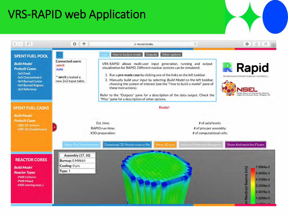
VRS-RAPID web Application
59

• Thus far, RAPID has been used for
• Simulation of spent fuel pools and storage casks, and reactor cores; demonstrated the accuracy of RAPID against MCNP and Serpent codes for variable burnups (axial & radial) for obtained pin-wise, axially-dependent fission density in real time.
• Current capability
• Calculates system eigenvalue, subcritical multiplication, axially-dependent pin-wise fissionneutron, gamma, and/or antineutrino distributions, and detector responses or surface radiation dose.
• When used in conjunction with measurements, e.g., for safeguards application, it can identity potential fuel diversion or misplacement.
• VRS-RAPID provides an excellent environment for analysis and training
• Ongoing work bRAPID: further benchmarking for different applications DRF algorithm: further benchmarking for different applications tRAPID: developing time-dependent algorithms for RAPID for reactor kinetics (solid and
liquid fuel) Patent application (pending) Discussion with interested parties, and exploring marketing and the use of RAPID for real-
world applications and training
60
Status of RAPID

Thanks!
Questions?
61