FINAL REPORT Demonstration of Advanced Geophysics and Classification

Technologies on Munitions Response Sites Pole Mountain Target and Maneuver Area, Wyoming

ESTCP Project MR-201161

March 2012

Victoria Kantsios Brian Helmlinger Darrell Hall Tom King URS Group, Inc.

Standard Form 298 (Rev. 8/98)

REPORT DOCUMENTATION PAGE

Prescribed by ANSI Std. Z39.18

Form Approved OMB No. 0704-0188

The public reporting burden for this collection of information is estimated to average 1 hour per response, including the time for reviewing instructions, searching existing data sources, gathering and maintaining the data needed, and completing and reviewing the collection of information. Send comments regarding this burden estimate or any other aspect of this collection of information, including suggestions for reducing the burden, to the Department of Defense, Executive Services and Communications Directorate (0704-0188). Respondents should be aware that notwithstanding any other provision of law, no person shall be subject to any penalty for failing to comply with a collection of information if it does not display a currently valid OMB control number. PLEASE DO NOT RETURN YOUR FORM TO THE ABOVE ORGANIZATION. 1. REPORT DATE (DD-MM-YYYY) 2. REPORT TYPE 3. DATES COVERED (From - To)

4. TITLE AND SUBTITLE 5a. CONTRACT NUMBER

5b. GRANT NUMBER

5c. PROGRAM ELEMENT NUMBER

5d. PROJECT NUMBER

5e. TASK NUMBER

5f. WORK UNIT NUMBER

6. AUTHOR(S)

7. PERFORMING ORGANIZATION NAME(S) AND ADDRESS(ES) 8. PERFORMING ORGANIZATION REPORT NUMBER

9. SPONSORING/MONITORING AGENCY NAME(S) AND ADDRESS(ES) 10. SPONSOR/MONITOR'S ACRONYM(S)

11. SPONSOR/MONITOR'S REPORT NUMBER(S)

12. DISTRIBUTION/AVAILABILITY STATEMENT

13. SUPPLEMENTARY NOTES

14. ABSTRACT

15. SUBJECT TERMS

16. SECURITY CLASSIFICATION OF: a. REPORT b. ABSTRACT c. THIS PAGE

17. LIMITATION OF ABSTRACT

18. NUMBER OF PAGES

19a. NAME OF RESPONSIBLE PERSON

19b. TELEPHONE NUMBER (Include area code)

27-03-2012 Final Report May 2011 - March 2012

Demonstration of Advanced Geophysics and Classification Technologies on Munitions Response Sites Pole Mountain Target and Maneuver Area, Wyoming

W912HQ-11-C-0024

MR-201161V. Kantsios, B. Helmlinger, D. Hall, T. King

URS Group, Incorporated 2450 Crystal Drive, Suite 500 Arlington, VA 22202

Environmental Security Technology Certification Program (ESTCP) Office 901 North Stuart Street, Suite 303 Arlington, VA 22203

ESTCP

Approved for public release; distribution is unlimited.

This document serves as the Environmental Security Technology Certification Program (ESTCP) Demonstration Report for the Demonstration of Advanced Geophysics and Classification Technologies on the Bisbee Hill Maneuver Area Munitions Response Site (MRS). This MRS is located within the former Pole Mountain Target and Maneuver Area (PMTMA) Munitions Response Area, located in the Medicine Bowl National Forest, Wyoming. This project is one in a series of projects funded by ESTCP to test the effectiveness of advanced geophysical sensors and physics-based data analysis tools for anomaly classification.

Unclassified Unclassified Unclassified UL 68

V. Kantsios

(703) 418-3030

Reset

iii

TABLE OF CONTENTS

1.0  INTRODUCTION .............................................................................................................. 1 1.1  BACKGROUND .................................................................................................... 1 1.2  OBJECTIVE OF THE DEMONSTRATION ......................................................... 1 1.3  REGULATORY DRIVER...................................................................................... 1 

2.0  TECHNOLOGY ................................................................................................................. 2 2.1  TECHNOLOGY DESCRIPTION .......................................................................... 2 

2.1.1  Digital Geophysical Mapping ..................................................................... 2 2.1.2  Anomaly Classification Methods ................................................................ 2 

2.2  TECHNOLOGY DEVELOPMENT ....................................................................... 3 2.3  ADVANTAGES AND LIMITATIONS OF THE TECHNOLOGY ...................... 3 

3.0  PERFORMANCE OBJECTIVES ...................................................................................... 5 3.1  OBJECTIVE: ALONG-LINE MEASUREMENT SPACING ............................... 6 3.2  OBJECTIVE: COMPLETE COVERAGE OF THE DEMONSTRATION SITE . 6 3.3  OBJECTIVE: DETECTION OF ALL TARGETS OF INTEREST ....................... 6 3.4  OBJECTIVE: MAXIMIZE CORRECT CLASSIFICATION OF TARGETS

OF INTEREST........................................................................................................ 7 3.5  OBJECTIVE: MAXIMIZE CORRECT CLASSIFICATION OF NON-

TARGETS OF INTEREST..................................................................................... 7 3.6  OBJECTIVE: SPECIFICATION OF NO-DIG THRESHOLD ............................. 7 3.7  OBJECTIVE: MINIMIZE NUMBER OF ANOMALIES THAT CANNOT BE

ANALYZED ........................................................................................................... 7 3.8  OBJECTIVE: CATEGORY 0 TARGETS CLASSIFIED CORRECTLY ............. 8 3.9  OBJECTIVE: CORRECTLY EXTRACT FEATURE SCALARS ........................ 8 3.10  OBJECTIVE: CORRECTLY CLASSIFY CATEGORY 2 TARGETS ................. 8 

4.0  SITE DESCRIPTION ......................................................................................................... 9 4.1  SITE SELECTION ................................................................................................. 9 4.2  SITE HISTORY ...................................................................................................... 9 4.3  SITE GEOLOGY .................................................................................................... 9 4.4  MUNITIONS CONTAMINATION ..................................................................... 11 

5.0  TEST DESIGN ................................................................................................................. 12 5.1  CONCEPTUAL EXPERIMENTAL DESIGN ..................................................... 12 5.2  SITE PREPARATION.......................................................................................... 12 5.3  CALIBRATION ACTIVITIES – INSTRUMENT VERIFICATION STRIP ...... 13 5.4  DATA COLLECTION – EM61-MK2 GEOPHYSICAL SURVEY .................... 13 

5.4.1  Scale .......................................................................................................... 13 5.4.2  Sample Density ......................................................................................... 15 5.4.3  Quality Checks .......................................................................................... 15 5.4.4  Data Summary .......................................................................................... 16 

5.5  VALIDATION ...................................................................................................... 18 5.5.1  Excavation Procedure ............................................................................... 18 5.5.2  Data Recording Procedure ........................................................................ 19 5.5.3  Post Clearance ........................................................................................... 19 

iv

5.5.4  Validation Results ..................................................................................... 19 

6.0  DATA ANALYSIS AND PRODUCTS ........................................................................... 20 6.1  EM61-MK2 DGM DATA PROCESSING AND INTERPRETATION .............. 20 

6.1.1  Processing ................................................................................................. 20 6.1.2  Target Selection for Detection .................................................................. 21 

6.2  METAL MAPPER CUED DATA ANALYSIS AND CLASSIFICATION METHODS ........................................................................................................... 21 6.2.1  Overview of the Classification Process .................................................... 21 6.2.2  Target Parameterization ............................................................................ 24 6.2.3  Rule-Based Decisions ............................................................................... 25 6.2.4  Classifiers (Target of Interest Indicator Tools) ......................................... 33 6.2.5  Data Products ............................................................................................ 37 

7.0  PERFORMANCE ASSESSMENT .................................................................................. 42 7.1  OBJECTIVE: ALONG-LINE MEASUREMENT SPACING ............................. 43 

7.1.1  Metric ........................................................................................................ 43 7.1.2  Data Requirements .................................................................................... 43 7.1.3  Success Criteria ......................................................................................... 43 7.1.4  Results ....................................................................................................... 43 

7.2  OBJECTIVE: COMPLETE COVERAGE OF THE DEMONSTRATION SITE 44 7.2.1  Metric ........................................................................................................ 44 7.2.2  Data Requirements .................................................................................... 44 7.2.3  Success Criteria ......................................................................................... 44 7.2.4  Results ....................................................................................................... 44 

7.3  OBJECTIVE: DETECTION OF ALL TARGETS OF INTEREST ..................... 46 7.3.1  Metric ........................................................................................................ 46 7.3.2  Data Requirements .................................................................................... 46 7.3.3  Success Criteria ......................................................................................... 46 7.3.4  Results ....................................................................................................... 47 

7.4  OBJECTIVE: MAXIMIZE CORRECT CLASSIFICATION OF TARGETS OF INTEREST...................................................................................................... 47 7.4.1  Metric ........................................................................................................ 47 7.4.2  Data Requirements .................................................................................... 47 7.4.3  Success Criteria ......................................................................................... 48 7.4.4  Results ....................................................................................................... 48 

7.5  OBJECTIVE: MAXIMIZE CORRECT CLASSIFICATION OF NON-TARGETS OF INTEREST................................................................................... 48 7.5.1  Metric ........................................................................................................ 48 7.5.2  Data Requirements .................................................................................... 48 7.5.3  Success Criteria ......................................................................................... 48 7.5.4  Results ....................................................................................................... 48 

7.6  OBJECTIVE: SPECIFICATION OF NO-DIG THRESHOLD ........................... 48 7.6.1  Metric ........................................................................................................ 49 7.6.2  Data Requirements .................................................................................... 49 7.6.3  Success Criteria ......................................................................................... 49 7.6.4  Results ....................................................................................................... 49 

v

7.7  OBJECTIVE: MINIMIZE NUMBER OF ANOMALIES THAT CANNOT BE ANALYZED ......................................................................................................... 49 7.7.1  Metric ........................................................................................................ 49 7.7.2  Data Requirements .................................................................................... 49 7.7.3  Success Criteria ......................................................................................... 49 7.7.4  Results ....................................................................................................... 49 

7.8  OBJECTIVE: CORRECTLY CLASSIFY CATEGORY 0 TARGETS ............... 50 7.8.1  Metric ........................................................................................................ 50 7.8.2  Data Requirements .................................................................................... 50 7.8.3  Success Criteria ......................................................................................... 50 7.8.4  Results ....................................................................................................... 50 

7.9  OBJECTIVE: CORRECTLY EXTRACT FEATURE SCALARS ...................... 50 7.9.1  Metric ........................................................................................................ 51 7.9.2  Data Requirements .................................................................................... 51 7.9.3  Success Criteria ......................................................................................... 51 7.9.4  Results ....................................................................................................... 51 

7.10  OBJECTIVE: CORRECTLY CLASSIFY CATEGORY 2 TARGETS ............... 51 7.10.1  Metric ........................................................................................................ 51 7.10.2  Data Requirements .................................................................................... 51 7.10.3  Success Criteria ......................................................................................... 51 7.10.4  Results ....................................................................................................... 51 

8.0  COST ASSESSMENT ...................................................................................................... 52 

9.0  IMPLEMENTATION ISSUES ........................................................................................ 53 

10.0  REFERENCES ................................................................................................................. 55  Appendix A: POINTS OF CONTACT

vi

FIGURES Figure 1. ESTCP PMTMA Demonstration Area Map.................................................................. 10 Figure 2. Geophysical Grid Locations .......................................................................................... 14 Figure 3. IVS LFO/MFO Plot for Team 2 for the 75mm Projectile Seed Item ............................ 17 Figure 4. IVS Positioning Plot for Team 2 for the 75mm Projectile Seed Item ........................... 18 Figure 5. PMTMA EM61-MK2 Production Data Channel 2 Survey Results .............................. 22 Figure 6. PMTMA EM61-MK2 Production Data with 2,370 Selected Targets and Grid Frame . 23 Figure 7. Simplified Block Diagram Illustrating the Processing Steps Used to Generate a

Prioritized Dig List ................................................................................................................... 24 Figure 8. PMTMA Cued Production Data Signal Amplitude Statistics ....................................... 26 Figure 9. PMTMA Cued Production Data Fit Statistics (Cohesion and Correlation

Coefficient) .............................................................................................................................. 27 Figure 10. PMTMA Cued Production Data Displacement Statistics (Horizontal Offset and

Depth) ....................................................................................................................................... 27 Figure 11. PMTMA Cued Production Data P0x Statistics (Target Size) ....................................... 27 Figure 12. Data Confidence Penalty Sub-Functions f and g ......................................................... 30 Figure 13. Distribution of Possible Ordnance (Interpretation From Polarizability Curves) and

IVS/Test Pit Data for PMTMA Data ....................................................................................... 32 Figure 14. Distribution of PMTMA Data (Possible Ordnance Based on Interpretation From

Polarizability Curves) .............................................................................................................. 32 Figure 15. Five Best Trained ANN ROC Results ......................................................................... 35 Figure 16. DLRT Output Results Scatter Plot, P0x vs τ0x ............................................................. 36 Figure 17. LM of Historic Ordnance Documented at PMTMA ................................................... 38 Figure 18. ANN, LM, and Short Category 0 List ......................................................................... 39 Figure 19. ANN, DLRT Short, LM, and Short Category 0 List ................................................... 40 Figure 20. ANN, DLRT Long, LM, and Short Category 0 List ................................................... 40 Figure 21. ANN, DLRT Long, LM, and Long Category 0 List ................................................... 41 Figure 22. PMTMA Footprint Coverage Plot Using a Width of 0.5 m ........................................ 45 Figure 23. PMTMA Footprint Coverage Plot Using a Width of 0.75 m ...................................... 46 Figure 24. PMTMA EM61-MK2 Production Data With All 160 QC Seed Items Identified ....... 47 Figure 25. Footprints of targets 2154 and 2330 (37mm) and targets 2132 and 2057 (ISOs) ....... 50 

vii

TABLES Table 1. Quantitative Performance Objectives for this Demonstration .......................................... 5 Table 2. PMTMA Instrument Verification Strip .......................................................................... 13 Table 3. Multi-Line Response of Some Small Items .................................................................... 29 Table 4. Target of Interest Size Statistics ..................................................................................... 31 Table 5. Five Best Trained ANN Results ..................................................................................... 34 Table 6. DLRT Nearest Neighbor Identified TOI ........................................................................ 36 Table 7. General Target List Statistics .......................................................................................... 39 Table 8. Quantitative Performance Objectives for This Demonstration ....................................... 42 Table 9. Minimization of Non-TOI Results .................................................................................. 48 Table 10. Project Costs ................................................................................................................. 52 

viii

ACRONYMS ANN Artificial Neural Network ASCII American Standard Code for Information Interchange CERCLA Comprehensive Environmental Response, Compensation, and Liability Act DERP Defense Environmental Restoration Program DGM Digital Geophysical Mapping DLRT Distance Likelihood Ratio Tests DoD Department of Defense DQO Data Quality Objective EMI Electromagnetic Induction ESTCP Environmental Security Technology Certification Program GPS Global Positioning System GSV Geophysical System Verification HE High Explosive ISO Industry Standard Object IVS Instrument Verification Strip LFO/MFO Least Favorable Orientation/Most Favorable Orientation LM Library Matching MEC Munitions and Explosives of Concern MLP Multi-layer Perceptron MM MetalMapper MMRP Military Munitions Response Program MPPEH Material Potentially Presenting an Explosive Hazard MRS Munitions Response Site µs Microseconds mV Millivolts NCP National Oil and Hazardous Substances Pollution Contingency Plan PMTMA Pole Mountain Training and Maneuver Area QAPP Quality Assurance Project Plan QC Quality Control RBA Rule-Based Analysis ROC Receiver Operating Characteristic RTK Real Time Kinematic SARA Superfund Amendments and Reauthorization Act SERDP Strategic Environmental Research and Development Program SLO San Luis Obispo SNR Signal-to-Noise Ratio TOI Target of Interest URS URS Group, Inc. USACE U.S. Army Corps of Engineers UTM Universal Transverse Mercator UXO Unexploded Ordnance

1

1.0 INTRODUCTION

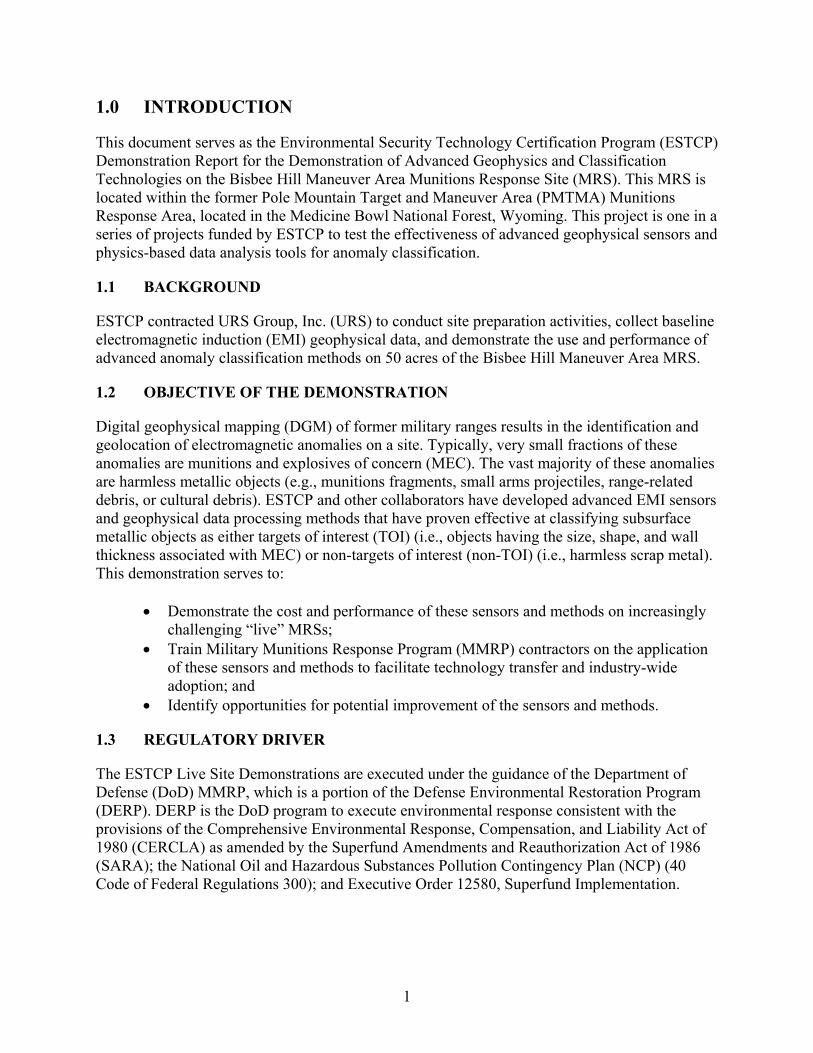
This document serves as the Environmental Security Technology Certification Program (ESTCP) Demonstration Report for the Demonstration of Advanced Geophysics and Classification Technologies on the Bisbee Hill Maneuver Area Munitions Response Site (MRS). This MRS is located within the former Pole Mountain Target and Maneuver Area (PMTMA) Munitions Response Area, located in the Medicine Bowl National Forest, Wyoming. This project is one in a series of projects funded by ESTCP to test the effectiveness of advanced geophysical sensors and physics-based data analysis tools for anomaly classification.

1.1 BACKGROUND

ESTCP contracted URS Group, Inc. (URS) to conduct site preparation activities, collect baseline electromagnetic induction (EMI) geophysical data, and demonstrate the use and performance of advanced anomaly classification methods on 50 acres of the Bisbee Hill Maneuver Area MRS.

1.2 OBJECTIVE OF THE DEMONSTRATION

Digital geophysical mapping (DGM) of former military ranges results in the identification and geolocation of electromagnetic anomalies on a site. Typically, very small fractions of these anomalies are munitions and explosives of concern (MEC). The vast majority of these anomalies are harmless metallic objects (e.g., munitions fragments, small arms projectiles, range-related debris, or cultural debris). ESTCP and other collaborators have developed advanced EMI sensors and geophysical data processing methods that have proven effective at classifying subsurface metallic objects as either targets of interest (TOI) (i.e., objects having the size, shape, and wall thickness associated with MEC) or non-targets of interest (non-TOI) (i.e., harmless scrap metal). This demonstration serves to:

Demonstrate the cost and performance of these sensors and methods on increasingly challenging “live” MRSs;

Train Military Munitions Response Program (MMRP) contractors on the application of these sensors and methods to facilitate technology transfer and industry-wide adoption; and

Identify opportunities for potential improvement of the sensors and methods.

1.3 REGULATORY DRIVER

The ESTCP Live Site Demonstrations are executed under the guidance of the Department of Defense (DoD) MMRP, which is a portion of the Defense Environmental Restoration Program (DERP). DERP is the DoD program to execute environmental response consistent with the provisions of the Comprehensive Environmental Response, Compensation, and Liability Act of 1980 (CERCLA) as amended by the Superfund Amendments and Reauthorization Act of 1986 (SARA); the National Oil and Hazardous Substances Pollution Contingency Plan (NCP) (40 Code of Federal Regulations 300); and Executive Order 12580, Superfund Implementation.

2

2.0 TECHNOLOGY

A Geonics EM61-MK2, paired with a Trimble R8 Real Time Kinetic (RTK) Global Positioning System (GPS), was used to conduct the DGM survey over the demonstration site. Anomalies were identified and subsequently analyzed using a Geometrics MetalMapper (MM) under a separate contract by a private contractor. The MM output, advanced cued geophysical data, were analyzed to classify anomalies as TOI or non-TOI using a combination of tools, including rule-based analysis (RBA), artificial neural networks (ANN), distance likelihood ratio testing (DLRT), and library matching (LM). URS used several software applications, including Geosoft’s Oasis Montaj UX-Analyze extension, Statistica (statistical analysis tools), MATLAB, Mathematica, and C++ software developed by URS.

2.1 TECHNOLOGY DESCRIPTION

2.1.1 Digital Geophysical Mapping

The baseline DGM survey was performed using a Geonics EM61-MK2, paired with a Trimble R8 RTK GPS, and an Allegro CX field computer. The EM61-MK2 system consisted of a 1.0 m by 0.5 m coil containing both a transmitter and receiver antenna. The lower coil was located 42 cm above the ground surface for optimal data collection using the standard wheel mode. Cross-line spacing during the survey was maintained using rope stretched between two measuring tapes. DGM data were corrected and processed using NAV61 and DAT61 software to convert binary files in American Standard Code for Information Interchange (ASCII) format and to interpolate locations for each DGM sample. Oasis Montaj was then used to:

Convert location data from latitude and longitude to Universal Transverse Mercator (UTM) Zone 13 North, Meters;

Identify and apply latency corrections;

Level data to remove instrument drift using an iterative filter that subtracted median values of background noise from the data;

Grid data using a minimum curvature algorithm;

Test cross-line and down-line spacing to ensure compliance with project metrics; and

Identify target responses above the threshold using the Blakley method. URS selected anomalies for advanced classification using a target response-based procedure. The threshold for target anomaly selection was set at 5.2 mV in channel 2 (i.e., the cart-mounted EM61-MK2 response expected from a horizontal 37mm projectile at a depth of 30 cm).

2.1.2 Anomaly Classification Methods

URS applied an innovative hybrid classification methodology to classify anomalies as TOI and non-TOI. Cued anomaly data were collected by a private contractor using MM and provided to URS by the ESTCP Program Office. URS utilized previous experience processing and analyzing

3

similar data and built upon traditional techniques using Geosoft’s Oasis Montaj UX-Analyze software package utilities as well as new classification processes. Anomalies were classified into four categories:

Category 0: Cannot analyze

Category 1: Likely TOI

Category 2: Cannot decide

Category 3: Likely non-TOI URS employed Geosoft’s Oasis Montaj UX-Analyze inversion routines for single and multi-source results to extract the principal polarizability transient curves from the cued MM data. Then feature vectors were derived from transient curves using C++ algorithms. The URS classification scheme applied RBA to determine the Category 0 and 3 targets. Thereafter, ANN and/or DLRT were used to classify the targets. Finally, LM was applied to move poorly classified targets from Categories 2 and 3 into Category 1. Details of the classification methodology are described in Section 6.

2.2 TECHNOLOGY DEVELOPMENT

The use of ANN to discriminate between TOI and non-TOI has been established by previous investigators (Geometrics 2010; Szidarovsky, Poulton, and MacInnes 2008). However, ANN results are often strongly polarized with scalar values either very close to 1 or 0 and few around 0.5, the ambiguous zone. In previous classification studies, the resolution has been to allow LM to change these “bad” ANN classifications from non-TOI to TOI. To reduce reliance on LM, a nearest neighbor type classifier was investigated with the idea that the ANN output temporarily identified as non-TOI could be re-ordered by the nearest neighbor type classifier. By this re-ordering, targets near to ANN-identified TOI in feature space could also be identified as TOI. DLRT was chosen due to its strong performance with respect to other nearest neighbor classifier algorithms (Remus 2011; Remus et al. 2008).

2.3 ADVANTAGES AND LIMITATIONS OF THE TECHNOLOGY

Hybrid classifiers provide a more robust means of classification than a single classifier tool. ANN based approaches have been successfully paired with LM in previous demonstrations, where ANN has reduced the number of TOI over LM alone, and LM has reduced the number of false negatives resulting from ANN alone. DLRT offers an additional “fail safe” by prioritizing those targets closest to ANN-identified TOI. The disadvantage of a hybrid classifier is that the number of potential TOI that are to be dug is usually increased. DLRT is a nearest neighbor technique that is applied using the ANN TOI results as inputs into DLRT. Therefore, ANN TOI located near the ANN decision surface often influence DLRT to select targets outside the ANN decision surface, increasing the number of TOI. DLRT used in this manner often contradicts the ANN results by increasing the number of

4

TOI. This trade-off is acceptable since the new hybrid system allows much greater control of the location of the decision surface of the final classifier.

5

3.0 PERFORMANCE OBJECTIVES

Performance objectives for the demonstration, provided in Table 1, serve as a basis for the evaluation of the performance and costs of the demonstrated technology. These objectives are for the baseline EM61-MK2 data collection and the MM data analysis and classification.

Table 1. Quantitative Performance Objectives for this Demonstration Performance

Objective Metric Data Required Success Criteria Results

EM61-MK2 Data Collection Objectives

Along-line measurement spacing

Point-to-point spacing from data set

Mapped production survey data

90% <15 cm along-line spacing

Data quality objective (DQO) achieved with exception noted in Section 7.1.4

Complete coverage of the demonstration site

Footprint coverage Mapped production survey data

≥85% coverage at 0.5 m line spacing and ≥98% coverage at 0.75 m line spacing calculated using UX-Process Footprint Coverage QC Tool

DQO achieved

Detection of all TOI Percent detected of seeded items

Location of seeded items and anomaly list

100% of seeded items detected

DQO achieved

MM Data Analysis and Classification Objectives

Maximize correct classification of TOI

Percent of TOI placed in Category 1

Prioritized anomaly lists and dig results

Correctly classify 100% of TOI

DQO achieved

Maximize correct classification of non-TOI

Percent of correctly classified non-TOI

Prioritized anomaly lists and dig results

>65% of non-TOI classified in Category 3

DQO achieved

Specification of no-dig threshold

Percent of TOI placed in Categories 1 or 2 and percent of non-TOI placed in Category 3.

MM cued data, prioritized anomaly lists, and dig results

100% of TOI placed in Categories 1 and 2. >65% of non-TOI placed in Category 3.

DQO achieved

Minimize number of anomalies that cannot be analyzed

Percentage of anomalies classified as Category 0

Inverted MM cued data and prioritized anomaly dig list

Reliable target parameters can be estimated for >95% of anomalies on each sensor’s detection list

DQO achieved

Category 0 targets are categorized correctly

The polarization curves visually reflect a non-analyzable target

Inverted MM cued data and polarization curves

All targets placed in the “Can’t Analyze” category will have polarization curves reflecting a non-analyzable target.

DQO achieved

Correctly extract feature scalars

Category 1 TOI should cluster in various feature space scatter plots

Derived target feature vectors, inverted MM cued data, and polarization curves

Various feature space scatter plots display distinct clustering

DQO achieved

6

Performance Objective

Metric Data Required Success Criteria Results

Correctly classify Category 2 targets

Category 2 targets should display TOI-like properties

Polarization curves, derived target feature vectors, and dig results

Category 2 targets should be proximal to TOI clusters and/or polarization curves display TOI characteristics

DQO achieved

3.1 OBJECTIVE: ALONG-LINE MEASUREMENT SPACING

Description: Down-line data must be sufficiently dense to support detection of all anomalies and minimal data gaps.

Metric: Along track point-to-point data spacing measured using EM61-MK2 and RTK GPS point positioning.

Data Requirements: Mapped production survey data.

Success Criteria: Ninety percent of the production data will have a point-to-point displacement of <15 cm.

3.2 OBJECTIVE: COMPLETE COVERAGE OF THE DEMONSTRATION SITE

Description: The EM61-MK2 baseline data were used to identify metallic anomalies on the demonstration site for further analysis. Therefore, the expectation is complete mapping of the accessible areas of the site.

Metric: Complete coverage of the demonstration site.

Data Requirements: Mapped production survey data used to generate grids to allow for target picking.

Success Criteria: Greater than 85% coverage at 0.5 m line spacing and greater than 98% coverage at 0.75 m line spacing calculated using UX-Process Footprint Coverage QC Tool.

3.3 OBJECTIVE: DETECTION OF ALL TARGETS OF INTEREST

Description: Quality EM61-MK2 data should lead to a high probability of detecting TOI on the site.

Metric: Detect the seed items using the specified anomaly selection threshold of 5.2 mV in channel 2.

Data Requirements: The anomaly list (and locations) selected by the processing geophysicist, and the list and location of seed items visible only to the quality control (QC) geophysicist.

Success Criteria: 100% of the seeded items detected.

7

3.4 OBJECTIVE: MAXIMIZE CORRECT CLASSIFICATION OF TARGETS OF INTEREST

Description: Correctly classify TOI.

Metric: Percentage of TOI correctly classified as Category 1 using each classification approach.

Data Requirements: Prioritized dig list for each classification approach using provided target list in conjunction with a classification strategy. Results of validation digging.

Success Criteria: Each of the classification approaches correctly identifies all TOI in Category 1.

3.5 OBJECTIVE: MAXIMIZE CORRECT CLASSIFICATION OF NON-TARGETS OF INTEREST

Description: Correctly classify non-TOI.

Metric: Percentage of correctly classified non-TOI using each classification approach.

Data Requirements: Prioritized dig list for each classification approach using provided target list in conjunction with a classification strategy. Results of validation digging.

Success Criteria: >65% of non-TOI are classified in Category 3.

3.6 OBJECTIVE: SPECIFICATION OF NO-DIG THRESHOLD

Description: Correctly establish the dig/no-dig threshold.

Metric: Percent of TOI placed in Categories 1 or 2 and percent of non-TOI placed in Category 3.

Data Requirements: MetalMapper cued data, prioritized anomaly lists, and validation digging results.

Success Criteria: 100% of TOI are identified in Category 1 or 2 and >65% of non-TOI are identified in Category 3.

3.7 OBJECTIVE: MINIMIZE NUMBER OF ANOMALIES THAT CANNOT BE ANALYZED

Description: Minimize the number of anomalies that cannot be analyzed.

Metric: The percentage of anomalies classified as Category 0.

Data Requirements: Inverted MM cued data and prioritized anomaly lists.

Success Criteria: Less than 5% of the data in Category 0.

8

3.8 OBJECTIVE: CATEGORY 0 TARGETS CLASSIFIED CORRECTLY

Description: Verify that Category 0 targets are correctly classified.

Metric: Percent of polarization curves in Category 0 that visually reflect a non-analyzable target.

Data Requirements: Inverted MM cued data and polarization curves.

Success Criteria: All targets placed in Category 0 will have polarization curves reflecting a non-analyzable target.

3.9 OBJECTIVE: CORRECTLY EXTRACT FEATURE SCALARS

Description: Extract the feature scalars for the MM cued inversion results.

Metric: Degree of clustering displayed in feature space scatter plots for various TOIs.

Data Requirements: Inverted MM cued inversion results, polarization curves, and derived features scalars.

Success Criteria: Various feature space scatter plots for TOI display distinct clustering.

3.10 OBJECTIVE: CORRECTLY CLASSIFY CATEGORY 2 TARGETS

Description: Verify that Category 2 targets are correctly classified.

Metric: Category 2 feature scalars should visually plot closely to Category 1 targets.

Data Requirements: Derived feature scalars, polarization curves, and validation digging results.

Success Criteria: Category 2 targets should be proximal to TOI clusters and/or polarization curves display TOI characteristics.

9

4.0 SITE DESCRIPTION

The 50-acre demonstration area is located within the Bisbee Hill Maneuver Area MRS, located in the north-central portion of PMTMA (see Figure 1).

4.1 SITE SELECTION

ESTCP selected this MRS because of its wide mixture of munitions and variable terrain. The smallest known munitions type on the site is the 37mm projectile; the largest known are 3-in. projectiles and mortars, with a range of munitions sizes in between.

4.2 SITE HISTORY

This site was used for military maneuvers and contained the primary bivouac site for the PMTMA facility. An artillery impact area was located between two observation bunkers at Bisbee Hill and Merritt Hill. The two bunkers were constructed in 1941 to observe artillery practice of the 183rd and 188th Field Artillery Regiments of the National Guard. Additional military features identified in the MRS include small bunkers and trenches. Due to the varied multi-use nature of PMTMA, other range operations may have occurred within this MRS. During the Engineering Evaluation/Cost Analysis, a 75mm projectile with high explosive (HE) filler was found at the ground surface approximately 750 ft east of Happy Jack Road (Highway 210), midway between Bisbee Hill and Forest Service Road 732 (Earth Tech 2000). The Archive Search Report team also reported blank small arms ammunition, but small arms ammunition poses no significant explosive hazard. Historical and physical evidence indicate that MEC within the Bisbee Hill Maneuver Area MRS could include 75mm projectiles [U.S. Army Corps of Engineers (USACE) 1996].

4.3 SITE GEOLOGY

Cretaceous-age rocks underlying the area include the Fox Hills Sandstone and the Laramie Formation. Tertiary-age rocks are composed of the Chadron Formation, the Brule Formation, the Arikaree Formation, and the Ogallala Formation. Outcrops of the Chadron Formation in the vicinity of Pole Mountain consist mainly of medium- to coarse-grained brown sandstone. The Brule Formation is a hard, compact, brittle bentonitic siltstone that is locally sandy or argillaceous. The Arikaree Formation consists mainly of massive to poorly bedded, fine- to medium-grained, loose- to moderately-cemented, gray to brown sand containing lenses of pipy concretions of very hard, tough, brownish-gray to dark gray sandstone that is cemented with calcium carbonate. The Ogallala Formation consists of lenticular deposits of heterogeneous materials and is the surface formation of the upland area lying east of the Laramie Range and north of the Wyoming-Colorado state line (USACE 1996). Surface soil throughout Pole Mountain is relatively shallow (<20 in. deep) and is predominantly rocky with rock outcrop components.

10

Figure 1. ESTCP PMTMA Demonstration Area Map

'----

LEGEND CJ Munitions Response Area

~ : :• Pole Mountain FUDS Boundary

c::::J Munitions Response Site (MRS)

CJ ESTCP Demonstration Site

N

NAD _1983_ UTM_Zone_13N 0 05 1

~

Bisbee Hlll~neuver Area

2 I Miles

FIGURE NUMBER

1·1

U.S. ARMY CORPS OF ENGINEERS

OMAHA DISTRICT

MI~ITARY MUNITIONS RESPONSE PROGRAM

Munit ions Response Area Po le Mountain Target and

Maneuver Area

11

4.4 MUNITIONS CONTAMINATION

The following MEC hazards were encountered and documented during the previous Remedial Investigation (Innovative Technical Solutions, Inc. 2010):

Projectiles containing HE filler (37mm to 155mm and 2.95 in.);

Shrapnel projectiles (75mm and 3 in.);

37mm projectiles (inert and unfuzed)

3-in. Stokes mortars (practice, fuzed);

60mm mortars containing HE filler; and

Small arms ammunition (.30 caliber and .50 caliber).

12

5.0 TEST DESIGN

URS had two roles in this project:

Overall site management (e.g., site preparation, DGM, and validation digging) and Advanced instrument data analysis and anomaly classification.

During site preparation activities, URS seeded the demonstration area and collected baseline geophysical mapping with an EM61-MK2. URS geophysicists classified anomalies using MM data collected by a private contractor and provided to URS by the ESTCP Program Office. This section discusses the activities that were executed by URS in support of this project.

5.1 CONCEPTUAL EXPERIMENTAL DESIGN

Demonstration/Work Plan Development: URS prepared a site-specific MEC-Quality Assurance Project Plan (QAPP) in lieu of a traditional work plan for the PMTMA demonstration project (ESTCP 2011).

Site Preparation: URS emplaced 200 seed items in the 50-acre demonstration site that had been previously surface cleared.

Geophysical Data Collection: URS surveyed approximately 50 acres using a cart mounted EM-61 with a line spacing of 0.5 m. Data were processed, targets selected, and data submitted to the ESTCP Program Office.

MM Data Analysis and Classification: URS analyzed 2,370 static MM points for classification. URS geophysicists used a variety of methods to conduct the classification and to produce a dig/no dig list.

Intrusive Investigation: URS intrusively investigated 2,370 anomalies identified by the ESTCP Program Office. Each anomaly was photographed and attribute information (e.g., nomenclature, size, depth, position, and orientation) captured and provided to the ESTCP Program Office.

5.2 SITE PREPARATION

URS seeded the site and established an instrument verification strip (IVS) near the demonstration area. Unexploded ordnance (UXO) Technicians emplaced 160 targets within the demonstration area as follows:

43 inert 37mm projectiles,

10 inert 57mm projectiles,

25 inert 75mm projectiles,

41 inert 60mm mortars,

1 inert 3-in. Stokes mortar, and

40 small industry standard objects (ISOs) (1-in. nominal pipe nipples, 4-in. long).

13

The emplacement team avoided placing seeds in the immediate vicinity of any existing strong anomalies. The ESTCP PMTMA MEC QAPP, Worksheet #17, provides a detailed description of the site preparation and seed emplacement locations and procedures.

5.3 CALIBRATION ACTIVITIES – INSTRUMENT VERIFICATION STRIP

The Project Geophysicist worked in conjunction with UXO Technicians to identify an IVS location based on an initial inspection of the site (including previous geophysical survey data). The final IVS site was free of discrete geophysical anomalies for both the seeded target and background noise lane. URS surveyed the corners of the IVS and the location of each emplaced seed item using RTK GPS. The IVS contained five seed items of the size, location, depth, and orientations listed in Table 2. All seed items were placed horizontally, without inclination/declination.

Table 2. PMTMA Instrument Verification Strip Item ID Description Easting (m) Northing (m) Depth (m) Inclination Orientation

T-001 Shotput 468927.14 4566543.68 0.3 NA NA T-002 Small ISO 468921.99 4566543.61 0.15 Horizontal Across Track T-003 Small ISO 468917.32 4566543.46 0.15 Horizontal Along Track T-004 37mm projectile 468912.22 4566543.40 0.15 Horizontal Across Track T-005 75mm projectile 468907.28 4566543.33 0.15 Horizontal Across Track

URS surveyed the IVS twice daily to verify the proper operation and functioning of the production geophysical equipment and to measure site background noise values for each EM61 system before and after each day of field data collection. The IVS was installed and operated consistently with the specifications and descriptions contained in Geophysical System Verification (GSV): A Physics-Based Alternative to Geophysical Prove Outs for Munitions Response (ESTCP 2009). Standard reference items seeded in the IVS were observed in the data with signals consistent with both historical measurements and physics-based model predictions. The IVS also served to verify the RTK GPS provided accurate sensor location data. ISOs and inert munitions were used as reference seed items. ISOs are commonly available Schedule 40, 1 in. by 4 in. pipe nipples, threaded on both ends, made from black welded steel. EM61-MK2 standard response curves and polar displacement plots for the seeded items are located in Appendix B.

5.4 DATA COLLECTION – EM61-MK2 GEOPHYSICAL SURVEY

5.4.1 Scale

URS conducted a 100% coverage geophysical survey to identify and locate all anomalies within the 50-acre demonstration site using EM61-MK2 all-metals detectors coupled with RTK GPS locating systems. Prior to data collection, the entire site was surveyed into 30-m by 60-m sub-areas or grids, with grid corners marked by numbered lathe. The grid layout and naming convention are shown in Figure 2.

14

Figure 2. Geophysical Grid Locations

15

5.4.2 Sample Density

All data were collected at a sample frequency of 10 Hz. Sample density, including cross-line and along-line spacing, results are discussed in Section 7.1 and Section 7.2. For each grid the team laid out survey tape on each of the longer, 60 m sides of the grid. Two strands of twine separated by 0.5 m were then laid across the shorter side of the grid typically from the southwest to southeast corners. The instrument operator performed the survey by walking directly down the twine in alternating passes. After two alternating passes, the twine was picked up by the other team members and moved 1 m down the survey tape. This procedure was repeated until the entire grid was surveyed by sequential, alternating passes, and allowed for strict control of the spacing between alternating transects. To allow direct comparison between survey files, the survey tape and twine were laid out so that data collection was started and finished with at least one pass inside the adjacent grids on either side of the surveyed grid. After completion of each grid, the field team continued to record data while traversing through the grid and circling each obstacle within the grid (rocks, trees, large shrubs, etc.) that might have resulted in a gap in coverage. To fill gaps identified by the data processor, the field teams returned to the grid where the gap was identified and collected data on a series of transects identified by the data processor. These “gap fill” transects always included significant overlap of adjacent data to allow comparison between datasets and to ensure that each gap was completely filled.

5.4.3 Quality Checks

Daily field activities were coordinated during the morning briefing to ensure that the field teams maintained sufficient separation throughout the day to prevent interference between EM61 sensors. After completing the tailgate safety brief, the field teams performed a minimum 15-minute instrument warm-up to allow the EM61 to reach a stable operating temperature to minimize instrument drift. After warm-up, each team proceeded to the IVS where they performed and recorded the following series of QC tests. These tests were also performed in the evening after data collection was complete.

Cable Shake/Personnel Test: This test was performed in a designated area adjacent to the IVS. The operator started the test and another team member proceeded to shake each cable connecting the various elements of the DGM system while the operator monitored for spikes in response or other indicators of a potential problem. The team members and the operator then took turns approaching and backing away from the EM61 sensor to confirm that they did not have significant amounts of metal on their person that could be detected by the instrument.

Static Test: Performed in the same location as the cable shake test, the operator initiated this test and then let the instrument record for a minimum of 3 minutes while all possible noise sources were kept away from the system. This test verified that the background instrument and ambient electromagnetic noise were low enough for successful data acquisition.

Seeded IVS: This test consisted of sequential alternating passes directly over the seeded IVS. Seed responses were monitored for consistency and location during later data analysis.

16

Background IVS: This test consisted of sequential alternating passes directly over the background IVS. Responses were monitored for consistency and overall noise levels during later data analysis.

Each QC test was recorded under a file convention starting with the date (MMDD) and followed by a test identifier (CAB for cable shake, STA for static test, IVS for seeded IVS, and BCK for background IVS). This was followed by a 1 to indicate that the test was performed in the morning or a 9 to indicate evening. If the field team identified a problem and needed to repeat a test, this number was sequentially increased to the next whole number (2, 3, etc.) until the QC test was successfully performed and completed. For example, the morning cable shake test on June 23 would be labeled <<0623CAB1>>. The IVS data were evaluated using a physics-based process in which signal strength and sensor performance were compared to known response curves of four seed items (see Table 2) to verify the DGM system was operating within manufacturer’s specifications prior to and throughout site surveys. The Geophysical System Verification (GSV) process is designed to perform initial verification of the proposed DGM systems using an IVS. Positioning and least favorable orientation/most favorable orientation (LFO/MFO) plots were generated for each survey team for four seed item objects (two 1 in. x 4 in. pipe nipples, 37mm, and 75mm) and position plots only for the shotput containing data acquired throughout the project duration. LFO/MFO data should fall between the two curves and positioning data should be within 0.5 m of the theoretical ISO location. Plots for IVS team 2 75mm projectile are displayed in Figures 3 and 4. All IVS tests passed. The linear scatter in the positioning tests is a result of the east-west orientation of the IVS line. Small latency variations generate random linear scatter in the direction of travel. The remaining IVS plots and data are contained in Appendix B.

5.4.4 Data Summary

For each grid, the field team created a file using the date and the grid name. Typical field operation resulted in each grid having a single file associated with that grid. If data collection was interrupted and had to be completed later with a different file, the team added a sequential alphabetic character (A, B, C) at the end of the file name. For example, the first file collected in Grid A1 on June 23 would be <<0623A1>>, while the second file collected in the same grid would be <<0623A1A>>. Data were collected continuously, including while turning around outside of the survey grid at the end of each pass, with acquisition otherwise paused during interruptions. EM61 data were recorded into binary file formats with either an .r61 or a .p61 extension. These formats were converted into an intermediate .m61 ASCII format, and then a final .xyz format. Delivered data were organized by data and team, with the files labeled using the conventions previously discussed. Additional delivered data included the final processed data in Geosoft database (.gdb) format. These data are grouped into four rectangular blocks of grids covering the entire site. Additional information about the contents of the files, including the coordinate system and channel descriptions, are captured in the metadata files included in Appendix C, which also contains the deliverable DGM data.

17

Figure 3. IVS LFO/MFO Plot for Team 2 for the 75mm Projectile Seed Item

18

Figure 4. IVS Positioning Plot for Team 2 for the 75mm Projectile Seed Item

5.5 VALIDATION

Intrusive investigations using “dig and verify” methods were completed at the PMTMA demonstration area to determine whether the identified targets were MEC, munitions debris, or harmless scrap. The intrusive investigation team reacquired the target location with RTK GPS and an EM61-MK2, then refined and pinpointed the excavation location utilizing a handheld magnetometer, documenting the new surface location using RTK GPS. A target list, derived from the DGM survey and associated data processing/analysis, in UTM coordinates, was provided to the UXO dig teams in tabular and grid map form on a handheld Trimble Juno PDA. Daily functional QC tests were conducted for all reacquisition equipment, including EM61-MK2, magnetometers, and GPS.

5.5.1 Excavation Procedure

Subsurface anomalies were manually excavated in accordance with EM 385-1-97 (USACE 2008). If the intrusive investigation of a target anomaly did not result in a finding (i.e., metallic

19

object ) consistent with the original instrument response value, 12 in. below specified depth, and 2 ft from the reacquisition target, URS abandoned the dig location as a “no contact.”

5.5.2 Data Recording Procedure

The following data were recorded during intrusive investigation of anomalies.

Item Location: The location of the item was recorded with an RTK GPS to a horizontal precision of 2 cm in Easting and Northing.

Depth: The depth was measured in centimeters using a ruled straight edge from a horizontal guide at ground surface to the approximate center of the metal item.

Inclination: The inclination was estimated as accurately as possible for elongated items (longest dimension greater than two times the shortest dimension) and described by angle from horizontal with +90 indicating nose up and -90 nose down.

Azimuth: The azimuth was measured as accurately as possible for elongated items and described by the angle measured clockwise from north to the vector from the base through the nose of the item.

Identification: The item was described if it could be identified (e.g., 4.2-in. mortar base plate, aluminum can, large bolt, nail).

Digital Photograph: A digital photograph of all metal items found at each anomaly location was taken with the items in front of a background with visible ruled markings in centimeters and the anomaly number.

Number of Contacts: URS recorded the number of discrete metal items (>1 in. in size) found during the investigation of the anomaly location.

When excavating anomalies with more than one metal item, each item was recorded with an identical anomaly number.

5.5.3 Post Clearance

URS bagged all items recovered from each hole in a bag marked with the anomaly number. On completion of each anomaly, the hole was refilled to grade.

5.5.4 Validation Results

Dig results including detailed descriptions, actual recovered locations, and photographs are provided in the project database included in Appendix D. All the seed items were recovered, and no MEC was recovered during validation.

20

6.0 DATA ANALYSIS AND PRODUCTS

There are two facets to the data analysis for this demonstration. First, the EM61-MK2 DGM survey data were processed to identify anomalies and to develop a list of targets. These targets were provided to the ESTCP Program Office as the basis for the MM cued data collection. URS was then provided the cued MM data results for analysis and classification.

6.1 EM61-MK2 DGM DATA PROCESSING AND INTERPRETATION

6.1.1 Processing

Initial geophysical data processing included incorporation of navigation and positional information, instrument drift and leveling, and latency corrections. The initial EM61 data processing sequence followed these steps:

1. Raw binary data were converted to ASCII files using DAT61MK2 software.

2. Data were imported into Oasis Montaj.

3. Geographic coordinates were converted into WGS 84, UTM Zone 13 North.

4. Initial standard quality data checks were performed to verify the quality and/or to identify substandard values, including:

The latency correction calculated and applied using the IVS.

Data checked for spikes.

5. The production data were latency corrected. Only the GPS data recorded with highest quality indicator of 4 was used. All data that did not meet required positioning standards were recollected.

6. Stationary production data were removed and the data were leveled (drift corrected). After initial data processing, a standard comprehensive processing procedure was applied. It included noise analysis, sample separation analysis, instrument footprint analysis, data gridding, and map preparation. The EM61 standard processing sequence followed these steps:

1. UX-Process sample separation module was applied to the data, generating maps.

2. UX-Process instrument footprint module was applied to the data, generating maps.

3. Channel 2 was gridded using minimum curvature gridding function with a 0.2 m cell size and 0.6 m blanking distance.

4. Maps were made displaying the data in gridded format with a color scheme where the response to the object is displayed as an isolated feature or “anomaly” above the background level.

5. All processing parameters were documented so that results could be checked and procedures verified and/or reproduced, if necessary.

21

6.1.2 Target Selection for Detection

Target selection was applied to data obtained during the grid survey. The targets were picked using the following steps:

1. Isolated electromagnetic anomalies were selected from the channel 2 gridded data utilizing a peak-picking algorithm (Blakely test).

2. A grid value cutoff level (threshold) of 5.2 mV was selected (i.e., the cart-mounted EM61-MK2 response expected from a horizontal 37mm projectile at a depth of 30 cm) with a smoothing factor of 0.

3. The locations of known cultural features recorded during the survey were plotted on the same map. Anomalies in close proximity to those features were masked and excluded from target selection.

4. Data were reviewed visually by the processor. Any anomalies that were missed by the peak-picking algorithm, but with peak value above the threshold or areas masked by larger adjacent anomalies were manually selected. Any overlapping or duplicate anomalies were manually edited with a merge radius of 0.6 m.

5. Anomalies selected were recorded in an anomaly table including target identification, easting, northing, channel 2 response, and grid location.

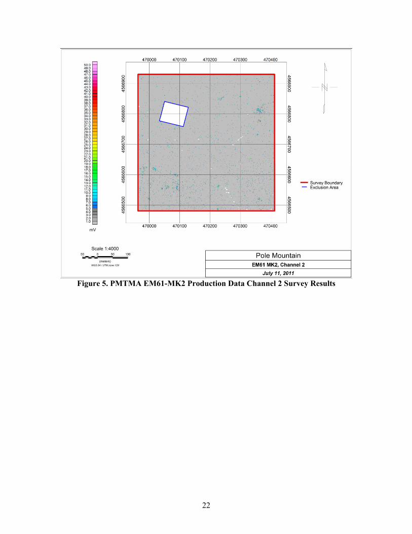
Figure 5 is a plot of the PMTMA EM61-MK2 production survey processed data. The anomaly distribution is relatively uniform throughout with two high density areas located in the northeast and southwest. Targets were picked using a threshold value of 5.2 mV on channel 2, which is equivalent to the theoretical response of a 37mm at 30 cm below ground surface from a standard cart-mounted EM61. A total of 2,370 targets were identified (see Figure 6) with 160 of them being seed items (see Section 7.3).

6.2 METAL MAPPER CUED DATA ANALYSIS AND CLASSIFICATION METHODS

6.2.1 Overview of the Classification Process

Figure 7 is a simplified diagram illustrating the processing flow that transformed target parameters extracted from the MM cued data into decisions about the likelihood that a particular target is ordnance or clutter and, if ordnance, the probable type. Target parameterization was performed as a necessary prerequisite processing step. The flow diagram illustrates the remaining steps:

Rule-Based Analysis (RBA)

Artificial Neural Network (ANN) and Distance Likelihood Ratio Test (DLRT)

Library Curve Matching (LM)

22

Figure 5. PMTMA EM61-MK2 Production Data Channel 2 Survey Results

23

Figure 6. PMTMA EM61-MK2 Production Data with 2,370 Selected Targets and Grid

Frame

24

Figure 7. Simplified Block Diagram Illustrating the Processing Steps

Used to Generate a Prioritized Dig List

6.2.2 Target Parameterization

URS’ approach to discrimination required scalar “features,” or parameters, that are extracted from the principal polarizability curves. These curves were calculated by fitting MM cued data using a point dipole characterization by an anisotropic polarization tensor. These features were also core elements in the RBA and classifiers. URS employed Geosoft’s Oasis Montaj UX-Analyze inversion routines for single and multi-source results to extract the principal polarizability transient curves from the acquired cued MM data. Scalar parameters (features) were derived from the principal polarizability transients for target discrimination. The discrimination features are based on scalar moments of the principal transients as defined by Smith and Lee (2002). The target parameters can broadly be categorized into three categories: size, shape, and time (persistence). Size is measured by two different

methods of integration known as the zero and first moment: dtdtdPP 0 and dt

dtdPtP 1 .There

are eight size scalars: P0x, P0y, P0z, I2(P0), P1x, P1y, P1z, and I2(P1), with I2(P0) defined as √

25

P0xP0yP0z. Shape has six scalars: P0T = √( P0yP0z), P0R = P0x/P0T, P0E = (P0y - P0z)/P0x, P1T, P1R, and P1E. Time (persistence) has four scalars: τx = P1x/P0x, τy = P1y/P0y, τz = P1z/P0z, and τI = I2(P1)/ I2(P0). All the scalar values are internally consistent (i.e., units agree internally).

6.2.3 Rule-Based Decisions

The primary objective of rule-based decisions was to filter the cued data into a set that can be analyzed. The main components consisted of a single/multi-source inversion selection process, a filter logical, a data confidence penalty function, and a target size filter.

6.2.3.1 Single/Multi-Source Inversion Selection

The production data were inverted using Geosoft’s Oasis Montaj UX-Analyze single and multi-source inversion utilities. This generated two sets of parameter values, which required a decision process to select a single data set that characterizes the complete production data (all 2,370 targets). Unlike the single source inversion, multi-source inversion introduced additional targets to the data set (for a total of 2,395 targets). Therefore, as expected, the number of targets increased. URS adopted the pre-existing convention that additional target IDs were named with the acquired ID followed by the extension 00001 or 00002, corresponding to new targets B and C (target A retained the original acquired ID). Upon determining the final target list, only a single target was associated with a single target ID with precedence given to Category 1 then Category 2 then Category 3 and finally Category 0. The decision process is as follows: Eq. (1) If (multi-source targets ==1) Select single source results

Else

If ((Fit_coh_S >= Fit_coh_M) && (P0x != 0)) Select single source results Else If (P0x > 4,500) Select all such multi-source target results Else Select multi-source target with largest P0x results Where; && signifies logical AND || signifies logical OR ! signifies logical NOT The logical equation (1) has three nested if-else statements:

If the multi-source solution identifies only one target, select the single source solution;

If there are multiple targets and the single source inversion fit value is better, select the single source solution;

26

If the single source solution has P0x equal to zero or the multi-source fit value is greater, select all multi-source targets with P0x greater than the 4,500 and else when none exist, select the multi-source target with the largest P0x.

The reason for using this method as opposed to applying the Filter Logical, which incorporates signal amplitude (sa), is that signal amplitude is compromised by a multi-source solution. Signal amplitude no longer reflects the response of a single target and therefore is inadequate as a measure. If the target magnitude as measured by P0x with a response greater than 4,500, the signal amplitude exceeded the lower limit of the filter function, making it exempt from relocation to Category 0. Additionally, the inclusion in the second nested if statement of the term “&& (P0x != 0)” was necessary because the single source inversion output parameter values can be non-zero even though the beta values are zero upon non-convergence.

6.2.3.2 Filter Logical

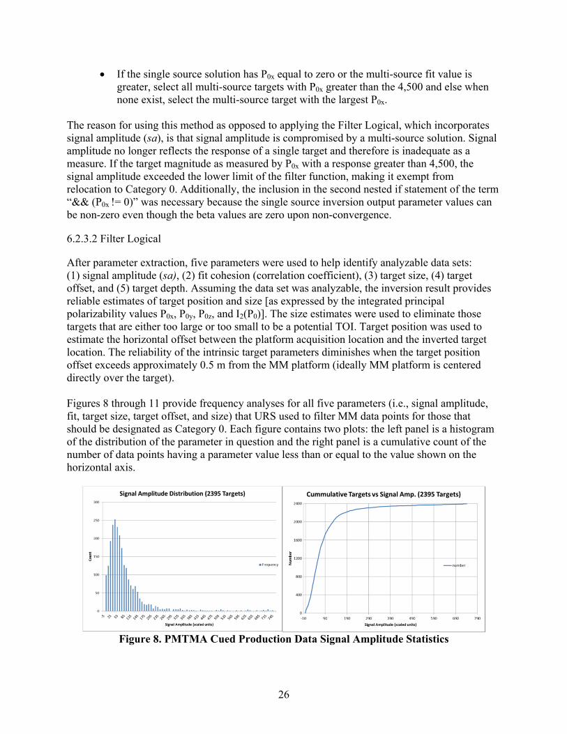
After parameter extraction, five parameters were used to help identify analyzable data sets: (1) signal amplitude (sa), (2) fit cohesion (correlation coefficient), (3) target size, (4) target offset, and (5) target depth. Assuming the data set was analyzable, the inversion result provides reliable estimates of target position and size [as expressed by the integrated principal polarizability values P0x, P0y, P0z, and I2(P0)]. The size estimates were used to eliminate those targets that are either too large or too small to be a potential TOI. Target position was used to estimate the horizontal offset between the platform acquisition location and the inverted target location. The reliability of the intrinsic target parameters diminishes when the target position offset exceeds approximately 0.5 m from the MM platform (ideally MM platform is centered directly over the target). Figures 8 through 11 provide frequency analyses for all five parameters (i.e., signal amplitude, fit, target size, target offset, and size) that URS used to filter MM data points for those that should be designated as Category 0. Each figure contains two plots: the left panel is a histogram of the distribution of the parameter in question and the right panel is a cumulative count of the number of data points having a parameter value less than or equal to the value shown on the horizontal axis.

Figure 8. PMTMA Cued Production Data Signal Amplitude Statistics

27

Figure 9. PMTMA Cued Production Data Fit Statistics

(Cohesion and Correlation Coefficient)

Figure 10. PMTMA Cued Production Data Displacement Statistics

(Horizontal Offset and Depth)

Figure 11. PMTMA Cued Production Data P0x Statistics (Target Size)

Previous ESTCP MM studies (ESTCP 2010) have established that reliable estimates of position and target size are obtained when SNR is >20 (26 dB) and the correlation coefficient (√fit cohesion, see Figure 9) is >0.80. Adjustments were made to accommodate the Geosoft’s Oasis Montaj UX-Analyze parameter signal amplitude, which is the maximum value from the Z

28

receivers with the Z transmitter calculated using the first gate that was selected for the inversion, as opposed to SNR. The cumulative point plots in Figures 8 and 9 show that there were approximately 536 targets with signal amplitude <30 and 85 targets with fit <0.80. When these thresholds are reduced to 10 and 0.75, the number of targets is reduced to 150 and 60, respectively. A penalty function was used to diminish scores for those targets whose signal amplitude and fit fall within the defined penalty zone (see Section 6.2.3.3). In addition, previous studies have established that, when a target is offset from the MM platform center, the ability of the inversion to adequately extract the principal polarizability curves is compromised. In particular, the minor transient symmetry and ratio values can be affected. Previous efforts have found no adverse effects for horizontal offsets <0.5 m, but larger offsets can be affected and should be penalized. There is a maximum offset, at approximately 1.25 m, where targets should be designated as Category 0. For this demonstration, a rule was adopted for not Category 0 targets based on the five parameters (signal amplitude, fit cohesion, target size, target offset, and target depth) as follows: Eq. (2) {(fit > 0.75) && (sa > 20) && (offset < 1.25 m) && !(fit > 0.90)} || {(fit > 0.9)} ||

{(sa >10) && (offset < 0.7 m) && (depth < 0.25 m) && (P0x < lower 95% confidence limit TOI)}

Where: && signifies logical AND || signifies logical OR ! signifies logical NOT The rule identifying not Category 0 targets was extended using fit >0.75 and sa >20 by writing a three-term logical OR equation (2) in order to allow for the three scenarios as follows:

Term 1: Provided fit >0.75 AND sa >20, this term identifies the data point as analyzable (Categories 1–3) when the estimated target offset is <1.25 m AND there is no data point with high fit.

Term 2: This term permits data points with high fit to be defined as analyzable. It is tied to the Term 1 NOT statement.

Term 3: If fit >0.75 and sa >10 then this term identifies points having low offset (>0.7 m), small size (P0x < lower 95% confidence limit TOI), and shallow depth (<0.25 m). Under these conditions, a lower threshold of sa equal to 10 is acceptable. This term allows small clutter to be excluded from Category 0.

When the rule in equation (2) was applied to the 2,395 cued targets, 103 data points (≈4.5%) were identified as Category 0.

29

In an effort to minimize the number of data points immediately placed into Category 0, a two-stage approach to screening the data was adopted. In equation (2), the thresholds were set low for signal amplitude and fit in order to pass more targets into the analyzable category. Then, a multiplicative data confidence penalty function (Ma) was applied that is dependent on signal amplitude and fit parameters to the output of the discriminator (ANN and DLRT). The penalty function was designed to decrease the confidence level of a discrimination decision but not its category designation. The penalty function is discussed in Section 6.2.3.3. Upon examining the data to better understand the large percentage of Category 0 points, it was discovered that many of these targets have very small signal amplitude (<10) and very poor fit (<0.7). After inspecting the EM61 data, it was determined that many of these target responses have an unusually small footprint (i.e., responses on a single data track line with a line spacing of 0.5 m). Targets resulting from small ISO objects and 37mm munitions have footprints that, at a minimum, have a response on two or more data track lines. As the target gets deeper the response is less peaked, and even if the signal is just above the threshold on one line there is still a response just below the threshold on an adjacent line. The deeper a horizontal ISO gets the more point-like its response (the far field response is point-like). Table 3 illustrates the response of small TOIs over multiple data track lines.

Table 3. Multi-Line Response of Some Small Items Type (tentative) Target ID EM61 Grid Value Number Lines

37mm 1229 19.5 4 37mm 1029 20.6 4 37mm 1595 7.9 2 37mm 2179 7.2 3 37mm 1365 23.7 4 37mm 1952 17.3 4 37mm 1472 16.3 3 37mm 2154 9.7 2 37mm 1902 17.2 3 37mm 2330 19.1 3 ISO 2290 15.3 3 ISO 1679 18.2 3 ISO 2057 17.5 3 ISO 1268 17.3 4 ISO 1860 16.7 4 ISO 567 14 2 ISO 572 9.1 2 ISO 1844 23.7 3 ISO 1011 11.3 3 ISO 2132 16.9 3

The cued static results supported that no metallic source exists at these locations. These responses appeared to be an EM61 noise issue. It was estimated that approximately 50% of these targets (noise files) could be moved to Category 2 by using the simple criterion that, if the target footprint is on a single data track line and sa <10, then move to Category 2. The number of category points was reduced to ≈2.3%, which is more in line with previous MM surveys.

30

6.2.3.3 Data Confidence Penalty Function

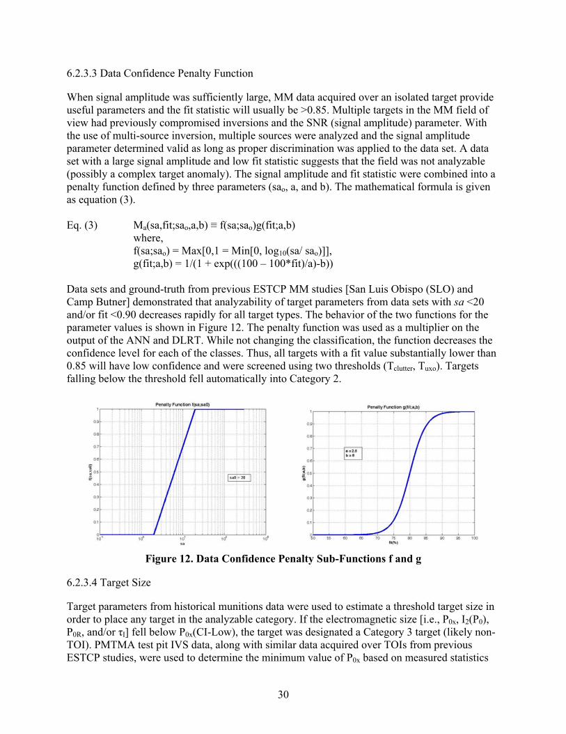
When signal amplitude was sufficiently large, MM data acquired over an isolated target provide useful parameters and the fit statistic will usually be >0.85. Multiple targets in the MM field of view had previously compromised inversions and the SNR (signal amplitude) parameter. With the use of multi-source inversion, multiple sources were analyzed and the signal amplitude parameter determined valid as long as proper discrimination was applied to the data set. A data set with a large signal amplitude and low fit statistic suggests that the field was not analyzable (possibly a complex target anomaly). The signal amplitude and fit statistic were combined into a penalty function defined by three parameters (sao, a, and b). The mathematical formula is given as equation (3). Eq. (3) Ma(sa,fit;sao,a,b) ≡ f(sa;sao)g(fit;a,b) where, f(sa;sao) = Max[0,1 = Min[0, log10(sa/ sao)]], g(fit;a,b) = 1/(1 + exp(((100 – 100*fit)/a)-b)) Data sets and ground-truth from previous ESTCP MM studies [San Luis Obispo (SLO) and Camp Butner] demonstrated that analyzability of target parameters from data sets with sa <20 and/or fit <0.90 decreases rapidly for all target types. The behavior of the two functions for the parameter values is shown in Figure 12. The penalty function was used as a multiplier on the output of the ANN and DLRT. While not changing the classification, the function decreases the confidence level for each of the classes. Thus, all targets with a fit value substantially lower than 0.85 will have low confidence and were screened using two thresholds (Tclutter, Tuxo). Targets falling below the threshold fell automatically into Category 2.

Figure 12. Data Confidence Penalty Sub-Functions f and g

6.2.3.4 Target Size

Target parameters from historical munitions data were used to estimate a threshold target size in order to place any target in the analyzable category. If the electromagnetic size [i.e., P0x, I2(P0), P0R, and/or τI] fell below P0x(CI-Low), the target was designated a Category 3 target (likely non-TOI). PMTMA test pit IVS data, along with similar data acquired over TOIs from previous ESTCP studies, were used to determine the minimum value of P0x based on measured statistics

31

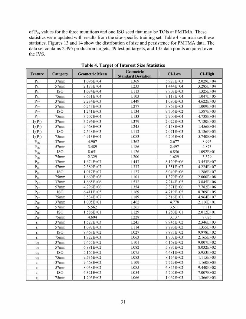
of P0x values for the three munitions and one ISO seed that may be TOIs at PMTMA. These statistics were updated with results from the site-specific training set. Table 4 summarizes these statistics. Figures 13 and 14 show the distribution of size and persistence for PMTMA data. The data set contains 2,395 production targets, 49 test pit targets, and 135 data points acquired over the IVS.

Table 4. Target of Interest Size Statistics

Feature Category Geometric Mean Geometric

Standard Deviation CI-Low CI-High

P0x 37mm 1.096E+04 1.369 5.923E+03 2.029E+04 P0x 57mm 2.178E+04 1.233 1.444E+04 3.285E+04 P0x ISO 1.074E+04 1.113 8.703E+03 1.325E+04 P0x 75mm 8.631E+04 1.103 7.118E+04 1.047E+05 P0T 37mm 2.234E+03 1.449 1.080E+03 4.622E+03 P0T 57mm 6.243E+03 1.277 3.863E+03 1.009E+04 P0T ISO 1.241E+03 1.134 9.706E+02 1.587E+03 P0T 75mm 3.707E+04 1.133 2.900E+04 4.738E+04

I2(P0) 37mm 3.796E+03 1.379 2.022E+03 7.130E+03 I2(P0) 57mm 9.468E+03 1.245 6.158E+03 1.456E+04 I2(P0) ISO 2.548E+03 1.112 2.071E+03 3.136E+03 I2(P0) 75mm 4.913E+04 1.083 4.205E+04 5.740E+04 P0R 37mm 4.907 1.362 2.677 8.993 P0R 57mm 3.489 1.186 2.497 4.873 P0R ISO 8.651 1.126 6.856 1.092E+01 P0R 75mm 2.329 1.200 1.629 3.329 P1x 37mm 1.674E+07 1.447 8.120E+06 3.453E+07 P1x 57mm 2.389E+07 1.337 1.351E+07 4.224E+07 P1x ISO 1.017E+07 1.127 8.040E+06 1.286E+07 P1x 75mm 1.660E+08 1.101 1.370E+08 2.000E+08 P1T 37mm 1.665E+06 1.532 7.214E+05 3.845E+06 P1T 57mm 4.296E+06 1.354 2.371E+06 7.782E+06 P1T ISO 6.411E+05 1.169 4.719E+05 8.709E+05 P1T 75mm 3.534E+07 1.189 2.516E+07 4.964E+07 P1R 37mm 1.005E+01 1.462 4.778 2.116E+01 P1R 57mm 5.562 1.265 3.511 8.811 P1R ISO 1.586E+01 1.129 1.250E+01 2.012E+01 P1R 75mm 4.694 1.228 3.137 7.025 τx 37mm 1.527E+03 1.245 9.945E+02 2.346E+03 τx 57mm 1.097E+03 1.114 8.880E+02 1.355E+03 τx ISO 9.468E+02 1.027 8.983E+02 9.978E+02 τx 75mm 1.922E+03 1.063 1.707E+03 2.165E+03 τIT 37mm 7.455E+02 1.101 6.169E+02 9.007E+02 τIT 57mm 6.881E+02 1.082 5.895E+02 8.032E+02 τIT ISO 5.165E+02 1.075 4.481E+02 5.953E+02 τIT 75mm 9.536E+02 1.083 8.154E+02 1.115E+03 τI 37mm 9.468E+02 1.109 7.729E+02 1.160E+03 τI 57mm 8.038E+02 1.085 6.845E+02 9.440E+02 τI ISO 6.321E+02 1.054 5.702E+02 7.007E+02 τI 75mm 1.205E+03 1.066 1.062E+03 1.366E+03

32

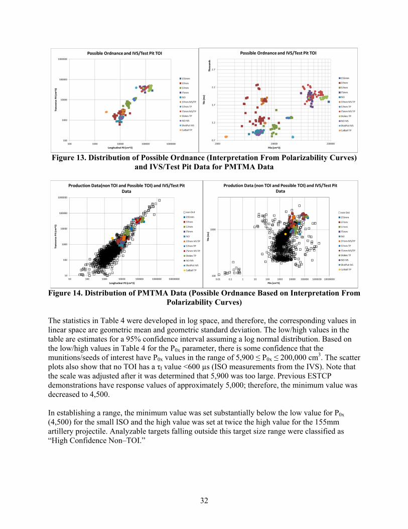
Figure 13. Distribution of Possible Ordnance (Interpretation From Polarizability Curves)

and IVS/Test Pit Data for PMTMA Data

Figure 14. Distribution of PMTMA Data (Possible Ordnance Based on Interpretation From

Polarizability Curves) The statistics in Table 4 were developed in log space, and therefore, the corresponding values in linear space are geometric mean and geometric standard deviation. The low/high values in the table are estimates for a 95% confidence interval assuming a log normal distribution. Based on the low/high values in Table 4 for the P0x parameter, there is some confidence that the munitions/seeds of interest have P0x values in the range of 5,900 ≤ P0x ≤ 200,000 cm3. The scatter plots also show that no TOI has a τI value <600 µs (ISO measurements from the IVS). Note that the scale was adjusted after it was determined that 5,900 was too large. Previous ESTCP demonstrations have response values of approximately 5,000; therefore, the minimum value was decreased to 4,500. In establishing a range, the minimum value was set substantially below the low value for P0x (4,500) for the small ISO and the high value was set at twice the high value for the 155mm artillery projectile. Analyzable targets falling outside this target size range were classified as “High Confidence Non–TOI.”

33

6.2.4 Classifiers (Target of Interest Indicator Tools)

The commercial software package Statistica version 9.0 was used to select and train the ANN for discrimination. Additionally MATLAB’s statistical package was employed for the DLRT analysis as well as many supportive calculations.

6.2.4.1 Data

For preliminary training purposes, polarizability parameters from over 700 cued MM data points from four previous studies (Yuma, Aberdeen, SLO, and Camp Butner) in conjunction with the PMTMA survey were assembled. The 15 polarizability parameters examined are identified in Section 6.2.4.3. URS experimented with various subsets of the 15-feature vector, which were determined using principal component analysis to determine those most suitable for the ANN analysis. The best solution employed all 15 scalars of the feature vector. While overtraining can be a problem, tentative results were acceptable using the hybrid classifier. This consists of a much more restrictive (localized cluster) with the first pass classifier (ANN) because the second pass classifier (DLRT) is considerably less restrictive. The space dimension is reduced (based on the importance of the feature attributes in the ANN) and then the two variable parameters that can be customized (nearest neighbor number and a distance measure) to control cluster expansion. The PMTMA data set had good separation in size, shape, and time (see Figures 13 and 14) based on a visual assessment of the polarization curves. This implies that a large feature vector should perform well. Previous studies have shown that the best parameters for discrimination are parameters related to size and time (persistence), but shape can also be useful. Under ideal conditions, shape is clearly a distinguishing characteristic with the two minor (transverse) polarizability curves nearly identical, and one larger major (longitudinal) polarizability curve leading to P0R > 1 and P0E << 1. Unfortunately, many munitions-like targets emulate this classic polarizability structure, in particular, small frag with large aspect ratios. In addition, low signal amplitude, large lateral offsets, and unfavorable target pitch attitude often compromise the quality of the inversion, resulting in minor polarizability curves that separate, generating less favorable P0R and P0E values.

6.2.4.2 Training Data

After performing the preliminary analysis, the trained ANN was applied to the PMTMA production data, which yielded more false negative and ambiguous results than desired. False negative results were determined based on a contradictory ANN classification relative to the visual assessment of the polarization curve. Ambiguous results were given an ANN value near the decision surface, yet with equivalent classification. Subsequent analysis resulted in the list of training targets submitted to the ESTCP Program Office. All training targets had munitions-like characteristics such as representative cluster features, LM to 20mm, and low eccentricity. Over 54% (26 of the 46) had P0x parameter values below the 4,500 Category 3 threshold in order to reduce the risk of missing TOI smaller than 37mm projectiles, the smallest known ordnance on-site. The submitted training data list is contained in the Primary Score Spreadsheet in Appendix E. Training data have a dig threshold category number of -1.

34

6.2.4.3 Artificial Neural Network Classifier

The initial ANN classification effort included training and evaluating networks using feature vectors with 3, 5, 9, 12, and 15 features. URS selected a 15 feature vector because its overall performance exceeded those of smaller dimensions. Table 5 displays the five best trained networks. Network 3 (15-6-2) was selected due to its overall performance in minimizing false negatives. The number of false negative is relative to the visual identification of the polarization curves, which placed suspect curves in Category 1. Figure 15 shows receiver operating characteristic (ROC) curves for the five best trained ANN. This data set included 2,384 targets because URS removed 11 duplicate targets.

Table 5. Five Best Trained ANN Results Class-0 Class-1 Class-All 1.MLP 15-13-2 Total 2115.000 269.0000 2384.000 Correct 2092.000 173.0000 2265.000 Incorrect 23.000 96.0000 119.000 Correct (%) 98.913 64.3123 95.008 Incorrect (%) 1.087 35.6877 4.9922.MLP 15-6-2 Total 2115.000 269.0000 2384.000 Correct 2094.000 182.0000 2276.000 Incorrect 21.000 87.0000 108.000 Correct (%) 99.007 67.6580 95.470 Incorrect (%) 0.993 32.3420 4.5303.MLP 15-6-2 Total 2115.000 269.0000 2384.000 Correct 2056.000 179.0000 2235.000 Incorrect 59.000 90.0000 149.000 Correct (%) 97.210 66.5428 93.750 Incorrect (%) 2.790 33.4572 6.2504.MLP 15-13-2 Total 2115.000 269.0000 2384.000 Correct 2087.000 163.0000 2250.000 Incorrect 28.000 106.0000 134.000 Correct (%) 98.676 60.5948 94.379 Incorrect (%) 1.324 39.4052 5.6215.MLP 15-13-2 Total 2115.000 269.0000 2384.000 Correct 2087.000 182.0000 2269.000 Incorrect 28.000 87.0000 115.000 Correct (%) 98.676 67.6580 95.176 Incorrect (%) 1.324 32.3420 4.824

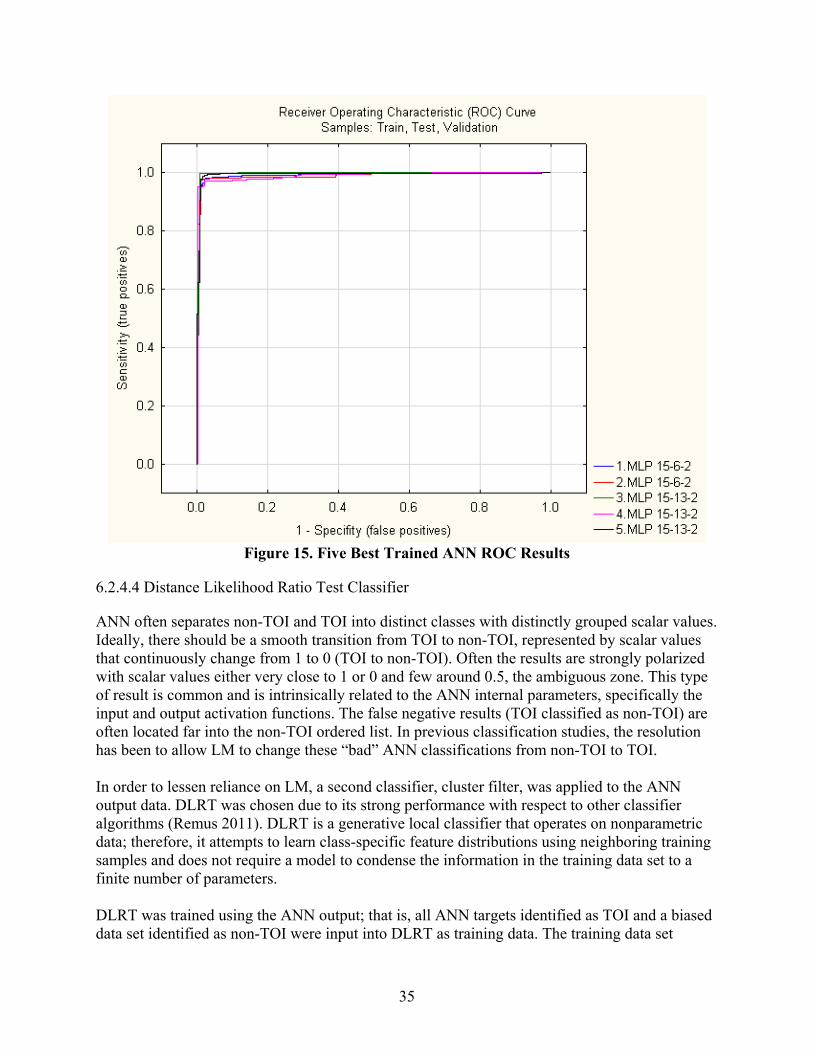
35

Figure 15. Five Best Trained ANN ROC Results

6.2.4.4 Distance Likelihood Ratio Test Classifier

ANN often separates non-TOI and TOI into distinct classes with distinctly grouped scalar values. Ideally, there should be a smooth transition from TOI to non-TOI, represented by scalar values that continuously change from 1 to 0 (TOI to non-TOI). Often the results are strongly polarized with scalar values either very close to 1 or 0 and few around 0.5, the ambiguous zone. This type of result is common and is intrinsically related to the ANN internal parameters, specifically the input and output activation functions. The false negative results (TOI classified as non-TOI) are often located far into the non-TOI ordered list. In previous classification studies, the resolution has been to allow LM to change these “bad” ANN classifications from non-TOI to TOI. In order to lessen reliance on LM, a second classifier, cluster filter, was applied to the ANN output data. DLRT was chosen due to its strong performance with respect to other classifier algorithms (Remus 2011). DLRT is a generative local classifier that operates on nonparametric data; therefore, it attempts to learn class-specific feature distributions using neighboring training samples and does not require a model to condense the information in the training data set to a finite number of parameters. DLRT was trained using the ANN output; that is, all ANN targets identified as TOI and a biased data set identified as non-TOI were input into DLRT as training data. The training data set

36

included 428 ANN output targets with 224 identified as TOI and 204 as non-TOI. DLRT then operated on the remaining data, 1,956 targets, as test data. Additional controlled parameters were input feature scalars and the number of neighbors. URS selected P0x, P0E, P1x, P1r, and τ0x because these features have the largest Eigen Values in a Principle Component Analysis. The nearest neighbor parameter was determined based on leveling the number of TOI identified (see Table 6). URS selected a nearest neighbor number of 9. Figure 16 is the DLRT output result Scatter Plot, P0x vs τ0x. The figure shows the ANN input training data with red and green circles and the DLRT results with black, blue, and purple squares. Both the blue and purple squares are in close proximity to the ANN TOI with the purple squares being closer. The purple squares are the first 50 DLRT TOI identified and have a larger distance measure relative to the blue squares, DLRT TOI targets 51–132, which means they are closer to the ANN TOI. Shown is a single scatter plot, so the apparent distance can be misleading. The cutoff of 50 was based on an assessment of potential TOI from a visual assessment of the polarization curves.

Table 6. DLRT Nearest Neighbor Identified TOI Number of Nearest Neighbors 1 2 3 4 5 6 7 8 9 10 Number of DLRT Identified as TOI 184 141 154 160 152 143 136 134 132 132

Figure 16. DLRT Output Results Scatter Plot, P0x vs τ0x

37

6.2.4.5 Library Matching Classifier

URS applied LM in a subordinate role in analyzing the PMTMA data. The matching algorithm was run on all analyzable data targets. Then the discrimination scores were examined from both the ANN/DLRT and LM. A good library match indicated a Category 1 target. However, a poor match could suggest either non-TOI or possibly TOI not represented in the target type library. LM overrode the ANN/DLRT score in all cases where the LM score indicated Category 1, while ANN/DLRT indicates Category 3 or 2. This approach moved a few targets from Categories 3 and 2 to Category 1 in a principled manner. Classification used the Geosoft’s Oasis Montaj UX-Analyze LM algorithm, which compares the derived polarizabilities with a library of known target signatures. Three weighted parameters were selected to create the final metric: the amplitude of the primary polarizability (β 1), and two shape parameters calculated from the ratio of the second and third polarizability to the first (β 2 /β 1 and β 3 /β 1). The difference in the values was computed at all-time gates, excluding those where the values were negative. The differences were then plugged into a Gaussian function. The “time constants” in these Gaussians functions were derived by examining the variability in the amplitude and shape parameters for a large number of objects for which ground truth is known. Medians were taken to avoid bad data points. Finally, the results were averaged, producing a metric that ranges from 0 (worst possible fit) to 1 (perfect fit). Note that the procedure just described is not a library constrained match (i.e., UX-Analyze does not invert the data, forcing the β’s to be those of each library object in turn, but rather compares the unconstrained polarizabilities to those of the library). As such, the comparison ran rapidly, and there was no need to reduce the number of separate types in the library to balance computation time. In fact, URS tried many different derived libraries and weighted fits. URS applied LM to the training/production data. The training data included all PMTMA IVS and test pit data (see Figure 17), as well as all relevant SLO data that were acquired during the National Association of Ordnance Contractors workshop. The only SLO data used were for documented PMTMA ordnance. But, LM was applied to 20mm targets and the best matches used as training data in order to minimize missing any potential targets smaller than 37mm. URS applied a bias weight to the LM; the amplitude metric (β 1) received a weight of 50%, the first shape metric (β 2 /β 1) received a weight of 33.33%, and the second shape metric (β 3 /β 1) received a weight of 16.66%. Based on prior experience, it is not uncommon to have a large eccentricity for an ordnance item. As previously stated, URS used LM as secondary, in that it served to override poor decisions of the classifiers (ANN and DLRT) and in a principled way to move a few targets from Categories 3 and 2 to Category 1.

6.2.5 Data Products

URS submitted four related prioritized target lists. Prior to following the above procedures to generate these lists, URS reduced the number of targets from 2,384 to 2,370; that is, only a single target was associated with a single target ID with precedence given to Category 1 then Category 2 then Category 3 and finally Category 0. Three target lists differed only in the number of targets placed in Category 1 and Category 2. The overall strategy was to use a hybrid classifier that used the output of one classifier (ANN) as the input of another (DLRT). LM was then applied as a means of moving a few misidentified targets from Category 2 or 3 to Category 1.

38

Figure 17. LM of Historic Ordnance Documented at PMTMA

For target list 1, NnLMCa, URS used only the ANN and LM classifiers. Category 1 targets were identified by these two classifiers only (DLRT was not applied). For target list 2, NnLmDLRTsCa, the ANN, DLRT short TOI list, and LM were used to identify Category 1 targets. The short version of DLRT used a TOI cutoff of 50 targets based on an assessment (visual interpretation of the polarization curves) of where Category 1 targets ended. For target

39

list 3, NnLmDLRTlCa, the ANN, DLRT full TOI list (based on a distance metric), and LM were used to identify the Category 1 targets. For each of these lists, 1 through 3, the reduced Category 0 target list was used. Target list 4, NnLmDLRTl, is identical to target list 3 except the reduced Category 0 list was not used; that is, all Category 0 targets were to be dug. This was considered the safe list. Table 7 provides the general prioritized target list statistics. The complete prioritized target lists are contained in Appendix F.

Table 7. General Target List Statistics

List Name TOI TOI

Identified (%)

Training Targets

Training Targets

(%)

Can’t Analyze

Can’t Analyze

(%)

List Length

List Length

(%)

Total Targets

NnLmCa 160 100 46 1.9 51 2.2 409 17.2 2370 NnLmDLRTsCa 160 100 46 1.9 51 2.2 430 18.1 2370 NnLmDLRTICa 160 100 46 1.9 51 2.2 477 20.1 2370 NnLmDLRTl 160 100 46 1.9 107 4.5 533 22.5 2370

URS prioritized target lists identified all TOI in Category 1 (see Figures 18 through 21). Table 7 contains general statistics. The ANN and LM identified all TOI; therefore, the hybrid classifier, which used DLRT as the second tier classifier, necessarily identified all the TOI. All target lists used the same training data and a minimum Category 0 list. One list used the full Category 0 list. The training data and Category 0 list accounted for a minimum of 4.1% and a maximum of 6.4% of the targets.

Figure 18. ANN, LM, and Short Category 0 List

40

Figure 19. ANN, DLRT Short, LM, and Short Category 0 List

Figure 20. ANN, DLRT Long, LM, and Short Category 0 List

41

Figure 21. ANN, DLRT Long, LM, and Long Category 0 List

42

7.0 PERFORMANCE ASSESSMENT

The performance objectives for this demonstration are summarized in Table 1 and are repeated here as Table 8. The results for each criterion are discussed in the following sections.

Table 8. Quantitative Performance Objectives for This Demonstration Performance

Objective Metric Data Required Success Criteria Results

EM61-MK2 Data Collection Objectives

Along-line measurement spacing

Point-to-point spacing from data set

Mapped production survey data

90% <15 cm along-line spacing

Data quality objective (DQO) achieved with exception noted in Section 7.1.4

Complete coverage of the demonstration site

Footprint coverage Mapped production survey data

≥85% coverage at 0.5 m line spacing and ≥98% coverage at 0.75 m line spacing calculated using UX-Process Footprint Coverage QC Tool

DQO achieved

Detection of all TOI Percent detected of seeded items

Location of seeded items and anomaly list

100% of seeded items detected

DQO achieved

MM Data Analysis and Classification Objectives

Maximize correct classification of TOI

Percent of TOI placed in Category 1

Prioritized anomaly lists and dig results

Correctly classify 100% of TOI

DQO achieved

Maximize correct classification of non-TOI

Percent of correctly classified non-TOI

Prioritized anomaly lists and dig results

>65% of non-TOI classified in Category 3

DQO achieved

Specification of no-dig threshold

Percent of TOI placed in Categories 1 or 2 and percent of non-TOI placed in Category 3.

MM cued data, prioritized anomaly lists, and dig results

100% of TOI placed in Categories 1 and 2 and >65% of non-TOI placed in Category 3.

DQO achieved

Minimize number of anomalies that cannot be analyzed

Percentage of anomalies classified as Category 0

Inverted MM cued data and prioritized anomaly dig list

Reliable target parameters can be estimated for >95% of anomalies on each sensor’s detection list

DQO achieved

Category 0 targets are categorized correctly

The polarization curves visually reflect a non-analyzable target

Inverted MM cued data and polarization curves

All targets placed in the “Can’t Analyze” category will have polarization curves reflecting a non-analyzable target.

DQO achieved

Correctly extract feature scalars

Category 1 TOI should cluster in various feature space scatter plots

Derived target feature vectors, inverted MM cued data, and polarization curves

Various feature space scatter plots display distinct clustering

DQO achieved

43

Performance Objective

Metric Data Required Success Criteria Results

Correctly classify Category 2 targets

Category 2 targets should display TOI-like properties

Polarization curves, derived target feature vectors, and dig results

Category 2 targets should be proximal to TOI clusters and/or polarization curves display TOI characteristics

DQO achieved

7.1 OBJECTIVE: ALONG-LINE MEASUREMENT SPACING

Down-line data must be sufficiently dense to support detection of all anomalies and minimal data gaps.

7.1.1 Metric

Along track point-to-point data spacing is measured using EM61 MK2 RTK GPS point positioning.

7.1.2 Data Requirements

Mapped production survey data.

7.1.3 Success Criteria

Ninety percent of the production data will have a point-to-point displacement of <0.15 m.

7.1.4 Results

URS utilized Geosoft’s Oasis Montaj UX-Process Sample Separation analysis module. The separation distance was set to 0.15 m, and 1.9% of the data exceeded that displacement, which is much lower than the required 10%. This includes end-of-line points; therefore, the actual percentage is much lower than the displayed value. Also note that the flagged points are relatively large, making them more prominent than they are (the point size and line labels are internally set by the program and cannot be altered by the user). Data collected on June 22 and June 23, 2011, by Team 2 did not meet this metric. Data were collected using an older DOS-based Allegro field computer. The acquisition software for Allegro does not collect data at uniform time windows; some responses may be 0.2 seconds to 0.3 seconds apart instead of the specified 0.1 seconds. During dynamic acquisition at a walking pace, this resulted in 15% to 20% of the down-line sample separations exceeding the 0.15 m metric. This problem was resolved in later data collection by replacing the Allegro with a newer Windows CE-based model, and it was decided to keep the data after coordination with ESTCP. All seeded TOIs in the affected area were detected and properly targeted.

44

7.2 OBJECTIVE: COMPLETE COVERAGE OF THE DEMONSTRATION SITE

The EM61-MK2 baseline data were used to identify metallic anomalies on the demonstration site for further analysis. Therefore, the expectation was complete mapping of the accessible areas of the site.

7.2.1 Metric

Percent coverage of the demonstration site with the mapped production survey data.

7.2.2 Data Requirements

Mapped production survey data used to generate grids to allow target picking.

7.2.3 Success Criteria

Greater than 85% coverage at 0.5 m line spacing and greater than 98% coverage at 0.75 m line spacing are calculated using UX Process Footprint Coverage QC Tool.

7.2.4 Results

URS utilized Geosoft’s Oasis Montaj UX-Process Footprint Coverage QC Tool. The available area for the geophysical survey is 48.7 acres, which includes the non-exclusion area. Using a 0.5 m width footprint, the analysis determined that 90.41% of the area was covered (see Figure 23), and using a 0.75 m width footprint the analysis determined that 99.62% was covered (see Figure 24). This exceeds the required 85% and 98% for the 0.5 m and 0.75 m width footprint, respectively.

45

Figure 22. PMTMA Footprint Coverage Plot Using a Width of 0.5 m

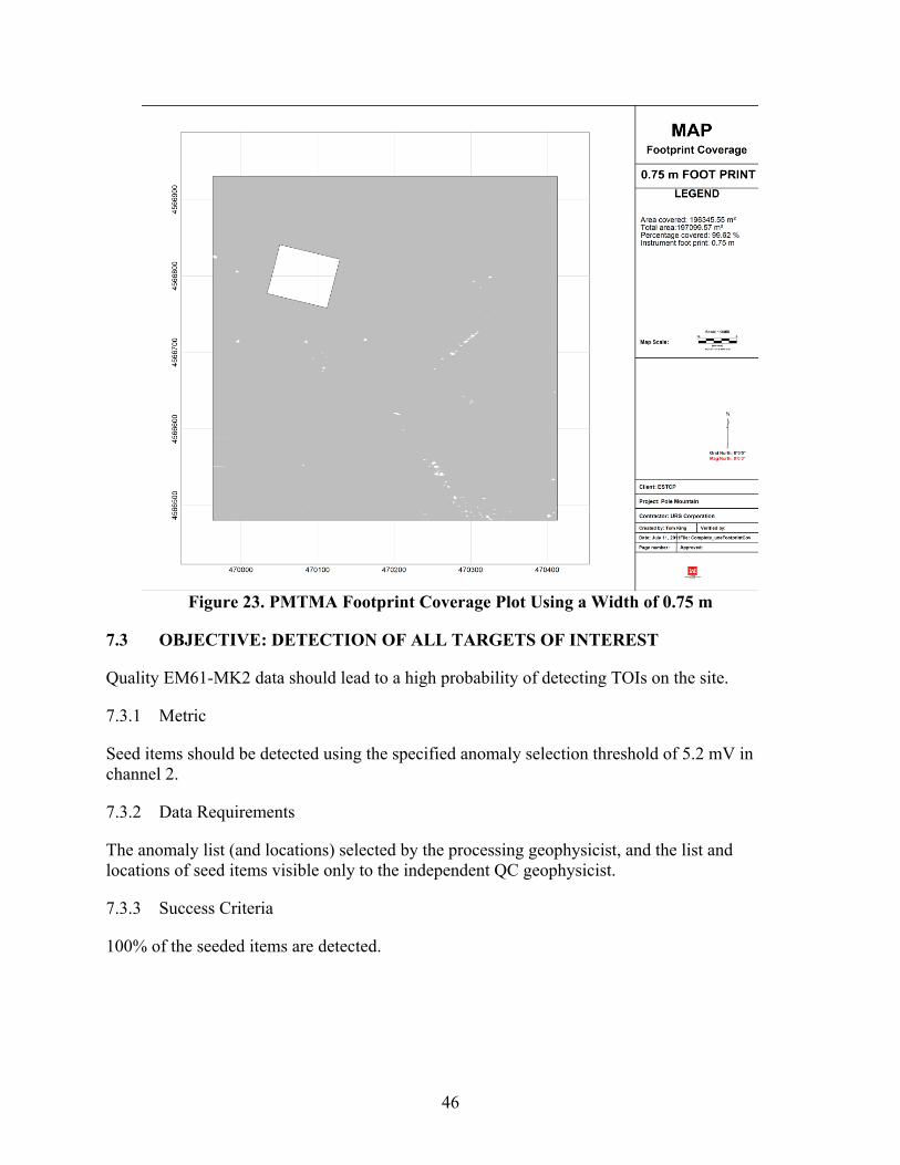
46

Figure 23. PMTMA Footprint Coverage Plot Using a Width of 0.75 m

7.3 OBJECTIVE: DETECTION OF ALL TARGETS OF INTEREST

Quality EM61-MK2 data should lead to a high probability of detecting TOIs on the site.

7.3.1 Metric

Seed items should be detected using the specified anomaly selection threshold of 5.2 mV in channel 2.

7.3.2 Data Requirements

The anomaly list (and locations) selected by the processing geophysicist, and the list and locations of seed items visible only to the independent QC geophysicist.

7.3.3 Success Criteria

100% of the seeded items are detected.

47

7.3.4 Results

The independent QC geophysicist identified all 160 QC seed items (see Figure 25) placed on the target list delivered to the ESTCP Program Office. Appendix C contains a table listing the QC seed ID, description, easting, and northing.

Figure 24. PMTMA EM61-MK2 Production Data With All 160 QC Seed Items Identified

7.4 OBJECTIVE: MAXIMIZE CORRECT CLASSIFICATION OF TARGETS OF INTEREST

The objective was to correctly classify TOI.

7.4.1 Metric

Percentage of TOI correctly classified as Category 1 using each classification approach.

7.4.2 Data Requirements

Prioritized dig list for each classification approach using provided target list in conjunction with a classification strategy. Results of validation digging.

48

7.4.3 Success Criteria

Each classification approach should correctly identify all TOI in Category 1.

7.4.4 Results

All TOIs were identified on all four submitted prioritized target lists within Category 1 (see ROC curves in Figures 18 through 21).

7.5 OBJECTIVE: MAXIMIZE CORRECT CLASSIFICATION OF NON-TARGETS OF INTEREST

The objective was to correctly classify non-TOI.

7.5.1 Metric

Percentage of correctly classified non-TOI using each classification approach.

7.5.2 Data Requirements

Prioritized dig list for each classification approach using provided target list in conjunction with a classification strategy. Results of validation digging.

7.5.3 Success Criteria

Greater than 65% of non-TOI classified in Category 3.

7.5.4 Results

Table 9 presents the results for this objective. All four submitted lists achieved the DQOs.

Table 9. Minimization of Non-TOI Results

List Name Training Can't

Analyze Category 1

Category 2 and 3

Dig No Dig Dig/No

Dig Dig/No Dig

(%) NnLmCa 46 51 312 1961 409 1961 0.2086 20.86

NnLmDLRTsCa 46 51 333 1940 430 1940 0.2216 22.16 NnLmDLRTlCa 46 51 380 1893 477 1893 0.2520 25.20

NnLmDLRTl 46 107 436 1837 533 1837 0.2901 29.01

7.6 OBJECTIVE: SPECIFICATION OF NO-DIG THRESHOLD

To correctly establish the dig/no-dig threshold, URS isolated those targets nearest to the ANN (first classifier of the hybrid classifier) TOI using a nearest neighbor method, based on the value of the nearest neighbor parameter (second classifier of the hybrid classifier) and by reducing the dimensions of feature space to those most prominent through a PCA analysis.

49

7.6.1 Metric

Percent of TOI placed in Categories 1 or 2 and percent of non-TOI placed in Category 3.

7.6.2 Data Requirements

Prioritized anomaly lists and results of validation digging.

7.6.3 Success Criteria

100% of TOI are identified in Categories 1 and 2 and greater than 65% of non-TOI are identified in Category 3.

7.6.4 Results

DQO achieved.

7.7 OBJECTIVE: MINIMIZE NUMBER OF ANOMALIES THAT CANNOT BE ANALYZED

The objective as to minimize the number of anomalies that cannot be analyzed.

7.7.1 Metric

The percentage of targets classified as Category 0.

7.7.2 Data Requirements

Inverted MM cued data and prioritized anomaly lists.

7.7.3 Success Criteria

Less than 5% of the anomalies are Category 0.

7.7.4 Results

Five percent can be reduced to 1% or less. The initial Category 0 algorithm is that the inversion correlation coefficient should be greater than 0.75, the signal amplitude <20 dB, and the MM platform/inversion target location displacement <0.5 m. Unfortunately, this presupposes the presence of a measurable target. URS found that many of the identified targets were anomalous EM61 responses. Therefore, the original EM61 data were reevaluated and a target footprint analysis performed (see Figure 25 and Table 3) to reduce the number of Category 0 targets from 4.7% to 2.3%, which is more in line with previous studies. Targets with EM61 responses on a single transect profile and with MM static “noise” responses were determined analyzable. Figure 25 shows Targets 2154 and 2330 (37mm) and targets 2132 and 2057 (ISOs, the smallest documented project TOI). All four have a footprint covering at least 0.5 m, the line spacing.

50

Figure 25. Footprints of targets 2154 and 2330 (37mm) and targets 2132 and 2057 (ISOs)

7.8 OBJECTIVE: CORRECTLY CLASSIFY CATEGORY 0 TARGETS

The objective was to verify that Category 0 targets are correctly classified.

7.8.1 Metric

Percent of polarization curves in Category 0 that visually reflect a non-analyzable target.

7.8.2 Data Requirements

Inverted MM cued data and the polarization curves.

7.8.3 Success Criteria

All targets placed in Category 0 will have polarization curves reflecting a non-analyzable target.

7.8.4 Results

All target polarization curves placed in Category 0 have polarization curves that were extremely noisy, response below the measurable limits, responses above the measurable limit, negative beta values (that are displayed graphically as positive), etc.

7.9 OBJECTIVE: CORRECTLY EXTRACT FEATURE SCALARS

The objective was to correctly extract the feature scalars for the MM cued inversion results.

51

7.9.1 Metric

Category 1 TOI should cluster in various feature space scatter plots.

7.9.2 Data Requirements

Inverted MM cued inversion results, polarization curves, and derived features scalars.

7.9.3 Success Criteria

Various feature space scatter plots for TOI will display distinct clustering.

7.9.4 Results

URS verified that similar TOIs plotted in clusters and visually verified that the polarization curves similarly reflected TOIs.

7.10 OBJECTIVE: CORRECTLY CLASSIFY CATEGORY 2 TARGETS

The objective was to verify that Category 2 targets are correctly classified.

7.10.1 Metric

Category 2 feature scalars should visually plot closely to Category 1 targets.

7.10.2 Data Requirements

Derived feature scalars, polarization curves, and validation digging results.

7.10.3 Success Criteria

Category 2 targets should be proximal to TOI clusters and/or polarization curves should display TOI characteristics.

7.10.4 Results

Visually, most scatter plots display a close proximal relationship between Category 2 targets and TOI clusters. In complement, many of the Category 2 targets had classification values just outside the decision surface, close to but <0.5. Figure 16 displays a number of these targets, DLRT 51-132, for the scatter plot of P0x vs τ0x.

52

8.0 COST ASSESSMENT

The cost elements traced for this demonstration are detailed in Table 10.

Table 10. Project Costs Cost Element Data Tracked During Demonstration Estimated Costs

Project Planning Develop project-specific documents: MEC QAPP Health & Safety Plan Data Analysis Plan

Kick-off meeting General site setup activities

$45,105

Site Preparation Set up on-site project area Install blind seeds # people Equipment rental Supplies Travel

$55,952

EM61 Data Acquisition Two 3-person data collection Project Geophysicist Equipment rental Supplies Travel

$214,524

MM Data Analysis/Classification

Analyzed 2,370 anomalies

18 minutes/anomaly $35/anomaly $83,396

Validation Digging 9 UXO Technicians # days Equipment rental Supplies Travel

$194/anomaly $460,607

53

9.0 IMPLEMENTATION ISSUES

The broad application of advanced geophysics and anomaly classification has the potential to dramatically change the methods used to conduct munitions responses and the associated costs. Accurately classifying objects as potentially MEC (TOI) or likely not MEC (non-TOI) will allow DoD to eliminate most of the explosives hazards on an MRS by excavating a small fraction of the anomalies. This has the potential to save the U.S. Government billions of dollars. However, development of the technology is only the first step in realizing these potential benefits. Implementation issues and potential resolutions to support full technology transfer and broad MMRP industry implementation are presented below.

Education and Outreach: Advanced geophysical instruments generate massive data sets, which in-turn allow geophysicists to identify key parameters and employ powerful mathematical algorithms to classify anomalies as TOI or non-TOI. These processes are highly complex and difficult for even well-educated people to understand. Gaining regulatory and stakeholder buy-in to the use and results of classification requires a strong education and outreach campaign among DoD MMRP managers, the MMRP industry, the regulatory community, and site/project stakeholders. ESTCP and other DoD organizations have already initiated training for various user types (http://symposium2011.serdp-estcp.org/Short-Courses/SC1). This training can and should form the basis for a wider outreach campaign supported by such organizations as the Interstate Technology and Regulatory Council, Association of State and Territorial Solid Waste Management Officials, and site-specific Project Delivery Teams.

Terrain Limitation: Advanced geophysical instruments typically include multiple coils to illuminate anomalies from multiple directions/angles. Most are large and vehicle mounted or towed. As such these instruments are generally limited to flat terrain with low/no vegetation. Conditions at many MRSs would preclude their use. ESTCP has several ongoing live site demonstrations of man-portable advanced EMI sensors that show great promise to expand the portfolio of sites to which advanced geophysics and anomaly classification can apply.

Availability of Instruments: One of the proven advanced sensors (MetalMapper) is currently commercially available on a limited basis. As the industry becomes more comfortable and confident using these instruments and their competitive advantages become more apparent, demand will increase. By engaging MMRP industry firms in the live site demonstrations, ESTCP is facilitating the establishment of a market for these instruments. Commercial supply will follow.

Consistency with Existing MMRP Guidance: Although current MMRP technical guidance—typically in the form of U.S. Army Corps of Engineers, Engineering Manuals, Engineering Regulations, and Data Item Descriptions, as well as other Service-specific documents—does not exclude the use of advance geophysics and anomaly classification; it was certainly not written with these new tools in mind. When contract Performance Work Statements include references to these guidance documents (e.g., performed in accordance with DID MMRP-09-004, Geophysics) they may steer offerors away from using classification because of perceived inconsistencies between guidance and the classification process. A thorough review

54

of current guidance should be performed with the intent of identifying and amending language that may constrain the ability to fully leverage advanced EMI and classification.

Acceptability of Post-response Site Conditions: Identification and removal of only those anomalies with physical parameters consistent with TOIs may result in leaving large quantities of metallic anomalies in the ground. DoD currently refers to these metallic anomalies as material potentially presenting an explosive hazard (MPPEH). Much of it is assumed to be munitions debris. DoD has developed extensive policies and procedures for the inspection, management, and safe disposition of MPPEH. Current procedures require that all MPPEH undergo two 100% visual inspections of all surfaces and internal cavities before being documented as “safe” (not presenting an explosive hazard). DoD and MMRP project stakeholders (e.g., neighbors and regulators) must evaluate the long-term effects of leaving MPPEH behind as part of the remedy.

The performance of advanced EMI sensors and the demonstrated success of several MMRP industry firms to classify anomalies indicate that these technologies are well on their way to full technology transfer and full-scale implementation. Like any technology, advanced EMI and classification should be used in situations and conditions where they are appropriate and to accomplish objectives established in close coordination with MMRP project stakeholders. There will be hurdles associated with communication and education of project stakeholders on the capabilities and limitations of these new technologies. MMRP project teams will identify inconsistencies with the use of these technologies and requirements contained in current policy and guidance. Some solutions to these issues will require substantive changes to the industry but most will be resolved through administrative modifications and good-faith coordination. None of the issues presented above should limit the continued development or transfer of these technologies to full implementation.

55

10.0 REFERENCES

Earth Tech 2000. Engineering Evaluation/Cost Analysis, Former Pole Mountain Target and Maneuver Area, Albany County, Wyoming, prepared for U.S. Army Corps of Engineers, Omaha District and U.S. Army Engineering Support Center, December 2000. ESTCP 2009. Geophysical System Verification (GSV): A Physics-Based Alternative to Geophysical Prove Outs for Munitions Response. ESTCP 2010. “2010 ESTCP Classification Study – Former Camp Butner,” Environmental Security Technology Certification Program, Alexandria VA, Demonstration Plan, May 28, 2010. ESTCP 2011. Munitions and Explosives of Concern Quality Assurance Project Plan, Demonstration of Advanced Geophysics and Classification Technologies on Munitions Response Sites, Pole Mountain Training and Maneuver Area, Wyoming. July. Geometrics Inc. 2010. Detection and Classification with the Metal Mapper at Former Camp Butner, NC, ESTCP Project No. MM-0603. Innovative Technical Solutions, Inc. 2010. Draft Remedial Investigation Report, Pole Mountain Target & Maneuver Area, Wyoming, Contract Number W91238-06-D-0022, Task Order Number DK07, November. Remus, J. 2011. “Cost-Aware Design of a Discrimination Strategy for Unexploded Ordnance Cleanup,” SERDP SEED Project MR-1715, February 2011. Remus, J.J., K.D. Morton, P.A. Torrione, and L.M. Collins 2008. “Comparison of a distance-based likelihood ratio test and k-nearest neighbor classification methods,” IEEE Workshop on Machine Learning for Signal Processing, p. 362-367. Smith, R.S. and Terry J. Lee 2002. “The moments of the impulse response: A new paradigm for the interpretation of transient electromagnetic data,” Geophysics, 67:1095–1103. Szidarovszky, A., M. Poulton, and S. MacInnes 2008. “Identification of Unexploded Ordnance from Clutter using Neural Networks,” SEG Annual Meeting, Las Vegas, Nevada, November 9 – 14, 2008. USACE 1996, Archive Search Report, Findings, Pole Mountain (F E Warren Target and Maneuver Area), Albany County, Wyoming, Final, Project No. B08WY001701, Huntsville Division, May 1996. USACE 2008. EM 385-1-97, Explosives Safety and Health Requirements Manual. 15 September. (Errata 1 through 5 dated June/July 2009 and July 2010).

56

Appendix A: POINTS OF CONTACT

Point of Contact Organization Phone E-mail

Role In Project

Dr. Jeff Marqusee

ESTCP Program Office 901 North Stuart Street,

Suite 303 Arlington, VA 22203

703-696-2120 jeffrey.marqusee@osd.mil

Director, ESTCP

Dr. Anne Andrews

ESTCP Program Office 901 North Stuart Street,

Suite 303 Arlington, VA 22203

703-696-3826 anne.andrews@osd.mil

Deputy Director, ESTCP

Dr. Herb Nelson

ESTCP Program Office 901 North Stuart Street,

Suite 303 Arlington, VA 22203

703-696-8726 herbert.nelson@osd.mil

Program Manager, Munitions Response

Mr. Daniel Ruedy

HydroGeoLogic, Inc. 11107 Sunset Hills Road,

Suite 400 Reston, VA 20190

703-736-4531 druedy@hgl.com

Program Manager Assistant, Munitions

Response

Ms. Victoria Kantsios

URS Group, Inc. 2450 Crystal Drive

Suite 500 Arlington, VA 22202

703-418-3030 victoria.kantsios@urs.com

Principal Investigator

Mr. Brian Helmlinger

URS Group, Inc. 2450 Crystal Drive

Suite 500 Arlington, VA 22202

703-418-3340 brian.helmlinger@urs.com

Principal-In Charge

Mr. Mac Reed

URS Group, Inc. 12120 Shamrock Plaza,

Suite 300 Omaha, NE 68154

972-764-7620 mac.reed@urs.com

Munitions Response Safety Program

Manager

Mr. Andreas Kothleitner

URS Group, Inc. 12120 Shamrock Plaza,

Suite 300 Omaha, NE 68154

858-812-2805 andreas.kothleitner@urs.com

Munitions Response Quality Program

Manager

Mr. Harry Wagner

URS Group, Inc. 12120 Shamrock Plaza,

Suite 300 Omaha, NE 68154

775-225-1424 harry.wagner@urs.com

QC Geophysicist

Mr. Darrell Hall

URS Group, Inc. 12120 Shamrock Plaza,

Suite 300 Omaha, NE 68154

402-952-2682 darrell.hall@urs.com

Project Geophysicist

Dr. Tom King

URS Group, Inc. 12120 Shamrock Plaza,

Suite 300 Omaha, NE 68154

402-952-2645 tom.king@urs.com

Project Geophysicist

57

Appendix B IVS DATA: EM61-MK2 STANDARD RESPONSE CURVES AND POLAR

DISPLACEMENT PLOTS Available Upon Request

58

Appendix C METADATA FILES AND DGM DATA

Available Upon Request

59

Appendix D DIG RESULTS

Available Upon Request

60

Appendix E PRIORITIZED TARGET LISTS Available Upon Request