This version: 04/02/01 Comments are welcome.

Moving Holidays and Seasonality:

An Application in the Time and the Frequency Domains For Turkey

C. Emre Alper••

Department of Economics and

Center for Economics and Econometrics

Bogazici University

S. Boragan Aruoba••••

Department of Economics

University of Pennsylvania

Abstract

When holiday variation is present so that the dates of certain holidays change from year to year, the relatively automatic seasonal adjustment procedures may fail to extract the seasonal component from a series since the holiday effects are not confined to that component. Turkey, a predominantly Muslim country, constitutes a good example of moving holidays since the official calendar is Gregorian, based on the cycles of the earth around the sun, even though significant Islamic holidays are tied to the Hegirian calendar, based on the lunar cycles. The existence of residual deterministic seasonal effects on monthly series that have already been conventionally seasonally adjusted as well as the consequences of ignoring this type of seasonality is analyzed. Based on analyses in the time and the frequency domains, the main intuitive conclusion is that one should first check to see if there exists “residual” deterministic seasonality left in the “conventionally” deseasonalized series and remove it if it does so. Estimation results point to the importance of paying special attention to such residual deterministic seasonality.

Keywords : Moving Holidays, Calendar Variation, Seasonality, Time Domain, Frequency Domain, Hegirian Calendar

JEL Classification : C22, E30

• Department of Economics, Bogazici University, PK 2, Bebek, Istanbul 80815, Turkey. Fax: (212) 287-2453. e-mail: alper@boun.edu.tr •• Department of Economics, University of Pennsylvania, 160 McNeil Building, 3718 Locust Walk, Philadelphia, PA 19104-6297. e-mail: aruoba@ssc.upenn.edu (Corresponding author) We would like to thank Frank Schorfheide for helpful discussions. Alper acknowledges financial support by Bogazici University Research Fund, Project code # 01C103.

2

1. Introduction

Certain kinds of economic activity and their associated time series exhibit regular seasonal

fluctuations. Existing research on seasonality in economic time series have focused on a wide

range of issues from viewing the existence of seasonal effects as noise in variables (Sims, 1974)

to treating them as worthy of study in their own right (Barsky and Miron, 1989). Consistent with

the first view, the choice of the “optimal” method that should be used to eliminate seasonal

fluctuations and the consequences of using different seasonal adjustment methods has also been

studied extensively. (See for example, Lovell (1963), Jorgenson (1964), Grether and Nerlove

(1970), Gersovitz and MacKinnon (1978), Barsky and Miron (1989), Jaeger and Kunst (1990),

and a more recent survey by Hylleberg (1992a).)

The isolation or the extraction of the seasonal component of an economic time series is a difficult

issue.1 This issue is further complicated when the date of a holiday changes from year to year and

therefore the effect of the holiday is not confined to the “conventionally” extracted seasonal

component of the series. The moving holiday phenomenon occurs when the dates for certain

holidays, for example those that are tied to the lunar calendar, change from year to year and thus

may affect different months across years. Bell and Hillmer (1983), and Findley and Soukup

(2000) analyze this subject by focusing on the Easter effects in the U.S. as seasonal effects with

calendar variation.

The purpose of this study2 is to address the issue of identifying and eliminating deterministic

seasonality due to holidays tied to the lunar calendar as well as analyzing the consequences of

ignoring them by utilizing methods in the time and the frequency domains using data from a

predominantly Muslim country, Turkey.3 Conventional methods of deseasonalization that are

suitable for the Gregorian calendar will not detect seasonality of the religious events that have

fixed dates according to the Hegirian calendar, which is essentially a lunar calendar4, since these

events move approximately 11 days earlier every Gregorian year. Three significant Islamic events

1 For the importance of seasonal adjustment, see Granger (1978), Sims (1974), Grether and Nerlove (1972) and Bell and Hillmer (1983). 2 This paper extends the analysis of Alper and Aruoba (2001). 3 Turkey has been following the Gregorian calendar since the passing of the law #698 in December 26, 1925. 4 The Islamic lunar calendar is called the Hegirian, dating from the migration of the prophet Mohammed to Medina in 622. It is based on cycles of the moon around the earth while the Gregorian calendar is based on the cycles of the earth around the sun.

3

take place according to the Hegirian calendar system: The holy month of Ramadan5, the Feast of

Ramadan, and the Feast of Sacrifice. The feast of Ramadan, also referred to as Eid ul-Fitr, lasts

for 3.5 days following the end of the month of Ramadan and the feast of Sacrifice, also referred

to as Eid ul-Adha, lasts for 4.5 days.6 Frequently, when the feast of Ramadan or Sacrifice

happens in the middle of the week, the Turkish government decrees the remaining days of the

week as a holiday and all civil servants enjoy a 9-day holiday. These holidays clearly affect retail

trade, production, and financial markets. For example, when people refuse to use credit cards for

transactions for the Feast of Sacrifice due to religious reasons, liquidity demand increases.

There are basically two questions that will be addressed in the paper. First, whether these

aforementioned holidays cause regular, seasonal, deterministic fluctuations in the main

macroeconomic indicators in Turkey is probed for in the time and the frequency domains.7

Analysis in the time domain consists of linearizing, detrending and extracting the deterministic

seasonal components of each series using the conventional methods as explained in the

methodology. Dummy variables for each of the holidays are used to detect the existence of any

regular seasonal, deterministic patterns.

For analysis in the frequency domain, we follow the criterion due to Nerlove (1964) and Granger

(1978), and regard a seasonal adjustment procedure as “good” if it removes the peaks around the

seasonal frequencies in the spectrum of the series without affecting the rest of the spectrum.

Nerlove (1964) cites two more properties that a “good” seasonal adjustment procedure should

satisfy, namely that the coherence of the original and the seasonally adjusted series should be as

close to unity as possible, except around seasonal frequencies and that following the seasonal

adjustment, phase shift should be minimized especially at low frequencies. Nerlove (1965)

applies spectral methods to the Bureau of Labor Statistics deseasonalization method (currently

called Census X-11 and the modified “Hannan” method and concludes that both methods remove

more than just the seasonal component. Instead of comparing the results of the two different

5 Ramadan is a month of ritual fasting during which believers do not partake of food, drink or pleasures of the senses between daybreak and sunset. Ramadan occurs during the ninth month of the Hegirian calendar. 6 The official durations of the holidays are decreed by law number 2429, article 1B.With respect to the duration, the feasts of Ramadan and Sacrifice are referred to as the lesser and the greater feasts, respectively. 7 What is evident in the weekly data may average out in the monthly frequency. Indeed, with quarterly data this effect is not evident.

4

deseasonalization procedures directly, he compares them with the unadjusted series and makes

informal inferences using the three criteria cited above.8 Granger (1978) who summarizes the

properties of “good” seasonal adjustment procedures mentioned in the literature, includes “the

spectrum of the adjusted series should not have peaks around the seasonal frequencies” among

the properties.9 The criterion we use in this paper encompasses all three of Nerlove’s criteria and

Granger’s criterion.

The second question that the paper addresses regards the consequences, if any, of ignoring the

residual deterministic seasonality due to religious holidays tied to the lunar calendar. Analysis on

the conventionally seasonally adjusted series and further adjusted series is done to check for

changes in persistence of the series as well as cyclical properties by analyzing autocorrelations

and cross-correlations with output.

Analyses in the time and the frequency domains reveal the existence of residual seasonality due

to religious holidays in the “conventionally” seasonally adjusted series for a number of variables.

These variables include the industrial production index, its subgroups, imports, and nominal

variables such as reserve money and government revenues. We also find that “further”

deseasonalizing the series with significant residual seasonality improve the estimated power

spectra according to Nerlove and Granger’s criterion, whereas for variables without significant

residual deterministic seasonality, no improvement is detected. When we analyze the

consequences of ignoring this type of residual deterministic seasonality, we find that persistence

is lower for variables with significant residual deterministic seasonality and volatility is higher for

all variables. Furthermore, we also find spurious correlation among variables containing residual

seasonality based on the cross correlations.

The rest of the paper is organized as follows. Section 2 gives a brief description of the

methodology. Section 3 presents the data and the estimation results. Section 4 concludes. The

details of the methods used for the frequency domain analysis are presented in the Appendix.

8 Grether and Nerlove (1970) show that the phenomenon observed in Nerlove (1965), namely dips created near the seasonal frequencies after deseasonalization, is obtained as a result of “optimal” deseasonalization procedure as well. 9 Other properties he cites are no change-of-scale effect, coherence between the original series and the seasonal estimate must be unity and the phase must be zero (the series must be almost unchanged), the cross-spectrum of the original and the adjusted series must be equal to the spectrum of the adjusted series, sum-preserving and the sum of the adjusted series must be equal to the sum of the original series. Some other criteria proposed in the literature are being product-preserving, orthogonality, idempotency and symmetry (Lovell, 1963).

5

2. Methodology

Traditional univariate methods of analyzing economic time series are mainly concerned with

decomposing the variation in a particular series into trend, seasonal, cyclical and irregular

components. The decomposition method for a series is not unique and certain systematic

assumptions about the nature of and the interaction among the trend, seasonal, cyclical and

irregular components are needed to identify the series. For example, the seasonal component may

be deterministic/stochastic, multiplicative/additive, or separable/inseparable in nature. We follow

the standard practice of the real business cycle literature and assume separable trend and

deterministic seasonality once a series is linearized. Thus, we start out by taking the natural

logarithm of the series and then detrend and “conventionally” deseasonalize the series in

succession for further analysis. Throughout the paper, “conventional” deseasonalization refers to

applying methods such as regression on seasonal dummy variables or X-11, and “proper” or

“further” deseasonalization refers to removing the “residual” seasonality that remains in the series

due to religious events by the method explained below. Initially, we analyze the series that is

obtained after “conventional” deseasonalization and detrending, which is intended to contain only

the cyclical and irregular components, for the existence of any residual deterministic seasonality.

We claim that standard methods of deseasonalization are unable to extract certain seasonal

components when calendar variation is present. Our ultimate aim is to show the effects of

ignoring this “residual” seasonality, due to moving holidays, in the time series by comparing the

cyclical properties of “properly” deseasonalized and “conventionally” deseasonalized time

series.10

Let Yt be a series of interest. We assume that it is possible to decompose the series into three

parts: a trend component, a deterministic seasonal component, and an irregular component. We

also assume that the specification is a multiplicative one so that after taking the natural logarithm

of the series, it is possible to detrend and deseasonalize the series by isolating the trend and

seasonal components and then subtracting them in succession.

10 Ignoring this type of seasonality may also have other side effects that is beyond the focus of this paper: it will reduce the forecasting ability of a model fit to such time series. Especially in the context of a regression problem, if such seasonal fluctuations affect the dependent and the independent variables differently, the precision of coefficient estimates will decrease. Moreover, the coefficient estimates may be biased because ignoring the “residual” seasonality can be regarded as omission of a relevant variable in the regression.

6

We first wish to remove the trend and to that end we employ the spline function proposed by

Hodrick and Prescott (1997) that extracts the long-run component of the tYln series, tτ , leaving

tYln stationary up to the fourth order. The trend component is chosen to minimize the following

quadratic expression over tτ :

( ) ( ) ( )[ ]∑ ∑= =

−+ −−−+−T

t

T

tttttttY

1 2

211

2 400,14ln τττττ

and the detrended variable is equal to the difference between tYln and tτ . The filter proposed by

Hodrick and Prescott allows the trend component to change slowly across time.11

Next, we carry out the seasonal adjustment of the trend-free series by estimating its seasonal

deterministic component and then removing this component from the trend-free series. To

remove the deterministic seasonal component, we use the regression method due to Lovell (1963)

and Jorgenson (1964) 12 and estimate the following model:

ti

s

jjtjititt uPDY ++=− ∑ ∑

= =

12

1 1

)(ln βατ

where tu is a stochastic component that may or may not be white noise, 12,...,1, =iDit , are

monthly dummies and sjPjt ,...,1, = are polynomial terms in time up to order 1≥s . The latter

variables are included to account for the non-seasonal deterministic component. We get the

“conventionally” seasonally adjusted variable, tc , as

∑=

−−=12

1

ˆ)(lni

itittt DYc ατ

We suspect that tc still contains some deterministic seasonality, that is, regular seasonal peaks

and troughs, which still exists due to the moving holidays tied to the lunar calendar. Detection of

this “residual” deterministic seasonality will be based on analyses in the time and the frequency

domains.

11 The Hodrick-Prescott filter has been subject to criticisms; see for example, King and Rebelo (1993), and Cogley and Nason (1995). However, previous research on the Turkish data by Alper (1998) reveals insignificant differences in results when an alternative filter is considered. 12 The X-11 method of the U.S. Bureau of Census, which is a variant of the moving average method, is also used as an alternative method to deseasonalize the series when possible stochastic seasonality is present. See Hylleberg (1992b) for the details of this method. The results turned out to be quite similar. We chose the regression method over X-11 due to the loss of reliability at the end series as well as the ‘excess persistence’ findings by Jaeger and Kunst (1990) of the X-11 adjusted data compared to data adjusted by regression on dummies.

7

For detection in the time domain we estimate the equation

∑∑=

−=

++=r

ktktk

iitit cdc

1

4

1

εφδ

where tε is a stochastic component that is serially uncorrelated, itd is a monthly seasonal dummy

variable that takes the value 1 if a religious event tied to the lunar calendar takes place that

particular month, zero otherwise. Initially, ignoring the religious dummy variables, we identify r ,

the order of the autoregressive process at the right hand side of the equation, by choosing the

minimum value that makes tε serially uncorrelated and improves the Schwarz criterion.13 We

then estimate the autoregressive process including the religious intercept dummy variables and

check for the significance of the dummy variables. Significant coefficient(s) of the dummy

variables is an indication of “leftover” or “residual” deterministic seasonality, since with the

removal of trend and seasonality and a reasonably well-fit autoregressive process, what remains

should be a pure random component, not explained by any variable.

Next, we further deseasonalize the series by estimating the following equation

ti

s

jjtjitit uPdc ++= ∑ ∑

= =

4

1 1

βγ

and then subtracting the effects of the religious dummy variables from tc .

∑=

−=4

1

ˆi

ititt dcf γ

Seasonality can be defined as the systematic or unchanging intra-year movements that are caused

by climatic changes, timing of religious holidays, business practices and expectations that give

rise to spectral peaks around the seasonal frequency and its harmonics. So, detection in the

frequency domain involves the estimation of the spectra of the original series after both the trend

and the seasonal components have been removed, tc , and the “further” deseasonalized series, tf .

We use the Blackman-Tukey Periodogram Smoothing Method (1959) with Blackman Lag

window for estimating the spectrum. The details of this estimator and important concepts of

spectral analysis used in this paper are given in the Appendix. After comparing the two spectra, if

13 No serial correlation is necessary since we want to obtain the random component of the series and show that the random component of a series contains “residual” seasonality.

8

the peaks in the estimated spectrum of tf at the seasonal frequencies are reduced without creating

other peaks or troughs at other frequencies, we call the seasonal adjustment a “successful” one.

Finally, we analyze the consequences of ignoring this “residual” deterministic seasonality. As

mentioned previously, improperly identifying and eliminating regular seasonal fluctuations from

variables used in time series analyses reduce the precision of the coefficient estimates since

seasonal regularities impose additional variation on variables used in the estimations. For a

number of macroeconomic monthly time series, we calculate the autocorrelation functions and

check whether or not persistence increases since there exists less noise in the data once the

deterministic “Hegirian Seasonality” is eliminated. We also check to see whether the volatility of

each series decreases once the leftover seasonality is removed. Finally, we calculate monthly

cross-correlations with the industrial production index and look for any emerging patterns after

the residual deterministic seasonality is eliminated.

3. Data and Empirical Results

A broad range of monthly variables for the period 1985-2000 is obtained from the database of the

Central Bank of the Republic of Turkey. These variables are: the Industrial Production Index, its

sub-categories and imports as a proxy for aggregate economic activity; fiscal variables; monetary

variables; price indices and inflation; financial variables including the stock exchange indices and

the TL/USD exchange rate.14

Four dummy variables are constructed to proxy the religious events.15 The first and the second

dummy variables represent the feast of Ramadan and the feast of Sacrifice, respectively, and take

on the value 1 if a month contains at least half of the respective feasts and zero otherwise. The

third dummy variable is for the 9-day holiday, and it takes on the value 1 if the government has

decreed a 9-day holiday for the feast and zero otherwise. The fourth dummy variable is for the

Holy month of Ramadan and takes on the value 1 if a month contains at least 5 business days of it

and zero otherwise. While the first three dummy variables cannot take on the value 1 for two

consecutive “Gregorian” months, this is not necessarily true for the Ramadan dummy.

14 Details of the dataset are given in Table 1. 15 The exact dates of these events for the post-1985 period are obtained from the Directorate of Religious Affairs of Turkey. The dummy variables are available from the authors upon request.

9

3.1 Detection of “Residual Seasonality”

As explained in the methodology section, we first take the natural logarithm of the variables, and

obtain the trend-free series using the Hodrick-Prescott filter, and then deseasonalize the series

using the regression method and label the resultant series tc . This series is regarded in the time

series literature as the irregular component with no trend and no deterministic seasonal

fluctuations. Since we assume that there is some “residual” deterministic seasonality in tc due to

aforementioned reasons, further deseasonalization is necessary. As explained in the methodology

the constructed religious dummy variables tied to the lunar calendar are used to further

deseasonalize tc .16 The resultant series is labeled as tf and is claimed to better represent the

seasonality-free irregular component.

Next, we identify the order of the autoregressive process for each of the 23 trend-free,

“conventionally” deseasonalized and linearized series, tc . The order of the series is chosen to be

the minimum value making the residuals from the estimation serially uncorrelated. After the

autoregressive order of each series is identified, the Islamic dummy variables are appended to the

model; and following the estimation, the significance of these dummy variables are tested based

on the Wald test of coefficient restrictions and the Schwarz criterion (1978).

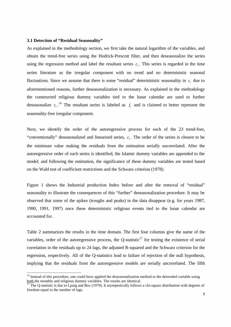
Figure 1 shows the Industrial production Index before and after the removal of “residual”

seasonality to illustrate the consequences of this “further” deseasonalization procedure. It may be

observed that some of the spikes (troughs and peaks) in the data disappear (e.g. for years 1987,

1990, 1991, 1997) once these deterministic religious events tied to the lunar calendar are

accounted for.

Table 2 summarizes the results in the time domain. The first four columns give the name of the

variables, order of the autoregressive process, the Q-statistic17 for testing the existence of serial

correlation in the residuals up to 24 lags, the adjusted R-squared and the Schwarz criterion for the

regression, respectively. All of the Q-statistics lead to failure of rejection of the null hypothesis,

implying that the residuals from the autoregressive models are serially uncorrelated. The fifth

16 Instead of this procedure, one could have applied the deseasonalization method to the detrended variable using both the monthly and religious dummy variables. The results are identical. 17 The Q-statistic is due to Ljung and Box (1979). It asymptotically follows a chi-square distribution with degrees of freedom equal to the number of lags.

10

column gives information about the significance of the religious dummy variables, when they are

included in the “identified” autoregressive regression. A minus sign indicates insignificance of

the coefficients for the religious dummy variables. After all the dummy variables are added to the

regression, the variables with insignificant coefficients are taken out and the test statistics for the

remaining variables are reported. The values of the coefficients as well as the corresponding p-

values for significance are given in the fifth column. As mentioned earlier, if the dummy

variables are significant, it would imply the existence of unaccounted-for seasonality in the data.

Of the 23 variables examined, 8 variables contain significant effects of at least one of the

religious events.18 The next column reports the Wald test statistics19 for testing the joint

significance of the coefficients of the dummy variables of the religious events and the

corresponding p-values. The last two columns report the adjusted R-squared and the Schwarz

criterion associated with the regression including the dummy variables.

Next, we turn to analysis in the frequency domain and estimate the power spectra of tc and tf as

well as the )}%1(100{ α− confidence intervals for all 23 variables. We utilize these to see if the

spectrum of tf improves over the spectrum of tc in terms of Nerlove (1964) and Granger (1978)’s

criterion described earlier, i.e. the adjusted series should not have peaks or dips in the spectrum at

the seasonal frequency and its harmonics.

The estimations are carried out with the Blackman-Tukey Smoothed Periodogram estimator

(1959), discussed in the Appendix. While estimating the power spectrum, we divide the interval

],0[ πω ∈ into 600 frequencies, denoted by j. We compare the spectrum estimates of tc and tf in

the entire range, i.e. 600,...,1=j and pay special attention to the “religious frequency”, the

frequency of a cycle that takes one lunar (Hegirian) year to complete, and its harmonics.20

18 For variables like the industrial production index and its subgroups, the coefficients of the corresponding dummy variables are significantly negative due to the loss of business days. We also observe that the reserve money increases significantly for the months having the two feasts, implying that the open market operations by the central bank provide liquidity to the market during the holidays. These operations are carried out in response to an increase in the liquidity demand prior to the holidays. It is worthwhile to note that Ramadan is significant only one occasion but the feast of Ramadan and feast of Sacrifice have significant effects for almost all 8 variables. 19 The Wald statistic asymptotically follows an F distribution with q,(n-k) degrees of freedom where q is the number of restrictions, n is the sample of variables and k is the number of independent variables in the regression. Equivalently, a chi-square distribution could have also been used. All our results based on the F distribution-based Wald test are also obtained by the chi-square distribution-based Wald test. 20 When a spectrum has a large peak at some frequency ω , then related peaks may occur in the harmonics, i.e. multiples of that frequency. For example if there is a weekly cycle, then there will be bi-weekly, tri-weekly etc. cycles.

11

Therefore, we denote πω 17.0* or 102* ==j 21 and the harmonics of it, i.e.

510408,306,204,=j , the “religious frequencies” in this paper. 22

For each variable, we carry out the following analysis. We first estimate the spectra of tc and tf

along with the confidence bands for those spectra.23 Next, we identify the intervals within the

whole range where the lower bound of a confidence band for the spectrum of tc or tf is strictly

above the upper bound of the confidence band of the spectrum of the other.24 If the lower bound

of the confidence band for the spectrum estimate of tc is strictly above the upper bound of the

confidence band of the spectrum of tf for some frequency band, then we call this “deterioration”.

The opposite case is an “improvement”. If the confidence bands overlap then the two spectra

estimates are not statistically different from each other. This case is noted as “no change”.

Finally, we check if the “religious frequencies” fall into any of the improvement or deterioration

bands for each variable. We only consider bands longer than 12 consecutive frequencies (1% of

the range ]2,0[ πω ∈ ).25

The last two columns of Table 3 summarize these findings. The first of these columns report if an

improvement is observed in the “religious frequencies” and the other column reports the results

for all other frequencies. A variable marked with a plus sign has at least one band marked as

improvement and no bands marked as deterioration. Similarly a variable marked with a minus

sign would have some band marked as deterioration and no bands marked as improvement. A

variable is marked with a plus/minus if for certain frequencies it has improvement and some other

frequencies it has deterioration bands. If the bands for the two spectra intersect for the whole

range, then this is marked with a zero, signifying no change. According to this table we can

classify the variables into 4 categories:

1) Improvement in the whole range and the “religious frequencies”: 2 variables.

21 This corresponds to a cycle of 11.76 months, which is the Hegirian calendar cycle, as it is approximately 353 days. 22 These correspond to cycles of length 5.88, 3.92, 2.94 and 2.35 months or 174, 118, 88, and 70 days. 23 The confidence intervals are 90% confidence intervals. The results are more or less similar when the length of the confidence intervals is set to 95%. 24 We follow this procedure which is “approximate” instead of an “exact” procedure which would involve deriving the distribution of the difference between the spectra of tc and tf and testing the significance of the difference. In Appendix 2 we show that whenever the procedure we follow rejects the hypothesis that the spectra are equal at a given frequency, the “exact” test would reject it as well. 25 As noted in the appendix, the total variance of a series is the sum of the spectra in the range ]2,0[ πω ∈ . So the

above threshold eliminates bands, which correspond to less than 1% of the total variance.

12

2) No change in any frequency: 13 variables.

3) No change in the religious frequencies and deterioration in some other frequencies: 5

variables.

4) Improvement in the religious frequencies and ambiguity, deterioration or no change in the

whole range: 3 variables.

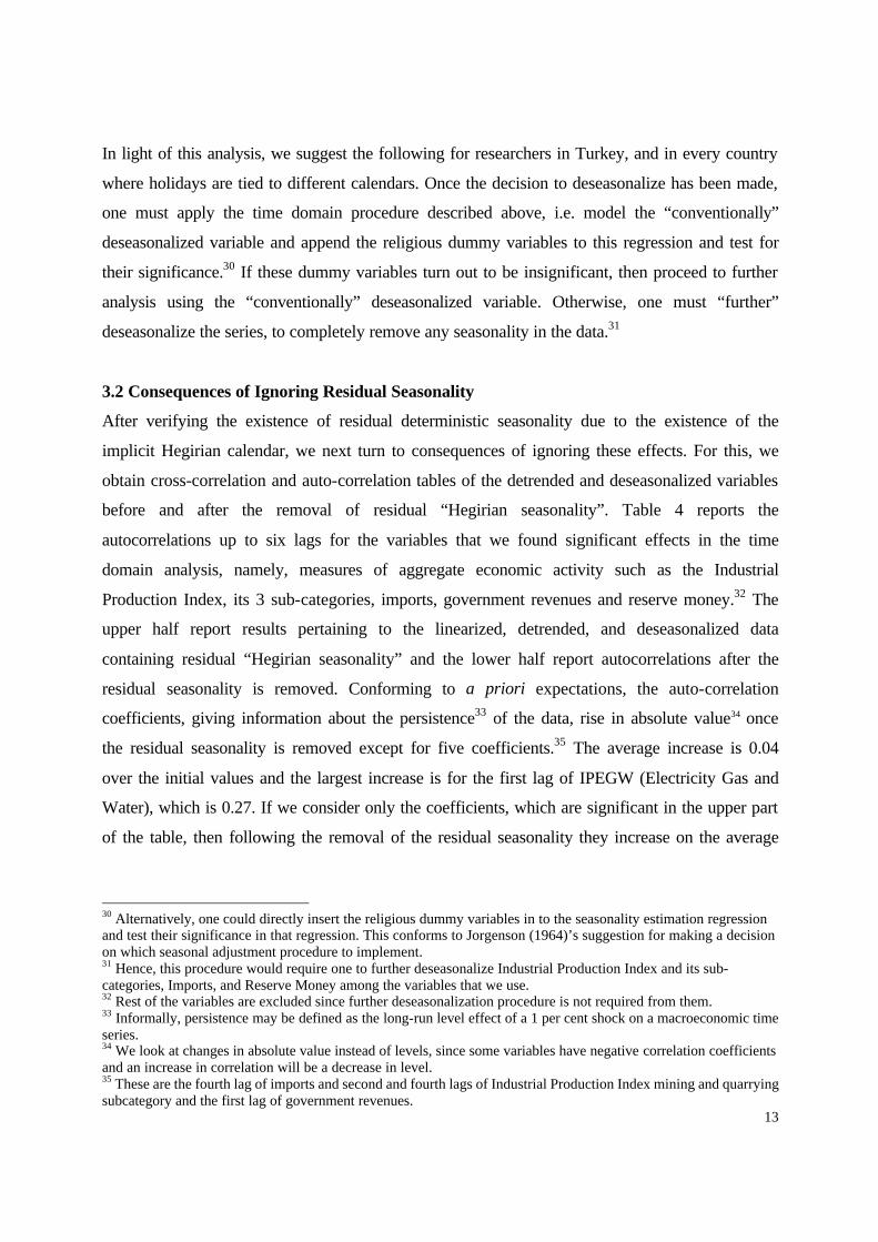
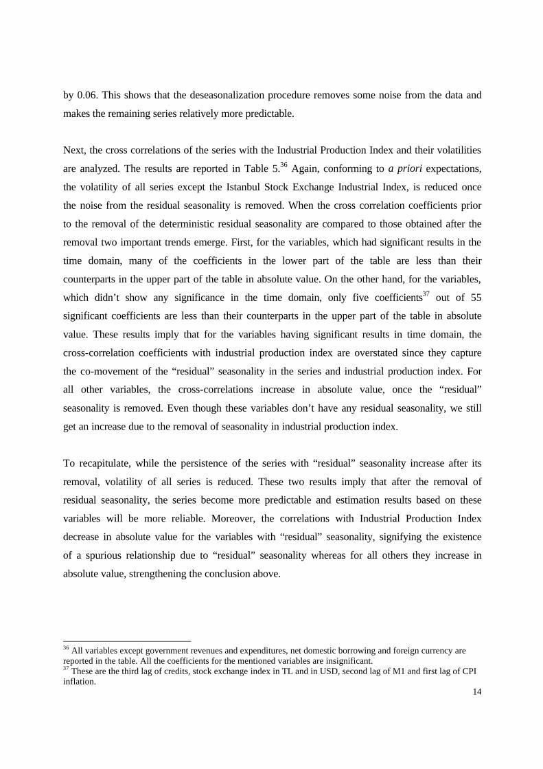
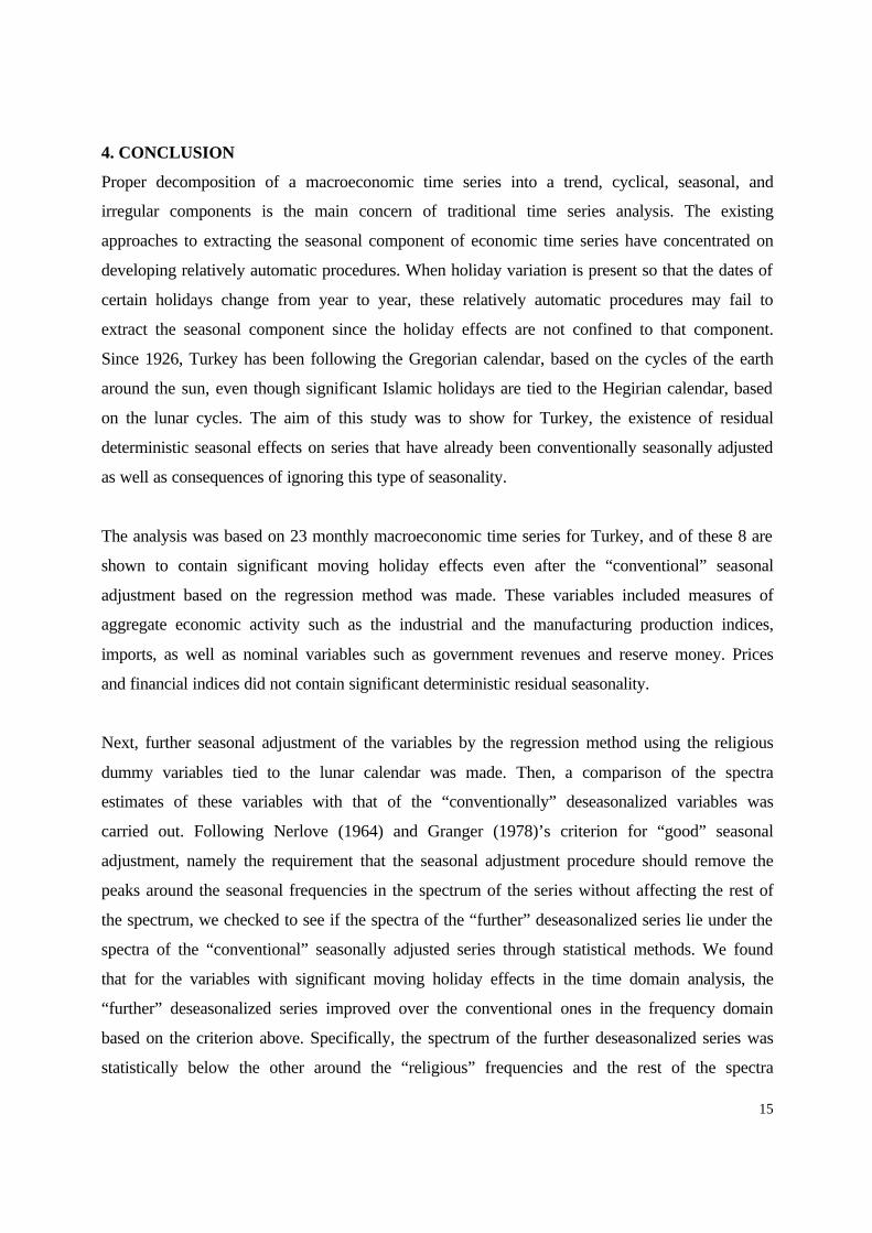
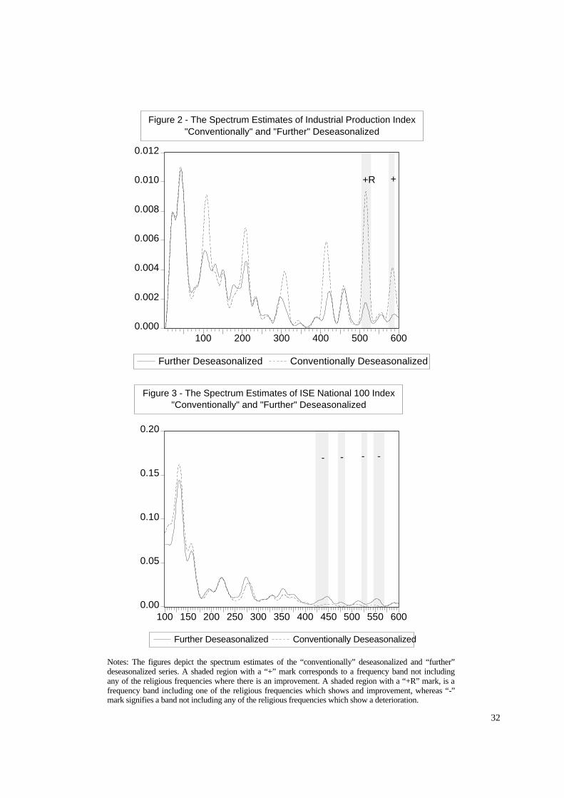
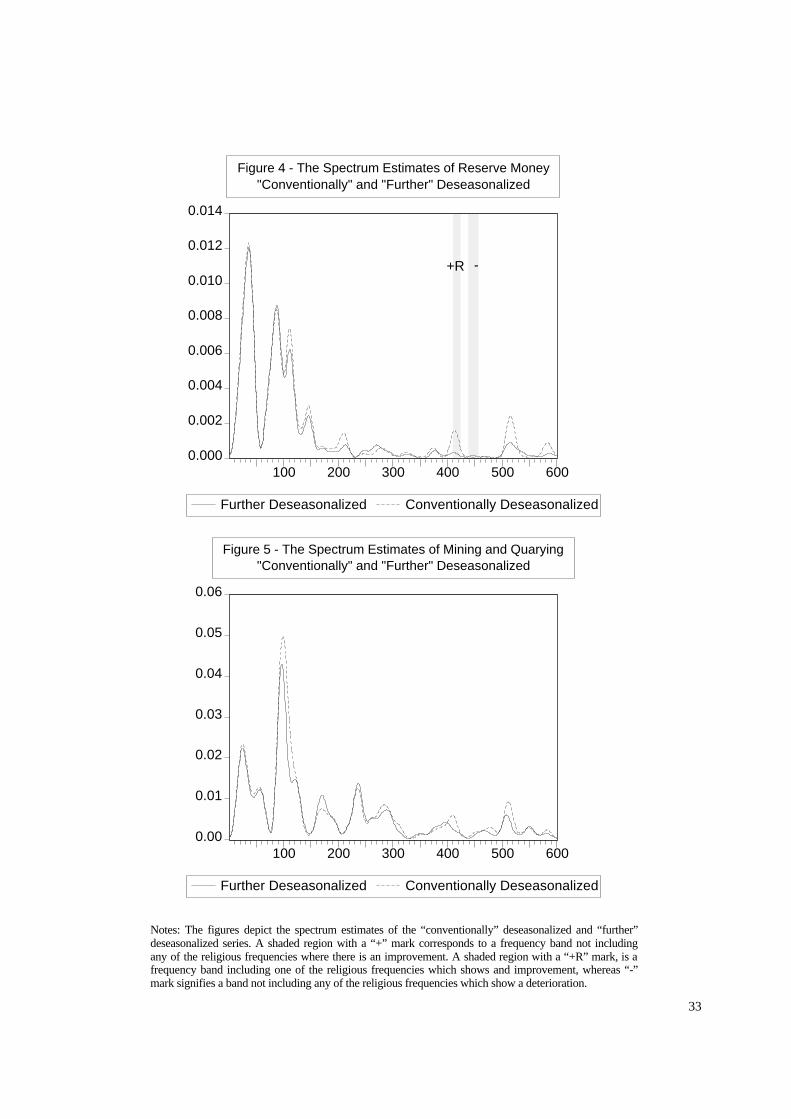
We report the graph for one variable from each category.26 Figures 1 through 4 report the graphs

for Industrial Production Index (Category 1), Mining and Quarrying (Category 2), Istanbul Stock

Exchange National 100 Index (Category 3) and Reserve Money (Category 4). These graphs

include the spectrum estimates for tc and tf with shaded regions. A shaded region with a plus

sign corresponds to a frequency band not including any of the religious frequencies where there is

an improvement. A shaded region with a “+R” mark, is a frequency band including one of the

religious frequencies which shows and improvement, whereas a minus sign signifies a band not

including any of the religious frequencies which show a deterioration.27 All figures except for the

Istanbul Stock Exchange Index in TL depict the spectra for the whole range, for ISETL we start

graphing from j=100 as a peak before that point is very significant and overshadows the

following frequencies.

Table 3 summarizes the main findings. The “significant” / “not significant” entries in the first

column refer to the significance of the Wald test, as given in Table 2.28 The second and third

column summarizes the findings for the frequency domain as described above. The important

result is that if any of the Islamic dummies were significant in the time domain, further

deseasonalization never hurts in the frequency domain, i.e. it gives at least as good results in

terms of Nerlove and Granger’s criterion.29 However, for the variables that the time series

analysis produced an “insignificant” result, i.e. there was no residual seasonality, further

deseasonalization results in either no change or deterioration. This is due to the spurious effects

of the religious dummy variables on the spectrum of the “further” deseasonalized variable.

26 The rest of the graphs are available from the authors. 27 Deterioration at the religious frequencies is not observed for any of the variables. 28 Even though the coefficients for two religious events for CREDIT are individually significant, the joint test of significance gives a p-value of 0.06. Therefore CREDIT will be marked as “not significant”. 29 Only in the case of reserve money, the result is ambiguous.

13

In light of this analysis, we suggest the following for researchers in Turkey, and in every country

where holidays are tied to different calendars. Once the decision to deseasonalize has been made,

one must apply the time domain procedure described above, i.e. model the “conventionally”

deseasonalized variable and append the religious dummy variables to this regression and test for

their significance.30 If these dummy variables turn out to be insignificant, then proceed to further

analysis using the “conventionally” deseasonalized variable. Otherwise, one must “further”

deseasonalize the series, to completely remove any seasonality in the data.31

3.2 Consequences of Ignoring Residual Seasonality

After verifying the existence of residual deterministic seasonality due to the existence of the

implicit Hegirian calendar, we next turn to consequences of ignoring these effects. For this, we

obtain cross-correlation and auto-correlation tables of the detrended and deseasonalized variables

before and after the removal of residual “Hegirian seasonality”. Table 4 reports the

autocorrelations up to six lags for the variables that we found significant effects in the time

domain analysis, namely, measures of aggregate economic activity such as the Industrial

Production Index, its 3 sub-categories, imports, government revenues and reserve money.32 The

upper half report results pertaining to the linearized, detrended, and deseasonalized data

containing residual “Hegirian seasonality” and the lower half report autocorrelations after the

residual seasonality is removed. Conforming to a priori expectations, the auto-correlation

coefficients, giving information about the persistence33 of the data, rise in absolute value34 once

the residual seasonality is removed except for five coefficients.35 The average increase is 0.04

over the initial values and the largest increase is for the first lag of IPEGW (Electricity Gas and

Water), which is 0.27. If we consider only the coefficients, which are significant in the upper part

of the table, then following the removal of the residual seasonality they increase on the average

30 Alternatively, one could directly insert the religious dummy variables in to the seasonality estimation regression and test their significance in that regression. This conforms to Jorgenson (1964)’s suggestion for making a decision on which seasonal adjustment procedure to implement. 31 Hence, this procedure would require one to further deseasonalize Industrial Production Index and its sub-categories, Imports, and Reserve Money among the variables that we use. 32 Rest of the variables are excluded since further deseasonalization procedure is not required from them. 33 Informally, persistence may be defined as the long-run level effect of a 1 per cent shock on a macroeconomic time series. 34 We look at changes in absolute value instead of levels, since some variables have negative correlation coefficients and an increase in correlation will be a decrease in level. 35 These are the fourth lag of imports and second and fourth lags of Industrial Production Index mining and quarrying subcategory and the first lag of government revenues.

14

by 0.06. This shows that the deseasonalization procedure removes some noise from the data and

makes the remaining series relatively more predictable.

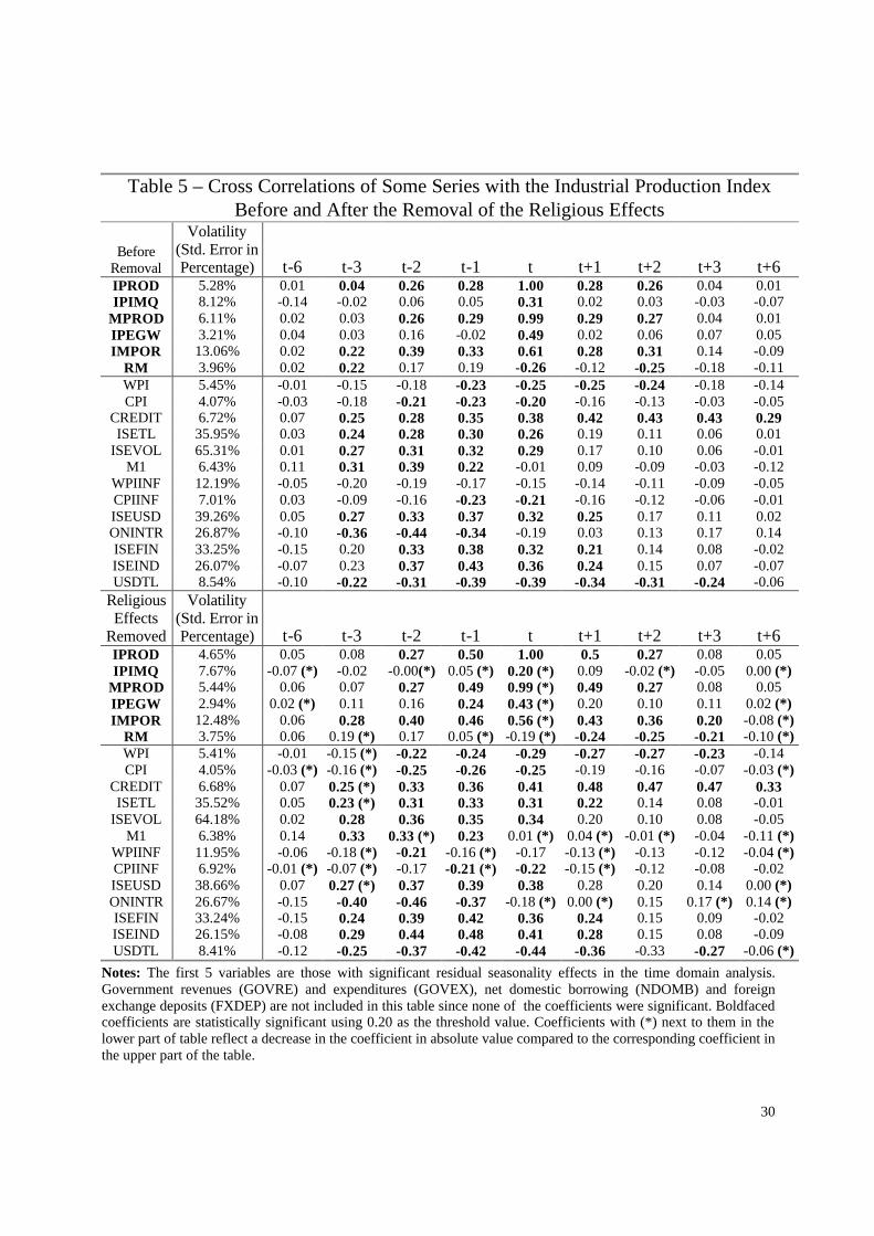
Next, the cross correlations of the series with the Industrial Production Index and their volatilities

are analyzed. The results are reported in Table 5.36 Again, conforming to a priori expectations,

the volatility of all series except the Istanbul Stock Exchange Industrial Index, is reduced once

the noise from the residual seasonality is removed. When the cross correlation coefficients prior

to the removal of the deterministic residual seasonality are compared to those obtained after the

removal two important trends emerge. First, for the variables, which had significant results in the

time domain, many of the coefficients in the lower part of the table are less than their

counterparts in the upper part of the table in absolute value. On the other hand, for the variables,

which didn’t show any significance in the time domain, only five coefficients37 out of 55

significant coefficients are less than their counterparts in the upper part of the table in absolute

value. These results imply that for the variables having significant results in time domain, the

cross-correlation coefficients with industrial production index are overstated since they capture

the co-movement of the “residual” seasonality in the series and industrial production index. For

all other variables, the cross-correlations increase in absolute value, once the “residual”

seasonality is removed. Even though these variables don’t have any residual seasonality, we still

get an increase due to the removal of seasonality in industrial production index.

To recapitulate, while the persistence of the series with “residual” seasonality increase after its

removal, volatility of all series is reduced. These two results imply that after the removal of

residual seasonality, the series become more predictable and estimation results based on these

variables will be more reliable. Moreover, the correlations with Industrial Production Index

decrease in absolute value for the variables with “residual” seasonality, signifying the existence

of a spurious relationship due to “residual” seasonality whereas for all others they increase in

absolute value, strengthening the conclusion above.

36 All variables except government revenues and expenditures, net domestic borrowing and foreign currency are reported in the table. All the coefficients for the mentioned variables are insignificant. 37 These are the third lag of credits, stock exchange index in TL and in USD, second lag of M1 and first lag of CPI inflation.

15

4. CONCLUSION

Proper decomposition of a macroeconomic time series into a trend, cyclical, seasonal, and

irregular components is the main concern of traditional time series analysis. The existing

approaches to extracting the seasonal component of economic time series have concentrated on

developing relatively automatic procedures. When holiday variation is present so that the dates of

certain holidays change from year to year, these relatively automatic procedures may fail to

extract the seasonal component since the holiday effects are not confined to that component.

Since 1926, Turkey has been following the Gregorian calendar, based on the cycles of the earth

around the sun, even though significant Islamic holidays are tied to the Hegirian calendar, based

on the lunar cycles. The aim of this study was to show for Turkey, the existence of residual

deterministic seasonal effects on series that have already been conventionally seasonally adjusted

as well as consequences of ignoring this type of seasonality.

The analysis was based on 23 monthly macroeconomic time series for Turkey, and of these 8 are

shown to contain significant moving holiday effects even after the “conventional” seasonal

adjustment based on the regression method was made. These variables included measures of

aggregate economic activity such as the industrial and the manufacturing production indices,

imports, as well as nominal variables such as government revenues and reserve money. Prices

and financial indices did not contain significant deterministic residual seasonality.

Next, further seasonal adjustment of the variables by the regression method using the religious

dummy variables tied to the lunar calendar was made. Then, a comparison of the spectra

estimates of these variables with that of the “conventionally” deseasonalized variables was

carried out. Following Nerlove (1964) and Granger (1978)’s criterion for “good” seasonal

adjustment, namely the requirement that the seasonal adjustment procedure should remove the

peaks around the seasonal frequencies in the spectrum of the series without affecting the rest of

the spectrum, we checked to see if the spectra of the “further” deseasonalized series lie under the

spectra of the “conventional” seasonally adjusted series through statistical methods. We found

that for the variables with significant moving holiday effects in the time domain analysis, the

“further” deseasonalized series improved over the conventional ones in the frequency domain

based on the criterion above. Specifically, the spectrum of the further deseasonalized series was

statistically below the other around the “religious” frequencies and the rest of the spectra

16

remained statistically unchanged. On the other hand, for variables with insignificant moving

holiday effects in the time domain analysis, further seasonal adjustment did not improve or even

worsened based on the above criterion. The main intuitive conclusion is that one should first

check to see if there exists any “residual” seasonality due to religious effects left in the

“conventionally” deseasonalized series and remove it if it does so. If residual seasonality is not

present, then one should proceed with the conventional adjustment since further adjustment may

not improve the properties of the adjusted series.

Consequences of ignoring the “residual” seasonality were also considered. We calculated the

autocorrelations, volatilities and cross-correlations with output for the variables before and after

the removal of the “residual” seasonality due to moving holidays. We found that the persistence

of the variables containing “residual” seasonality tend to increase with the removal of the

deterministic seasonality tied to the lunar calendar. Moreover, the volatility for almost all

variables decreases after the removal of residual seasonality. These two facts imply that the

variables become relatively more predictable and estimation results based on these variables will

be more reliable when the residual seasonality is removed. When the cross-correlations with

output (industrial production index) were analyzed, we found that the relationship between the

variables that contained residual seasonality is weakened implying the existence of a spurious

relationship caused by common residual seasonality. For all the other variables, on the other

hand, removal of residual seasonality increased the cross-correlations, strengthening our

conclusions for the importance of paying special attention to such residual deterministic

seasonality.

17

APPENDIX 1 : Spectral Density Estimation and Some Important Results

In this section we briefly review some of the important concepts in spectral analysis used in the

paper. 38

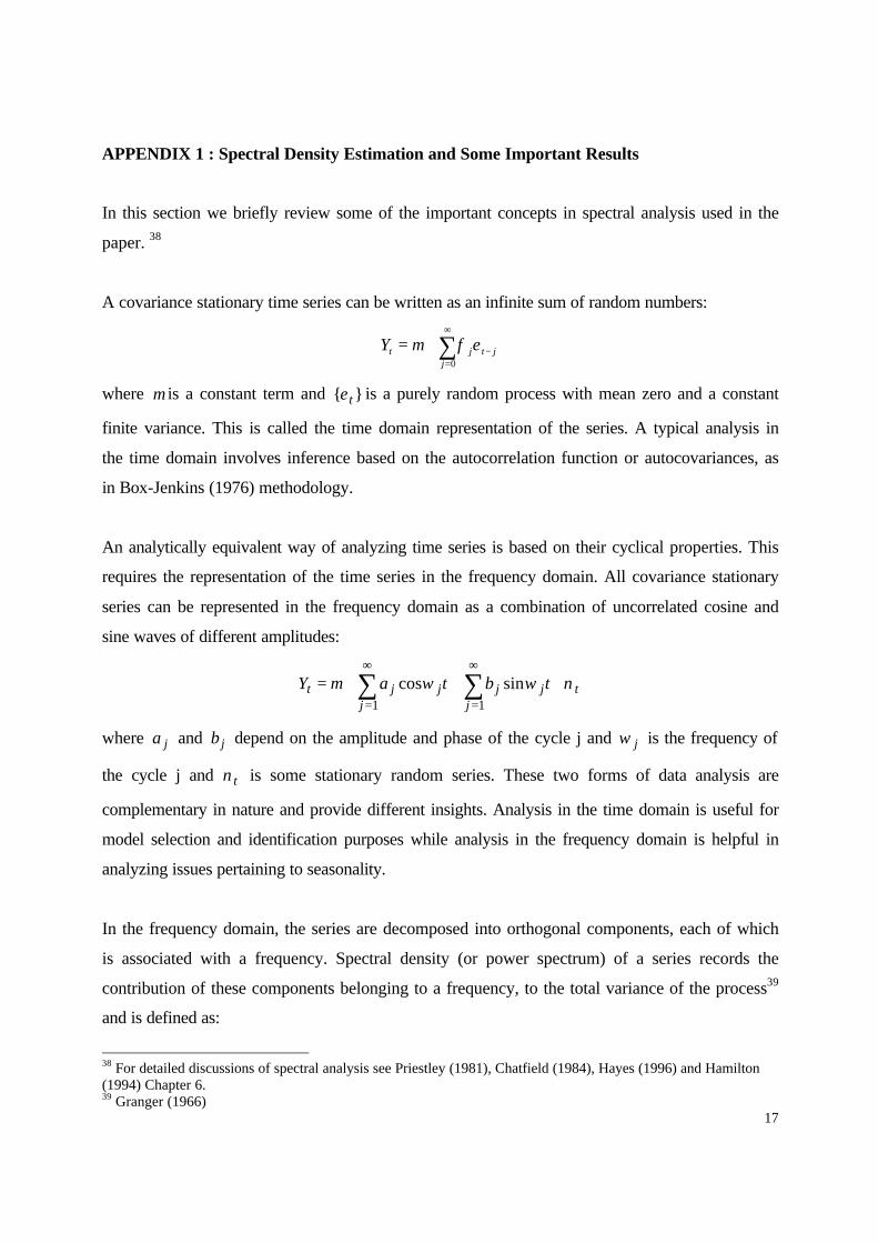
A covariance stationary time series can be written as an infinite sum of random numbers:

∑∞

=−+=

0jjtjtY εφµ

where µ is a constant term and }{ tε is a purely random process with mean zero and a constant

finite variance. This is called the time domain representation of the series. A typical analysis in

the time domain involves inference based on the autocorrelation function or autocovariances, as

in Box-Jenkins (1976) methodology.

An analytically equivalent way of analyzing time series is based on their cyclical properties. This

requires the representation of the time series in the frequency domain. All covariance stationary

series can be represented in the frequency domain as a combination of uncorrelated cosine and

sine waves of different amplitudes:

∑∑∞

=

∞

=

+++=11

sincosj

tjjj

jjt tbtaY νωωµ

where ja and jb depend on the amplitude and phase of the cycle j and jω is the frequency of

the cycle j and tν is some stationary random series. These two forms of data analysis are

complementary in nature and provide different insights. Analysis in the time domain is useful for

model selection and identification purposes while analysis in the frequency domain is helpful in

analyzing issues pertaining to seasonality.

In the frequency domain, the series are decomposed into orthogonal components, each of which

is associated with a frequency. Spectral density (or power spectrum) of a series records the

contribution of these components belonging to a frequency, to the total variance of the process39

and is defined as:

38 For detailed discussions of spectral analysis see Priestley (1981), Chatfield (1984), Hayes (1996) and Hamilton (1994) Chapter 6. 39 Granger (1966)

18

∑∑∞

−∞=

∞

−∞=

− ≤≤−==s

ss

si

s seh πωπωγπ

γπ

ω ω for )cos(2

1

2

1)( 40

where [ ]))(( µµγ −−= −stts YYE is the autocovariance at lag s. As the above definition suggests,

the variance of a series may be obtained by summing the spectra over all frequencies.

The frequency band of interest, by convention, is ],0[ πω ∈ .41 When the plot of the spectrum is

analyzed, a low frequency spike (i.e. higher contribution to total variance of a low frequency) of

the density (small ω , large p) implies a cycle which repeats only a few times in the sample,

whereas a high frequency spike would be a regularity that repeats itself very often.42

The problem at hand is to estimate )(ωh for πω ≤≤0 , given observations ),...,,( 21 TYYY from a

trend-free time series. The obvious choice for this is the periodogram, which is obtained by

replacing the population autocorrelation coefficients by their sample counterparts:

∑−

−−=

−=1

)1(

ˆ21

)(ˆT

Ts

si

sp eh ωγπ

ω

It is documented that the periodogram, although asymptotically unbiased, is an inconsistent

estimator for the population spectrum, since for large s very few observations are used to

compute the autocovariances. 43

For achieving consistency, the Blackman-Tukey (1959) Periodogram Smoothing Method (the

kernel estimate of the spectrum) is used. This method introduces a lag window, )(sλ , that takes

the form

>≤

=M|s| if0

M|s| if)(*)(

ss

λλ

This lag window is a weighting function that puts the largest weights around s=0 and the weights

associated with lags greater than the truncation point, M, are set equal to zero. The reduction of

weights in the tails significantly reduces the variance of the estimator since most of the variance

40 Spectral density is the Fourier transform of the sequence of autocovariances. 41 No information is lost from using this restricted interval. Negative frequencies are not used, because there is no way to decide if the data are generated by a cycle with a frequency ω or ω− . Similarly, any cycle with a frequency greater than π , say πk for 1<k<2, is indistinguishable from a cycle with a frequency π)1( −k . These results follow from trigonometric properties. See Hamilton (1994) p. 160, for details. 42 Granger (1966) argues that a typical economic time series is dominated by low frequency (trend-like) cycles even after detrending.

19

comes from the tail estimates that rely on less number of observations. The Blackman-Tukey

estimate of the spectrum is:

∑−

−−=

=1

)1(

)cos(ˆ)(2

1)(ˆ

T

TssBT ssh ωγλ

πω

Equivalently, )(ˆ ωBTh can be represented as the weighted average of periodogram values of

adjacent frequencies:

θθωωωπ

π

dWhh pBT )()(ˆ)(ˆ −= ∫−

where )(θW is called the spectral window or kernel.44

Under some very mild assumptions about the spectral window, the Blackman-Tukey estimator is

a consistent estimator of the population spectrum at any point. Moreover, as noted by Hayes

(1996), it gives, albeit slightly, better estimates in terms of a criterion based on the normalized

variance.45

It is customary to divide the interval [ ]π,0 into (T-1)/2 frequencies. We will deviate from this

convention and divide the interval into 600 frequencies, given by 600,...,1,1200

2== j

jj

πω . This

doesn’t change the shape, the magnitude of the spectra or the locations of the peaks and troughs

but smoothes out the graph. The relationship between the frequency of a cycle, jω , and the

period of it is j

pj

j12002

==ω

π. This also convenient since, for example, the j=100 frequency

corresponds to one cycle per year, j=200 corresponds to two cycles per year and so on.

43 [ ] [ ]2)()(ˆvar whhp →ω in the limit which is not equal to zero.

44 The lag window is the Fourier transform of the spectral window. ∫−

−−−==π

π

θ θθλ )1(),...,1(for )()( TTsdWes is.

The equivalency of the two representations is obtained by using Fourier transform and convolution theorem. 45 Another consistent estimation method for the spectral density discussed in the literature is the Welch’s Method. (see Welch, 1967 and Hayes, 1996). In this method, the data is divided into K (possibly overlapping) sections and within each section the sample periodograms are averaged using a spectral window. These K numbers are averaged to get an estimate of the spectral density at any point. This method requires less computational power as

20

For carrying out the estimation, one has to choose a lag window and a truncation point. Some

popular lag windows used in the literature are: Bartlett, Tukey-Hamming, Tukey-Hanning,

Blackman.46 For the analysis, Blackman window is used since it shows slightly less variation

compared to other lag windows, which is a desirable property.47 The formula for the Blackman

window is:

>

≤

−−

+

−−

−=M|s| if0

M|s| if1

14cos08.0

1

12cos5.042.0

)( M

s

M

ssB

ππλ

Figure A1 depicts the weight function for Blackman window with M=50. As argued above, the

weight function attaches the highest weight (1) to lag s=0 and the weights decrease for higher

values of s in absolute value. The lags greater than 50 in absolute value are truncated, i.e. given

zero weights.

As for the selection of the truncation point, we follow Jenkins and Watts (1968) and analyze the

spectra using the Blackman window with three different M’s. The smaller the truncation point

(therefore the smaller the bandwidth) the smoother the estimate is. While this reduces variance of

the estimate, the bias increases. Therefore, choosing an intermediate value of M will reduce the

mean square error. We will use M=40 as the truncation point.48 Figure A2 depicts the spectrum

estimates of IPI (detrended and conventionally deseasonalized as explained in the methodology)

with M=10, M=40 and M=75.

autocorrelations are computed for a limited number of observations but its merits are not better than the Blackman-Tukey estimator. 46 See Priestley(1981) for detailed derivations for these windows. 47 Estimates of spectrum using other lag windows produced only slight differences. Moreover, Blackman windows have slightly wider central lobes and less sideband leakage than equivalent length Hamming and Hanning windows. See Oppenheim and Schafer (1989) pp. 447-448 48 The selection of the lag window and truncation point is arbitrary in the literature. However when the same analysis is carried out using different lag windows and truncation points, similar results were obtained. As noted by Priestley

(1981), any αTM = with 10 << α is necessary for consistency of the estimator of the spectral density function.

M=40 corresponds to roughly to 7.0=α .

21

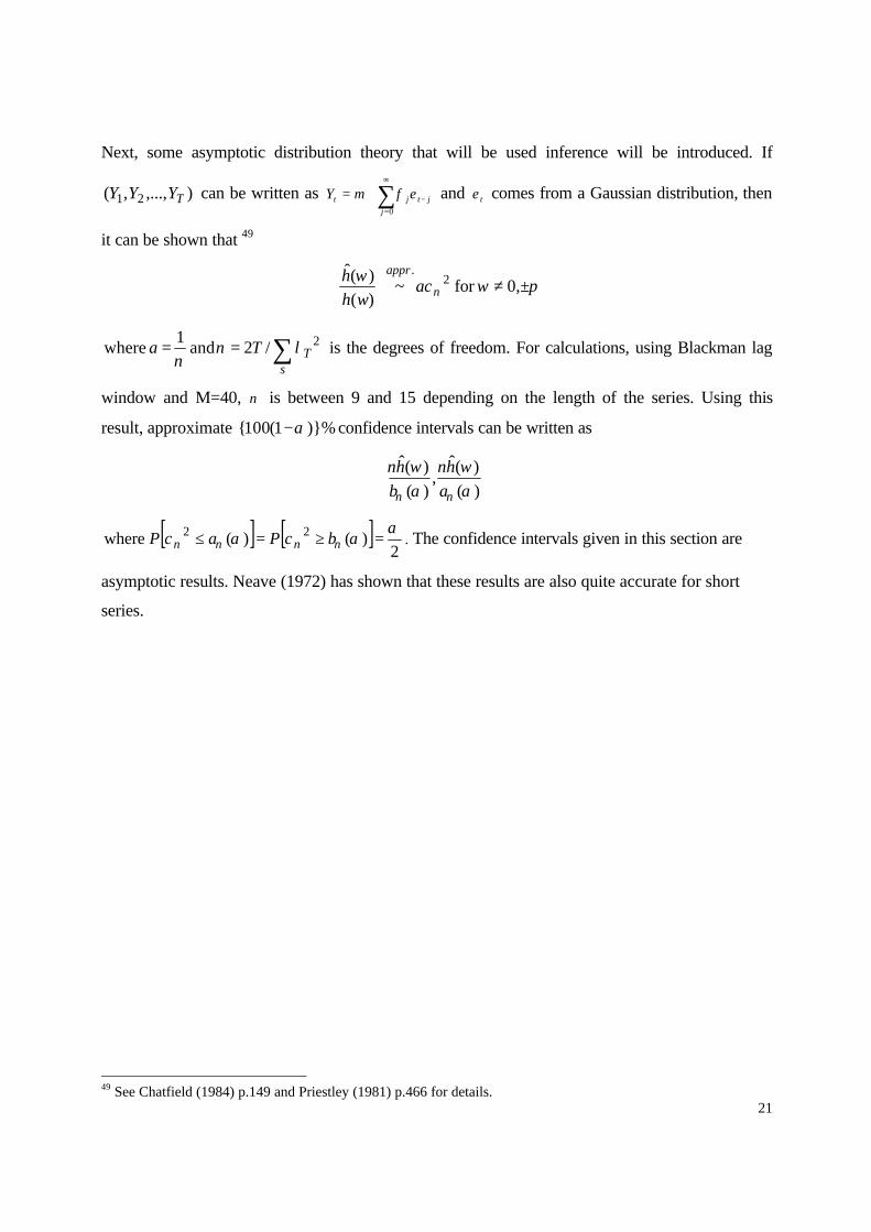
Next, some asymptotic distribution theory that will be used inference will be introduced. If

),...,,( 21 TYYY can be written as ∑∞

=−+=

0j

jtjtY εφµ and tε comes from a Gaussian distribution, then

it can be shown that 49

πωχω

ν ±≠

0,for ~)()(ˆ 2

.a

wh

h appr

/2 and 1

where 2∑==s

TTa λνν

is the degrees of freedom. For calculations, using Blackman lag

window and M=40, ν is between 9 and 15 depending on the length of the series. Using this

result, approximate )}%1(100{ α− confidence intervals can be written as

)(

)(ˆ,

)(

)(ˆ

αων

αων

νν a

h

b

h

[ ] [ ]2

)()( where 22 ααχαχ νννν =≥=≤ bPaP . The confidence intervals given in this section are

asymptotic results. Neave (1972) has shown that these results are also quite accurate for short

series.

49 See Chatfield (1984) p.149 and Priestley (1981) p.466 for details.

22

APPENDIX 2 – Justification of Using Confidence Intervals for Testing The Equality of Two

Spectra at a Given Frequency

In this appendix, we show that whenever the “approximate” procedure we follow in the paper

rejects the hypothesis that two spectra are equal at a given frequency, the “exact” procedure, as

will be made explicit below, rejects it as well.

Consider two estimates )(ˆ ωg and )(ˆ ωh , estimating true spectra )(ωg and )(ωh at the frequencyω .

We want to test

0)()(:

0)()(:0

>−=−

ωωωω

hgH

hgH

A

by using the estimates above, which have the following distributions:

[ ][ ]2

ˆ

2ˆ

),(~)(ˆ

),(~)(ˆ

h

a

g

a

hNh

gNg

σωω

σωω

where 2gσ and 2

hσ are the asymptotic variances of the respective estimates.

The “exact” test, which takes the covariance of )(ˆ ωg and )(ˆ ωh into account50, can be cast in terms

of the confidence interval for the variable )()( ωω hgd −≡ , which is estimated by )(ˆ)(ˆˆ ωω hgd −≡ .

d has the following distribution:

( )hghg

a

Nd ˆˆ

2

ˆ

2

ˆ 2,0~ˆ σσσ −+

The )}%1(100{ α− confidence interval for d is

hghgzd ˆˆ

2

ˆ

2

ˆ2/ 2ˆ σσσα −+±

We would reject 0H in favor of AH if and only if the lower limit of this confidence interval is

greater than 0, i.e.

02ˆˆˆ

2

ˆ

2

ˆ2/ >−+−hghgzd σσσα

In the paper, we use an “approximate” approach in which we conduct our test using the

confidence intervals of )(ωg and )(ωh which are

50 In our case the covariance is very high between the two estimates since one of the series is derived from the other.

23

h

g

zhh

zgg

ˆ2/

ˆ2/

ˆ:)(for Interval Confidence )%1(100

ˆ:)(for Interval Confidence )%1(100

σωα

σωα

α

α

±−

±−

The “approximate” test is conducted as follows: If the lower limit of the confidence interval of

)(ωg is greater than the upper limit of the confidence interval of )(ωh , then the null hypothesis is

rejected in favor of the alternative hypothesis. Thus if

( ) 0ˆˆˆ ˆˆ2/ˆ2/ˆ2/ >+−⇔+>−hghg zdzhzg σσσσ ααα

we conclude that )(ωg is significantly greater than )(ωh at the frequencyω .

Claim: If the lower limit of the confidence interval of )(ωg is greater than the upper limit of the

confidence interval of )(ωh , then the lower limit of the confidence interval of d is greater than 0,

i.e. whenever the “approximate” test rejects 0H in favor of AH , the “exact” test would reject it as

well.

Proof: To prove this claim, it suffices to show that

( )hghghg zdzd ˆˆ2/ˆˆ

2

ˆ

2

ˆ2/ˆ2ˆ σσσσσ αα +−>−+−

or equivalently

hghghg ˆˆ

2

ˆ

2

ˆˆˆ 2σσσσσ −+>+

which would imply that whenever the right hand side is greater than zero, the left hand side also

is. Taking squares of both sides we get

hghghghg ˆˆ

2

ˆ

2

ˆˆˆ

2

ˆ

2

ˆ 22 σσσσσσσ −+>++

hghg ˆˆˆˆ 22 σσσ −>

Using the definition of correlation coefficient hg

hg

hgˆˆ

ˆˆ

ˆˆ σσ

σρ = , we get

1ˆˆ−>

hgρ

which is always true by the definition of the correlation coefficient.

Hence, we show that with underlying normal distributions, using the approximate procedure

gives the same result in terms of rejection of the null hypothesis as the exact test. Since we have

asymptotic results for the spectrum estimates, the above result will be true only asymptotically.

24

References

Alper, C. E. (1998): “Nominal Cycles of the Turkish Business Cycles”, METU Studies in

Development, 25 (2), 1998, pp. 233-244. Alper, C. E. and S. B. Aruoba (2001): “Deseasonalizing Macroeconomic Data: A Caveat to

Applied Researchers in Turkey”, Istanbul Stock Exchange Review, forthcoming. Barsky, R. B. and J. A. Miron (1989): “The Seasonal Cycle and the Business Cycle”, Journal of

Political Economy, 97, No. 3, pp. 503-534. Bell, W. R. and S. C. Hillmer (1983): “Modelling Time Series with Calendar Variation”, Journal

of the American Statistical Association, 78 (253), pp. 526-534. Blackman, R.B. and J. W. Tukey (1959): The Measurement of Power Spectra, Dover, New York. Box, P. and G. Jenkins, (1976): Time Series Analysis, Forecasting and Control, revised ed.,

Holden Day, New York. Chatfield, C. (1984): The Analysis of Time Series: An Introduction, Chapman and Hall, London. Cogley, T. and J. Nason (1995): “Effects of the Hodrick-Prescott Filter on Trend and Difference

Stationary Time Series: Implications for Business Cycle Research”, Journal of Economic Dynamics and Control; 19(1-2), pages 253-78.

Findley, D. F. and R. J. Soukup (2000): “Modeling and Model Selection for Moving Holidays”, 2000 Proceedings of the Business and Economics Statistics Section of the American Statistical Association.

Gersovitz, M. and J. G. MacKinnon (1978): “Seasonality in Regression: An Application of Smoothness Priors”, Journal of the American Statistical Association, 73 (362), pp.264-273.

Granger, C. W. J. (1966): “The Typical Shape of an Economic Variable”, Econometrica, 34 (1), pp. 150-161.

Granger, C. W. J. (1978): “Seasonality: Causation, Interpretation, and Implications”, in Seasonal Analysis of Economics Time Series, Proceedings of the Conference on the Seasonal Analysis of Economic Time Series, Washington DC, 9-10 Sept. 1976 (A. Zellner, ed.), US Department of Commerce, Bureau of the Census, Washington DC.

Grether, D. and M. Nerlove (1970): “Some Properties of ‘Optimal’ Seasonal Adjustment”, Econometrica, 38(5), pp. 682-703.

Hamilton, James D. (1994): Time Series Analysis, Princeton University Press. Hayes, M. H. (1996): Statistical Digital Signal Processing and Modeling, John Wiley & Sons

Inc. Hodrick, R.J. and E.C. Prescott (1997): “Postwar U.S. Business Cycles: An Empirical

Investigation”, Journal of Money, Credit, and Banking; 29(1), pp. 1-16. Hylleberg, S. ed. (1992a): “Modelling Seasonality”, Advanced Texts in Econometrics, Oxford

University Press, New York. Hylleberg, S. (1992b): “The X-11 Method” in Hylleberg, S., ed. Modelling Seasonality,

Advanced Texts in Econometrics, Oxford University Press, New York, pp. 253-57. Jaeger. A. and R. M. Kunst (1990): “Seasonal Adjustment and Measuring Persistence in Output”,

Journal of Applied Econometrics, 5, No. 1, pp. 47-58. Jenkins, G. M. and D. G. Watts (1968): Spectral Analysis and its Applications, Holden-Day, San

Fransisco. Jorgenson, D. W. (1964): “Minimum Variance, Linear, Unbiased, Seasonal Adjustment of

Economic Time Series”, Journal of the American Statistical Association; 59, pp. 681-724. King, R. and S. Rebelo (1993): “Low Frequency Filtering and Real Business Cycles”, Journal of

Economic Dynamics and Control, 17(1-2), pp. 207-31.

25

Lovell, M. C. (1963): “Seasonal Adjustment of Economic Time Series and Multiple Regression Analysis”, Journal of the American Statistical Association; 58, pp. 993-1001.

Ljung, G. and G. Box (1979): “On a Measure of a Lack of Fit in Time Series Models”, Biometrika, 66, pp. 265-270.

Neave, H. R. (1972): “Observations on ‘Spectral Analysis of Short Series – A Simulation Study’ by Granger and Hughes”, Journal of the American Statistical Association, 135, pp. 393-405.

Nerlove, M. (1964): “Spectral Analysis of Seasonal Adjustment Procedures”, Econometrica, 32(3), pp. 241-286

Nerlove, M. (1965): “Comparison of a Modified ‘Hannan’ and the BLS Seasonal Adjustment Filters”, Journal of the American Statistical Association, 60, pp. 442-491.

Oppenheim, A. V. and R. W. Schafer (1989): Discrete-Time Signal Processing” Prentice-Hall. Priestley, M. B. (1981): Spectral Analysis and Time Series – Volume 1 – Univariate Series,

Academic Press. Schwarz, G. (1978): “Estimating the Dimension of a Model”, Annals of Statistics, 6, pp. 461-464. Sims, C. A. (1974): “Seasonality in Regression”, Journal of the American Statistical Association,

69, pp. 618-626. Welch, P.D. (1967) “The Use of Fast Fourier Transform for the Estimation of Power Spectra: A

Method Based on Time Averaging over Short, Modified Periodograms”, IEEE Transactions on Audio and Electroacoustics, AU-15, No.2, pp.70-73.

26

TABLE 1 - Descriptions and Ranges of Variables

Acronym Description Starting Date Ending Date Number of Observations

IPROD SIS Industrial Production Index (1992=100) Jan 1986 April 2000 172

IPIMQ Mining and Quarrying (subgroup of IPROD) Jan 1986 April 2000 172

MPROD Manufacturing Industries (subgroup of IPROD)

Jan 1986 April 2000 172

IPEGW Electricity Gas and Water (subgroup of IPROD)

Jan 1986 April 2000 172

IMPOR Imports (in million USD) Jan 1985 May 2000 185

GOVRE Government Revenues (in million TRL) Jan 1985 June 2000 186

GOVEX Government Expenditures (in million TRL) Jan 1985 June 2000 186

NDOMB Net Domestic Borrowing (in million TRL) Jan 1985 June 2000 186

RM Reserve Money (in million TRL) Sep 1989 Aug 2000 132

M1 M1 (in billion TRL) Jan 1986 April 2000 172

FXDEP Foreign Exchange Denominated Deposit Accounts (in billion TRL)

Jan 1986 April 2000 172

WPI SIS Whole Sale Price Index (1987=100) Jan 1985 June 2000 186

CPI SIS Consumer Price Index (1987=100) Jan 1987 June 2000 162

WPIINF WPI Inflation (year-on-year) Jan 1986 June 2000 174

CPIINF CPI Inflation (year-on-year) Jan 1988 June 2000 150

CREDIT Credits given by Deposit Banks (in billion TRL)

Jan 1986 April 2000 172

ISETL Istanbul Stock Exchange National 100 Index (Monthly Average, TRL Based)

Jan 1986 Aug 2000 176

ISEVOL Istanbul Stock Exchange Trade Volume (Monthly Average)

Nov 1986 Aug 2000 166

ISEUSD Istanbul Stock Exchange National 100 Index (Monthly Average, USD Based)

Jan 1986 Aug 2000 176

ISEFIN Istanbul Stock Exchange Financial Index (Monthly Average, USD Based)

Jan 1991 Aug 2000 116

ISEIND Istanbul Stock Exchange Industrial Index (Monthly Average, USD Based)

Jan 1991 Aug 2000 116

ONINTR Weighted Average of Overnight Simple Interest Rate in Interbank Market

Jan 1990 Aug 2000 128

USDTL Exchange Rate of USD (Central Bank Buying Rate)

Jan 1985 Aug 2000 188

Table 2 – Time Domain Results

Variable Fitted Model

Q-Statistic for 24 lags

Adjusted R-squared and

SC for the Original Model

Religious Events Event / Coefficient / (P-Value)

Wald Test

Statistic

Adjusted R-squared and SC

for the Model with Dummies

IPROD AR(13) 17.47 (0.83)

0.26 -3.21 Feast of Ramadan -0.04 (0.00) Feast of Sacrifice -0.05 (0.00)

11.48 (0.00)

0.35 -3.30

IPIMQ AR(13) 17.87 (0.81) 0.18 -2.43 Feast of Sacrifice -0.04 (0.03)

4.68 (0.03) 0.20 -2.43

MPROD AR(13) 16.71 (0.86)

0.26 -2.95 Feast of Ramadan -0.04 (0.00) Feast of Sacrifice -0.05 (0.00)

10.62 (0.00)

0.35 -3.02

IPEGW AR(13) 17.10 (0.84) 0.09 -4.16 Feast of Ramadan -0.03 (0.00)

Feast of Sacrifice -0.03 (0.00) 16.81 (0.00) 0.25 -4.30

IMPOR AR(11) 20.57 (0.66)

0.51 -1.69 Feast of Ramadan -0.10 (0.00) Feast of Sacrifice -0.07 (0.00)

12.60 (0.00)

0.57 -1.78

GOVRE AR(14) 21.37 (0.62) 0.67 -3.35 Feast of Ramadan -0.02 (0.03) 4.84

(0.03) 0.67 -3.54

GOVEX AR(13) 24.24 (0.45)

0.30 -2.43 - - - -

NDOMB AR(4) 26.88 (0.31)

0.43 0.13 - - - -

RM AR(13) 20.68 (0.66)

0.53 -4.06 Feast of Ramadan 0.02 (0.04) Feast of Sacrifice 0.02 (0.02)

4.22 (0.02)

0.55 -4.06

M1 AR(10) 21.96 (0.58)

0.45 -3.06 -

- - -

FXDEP AR(8) 16.30 (0.88)

0.74 -3.33 - - - -

WPI AR(2) 22.63 (0.54)

0.86 -4.87 - - - -

CPI AR(6) 17.59 (0.82)

0.81 -7.98 - - - -

WPIINF AR(13) 11.25 (0.99)

0.88 -3.15 - - - -

CPIINF AR(10) 24.59 (0.43) 0.83 -4.00 - - - -

CREDIT AR(4) 31.09 (0.15)

0.89 -4.66 Feast of Ramadan 0.02 (0.03) Ramadan -0.05 (0.03)

2.81 (0.06)

0.89 -4.64

ISETL AR(11) 12.96 (0.97) 0.88 -1.01 - - - -

ISEVOL AR(12) 19.10 (0.75)

0.70 1.03 - - - -

ISEUSD AR(11) 9.68 (0.99)

0.89 -0.93 - - - -

ISEFIN AR(11) 9.22

(0.99) 0.80 -0.59 - - - -

ISEIND AR(11) 14.77 (0.93) 0.80 -1.06 - - - -

ONINTR AR(1) 17.52 (0.83)

0.46 -0.42 - - - -

USDTL AR(13) 6.86 (0.99)

0.86 -3.69 - - - -

Notes: Numbers in parentheses below a test statistic is the p-value for that test statistic. For coefficients, the numbers in parentheses are the p-values for the simple t-statistics. In the Religious Events columns, a dash represents no significant effect of religious dummy variables. All t-statistics and the Wald test statistics are significant with 5% significance (except for CREDIT, the Wald test statistic has a p-value of 0.06). All Q-statistics are insignificant, the smallest p-value being 0.15.

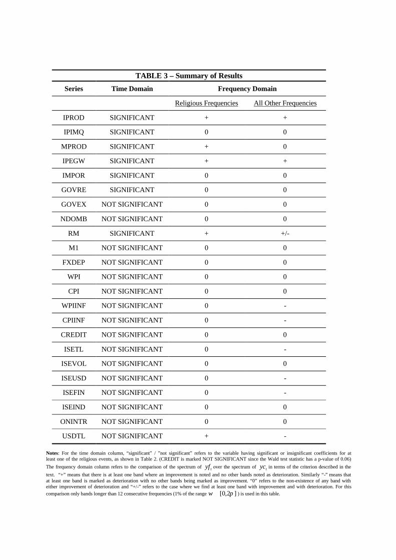
TABLE 3 – Summary of Results

Series Time Domain Frequency Domain

Religious Frequencies All Other Frequencies

IPROD SIGNIFICANT + +

IPIMQ SIGNIFICANT 0 0

MPROD SIGNIFICANT + 0

IPEGW SIGNIFICANT + +

IMPOR SIGNIFICANT 0 0

GOVRE SIGNIFICANT 0 0

GOVEX NOT SIGNIFICANT 0 0

NDOMB NOT SIGNIFICANT 0 0

RM SIGNIFICANT + +/-

M1 NOT SIGNIFICANT 0 0

FXDEP NOT SIGNIFICANT 0 0

WPI NOT SIGNIFICANT 0 0

CPI NOT SIGNIFICANT 0 0

WPIINF NOT SIGNIFICANT 0 -

CPIINF NOT SIGNIFICANT 0 -

CREDIT NOT SIGNIFICANT 0 0

ISETL NOT SIGNIFICANT 0 -

ISEVOL NOT SIGNIFICANT 0 0

ISEUSD NOT SIGNIFICANT 0 -

ISEFIN NOT SIGNIFICANT 0 -

ISEIND NOT SIGNIFICANT 0 0

ONINTR NOT SIGNIFICANT 0 0

USDTL NOT SIGNIFICANT + -

Notes: For the time domain column, “significant” / ”not significant” refers to the variable having significant or insignificant coefficients for at least one of the religious events, as shown in Table 2. (CREDIT is marked NOT SIGNIFICANT since the Wald test statistic has a p-value of 0.06)

The frequency domain column refers to the comparison of the spectrum of tyf over the spectrum of tyc in terms of the criterion described in the

text. “+” means that there is at least one band where an improvement is noted and no other bands noted as deterioration. Similarly “-” means that at least one band is marked as deterioration with no other bands being marked as improvement. “0” refers to the non-existence of any band with either improvement of deterioration and “+/-” refers to the case where we find at least one band with improvement and with deterioration. For this comparison only bands longer than 12 consecutive frequencies (1% of the range ]2,0[ πω ∈ ) is used in this table.

29

Table 4 – Autocorrelations of Chosen Macroeconomic Series Before and After the Removal of the Religious Effects

Before Removal t-6 t-3 t-2 t-1 t t+1 t+2 t+3 t+6 IPROD 0.01 0.04 0.26 0.28 1.00 0.28 0.26 0.04 0.01 IPIMQ -0.24 0.05 0.23 0.48 1.00 0.48 0.23 0.05 -0.24

MPROD 0.02 0.03 0.26 0.31 1.00 0.31 0.26 0.03 0.02 IPEGW -0.10 -0.09 0.11 0.24 1.00 0.24 0.11 -0.09 -0.10 IMPOR 0.06 0.42 0.61 0.56 1.00 0.56 0.61 0.42 0.06 GOVRE 0.38 0.62 0.72 0.82 1.00 0.82 0.72 0.62 0.38

RM -0.13 0.26 0.53 0.68 1.00 0.68 0.53 0.26 -0.13

Religious Effects Removed t-6 t-3 t-2 t-1 t t+1 t+2 t+3 t+6

IPROD 0.05 0.08 0.27 0.49 1.00 0.49 0.27 0.08 0.05 IPIMQ -0.17 (*) 0.08 0.20 (*) 0.50 1.00 0.50 0.20 (*) 0.08 -0.17 (*)

MPROD 0.06 0.06 0.27 0.49 1.00 0.49 0.27 0.06 0.06 IPEGW -0.27 0.01 0.16 0.52 1.00 0.52 0.16 0.01 -0.27 IMPOR 0.07 0.48 0.63 0.66 1.00 0.66 0.63 0.48 0.07 GOVRE 0.38 0.64 0.72 0.82 (*) 1.00 0.82 (*) 0.72 0.64 0.38

RM -0.17 0.30 0.57 0.77 1.00 0.77 0.57 0.30 -0.17

Notes: The variables in this table are those which have significant results in the time domain. Numbers in boldface reflect significant autocorrelation coefficients at 95%. The signicance is determined by threshold values (0.1524 for the first four variables, 0.147 for imports and government revenues and 0.174 for reserve money) which are

calculated using the aymptotic standard error ( )T1 . (*) sign reflects a decrease in the absolute value compared to the value before the religious seasonality is removed.

30

Table 5 – Cross Correlations of Some Series with the Industrial Production Index

Before and After the Removal of the Religious Effects

Before Removal

Volatility (Std. Error in Percentage) t-6 t-3 t-2 t-1 t t+1 t+2 t+3 t+6

IPROD 5.28% 0.01 0.04 0.26 0.28 1.00 0.28 0.26 0.04 0.01 IPIMQ 8.12% -0.14 -0.02 0.06 0.05 0.31 0.02 0.03 -0.03 -0.07

MPROD 6.11% 0.02 0.03 0.26 0.29 0.99 0.29 0.27 0.04 0.01 IPEGW 3.21% 0.04 0.03 0.16 -0.02 0.49 0.02 0.06 0.07 0.05 IMPOR 13.06% 0.02 0.22 0.39 0.33 0.61 0.28 0.31 0.14 -0.09

RM 3.96% 0.02 0.22 0.17 0.19 -0.26 -0.12 -0.25 -0.18 -0.11 WPI 5.45% -0.01 -0.15 -0.18 -0.23 -0.25 -0.25 -0.24 -0.18 -0.14 CPI 4.07% -0.03 -0.18 -0.21 -0.23 -0.20 -0.16 -0.13 -0.03 -0.05

CREDIT 6.72% 0.07 0.25 0.28 0.35 0.38 0.42 0.43 0.43 0.29 ISETL 35.95% 0.03 0.24 0.28 0.30 0.26 0.19 0.11 0.06 0.01

ISEVOL 65.31% 0.01 0.27 0.31 0.32 0.29 0.17 0.10 0.06 -0.01 M1 6.43% 0.11 0.31 0.39 0.22 -0.01 0.09 -0.09 -0.03 -0.12

WPIINF 12.19% -0.05 -0.20 -0.19 -0.17 -0.15 -0.14 -0.11 -0.09 -0.05 CPIINF 7.01% 0.03 -0.09 -0.16 -0.23 -0.21 -0.16 -0.12 -0.06 -0.01 ISEUSD 39.26% 0.05 0.27 0.33 0.37 0.32 0.25 0.17 0.11 0.02 ONINTR 26.87% -0.10 -0.36 -0.44 -0.34 -0.19 0.03 0.13 0.17 0.14 ISEFIN 33.25% -0.15 0.20 0.33 0.38 0.32 0.21 0.14 0.08 -0.02 ISEIND 26.07% -0.07 0.23 0.37 0.43 0.36 0.24 0.15 0.07 -0.07 USDTL 8.54% -0.10 -0.22 -0.31 -0.39 -0.39 -0.34 -0.31 -0.24 -0.06

Religious Effects

Removed

Volatility (Std. Error in Percentage) t-6 t-3 t-2 t-1 t t+1 t+2 t+3 t+6

IPROD 4.65% 0.05 0.08 0.27 0.50 1.00 0.5 0.27 0.08 0.05 IPIMQ 7.67% -0.07 (*) -0.02 -0.00(*) 0.05 (*) 0.20 (*) 0.09 -0.02 (*) -0.05 0.00 (*)

MPROD 5.44% 0.06 0.07 0.27 0.49 0.99 (*) 0.49 0.27 0.08 0.05 IPEGW 2.94% 0.02 (*) 0.11 0.16 0.24 0.43 (*) 0.20 0.10 0.11 0.02 (*) IMPOR 12.48% 0.06 0.28 0.40 0.46 0.56 (*) 0.43 0.36 0.20 -0.08 (*)

RM 3.75% 0.06 0.19 (*) 0.17 0.05 (*) -0.19 (*) -0.24 -0.25 -0.21 -0.10 (*) WPI 5.41% -0.01 -0.15 (*) -0.22 -0.24 -0.29 -0.27 -0.27 -0.23 -0.14 CPI 4.05% -0.03 (*) -0.16 (*) -0.25 -0.26 -0.25 -0.19 -0.16 -0.07 -0.03 (*)

CREDIT 6.68% 0.07 0.25 (*) 0.33 0.36 0.41 0.48 0.47 0.47 0.33 ISETL 35.52% 0.05 0.23 (*) 0.31 0.33 0.31 0.22 0.14 0.08 -0.01

ISEVOL 64.18% 0.02 0.28 0.36 0.35 0.34 0.20 0.10 0.08 -0.05 M1 6.38% 0.14 0.33 0.33 (*) 0.23 0.01 (*) 0.04 (*) -0.01 (*) -0.04 -0.11 (*)

WPIINF 11.95% -0.06 -0.18 (*) -0.21 -0.16 (*) -0.17 -0.13 (*) -0.13 -0.12 -0.04 (*) CPIINF 6.92% -0.01 (*) -0.07 (*) -0.17 -0.21 (*) -0.22 -0.15 (*) -0.12 -0.08 -0.02 ISEUSD 38.66% 0.07 0.27 (*) 0.37 0.39 0.38 0.28 0.20 0.14 0.00 (*) ONINTR 26.67% -0.15 -0.40 -0.46 -0.37 -0.18 (*) 0.00 (*) 0.15 0.17 (*) 0.14 (*) ISEFIN 33.24% -0.15 0.24 0.39 0.42 0.36 0.24 0.15 0.09 -0.02 ISEIND 26.15% -0.08 0.29 0.44 0.48 0.41 0.28 0.15 0.08 -0.09 USDTL 8.41% -0.12 -0.25 -0.37 -0.42 -0.44 -0.36 -0.33 -0.27 -0.06 (*)

Notes: The first 5 variables are those with significant residual seasonality effects in the time domain analysis. Government revenues (GOVRE) and expenditures (GOVEX), net domestic borrowing (NDOMB) and foreign exchange deposits (FXDEP) are not included in this table since none of the coefficients were significant. Boldfaced coefficients are statistically significant using 0.20 as the threshold value. Coefficients with (*) next to them in the lower part of table reflect a decrease in the coefficient in absolute value compared to the corresponding coefficient in the upper part of the table.

31

-0.20

-0.15

-0.10

-0.05

0.00

0.05

0.10

0.15

86 88 90 92 94 96 98 00

REMOVED NOT REMOVED

Figure 1 - Industrial Production IndexBefore and After the Removal of Residual Seasonality

32

0.000

0.002

0.004

0.006

0.008

0.010

0.012

100 200 300 400 500 600

Further Deseasonalized Conventionally Deseasonalized

Figure 2 - The Spectrum Estimates of Industrial Production Index"Conventionally" and "Further" Deseasonalized

+R +

0.00

0.05

0.10

0.15

0.20

100 150 200 250 300 350 400 450 500 550 600

Further Deseasonalized Conventionally Deseasonalized

- ---

Figure 3 - The Spectrum Estimates of ISE National 100 Index"Conventionally" and "Further" Deseasonalized

Notes: The figures depict the spectrum estimates of the “conventionally” deseasonalized and “further” deseasonalized series. A shaded region with a “+” mark corresponds to a frequency band not including any of the religious frequencies where there is an improvement. A shaded region with a “+R” mark, is a frequency band including one of the religious frequencies which shows and improvement, whereas “-” mark signifies a band not including any of the religious frequencies which show a deterioration.

33

0.000

0.002

0.004

0.006

0.008

0.010

0.012

0.014

100 200 300 400 500 600

Further Deseasonalized Conventionally Deseasonalized

Figure 4 - The Spectrum Estimates of Reserve Money"Conventionally" and "Further" Deseasonalized

-+R

0.00

0.01

0.02

0.03

0.04

0.05

0.06

100 200 300 400 500 600

Further Deseasonalized Conventionally Deseasonalized

Figure 5 - The Spectrum Estimates of Mining and Quarying"Conventionally" and "Further" Deseasonalized

Notes: The figures depict the spectrum estimates of the “conventionally” deseasonalized and “further” deseasonalized series. A shaded region with a “+” mark corresponds to a frequency band not including any of the religious frequencies where there is an improvement. A shaded region with a “+R” mark, is a frequency band including one of the religious frequencies which shows and improvement, whereas “-” mark signifies a band not including any of the religious frequencies which show a deterioration.

34

0.0

0.2

0.4

0.6

0.8

1.0

-40 -20 0 20 40

s

Wei

ghts

Figure A1 - Weight Function for Blackman-Tukey Window with M=50

0.000

0.004

0.008

0.012

0.016

100 200 300 400 500 600

M=10 M=40 M=75

j

Figure A2 - Spectrum Estimates of IPI using Blackman-Tukey Method,Blackman Lag Window with M=10,40 and 75