motor control of a hub motor for electric skateboard
TRANSCRIPT

Copyright is owned by the Author of the thesis. Permission is given for a copy to be downloaded by an individual for the purpose of research and private study only. The thesis may not be reproduced elsewhere without the permission of the Author.

i
Motor Control of a Hub Motor for Electric Skateboard Propulsion
A thesis presented in partial fulfilment
of the requirements for the degree of
Masters
in
Engineering
at
Massey University
Palmerston North
New Zealand
Alex Rowe
2016

ii

iii
Abstract An electric powered skateboard was designed and built for testing and development of an innovative hub motor propulsion system and motor controller. The electric skateboard prototype is able to reach speeds of over 50km/h and achieve a range of over 35km on a single battery charge. The prototype weighs 8.6kg and can easily be carried by the user. This mode of transport has potential uses in recreational use, motor sports (racing), short commutes, and most notably, in ‘the last mile’ of public transport – getting to and from a train station, bus stop, etc. to the user’s final destination.
Typical electric powered skateboards use external motors(s) requiring a power transmission assembly to drive the wheels. The hub motor design places the motor(s) inside the skateboard wheels and drives the wheels directly. This removes the need for power transmission assemblies therefore reductions in size, weight, cost, audible noise, and maintenance are realised. The hub motor built for this prototype has proven to be a highly feasible option over typical drive systems and further improvements to the design are discussed in this report.
Advances in the processor capability of low cost microcontrollers has allowed for advanced motor control techniques to be implemented on low cost consumer level motor controllers which, until recent times, have been using the basic ‘Six-Step Control’ technique to drive Permanent Magnet Synchronous Motors. The custom built motor controllers allow for firmware to be flashed to the microcontroller. Firmware was written for the basic motor control technique, Six-Step Control and for the advanced motor control technique, ‘Field Oriented Control’ (FOC). This allowed for the two control techniques to be tested and compared using identical hardware for each.
Six-Step Control drives a three phase motor by controlling the inverter output to six discrete states. The states are stepped through sequentially. This results in a square wave AC waveform. Theory shows that this is not optimal as the magnetic flux produced in the stator is not always perpendicular to the magnet poles but rather aligned to the nearest 60°. FOC addresses this by controlling the magnetic flux to always be perpendicular to the magnet poles in order to maximise torque. The inverter is essentially controlled to produce a continuously variable voltage vector output in terms of both magnitude and direction (vector control).
Bench testing of the control techniques was performed using two motors coupled together with one motor driving and the other motor running as a generator. The generator motor was shown to provide a highly consistent and repeatable load on the driving motor under test and therefore comparisons could be made between the performance of the motor while controlled under Six-Step Control and FOC. This test indicated that FOC was able to drive the motor more efficiently than Six-Step Control, however the FOC implementation requires further development to achieve greater efficiency under high load demands. Furthermore, on-road testing was performed using the motor controllers in the electric skateboard prototype to compare the performance of the two control techniques in a real world application. The results from this test were inconclusive due to large variation in the results between repeated tests.

iv
Acknowledgements In completing this Masters of Engineering degree in Mechatronics, I would like to take this opportunity to sincerely thank:
My Supervisor, Dr Gourab Sen Gupta from the School of Engineering and Advanced Technology (SEAT), Massey University, Palmerston North, New Zealand for his patience and guidance throughout this project.
Mr Clive Bardell and Mr Kerry Griffiths from Massey University’s SEAT workshop and CNC lab for their guidance and expertise in teaching me the skills required to fabricate various parts for the project.
Mr Dennis Rowe, Project Manager at Winstone Pulp International, Karioi, Ohakune, New Zealand for the use of equipment and guidance in building the hub motor prototype.
v
Table of Contents 1. Introduction .................................................................................................................................... 1
1.1. Modern Electric Vehicles ........................................................................................................ 1
1.2. Basic Principles ........................................................................................................................ 2
1.2.1. Batteries .......................................................................................................................... 2
1.2.2. Motor Controller ............................................................................................................. 4
1.2.3. Motor .............................................................................................................................. 6
1.3. Design Objectives .................................................................................................................... 9
2. Basic Principles for Electric Motor Analysis .................................................................................. 10
2.1. Electromagnetic Theory ........................................................................................................ 10
2.1.1. Magnetic Field, B ........................................................................................................... 10
2.1.2. Permeability, μ .............................................................................................................. 10
2.1.3. Magnetic Circuits .......................................................................................................... 11
2.1.4. Magnetic Flux, ФB .......................................................................................................... 12
2.1.5. Flux Linkage, λ ............................................................................................................... 12
2.1.6. Lorentz Force ................................................................................................................ 13
2.1.7. Faraday’s Law of Induction ........................................................................................... 13
2.2. Electric Motor Theory ........................................................................................................... 13
2.2.1. Motor Constant ............................................................................................................. 14
2.2.2. Electric Motor Model .................................................................................................... 16
2.2.3. Saliency ......................................................................................................................... 18
2.2.4. Motor Equations ........................................................................................................... 19
2.2.5. Power Losses ................................................................................................................. 21
2.2.6. Outer Rotor Motor ........................................................................................................ 24
2.3. Motor Control Theory ........................................................................................................... 25
2.3.1. Motor Control Techniques ............................................................................................ 25
2.3.2. Reference Frames ......................................................................................................... 25
2.3.3. Six Step Control ............................................................................................................. 30
2.3.4. Field Oriented Control .................................................................................................. 35
2.3.5. Comparison of Six-Step Control and FOC...................................................................... 38
3. Prototype Design .......................................................................................................................... 39

vi
3.1. Design Considerations ........................................................................................................... 39
3.1.1. Motor Controller ........................................................................................................... 40
3.1.2. Turning Radius .............................................................................................................. 40
3.1.3. Size and Weight ............................................................................................................. 41
3.1.4. Hub Motor Design ......................................................................................................... 41
3.1.5. Physical Layout of Equipment ....................................................................................... 42
3.1.6. Handheld Controller ...................................................................................................... 42
3.2. Power Requirement Modelling ............................................................................................. 43
3.2.1. Model Formulae ............................................................................................................ 43
3.2.2. Matlab Model ................................................................................................................ 47
3.3. Equipment Selection ............................................................................................................. 48
3.3.1. Motors and Wheels ....................................................................................................... 49
3.3.2. Battery Selection ........................................................................................................... 51
3.3.3. Motor Controller ........................................................................................................... 53
3.4. Building the Hub Motor ........................................................................................................ 55
3.4.1. Stator Assembly ............................................................................................................ 55
3.4.2. Rotor Assembly ............................................................................................................. 57
3.4.3. Hall Sensors ................................................................................................................... 58
3.4.4. Temperature Sensors .................................................................................................... 59
3.4.5. Rust Protection ............................................................................................................. 59
3.4.6. Hub Motor Assembly. ................................................................................................... 60
3.5. Electronics Enclosure ............................................................................................................ 61
3.5.1. Equipment Layout ......................................................................................................... 61
3.5.2. Fibreglass Enclosure ...................................................................................................... 61
3.6. Complete Electric Skateboard Prototype .............................................................................. 62
4. Custom Built Motor Controllers .................................................................................................... 63
4.1. Hardware............................................................................................................................... 63
4.1.1. Microcontroller ............................................................................................................. 63
4.1.2. Switching Device ........................................................................................................... 64
4.1.3. Gate Driver .................................................................................................................... 65
4.1.4. Current Sensing ............................................................................................................. 66
4.1.5. Power Supplies .............................................................................................................. 66

vii
4.1.6. DC Bus Capacitors ......................................................................................................... 66
4.1.7. Heat Sink ....................................................................................................................... 69
4.1.8. Hall Sensor Interface ..................................................................................................... 69
4.1.9. Throttle Input ................................................................................................................ 70
4.1.10. Analogue Debug Outputs .............................................................................................. 70
4.1.11. Communication Ports ................................................................................................... 70
4.1.12. Component Layout ........................................................................................................ 71
4.1.13. Complete Motor Controller Hardware ......................................................................... 74
4.2. Software ................................................................................................................................ 74
4.2.1. Six-Step Control ............................................................................................................. 75
4.2.2. FOC ................................................................................................................................ 80
5. Results ........................................................................................................................................... 83
5.1. Bench Testing ........................................................................................................................ 83
5.1.1. Test Rig .......................................................................................................................... 83
5.1.2. Test Setup ..................................................................................................................... 86
5.1.3. Test Results ................................................................................................................... 86
5.1.4. Bench Testing Conclusions ............................................................................................ 89
5.2. On-road Testing .................................................................................................................... 92
5.2.1. Test Rig .......................................................................................................................... 93
5.2.2. Test Setup ..................................................................................................................... 93
5.2.3. Test Results ................................................................................................................... 94
5.2.4. On Road Testing Conclusions ........................................................................................ 99
6. Improvements ............................................................................................................................. 101
6.1. Hub Motor Improvements .................................................................................................. 101
6.1.1. Larger Bearings............................................................................................................ 101
6.1.2. Skateboard Wheel Mechanical Fixing ......................................................................... 101
6.1.3. Custom Wound Stator ................................................................................................ 101
6.2. Motor Controller ................................................................................................................. 102
6.2.1. Miniaturisation ............................................................................................................ 102
6.2.2. Current Sensing Improvements .................................................................................. 102
6.2.3. Fast Over-current Protection ...................................................................................... 102
6.3. General Improvements ....................................................................................................... 103

viii
6.3.1. Battery Isolator ........................................................................................................... 103
6.3.2. Weight Reduction ....................................................................................................... 103
6.3.3. Water Resistance ........................................................................................................ 104
7. Concluding Remarks .................................................................................................................... 105
7.1. Complete Prototype ............................................................................................................ 105
7.2. Hub Motor ........................................................................................................................... 105
7.3. Motor Controller ................................................................................................................. 106
7.4. Motor Control Techniques .................................................................................................. 106
8. References .................................................................................................................................. 108
9. Appendices .................................................................................................................................. 112
Appendix A - Journal Article Published in IEEE International Instrumentation and Measurement Technology Conference (I2MTC 2012) ........................................................................................... 112
Appendix B - Matlab Script for Simulation of the Electric Skateboard Prototype Performance. ... 119
Appendix C - Altium Designer Printouts of the Motor Controller PCB Design ............................... 123
Appendix D- Motor Controller Firmware Source Code................................................................... 134
Appendix E- Bench Testing Minitab Data Analysis ......................................................................... 156
Appendix F - On-road Testing Data Analysis ................................................................................... 180
ix
List of Figures Figure 1.1 - Bar graph showing specific energy densities of common battery chemistries. Lead-acid
batteries are shown in red colour, Nickel based batteries in green, and Lithium based batteries in orange. (Buchmann, 2015) ............................................................................... 3
Figure 1.2 - Three Phase H-Bridge showing flow of current with phase A-High and phase B-Low switches in the ‘on’ state. .................................................................................................... 5
Figure 1.3 - Electric motor classification (Natural Resources Canada, 2014). ........................................ 7
Figure 2.1- Electrical model of the DC motor. ...................................................................................... 16
Figure 2.2- Electrical model of the PMSM. ........................................................................................... 17
Figure 2.3 - Oscilloscope screenshot showing the back EMF waveform of a single phase of the Turnigy C80100 130kv BLDC Motor. .................................................................................. 18
Figure 2.4 - Cross section of an Inner Rotor motor (left) and an Outer Rotor motor (right) illustrating the difference in air-gap radius for the same overall diameter. ....................................... 24
Figure 2.5 - Voltage vector for a three phase PMSM represented in the stator reference frame along with the time varying voltage waveforms. ........................................................................ 27
Figure 2.6 - Voltage vector for a three phase PMSM represented in the alpha-beta reference frame along with the time varying voltage waveforms. .............................................................. 28
Figure 2.7 - Voltage vector for a three phase PMSM represented in the direct-quadrature reference frame along with the time varying voltage waveforms. ................................................... 29
Figure 2.8 - Vector diagram for Six-Step Control showing an arbitrary output vector produced in the second state of the six step sequence. ............................................................................. 31
Figure 2.9 - Timing diagram showing how the Hall sensor output relates to the phase winding back EMF (Microchip Technology Inc., 2003). ........................................................................... 32
Figure 2.10 - Example of a commutation table (Microchip Technology Inc., 2003). ............................ 32
Figure 2.11 - Three phase H-bridge circuit showing current flow for the PWM on period in red, and the freewheeling current during the PWM off period in green. ....................................... 33
Figure 2.12 - Plot of the power dissipated as heat in the semiconductor switch during freewheel current flow through the body diode and the semiconductor switch for the “IRFS7530” transistor. .......................................................................................................................... 34
Figure 2.13 - Block diagram of the FOC technique. .............................................................................. 36
Figure 2.14 - Vector diagram for SVM showing an arbitrary output vector produced in sector ‘S12’ of the SVM scheme. ............................................................................................................... 37
Figure 3.1 - Electric mountain board prototype built as part of final year engineering project. ......... 39
Figure 3.2 - MATLAB Model simulation of the power requirements for the electric longboard as a function of speed and various angles of incline. ............................................................... 47
x
Figure 3.3 - MATLAB model simulation of the range predictions as a function of speed and various angles of incline. ................................................................................................................ 48
Figure 3.4 - MATLAB Model simulation for battery current requirement as a function of speed and various angles of incline. ................................................................................................... 49
Figure 3.5- MATLAB Model simulation for the power loss in each of the two motors as a function of speed and various angles of incline. .................................................................................. 51
Figure 3.6 - MATLAB Model simulation for power loss in the battery pack as a function of speed and various angles of incline. ................................................................................................... 53
Figure 3.7 - MATLAB Model simulation for power loss in each of the two inverters as a function of speed and various angles of incline. .................................................................................. 54
Figure 3.8 - Cross section of the stock Turnigy SK3 6374-149 PMSM. ................................................. 55
Figure 3.9 - The longboard truck after machining, extension of the aluminium axle, and location of the inside end bearing mount. .......................................................................................... 56
Figure 3.10 – Photograph of the modified longboard truck and stator assembly. .............................. 57
Figure 3.11 - Cross section of the motor stator showing the positions of the Hall Effect sensors for 120° electrical spacing. ...................................................................................................... 58
Figure 3.12 - Hall sensor positioned in between stator teeth. ............................................................. 59
Figure 3.13 - Exploded view of the electric longboard hub motor assembly. ...................................... 60
Figure 3.14 - Cross section view of the electric longboard hub motor assembly. ................................ 60
Figure 3.15 - Photograph of the actual electric skateboard hub motor assembly viewed from the underside (left) and the top side (right). ........................................................................... 61
Figure 3.16 - Fibreglass enclosure for the electrical components of the electric longboard. .............. 62
Figure 3.17 – Photograph of the complete electric longboard prototype. .......................................... 62
Figure 4.1 - Snippet from the AUIRFS8409-7P datasheet showing some of the key specifications of the MOSFET that was selected for use in the prototype electric skateboard motor controllers. ........................................................................................................................ 64
Figure 4.2 - Gate drive circuit for a single phase of the custom built motor controller. ...................... 65
Figure 4.3 - Plot illustrating the relationship between ripple current through the bus capacitors and with varying duty cycle for the electric skateboard motor controller. ............................. 67
Figure 4.4 - Plot illustrating the relationship between ripple voltage across the bus capacitors and with varying total bus capacitance for the electric skateboard motor controller. ........... 68
Figure 4.5 - Functional block layout of the Power PCB top side (left) and bottom side (right). ........... 72
Figure 4.6 - Photograph of the assembled power PCB. ........................................................................ 73
Figure 4.7 - Functional block layout of the Control PCB top side (left) and bottom side (right). ......... 73
Figure 4.8 - Photograph of the assembled control PCB top side (left) and bottom side (right). .......... 74
Figure 4.9 - Photograph of the complete motor controller hardware. ................................................ 74
xi
Figure 4.10 - Pin-out graphic generated by "STM32CubeMX" software. ............................................. 78
Figure 4.11 – Clock configuration graphic generated by "STM32CubeMX" software. ......................... 78
Figure 5.1 - Test rig used for the bench testing of the motor controller and the comparison of the two motor control techniques. ......................................................................................... 84
Figure 5.2 - SolidWorks render of the external Hall sensor mounting assembly in exploded view. .... 84
Figure 5.3 – Scatter plot showing the electrical power generated as a function of speed for the four different test scenarios. .................................................................................................... 87
Figure 5.4- Minitab residual plots output for the regression analysis of the combined generator power as a function of speed tests. .................................................................................. 88
Figure 5.5 - Graphical representation of the linear line of best fit models for power input under Six-Step Control and FOC, and power generated as a function of motor speed. ................... 90
Figure 5.6 - Graphical representation of the bench test setup total system efficiency for the driven motor under Six-Step Control and FOC. ............................................................................ 91
Figure 5.7 - Plot showing the difference in total system efficiency for Six-Step Control and FOC as a function of motor speed.................................................................................................... 92
Figure 5.8 - Map showing the route used for the on-road testing. ...................................................... 94
Figure 5.9 - Speed profile for Six-Step Control range and efficiency on-road test number 3 (raw data). ........................................................................................................................................... 95
Figure 5.10 - Speed profile for FOC range and efficiency on-road test number 3 (raw data). ............. 95
Figure 5.11 – Range and efficiency on-road test 3 speed profiles for both Six-Step Control and FOC with inactive periods removed. ......................................................................................... 96
Figure 5.12 - Instantaneous speed measurements for both directions of a single run for Six-Step Control (left) and FOC (right) techniques. ......................................................................... 97
Figure 5.13 - Instantaneous speed measurements for three runs return pass only for Six-Step Control (left) and FOC (right) techniques. ...................................................................................... 97
Figure 5.14 - Instantaneous power measurements for three runs return pass only for Six-Step Control (left) and FOC (right) techniques. ...................................................................................... 98

xii
List of Tables Table 1.1 - Legend for Figure 1.1 ............................................................................................................ 4
Table 3.1 - Comparison of the advantages and disadvantages of a hub motor setup over a reduction drive setup. ........................................................................................................................ 42
Table 3.2 - Electric longboard motor specifications. ............................................................................ 50
Table 3.3 - Electric longboard battery specifications ............................................................................ 52
Table 3.4 - Electric longboard motor controller specifications ............................................................. 54
Table 5.1 - Summary of on-road testing range and efficiency tests for Six-Step Control and FOC techniques. ........................................................................................................................ 96
Table 5.2 - Summary of speed and acceleration data from the three speed test runs for Six-Step Control and FOC techniques. ............................................................................................. 98
Table 5.3 - Summary of power consumption from the three speed test runs for Six-Step Control and FOC techniques. ................................................................................................................. 99

xiii
Glossary Term Definition
Back EMF The voltage that is generated across a motor’s windings as the rotor turns.
Commutation Switching the electrical current path through a motor’s windings in order to achieve continuous rotation.
Copper Loss Power loss in an electric motor associated with the motor’s windings.
Delta (Δ) Refers to three phase loads where the three phases are terminated in a triangle formation.
Eddy current Circulating currents within a conductor due to an induced electromotive force.
Electrical angle The angle of the rotor magnet poles relative to the stator.
H-bridge A transistor arrangement that allows an output to be connected to the positive DC bus or the negative DC bus.
Integrated Development Environment
Refers to a computer programme suite that provides all the necessary tools and resources for programming and developing software.
Iron Loss Power loss in an electric motor associated with the iron core of the electromagnets.
Mains supply A power source from the power supply network. In New Zealand this is 230V, 50Hz single phase AC or 415V, 50Hz three phase AC.
PID Controller An algorithm which aims to regulate an output based on the difference between a set-point and the measured value of the output (error), the sum of previous errors, and the predicted future error.
Rotor The rotating component of an electric motor.
Rotor angle The angle of the rotor relative to the stator.
Remanence The remaining magnetisation of a ferromagnetic material after an external magnet field has been removed.
Stator The stationary component of an electric motor.
Windage loss A term used to represent the energy loss due to the movement of air by a rotating machine.
Wye (Y) Refers to three phase loads where the three phases are terminated in a wye formation. Also commonly referred to as ‘star’ terminated loads.

xiv
Acronyms Term Definition
AC Alternating Current
ADC Analogue to Digital Converter
BLDC Brushless Direct Current
BMS Battery Management System
CAD Computer Aided Design
CNC Computer Numerical Control
DAC Digital to Analogue Converter
DC Direct Current
EMF Electromotive Force
I/O Input / Output
I2C Inter-Integrated Circuit
IC Integrated Circuit
IDE Integrated Development Environment
LEV Light Electric Vehicle
LCD Liquid Crystal Display
MMF Magnetomotive force
PCB Printed Circuit Board
PID Proportional, Integral, Derivative
PM Permanent Magnet
PMSM Permanent Magnet Synchronous Motor
PWM Pulse Width Modulation
RC Radio Controlled
RPM Revolutions per minute
SI Scientific International
SVM Space Vector Modulation
SWD Serial Wire Debug
USART Universal Synchronous Asynchronous Receiver Transmitter

xv
Nomenclature Symbol Definition Units short Units long
A Area m2 Meters squared
B Magnetic field T Tesla
b Friction constant Nm.s/rad Newton meter seconds per radian
C Capacity Ah Amp hours
Cd Coefficient of drag - -
Cr Coefficient of rolling resistance - -
D Wheel diameter m meters
E Electric field N/C Newtons per coulomb
F Force N Newtons
f Frequency Hz Hertz
H Magnetic field Strength A/m
h Time H Hours
I Current A Amperes
J Moment of inertia kg.m2 Kilogram meters squared
km Per phase motor constant Nm/A Newton meters per ampere
Km Total motor constant Nm/A Newton meters per ampere
Kv Motor speed constant V/(rad.s-1) Volts per radians per second
KE Motor eddy current coefficient - -
KH Motor core hysteresis coefficient - -
l Length m Meters
M Multiplier for number of active poles - -
m Mass kg Kilograms
N Number of active turns of wire - -
P Power W Watts
Pe Electrical power W Watts

xvi
Pm Mechanical power W Watts
QH Hysteresis energy loss J/m3 Joules per cubic meter
q Charge C Coulombs
R Resistance Ω Ohms
Rm Reluctance H-1 Inverse henry
r Radius m Meters
t Time s Seconds
V Voltage V Volts
v Velocity m/s Meters per second
vw Wheel Speed km/h Kilometres per hour
ε Electromotive force V Volts
η Efficiency - -
ηd Drive efficiency - -
ηm Motor efficiency - -
θ Angle of incline rad Radians
θm Magnet angle rad radians
ρ Density kg/m3 Kilograms per meter cubed
ρr Resistivity Ωm Ohm meters
τ Torque Nm Newton meters
ω Angular velocity rad/s Radians per second
ФB Magnetic flux Wb Weber
1
1. Introduction
Electric powered vehicles are becoming an increasingly popular and highly viable form of transport, particularly for short distances such as daily commutes to work or school. There are a number of factors driving this expansion; primarily the development of technology used in electric vehicles, making them an attractive option in many cases.
Development of battery technologies, specifically Lithium chemistry batteries, has resulted in batteries being produced that have much higher energy density than previously. The discharge and recharge rates of Lithium chemistry batteries is far superior to other battery chemistries.
Power electronics are becoming more efficient, powerful, and in smaller packages allowing for greater power density in motor controllers with less power loss through the inverter.
Microprocessors with greater processing capacity allow for more efficient motor control algorithms and the use of AC motors instead of DC motors.
With the ever increasing cost fossil fuels – a non-renewable resource that will be depleted in the not so distant future, and advances in technology, electric powered vehicles are becoming an increasingly feasible option.
There are many advantages of using electric motors over internal combustion engines; the running cost is very low, they can achieve near silent operation, and there are no emissions. However there are also limitations; to get the same range as an internal combustion engine driven vehicle, they need large and expensive battery packs. The time it takes to recharge the battery is significantly longer than the time it takes to re-fuel a petrol tank. Therefore journeys that are longer than the range of the battery capacity require a long stop for re-charging.
Given these limitations, this Masters project aims to focus on investigating the gains in performance that can be achieved using advanced motor control techniques, and to apply these to a small electric powered vehicle to compare the performance to that of a typical motor controller.
1.1. Modern Electric Vehicles
Electric vehicles (EVs) have been around since the 1890s but until recent times, have not been a competitive alternative to the Internal Combustion Engine (ICE) due to the price difference and the limited range of the battery powered vehicle. Although the purely electric driven vehicle is mechanically much simpler than the ICE driven vehicle, the energy density of batteries is far lower than that of fossil fuels meaning large and heavy battery packs are required to provide comparable range of the vehicle. This large battery adds significant cost to the EV making it more expensive than a comparable ICE vehicle.
However, the running costs of EVs are much lower than the equivalent ICE vehicle, making modern EVs an attractive alternative. The range shortfall of EVs is becoming less of an issue with high end

2
purely EVs achieving a range of 500km (Tesla Model S). In addition to this, the charge times are significantly reduced with “fast charge” capabilities of 50kW charge power. As an example, a mid-range EV, the Nissan Leaf is able to charge to 80% capacity in 30 minutes and has a range of 170km on a full charge.
As an example, let us compare a low cost ICE driven vehicle to a similar EV. The cost of a new “Toyota Carolla” is $35,000 whereas the cost of the “Nissan Leaf” EV is $60,000 (Lemon & Miller, 2013). The $25,000 difference in cost has a pay-back period of just over 11 years for the average user based on the current electricity and petrol prices (Ecotricity, 2016).
1.2. Basic Principles
This section aims to explain some of the principals that will be used throughout this thesis in order to establish a basis on which more complicated concepts will be explained in the coming sections.
There are three basic components in an electric drive system. A battery, a motor controller, and a motor. The battery supplies energy to the motor controller. The motor controller provides a variable voltage output to the motor in order to control the motor speed or torque. The motor converts electrical energy into kinetic energy in moving the vehicle.
1.2.1. Batteries
A battery is made up of a number of cells connected together in series to achieve the desired voltage. The battery nominal voltage is the single cell nominal voltage multiplied by the number of cells connected in series.
A battery is typically given a capacity rating which is measured in amp hours (Ah) and quantifies the amount of time that the fully charged battery can sustain a load for until it is fully discharged. When comparing the amount of energy a battery can supply in a single charge, the battery voltage must also be taken into account; a 1Ah 3.6V battery cell has three times more energy capacity than that of a 1Ah 1.2V battery cell. Therefore when comparing batteries of different chemistries, the metric watt hours (Wh) is used:
Energy Capacity [Wh] = Current Capacity [Ah] x Voltage [V] (1.1)
Also important in comparing batteries is the discharge rating which specifies what current draw the battery can supply without being damaged. Similarly, the cell voltage should be taken into account to give the power rating. The power rating tells us the rate at which the battery can supply energy in Joules per second (J/s) or Watts (W). The maximum discharge rating is often given in a multiple of the battery’s capacity. For example 20C, which means it is able to supply 20 times the battery capacity. Therefore a 2.2Ah battery rated at 20C discharge has a current rating of 44A.
(1.2)
3
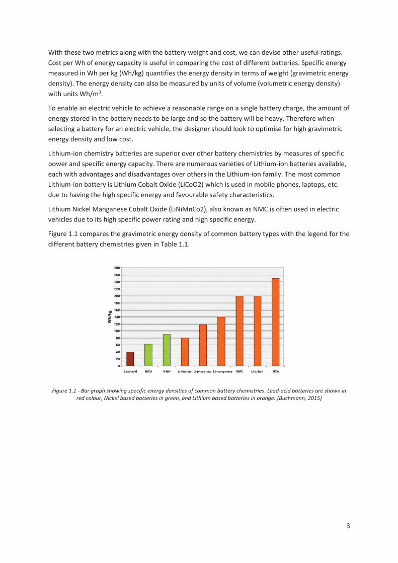
With these two metrics along with the battery weight and cost, we can devise other useful ratings. Cost per Wh of energy capacity is useful in comparing the cost of different batteries. Specific energy measured in Wh per kg (Wh/kg) quantifies the energy density in terms of weight (gravimetric energy density). The energy density can also be measured by units of volume (volumetric energy density) with units Wh/m3.
To enable an electric vehicle to achieve a reasonable range on a single battery charge, the amount of energy stored in the battery needs to be large and so the battery will be heavy. Therefore when selecting a battery for an electric vehicle, the designer should look to optimise for high gravimetric energy density and low cost.
Lithium-ion chemistry batteries are superior over other battery chemistries by measures of specific power and specific energy capacity. There are numerous varieties of Lithium-ion batteries available, each with advantages and disadvantages over others in the Lithium-ion family. The most common Lithium-ion battery is Lithium Cobalt Oxide (LiCoO2) which is used in mobile phones, laptops, etc. due to having the high specific energy and favourable safety characteristics.
Lithium Nickel Manganese Cobalt Oxide (LiNiMnCo2), also known as NMC is often used in electric vehicles due to its high specific power rating and high specific energy.
Figure 1.1 compares the gravimetric energy density of common battery types with the legend for the different battery chemistries given in Table 1.1.
Figure 1.1 - Bar graph showing specific energy densities of common battery chemistries. Lead-acid batteries are shown in
red colour, Nickel based batteries in green, and Lithium based batteries in orange. (Buchmann, 2015)

4
Short Name Long Name Chemical formula
NiCd Nickel Cadmium NiCd
NiMH Nickel Metal Hydride NiMH
Li-titanate Lithium Titanate Li4Ti5O12
Li-phosphate Lithium Iron Phosphate LiFePO4
Li-manganese Lithium Manganese Oxide LiMn2O4
NMC Lithium Nickel Manganese Cobalt Oxide LiNiMnCoO2
Li-cobalt Lithium Cobalt Oxide LiCoO2
NCA Lithium Nickel Cobalt Aluminium Oxide LiNiCoAlO2
Table 1.1 - Legend for Figure 1.1
There are also disadvantages of the Lithium-ion family of batteries. The obvious one being that they cost more than other possible alternatives - Nickel-metal hydride, Nickel-cadmium, and Lead-acid batteries. Lithium-ion batteries can also pose a safety risk if they are not handled properly. Over charging, over discharging, and exceeding the maximum current rating can permanently damage the cells, causing the internal resistance of the battery to increase. This internal resistance creates heat when the battery is charged or discharged. If this heat is great enough the battery can ignite.
To get around this issue, there should be systems in place to prevent the battery from exceeding its ratings. A battery management system (BMS) is often used to monitor the battery and shut off the load if the voltage falls outside of its safe voltage range. A temperature sensor (or sensors) can be incorporated to monitor the battery temperature.
A battery pack is made up of a number of cells connected in series to obtain the desired voltage, and a number of cells connected in parallel to get the desired capacity and current ratings. A convention exists for specifying the battery pack configuration by stating the number of cells connected in series followed by the letter “S”, then the number of cells connected in parallel followed by the letter “P”. For example, a battery pack with “6S2P” configuration specifies that the pack is made up of six cells connected in series, connected in parallel with another string of six cells in series.
Lithium batteries made up with numerous cells connected in series often require ‘balance charging’. This requires a specific charger that is able to charge and discharge individual cells in the battery pack in order to balance the voltage of individual cells rather than just the overall battery voltage. This requires the battery pack to have a balance plug which taps into the individual cells to make them accessible to the charger.
1.2.2. Motor Controller
The purpose of the controller is to control the speed and/or torque output from the motor, based on inputs from the user and other various sensors. It does this by modulating the voltage to the motor, using Pulse Width Modulation (PWM). Most motor controllers used in electric vehicles have some form of current sensing to allow for current limiting or current regulation.

5
1.2.2.1. Pulse Width Modulation
Pulse Width Modulation (PWM) is a technique used to modulate an output by switching an input on and off at some fixed frequency. The ratio of the time that the switch is in the on state to the time that the switch is in the off state is known at the duty cycle. The average output level is directly proportional to the duty cycle. The frequency at which the PWM scheme competes one on and off cycle is known as the switching frequency. The switching frequency should be great enough that there are little or no noticeable pulses, and so PWM simulates an analogue output using a digital (on/off) output.
In the case of a motor controller, the input is the battery voltage which passes through a semiconductor switch to the motor. The average voltage applied to the motor is equal to the battery voltage multiplied by the duty cycle.
Motor controllers use an H-bridge scheme for the switches which allows for current to pass through a motor winding in either direction. In DC motors this allows for reversing the direction of the motor, and in AC motors this is required to make the motor spin continuously.
1.2.2.2. Commutation
In DC motors, commutation is achieved mechanically using a brush and slip ring setup which uses the rotation of the motor to switch the current path between the motor windings in order to get continuous rotation.
AC motors require this commutation to be done externally. A three phase AC motor controller uses three half H-bridges (also called a three phase H-bridge, or three phase inverter) to allow current to flow in either direction through all three phase windings, as illustrated in Figure 1.2 below.
Figure 1.2 - Three Phase H-Bridge showing flow of current with phase A-High and phase B-Low switches in the ‘on’ state.
In this example, the flow of current is shown for the case where ‘Q1’ and ‘Q6’ are in the ‘on’ state. We can see how the flow of current through ‘Phase A’ and ‘Phase B’ could be reversed by simply turning on Q3 and Q4 only.
In its most simple form, a motor controller can drive a 3-phase motor by turning on a pair of switches in the correct sequence. The transition from one step to the next (commutation) must be done at the correct instant to ensure smooth rotation and efficient operation of the motor.

6
1.2.2.3. User Input
A ‘throttle’ input from the user is used to vary the voltage to the motor according to how much throttle input the user is giving. This input is usually used to vary the power to the motor by performing one of the following:
Throttle input is used to directly adjust the PWM duty cycle. Throttle input is used to set a speed reference set-point. The motor controller software uses
a control algorithm (for example, a PID controller) to adjust the PWM duty cycle in order to attempt to achieve an actual motor speed that is the same as the speed reference set-point.
Throttle input is used to set a current reference set-point. The motor controller software uses a control algorithm (for example, a PID controller) to adjust the PWM duty cycle in order to attempt to achieve an actual motor current that is the same as the current reference set-point.
Current regulation provides a more natural feeling throttle response due to the torque produced by the motor being a direct result of the amount of current flowing through the windings. This better simulates a throttle on an internal combustion engine.
1.2.3. Motor
The electric motor is the machine which converts electrical energy to a mechanical torque. Electrical current flowing through the motor windings creates an electromagnetic field which interacts with the ‘rotor’ magnetic field to produce a force on the rotor, causing it to rotate.
There are many different types of electric motors available, each having its own advantages and disadvantages and suitability to a particular application. The different types of motors and applications are vast and therefore this report will not provide an exhaustive discussion on this topic.
Motors can be classified by the type of electrical current they require as an input to make the motor rotate continuously – either AC or DC. Figure 1.3 provides a ‘Family Tree’ for a large number of common electric motor types. Note that the “Universal motor” appears under both AC and DC motor classifications as this motor type runs on either AC or DC electricity.

7
Figure 1.3 - Electric motor classification (Natural Resources Canada, 2014).
Electric Motors
Alternating Current (AC)
Motors
Asychronous
3 phase
Squirrel cage
Wound rotor
Single phase
Permanent split capacitor
Split phase
Capacitor start
Shaded pole
Capacitor run
Variable reluctance
AC Brushed
Universal
Synchronous
Sine wave
Wound rotor
PM rotor
Synchronous condensor
Stepper
Variable reluctance
PM
Hybrid
Brushless
Surface mounted PM
Internal Mounted PM
Reluctance
Synchronous reluctance
Switched reluctance
Direct Current (DC) Motors
Universal
Compound
Shunt
Series

8
1.2.3.1. Stator
The term ‘stator’ refers to the stationary (non-rotating) part of the motor. The stator core is constructed of many thin layers of ‘electrical steel’ (a steel with high silicon content) to create a laminated iron core which the stator windings are looped around to form the coils in an electromagnet.
The stator is constructed in a shape that directs the electromagnetic field outwards in order to maximise the electromagnetic field density at the point where it interacts with the rotor magnetic field to maximise the force exerted on the rotor and hence the torque produced by the motor. There are a number of discrete windings in the stator which are referred to as the stator poles.
1.2.3.2. Rotor
The term ‘rotor’ refers to the rotating part of the electric motor. The rotor produces some form of magnetic field whether it be from a set of permanent magnets, electromagnets, or an induced magnetic. Within a rotor there are a number of discrete magnet field producing devices which are referred to as the rotor poles. The number of magnetic poles will always be an even number; a north and south pole pair is required to produce torque over the full electrical cycle. Pole pairs divide the mechanical rotation of the rotor in to a discrete number of electrical commutation cycles. For example a synchronous motor with 14 magnetic poles has 7 pole pairs and will take 7 electrical commutation cycles to complete one mechanical revolution.
1.2.3.3. AC Motors
AC motors require an Alternating Current (AC) at the motor terminals in order to make the motor rotate continuously. Within this classification there are sub categories for synchronous and asynchronous AC motors.
The AC power source has a cyclical waveform, whether it be a sine or rectangular waveform that repeats at some frequency. This is called the electrical frequency. The actual motor speed (mechanical frequency) may be directly related to the electrical frequency (synchronous motor) or it may run at a mechanical speed that is slower than the synchronous speed (asynchronous motor).
Synchronous motors include Permanent Magnet Synchronous motors (PMSM), separately excited synchronous motors, and switched reluctance motors. These types of motors require that the magnet field produced in the stator must be synchronised with the rotor position in order to optimise the torque output of the motor. In fact, when a synchronous motor loses sync between electrical frequency and mechanical frequency it will likely stall and need to be restarted from zero speed.
Asynchronous motors such as squirrel cage induction motors and wound rotor induction motors require some differential speed between the electrical frequency and mechanical frequency in order to produce torque. The differential speed is referred to as ‘slip speed’ and often expressed as the ratio of differential speed to the synchronous speed.

9
1.2.3.4. DC Motors
A DC motor is one that will rotate continuously when a DC voltage is applied to the motor terminals. A commutator mechanism is used to switch path of the direct current between the discrete windings inside the motor in order to achieve continuous rotation of the rotor. The commutator consists of a ‘brush’ usually constructed of carbon, as a conductor to transfer electrical current to the spinning rotor through the rotor’s ‘slip rings’.
The ‘brushes’ in a DC motor are a consumable part that wears out over time and need to be replaced periodically. The efficiency of the DC motor is also affected from the friction of the brushes against the rotating ‘slip ring’.
However DC motors are still widely used due to the ability to run directly from a battery, and for their simplicity to drive at a variable speed through a DC motor controller, as the controller does not commutate the motor as with an AC motor controller.
1.3. Design Objectives
It was desired to create a prototype EV for this Masters project for the purpose of testing various motor control techniques in a real world application. Obviously it was not practical to create an electric car prototype. Instead the category of Light Electric Vehicles (LEVs) was selected as these are feasible to create on a small budget. The LEV classification applies to land vehicles propelled by an electric motor that uses an energy storage device such as a battery or fuel cell and typically weighs less than 100kg (Benjamin, 2011). The power and energy storage requirements of such vehicles are relatively small and therefore the cost of a LEV is significantly less than an EV.
It was also desired to create a prototype hub motor drive for an electric skateboard application. Therefore a high performance electric skateboard was selected as the basis for the LEV prototype for this Masters project. Some key performance objectives were identified for the electric skateboard, as listed below:
Reach a top speed of 50km/h. Achieve a range of 20km at a speed of 40km/h on an overall level route. To be light enough to comfortably carry – quantified as less than 10kg.
Achieving these objectives would result in a high performance and highly practical LEV for not only recreational use, but also for what some authors call to “the last mile” of travel in public transport. This refers to the gap in where public transport ends and the commuter’s final destination, for example, from a train station to a person’s workplace.

10
2. Basic Principles for Electric Motor Analysis
The previous section gave a brief introduction into electric motors to form a basis on which electric motor theory can be explained. This report will focus on Permanent Magnet Synchronous Motors (PMSM) as this is the motor type that was selected for the prototypes of small electric vehicles by the author, for reasons explained in the following sections.
The PMSM is also commonly referred to as a ‘Permanent Magnet AC Motor’ (PMAC) or a ‘Brushless DC motor’ (BLDC). The term BLDC originates from the concept that the BLDC motor is essentially the same as a Permanent Magnet DC motor without the mechanical commutator (brush and slip ring components). Instead the commutation is done externally using power electronics. However if we define a motor by the type of current that is applied to the motor’s terminals, then the BLDC motor is technically an AC motor. Although the AC electricity applied to a BLDC motor may not be in the form of a sine wave as with other AC motors, the current is still alternating in polarity in order to achieve continuous rotation. Therefore throughout this report, the term PMSM will be used to describe this motor type as it is the technically correct definition.
2.1. Electromagnetic Theory
This section will discuss the physical properties and principals of electromagnetic theory for the purpose of explaining the various aspects of motor control that were investigated in this Masters project. Electromagnet theory forms a basis on which all electric motors operate and motor control techniques relate to the physical operation of a motor.
2.1.1. Magnetic Field, B
The magnetic field denoted by the symbol, ‘B’ describes the strength of a magnetic field. The SI unit for magnetic field is the Tesla (T). Magnetic field is also known as magnetic flux density as the Tesla is equivalent to one webber per square meter (Wb/m2). Magnetic field is sometimes expressed as an ‘H’ field with units amperes per meter. The relationship between B and H Field is determined by the permeability, μ of the material, and calculated by the following equation (Jewett & Serway, 2008).
(2.1)
2.1.2. Permeability, μ
Permeability is a measure of a materials ability to support the formation of a magnetic field within itself. The SI units for permeability is henrys per meter. The permeability of free space, denoted μ0 is

11
a physical constant equal to 4π x 10-7 H/A (Jewett & Serway, 2008). The permeability of specific materials can be obtained from text books or the material datasheet.
Often calculations call for a materials relative permeability to be used. Relative Permeability denoted μr, is defined as the ratio of the material’s permeability to that of free space.
(2.2)
2.1.3. Magnetic Circuits
In a magnetic circuit, the magnetic flux produced by either a permanent magnet or an electromagnet follows a path through various materials from the north pole of the magnet to the south pole. The materials each have a permeability property which effects the total reluctance of the magnetic circuit. The reluctance can be thought of as a resistance to the magnetic flux formation within a material. In the case of an electromagnet, a driving force known as Magnetomotive force creates the force to drive the magnetic flux through the reluctance of the circuit.
2.1.3.1. Magnetomotive Force
Magnetomotive Force (MMF) is the magnetic circuit equivalent of Electromotive Force in an electrical circuit. It quantifies the magnetic force driving a magnetic flux through a magnetic circuit with a magnetic reluctance. The SI unit for MMF is the Ampere-turn. MMF is the product of the current through a coil, I and the number of turns in that coil, N: (Krause, Wasynczuk, Sudhoff, & Pekarek, 2013)
(2.3)
2.1.3.2. Reluctance, Rm
Reluctance of a magnetic circuit is the equivalent of resistance in an electrical circuit. It quantifies how much resistance there is to the magnetic field through a material. The units for reluctance is inverse henry (H-1). Reluctance, Rm is calculated as:
(2.4)
Where l is the length of the material, μ is the permeability, and A is the cross section area. (Krause, Wasynczuk, Sudhoff, & Pekarek, 2013).
Reluctance is also defined in terms of inductance as:
(2.5)
Where N is the number of turns in the coil, L is the inductance of the coil (Krause, Wasynczuk, Sudhoff, & Pekarek, 2013).

12
2.1.3.3. Hopkinson’s Law
Hopkinson’s Law describes a magnetic circuit in analogy to Ohm’s law. Hopkinson’s Law is written as
(2.6)
This expression shows how MMF, magnetic flux, φB and Reluctance, Rm are related (Krause, Wasynczuk, Sudhoff, & Pekarek, 2013).
2.1.4. Magnetic Flux, ФB
Magnetic flux is a measure of the magnetic field which passes through a surface. The SI unit of magnetic flux is the webber (Wb). Magnetic flux, φB is defined as the surface integral of the magnetic field, B with respect to the defined surface, S:
(2.7)
For a uniform magnetic field with a planar surface area, A at an angle, θ to the normal of the field, the magnetic flux is simply expressed as:
(2.8)
In practical terms, a surface is created by a loop of wire and the magnetic flux describes how much magnetic field passes through the area enclosed within the loop of wire.
2.1.5. Flux Linkage, λ
Flux linkage, λ is the total magnetic flux which passes through a coil. The magnetic flux, φB through the surface created by a single loop of wire is replicated for each turn of the N turns within the coil. Flux linkage can simply be written as (Krause, Wasynczuk, Sudhoff, & Pekarek, 2013):
(2.9)
Flux linkage can also be defined as the time integral of the electrical potential (back EMF), ε across the two terminals of the coil (Krause, Wasynczuk, Sudhoff, & Pekarek, 2013):
(2.10)
In differential form, the back EMF produced between the two terminals of the coil is equal to the rate of change in magnetic flux (Krause, Wasynczuk, Sudhoff, & Pekarek, 2013):
(2.11)
13
2.1.6. Lorentz Force
The Lorentz Force law of physics quantifies the force acting on a particle with electrical charge, q moving with a velocity, v in the presence of an electric field, E and magnetic field, B, as shown in the equation below (Jewett & Serway, 2008):
(2.12)
Given the definition of electrical current is the flow of electrical charge in Coulombs per second, and in the absence of an electric field, equation (2.12) becomes:
(2.13)
Equation (2.13) relates the force produced between the stator and rotor of a motor with a given magnet field strength to the amount of current flowing through its winding.
2.1.7. Faraday’s Law of Induction
Faraday’s law of induction quantifies the induced electromotive force (EMF), ε across a conductor by a changing magnetic flux, ФB through a single loop, as shown in the equation below (Jewett & Serway, 2008).
(2.14)
For an electric motor with a discrete number of identical coils of wire, the multiplier, N is added to the equation which represents the number of loops of wire, each with the same magnetic flux through it:
(2.15)
In the case of an electric motor, this equation relates the voltage generated across the motor’s windings to the motion of the rotor. This is referred to as the ‘back EMF’ of the motor and determines how fast the rotor can spin with a given voltage, or how much voltage is generated with a given rotor speed in the case of the electric motor being used as a generator.
2.2. Electric Motor Theory
This section will discuss the physical properties and concepts of an electric motor for the purpose of explaining the various aspects of motor control that were investigated in this Masters project.

14
2.2.1. Motor Constant
The motor constant (km) is among the most important parameters to look for when selecting a motor for a specific application. The motor constant tells us how much torque the motor will produce per ampere of current through it and also how fast it can rotate per volt of electrical potential across the winding.
The motor constant is a characteristic of the motors construction; the number of turns in the stator winding, the length of a single pass of stator wire that is within the magnetic field produced by the permanent magnets (or more conveniently, the length of the magnets), the radius at which force is applied to the rotor (the air gap radius), the strength of the magnets, and the number of stator and magnet poles.
The motor constant can be calculated from the Lorentz Force law by substituting the formula for torque:
(2.16)
Into Equation (2.13) which gives:
(2.17)
Substituting the length of wire as a multiple of the number of turns in each stator pole, and the number of active poles for a single winding, M as a multiplier
(2.18)
Re-arranging gives:
(2.19)
km is defined as the motor constant with units Nm/A:
(2.20)
Substituting km into equation (2.19) gives the equation for the motor constant:
(2.21)
The motor constant has units [Nm/A] and therefore tells us how much torque the motor will produce for a given current. Note that this approach gives the torque constant for a single winding or phase. In a three phase motor with driven from a square wave inverter there are two phases active at a given time. The total torque, Km for this system can be written as:
(2.22)
15
Similarly, a three phase motor driven from a sine wave inverter has total torque, Km given as:
(2.23)
We can also use this figure to calculate the motor speed constant, Kv however we must assume an ideal transformer; the mechanical power output is equal to the electrical power input. This is an assumption that can provide a good ball park figure of the speed constant but for more accurate results the efficiency at a given speed and load must be taken into consideration.
Taking the equation for mechanical power:
(2.24)
And electrical power:
(2.25)
Assuming an ideal transformer:
(2.26)
Substituting equations (2.24) and (2.25) into (2.26):
(2.27)
Re-arranging gives:
(2.28)
Using the definition of the motor speed constant, Kv:
(2.29)
Substituting the definition of km (2.20) and kv (2.29) into equation (2.28):
(2.30)
Therefore the motor constant not only gives an indication of the amount of torque the motor will produce for a given amount of current, but also the speed that the motor is able to spin at for a given voltage. Form this we see that there is a direct trade off between the torque and speed capability of an electric motor. A motor with a large motor constant will produce more torque and spin at a lower speed than that of a small motor constant, given the same voltage and current from the power source.
The speed constant is often converted into more useful units of measure such as volts per RPM (V/RPM) or inverted to give RPM per volt (RPM/V).
16
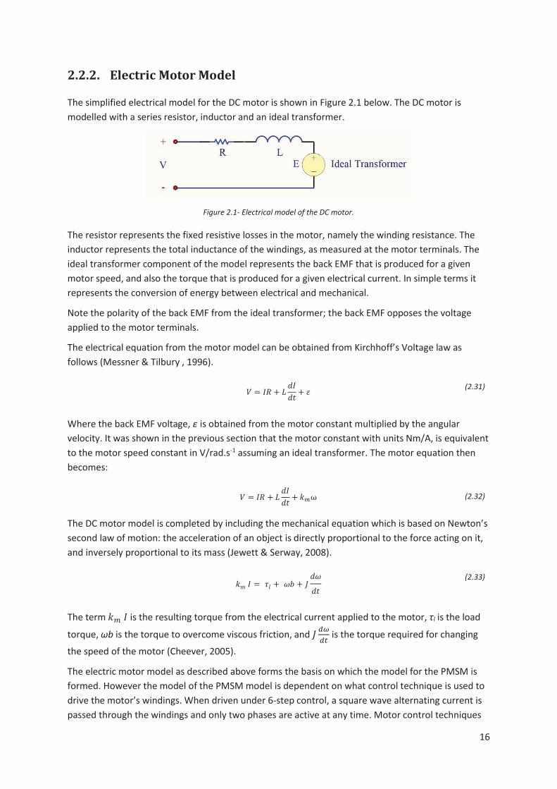
2.2.2. Electric Motor Model
The simplified electrical model for the DC motor is shown in Figure 2.1 below. The DC motor is modelled with a series resistor, inductor and an ideal transformer.
Figure 2.1- Electrical model of the DC motor.
The resistor represents the fixed resistive losses in the motor, namely the winding resistance. The inductor represents the total inductance of the windings, as measured at the motor terminals. The ideal transformer component of the model represents the back EMF that is produced for a given motor speed, and also the torque that is produced for a given electrical current. In simple terms it represents the conversion of energy between electrical and mechanical.
Note the polarity of the back EMF from the ideal transformer; the back EMF opposes the voltage applied to the motor terminals.
The electrical equation from the motor model can be obtained from Kirchhoff’s Voltage law as follows (Messner & Tilbury , 1996).
(2.31)
Where the back EMF voltage, ε is obtained from the motor constant multiplied by the angular velocity. It was shown in the previous section that the motor constant with units Nm/A, is equivalent to the motor speed constant in V/rad.s-1 assuming an ideal transformer. The motor equation then becomes:
(2.32)
The DC motor model is completed by including the mechanical equation which is based on Newton’s second law of motion: the acceleration of an object is directly proportional to the force acting on it, and inversely proportional to its mass (Jewett & Serway, 2008).
(2.33)
The term is the resulting torque from the electrical current applied to the motor, τl is the load
torque, ωb is the torque to overcome viscous friction, and is the torque required for changing the speed of the motor (Cheever, 2005).
The electric motor model as described above forms the basis on which the model for the PMSM is formed. However the model of the PMSM model is dependent on what control technique is used to drive the motor’s windings. When driven under 6-step control, a square wave alternating current is passed through the windings and only two phases are active at any time. Motor control techniques

17
that drive the motor windings using sine wave AC will have all three phases active at a given time, with the voltage magnitude applied to each winding depending on the instantaneous electrical angle. Figure 2.2 shows the model for the three phase PMSM with wye termination.
Figure 2.2- Electrical model of the PMSM.
To describe the three phase AC system, we must introduce the magnet angle, θm which represents the instantaneous position of the rotor’s magnets relative to the stator. Note that the magnet angle is linked to the rotor angle through the number of magnet pole pairs as discussed in section Error! eference source not found..
The three phase motor is constructed with the three phase windings physically distributed evenly around the stator, 120° offset from one phase to the next. The back EMF voltages, ε1, ε2, and ε3 are a function of the magnet angle relative to each phase winding. Setting the magnet angle datum to be aligned with phase number 1, the back EMF voltages can be written as:
(2.34)
(2.35)
(2.36)
This provides a robust model for the three phase system as nothing has been assumed about the shape of the back EMF waveform (Colton, 2008). The actual waveform is cyclic and repeats every full revolution of the magnetic angle. The motor’s construction dictates what the back EMF waveform is. The shape of the permanent magnets, whether the magnets are surface mounted or internal mounted, and the physical distribution of the stator windings play a major role dictating the waveform. It could be trapezoidal or sine wave in shape, or anywhere in between (Mevey, 2006).
The best method of determining the back EMF waveform is experimentally using an oscilloscope. The oscilloscope probe is connected to one of the phase wires and is referenced to the motors ‘neutral’ voltage. A motor with ‘Wye’ connected windings the neutral voltage is the centre of the

18
wye connection. If the motor has ‘delta’ connected windings, or the centre tap of the ‘Wye’ terminated windings is not accessible, the neutral voltage reference can be obtained by centre point re-construction. This is done by connecting the three phases to a common net through a resistor of high resistance in order to simulate the voltage that would be seen at the centre point of the ‘Wye’ terminated winding. Figure 2.3 shows the back EMF waveform from a motor that is marketed as a BLDC motor, the Turnigy C80100 130kv using centre point reconstruction. We can see that this closely resembles a sine waveform.
Figure 2.3 - Oscilloscope screenshot showing the back EMF waveform of a single phase of the Turnigy C80100 130kv BLDC
Motor.
2.2.3. Saliency
To assist in understanding the concept of saliency, consider the magnetic circuit that is observed within an electric motor. An electric current passes through a coil of wire (the winding) producing a magnetic field. The magnetic flux follows a path through various materials within the motor; through the steel core or the stator, across an air gap to the rotor, through the steel in the rotor, back across an air gap, and returning back to the stator steel. Each material in this magnetic circuit has a reluctance to the formation of a magnetic field within itself. The reluctance of ferrous materials such as steel is very small compared to that of the air gap.
Consider a steel rotor which is not cylindrical in cross section. As the rotor turns, the air gap thickness is not constant as observed from a stationary point on the stator. Therefore the reluctance of the magnetic circuit is a function of the rotor angular position. When a coil is energised, the rotor will experience a mechanical torque that will attempt to align the rotor such that the reluctance of the magnetic circuit is minimised.
Electric motors are able to produce mechanical torque by two means; the interaction of magnetic fields or a single magnetic field being driven through a magnetic circuit whose reluctance varies with the rotor angle. The term saliency refers to the latter. For example, a switched reluctance motor has a salient rotor.
A specific motor may be designed to produce torque only through the interaction of magnetic fields, only through a magnetic circuit with reluctance that varies with rotor angle, or a combination of the two.
19
For motors with permanent magnet rotors, the saliency is effected by how the magnets are mounted on the rotor. The magnets themselves have a permeability that is close to that of air.
2.2.3.1. Surface Mounted Magnets
A cylindrical rotor with permanent magnets mounted to the surface or the rotor would be considered a non-salient rotor. Because the magnetic reluctance through the steel in the stator and rotor is very small compared to that of the air gap and permanent magnets, almost all of the MMF is developed across the air gap. As seen from a stationary point on the stator, the reluctance of the magnetic circuit does not vary as the rotor turns. Therefore a non-salient permanent magnet motor is not able to produce torque from the varying reluctance concept.
2.2.3.2. Embedded Magnets
Permanent magnets may be inserted into slots in the rotor. This means that there are gaps in the low reluctance rotor material where the high reluctance permanent magnets are inserted. The result is this is that there is a non-uniform reluctance around the rotor. When observed from a stationary point on the stator, the reluctance of the magnetic circuit varies cyclically as the rotor turns. Therefore a salient PMSM is able to produce torque from the varying reluctance in addition to the interacting magnetic fields of the permanent magnets and stator magnetic fields. This must be allowed for in the control algorithms of such motors.
2.2.4. Motor Equations
As seen previously, modelling the electric motor requires knowledge of the back EMF waveform. In large AC motors, the phase windings are generally distributed such that the back EMF closely resembles a sine wave for the purpose of minimising harmonic distortions in the electrical source. However smaller motors designed for use in electric vehicles are generally designed for maximum power density for the purpose of reducing the size and weight of the motor. Achieving high copper cross section area is given a higher priority than the physical distribution of the windings in order to minimise the phase resistance for a motor which is constrained in size and weight. These motors will typically produce a back EMF waveform that falls somewhere between a sine wave and a trapezoidal wave.
Equation (2.14) states that the back EMF, ε produced across the two terminals of the winding is equal to the rate of change of magnetic flux. The magnetic flux through a winding is a function the instantaneous position of the rotor magnets and the speed at which the rotor is rotating.
The magnetic flux of electromagnetic machines operating in the linear region (not driven into the saturation region) are often expressed in terms of inductances and currents (Krause, Wasynczuk, Sudhoff, & Pekarek, 2013).
Re- arranging equation (2.6) gives:
(2.37)

20
Substituting (2.9) into (2.37):
(2.38)
Substituting (2.3) into (2.38):
(2.39)
Rearranging:
(2.40)
Using the relationship between reluctance and inductance from equation (2.5) we get:
(2.41)
2.2.4.1. Instantaneous Phase Voltage
For a single coil in the presence of a rotating permanent magnet the instantaneous voltage can be written as:
(2.42)
Where:
(2.43)
Rs is the resistance of the coil (stator winding), Is is the current through the winding, λ is the total flux linkage, Lm is the magnetising inductance, Ll is the leakage inductance, λm is the flux linkage from the permanent magnets. Leakage inductance refers to the magnetic flux generated at the end turns of the winding which do not contribute to torque production.
This equation becomes complex when we consider that the variables required in the calculation are not constant; the flux linkage from the permanent magnets are a function of the angular position relative to the stator, θm. The current through the coil is time variant, and the phase inductance is a function of the rotor position relative to the stator. Showing these dependencies, the equation for flux linkage becomes:
(2.44)
Flux linkage from the permanent magnets, λm on the individual three phase windings which are physically distributed at equal spacing around the stator is given as:
(2.45)

21
(2.46)
(2.47)
In a multiphase system we also need to consider the interaction of the flux linkages in the coils for the other phases due to mutual inductance. Reference Krause, Wasynczuk, Sudhoff, & Pekarek, 2013 [pg. 48 – 53] demonstrates the mathematics involved in calculating both self and mutual inductance for the salient and non-salient rotor synchronous motor. It can be proven that mutual inductance, LMutual on one phase from another in a three phase motor is:
(2.48)
It follows that the voltage equations for a single phase, VA of the three phase PMSM can be written as:
(2.49)
(2.50)
Similar equations can be written for the voltage of phase B and C. More conveniently, the three phase system can be expressed in matrix form as follows:
(2.51)
(2.52)
2.2.5. Power Losses
This section will provide an overview of the power losses in an electric drive system for the electric vehicle application. These power losses can be grouped into those occurring in the electric motor and those occurring in the motor controller.
2.2.5.1. Power Loss in the Electric Motor
Mechanical power losses are caused by moving parts. The bearings that support the motor’s rotor have some friction which results in a speed dependent energy loss. Also with increasing motor speed, we have increasing ‘windage loss’ which is the energy loss due to the aerodynamic drag of the rotating machine. These losses can be expressed as a torque load according to the equation
22
(2.53)
Where the first term represents the friction loss and the second term represents the ‘windage loss’. Viscous friction coefficient is given as the symbol b, ω is the angular velocity, Cd is the drag coefficient of the rotor including any cooling fans that may be attached to the rotor, ρ is the fluid density, A is the surface area (The Engineering Toolbox, 2000).
The electrical power loss in an electric motor is often grouped into losses occurring in the motor’s windings, referred to as ‘copper loss’ and losses occurring in the electromagnetic core, referred to as ‘core loss’ or ‘iron loss’.
Copper loss is the loss of energy due to the electrical resistance of a motor’ windings, and is dependent on how much current is flowing.
Iron loss is a combination of energy loss resulting from induced eddy currents in the core material and energy loss due to magnetic remanence (or residual magnetisation) of the core material.
Eddy currents are induced in the core material due to the relative motion of a magnetic field. As stated in Faraday’s law of induction, an electromotive force is created across a conductor by a changing magnetic flux. The core material is conductive, typically constructed of Iron and therefore the induced electromotive force drives an electrical current. This current circulates within the iron core and dissipates energy in the form of heat due to the resistance of the core material.
Eddy currents in an electromagnet generating machine such as the electric motor are minimised by using laminations of the core material, with each lamination electrically isolated from the next. Laminating the core reduces the total loop area of the conductive material within the magnetic field into a large number of small electrically conductive loops. Each small laminate of the core then has an increased electrical resistance and therefore reduces the magnitude of these induced eddy currents (Electrical For You, 2011).
Power loss due to eddy currents can be calculated using the following equation adapted from (Fiorillo, 2004).
(2.54)
Where Peddy is the power loss per unit volume of stator core material, Bp is the peak of the time varying magnetic flux density, l is the lamination thickness, fcom is the frequency at which the magnetic field changes polarity, k is a constant equal to 1 for a sheet conductor, or 2 for a wire conductor, ρr is the resistivity of the core material, D is the density, and m is the mass.
Another form of iron loss is the energy lost due to the remaining magnetisation of the core material, known as remanence. Each time the polarisation of the external magnetic field is reversed, some energy is used in reversing this remaining magnetisation, creating what is known as a hysteresis loss.
This hysteresis loss of the iron core is often approximated using Steinmetz’s equation which gives the energy loss per volume of core material for each cycle of polarity change in the electromagnet, QH. Steinmetz’s equation is given in the following equation (Muhlethaler, Biela, Kolar, & Ecklebe, 2012).
23
(2.55)
Where KH is the hysteresis coefficient which is a property of the core material and can be found experimentally or can be looked up in datasheets, and Bp is the peak of the time varying magnetic flux density. This can be converted to a power loss, Phys by introducing the volume of the core material, Vol, and the frequency at which the polarity is reversed; the commutation frequency fcom.
(2.56)
The core material in electric motors is usually a high silicon content steel, referred to as “Silicon Steel” or “Electrical Steel”. This is a steel that has been designed to possess favourable magnetic properties for use in electromagnets. Specifically, silicon steel has low remanence so that the electromagnetic core has low energy loss due to hysteresis loss, and high permeability so that it is able to produce a high strength magnetic field.
2.2.5.2. Power Loss in the Motor Controller
Power loss in the inverter of the motor controller is a combination of resistive, switching losses, and ‘freewheel’ diode losses in the semiconductor switches. The semiconductor switches have an ‘on-resistance’ given in the device datasheets which is defined as the electrical resistance across the device when the gate conditions are such that the semiconductor is in the fully on state. The power loss due to the on-resistance is simply:
(2.57)
The switching losses are much more complicated in nature however a simplified analysis can be obtained using an idealised approximation for the turn-on and turn-off switching waveforms of the semiconductor switches. Switching loss refers to the power loss in a semiconductor switch which occurs during the transition from the ‘on’ state to the ‘off’ state and vice versa. During this period, the switch has a significant voltage drop across it as well as a significant current flow and therefore a power loss. The formula for this idealised switching loss is: (Markowski, 2002)
(2.58)
Literature shows that this simplified approach to calculating the switching time provides a sufficiently accurate approximation, as demonstrated in (Vishay, 2004).
Additionally, there is another small power loss associated with the switching of the semiconductor devices due to the parasitic capacitance of the transistor, and the charge required to drive the gate. This power loss can be calculated using the formula:
(2.59)
Where Co is the parasitic output capacitance of the transistor, Voff is the voltage across the switch when it is in the off state, fsw is the switching frequency, Qg is the total gate charge, and Vg is the gate drive voltage.

24
Depending on the control scheme, the power loss due to freewheel diode conduction occurs either during the full off state of the PWM cycle, or only during the dead-time inserted for the turn on and turn off transitions when using synchronous switching (refer to section 2.3.3.2).
(2.60)
Where I is the current flow through the transistor, Vf is the forward voltage drop of the diode, tdiode is the time that the diode is conducting during a single PWM cycle, and fsw is the PWM switching frequency. Note that the ‘freewheel’ diode may be a discrete component placed antiparallel to the transistor or it may be the internal ‘body diode’ of the transistor.
2.2.6. Outer Rotor Motor
Traditional motors are constructed with the rotor positioned inside of the stator. It is also possible to reverse this so that the rotor is outside of the stator. Such motors are referred to as Outer Rotor motors. Figure 2.4 illustrates the difference in construction between the traditional Inner Rotor motor and the Outer Rotor motor.
Figure 2.4 - Cross section of an Inner Rotor motor (left) and an Outer Rotor motor (right) illustrating the difference in air-
gap radius for the same overall diameter.
Notice the difference in the radial distance of the permanent magnets and the stator teeth. Because the windings on the stator require a larger width than the magnets, an Outer Rotor motor sees the interaction of magnet fields between the stator and magnets occurring at a greater radius than that of the Inner Rotor motor. This mechanical advantage means that an Outer Rotor motor is able to produce more torque per ampere than the equivalent Inner Runner motor. However there is also a direct trade off in motor speed; an Outer Rotor motor is typically a higher torque and lower speed motor than the an Inner Rotor motor with equivalent size and winding scheme.
Outer Rotor motors form the basis for Hub Motors. A wheel can simply be attached to the outside (rotor) of the motor to create a drive system with no gears, pulleys, or chains required for power transmission.
It should also be noted that the Outer Rotor is a more challenging motor for cooling. A fully closed Outer Rotor motor offers no means of air cooling for the windings. Often this motor type requires

25
openings at each end of the motor to allow air to be forced through the windings. Alternatively liquid coolant may be pumped through channels in the stator as a means of heat removal.
On the other hand, the fully closed Inner Rotor motor sees the stator windings conducting heat to the outer case which may have a fan blowing air over cooling fins as a means of heat removal.
2.3. Motor Control Theory
Motor control theory refers to the various methods of controlling a motor’s speed and/or torque. With many different types of motors available, each with specific control requirements and typically many different methods of control available for each motor type, the field of motor control theory is vast. This thesis will not attempt to summarise the entire field of motor control theory, rather the scope of this thesis will be limited to motor control methods used for the PMSM. PMSMs are widely used in electric vehicle applications ranging from full size passenger cars to small electric vehicles such as electric bikes and skateboards.
2.3.1. Motor Control Techniques
It was decided that this project will focus on comparing the advanced motor control technique, Field Oriented Control (FOC) to the commonly used Six-step motor control technique.
The Six-step control technique has been the control technique of choice for decades in low power, low cost applications such as consumer goods. Examples include household appliances, power tools, RC models, Light Electric Vehicles (LEV) such as electric motorcycles, bikes, scooters, and skateboards. This has been primarily due to the simplicity of the Six-step control algorithm which allows it to be implemented on low cost 8-bit microcontrollers.
In recent times, 32-bit microcontrollers with much higher clock speed and computational capability have become a cost effective alternative. These are beginning to make their way into low cost motor controllers for consumer goods such as those outlined above. With increased computational capability, more advanced motor control techniques are able to be implemented.
This section aims to provide a basic understanding of the two control techniques. To assist in the explanation of how the control techniques work, it is useful to first establish reference frames in which the analysis of the three-phase motor is simplified.
2.3.2. Reference Frames
As demonstrated in section 2.2.4, the motor equations for the three phase PMSM are complex. Some of the machine inductances are functions of rotor speed and therefore the differential equations that describe the behaviour of these machines are time varying (Krause, Wasynczuk, Sudhoff, & Pekarek, 2013). Advanced motor control techniques require such equations to be repeatedly solved at a high rate – often for each period of the PWM cycle which may be in the range of 8 – 20kHz. It is clear that these calculations must be executed in a short amount of time.
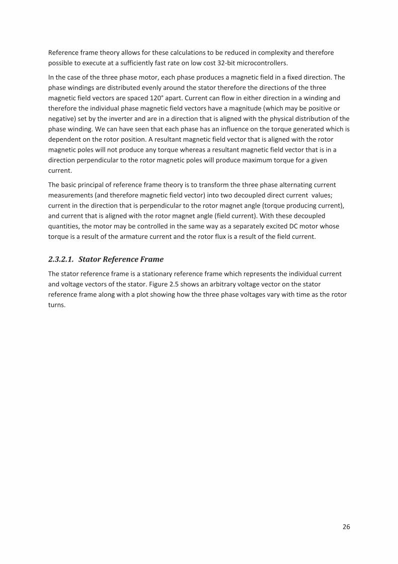
26
Reference frame theory allows for these calculations to be reduced in complexity and therefore possible to execute at a sufficiently fast rate on low cost 32-bit microcontrollers.
In the case of the three phase motor, each phase produces a magnetic field in a fixed direction. The phase windings are distributed evenly around the stator therefore the directions of the three magnetic field vectors are spaced 120° apart. Current can flow in either direction in a winding and therefore the individual phase magnetic field vectors have a magnitude (which may be positive or negative) set by the inverter and are in a direction that is aligned with the physical distribution of the phase winding. We can have seen that each phase has an influence on the torque generated which is dependent on the rotor position. A resultant magnetic field vector that is aligned with the rotor magnetic poles will not produce any torque whereas a resultant magnetic field vector that is in a direction perpendicular to the rotor magnetic poles will produce maximum torque for a given current.
The basic principal of reference frame theory is to transform the three phase alternating current measurements (and therefore magnetic field vector) into two decoupled direct current values; current in the direction that is perpendicular to the rotor magnet angle (torque producing current), and current that is aligned with the rotor magnet angle (field current). With these decoupled quantities, the motor may be controlled in the same way as a separately excited DC motor whose torque is a result of the armature current and the rotor flux is a result of the field current.
2.3.2.1. Stator Reference Frame
The stator reference frame is a stationary reference frame which represents the individual current and voltage vectors of the stator. Figure 2.5 shows an arbitrary voltage vector on the stator reference frame along with a plot showing how the three phase voltages vary with time as the rotor turns.

27
Figure 2.5 - Voltage vector for a three phase PMSM represented in the stator reference frame along with the time varying
voltage waveforms.
2.3.2.2. Alpha-Beta Reference Frame
The Alpha-Beta (α-β) Frame is a stationary reference frame which is obtained by projecting the three phase stator reference frame onto two dimensional orthogonal axis using the ‘Clarke Transformation’. This results in the three stator vectors being reduced to two orthogonal vectors which have the same resultant vector as the original three phase vectors in both direction and magnitude (Krause, Wasynczuk, Sudhoff, & Pekarek, 2013). The Clarke Transformation is a mathematical transformation and is given as:
(2.61)
(2.62)
Transformation from the α-β Frame back to the stator frame is performed using the ‘Inverse Clarke Transformation’ which is:

28
(2.63)
The direction of the alpha and beta axis rotates with the rotor magnet angle as observed from a stationary point on the stator. The angle around the stator which this rotation is referenced to is aligned with phase A.
Taking the same arbitrary voltage as given in Figure 2.5 and imposing it onto the alpha-beta reference frame, we get the three phase voltages represented as two orthogonal values as depicted in Figure 2.6 along with a plot showing how the alpha and beta voltages vary as the rotor turns.
Figure 2.6 - Voltage vector for a three phase PMSM represented in the alpha-beta reference frame along with the time
varying voltage waveforms.
2.3.2.3. Direct-Quadrature Reference Frame
The Direct-Quadrature (d-q) Reference Frame is a two dimensional orthogonal axis frame referenced to a stationary point on the rotor. It is a rotating reference frame which is rotating synchronously
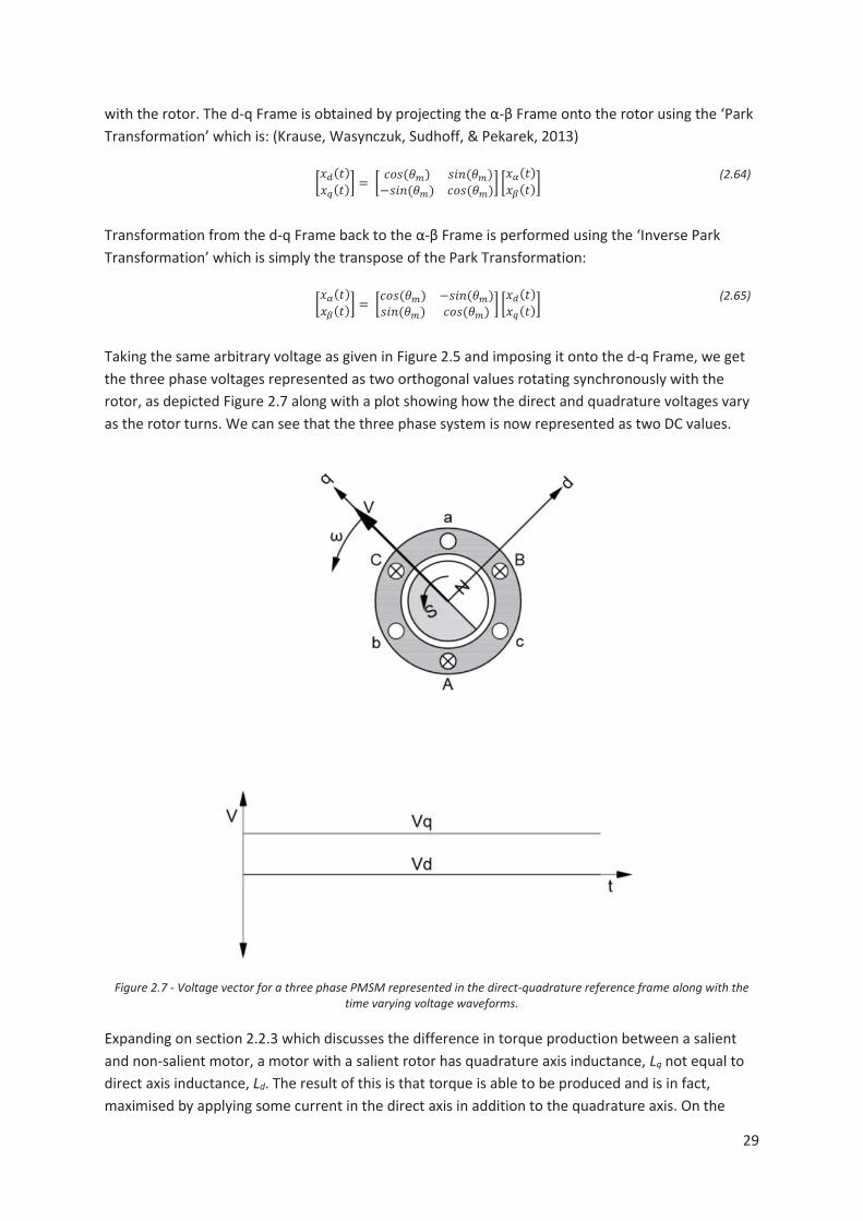
29
with the rotor. The d-q Frame is obtained by projecting the α-β Frame onto the rotor using the ‘Park Transformation’ which is: (Krause, Wasynczuk, Sudhoff, & Pekarek, 2013)
(2.64)
Transformation from the d-q Frame back to the α-β Frame is performed using the ‘Inverse Park Transformation’ which is simply the transpose of the Park Transformation:
(2.65)
Taking the same arbitrary voltage as given in Figure 2.5 and imposing it onto the d-q Frame, we get the three phase voltages represented as two orthogonal values rotating synchronously with the rotor, as depicted Figure 2.7 along with a plot showing how the direct and quadrature voltages vary as the rotor turns. We can see that the three phase system is now represented as two DC values.
Figure 2.7 - Voltage vector for a three phase PMSM represented in the direct-quadrature reference frame along with the
time varying voltage waveforms.
Expanding on section 2.2.3 which discusses the difference in torque production between a salient and non-salient motor, a motor with a salient rotor has quadrature axis inductance, Lq not equal to direct axis inductance, Ld. The result of this is that torque is able to be produced and is in fact, maximised by applying some current in the direct axis in addition to the quadrature axis. On the
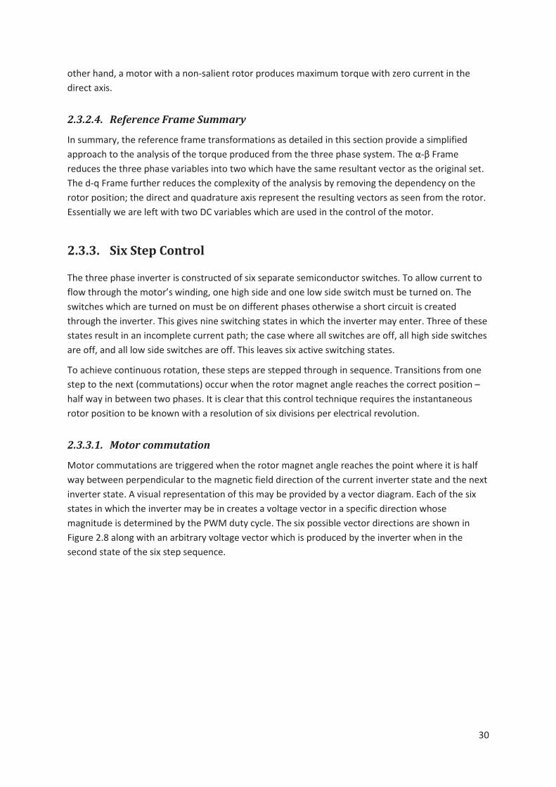
30
other hand, a motor with a non-salient rotor produces maximum torque with zero current in the direct axis.
2.3.2.4. Reference Frame Summary
In summary, the reference frame transformations as detailed in this section provide a simplified approach to the analysis of the torque produced from the three phase system. The α-β Frame reduces the three phase variables into two which have the same resultant vector as the original set. The d-q Frame further reduces the complexity of the analysis by removing the dependency on the rotor position; the direct and quadrature axis represent the resulting vectors as seen from the rotor. Essentially we are left with two DC variables which are used in the control of the motor.
2.3.3. Six Step Control
The three phase inverter is constructed of six separate semiconductor switches. To allow current to flow through the motor’s winding, one high side and one low side switch must be turned on. The switches which are turned on must be on different phases otherwise a short circuit is created through the inverter. This gives nine switching states in which the inverter may enter. Three of these states result in an incomplete current path; the case where all switches are off, all high side switches are off, and all low side switches are off. This leaves six active switching states.
To achieve continuous rotation, these steps are stepped through in sequence. Transitions from one step to the next (commutations) occur when the rotor magnet angle reaches the correct position – half way in between two phases. It is clear that this control technique requires the instantaneous rotor position to be known with a resolution of six divisions per electrical revolution.
2.3.3.1. Motor commutation
Motor commutations are triggered when the rotor magnet angle reaches the point where it is half way between perpendicular to the magnetic field direction of the current inverter state and the next inverter state. A visual representation of this may be provided by a vector diagram. Each of the six states in which the inverter may be in creates a voltage vector in a specific direction whose magnitude is determined by the PWM duty cycle. The six possible vector directions are shown in Figure 2.8 along with an arbitrary voltage vector which is produced by the inverter when in the second state of the six step sequence.
31
Figure 2.8 - Vector diagram for Six-Step Control showing an arbitrary output vector produced in the second state of the six
step sequence.
Some form of rotor position sensing is required to create these commutation triggers. Often dedicated sensors are installed in the motor for rotor position sensing. Motor controllers that require external rotor position sensors are referred to as ‘sensored’ motor controllers. Alternatively the rotor position sensing may be done indirectly without the need for dedicated position sensors in the motor. These motor controllers are referred to as ‘sensorless’ motor controllers.
Sensored Rotor Position Feedback
A sensored motor controller requires inputs from an external sensor or sensors to determine which inverter state is required in order to make the rotor continue to rotate. ‘Hall effect’ sensors are often used for this purpose. The Hall Effect sensors work on the principal that a current carrying plate in the presence of an external magnetic field experiences a voltage differential from one side of the plate to the other. The sensors are typically installed inside the motor on the stator so that the permanent magnets on the rotor trigger the hall sensors output.
There are a number of different types of Hall Effect sensors available. For the purpose of motor control rotor position sensing, digital output, bipolar, latching Hall Effect sensors are used. Three of these sensors are positioned directly facing the permanent magnets and are spaced evenly at 120° (electrical) around the stator. These sensors trigger when commutations occur and therefore it is important to position the sensors correctly relative to the corresponding phase windings. The three output signals from the hall sensors then resemble the waveform as depicted in Figure 2.9.

32
Figure 2.9 - Timing diagram showing how the Hall sensor output relates to the phase winding back EMF (Microchip
Technology Inc., 2003).
The correct inverter state in order to make the motor continue to spin is determined directly from reading the hall sensor inputs. A commutation table may be written which the motor controller uses to determine which switches to turn on. The following table is an example from reference: Microchip Technology Inc., 2003. A similar table may be written for running the motor in the reverse direction.
Figure 2.10 - Example of a commutation table (Microchip Technology Inc., 2003).
Sensorless Rotor Position Feedback
Alternatively, the instantaneous rotor position may be determined by indirect means in ‘sensorless’ operation. This can be done by monitoring the back EMF waveform. As shown in Figure 2.10 above, there is always one phase that is neither connected to the DC+ or DC- rail; it is left floating. The back EMF voltage can be measured on this inactive phase. Notice that the hall sensor switching points line up with the points where the corresponding phase back EMF crosses the zero point. These zero crossings can be used to trigger the commutations in order to achieve continuous rotation. Using this technique, the same commutation table is used to determine the correct state for the inverter switches.
The disadvantage using this technique is that the motor controller is not able to determine the rotor position when the motor is stopped or at low speed due to the speed dependence of the back EMF voltage. This type of controller must use an open loop commutation algorithm for start-up. This is referred to as ‘forced commutation’. As the name suggests, forced commutation involves
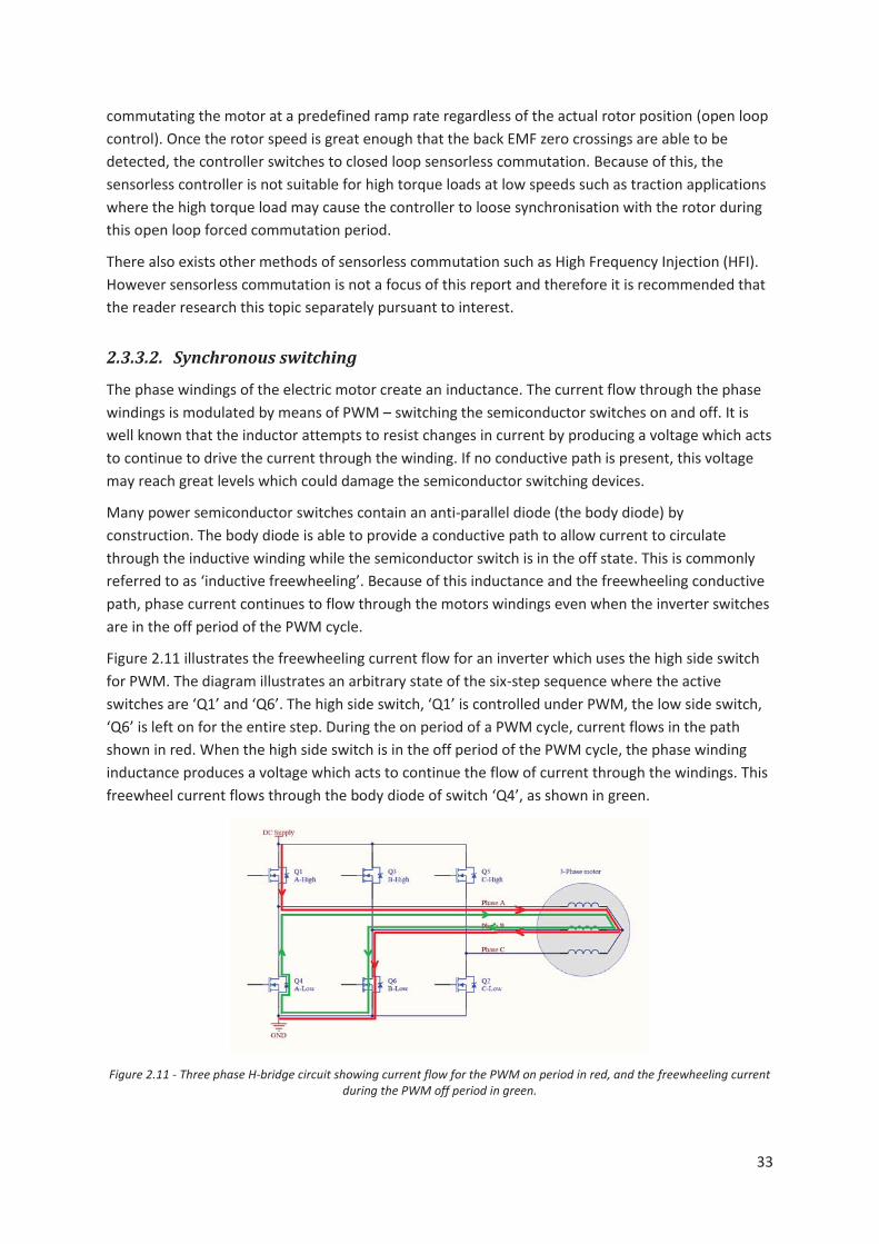
33
commutating the motor at a predefined ramp rate regardless of the actual rotor position (open loop control). Once the rotor speed is great enough that the back EMF zero crossings are able to be detected, the controller switches to closed loop sensorless commutation. Because of this, the sensorless controller is not suitable for high torque loads at low speeds such as traction applications where the high torque load may cause the controller to loose synchronisation with the rotor during this open loop forced commutation period.
There also exists other methods of sensorless commutation such as High Frequency Injection (HFI). However sensorless commutation is not a focus of this report and therefore it is recommended that the reader research this topic separately pursuant to interest.
2.3.3.2. Synchronous switching
The phase windings of the electric motor create an inductance. The current flow through the phase windings is modulated by means of PWM – switching the semiconductor switches on and off. It is well known that the inductor attempts to resist changes in current by producing a voltage which acts to continue to drive the current through the winding. If no conductive path is present, this voltage may reach great levels which could damage the semiconductor switching devices.
Many power semiconductor switches contain an anti-parallel diode (the body diode) by construction. The body diode is able to provide a conductive path to allow current to circulate through the inductive winding while the semiconductor switch is in the off state. This is commonly referred to as ‘inductive freewheeling’. Because of this inductance and the freewheeling conductive path, phase current continues to flow through the motors windings even when the inverter switches are in the off period of the PWM cycle.
Figure 2.11 illustrates the freewheeling current flow for an inverter which uses the high side switch for PWM. The diagram illustrates an arbitrary state of the six-step sequence where the active switches are ‘Q1’ and ‘Q6’. The high side switch, ‘Q1’ is controlled under PWM, the low side switch, ‘Q6’ is left on for the entire step. During the on period of a PWM cycle, current flows in the path shown in red. When the high side switch is in the off period of the PWM cycle, the phase winding inductance produces a voltage which acts to continue the flow of current through the windings. This freewheel current flows through the body diode of switch ‘Q4’, as shown in green.
Figure 2.11 - Three phase H-bridge circuit showing current flow for the PWM on period in red, and the freewheeling current
during the PWM off period in green.

34
The body diode of the semiconductor switches has a forward voltage drop, Vf. The power dissipated, Pfw as heat across the body diode during freewheel current flow, Iphase (for the duration of the PWM off state) is simply calculated as:
(2.66)
Often this power dissipation is greater than what it would be if the semiconductor switch was in the ‘on’ state and the freewheel current allowed to circulate through the switch instead of the body diode. In this case, the power dissipated as heat in the semiconductor switch across its on resistance, Ron would be:
(2.67)
As an example, a modern power transistor was selected, the “IRFS7530” and the freewheeling power dissipation was calculated for the case where body diode conduction is used and the case where semiconductor switch conduction is used for the freewheel current, as shown in Figure 2.12.
Figure 2.12 - Plot of the power dissipated as heat in the semiconductor switch during freewheel current flow through the body diode and the semiconductor switch for the “IRFS7530” transistor.
Clearly there is a significant advantage in turning on the semiconductor switch for the periods in which it would be circulating freewheel current. This is often implemented in Six-step motor controllers and is referred to as ‘synchronous switching’ or ‘active freewheeling’.
In the case shown in Figure 2.11, the high side switch of phase A is being used for PWM. To perform synchronous switching, the low side switch of the same phase must be turned on during the high side switch off period. Therefore synchronous switching may be performed by implementing a complementary PWM controller for each of the phases high and low side switches.
0
20
40
60
80
100
120
0 10 20 30 40 50 60 70 80 90 100
110
120
130
140
150
160
170
180
190
200
210
220
230
240
Pow
er D
issip
atio
n [W
]
Phase Current [A]
Freewheel Power Dissipation for IRFS7530
Body diode
Switch

35
2.3.3.3. Dead-time
Again referring back to Figure 2.11, we can see that if there were a time when the high and low side switches of a single phase were both turned on, there would be a short circuit created between the DC supply and GND through the switches. This would almost instantly blow the semiconductor switches unless there is some form of over current protection.
Now consider the case where complementary PWM is used between the high and low side switches for the purpose of synchronous switching. Clearly the high side switch must be fully in the off state before the low side switch of that same phase is turned on. The gate drive circuitry takes some non-trivial amount of time to discharge the gate charge in order to turn off the semiconductor switch. Similarly, the gate drive circuitry takes some non-trivial time to charge the gate charge to turn on the low side switch. If both the high side and low side were given these turn off/on signals at the same instant, there would be some overlapping time period where there is conduction from the DC supply through both the high and low side switches to GND while the on/off transition completes. The same holds true for when the high side switch is turned back on for the PWM ‘on’ period.
The duration that conduction occurs through the high side and low side switches may be very short as to not blow the transistors, however it is obviously non-desirable as it results in a power loss across the switches which occurs at both the turn off and turn on events of each PWM cycle (twice the PWM frequency).
For this reason, dead-time should be inserted between high side and low side switching events so that the switching transition times are allowed for. This may be done in software or in hardware.
2.3.4. Field Oriented Control
Field Oriented Control (FOC) (or synonymously referred to as Vector Control) is a well-established method of control for three phase AC machines. FOC aims to directly control the torque producing current, Iq and magnetic field producing current, Id as two decoupled quantities. The FOC algorithm in block diagram representation is illustrated in Figure 2.13.
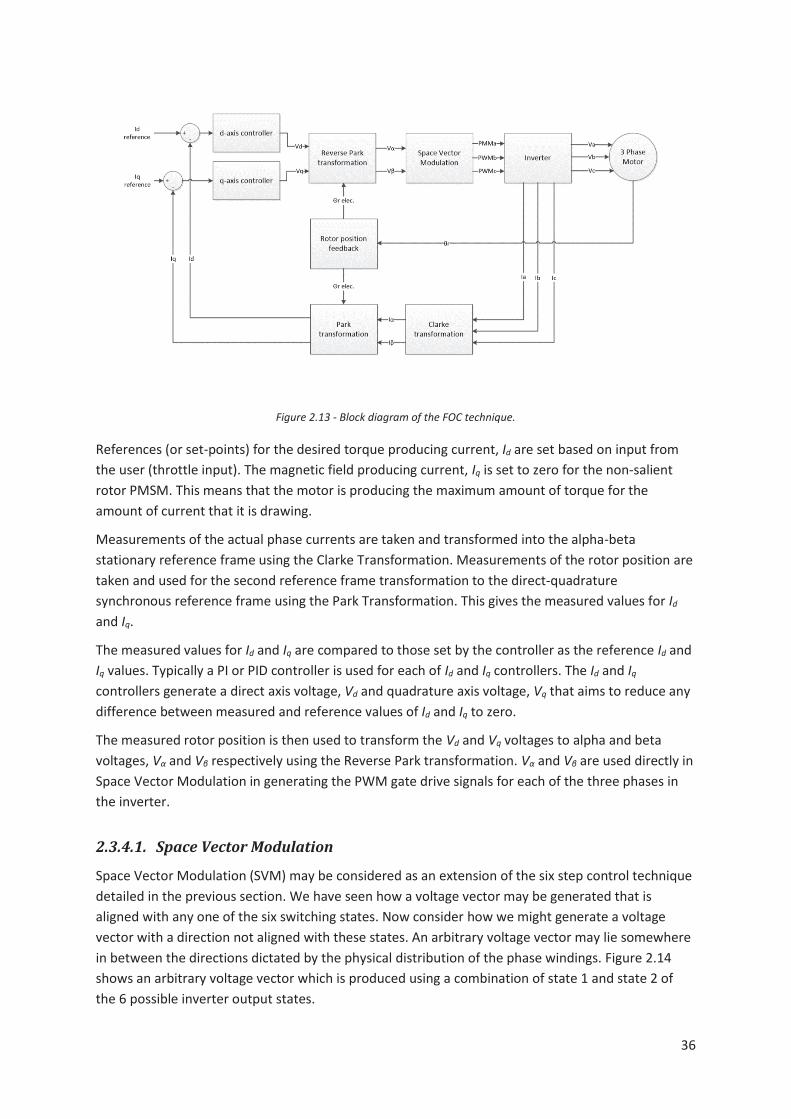
36
Figure 2.13 - Block diagram of the FOC technique.
References (or set-points) for the desired torque producing current, Id are set based on input from the user (throttle input). The magnetic field producing current, Iq is set to zero for the non-salient rotor PMSM. This means that the motor is producing the maximum amount of torque for the amount of current that it is drawing.
Measurements of the actual phase currents are taken and transformed into the alpha-beta stationary reference frame using the Clarke Transformation. Measurements of the rotor position are taken and used for the second reference frame transformation to the direct-quadrature synchronous reference frame using the Park Transformation. This gives the measured values for Id and Iq.
The measured values for Id and Iq are compared to those set by the controller as the reference Id and Iq values. Typically a PI or PID controller is used for each of Id and Iq controllers. The Id and Iq controllers generate a direct axis voltage, Vd and quadrature axis voltage, Vq that aims to reduce any difference between measured and reference values of Id and Iq to zero.
The measured rotor position is then used to transform the Vd and Vq voltages to alpha and beta voltages, Vα and Vβ respectively using the Reverse Park transformation. Vα and Vβ are used directly in Space Vector Modulation in generating the PWM gate drive signals for each of the three phases in the inverter.
2.3.4.1. Space Vector Modulation
Space Vector Modulation (SVM) may be considered as an extension of the six step control technique detailed in the previous section. We have seen how a voltage vector may be generated that is aligned with any one of the six switching states. Now consider how we might generate a voltage vector with a direction not aligned with these states. An arbitrary voltage vector may lie somewhere in between the directions dictated by the physical distribution of the phase windings. Figure 2.14 shows an arbitrary voltage vector which is produced using a combination of state 1 and state 2 of the 6 possible inverter output states.
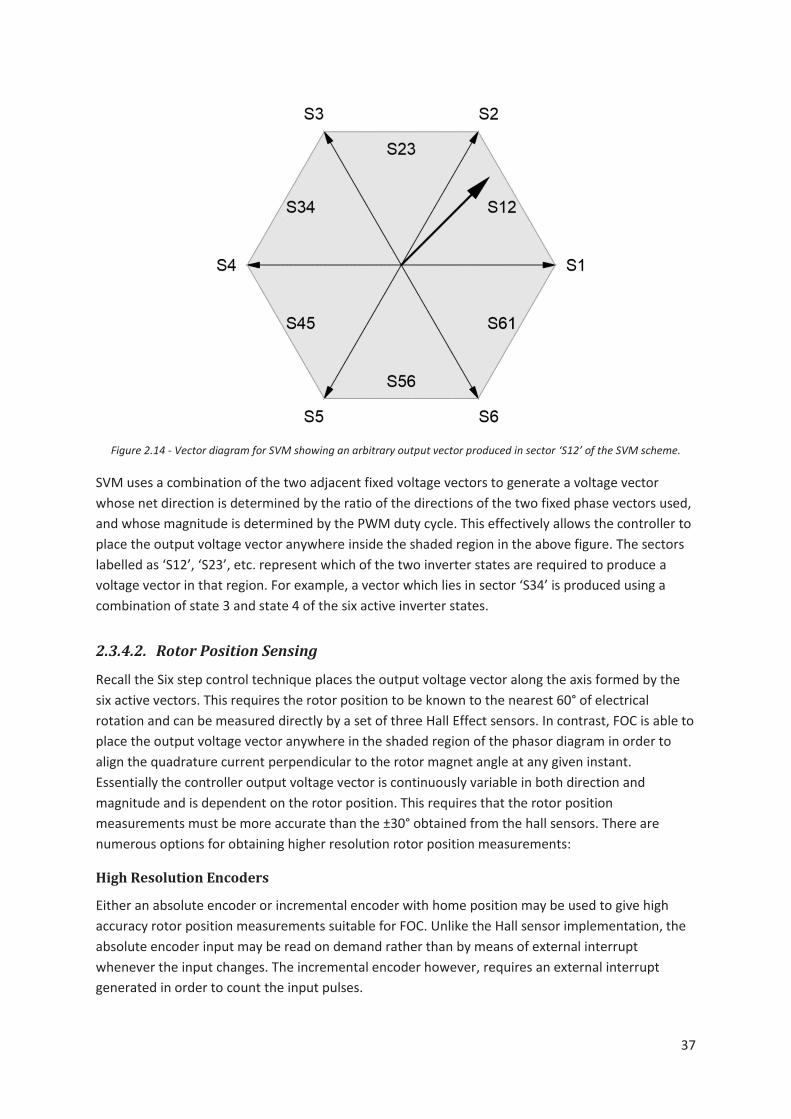
37
Figure 2.14 - Vector diagram for SVM showing an arbitrary output vector produced in sector ‘S12’ of the SVM scheme.
SVM uses a combination of the two adjacent fixed voltage vectors to generate a voltage vector whose net direction is determined by the ratio of the directions of the two fixed phase vectors used, and whose magnitude is determined by the PWM duty cycle. This effectively allows the controller to place the output voltage vector anywhere inside the shaded region in the above figure. The sectors labelled as ‘S12’, ‘S23’, etc. represent which of the two inverter states are required to produce a voltage vector in that region. For example, a vector which lies in sector ‘S34’ is produced using a combination of state 3 and state 4 of the six active inverter states.
2.3.4.2. Rotor Position Sensing
Recall the Six step control technique places the output voltage vector along the axis formed by the six active vectors. This requires the rotor position to be known to the nearest 60° of electrical rotation and can be measured directly by a set of three Hall Effect sensors. In contrast, FOC is able to place the output voltage vector anywhere in the shaded region of the phasor diagram in order to align the quadrature current perpendicular to the rotor magnet angle at any given instant. Essentially the controller output voltage vector is continuously variable in both direction and magnitude and is dependent on the rotor position. This requires that the rotor position measurements must be more accurate than the ±30° obtained from the hall sensors. There are numerous options for obtaining higher resolution rotor position measurements:
High Resolution Encoders
Either an absolute encoder or incremental encoder with home position may be used to give high accuracy rotor position measurements suitable for FOC. Unlike the Hall sensor implementation, the absolute encoder input may be read on demand rather than by means of external interrupt whenever the input changes. The incremental encoder however, requires an external interrupt generated in order to count the input pulses.

38
Hall Sensor Extrapolation
This technique involves timing the duration between changes in the Hall sensor input. With this information, the rotor speed can be calculated and updated after each time the input toggles i.e. every 60° of electrical rotation. With the measurement of the rotor speed from the previous 60° of electrical rotation, the current rotor angle may be estimated to a high resolution by extrapolating from the last hall input change.
Sensorless Methods
There are various sensorless methods of measuring the rotor position to a high resolution for FOC. The previously mentioned High Frequency Injection (HFI) may be used or other methods such as ‘Phase Locked Loop (PLL) Observer’ or ‘Cordic Observer’. The reader is encouraged to research these methods separately pursuant to interest.
2.3.5. Comparison of Six-Step Control and FOC
To summarise, Six-Step Control is a basic motor control technique that works by stepping through a sequence of six inverter output states based on commutation events. The inverter is able to produce a voltage vector which has a direction aligned with any one of the six discrete states which have an electrical spacing of 60°. The magnitude of the voltage vector is modulated using PWM.
The result of this is that at any instant, the three phase motor is being driven by a voltage vector which is anywhere from 30° lagging or 30° leading the optimal torque producing vector direction. Consider the movement of the rotor magnet angle through 60° of rotation. At the instant when the magnet angle is exactly perpendicular to the applied voltage vector, the output torque will reach a maximum for the given amount of motor current. As the rotor continues to rotate past the direction of the applied voltage vector, the amount of torque will decrease for the same amount of motor current. As the perpendicular rotor angle reaches half way to the next voltage vector direction, the commutation is triggered, switching the inverter to the next state. The motor torque will then begin to increase again until it reaches its maximum when the magnet angle is perpendicular to the new inverter output voltage vector. It is clear that this motor control scheme introduces torque ripple which occurs at a frequency of six times the electrical revolution frequency.
In contrast, FOC operates by applying an output voltage vector which is in theory, able to modulate both the direction and magnitude as a continuously variable output. This means that it can not only eliminate torque ripple, but also drive the motor such that torque production is maximised for a given motor current.
As discussed previously in 2.2.4, the motor equations are complex. The optimal voltage vector cannot be determined based on the rotor position alone. The motor equations are modelled in the FOC algorithm to calculate the measured torque producing current, Iq, and field current, Id. PID controllers (or similar) are used to adjust the output of the inverter in an attempt to achieve a field current of zero amps so that torque producing current is maximised.

39
3. Prototype Design
This section discusses design considerations around building the prototype LEV. The author has a particular interest in electric powered skateboards and therefore a prototype has been build based on a ‘longboard’ style of skateboard. This allows for rapid and cost effective prototype testing of the hub motors and motor controllers. The electric skateboard application does not require high levels of power output from the electric motor and motor controller and therefore it also does not require a high capacity battery pack. Low power requirements means the cost of components is relatively low. These factors make the electric skateboard a feasible LEV on which this Masters project is focuses on.
3.1. Design Considerations
As an engineering project in the final year of the Bachelor of Engineering Degree, the author built a Six-Step Motor Controller along with a ‘mountain board’ style electric powered skateboard. This LEV prototype was built for the purposes of allowing extreme sport enthusiasts to take the sport of mountain boarding to flat or even uphill slopes, rather than being limited to downhill only. A photograph of the electric powered mountain board is given in Figure 3.1.
Figure 3.1 - Electric mountain board prototype built as part of final year engineering project.
A paper was written on this project titled “Instrumentation and Control of a High Power BLDC Motor for Small Vehicle Applications”. This was published in the IEEE International Instrumentation and Measurement Technology Conference (I2MTC 2012):
40
Alexander Rowe, Gourab Sen Gupta, Serge Demidenko, “Instrumentation and Control of a High Power BLDC Motor for Small Vehicle Applications”, Proceedings of the IEEE International Instrumentation and Measurement Technology Conference (I2MTC 2012), Graz, Austria, May 14–16, 2012, pp.559-564
Abstract:
Brushless DC (BLDC) motors are becoming an increasingly popular motor of choice for low powered vehicles such as mopeds, power assisted bicycles, mobility scooters, and in this reported application, motorised mountain boards. With rapid developments in technology, high energy density batteries such as Lithium-ion Polymer batteries are becoming more affordable and highly suitable for such vehicles due to the superior charge rate and light weight of the lithium chemistry batteries. This combined with the high power, light weight, and cheap BLDC motor results in the BLDC motor being a very favourable solution over an internal combustion (IC) engine for low power vehicles with power requirements of up to 7kW. A BLDC motor controller was developed specifically for the motorised mountain board application. The motor controller is a ‘sensored’ BLDC motor controller which takes inputs from Hall Effect sensors installed inside the motor to determine the motor position. Many other sensors are used to monitor the variables that are critical to the operation of the motor controller such as the motor phase current, battery voltage, motor temperature, and transistor temperature. The reported system is further enhanced by several additional features such as output for an LCD screen, regenerative braking, timing advance, cruise control, and soft start functions. These topics are discussed briefly in this paper.
The full journal article is provided in Appendix A.
Following from the electric mountain board prototype, a second prototype electric skateboard was designed and built as part of this Masters project. This second prototype was designed to address the key issues identified in the first prototype phase.
3.1.1. Motor Controller
The motor controller would frequently blow transistors due to limitations of the chosen microcontroller causing delays in commutations. The motor controller was also large in size as there had been limited efforts to design for minimal size of the circuit board.
The second prototype incorporates a completely re-designed motor controller with a high performance 32-bit microcontroller. This allowed for the study of advanced motor control techniques as discussed in section 2.3.
3.1.2. Turning Radius
The mountain board was designed for off road use, on surfaces such as grass, gravel, dirt, etc. and therefore a two wheel drive design was chosen for the purposes of increased traction on loose surfaces such as gravel, and to eliminate the unwanted torque-steer that is an inherent property of one wheel drive terrains. The electric mountain board uses a single motor to drive both of the rear wheels. It does not allow for the rear wheels to rotate at differential speeds; the two rear wheels are indirectly coupled together through the motor shaft.

41
While the electric mountain board handles well for its intended purpose of off road use on surfaces that allow for some wheel slip while cornering, the design falls short in on-road use. On high traction surfaces such as sealed roads or footpaths there is no wheel slip while cornering and therefore makes the handling on such surfaces difficult as there is a very large turning radius.
A major consideration for this project was to eliminate the issue outlined above. A simple and cost effective solution was to use two separate, smaller motors to drive each rear wheel separately.
The decision to keep the skateboard as two-wheel drive comes from the fact that a one-wheel drive system would suffer from torque-steer; when accelerating or breaking, the force on the wheel due to motor torque would cause the skateboard to turn and therefore the handling of the electric skateboard would suffer.
3.1.3. Size and Weight
The electric mountain board was heavy and bulky. The second prototype was designed to be smaller and lighter in order to make it more practical for everyday use such as short commutes. With this in mind, the decision was made to use a ‘longboard’ style of skateboard as the basis for second prototype of the electric skateboard for this Masters project.
The longboard is physically smaller in overall dimensions and significantly lighter which makes it easier to carry, making it more practical as a mode of transportation. In contrast, the electric mountain board which was found to be useful for recreational use only.
3.1.4. Hub Motor Design
A typical electric skateboard uses a belt or chain drive to transfer power from the motor to the wheel. This allows for an appropriate gear ratio to be selected in order to increase the torque and reduce the speed from the motor to the wheel.
In an attempt to simplify the design of the electric longboard, an innovative hub motor design was chosen. This eliminates the need for a belt or chain reduction drive which reduces cost, weight, maintenance, and complexity of manufacture and assembly. A hub motor is simply an “outer-rotor” motor with the wheel attached to the outside of the rotor, and the stator fixed in the centre of the wheel.
A direct drive hub motor offers numerous advantages over the commonly used belt or chain reduction drive as well as some disadvantages, as summarised in Table 3.1.

42
Advantages Disadvantages
Reduces complexity – No motor mounts, no tensioning system
More limitations on motor selection – must be “outer rotor” and must produce sufficient torque to drive the wheel directly.
Reduces cost – less components to purchase and manufacture
Limits wheel size – no speed reduction through gearing
Reduced weight – less components Limits Battery voltage – no speed reduction through gearing
Reduced maintenance – no belt to tension and occasionally replace, no periodic chain lubrication
The motor spins at a lower speed therefore the motor and motor controller combination inherently are a lower voltage, higher current system – resistive power loss is greater
No power loss in power transmission.
Table 3.1 - Comparison of the advantages and disadvantages of a hub motor setup over a reduction drive setup.
The disadvantages of the hub motor drive are largely to do with creating more limitations on component selection. However, if a suitable combination of motor, battery configuration, and motor controller is available at a similar cost to that of the components required for a belt or chain drive setup, then the hub motor system could prove advantageous.
3.1.5. Physical Layout of Equipment
The electric mountain board prototype was designed for off road use and therefore the additional equipment was placed so that it would not compromise the overall clearance. As a result, the batteries and motor controller were placed on the top side of the skateboard deck, placed in between where the user’s feet would usually be positioned. The motor was mounted behind the rear wheels.
The difficulty with this layout is that the user must place their feet in fixed positions on the skateboard deck, and would often trip on the equipment when unexpectedly having to dismount the electric mountain board.
The longboard style of skateboard is designed for on road use (sealed surfaces) due to its smaller, solid rubber wheels. The electric longboard prototype adopts an equipment layout that places all of the electrical equipment on the underside of the deck therefore eliminates the tripping hazard. The layout was also selected to be as flat as possible so that it does not have a large effect on the clearance of the longboard.
3.1.6. Handheld Controller
The handheld controller from the electric mountain board prototype used a cable connection to communicate with the motor controller. Having this cable connection was fond to be cumbersome as it restricted movement of the user.

43
The electric longboard prototype addressed this issue by using a wireless handheld controller. For simplicity, a RC transmitter and receiver was used. The transmitter takes an analogue input from the ‘throttle’ potentiometer and transmits the throttle value via digital radio on the 2.4GHz band. The receiver detects this signal and outputs a digital PWM signal to the motor controller.
The disadvantage of this ‘off the shelf’ handheld controller is that there is no customisable display of data as there was on the original handheld controller LCD. Instead, a power meter was installed in the electric longboard to display and record data such as battery capacity consumed, current, voltage, power, speed, and temperatures.
3.2. Power Requirement Modelling
The electric longboard prototype LEV was intended as an on-road vehicle and therefore a target top speed was selected as 50km/h. It was also desired that the longboard should be able to travel up hills without effecting the speed too much. With this in mind, a design target speed of 50km/h up a 10° angle of incline was selected. The electric longboard should be capable of travelling a distance that would exceed the users typical range requirements on a single battery charge. For the propose of quantifying this statement the range objective was defined as 20km distance at an average speed of 40km/h on an overall flat route.
A Matlab model was produced to predict the power requirements for the electric longboard. The script source code is provided in Appendix B. Note that the selection of equipment was carried out in conjunction with the development of the Matlab model. Initial estimates of input variables were updated with specific values from datasheets for the individual components as each component was selected. The model was also used in making comparisons of the expected performance of different components.
3.2.1. Model Formulae
The model takes into account the significant forces required to propel the electric skateboard as well as the significant energy losses in the system. The total mechanical load is calculated as a sum of wind resistance, rolling resistance, and the torque required to gain height when used in an uphill scenario. The model also accounts for the major power losses of resistive power loss in the battery, resistive and switching power loss in the inverter, and resistive, hysteresis, and eddy current power losses in the motor.
The force to overcome aerodynamic drag is calculated by
(3.1)
The force required to overcome rolling resistance is calculated by the following equation. It is assumed that the total mass is spread evenly across four wheels.

44
(3.2)
The force required to gain height for a given angle of incline, θ is calculated by
(3.3)
The total mechanical load is the sum of these mechanical forces and is converted to a torque load by multiplying the total force by the radius of the wheel.
(3.4)
The total mechanical power is calculated as the total mechanical torque multiplied by the angular velocity of the wheels, ω.
(3.5)
Where angular speed, ω is calculated using the wheel diameter, D and the linear speed, v according to equation (3.6).
(3.6)
The total mechanical load is shared evenly between two motors, and the current through each motor, I1 is calculated using the motor constant, km.
(3.7)
And voltage required, V for a given speed is calculated as
(3.8)
The electrical power required is calculated as the sum of the mechanical load and the electrical power losses in the system. Discrete power losses are identified as follows.
A single battery pack supplies the total current required for both motors. The power loss, Pbatt due to the internal resistance of the battery, Rb is given by
(3.9)
Similarly to the motors, the total load is shared even between two motor controllers. The power loss in each of the inverters is a combination of resistive losses and switching losses. To simplify the mathematics, it will be assumed that the inverter is being operated under the Six-Step Control technique and therefore two switches are active at a given time and the multiplier of two is used. Also synchronous switching is assumed therefore there are no freewheel diode loss to account for and the resistive power loss is applied across the full PWM cycle so there is no need to estimate the duty cycle.
45
(3.10)
The switching losses are much more complicated in nature however a simplified analysis can be obtained using an idealised approximation for the turn-on and turn-off switching times of the semiconductor switches. The well-known Resistive-capacitive time constant can be applied to the gate capacitance of the transistor to model the gate voltage (Markowski, 2002).
The resistive-capacitive time constant, TRC is calculated using the total gate resistance, Rgate as seen by the gate driver circuitry, and the gate capacitance obtained from the total gate charge, Qgate as given in the device manufacturer’s datasheet and the selected gate drive voltage, Vdrive.
(3.11)
The equation for modelling the gate to source voltage, Vgs during the charging of the resistive-capacitive circuit is given by the formula
(3.12)
Rearranging gives
(3.13)
The gate voltage threshold is the voltage at which the transistor is considered to be fully ‘on’, and is given in the device datasheet. The turn-on time can then be obtained by substituting values for the gate turn-on threshold voltage, gate drive voltage, total gate resistance, and total gate capacitance. The turn-on switching power loss occurs once every cycle of the switching frequency. The formula for this idealised switching loss is (Markowski, 2002)
(3.14)
To turn off the transistor, the charge from the gate capacitance needs to discharge through the same gate resistance (assuming that the gate driver configuration does not have an additional conductive path for the gate capacitance discharge). Therefore the transistor turn off time can be assumed to be the same as the turn on time so a multiplier of two is used to estimate the total switching power loss.
(3.15)
Also associated with the switching loss is the power used in charging the gate capacitance and in the parasitic output capacitance of the MOSFET. This power loss is expressed in the following equation where the first term is the power loss due to parasitic output capacitance and the second term is power loss due to gate capacitance.
46
(3.16)
Co is the parasitic output capacitance of the MOSFET and is obtained from the manufactures datasheet, Vbatt is the battery voltage (or the inverter bus voltage), fsw is the PWM switching frequency, Qg is the MOSFET total gate charge and is obtained from the datasheet, and Vgate is the gate drive voltage.
Note that all these parameters are fixed with the exception of battery voltage which decreases as the battery is discharged. However using the nominal battery voltage for this parameter, a good approximation can be reached. In this case, the capacitive switching power loss is a constant and is calculated to be 0.099W for the selected components and switching frequency of 20kHz.
Diode power loss is calculated given the time spent in conduction. The motor control algorithms investigated in this project use techniques to minimise the amount of time that the body diode is conducting the ‘freewheel’ currents and therefore the power loss. This is achieved by using the synchronous switching technique which turns on the transistor that would otherwise be conducting freewheel current, so that current flow is through the transistor rather than the body diode. However, there is still a small time period where the body diode is conducting during switching transitions in the dead-time period. This power loss period occurs during the switch on and the switch off transition therefore two times for each PWM cycle.
(3.17)
Where I1 is the current through the single transistor, Vf is the forward voltage drop of the MOSFET body diode, tDT is the dead-time, and fsw is the switching frequency.
And the total power loss in each inverter is the sum of the resistive and switching power loss.
(3.18)
The power loss in each motor, Pmotor is calculated as the sum of ‘Copper Loss’, eddy current loss, and hysteresis loss as given in the following equation.
(3.19)
Where the peak magnetic flux density, Bp is calculated using the following equation adapted from (Jiles, 1998)
(3.20)
Where μ is the permeability of the core material which can be obtained from datasheets, I1 is the electrical current flowing through the coil, N is the number of turns in the coil, and L is the stator length.
The total electrical power required is given as the sum of the mechanical power and all electrical power losses, noting that there are two motors and two inverters for this configuration.

47
(3.21)
Efficiency of the system is calculated as the ratio of power input to the power output.
(3.22)
3.2.2. Matlab Model
A Matlab script was produced which models the system using a list of constant parameters as inputs to the equations from the previous section.
The code uses two nested ‘for’ loops to step through a specified range of discrete values for angle of incline on the outer loop, and speed on the inner loop. As each new value for angle of incline or speed is generated, the program calculates the total power required, efficiency, and the expected range for the given speed and angle of incline. The output data is stored in two dimensional arrays which are used to plot graphs.
Figure 3.2 shows the total power requirement as a function of speed for six discrete angle of incline slopes. This estimates that 3.4kW of power is required to achieve the project objective of the electric longboard being capable of travelling at a speed of 50km/h up a 10° angle of incline.
Figure 3.2 - MATLAB Model simulation of the power requirements for the electric longboard as a function of speed and
various angles of incline.
The range prediction is dependent on the battery energy capacity. The simulation was used to calculate the energy capacity required to achieve the objective of being capable of travelling 20km at 40km/h. It was found that the battery energy capacity must be at least 312Wh. The simulation was run for the selected battery pack of 444Wh energy capacity (22.2V, 20Ah) and predicted a range of 27.7km at a speed of 40km/h. Figure 3.3 shows the expected range of the electric longboard for a given speed and angle of incline.
0 10 20 30 40 50 600
0.5
1
1.5
2
2.5
3
3.5
4
4.5
X: 50.4Y: 3.441
Power requirement predictions
Velocity [km/h]
Pow
er [k
W]
0 deg2 deg4 deg6 deg8 deg10 deg

48
Figure 3.3 - MATLAB model simulation of the range predictions as a function of speed and various angles of incline.
Contrary to general expectations, the maximum range is not realised at a speed where the electric skateboard is only just moving at an infinitesimally small speed. This is largely due to the rolling resistance of the wheels which requires a constant torque to overcome. Also worth noting is that the curves on the graph above pass through the origin (0,0) point. This represents the scenario there the inverter is supplying current to the motor but does not produce sufficient torque to overcome rolling resistance and therefore the resulting range is 0km at 0km/h.
3.3. Equipment Selection
As discussed in the previous section, the electric skateboard prototype is based on a longboard style of skateboard using a direct drive hub motor design. The selection a suitable combination of electrical equipment is a crucial element effecting the overall performance of the electric skateboard prototype. In addition to this, the longboard parts; wheels, trucks, and deck must be selected taking into account how the electrical equipment is going to be physically located and attached for the desired application. This section gives a breakdown of the selection process for the individual parts of the electric longboard, however parts were not selected in isolation; an overall understanding of the range of parts commercially available is required to ensure a suitable combination of equipment is reached. As an example, it was desirable to keep the electronic equipment on the underside of the deck as thin as possible as to keep the overall clearance of the electric skateboard at a reasonable level. This design consideration effects both battery selection and motor controller selection.
It should be noted that equipment was selected to meet the project objective of being able travel at 50km/h up a 10° slope as non-continuous operation (burst power). It was not intended that the prototype electric longboard would be able to operate under these conditions for an extended period of time; a typical and more realistic expectation is that the user would travel at a speed of around 40km/h on an overall flat route. Therefore the equipment was selected that would be able to withstand high power output for short periods of time – for example while accelerating or
0 10 20 30 40 50 600
10
20
30
40
50
60
X: 40.2Y: 27.65
Range predictions
Velocity [km/h]
Dis
tanc
e [k
m]
0 deg2 deg4 deg6 deg8 deg10 deg
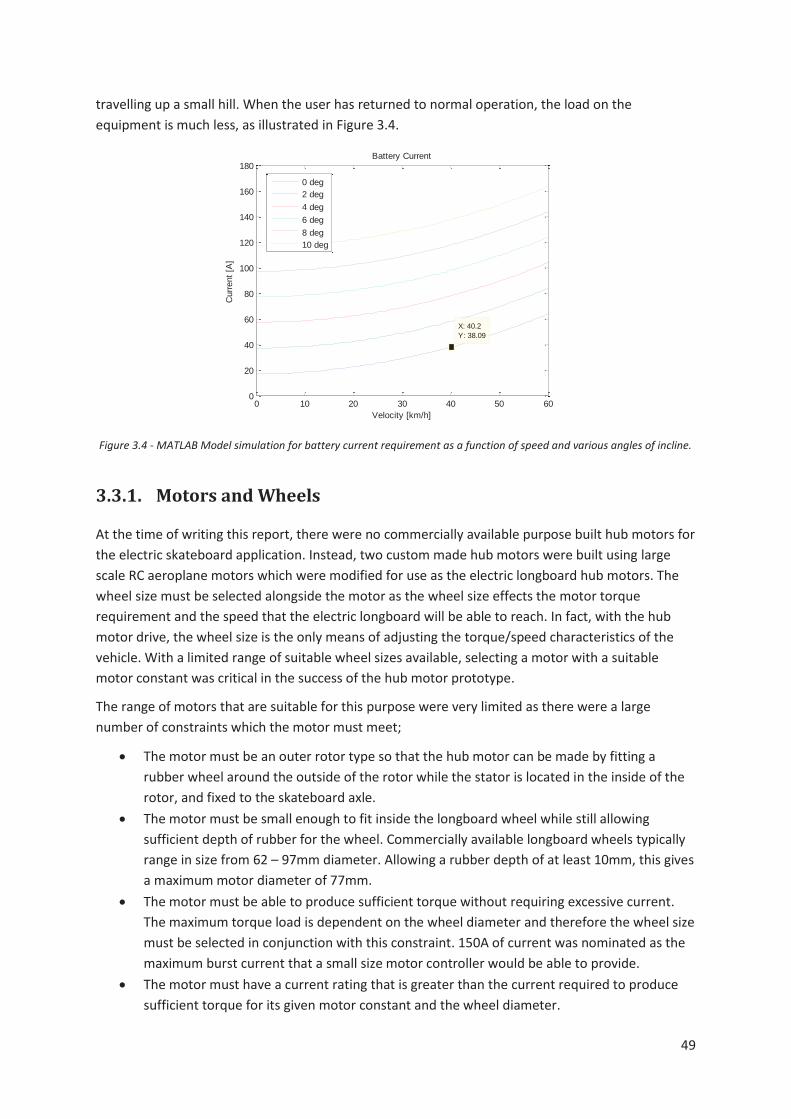
49
travelling up a small hill. When the user has returned to normal operation, the load on the equipment is much less, as illustrated in Figure 3.4.
Figure 3.4 - MATLAB Model simulation for battery current requirement as a function of speed and various angles of incline.
3.3.1. Motors and Wheels
At the time of writing this report, there were no commercially available purpose built hub motors for the electric skateboard application. Instead, two custom made hub motors were built using large scale RC aeroplane motors which were modified for use as the electric longboard hub motors. The wheel size must be selected alongside the motor as the wheel size effects the motor torque requirement and the speed that the electric longboard will be able to reach. In fact, with the hub motor drive, the wheel size is the only means of adjusting the torque/speed characteristics of the vehicle. With a limited range of suitable wheel sizes available, selecting a motor with a suitable motor constant was critical in the success of the hub motor prototype.
The range of motors that are suitable for this purpose were very limited as there were a large number of constraints which the motor must meet;
The motor must be an outer rotor type so that the hub motor can be made by fitting a rubber wheel around the outside of the rotor while the stator is located in the inside of the rotor, and fixed to the skateboard axle.
The motor must be small enough to fit inside the longboard wheel while still allowing sufficient depth of rubber for the wheel. Commercially available longboard wheels typically range in size from 62 – 97mm diameter. Allowing a rubber depth of at least 10mm, this gives a maximum motor diameter of 77mm.
The motor must be able to produce sufficient torque without requiring excessive current. The maximum torque load is dependent on the wheel diameter and therefore the wheel size must be selected in conjunction with this constraint. 150A of current was nominated as the maximum burst current that a small size motor controller would be able to provide.
The motor must have a current rating that is greater than the current required to produce sufficient torque for its given motor constant and the wheel diameter.
0 10 20 30 40 50 600
20
40
60
80
100
120
140
160
180
X: 40.2Y: 38.09
Battery Current
Velocity [km/h]
Cur
rent
[A]
0 deg2 deg4 deg6 deg8 deg10 deg

50
The motor must be powerful enough to meet the design objective of being capable of travelling at 50km/h up a 10° incline. This power requirement is shared across two motors therefore the power rating of each motor must be at least 1546W.
The motor must be rated for a battery voltage that high enough to achieve a speed of 50km/h for its motor speed constant and wheel diameter.
The motor must be constructed with bearings directly supporting the rotor assembly at both ends of the motor. Note that outer rotor type PMSM typically have a shaft attached to the rotor which is supported by bearings at both ends (a cross section is provided in Figure 3.8). In a hub motor application, the load on the rotor is largely a radial load and therefore the motor selection is limited to those that have bearing support at both ends of the rotor cylinder.
A Microsoft Excel spreadsheet was created to compare a number of suitable motor candidates. Calculated columns were used to perform calculations for the motor’s specific power rating, current required to produce the desired torque, and the speed that the motor will run at for a specific battery voltage and wheel diameter. It also allowed for comparison of motor ratings and costs.
This lead to the selection of the “Turnigy SK3 6374-149” for the electric longboard hub motor in combination with a 90mm diameter wheel size as it meets all of the motor selection criteria and is able to produce the required torque with the lowest amount of current (high motor constant). This particular motor uses a “Distributed-LRK” (DLRK) motor winding scheme with a 14 magnet pole rotor. The specifications are listed in Table 3.2 below:
Specification Value Units
Motor diameter 59 mm
Motor length 61 mm
Power rating 2250 W
Current rating 80 A
Voltage rating 44 V
Motor constant 0.064 Nm/A
Motor speed constant 149 RPM/V
Phase resistance 0.021 Ω
Weight 840 g
Winding scheme DLRK Delta -
Magnet poles 14 -
Table 3.2 - Electric longboard motor specifications.

51
These values were inserted into the Matlab simulation which was then used to generate a plot of predicted power loss in a single motor over the design speed and angle of incline range, as given in Figure 3.5. The simulation predicts that the motors will each dissipate 190W of heat at 50km/h up a 10° incline.
Figure 3.5- MATLAB Model simulation for the power loss in each of the two motors as a function of speed and various
angles of incline.
The longboard trucks were also selected specifically for the hub motor design. “Paris V2 180mm” trucks were selected to allow for easy installation of the hub motors as they are constructed with a cylindrical axle which the hub motor stator would fit over with minimal modifications.
3.3.2. Battery Selection
The batteries for the electric longboard were selected based on the following criteria:
The individual batteries must be able to be arranged such that the overall height of the complete battery pack does not exceed 40mm, and fit within the area of the longboard deck underside which is 160mm wide and 550mm long.
The resulting battery pack must have a nominal voltage that will allow the motors to reach a speed of no less than 50km/h. Given the motor speed constant of 149 RPM/V and the wheel diameter of 90mm, it can be calculated that the battery must have a nominal voltage of no less than 21.9V, assuming that the loaded speed will reach 90% of the un-loaded speed.
The resulting battery pack must have sufficient energy capacity to meet the range objective of 20km at a speed of 40km/h on an overall flat route, which was calculated to be 328Wh of energy.
The resulting battery pack must be rated to supply sufficient current to achieve the required motor torque of 5Nm for each motor. Given the selected motors have a motor constant of 0.064Nm/A, the battery pack must have a current rating of at least 156A.
A range of batteries which meet the above criteria were evaluated comparing gravimetric energy density, volumetric density, and cost per Watt-hour of energy capacity. Again, Microsoft Excel was a
0 10 20 30 40 50 600
50
100
150
200
250
X: 50.4Y: 190.4
Power loss in each motor
Velocity [km/h]
Pow
er lo
ss [W
]0 deg2 deg4 deg6 deg8 deg10 deg

52
useful tool in comparing the battery options. The battery selected is the “Turnigy Lithium Polymer 5Ah 3S 20C” battery due to it having the lowest cost per Watt-hour of energy capacity and having very high gravimetric and volumetric energy density. To achieve a nominal battery pack voltage of greater than 21.9V, two of these batteries are connected in series. To achieve the energy capacity of greater than 328Wh, four lots of two series connected batteries are connected in parallel. This gives the battery pack configuration as ‘6S4P’, and is made up of eight separate three cell batteries. The specifications of the battery pack are listed in Table 3.3.
Specification Value Units
Voltage (nominal) 22.2 V
Minimum voltage 19.2 V
Maximum voltage 25.2 V
Maximum discharge rate 400 A
Maximum charge rate 20 A
Capacity 20 Ah
Energy Capacity 444 Wh
Internal resistance 0.0055 Ω
Weight 3.296 kg
Dimensions 392(L) x 145(W) x 26(H) mm
Table 3.3 - Electric longboard battery specifications
These values were inserted in the Matlab simulation which was then used to generate a plot of predicted power loss in the battery pack over the design speed and angle of incline range, as given in Figure 3.6. The simulation predicts that the battery pack will dissipate 123W of heat travelling at 50km/h up a 10° incline.

53
Figure 3.6 - MATLAB Model simulation for power loss in the battery pack as a function of speed and various angles of
incline.
3.3.3. Motor Controller
Initial testing of the electric longboard was carried out using commercially available motor controllers to drive the motors.
Due to the nature of the application the number of commercially available motor controllers that are suitable for this task are very limited. The motor controller for the electric skateboard was selected based on the following criteria:
The motor controller must be small enough to fit within the limited space available on the underside of the skateboard deck along with the batteries.
With the wheel size of 90mm diameter, the motor controller must be capable of supplying enough current to produce a torque output of 5.0Nm for each motor. The selected motors have a motor constant of 0.064Nm/A therefore the motor controllers must have a current rating of at least 78A.
The motor controller must have a voltage rating that is suitable for the selected battery voltage. The selected battery configuration has six Lithium Polymer cells connected in series, giving a minimum battery voltage of 19.2V and a maximum battery voltage of 25.2V. Therefore the motor controller must have an input voltage range that is greater than 25.2V.
The motor controller must be able to take input for rotor position sensors so that smooth start up from a standstill is possible.
The “Hobbyking High Performance Brushless Car ESC” was selected as the motor controller that meets these criteria and has the following specifications:
0 10 20 30 40 50 600
50
100
150
X: 50.4Y: 123.2
Power loss the battery pack
Velocity [km/h]
Pow
er lo
ss [W
]
0 deg2 deg4 deg6 deg8 deg10 deg

54
Specification Value Units
Current rating 150 A
Voltage rating 6.4 - 25.2 V
Resistance 0.0002 Ω
Rotor position sensor input 120° Hall sensors -
Dimensions 60(L) x 55(W) x 40(H) mm
Weight 150 g
Table 3.4 - Electric longboard motor controller specifications
This motor controller is a Six-Step Control three phase ‘sensored’ motor controller designed for use in a 1/5 scale RC car. It takes speed command input from a RC receiver which is transmitted wirelessly over a digital radio link from a handheld transmitter. The motor controller also takes input for rotor position from a set of hall sensors which are installed in the hub motors. This allows the speed controller to read the rotor position at zero speed and therefore energise the correct phases for the instantaneous rotor position, resulting in full torque output from the motors and smooth start-up of the high torque load from a complete stop.
The motor controller specifications were inserted into the Matlab simulation which was then used to generate a plot of predicted power loss in a single motor controller over the design speed and angle of incline range, as given in Figure 3.7. The simulation predicts that the motor controllers will each dissipate 40W of heat at 50km/h up a 10° incline.
Figure 3.7 - MATLAB Model simulation for power loss in each of the two inverters as a function of speed and various angles
of incline.
0 10 20 30 40 50 600
5
10
15
20
25
30
35
40
45
X: 50.4Y: 39.94
Power loss each inverter
Velocity [km/h]
Pow
er lo
ss [W
]
0 deg2 deg4 deg6 deg8 deg10 deg
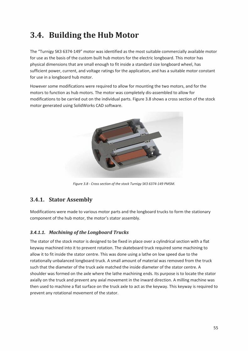
55
3.4. Building the Hub Motor
The “Turnigy SK3 6374-149” motor was identified as the most suitable commercially available motor for use as the basis of the custom built hub motors for the electric longboard. This motor has physical dimensions that are small enough to fit inside a standard size longboard wheel, has sufficient power, current, and voltage ratings for the application, and has a suitable motor constant for use in a longboard hub motor.
However some modifications were required to allow for mounting the two motors, and for the motors to function as hub motors. The motor was completely dis-assembled to allow for modifications to be carried out on the individual parts. Figure 3.8 shows a cross section of the stock motor generated using SolidWorks CAD software.
Figure 3.8 - Cross section of the stock Turnigy SK3 6374-149 PMSM.
3.4.1. Stator Assembly
Modifications were made to various motor parts and the longboard trucks to form the stationary component of the hub motor, the motor’s stator assembly.
3.4.1.1. Machining of the Longboard Trucks
The stator of the stock motor is designed to be fixed in place over a cylindrical section with a flat keyway machined into it to prevent rotation. The skateboard truck required some machining to allow it to fit inside the stator centre. This was done using a lathe on low speed due to the rotationally unbalanced longboard truck. A small amount of material was removed from the truck such that the diameter of the truck axle matched the inside diameter of the stator centre. A shoulder was formed on the axle where the lathe machining ends. Its purpose is to locate the stator axially on the truck and prevent any axial movement in the inward direction. A milling machine was then used to machine a flat surface on the truck axle to act as the keyway. This keyway is required to prevent any rotational movement of the stator.

56
3.4.1.2. Extension of the Longboard Trucks
The stator also needed a mechanical fixing to prevent axial movement in the outward direction. The stock motor uses an aluminium ‘core’ that extends right through the stator, allowing a circlip to be used to prevent axial movement. However the longboard truck reduces in diameter to an 8mm diameter axle inside the stator centre and therefore an adaptor was made to extend the larger diameter section of the truck axle so that it extends out the end of the stator centre. The adaptor was made by machining a piece of aluminium bar to match the cross section of the stator centre with an 8mm bore down the centre to allow it to fit over the longboard truck small diameter axle. The adaptor was cut to length and a slot was machined in the end to allow for a circlip to be inserted. The adaptor is fixed to the longboard truck using a high strength epoxy adhesive, “3M Scotch-Weld DP420”. Figure 3.9 shows a photograph of the modified longboard truck.
Figure 3.9 - The longboard truck after machining, extension of the aluminium axle, and location of the inside end bearing
mount.
3.4.1.3. Inside End Bearing Mount
The rotor must supported at both ends to withstand the radial loads seen in the hub motor application. Two small 8mm bore bearings support the rotor at the outside end, and a single 25mm bore bearing supports the rotor at the inside end. The two small bearings are mounted on the 8mm longboard truck axle without any modification. However, a mount for the large inside end bearing was required. This was done by cutting the large bearing mount off the stock motor ‘core’ and boring the centre out to match the diameter of the truck large diameter axle. This was fixed to the truck using the same high strength epoxy adhesive. The bearing mount was oriented with the shoulder on the inside edge to prevent the large bearing from experiencing any axial movement in the inward direction. This bearing mount has section cut out of it to allow for the stator wires to pass through in between the truck axle and the large bearing.
Figure 3.10 shows a photograph of the assembled longboard truck with the hub motor stator and inside end bearing support installed.

57
Figure 3.10 – Photograph of the modified longboard truck and stator assembly.
3.4.2. Rotor Assembly
Modifications were made to the rotor and longboard wheel to form the rotating assembly of the hub motor.
3.4.2.1. Removing the Motor Shaft.
The stock motor is constructed with an 8mm diameter centre shaft as part of the rotor. This hub motor application requires the shaft to be part of the stator assembly. Therefore the shaft was removed from the rotor using a press.
3.4.2.2. Machining the Rotor Outside End Bearing Housing
Removing the shaft from the rotor assembly also removed the means of support that the outside end bearings originally had. A new bearing support was created by machining a bearing housing into the rotor at the position where the shaft was originally attached. This bearing housing provides a press fit for the two small bearings to support the outside end of the rotor against the longboard truck 8mm diameter axle. When the wheel nut is in place, these small bearings provide radial support of the rotor and prevent axial movement in the outward direction.
3.4.2.3. Rotor Inside End Bearing Housing.
No modifications were required to the stock bearing housing for the inside end bearing. This bearing provides radial support of the rotor and the bearing housing is constructed with a shoulder that prevents axial movement of the rotor in the inward direction.
3.4.2.4. Longboard Wheel
The 90mm diameter longboard wheel required the centre to be bored out to a diameter that would allow the wheel to fit over the outside of the rotor. The polyurethane wheel was machined using a high speed router to cut through the material. The inside diameter of the wheel was machined out
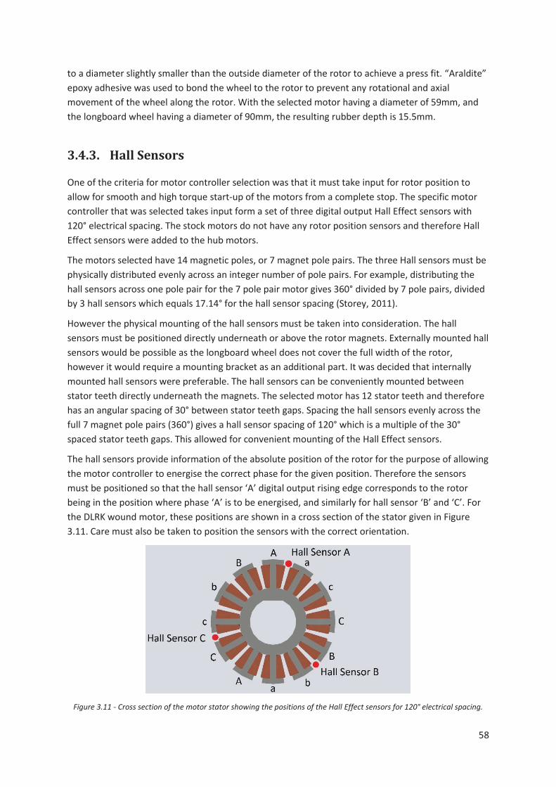
58
to a diameter slightly smaller than the outside diameter of the rotor to achieve a press fit. “Araldite” epoxy adhesive was used to bond the wheel to the rotor to prevent any rotational and axial movement of the wheel along the rotor. With the selected motor having a diameter of 59mm, and the longboard wheel having a diameter of 90mm, the resulting rubber depth is 15.5mm.
3.4.3. Hall Sensors
One of the criteria for motor controller selection was that it must take input for rotor position to allow for smooth and high torque start-up of the motors from a complete stop. The specific motor controller that was selected takes input form a set of three digital output Hall Effect sensors with 120° electrical spacing. The stock motors do not have any rotor position sensors and therefore Hall Effect sensors were added to the hub motors.
The motors selected have 14 magnetic poles, or 7 magnet pole pairs. The three Hall sensors must be physically distributed evenly across an integer number of pole pairs. For example, distributing the hall sensors across one pole pair for the 7 pole pair motor gives 360° divided by 7 pole pairs, divided by 3 hall sensors which equals 17.14° for the hall sensor spacing (Storey, 2011).
However the physical mounting of the hall sensors must be taken into consideration. The hall sensors must be positioned directly underneath or above the rotor magnets. Externally mounted hall sensors would be possible as the longboard wheel does not cover the full width of the rotor, however it would require a mounting bracket as an additional part. It was decided that internally mounted hall sensors were preferable. The hall sensors can be conveniently mounted between stator teeth directly underneath the magnets. The selected motor has 12 stator teeth and therefore has an angular spacing of 30° between stator teeth gaps. Spacing the hall sensors evenly across the full 7 magnet pole pairs (360°) gives a hall sensor spacing of 120° which is a multiple of the 30° spaced stator teeth gaps. This allowed for convenient mounting of the Hall Effect sensors.
The hall sensors provide information of the absolute position of the rotor for the purpose of allowing the motor controller to energise the correct phase for the given position. Therefore the sensors must be positioned so that the hall sensor ‘A’ digital output rising edge corresponds to the rotor being in the position where phase ‘A’ is to be energised, and similarly for hall sensor ‘B’ and ‘C’. For the DLRK wound motor, these positions are shown in a cross section of the stator given in Figure 3.11. Care must also be taken to position the sensors with the correct orientation.
Figure 3.11 - Cross section of the motor stator showing the positions of the Hall Effect sensors for 120° electrical spacing.
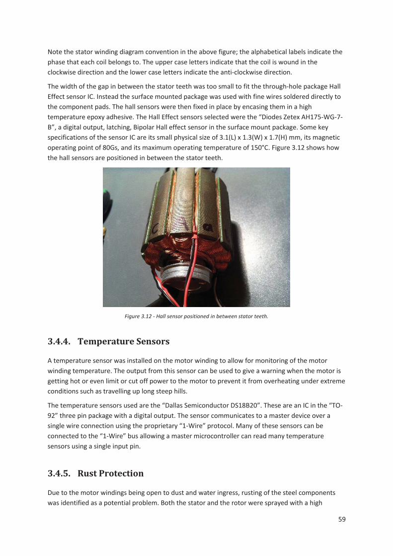
59
Note the stator winding diagram convention in the above figure; the alphabetical labels indicate the phase that each coil belongs to. The upper case letters indicate that the coil is wound in the clockwise direction and the lower case letters indicate the anti-clockwise direction.
The width of the gap in between the stator teeth was too small to fit the through-hole package Hall Effect sensor IC. Instead the surface mounted package was used with fine wires soldered directly to the component pads. The hall sensors were then fixed in place by encasing them in a high temperature epoxy adhesive. The Hall Effect sensors selected were the “Diodes Zetex AH175-WG-7-B”, a digital output, latching, Bipolar Hall effect sensor in the surface mount package. Some key specifications of the sensor IC are its small physical size of 3.1(L) x 1.3(W) x 1.7(H) mm, its magnetic operating point of 80Gs, and its maximum operating temperature of 150°C. Figure 3.12 shows how the hall sensors are positioned in between the stator teeth.
Figure 3.12 - Hall sensor positioned in between stator teeth.
3.4.4. Temperature Sensors
A temperature sensor was installed on the motor winding to allow for monitoring of the motor winding temperature. The output from this sensor can be used to give a warning when the motor is getting hot or even limit or cut off power to the motor to prevent it from overheating under extreme conditions such as travelling up long steep hills.
The temperature sensors used are the “Dallas Semiconductor DS18B20”. These are an IC in the “TO-92” three pin package with a digital output. The sensor communicates to a master device over a single wire connection using the proprietary “1-Wire” protocol. Many of these sensors can be connected to the “1-Wire” bus allowing a master microcontroller can read many temperature sensors using a single input pin.
3.4.5. Rust Protection
Due to the motor windings being open to dust and water ingress, rusting of the steel components was identified as a potential problem. Both the stator and the rotor were sprayed with a high

60
temperature motor winding lacquer to protect the stator core, rotor magnets, and rotor outer cylinder against corrosion.
3.4.6. Hub Motor Assembly.
Figure 3.13 shows all the individual parts of the left hand side hub motor assembly in exploded view along with the fully assembled right hand side hub motor.
Figure 3.13 - Exploded view of the electric longboard hub motor assembly.
To illustrate how all the individual parts are positioned within the assembly, Figure 3.14 shows a cross section along the axle of the hub motor.
Figure 3.14 - Cross section view of the electric longboard hub motor assembly.
Figure 3.15 show photographs of the actual dual hub motor assemblies installed on the electric skateboard prototype.

61
Figure 3.15 - Photograph of the actual electric skateboard hub motor assembly viewed from the underside (left) and the top side (right).
3.5. Electronics Enclosure
For reasons discussed previously, the decision was made to mount all of the electrical equipment in the underside of the longboard deck. A fibreglass enclosure was built which contains the battery pack, motor controllers, RC receiver, and all associated wiring.
3.5.1. Equipment Layout
The equipment was positioned with the battery pack located towards the front of the deck as an attempt to counter balance the added weight of the hub motors in the rear wheels. The motor controllers were located side by side at the back of the deck, near the motors. This allowed the motors to be connected directly to the motor controller without any extension of the motor phase wires.
3.5.2. Fibreglass Enclosure
Fibreglass was selected as the material for the enclosure due to it being a sufficiently strong and lightweight material, while giving the ability to mould the shape of the enclosure to that of the longboard deck. This particular deck is constructed of a bamboo plywood and fibreglass composite material. It is designed to flex under the weight of the rider in order to give certain desirable handling characteristics. A three dimensional fibreglass enclosure fixed to the underside of the deck would either need to be very strong and rigid to prevent the deck from any significant flex so that the fibreglass enclosure does not break, or be designed to flex with the deck. The latter was pursued so that it would not affect the handling characteristics of the deck.
This was achieved by building the enclosure with defined bend points. The top side of the enclosure (the side that is in contact with the underside of the deck) is constructed with a continuous plane of fibreglass. The underside and the edges of the enclosure are constructed as three discrete sections. The bend points are the two points between the three sections. The enclosure is fastened to the longboard deck using a metal clip at each side of the two bend points, and at each end using a strap.

62
The motor controllers require ventilation to allow for heat dissipation. The enclosure contains openings for the motor controller cooling fans exhaust air to exit the enclosure, and openings at each end for air to enter the enclosure. Figure 3.16 shows a photograph of the fibreglass electronics enclosure.
Figure 3.16 - Fibreglass enclosure for the electrical components of the electric longboard.
3.6. Complete Electric Skateboard Prototype
A photograph of the complete assembled electric skateboard prototype is shown in Figure 3.17. The total weight of the prototype is 8.6kg.
Figure 3.17 – Photograph of the complete electric longboard prototype.

63
4. Custom Built Motor Controllers
To allow for the testing of different motor control algorithms, a custom built motor controller was designed and constructed as part of this Masters project. The motor controller hardware was designed specifically to provide a platform on which multiple motor control techniques could be tested by simply flashing different motor control software onto the motor controller.
4.1. Hardware
The motor controller hardware was designed to be capable of running in either Six-Step ‘sensored’ control or FOC algorithms. The motor controller was designed to meet the specifications that would allow the electric longboard to meet the design objectives. Namely, each motor controller must be able to run with a 25.2V battery (six cell Lithium Polymer battery fully charged) and be capable of supplying 80A current as a burst rating. It was also desired for the motor controller to be small in size to allow for mounting two individual motor controllers side by side inside the fibreglass enclosure along with the battery pack, RC receiver, and all wiring.
4.1.1. Microcontroller
The computational requirements of FOC are relatively large compared to that of Six Step motor control algorithms. Therefore the microcontroller of choice must have sufficient processor speed and program memory to run the FOC algorithm. Other peripherals required include analogue inputs for current sampling, motor control timer which allows for ‘space vector modulation’, external interrupts and a hardware timer for hall sensor input, etc.
A microcontroller was selected that meets the requirements outlined above, the “STM32F303CCT6”. This specific microcontroller has additional peripherals to minimise the amount of external circuitry required for motor control applications. These include advanced motor control timers, programmable gain amplifiers, and comparators.
The programmable gain amplifiers can be used to amplify a small voltage differential signal across a shunt resistor for the purpose of current sensing and therefore removes the need for external op-amp ICs. The signal from the programmable gain amplifier is passed to the comparators which can be configured to trigger an ‘interrupt service routine’ for the purpose of over current protection. This again helps to minimise the number of components required in the motor controller.
Additionally, the STM32F303 contains a ‘Floating Point Unit’ coupled to the ARM Cortex-M4 processor which removes the burden of floating point operations from the CPU.
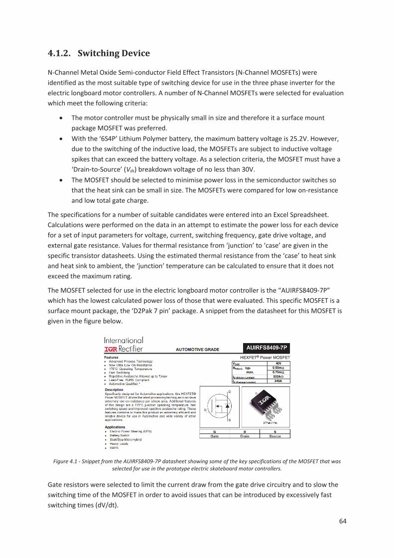
64
4.1.2. Switching Device
N-Channel Metal Oxide Semi-conductor Field Effect Transistors (N-Channel MOSFETs) were identified as the most suitable type of switching device for use in the three phase inverter for the electric longboard motor controllers. A number of N-Channel MOSFETs were selected for evaluation which meet the following criteria:
The motor controller must be physically small in size and therefore it a surface mount package MOSFET was preferred.
With the ‘6S4P’ Lithium Polymer battery, the maximum battery voltage is 25.2V. However, due to the switching of the inductive load, the MOSFETs are subject to inductive voltage spikes that can exceed the battery voltage. As a selection criteria, the MOSFET must have a ‘Drain-to-Source’ (Vds) breakdown voltage of no less than 30V.
The MOSFET should be selected to minimise power loss in the semiconductor switches so that the heat sink can be small in size. The MOSFETs were compared for low on-resistance and low total gate charge.
The specifications for a number of suitable candidates were entered into an Excel Spreadsheet. Calculations were performed on the data in an attempt to estimate the power loss for each device for a set of input parameters for voltage, current, switching frequency, gate drive voltage, and external gate resistance. Values for thermal resistance from ‘junction’ to ‘case’ are given in the specific transistor datasheets. Using the estimated thermal resistance from the ‘case’ to heat sink and heat sink to ambient, the ‘junction’ temperature can be calculated to ensure that it does not exceed the maximum rating.
The MOSFET selected for use in the electric longboard motor controller is the “AUIRFS8409-7P” which has the lowest calculated power loss of those that were evaluated. This specific MOSFET is a surface mount package, the ‘D2Pak 7 pin’ package. A snippet from the datasheet for this MOSFET is given in the figure below.
Figure 4.1 - Snippet from the AUIRFS8409-7P datasheet showing some of the key specifications of the MOSFET that was
selected for use in the prototype electric skateboard motor controllers.
Gate resistors were selected to limit the current draw from the gate drive circuitry and to slow the switching time of the MOSFET in order to avoid issues that can be introduced by excessively fast switching times (dV/dt).
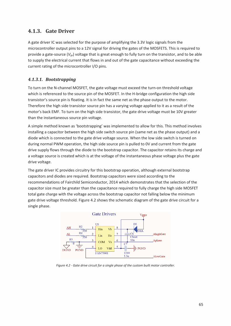
65
4.1.3. Gate Driver
A gate driver IC was selected for the purpose of amplifying the 3.3V logic signals from the microcontroller output pins to a 12V signal for driving the gates of the MOSFETS. This is required to provide a gate-source (Vgs) voltage that is great enough to fully turn on the transistor, and to be able to supply the electrical current that flows in and out of the gate capacitance without exceeding the current rating of the microcontroller I/O pins.
4.1.3.1. Bootstrapping
To turn on the N-channel MOSFET, the gate voltage must exceed the turn-on threshold voltage which is referenced to the source pin of the MOSFET. In the H-bridge configuration the high side transistor’s source pin is floating. It is in fact the same net as the phase output to the motor. Therefore the high side transistor source pin has a varying voltage applied to it as a result of the motor’s back EMF. To turn on the high side transistor, the gate drive voltage must be 10V greater than the instantaneous source pin voltage.
A simple method known as ‘bootstrapping’ was implemented to allow for this. This method involves installing a capacitor between the high side switch source pin (same net as the phase output) and a diode which is connected to the gate drive voltage source. When the low side switch is turned on during normal PWM operation, the high side source pin is pulled to 0V and current from the gate drive supply flows through the diode to the bootstrap capacitor. The capacitor retains its charge and a voltage source is created which is at the voltage of the instantaneous phase voltage plus the gate drive voltage.
The gate driver IC provides circuitry for this bootstrap operation, although external bootstrap capacitors and diodes are required. Bootstrap capacitors were sized according to the recommendations of Fairchild Semiconductor, 2014 which demonstrates that the selection of the capacitor size must be greater than the capacitance required to fully charge the high side MOSFET total gate charge with the voltage across the bootstrap capacitor not falling below the minimum gate drive voltage threshold. Figure 4.2 shows the schematic diagram of the gate drive circuit for a single phase.
Figure 4.2 - Gate drive circuit for a single phase of the custom built motor controller.

66
4.1.4. Current Sensing
Shunt resistors were used as the current sensing method for the motor controller. The small footprint of the current sensing resistors allows for mounting on the Printed Circuit Board (PCB) without adding a significant amount of area to the PCB footprint. The embedded op-amp and comparator peripherals in the selected STM32F303 microcontroller allow for simple implementation of shunt resistor current sensing without the need for additional circuitry.
For Field Oriented Control, current sensing on all three phases is required, and is implemented by placing the shunt resistors between the source pin of the low side MOSFETs and the power ground plane. The shunt resistors are sized according to the maximum current that is being measured. 3W surface mount metal strip resistors in the 6432 (metric) package with a resistance of 2mΩ were selected, using two in parallel to make up each of the three shunt resistor current sensors. At the maximum current rating of the motor (80A) this results in a voltage differential of 0.08V across the shunt resistors.
4.1.5. Power Supplies
With the electric skateboard battery voltage having a maximum voltage of 25.2V DC, power supplies are required to drop the voltage down to a level that is within the ratings of the other functional blocks that require a voltage source. Specifically, the gate drivers require a voltage in the range of 10 - 20V and the microcontroller requires a voltage in the range of 2.4 – 3.6V. A 12V power supply was designed for supplying the gate drivers and a 3.3V power supply was designed for supplying the microcontroller.
4.1.5.1. 12V Gate Drive Power Supply
An efficient switching voltage regulator was used for the 12V power supply so that minimal heat is generated in the power supply. This means that only a small area of PCB copper is required to act as a heat sink for the switching regulator IC. This power supply was designed according to the device manufacturer’s recommendations of inductor size, capacitor size, and feedback resistor network.
4.1.5.2. 3.3V Small Signal Power Supply
A linear voltage regulator was used for the 3.3V power supply. This power supply is fed from the 12V power supply so that the voltage drop across the regulator is not as great as if it were fed directly from the battery voltage. This is again to minimise the area of PCB copper required to act as the heat sink for the linear regulator IC.
4.1.6. DC Bus Capacitors
The DC bus capacitors (or DC link capacitors) play an important role in the inverter. In order to minimise the switching power loss in the semiconductor switches, the turn-on and turn-off times of the switches are designed to be fast. There is a significant inductive load on the inverter due to the

67
phase windings of the motor. This inductance opposes the change in current by creating an opposing voltage. Recall the equation for the voltage formed across an inductor with a changing current:
(4.1)
The rate of change of current can be very high and if no bus capacitance is present, the voltage spikes produced during the switch off of the semiconductor switches will also be very high. Now recall the equation for the current through a capacitor with a changing voltage: (4.2)
We can see that the voltage spikes from the inductive switching can be reduced by adding capacitors to absorb the energy from the voltage spikes. Note that the conduction path between the phase connections and the bus capacitors when the MOSFET is in the off-state is through the body diode of the high side switch.
Additionally, when the MOSFET is switched on, the bus capacitors provide a low impedance (due to the close proximity) voltage source for energising the phase winding when the semiconductor switch is turned on.
The amount of ripple current, Irip that the bus capacitors are subject to can be calculated for a specific PWM duty cycle, D with given bus voltage Vbus, switching frequency f, and phase inductance L. The following equation is mathematically proven in reference Salcone & Bond, 2009. (4.3)
This relationship is best illustrated by plotting the resulting ripple current against duty cycles from 0 - 100%. Figure 4.3 shows the calculated values for ripple current over the full range of duty cycles for a bus voltage of 22.2V, a switching frequency of 20kHz, and a load with an inductance of 50μH. We can clearly see that the ripple current is greatest for a duty cycle of 50%.
Figure 4.3 - Plot illustrating the relationship between ripple current through the bus capacitors and with varying duty cycle
for the electric skateboard motor controller.
0
1
2
3
4
5
6
0 0.2 0.4 0.6 0.8 1
Ripp
le C
urre
nt [A
]
Duty Cycle
Ripple Current vs Duty Cycle
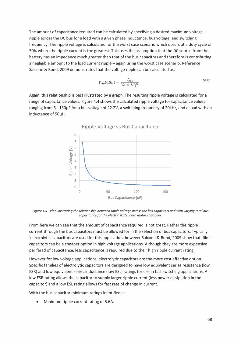
68
The amount of capacitance required can be calculated by specifying a desired maximum voltage ripple across the DC bus for a load with a given phase inductance, bus voltage, and switching frequency. The ripple voltage is calculated for the worst case scenario which occurs at a duty cycle of 50% where the ripple current is the greatest. This uses the assumption that the DC source from the battery has an impedance much greater than that of the bus capacitors and therefore is contributing a negligible amount to the load current ripple – again using the worst case scenario. Reference Salcone & Bond, 2009 demonstrates that the voltage ripple can be calculated as: (4.4)
Again, this relationship is best illustrated by a graph. The resulting ripple voltage is calculated for a range of capacitance values. Figure 4.4 shows the calculated ripple voltage for capacitance values ranging from 5 - 150μF for a bus voltage of 22.2V, a switching frequency of 20kHz, and a load with an inductance of 50μH.
Figure 4.4 - Plot illustrating the relationship between ripple voltage across the bus capacitors and with varying total bus
capacitance for the electric skateboard motor controller.
From here we can see that the amount of capacitance required is not great. Rather the ripple current through the bus capacitors must be allowed for in the selection of bus capacitors. Typically ‘electrolytic’ capacitors are used for this application, however Salcone & Bond, 2009 show that ‘film’ capacitors can be a cheaper option in high voltage applications. Although they are more expensive per farad of capacitance, less capacitance is required due to their high ripple current rating.
However for low voltage applications, electrolytic capacitors are the more cost effective option. Specific families of electrolytic capacitors are designed to have low equivalent series resistance (low ESR) and low equivalent series inductance (low ESL) ratings for use in fast switching applications. A low ESR rating allows the capacitor to supply larger ripple current (less power dissipation in the capacitor) and a low ESL rating allows for fast rate of change in current.
With the bus capacitor minimum ratings identified as:
Minimum ripple current rating of 5.6A.
0
1
2
3
4
5
6
7
8
0 50 100 150
Ripp
le V
olta
ge [V
]
Bus Capacitance [uF]
Ripple Voltage vs Bus Capacitance

69
Minimum capacitance of 40uF, allowing for a ripple voltage of 5% of the nominal supply voltage.
Two capacitors connected in parallel were selected for this purpose: Rubycon ZLJ series, 50V, 820uF, 3370mA Aluminium Electrolytic capacitors.
4.1.7. Heat Sink
As discussed in section 2.2.5.2, the semiconductor switches in the three phase inverter dissipate power in the form of heat due to resistive and switching power loss. The worst case total power dissipation for the six semiconductor switches was calculated in section 3.3.3 to be 40W. However the motor controllers were not designed to run at their maximum rating continuously nor are they likely to be required in their designed application in the electric skateboard. A typical use of the electric skateboard would see a high amount of current while accelerating then a lower continuous current while travelling at a constant speed.
The thermal capacity of the heat sink allows for bursts of high power where the heat is absorbed by the heat sink. This heat is continuously dissipated by forced convection (due to the air speed past the moving skateboard) from the heat sink to the atmosphere.
Using Texas Instruments Application Note on heat sinks as a guide (Texas Instruments, 2011), the heat sink requirements were calculated as: (4.5)
Using maximum junction temperature, TJ = 150°C
Ambient temperature, TA = 20°C
Heat being dissipated, PD = 40W
Thermal resistance from MOSFET junction to case, θJC = 0.4°C/W
Thermal resistance from MOSFET case to heat sink (thermal interface material), θCS = 0.9°C/W
We get thermal resistance from heat sink to atmosphere, θSA must be less than 1.95°C/W
A suitable heat sink was identified. The heat sink has dimensions 43mm (l) x 43mm (w) x 8mm (h) and thermal resistance of 3.2°C/W with air flow >5m/s (minimal electric skateboarding speed). Two of these heat sinks are to be used for each motor controller to get the thermal resistance below the calculated minimum.
4.1.8. Hall Sensor Interface
The Hall Effect sensors have ‘open collector’ digital outputs. This means that for a logical low output the output pin is pulled to the sensors GND reference, and for a logic high output the output pin is left floating. For the microcontroller to be able to read the high level logic output, the signal must have weak pull up resistors to pull the output signal to a suitable high logic level when the hall

70
sensor output is in the floating output state. These pull up resistors are included in the PCB hall sensor interface.
When the hall sensors are installed inside the motor, the output signals are subject to high levels of electrical noise. Low pass filters are included in the hall sensor interface circuitry in an attempt to reduce this noise as to reduce the risk causing false readings of the rotor position.
Each of the three hall sensor signals are routed to separate pins of the microcontroller. The pins used for these inputs are ones that are able to be used as external interrupts. This means that the microcontroller does not need to continuously poll the input pins at a high frequency to update the rotor position reading. Instead whenever the input changes logic level, an interrupt is generated to update the rotor position reading.
4.1.9. Throttle Input
A three pin header was included on the control PCB. This header provides a 3.3V power source for powering an external RC receiver. The third pin is connected to a digital input pin of the microcontroller that is able to be ported to a timer peripheral to be used in input capture mode. This allows the user throttle input to be a RC car pistol type wireless transmitter.
The receiver for the RC transmitter outputs a PWM signal whose duty cycle represents the throttle position from the user. This is a 50Hz cycle where the full brake signal is represented as a 1000us pulse width, and the full throttle signal is represented as a 2000us pulse width.
4.1.10. Analogue Debug Outputs
The STM32F303 microcontroller has a built in two channel Digital to Analogue Converter (DAC) peripheral. The output pins for the two channels are wired to test points on the control PCB. These analogue outputs are useful in the debugging and testing of the motor controllers. They can be set to represent analogue values within the control software in real time and their waveforms viewed using an oscilloscope.
4.1.11. Communication Ports
A header port is included to allow easy access to the microcontrollers Serial Wire Debug (SWD) port. This is the port used for flashing firmware to the microcontroller and to perform software debugging sessions. A computer communicates to the microcontroller through this port via a ST Link tool (an external circuit board to convert between USB and SWD communications).
A second communications port allows for Universal Synchronous Asynchronous Receiver Transmitter (USART) communications. This port is useful in providing serial communications to a computer which can be used for either control or monitoring of the motor controller.

71
4.1.12. Component Layout
A Printed Circuit Board (PCB) design was created using Altium Designer software and professionally printed for the custom built motor controllers. The PCB design uses two separate boards which are stacked on top of one another. All of the power electronics of the inverter and associated components allocated to one board, referred to as the “power PCB”. All other components are allocated to the second board, referred to as the “control PCB”. This scheme has numerous advantages over a single PCB design. The overall footprint of the motor controller is reduced in size. It allows for separation of the small signal control electronics from the power electronics. It also allows for future customisation if a motor controller with different voltage and current ratings is desired; only a new power PCB is required as the control PCB can be used as a “universal” control board.
In general terms, the individual components are grouped into functional blocks. For example, all components associated with the 12V switching regulator power supply are physically positioned in a cluster with close proximity to one another. The cluster is then strategically positioned near the other functional which require input from and/or output to the power supply.
The PCBs are sized to be large enough for the components that are designated to each PCB. Additionally, the width of the PCB was dictated by the width of the heat sink. It was desirable to arrange the power MOSFETs so that they are spread evenly across the heat sink therefore the width of the PCB was selected to allow for this. A two layer PCB was selected and components were allowed to be positioned on both sides of the PCB. See Appendix C for the Altium Designer schematic diagrams and PCB design.
4.1.12.1. Power PCB
The power PCB is made up of the semiconductor switches and associated components which make up the three phase inverter. This includes the power MOSFETs, gate resistor networks, shunt resistor current sensors, bus capacitors, power connections for the battery and motor, and header pins for the interface with the control PCB.
A major concern with using surface mount components for the power electronics was the ability to remove heat from the components. The D2-Pak MOSFETs have the tab as the ‘drain’ pin which is soldered directly to the copper on the PCB. The majority of heat is conducted through this interface therefore a large amount of heat is transferred to the PCB traces. The layout was designed around optimising heat removal from the MOSFETs through these PCB traces. The drain pins of the high side switches have a common net, Vbatt which is connected to the positive terminal of the battery pack. The low side switch drain pins have a separate net for each of the three phases. These nets are the phase outputs of the inverter and are connected to the motor terminals. This gives four nets which conduct heat directly to PCB traces from the MOSFETs.
All six MOSFETS are positioned on the top side of the PCB and a heat sink is positioned directly below. The four nets that require heat removal are brought through from the top layer to the bottom layer of the PCB through an array of ‘vias’ for each MOSFET. As the Vbatt net is the primary means of heat removal for all three high side MOSFETs, it is allocated half of the area of the heat sink. A ‘power plane’ for this net is positioned directly below the high side switches for maximum heat transfer from the MOSFET drain pin through to the bottom layer then to the heat sink.

72
The remaining three nets are the primary means of heat removal for each of the three low side switches and therefore are allocated one sixth of the heat sink area each. A power plane for each net is positioned directly below each of the low side switches. The three nets are brought through from the top layer to the bottom layer through an array of vias to conduct heat from the MOSFETs.
A thermal interface material is placed between the heat sink and the PCB. This provides the function of electrically isolating the power planes from the heat sink to avoid creating short circuits through the aluminium heat sink material. The thermal interface material also helps to increase the contact area between the PCB and heat sink as it is a flexible material which moulds to the shape of the surfaces to fill in small imperfections in the surfaces.
A second heat sink is placed on top of the MOSFET cases to allow for heat removal through the MOSFET bodies. A thermal interface material is placed in between for the purpose of increasing the contact area. Minor differences in MOSFET height can cause some of the MOSFETs to not have proper contact with the heat sink. The thermal interface material helps to minimise this issue. The two heat sinks are held in place with two M3 bolts between them, through the PCB. The MOSFETs and PCB are effectively clamped between the two heat sinks.
Figure 4.5 shows how the functional blocks are arranged on the power PCB.
Figure 4.5 - Functional block layout of the Power PCB top side (left) and bottom side (right).
Each of the six gate resistor networks are placed as close as possible to the corresponding MOSFET gate pins. The shunt resistors are placed directly in line with and in close proximity to the low side switch ‘source pins’. These resistors then connect to the power ground plane on the top side of the power PCB. The bus capacitors are positioned such that they are outside of the area covered by the heat sinks while still being in as close proximity as possible to the MOSFETs.
Custom made footprints were used for soldering power carrying wires directly to the top side of the PCB in a surface mount style to keep the bottom layer free of any protrusions. This leaves an empty surface on the bottom side for the heat sink to sit flat against the PCB’s heat conducting power planes. The MOSFETs were spaced a sufficient distance apart to allow for the phase wires to pass in between, and underneath the top side heat sink.

73
A photograph of the assembled power PCB is given in Figure 4.6.
Figure 4.6 - Photograph of the assembled power PCB.
4.1.12.2. Control PCB
The control PCB is made up of the remaining components required for the motor controller. Namely the microcontroller, power supplies, gate drivers, and all associated discrete components. The dimensions of this PCB were selected to allow for the control board to fit in the area above the power PCB, between the top side heat sink and the edge of the board. Figure 4.7 shows how the functional blocks are arranged on the control PCB.
Figure 4.7 - Functional block layout of the Control PCB top side (left) and bottom side (right).
The layout of the control PCB places functional blocks in logical order for the interconnections between one another. A power plane was placed on the bottom layer of the control PCB connected to the “power ground” net. This plane was extended to cover some of the top layer over the area occupied by the linear regulator power supply for heat sinking purposes. A second power plane was placed over the remaining area on the top layer of the PCB connected to the “digital Ground” net.
The electrical connections (traces) between functional blocks are generally routed with vertical running traces on the top layer of the PCB and horizontal running traces on the bottom layer. This helped to minimise the number of times that a trace needed to jump between layers to get to its destination. If no such systematic approach is taken, the final traces may end up needing to jump

74
between layers many times to reach their destination. With this approach, a single trace should need to jump between layers no more than a few times. Photographs of the assembled control PCB top and bottom sides are given in Figure 4.8 below.
Figure 4.8 - Photograph of the assembled control PCB top side (left) and bottom side (right).
4.1.13. Complete Motor Controller Hardware
Finally, Figure 4.9 shows the complete assembled motor controller hardware with heat sinks installed.
Figure 4.9 - Photograph of the complete motor controller hardware.
4.2. Software
Software for the custom built motor controllers was developed using “IAR Embedded Workbench”. This Integrated Development Environment (IDE) was selected due to its compatibility with the microcontroller that are used in the motor controller hardware. Additionally the manufacturer of the microcontroller, ST Microelectronics provides an open source code library for its “STM32” microcontroller range. This library is able to be utilised in the “IAR Embedded Workbench” IDE.
The ST Microelectronics code library provides drivers for the microcontroller’s peripherals. This greatly simplifies the implementation of code that utilises various peripherals such as timers, counters, analogue to digital converters, etc. The programmer need not access the specific control
75
registers for peripherals directly. Instead the programmer may work at a higher level of abstraction from the device hardware and the peripheral drivers are used to make the connection between high level programs and the low level control registers.
Among other microcontroller manufacturers, ST Microelectronics also provide a motor control library specifically for the purpose of reducing the time required for developing software for motor control. This motor control library includes functions used in the implementation of FOC. The motor control library is provided as complied source code which means that the programmer is able to use the included functions as they are but it is not possible to modify that code. Using this freely available software library package greatly reduced the complexity of creating firmware packages that allow the motor controllers to drive the motor under Six-Step Control or FOC. Source code for both the Six-Step Control and FOC firmware main functions is provided in Appendix D.
4.2.1. Six-Step Control
Code was written for a firmware package that can be flashed to the microcontroller that drives the motor under the Six-step control technique. Refer back to Section 2.3.3 to recap on the theory of Six-step control. The standard peripheral driver library and the ‘Six-Step’ motor control library was used in developing this software.
4.2.1.1. Initialisation
When power is first applied to the microcontroller, it executes a block of code which initialises (configures) all of the microcontroller peripherals which are used in the specific application. This code is executed once only each time the microcontroller starts up. In the Six-Step Control firmware, the initialisation code is used to configure the following peripherals.
Timer 1 (TIM1) is an advanced 16bit timer and was used as the motor control timer with clock frequency of 64MHz and pre-scalar value of zero. A reset value of 62335 (which is calculated as: 216 – 1 – 3200) gives a PWM frequency of 20kHz with the output adjustable to a resolution of 3200 increments. The advanced timer was configured as three complementary channels in PWM output mode with 700ns (counter value of 45) software inserted dead time. TIM1 also has a commutation feature which was utilised for the Six-step control firmware. This feature allows the configuration of the timer for the next step of the six step sequence to be set in advance. When the commutation event occurs, the configuration of all channels are changed at the same time in one instruction. The commutation event is generated directly from the hall sensor input timer.
TIM1 Channel 1 output (phase A high side gate driver signal) is mapped to pin A8. TIM1 Channel 1 N output (phase A low side gate driver signal) is mapped to pin B13. TIM1 Channel 2 output (phase B high side gate driver signal) is mapped to pin A9. TIM1 Channel 2 N output (phase B low side gate driver signal) is mapped to pin B14. TIM1 Channel 3 output (phase C high side gate driver signal) is mapped to pin A10. TIM1 Channel 3 N output (phase C low side gate driver signal) is mapped to pin B15.
Timer 4 (TIM4) is a general purpose 16bit timer and was used as the Hall sensor input timer. TIM4 was configured to run on a clock frequency of 32MHz with pre-scalar value of 16 resulting in a counter frequency of 2MHz. TIM4 runs in input capture mode. The three hall sensor inputs are

76
evaluated using the “exclusive or” (XOR) operator so that the output toggles each time one of the sensor inputs change state. This output toggle triggers the timer counter value to be read and used for the speed calculation and then cleared back to zero and the timer restarted. The minimum speed that is able to be measured without timer overflows is 0.73 revolutions per second.
TIM4 channel 1 as input capture and mapped to pin B6 (Hall A input). TIM4 channel 2 as input capture and mapped to pin B7 (Hall B input). TIM4 channel 3 as input capture and mapped to pin B8 (Hall C input).
Timer 16 (TIM16) is a general purpose 16bit timer and was used as the RC Receiver PWM input timer. TIM16 was configured to run on a clock frequency of 32MHz with pre-scalar value of 2 resulting in a counter frequency of 16MHz. TIM16 is configured to run in input capture mode. This timer is able to time the 1 – 2ms input pulse from the RC receiver to a resolution of 16,000 increments.
TIM16 channel 1 as input capture and mapped to pin B4.
Timer 3 (TIM3) is a 16bit general purpose timer and was used as the user time base timer for scheduling events. TIM3 shares the same clock source as TIM4 (32MHz) and was configured to run on a pre-scalar of 2, resulting in a counter frequency of 16MHz. This timer was set to generate an interrupt at 2kHz using a reload value of 57535 (calculated as: 216 – 1 – 8000). This was selected as the frequency for executing high frequency tasks. Medium and low frequency tasks occur at a multiple of this time period.
TIM3 set as an internal timer not mapped to any pins.
Operational Amplifier (OPAMP) 1 and 2 as phase current feedback programmable gain amplifiers with a gain of 16. Note that there are two OPAMPs which are shared between the current sensors of the three phases based on the current step of the Six-step sequence.
Channel 1 non-inverting input (phase A shunt resistor input) is mapped to pin A1. Channel 2 non-inverting input (phase B shunt resistor input) is mapped to pin A7. Channel 3 non-inverting input (phase C shunt resistor input) is mapped to pin B0. OPAMP 1 output is mapped to pin A2. OPAMP 2 output is mapped to pin A6.
ADC1 and ADC2 are 12bit ADCs and are configured as current sensing analogue inputs from the OPAMP outputs. Analogue watchdogs were set up to trigger an interrupt if the ADC readings exceeds 4012 which corresponds to a current of 130A.
ADC1 channel 3 input is mapped to pin A2 (OPAMP 1 output). ADC2 channel 3 input is mapped to pin A6 (OPAMP 2 output).
ADC3 is a 12bit ADC and is configured as the heat sink temperature sensor analogue input. An analogue watchdog was set up to trigger an interrupt if the ADC reading exceeds 1241 which corresponds to a temperature of 60°C.
ADC3 channel 1 input is mapped to pin B1.
ADC4 is a 12bit ADC and is configured as the voltage sensing analogue input. An analogue watchdog was set up to trigger an interrupt if the ADC reading exceeds 3289 which corresponds to a voltage of 35V.

77
ADC4 channel 3 is mapped to pin B12.
The DAC was configured as a user analogue output:
DAC channel 1 is mapped to pin A4. DAC channel 2 is mapped to pin A5.
The USART was configured as a communications port:
USART3 TX mapped to pin B10. USART3 RX mapped to pin B11.
The SWD was configured as a communications port:
SWDIO mapped to pin A13. SWCLK mapped to pin A14.
External interrupts:
Hall sensor input pins are configured to trigger an interrupt on both rising and falling edges to generate commutation events and interface with TIM4.
Throttle input pin is configured to trigger an interrupt on both rising and falling edges to interface with TIM16.
Internal Interrupts:
TIM1 is configured to trigger an interrupt on both overflow and when the timer reaches the PWM output capture and compare register.
TIM3 is configured to trigger an interrupt when the timer reaches the user time base capture and compare register.
ADC1, ADC2, ADC3, and ADC4 are configured to trigger an interrupt on end of conversion and when readings exceed a specified value (analogue watchdog).
The initialisation code is generated using software by ST Microelectronics called “STM32CubeMX”. A snippet of the pin-out configuration is shown in Figure 4.10.

78
Figure 4.10 - Pin-out graphic generated by "STM32CubeMX" software.
The “STM32CubeMX” software also provides a graphical display of the system and peripheral clock configuration, as provided in Figure 4.11.
Figure 4.11 – Clock configuration graphic generated by "STM32CubeMX" software.

79
4.2.1.2. Main Routine
The main loop is used for executing tasks which are not time critical. Three categories of tasks were created which are executed at different frequencies. High frequency tasks are executed at 2kHz, medium frequency tasks are executed at 500Hz, and low frequency tasks are executed at 50Hz.
High frequency tasks include the following sub-routines:
Apply low pass filter for motor current. Apply limits for current. Update DAC outputs.
Medium frequency tasks include the following sub-routines:
Update battery voltage and apply limits.
Low frequency tasks include the following sub-routines:
Apply low pass filter to throttle input. Update temperatures and apply limits.
4.2.1.3. Interrupt Routines
Interrupt routines are used for executing time critical tasks. Two internal interrupts and two external interrupts are used in the Six-Step Control firmware. These interrupts are configured in the “initialise” block of code and execute a wet of instructions when triggered by either their corresponding internal trigger or external trigger respectively. These interrupt routines execute the following functions:
Timer 1 overflow interrupt:
Turn the high side PWM output pin off. After a dead-time delay of 700ns, turn the low side PWM output pin on. Reload the timer with the predefined auto-reload value of 62335 to achieve a 20kHz PWM
frequency.
Timer 1 capture/compare interrupt:
Turn the low side PWM output pin off After a dead-time delay of 700ns, turn the high side PWM output pin on. Trigger an analogue to digital conversion to measure the phase current.
Timer 3 capture/compare interrupt:
User time-base update for task scheduling.
Analogue to Digital converters end of conversion interrupt:
Update the corresponding variable.
Timer 4 external interrupt:
Commutate motor. Calculate speed. Increment tachometer pulse count.

80
Timer 16 External interrupt:
Update throttle variable. Update PWM duty cycle.
4.2.2. FOC
Code was written for a firmware package that can be flashed to the microcontroller that drives the motors under the FOC technique. Refer back to Section 2.3.4 to recap on the theory of FOC.
As mentioned previously, the ST Microelectronics FOC motor control library was utilised for the implementation of FOC along with the standard peripheral driver library. This allowed for the FOC firmware to be written at an application level. The implementation uses the exact same hardware as used in the Six-step Control firmware and therefore the microcontroller pin-out remains the same. In fact, much of the initialisation code is the same for configuring the peripherals used in the FOC implementation.
4.2.2.1. Initialisation
Timer 1 (TIM1) advanced 16bit timer was used as the motor control timer with frequency clock frequency of 64MHz and pre-scalar value of zero. For SVM, the motor control timer is configured to run as centre aligned PWM output. In this mode, the timer counts up until it reaches the overflow value, then counts down until it reaches the auto-reload value. As the timer reaches the capture-compare value when counting upwards, the PWM output pin is turned on. As the timer reaches the capture-compare value when counting downwards, the PWM output pin is turned off. There are three capture-compare registers used, one for each of the three phases of the inverter. This way, all three phases are controller using the one timer.
A reset value of 63935 (which is calculated as: 216 – 1 – 1600) gives a PWM frequency of 20kHz with the output adjustable to a resolution of 1600 increments. The advanced timer was configured as three complementary channels in centre aligned PWM output mode with 700ns (counter value of 45) software inserted dead time:
TIM1 Channel 1 output (phase A high side gate driver signal) is mapped to pin A8. TIM1 Channel 1 N output (phase A low side gate driver signal) is mapped to pin B13. TIM1 Channel 2 output (phase B high side gate driver signal) is mapped to pin A9. TIM1 Channel 2 N output (phase B low side gate driver signal) is mapped to pin B14. TIM1 Channel 3 output (phase C high side gate driver signal) is mapped to pin A10. TIM1 Channel 3 N output (phase C low side gate driver signal) is mapped to pin B15.
Timer 4 (TIM4) general purpose 16bit timer was used as the Hall sensor input timer. TIM4 was configured identically to that of the Six-Step Control implementation.
Timer 16 (TIM16 general purpose 16bit timer was used as the RC Receiver PWM input timer. Tim16 was configured identically to that of the Six-Step Control implementation.
Timer 3 (TIM3) 16bit general purpose timer was used as the user time base timer for scheduling events. TIM3 was configured identically to that of the Six-Step Control implementation.
81
Operational Amplifier (OPAMP) 1 and 2 were configures as phase current feedback programmable gain amplifiers with gain of 16. OPAMP2 and OPAMP2 were configured identically to that of the Six-Step Control implementation.
ADC1 and ADC2 12bit ADCs were configured as current sensing analogue inputs from the OPAMP outputs. This configuration was identical to that of the Six-Step Control implementation.
ADC3 12bit ADC was configured as the heat sink temperature sensor analogue input. This configuration was identical to that of the Six-Step Control implementation.
ADC4 12bit ADC was configured as the voltage sensing analogue input, identical to that of the Six-Step Control implementation.
The DAC was configured as a user analogue output, identical to that of the Six-Step Control implementation.
The USART communications port was configured identically to that of the Six-Step Control implementation.
The SWD communications port was configured identically to that of the Six-Step Control implementation.
The external interrupts were configured identically to that of the Six-Step Control implementation.
The Internal Interrupts were configured identically to that of the Six-Step Control implementation.
4.2.2.2. Main Routine
Again, the main loop is used for executing tasks which are not time critical. The main loop was utilised for executing three categories of tasks. High frequency tasks are executed at 2kHz, medium frequency tasks are executed at 500Hz, and low frequency tasks are executed at 50Hz.
High frequency tasks include the following sub-routines:
Apply low pass filter for motor current. Apply limits for current. Update DAC outputs. Send and receive serial data for interfacing with the PC based monitoring tool. Run the motor control application finite state machine.
Medium frequency tasks include the following sub-routines:
Update battery voltage and apply limits.
Low frequency tasks include the following sub-routines:
Apply low pass filter to throttle input. Update temperatures and apply limits.
4.2.2.3. Interrupt Routines
Interrupts are used for executing time critical tasks. Two internal interrupts and two external interrupts are used in the FOC firmware. These interrupt routines execute the following functions:

82
Timer 1 overflow interrupt:
Adjust the timer to count downwards for the implementation of centre aligned PWM. Trigger analogue to digital conversions to measure phase currents.
Timer 1 auto-reload interrupt:
Adjust the timer to count upwards for the implementation of centre aligned PWM. Calculate the estimated rotor position based on hall sensor input extrapolation. Perform Clarke transformation of variables to calculate Iα and Iβ in the Alpha-Beta reference
frame. Perform Park transformation of variables to calculate Id and Iq in the Direct-Quadrature
reference frame. Calculate Vd and Vq output voltages using the direct axis and quadrature axis PID controllers
based on the measured Id and Iq values and the Id and Iq set-points. Perform the reverse Park transformation of variables to calculate Vα and Vβ for the SVM
module.
Timer 1 capture/compare interrupt:
If the timer is counting upwards, turn the low side PWM output pin off and after a delay of 700ns, turn the high side PWM output pin on.
If the timer is counting downwards, turn the high side PWM output pin off and after a delay of 700us, turn the low side PWM output pin on.
Timer 3 capture/compare interrupt:
User time-base update for task scheduling.
Analogue to Digital converters end of conversion interrupt:
Update the corresponding variable.
Timer 4 external interrupt:
Transfer to the next sector of the SVM scheme. Calculate speed. Increment tachometer pulse count.
Timer 16 External interrupt:
Update throttle variable.

83
5. Results
With the custom built motor controller hardware assembled, the microcontrollers were able to be flashed with the custom written firmware. The firmware for Six-step motor control was flashed to the motor controller and its performance evaluated. Similarly, the firmware for FOC was flashed to the motor controller and its performance evaluated. This allowed for conclusions to be drawn about the relative performance of the two motor control techniques.
5.1. Bench Testing
Testing of the two control techniques was first performed in bench testing a using purpose built test rig. This allowed for rigorous testing of the motor controllers driving a PMSM under load for both Six-step and FOC motor control techniques.
5.1.1. Test Rig
It was desired to construct a test rig that would allow for testing of the motor controllers under load conditions in order to best resemble the real world application. Ideally, the motor controllers would be able to be tested to the maximum load that they would be subjected to when used in the electric skateboard application. This was identified in section 3.2.2 as 3440W input power (22.2V at 155A). This corresponds to a speed of 311 rad.s-1 (2970 RPM) and mechanical load of 9.58Nm which is a 2980W mechanical load. This load is shared between two electric motors therefore the test rig was designed to allow for testing of up to 1500W mechanical load.
Clearly this is a significant mechanical load and difficult to dissipate. A mechanical disk brake setup would need to be large otherwise it would quickly overheat. A fan or propeller setup would be dangerous and would need to be caged and the tests conducted outdoors.
Perhaps then it would be easier to convert the mechanical load to an electrical load. A three phase PMSM acting as a generator provides a three phase electrical AC voltage at the winding terminals. Using the same motors and that were selected for use in the prototype electric skateboard, the generating motor would produce approximately 1275W (assuming an efficiency of 0.85) which is around 22.2V at 57A rectified DC. Again this is difficult load to dissipate. A large resistor bank or similar could be used to dissipate this electrical load as heat.
Alternatively and more conveniently, rectified DC electrical power can be returned to the motor controller which is powering the driving motor. Under this scheme, the re-generated energy is circulated back to the driving motor. There is no need for a means of dissipating the energy as heat. Although this might sound like a complicated solution, it is actually quite simple. A second identical motor controller has already been built due to the electric skateboard prototype requirement of one motor controller for each of the two motors. The motor controller software has been written to include a regenerative braking function.
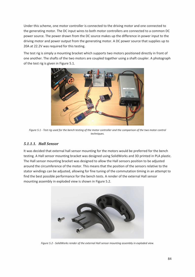
84
Under this scheme, one motor controller is connected to the driving motor and one connected to the generating motor. The DC input wires to both motor controllers are connected to a common DC power source. The power drawn from the DC source makes up the difference in power input to the driving motor and power output from the generating motor. A DC power source that supplies up to 20A at 22.2V was required for this testing.
The test rig is simply a mounting bracket which supports two motors positioned directly in front of one another. The shafts of the two motors are coupled together using a shaft coupler. A photograph of the test rig is given in Figure 5.1.
Figure 5.1 - Test rig used for the bench testing of the motor controller and the comparison of the two motor control
techniques.
5.1.1.1. Hall Sensor
It was decided that external hall sensor mounting for the motors would be preferred for the bench testing. A Hall sensor mounting bracket was designed using SolidWorks and 3D printed in PLA plastic. The Hall sensor mounting bracket was designed to allow the Hall sensors position to be adjusted around the circumference of the motor. This means that the position of the sensors relative to the stator windings can be adjusted, allowing for fine tuning of the commutation timing in an attempt to find the best possible performance for the bench tests. A render of the external Hall sensor mounting assembly in exploded view is shown in Figure 5.2.
Figure 5.2 - SolidWorks render of the external Hall sensor mounting assembly in exploded view.

85
5.1.1.2. Power Monitoring
In an ideal test rig we would be able to measure the input electrical power as well as output speed and torque from the motor under test. The output speed, torque, and their product, mechanical power would be useful in the analysis of the performance of the two control techniques. Unfortunately the torque measurement is difficult to obtain. A complicated test rig would be required which is able to measure the force acting on one of the motors using a load cell, strain gauge, or equivalent, and the distance from the motors axis of rotation would be used to calculate the load torque. It was desired that the performance would be evaluated over the full speed range therefore the torque measurement would need to be time synchronised to the speed and electrical power measurements.
For this bench testing, a simplified approach has been taken. The electrical voltage, current, and power is measured at the input of the driving motor controller and also at the output of the generating motor controller. The generating motor controller configuration was kept the same for the testing of both control techniques in that it was using FOC in regenerative braking mode. This way the load can be considered to be the same for both tests and the power losses in the generating motor and controller at a given speed can be considered to be the same. This allowed for comparative performance measurements to be taken.
A power monitoring device with data logging functionality was used for these tests. The logging frequency was set to the highest that the device would allow which is 4 samples per second. The power meter is connected in series in between the motor controller under test and the power supply. It records the following measurements:
Supply voltage [V] Supply current [A] Supply power [W] Capacity used [mAh] Internal temperature [°C] Three external temperatures from digital temperature sensors using the Dallas “1-Wire”
communications protocol [°C] Pulse input period [μs] Pulse input on time [μs]
The signal from one of the rotor position Hall sensors is connected to the pulse input pin to allow for the speed measurements to be obtained. The pulse period is related to speed of the electric skateboard prototype using the formula given in equation (5.3).
(5.1)
(5.2)
(5.3)

86
5.1.2. Test Setup
For a fair comparison between the two control techniques, a test load is required which must be identical for both the Six-Step Control and FOC tests. The motor controller of the generating motor is able to vary the amount of current that is being regenerated and hence is able to vary the load torque. This motor was set to run in regenerative braking mode under FOC using ST Microelectronics Motor Control Library. This library provides an instruction to set a load current (motor phase current). This aims to provide a consistent torque load for the test motor. Under this scheme, the amount of power generated by the load motor is dependent on the speed at which it is driven. For the bench testing, the speed of the motors must be measured so that the regenerated power and motor power can be related by their corresponding speed measurements. This way fair comparisons could be taken between the separate tests of the control techniques.
Initial experiments were performed to find a suitable value for the regenerative braking phase current without causing overheating of the motors or motor controllers. A value was found which provided a peak input load of 40.4A on the driving motor controller (while driven under Six-Step Control for the initial setup) when using a supply voltage of 22.2V. However there was a drop in the supply voltage reducing the voltage to 21.98V resulting in an input power of 888W. This was lower than the desired test power of 1500W.
In an attempt to create a higher power test load, the power supply voltage was turned up to 29.6V to simulate an eight cell Lithium polymer battery. At this supply voltage, the maximum input current to the driving motor controller was 40.24A with the voltage reduced to 29.36V under load, resulting in an input power of 1181W. While this is still lower that the desired test power, it was decided to not increase the input voltage any further due to large voltage spikes experienced when the load is suddenly decreased due to the power supply being slow to react. The voltage spikes were nearing 40V peak which is the maximum Vds rating of the MOSFETs in the motor controllers. If the voltage were to exceed this rating, the MOSFETs in both motor controllers would be damaged.
5.1.3. Test Results
A more advanced test setup would see the power monitoring and logging of both the driving motor controller and generating motor controller occurring simultaneously and time synchronised to allow the results to be compared using time as the independent variable. Unfortunately with the equipment available, only one motor controller could be monitored at a time. However the tests were able to be run sequentially and the results compared using speed as the independent variable.
The tests were performed by ramping the driving motor up to full speed, then applying the load motor current through the generator motor controller. With the load applied, the driving motor was slowly ramped down to zero speed while the power monitor measurements were being recorded. It was decided that it was best to start the test at the maximum speed then ramp down so that the motor controller’s power electronics were cool in temperature for the most demanding part of the test – at high power output. This is to reduce the risk of blowing MOSFETs due to overheating.
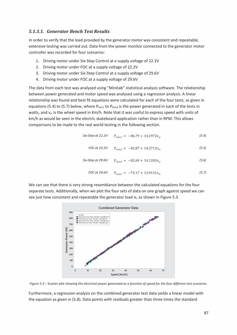
87
5.1.3.1. Generator Bench Test Results
In order to verify that the load provided by the generator motor was consistent and repeatable, extensive testing was carried out. Data from the power monitor connected to the generator motor controller was recorded for four scenarios:
1. Driving motor under Six-Step Control at a supply voltage of 22.2V 2. Driving motor under FOC at a supply voltage of 22.2V 3. Driving motor under Six-Step Control at a supply voltage of 29.6V 4. Driving motor under FOC at a supply voltage of 29.6V
The data from each test was analysed using “Minitab” statistical analysis software. The relationship between power generated and motor speed was analysed using a regression analysis. A linear relationship was found and best fit equations were calculated for each of the four tests, as given in equations (5.4) to (5.7) below, where PGen1 to PGen4 is the power generated in each of the tests in watts, and vw is the wheel speed in Km/h. Note that it was useful to express speed with units of km/h as would be seen in the electric skateboard application rather than in RPM. This allows comparisons to be made to the real world testing in the following section.
Six-Step at 22.2V: (5.4)
FOC at 22.2V: (5.5)
Six-Step at 29.6V: (5.6)
FOC at 29.6V: (5.7)
We can see that there is very strong resemblance between the calculated equations for the four separate tests. Additionally, when we plot the four sets of data on one graph against speed we can see just how consistent and repeatable the generator load is, as shown in Figure 5.3.
Figure 5.3 – Scatter plot showing the electrical power generated as a function of speed for the four different test scenarios.
Furthermore, a regression analysis on the combined generator test data yields a linear model with the equation as given in (5.8). Data points with residuals greater than three times the standard
706050403020100
900
800
700
600
500
400
300
200
100
0
Speed [km/h]
Gene
rato
r Pow
er [W
]
6Step Generator Power 22V [W] * Speed[km/h]_1FOC Generator Power 22V [W] * Speed[km/h]6Step Generator Power 30V [W] * Speed[km/h]_3FOC Generator Power 30V [W] * Speed[km/h]_2
Variable
Combined Generator Data

88
residual value were considered to be strong outliers and were removed from the data set to prevent those data points from skewing the results.
(5.8)
This model results in a residual-squared value of 99.89% indicating a very strong fit for the data. The Minitab residual plots show that there are patterns in the residual data, as given in Figure 5.4. One cause of this may be due to the error in the power and speed measurements which appears to be greater at higher load and speed. Also due to the order of the data points; the data for the second scenario was added to the end of the data from the first scenario, and similarly for the third and fourth scenarios. However, the model was considered to be representative of the relationship between power generated for the given motor speed.
Figure 5.4- Minitab residual plots output for the regression analysis of the combined generator power as a function of speed
tests.
With the electrical power output from the generator motor proven to be consistent and repeatable, it was deemed appropriate to use the model for the combined generator test scenarios as the power generated predictor when testing the driving motor under Six-Step control and FOC.
Refer to Appendix E for the full Minitab data analysis.
5.1.3.2. Six-Step Control Bench Test Results
An identical test to the ones performed while measuring the generator power output was carried out with the driving motor being controlled by Six-Step Control, and the power monitor moved to measure the driving motor controller input power.

89
Analysis of the data was carried out using Minitab. Similarly to the generator tests, a regression analysis with a linear model was used to obtain an equation to predict the power input to the motor controller for a given speed. Again data points with residuals greater than three times the standard residual value were considered to be strong outliers and were removed from the data set. The linear line of best fit model is given in Equation (5.9).
(5.9)
This model results in a residual-squared value of 99.75% indicating a very strong fit for the data. Additionally the Minitab residual plots indicate that the model is again a very strong fit to the data with patterns in the residual plots explained by the apparent increase in error at high speed and load, and the data being ordered from highest speed to lowest speed. This model was considered to be representative of the relationship between the power input and motor speed for the driving motor controller under Six-Step Control.
5.1.3.3. FOC Bench Test Results
Again, an identical test to the ones performed while measuring the generator power output was carried out with the driving motor being controlled by FOC with the power monitor measuring the driving motor controller input power.
The data was analysed using Minitab. Similarly to the previous tests, a regression analysis with a linear model was used to obtain an equation to predict the power input to the motor controller for a given speed. Again, data points with residuals greater than three times the standard residual value were considered to be strong outliers and were removed from the data set. The linear line of best fit model is given in Equation (5.9).
(5.7)
This model results in a residual-squared value of 99.94% indicating a very strong fit for the data. The Minitab residual plots again shows a pattern of greater residuals with greater speed due to the suspected error in power and speed measurement increasing with load and speed. This is reinforced in the plot of residual vs. observation order. The model was considered to be representative of the relationship between the power input and motor speed for the driving motor controller under FOC.
5.1.4. Bench Testing Conclusions
In order to draw any real conclusions on the relative performance between the motor controller under Six-Step control and FOC, it is useful to plot the models as formulated in the previous sections. Figure 5.5 shows the three line of best fit models on one plot.

90
Figure 5.5 - Graphical representation of the linear line of best fit models for power input under Six-Step Control and FOC,
and power generated as a function of motor speed.
We can see that there is a slight difference in the amount of power input required to drive the load between Six-Step Control and FOC. This is more predominant at low speeds.
Next we compare the overall system efficiency of the motor-generator setup. This includes all the power losses in the driving motor and motor controller as well as the generating motor and motor controller. Total system efficiency for the driven motor under Six-Step Control is calculated using equations (5.10) and (5.11) below.
(5.10)
(5.11)
Total system efficiency for the driven motor under FOC is calculated using equations (5.12) and (5.13) below.
(5.12)
(5.13)
Plotting these two equations yields Figure 5.6.
70605040302010
1200
1000
800
600
400
200
0
Speed [km/h]
Powe
r [W
]
Power in [W] 6StepPower in [W] FOCPower out [W]
Variable
Six-Step, FOC, and Generated Power fitted lines

91
Figure 5.6 - Graphical representation of the bench test setup total system efficiency for the driven motor under Six-Step
Control and FOC.
From this we can see that the motor driven under FOC has a greater efficiency than that of Six-Step Control at low speeds. However at higher speeds, the motor driven under Six-Step Control appears to have an advantage in efficiency for these implementations of Six-Step Control and FOC.
The maximum efficiency achieved during this testing of 0.73. If we make the assumption that the generator motor and motor controller have approximately the same efficiency as the driving motor and motor controller (all components of the drive side and generator side are identical), then we can say that the maximum efficiency of the drive motor and motor controller seen in this testing is around 0.865.
Also worth noting is that the overall system efficiency for both Six-Step Control and FOC has a positive slope at the point where the tests ended. This indicates that the maximum efficiency point was not reached. To find this maximum efficiency point, the tests need to be run to a higher speed which would be possible using a higher voltage. However given the maximum rating of the motor controllers is 40V, it was decided not to pursue higher voltage testing for the risk of blowing the motor controllers due to voltage spikes caused by the power supply when its load is decreased suddenly.
The final figure in this analysis shows the difference in efficiency between the two control techniques, Δηtotal given by equations (5.14) and (5.15) below.
(5.14)
(5.15)
Plotting this equation yields the difference in total system efficiency for Six-Step Control and FOC against speed as shown in Figure 5.7.
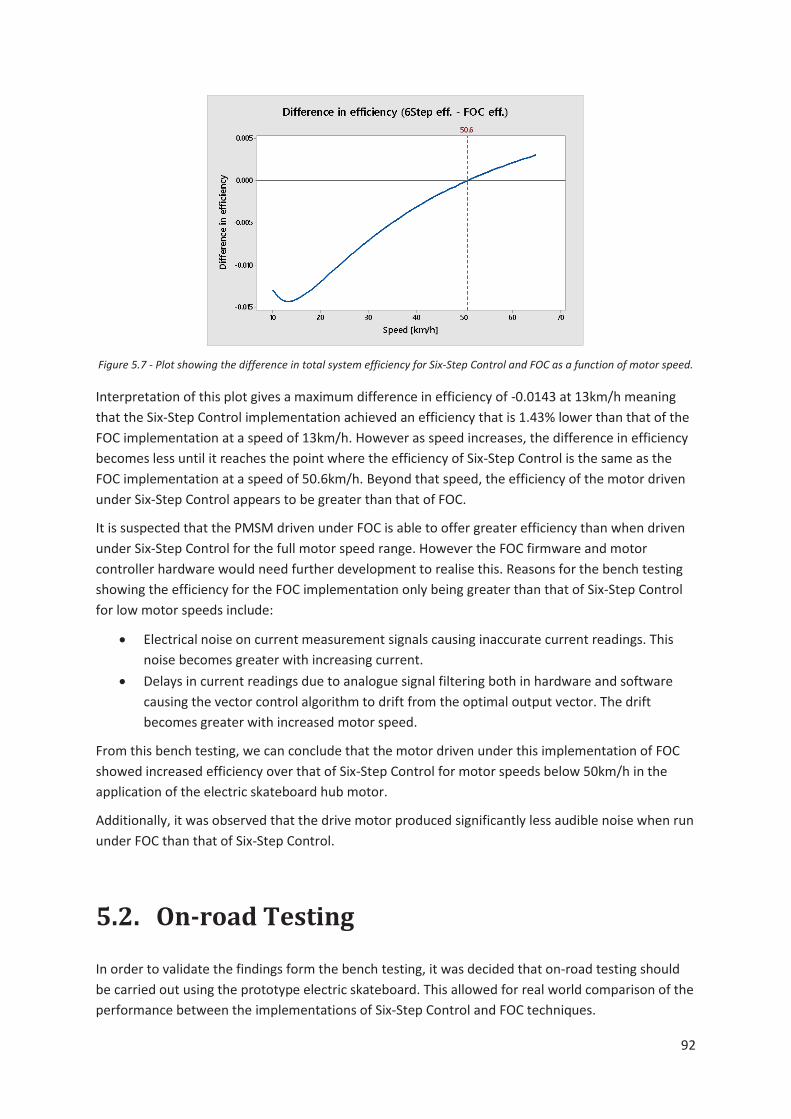
92
Figure 5.7 - Plot showing the difference in total system efficiency for Six-Step Control and FOC as a function of motor speed.
Interpretation of this plot gives a maximum difference in efficiency of -0.0143 at 13km/h meaning that the Six-Step Control implementation achieved an efficiency that is 1.43% lower than that of the FOC implementation at a speed of 13km/h. However as speed increases, the difference in efficiency becomes less until it reaches the point where the efficiency of Six-Step Control is the same as the FOC implementation at a speed of 50.6km/h. Beyond that speed, the efficiency of the motor driven under Six-Step Control appears to be greater than that of FOC.
It is suspected that the PMSM driven under FOC is able to offer greater efficiency than when driven under Six-Step Control for the full motor speed range. However the FOC firmware and motor controller hardware would need further development to realise this. Reasons for the bench testing showing the efficiency for the FOC implementation only being greater than that of Six-Step Control for low motor speeds include:
Electrical noise on current measurement signals causing inaccurate current readings. This noise becomes greater with increasing current.
Delays in current readings due to analogue signal filtering both in hardware and software causing the vector control algorithm to drift from the optimal output vector. The drift becomes greater with increased motor speed.
From this bench testing, we can conclude that the motor driven under this implementation of FOC showed increased efficiency over that of Six-Step Control for motor speeds below 50km/h in the application of the electric skateboard hub motor.
Additionally, it was observed that the drive motor produced significantly less audible noise when run under FOC than that of Six-Step Control.
5.2. On-road Testing
In order to validate the findings form the bench testing, it was decided that on-road testing should be carried out using the prototype electric skateboard. This allowed for real world comparison of the performance between the implementations of Six-Step Control and FOC techniques.
93
5.2.1. Test Rig
The test rig used for this on road testing is simply the hub motor driven electric skateboard prototype as described in detail in section 3. To recap, the prototype electric skateboard contains a 6 cell, 20Ah Lithium Polymer battery pack with nominal voltage of 22.2V. The battery provides energy to the two custom built three phase motor controllers. The motor controllers are each connected to a separate motor which propels the skateboard. The amount of power that the motor controllers feed to the motors is controlled by a handheld wireless RC transmitter with its receiver connected to the two motor controllers throttle input.
The same power meter that was used for the bench testing was mounted on the electric skateboard to measure the electrical power input to one of the two motor controllers.
Similarly to the bench testing, the data logging function of the power meter was used to record data at a frequency of 4Hz to be used for this analysis. As the two motors and motor controllers are identical, we can safely assume that the data obtained for the monitored motor controller is representative of the second, unmonitored motor controller.
The connection between the power meter and the motor controller allows it to measure input voltage, current, power, and energy used. The pulse input to the power meter was connected to the output from one of the hub motor’s internal mounted hall sensors to allow for speed measurements. Both hub motors also have digital temperature sensors installed in the stator windings. These were connected to the power meter external temperature input to allow for measurement of the two motors winding temperatures.
5.2.2. Test Setup
To enable fair comparisons to be made between two the two motor control techniques, a test setup must be devised that can be replicated to a high degree of accuracy for two separate runs. The speed profiles of the two runs should be as similar as possible, ideally with the same acceleration rate, same final speed, same deceleration rate, and same distance travelled. While its noted that it would be near impossible to achieve the exact same speed profile, all attempts should be taken to make the two test runs as similar as possible so that the results from this testing are non-biased.
An ideal test route would consist of a long straight stretch of road or sealed path to allow for the electric skateboard rider to accelerate up to the final speed at a minimal acceleration, and decelerate to a complete stop at a minimal deceleration rate. Any obstacles such as other users of the test route or sharp corners that require slowing down for effect the repeatability of the test.
A suitable sealed path was selected for the on road testing; a cycleway in Lower Hutt City which runs alongside the Hutt River. The testing was conducted along a stretch of this cycle way starting from “Bridge Street” to “Block Road”. This stretch has no tight corners or hills. This particular stretch of the path is least used by members of the public as there is a second path nearer the river and a third path on the other side of the river therefore less chance that the tests would be interrupted.
A test was designed that would allow for comparisons of range and efficiency between the two motor control techniques. Beginning and end points were defined at the ends of the test route so that the total distance travelled for each run is identical. Additional points were defined for end of

94
acceleration and start of deceleration in an attempt to match the acceleration and deceleration rates. A return trip was used for the tests so that any effects from wind and change in elevation between start and end points can be neglected. The start and stop points for one direction of the test track are 1027m apart in distance which would see a return trip totalling 2.054km. It was decided that the on-road testing may be more accurate over a longer distance therefore the return trip was completed multiple times for a single test run. A map showing the test route is given in Figure 5.8 illustrated by the blue line.
Figure 5.8 - Map showing the route used for the on-road testing.
A second on-road test was designed to make comparisons of top speed and power between the two control technique implementations. This test was carried out within the same section of the Hutt River cycleway using only the first 450m starting from the Bridge Street end. This test involves accelerating as quickly as possible up to the maximum speed, followed by decelerating as quickly as possible down to a complete stop using the regenerative braking function. This test was also conducted as a return trip so that the effects of wind and change in elevation can be considered.
The power and speed tests were repeated three times sequentially without charging the battery in between test runs as it was deemed that the battery capacity usage for a single test is small and therefore will not significantly reduce the battery voltage for the following tests.
5.2.3. Test Results
The data log files from the on-road tests were transferred from the power meter to a computer for analysis using Microsoft Excel.
5.2.3.1. Range and Efficiency Test
As mentioned in the previous section, the speed profiles for the Six-Step Control and FOC tests would ideally be identical. In practise this is not easily achieved. In order to make any meaningful

95
comparisons between the two test runs, we must first verify that the speed profiles are similar. The speed profiles are best examined by simply plotting speed against time for the two test runs. The speed profile for one complete test run of the Six-Step Control range and efficiency test run is displayed in Figure 5.9.
Figure 5.9 - Speed profile for Six-Step Control range and efficiency on-road test number 3 (raw data).
The speed profile for one test run of the FOC range and efficiency test run is displayed in Figure 5.10.
Figure 5.10 - Speed profile for FOC range and efficiency on-road test number 3 (raw data).
It is difficult to inspect how similar the two runs are in their raw format due to differences in start times and wait times in between passes of the test route. The time periods where the electric skateboard was stationary were removed from the data. This includes the time period before the test started, the time periods at a standstill in between passes of the test route, and the time period after the test had been completed. With the inactive time periods removed from the data sets, the two speed profiles can be plotted on the same chart and examined for similarity as shown in Figure 5.11.

96
Figure 5.11 – Range and efficiency on-road test 3 speed profiles for both Six-Step Control and FOC with inactive periods
removed.
After running the tests numerous times to get the above results, the speed profiles from the two test runs were deemed to be similar enough to make fair comparisons between the range and efficiency achieved by Six-Step Control and FOC.
The range and efficiency test was repeated three times. It was found that there was large variance in energy consumption from one test to another. This can only be attributed to external influences such as wind strength. A summary of the three runs is shown in Table 5.1.
Control Technique
Test Number
Average Speed [km/h]
Start Battery Voltage [V]
Energy Consumption [Wh/km]
Calculated Range [km]
Six-Step Control
Test 1 32.65 23.82 13.65 32.19
Test 2 33.15 24.57 13.73 32.33
Test 3 33.18 24.52 11.87 37.41
Average 32.99 24.30 13.08 33.98
Field Oriented Control
Test 1 32.68 24.53 14.33 30.99
Test 2 31.85 24.5 11.96 37.12
Test 3 32.71 24.48 10.35 42.89
Average 32.41 24.50 12.21 37.00
Table 5.1 - Summary of on-road testing range and efficiency tests for Six-Step Control and FOC techniques.
5.2.3.2. Power and Speed Test
A typical speed test would see the speed being measured in both directions along a straight stretch of road. The lower of the two speed measurements would be taken as the maximum speed of the vehicle. The same approach was used for the speed test of the electric skateboard when controlled

97
under both Six-Step Control and FOC. The instantaneous speed measurements for a single return trip are plotted against time in Figure 5.12 for both of the motor control techniques.
Figure 5.12 - Instantaneous speed measurements for both directions of a single run for Six-Step Control (left) and FOC (right) techniques.
Evidently, the return direction was slower for both of the tests due to a head wind while travelling in that direction. Therefore the data for the return direction was used for further analysis of the speed and power tests.
Three test runs were completed for each of the motor control techniques so that the results can be proven to be consistent and a higher level of confidence can be placed. The three runs for each test are plotted in Figure 5.13 below.
Figure 5.13 - Instantaneous speed measurements for three runs return pass only for Six-Step Control (left) and FOC (right) techniques.
A notable observation is that Run 2 of the FOC speed test was slower to accelerate than the other two runs. However the maximum speed achieved in Run 2 is similar to that of the other tests for FOC.
We can also take readings of acceleration from the data. The time it takes to accelerate from 0 – 40km/h was nominated as the measure of acceleration. Similarly, the time it takes to decelerate from 40 – 0 km/h was nominated as the measure of deceleration. These readings are also expressed as SI units, m.s-2 in Table 5.2 below which summarises the data from the speed tests.
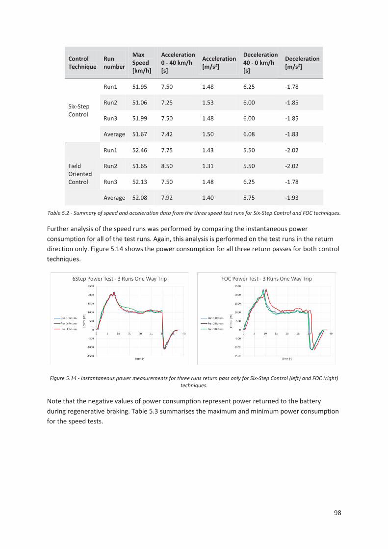
98
Control Technique
Run number
Max Speed [km/h]
Acceleration 0 - 40 km/h [s]
Acceleration [m/s2]
Deceleration 40 - 0 km/h [s]
Deceleration [m/s2]
Six-Step Control
Run1 51.95 7.50 1.48 6.25 -1.78
Run2 51.06 7.25 1.53 6.00 -1.85
Run3 51.99 7.50 1.48 6.00 -1.85
Average 51.67 7.42 1.50 6.08 -1.83
Field Oriented Control
Run1 52.46 7.75 1.43 5.50 -2.02
Run2 51.65 8.50 1.31 5.50 -2.02
Run3 52.13 7.50 1.48 6.25 -1.78
Average 52.08 7.92 1.40 5.75 -1.93
Table 5.2 - Summary of speed and acceleration data from the three speed test runs for Six-Step Control and FOC techniques.
Further analysis of the speed runs was performed by comparing the instantaneous power consumption for all of the test runs. Again, this analysis is performed on the test runs in the return direction only. Figure 5.14 shows the power consumption for all three return passes for both control techniques.
Figure 5.14 - Instantaneous power measurements for three runs return pass only for Six-Step Control (left) and FOC (right) techniques.
Note that the negative values of power consumption represent power returned to the battery during regenerative braking. Table 5.3 summarises the maximum and minimum power consumption for the speed tests.
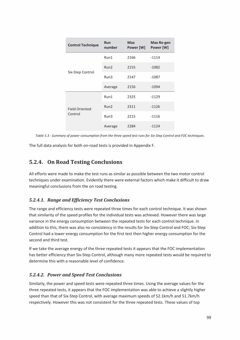
99
Control Technique Run number
Max Power [W]
Max Re-gen Power [W]
Six-Step Control
Run1 2166 -1114
Run2 2155 -1082
Run3 2147 -1087
Average 2156 -1094
Field Oriented Control
Run1 2325 -1129
Run2 2311 -1126
Run3 2215 -1116
Average 2284 -1124
Table 5.3 - Summary of power consumption from the three speed test runs for Six-Step Control and FOC techniques.
The full data analysis for both on-road tests is provided in Appendix F.
5.2.4. On Road Testing Conclusions
All efforts were made to make the test runs as similar as possible between the two motor control techniques under examination. Evidently there were external factors which make it difficult to draw meaningful conclusions from the on road testing.
5.2.4.1. Range and Efficiency Test Conclusions
The range and efficiency tests were repeated three times for each control technique. It was shown that similarity of the speed profiles for the individual tests was achieved. However there was large variance in the energy consumption between the repeated tests for each control technique. In addition to this, there was also no consistency in the results for Six-Step Control and FOC; Six-Step Control had a lower energy consumption for the first test then higher energy consumption for the second and third test.
If we take the average energy of the three repeated tests it appears that the FOC implementation has better efficiency than Six-Step Control, although many more repeated tests would be required to determine this with a reasonable level of confidence.
5.2.4.2. Power and Speed Test Conclusions
Similarly, the power and speed tests were repeated three times. Using the average values for the three repeated tests, it appears that the FOC implementation was able to achieve a slightly higher speed than that of Six-Step Control, with average maximum speeds of 52.1km/h and 51.7km/h respectively. However this was not consistent for the three repeated tests. These values of top

100
speed for both motor control techniques are very similar with only 0.43km/h difference between the averaged top speeds. Therefore it is concluded that there is no significant difference in the top speed between this implementation of Six-Step Control and FOC.
The Six-Step Control implementation was able to accelerate faster than the FOC implementation with an acceleration of 1.50ms-2 compared to 1.40ms-2. Although it should be noted that acceleration is a result of motor torque and is directly related to the amount of motor current, therefore acceleration depends on accuracy of the motor controller current limiting function. This will be different for each of the control techniques and therefore the power consumption should also be considered. The average maximum power consumption during acceleration was lower with Six-Step Control than it was with FOC, using 2156W compared to 2284W. This indicates that the Six-Step Control implementation was able to accelerate faster and used less power to do so.
From this we may conclude that the Six-Step Control implementation had better performance than the FOC implementation under high power demands, similar to what was seen in the bench testing. This is most likely due to the causes outlined in section 5.1.4 where the FOC implementation is not running at optimal conditions due to inaccuracies in current readings under high motor speed and load which may lead to the output voltage vector deviating from the optimal vector.

101
6. Improvements
The prototype electric skateboard was more than adequate in providing a platform on which testing of the motor control techniques could be completed. However there are some improvements which are recommended if any further development were to be pursued. This section will discuss some of the author’s ideas for improvements to the electric skateboard prototype.
6.1. Hub Motor Improvements
The hub motor that was used in the electric skateboard prototype was built by modifying a low cost PMSM that was originally designed for use in a large scale RC aeroplane. Clearly there are certain aspects of such motor that should be changed in order to optimise it for the electric skateboard hub motor.
6.1.1. Larger Bearings
The specific motor was chosen as one which has a bearing to support the outer rotor at both ends to cope with the radial loads that it is subject to in the hub motor application. However, the bearing at the outside end of the hub motor is small with dimensions 8mm bore, 12mm OD, and 3.5mm width. This bearing has been identified as a weak point of the hub motor assembly. Unfortunately the bearing housing does not have sufficient material to machine out for a larger bearing.
To eliminate this weak point, a custom rotor end support should be fabricated which allows for a larger diameter bearing housing. A standard size skateboard bearing should be used as the replacement which has dimensions 8mm bore, 22mm OD, and 7mm width.
6.1.2. Skateboard Wheel Mechanical Fixing
Currently the skateboard wheel is attached to the motor rotor by means of an adhesive and an interference fit. When the wheel becomes worn, it will be difficult to replace. An improvement to this would be to insert an aluminium cylinder as an intermediate interface. The skateboard wheel would attach to this cylinder in the same manner as it is currently attached to the rotor. The cylinder would bolt on to the rotor. The intermediate cylinder would be a disposable part which is discarded with the worn wheels.
6.1.3. Custom Wound Stator
Re-winding the stator for different torque and speed characteristics could offer improvements in efficiency. A motor that takes more voltage and less current for a given speed and torque output is likely to offer improved efficiency due to lower resistive loses which are proportional to the square
102
of current. The torque and speed characteristics can also be optimised for the electric skateboard hub motor application in order to find a good balance between acceleration / hill climbing ability and the maximum speed at which it can travel.
Re-winding the motor also offers scope for increasing the cross sectional area of the phase conductors. Larger cross sectional area will give lower phase resistance and therefore less resistive power loss and heating of the windings. The original motors used for the hub motor conversion are mass produced. For ease of production, the phase windings are made up of many fine wires in parallel. The enamel insulation on the individual wires adds to the diameter of each wire. If a single large wire is used, the total cross sectional area of the insulation is reduced leaving more area for the conductor material.
6.2. Motor Controller
As with any electronic equipment under development, there are many improvements that could be made in both hardware and software.
6.2.1. Miniaturisation
A notable improvement would be to reduce the overall size of the motor controllers by using smaller size surface mount components and having the PCBs professionally assembled.
The PCBs could also be designed on a four layer PCB which would also allow for a smaller size footprint. This also has the advantage that it allows for improved digital and analogue small signal quality by using internal PCB layers for the small signal carrying traces and ground planes on the outside layers.
6.2.2. Current Sensing Improvements
In addition to using a four layer PCB, current sensing could be improved by adapting a component placement that aims to minimise the length of the current sensing analogue signals and keeping these signals separated from any digital signals and power carrying traces. This would help to reduce electrical noise in the current measurement, allowing for reduced hardware and software signal filtering.
6.2.3. Fast Over-current Protection
It was discovered that the inputs to the comparator peripherals of the microcontroller could not be multiplexed internally to the OPAMP outputs. An improvement would be to route the comparator input pins to the OPAMP output pins on the Control PCB. This would allow the comparators to be used as a very fast acting over current protection as their outputs can be used to directly interrupt the motor control timer to turn off all outputs to the semiconductor switches.

103
6.3. General Improvements
This section offers some ideas for general improvements to the electric skateboard prototype in order to increase the ease of use and long term reliability.
6.3.1. Battery Isolator
Currently the battery pack is connected to the motor controllers using individual power plugs on each of the DC input wires. These plugs are located inside the enclosure and need to be manually disconnected after each use of the electric skateboard. A more convenient means of battery isolation would increase the ease of use. The proposed improvement is to add a semiconductor power switch connected in between the battery pack and motor controllers. This semiconductor switch would be controlled by a low current mechanical switch such as a latching pushbutton switch or a key operated switch for added security.
The motor controllers have a large amount of capacitance on the DC power rails. Then the battery is first connected by a mechanical switch, it creates a significant arc due to the inrush of current to charge the capacitors. Arcing damages the contacts of the mechanical switch or plugs and therefore any mechanical switch would be subject to a short lifecycle before failure unless a capacitor pre-charge circuit is installed. The pre-charge circuit initially charges the capacitors through a current limiting resistor before the main contact closes. The semiconductor switch does not create any arcing which removes the need for a capacitor pre-charge circuit.
6.3.2. Weight Reduction
While the electric skateboard prototype could already be considered to be sufficiently lightweight as is, any weight reductions can increase its ease of transport. Currently the prototype weighs 8.6kg which is light enough that it can be carried reasonably easily in one hand. However after extended periods of time, it does become ‘heavy’. One of the leading uses of the electric skateboard is what some authors refer to as “the last mile” of a commute. In this application, the user may be required to carry the electric skateboard for an extended period of time.
A simple weight reduction would be to remove some of the battery capacity. The current battery configuration is ‘6S4P’ Lithium Polymer cells, which gives 20Ah at 22.2V nominal voltage. This configuration has proven to give ample range – over 35km at a final speed of 40km/h with numerous starts/stops. This is more than necessary for a typical skateboard trip. Reducing the battery to ‘6S3P’ configuration to give 15Ah at 22.2V nominal voltage would reduce the weight by 824g and would have an expected range of over 26km under the same conditions.
There is also scope to reduce the weight of the skateboard deck. A skateboard deck could be custom made for the electric skateboard application. This could be constructed of carbon fibre with a built in enclosure for the batteries and electronics. The added thickness of the deck from an electronics enclosure inherently provides a stronger design than a thin planar deck. This would of course, result in a rigid skateboard deck which would alter the handling characteristics which may be an undesirable effect.

104
6.3.3. Water Resistance
The electric skateboard electronics enclosure would benefit from having increased water resistance for instances where it is used on wet grounds. This would reduce the risk of damaging the electronics due to water damage and reduce the risk of receiving an electric shock from the battery. If the electronics enclosure were to be rebuilt, this issue would be given a higher level of consideration.

105
7. Concluding Remarks
To conclude this report, the following sections offer the Author’s final comments on the hub motors and motor controllers built for the electric skateboard prototype as well as some conclusions to be taken from the tests conducted in an attempt to compare the performance of the Six-Step Control and FOC motor control techniques.
7.1. Complete Prototype
The complete electric skateboard prototype has exceed expectations in that it has exceeded the specifications set forth in the design objectives as given in section 1.3. The prototype was able to maintain a speed of over 51km/h and could achieve a range of over 32km at a final speed of 40km/h with numerous starts and stops on a single battery charge. The electric skateboard weighs 8.6kg and is easy to carry for use in “the last mile” of public transportation.
7.2. Hub Motor
The direct drive hub motor system built for the electric skateboard prototype has proven to be a highly feasible option and offers numerous advantages over typical externally mounted motors. At the time of starting this project, there were no such drive systems available for electric skateboard applications. However there are now companies developing an electric skateboard using a hub motor design, the “Inboard M1” which is being released in June 2016, and the “Mellow Board” which is being released in September 2016.
The electric skateboard prototype has shown that the hub motor drive system is able to provide exceptional performance for an electric skateboard. The dual hub motor setup used in this project was able to reach speeds of over 50km/h and sustain power levels in excess of 2kW of input power. In fact, the performance is currently only limited by the battery voltage. Simply installing a higher voltage battery would see increases in top speed and power.
The current top speed of over 50km/h could be considered excessive. There is also scope for reducing the performance of the hub motor drive system using a single motor or two smaller motors. This would allow for some cost savings and weight reduction. However as a prototype designed as proof of concept, the drive system has exceeded expectations.

106
7.3. Motor Controller
The motor controllers built for this project has provided a suitable platform on which the testing of motor control techniques could be performed. The motor controllers themselves performed adequately. However there is much scope for further development and refinement of the motor controller hardware for improved performance. Some general suggestions for improvements to the motor controller hardware were offered in the previous section. It is believed that further development of the motor controller hardware would see the FOC motor control implementation being able to provide better performance than that of Six-Step Control over the full range of speed and load.
7.4. Motor Control Techniques
Two motor control techniques were selected for comparisons to be made between the performance of a PMSM driven under the different control techniques. The PMSM used in this project is a relatively small motor with a diameter of 59mm and power rating of 2250W. This motor is designed for use in large scale RC aeroplanes but has also proven to be highly suitable in LEV applications. Such a motor would typically be driven by low cost hobby grade motor controllers using the basic motor control technique of Six-Step Control. For this reason, Six-Step Control was selected as one of the motor control techniques for examination which has provided a reference to which a second motor control technique could be compared. FOC was identified as an advanced motor control technique that could offer increased performance of the PMSM.
The theory behind the two motor control techniques shows that FOC should be able to drive a PMSM more efficiently than when driven under Six-Step Control. The output voltage vector of the inverter under Six-Step Control is limited to six discrete directions whereas under FOC, the inverter output voltage vector is continuously variable in direction and magnitude using SVM. SVM allows for the motor to be controlled such that the inverter output voltage vector is placed on the quadrature axis therefore maximising the torque of the motor for a given motor current.
Bench testing was conducted using a motor to drive a generator as the load. It was shown that the generator was able to provide a load which is directly proportional to motor speed and is highly consistent and repeatable. This allowed for comparisons of the performance of the motor when driven under Six-Step Control compared to when driven under FOC. It was found that this implementation FOC was able to produce better performance of up to 1.43% more efficient than that of Six-Step Control during this test. However this advantage was only realised at low speed. At speeds greater than 50km/h, Six-Step Control became the more efficient motor control implementation. It is believed that the reason for this is due to imperfections in the motor controller hardware and FOC software causing the inverter output to drift from the optimal output voltage vector at high load and speed.
On-road testing was conducted using the prototype electric skateboard with custom built hub motors as the test rig in order to compare the performance of the two motor control techniques in a real world application. A test designed to compare the efficiency and range of the electric

107
skateboard gave inconclusive comparisons between Six-Step Control and FOC due to large variation and inconsistent results between repeated tests. However we can conclude that the in the worst case scenario, the electric skateboard prototype was able to achieve a range of 31km at a final speed of 40km/h. The Matlab generated simulation discussed in section 3.2.2 predicted a range of 27.7km at 40km/h therefore it can be said that the electric skateboard prototype has exceeded expectations for range.
Furthermore, a second on-road test was designed to compare the top speed and power consumption for the two motor control techniques. It was found that there was no significant difference in the maximum speed from the two motor control technique implementations. It was also found that the Six-Step Control implementation was able to accelerate faster and use less power to do so than the FOC implementation. The acceleration test represents a high load scenario which reinforces what was seen in bench testing where the Six-Step implementation was able to achieve a greater efficiency under high load.
The testing conducted in this project has shown that FOC is able to drive a PMSM more efficiently than Six-Step Control. However imperfections in the motor controller hardware and software has seen this advantage only being realised for low load and low speed scenarios. It is believed that further development of the motor controller hardware and software would see the FOC implementation being more efficient than Six-Step Control over the full load and speed range.

108
8. References
Andrada, P., Blanqué, B., Perat, J. I., & Torrent, M. (2006). Power Losses in Outside-Spin Brushless D.C. Motors. Retrieved July 17, 2015, from International Conference on Renewable Energies and Power Quality: http://www.icrepq.com/PONENCIAS/4.320.ANDRADA.pdf
Atmel. (2013, May 16). AVR32723: Sensor Field Oriented Control for Brushless DC motors with AT32UC3B0256. Retrieved from Atmel: http://www.atmel.com/Images/doc32126.pdf
Benjamin, E. (2011, December). Light Electric Vehicles 2011-2021 Electric Bicycles, Scooters and Allied Vehicles. Retrieved July 25, 2016, from IDTechEx: http://www.idtechex.com/research/reports/light-electric-vehicles-2011-2021-000274.asp?viewopt=showall
Bishop, R. H. (2002). The Mechatronics Handbook. Boca Raton, United States of America: CRC Press.
Buchmann, I. (2015, June 6). Types of Lithium-ion. Retrieved June 25, 2015, from Battery University: http://batteryuniversity.com/learn/article/types_of_lithium_ion
C.N. Huerta-Saucedo, R. A.-S.-R.-C. (2012). Experimental Comparison of Control Techniques for a Permanent Magnet Synchronous Motor. Electrical Engineering, Computing Science and Automatic Control (CCE) (pp. 1-6). Mexico City: IEEE.
Cheever, E. (2005). System Elements. Retrieved July 10, 2015, from Elements of Rotating Mechanical Systems: http://lpsa.swarthmore.edu/Systems/MechRotating/RotMechSysElem.html
Colton, S. W. (2008). Design and Prototyping Methods for Brushless Motors and Motor Control. Cambridge: Massachusetts Institute of Technology.
Dwivedi, S., & Singh, B. (2010). Vector Control Vs Direct Torque Control Comparative Evaluation for PMSM Driv. Power Electronics, Drives and Energy Systems (PEDES) (pp. 1-8). New Delhi: IEEE.
Ecotricity. (2016). Carbon & Electric Vehicle Calculator. Retrieved July 20, 2016, from Ecotricity: https://ecotricity.co.nz/calculator/
Electrical For You. (2011). Questions on Eddy Current or Hysteresis Loss. Retrieved August 14, 2015, from Online Electrical Engineering: http://www.electrical4u.com/questions-and-answers-on-eddy-current-or-hysteresis-loss/
Emadi, A. (2014). Advanced Electric Drive Vehicles. Boca Raton, Florida, United States of America: CRC Press.
Fairchild Semiconductor. (2014, December 18). Design and Application Guide of Bootstrap Circuit for High-Voltage Gate-Drive IC. Retrieved from Fairchild Semiconductor: https://www.fairchildsemi.com/application-notes/AN/AN-6076.pdf
Fiorillo, F. (2004). Measurement and Characterization of Magnetic Materials. San Diego, California, United States of America: Elsevier.
Hiroaki Toda, Z. X. (2004, July). Rotor Eddy-Current Loss in Permanent Magnet Brushless Machines. IEEE Transactions on Magnetics, 40, 2104-2106.
109
International Rectifier. (2012, December). DirectFET Technology Board Mounting Application Note. Retrieved from International Rectifier: http://www.irf.com/technical-info/appnotes/an-1035.pdf
International Rectifier. (2013, April 30). AUIRFS8419-7P HEXFET Power MOSFET. Retrieved from International Rectifier: http://www.irf.com/product-info/datasheets/data/auirfs8409-7p.pdf
Jatskevich, P. A. (2012, June). Filtering ofHall-SensorSignalsforImprovedOperation ofBrushlessDCMotors. IEEE Transactions on Energy Conversion, 27, 547-549.
Jewett, J. W., & Serway, R. A. (2008). Physics for Scientists and Engineers. Belmont, CA, United States of America: Thomson Higher Education.
Jianwen Shao, D. N. (2003). Improved Direct Back EMF Detection for Sensorless Brushless DC (BLDC) Motor Drives. Applied Power Electronics Conference and Exposition (pp. 300-305). Miami Beach: IEEE.
Jiles, D. (1998). Introduction to Magnetism and Magnetic Materials (2nd ed.). Boca Raton, Florida, United States of America: Taylor & Francis Group. Retrieved from https://books.google.co.nz/books?id=axyWXjsdorMC&pg=PA3&dq=&redir_esc=y#v=onepage&q&f=false
Kemet Electronics Corporation. (2013, April 17). Radial Aluminum Electrolytic Capacitors. Retrieved from Kemet: http://www.biakom.com/pdf/ESH_Kemet.pdf
Krause, P., Wasynczuk, O., Sudhoff, S., & Pekarek, S. (2013). Analysis of Electric Machinery and Drive Systems (3rd ed.). Hoboken, New Jersey, United States of America: John Wiley & Sons.
L. Zhong, M. F. (1997, May). Analysis of Direct Torque Control in Permanent Magnet Synchronous Motor Drives. IEEE Transactions on Power Electronics, 12, 528-536.
Lemon, S., & Miller, A. (2013). Electric Vehicles in New Zealand: Technologically Challenged? EEA Conference & Exhibition. Auckland: Electric Power Engineering Centre, University of Canterbury. Retrieved from http://www.epecentre.ac.nz/docs/media/Electric%20Vehciles%20in%20New%20Zealand%20-%20Technologically%20Challenged.pdf
M. S. Merzoug, a. F. (2008). Comparison of Field-Oriented Control and Direct Torque Control for Permanent Magnet Synchronous Motor (PMSM). World Academy of Science, Engineering and Technology, 299-304.
Markowski, P. (2002, November 12). Estimating MOSFET switching losses means higher performance buck converters. Retrieved from EE Times: http://www.eetimes.com/document.asp?doc_id=1225701
Messner, B., & Tilbury , D. (1996). DC Motor Speed: System Modeling. Retrieved July 10, 2015, from Control Tutorials for MATLAB and Simulink: http://ctms.engin.umich.edu/CTMS/index.php?aux=About_Tutorials
Mevey, J. R. (2006). Sensorless Feild Oriented Control of Brushless Permanent Magnet Synchronous Motors. Manhattan: Kansas State University.

110
Microchip Technology Inc. (2003, July 28). Brushless DC (BLDC) Motor Fundamentals. Retrieved from Microchip Technologies: http://ww1.microchip.com/downloads/en/AppNotes/00885a.pdf
Movellan, J. R. (2010, March 27). DC Motors. Retrieved July 10, 2015, from http://mplab.ucsd.edu/tutorials/dc.pdf
Muhlethaler, J., Biela, J., Kolar, J., & Ecklebe, A. (2012, February). Core Losses Under the DC Bias Condition Based. IEEE Transactions on Power Electronics, 27(2), pp. 953-963.
Natural Resources Canada. (2014, March 6). Electric Motors - Energy Efficiency Reference Guide. Retrieved July 3, 2015, from Natural Resources Canada: http://www.nrcan.gc.ca/sites/www.nrcan.gc.ca/files/energy/pdf/energystar/motors-ref-eng.pdf
Nikolay Samoylenko, Q. H. (2007). Improving Dynamic Performance of Low- Precision Brushless DC Motors with Unbalanced Hall Sensors. Power Engineering Society General Meeting (pp. 1-8). Tampa: IEEE.
Owen, J., Strouse, J., & Marcel, M. J. (2011). Sensorless Field Oriented Control Utilizing a Sliding Mode Observer for Control of an Actively-Rectified Permanent Magnet Synchronous Generator. Applied Power Electronics Conference and Exposition (APEC) (pp. 1017-1021). Fort Worth: IEEE.
Salcone, M., & Bond, J. (2009). Selecting Film Bus Link Capacitors For High Performance Inverter Applications. Electric Machines and Drives Conference, 2009. IEMDC '09. IEEE International, 1692 - 1699.
Schmidt, R., Schitter, G., Rankers, A., & Eijk, J. (2014). The Design of High Performance Mechatronics (2nd ed.). Amsterdam, Netherlands: Delft University Press.
ST Microelectronics. (2013, December). STM32F0x/F100xx/F103xx/F2xx/F30x/F4xx PMSM single/dual FOC SDK v3.4. Retrieved from ST Microelectronics: http://www.st.com/st-web-ui/static/active/en/resource/technical/document/user_manual/CD00298474.pdf
ST Microelectronics. (2015, August). RM0316 Reference manual STM32F303xB/C/D/E, STM32F303x6/8, STM32F328x8, STM32F358xC, STM32F398xE advanced ARM-based MCUs. Retrieved from ST Microelectronics: http://www.st.com/web/en/resource/technical/document/reference_manual/DM00043574.pdf
Storey, J. (2011, August 20). Hall Effect Sensor Placement for Permanent Magnet Brushless DC Motors. Retrieved August 6, 2015, from Rocket Science: http://mitrocketscience.blogspot.co.nz/2011/08/hall-effect-sensor-placement-for.html
Texas Instruments. (2011, May). Understanding Thermal Dissipation and Design of a Heatsink. Retrieved from Texas Instruments: http://www.ti.com/lit/an/slva462/slva462.pdf
The Engineering Toolbox. (2000, Januray). Drag Coefficient. Retrieved August 14, 2015, from The Engineering Toolbox: http://www.engineeringtoolbox.com/drag-coefficient-d_627.html
Vishay. (2004, December 2). Power MOSFET Basics: Understanding Gate Charge and Using it to Assess Switching Performance. Retrieved from Vishay: http://www.vishay.com/docs/73217/73217.pdf

111
Vishay Siliconix. (2004, December 2). Power MOSFET Basics: Understanding Gate Charge and Using it to Assess Switching Performance. Retrieved September 11, 2015, from http://www.vishay.com/docs/73217/73217.pdf
Zhang, K., Jianqiu, L. I., Ouyang, M., Jing, G. U., & Yan, M. A. (2011). Electric Braking Performance Analysis of PMSM for Electric Vehicle Applications. Electronic and Mechanical Engineering and Information Technology (EMEIT). 5, pp. 2596-2599. Heilongjiang: IEEE.

112
9. Appendices
Appendix A - Journal Article Published in IEEE International Instrumentation and Measurement Technology Conference (I2MTC 2012)


119
Appendix B - Matlab Script for Simulation of the Electric Skateboard Prototype Performance.

120
%Code written by Alexander Rowe %06/05/13 %Electric Skateboard performance simulation %input parameters: kv = 149; %motor speed constant (RPM/V) D = 0.09; %wheel diameter (m) Rbatt = 0.0055; %internal Battery resistance (ohm)(6S4P battery, 3mOhm each cell) + 10mOhm for wires Vbatt = 22.2; %Battery voltage, nominal (V) Ron = 0.00075; %MOSFET on resistance (ohm) (AUIRFS8409-7) Fpwm = 20000; %PWM frequency (Hz) Rg = 20; %gate resistance (ohm) Cg = 2.5E-8; %gate capacitance (F)(AUIRFS8409-7) Rphase = 0.030; %winding resistance (ohm)(Turnigy sk3 6374 149kv) + wires p = 1.204; %fluid density (kg/m^3) A = 0.36; %Front area of person, side on - 1.8m tall * 0.2m wide (m^2) Cd = 1.1; %drag coefficient of person m = 83.3; %total mass (kg) Cr = 0.030; %coefficient of rolling resistance res = 100; %simulation resolution for speed graid = [0, 2, 4, 6, 8, 10]; %simulation gradients (degrees) spdMax = 60; %simulation max speed (km/h); Eb = 3.7*6*20; %battery energy capacity (Wh)(6S 20Ah Lipo) Vdrive = 12.0; %gate drive voltage (V) Rgate = 20.0; %Total gate resistance (ohm) Vgth = 10; %gate voltage turn on threshold (V)(AUIRFS8409-7) Ke = 1; %eddy current constant N = 18; %number of turns for each stator tooth M = 4; %number of active poles L = 0.045; %stator length (m) R = 0.024; %airgap radius (m) Poles = 7; %magnetic pole pairs Lam = 0.00035; %Lamination thickness (m) Vol = 0.00003366; %Stator core volume (m^3) mass = 0.257; %stator core mass (kg) resistivity = 48e-8; %stator core material resistivity (ohm.m) density = 7650; %stator core material density (kg/m^3) Khys = 1.91; %Hysteresis coefficient u0 = 4e-7*pi; %permeability of free space (T.m/A) u = 5e-3; %permeability of electric steel (T.m/A) Coss = 2620e-12; %FET output parasitic capacitance (F) (AUIRFS8409-7) Qg = 305e-9; %FET total gate charge (c) (AUIRFS8409-7) Vf = 0.8; %body diode forward voltage (V) (AUIRFS8409-7) tdiode = 700e-9 * 2; %time that the diode is conducting per PWM cycle (Deadtime) (s) %Consequential variables km = 1/(kv * ((2*pi)/60)); %motor constant (V/(rad/s)) or (Nm/A) TRC = Rgate * Cg; %RC time constant Ton = -TRC * log(1-(Vgth/Vdrive)); %time to turn on and off the FET (s) ur = u/u0; %relative permeability %---------------------------Calculate Data--------------------------------- powerData = zeros(res,size(graid,2)); efficiencyData = zeros(res,size(graid,2)); distanceData = zeros(res,size(graid,2)); tempData = zeros(res,size(graid,2)); %Spare data array for examining various quantities for i = 1:1:size(graid,2) rad = 0.017453293 * graid(i); %convert deg. to rad j=1; for velocity = 0:((spdMax/3.6)/res):(spdMax/3.6) %velocity in m/s w = velocity * (2*pi)/(pi*D); Fcom = velocity/(pi*D) * Poles * 6; %commutation frequency (Hz) %mechanical power required %Pd = 1/2 * p * velocity^2 * A * Cd * velocity; %power to overcome drag (J/s or W) %Ph = m * 9.81 * sin(rad) * velocity; %power to gain height (J/s or W) %Pf = (m/4) * 9.81 * Cr * 4 * velocity; %power to overcome rolling resistance (W)

121
%Pmech = Pd + Ph + Pf; %mechanical torque required Tdrag = 1/2 * p * velocity^2 * A * Cd * (D/2); Troll = ((m/4) * 9.81 * Cr * 4) * (D/2); Tgrav = (m * 9.81 * sin(rad)) * (D/2); T = Tdrag + Troll + Tgrav; Pmech = T * w; T2 = T/2; %Torque on each motor (Nm) I = T/km; %battery current (A) I2 = I/2; %current through each motor and inverter (A) V = km*w; %required phase Voltage (V) %electrical power losses Pbatt = (I^2)*Rbatt; %battery power loss (W) Pron = I2^2*Ron*2; %power loss due to FET resistance. Two transistors on (W) Psw = Vbatt*I2*Fpwm*Ton; %Switching power loss. switching loss occurs 2 times every
cycle (W) Psw2 = Coss * Vbatt^2 * Fpwm + Qg * Vdrive * Fpwm; %power loss from gate charge, output
capacitance (W) Pdiode = I2 * Vf * tdiode * Fpwm; %power loss through diode conduction (W) Pfet = 2*(Pron + Psw + Psw2 + Pdiode); %Combined power loss for both inverters (W) H = I2 * N * L * 2; %magnet feild H (A.m) B = u * H; %magnet feild strength (T) Pcopper = I2^2*Rphase *2; %copper Power Loss, 2 motors (W) Peddy = (pi^2*B^2*Lam^2*Fcom^2*mass)/(6*1*resistivity*density) *2; %power loss due to
eddy current, 2 motors (W) Phys = Khys*B^1.6*Vol*Fcom *2; %Power loss due to hysteresis, 2 motors (W) Pmotor = Pcopper + Peddy + Phys; %power loss in motors (W) Pelec = Pbatt + Pfet + Pmotor; %Total electrical power loss Pt = Pmech + Pelec;% / em; %total power required (W) et = Pmech/Pt; %total efficiency time = (Eb / Pt) * 60 * 60; %run time (s) distance = velocity * time; %total distance travelled (m) efficiencyData(j,i) = et; powerData(j,i) = Pt/1000; distanceData(j,i) = distance/1000; %distance in km tempData(j,i) = Pfet/2; %If statement to pull specific data %if((j==67) && (i==1)) %40km/h, 0 degree slope %tme = (20 / 40) %20km @ 40km/h takes x hours %energy = Pt * tme %energy required to go 20km @ 40km/h (Wh) %end j=j+1; end end speed = 0:spdMax/res:spdMax; figure(1) plot(speed,powerData(:,:)) title('Power requirement predictions'); xlabel('Velocity [km/h]'); ylabel('Power [kW]'); legend('0 deg','2 deg','4 deg','6 deg','8 deg','10 deg'); figure(2) plot(speed,efficiencyData(:,:)) title('Total System Efficiency'); xlabel('Velocity [km/h]');

122
ylabel('Efficiency'); legend('0 deg','2 deg','4 deg','6 deg','8 deg','10 deg'); figure(3) plot(speed,distanceData(:,:)) title('Range predictions'); xlabel('Velocity [km/h]'); ylabel('Distance [km]'); legend('0 deg','2 deg','4 deg','6 deg','8 deg','10 deg'); figure(4) plot(speed,tempData(:,:)) title('Power loss each inverter'); xlabel('Velocity [km/h]'); ylabel('Power loss [W]'); legend('0 deg','2 deg','4 deg','6 deg','8 deg','10 deg');

123
Appendix C - Altium Designer Printouts of the Motor Controller PCB Design
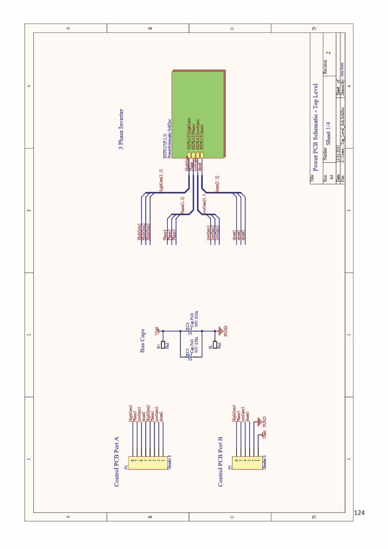
124
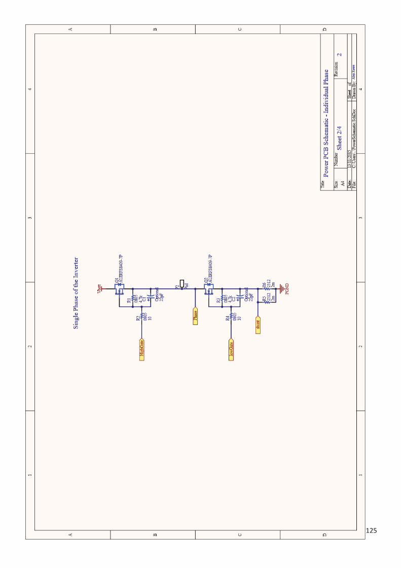
125

126
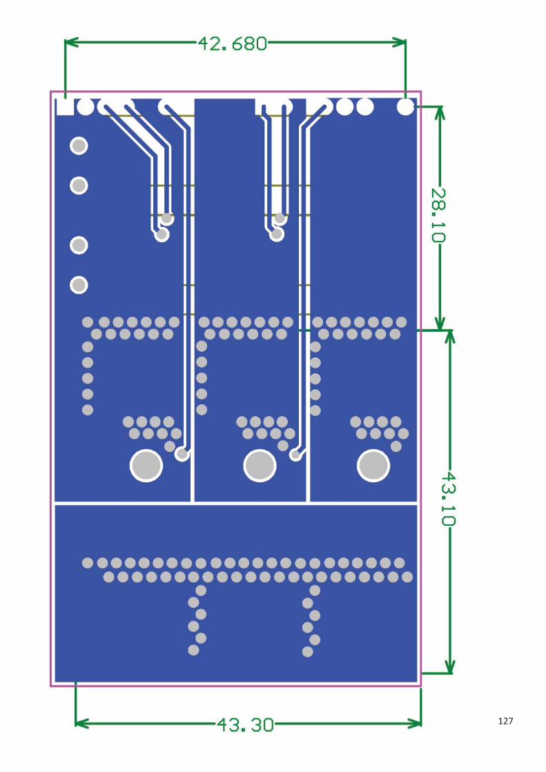
127

128

129
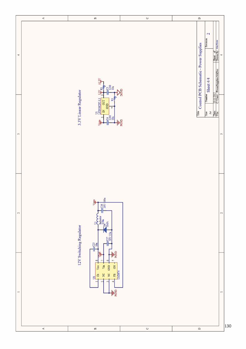
130

131

132

133

134
Appendix D- Motor Controller Firmware Source Code
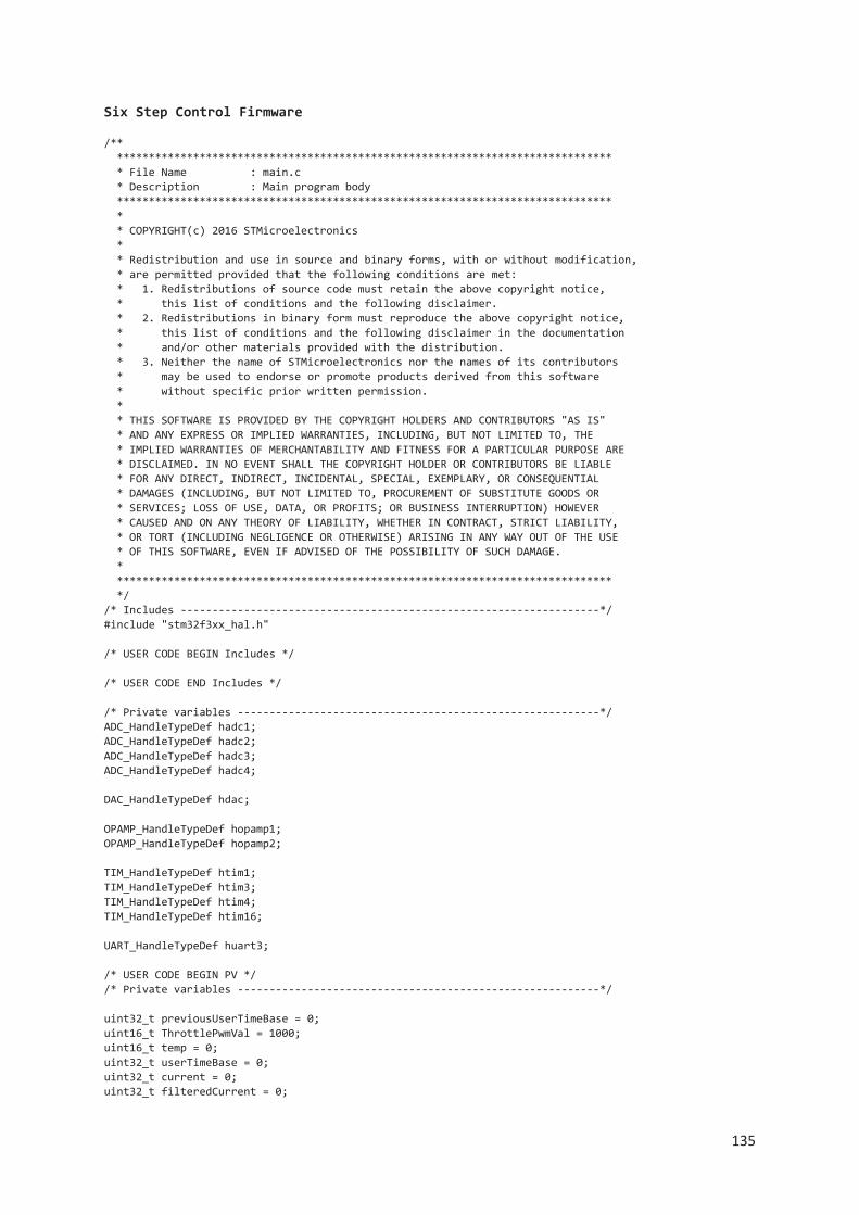
135
Six Step Control Firmware /** ****************************************************************************** * File Name : main.c * Description : Main program body ****************************************************************************** * * COPYRIGHT(c) 2016 STMicroelectronics * * Redistribution and use in source and binary forms, with or without modification, * are permitted provided that the following conditions are met: * 1. Redistributions of source code must retain the above copyright notice, * this list of conditions and the following disclaimer. * 2. Redistributions in binary form must reproduce the above copyright notice, * this list of conditions and the following disclaimer in the documentation * and/or other materials provided with the distribution. * 3. Neither the name of STMicroelectronics nor the names of its contributors * may be used to endorse or promote products derived from this software * without specific prior written permission. * * THIS SOFTWARE IS PROVIDED BY THE COPYRIGHT HOLDERS AND CONTRIBUTORS "AS IS" * AND ANY EXPRESS OR IMPLIED WARRANTIES, INCLUDING, BUT NOT LIMITED TO, THE * IMPLIED WARRANTIES OF MERCHANTABILITY AND FITNESS FOR A PARTICULAR PURPOSE ARE * DISCLAIMED. IN NO EVENT SHALL THE COPYRIGHT HOLDER OR CONTRIBUTORS BE LIABLE * FOR ANY DIRECT, INDIRECT, INCIDENTAL, SPECIAL, EXEMPLARY, OR CONSEQUENTIAL * DAMAGES (INCLUDING, BUT NOT LIMITED TO, PROCUREMENT OF SUBSTITUTE GOODS OR * SERVICES; LOSS OF USE, DATA, OR PROFITS; OR BUSINESS INTERRUPTION) HOWEVER * CAUSED AND ON ANY THEORY OF LIABILITY, WHETHER IN CONTRACT, STRICT LIABILITY, * OR TORT (INCLUDING NEGLIGENCE OR OTHERWISE) ARISING IN ANY WAY OUT OF THE USE * OF THIS SOFTWARE, EVEN IF ADVISED OF THE POSSIBILITY OF SUCH DAMAGE. * ****************************************************************************** */ /* Includes ------------------------------------------------------------------*/ #include "stm32f3xx_hal.h" /* USER CODE BEGIN Includes */ /* USER CODE END Includes */ /* Private variables ---------------------------------------------------------*/ ADC_HandleTypeDef hadc1; ADC_HandleTypeDef hadc2; ADC_HandleTypeDef hadc3; ADC_HandleTypeDef hadc4; DAC_HandleTypeDef hdac; OPAMP_HandleTypeDef hopamp1; OPAMP_HandleTypeDef hopamp2; TIM_HandleTypeDef htim1; TIM_HandleTypeDef htim3; TIM_HandleTypeDef htim4; TIM_HandleTypeDef htim16; UART_HandleTypeDef huart3; /* USER CODE BEGIN PV */ /* Private variables ---------------------------------------------------------*/ uint32_t previousUserTimeBase = 0; uint16_t ThrottlePwmVal = 1000; uint16_t temp = 0; uint32_t userTimeBase = 0; uint32_t current = 0; uint32_t filteredCurrent = 0;

136
uint32_t voltage = 0; uint32_t temperature = 0; #define CURRENT_LIMIT 8000 #define LOW_VOLTAGE_CUTOFF 2040 #define HIGH_TEMP_CUTOFF 6000 /* USER CODE END PV */ /* Private function prototypes -----------------------------------------------*/ void SystemClock_Config(void); static void MX_GPIO_Init(void); static void MX_ADC1_Init(void); static void MX_ADC2_Init(void); static void MX_ADC3_Init(void); static void MX_ADC4_Init(void); static void MX_DAC_Init(void); static void MX_OPAMP1_Init(void); static void MX_OPAMP2_Init(void); static void MX_TIM1_Init(void); static void MX_TIM3_Init(void); static void MX_TIM4_Init(void); static void MX_TIM16_Init(void); static void MX_USART3_UART_Init(void); void HAL_TIM_MspPostInit(TIM_HandleTypeDef *htim); /* USER CODE BEGIN PFP */ /* Private function prototypes -----------------------------------------------*/ /* USER CODE END PFP */ /* USER CODE BEGIN 0 */ uint16_t getThrottlePwmVal(void); void updateThrottle(void); void filterThrottle(uint16_t currentValue); void setDacs(void); uint32_t getFilteredCurrent(uint32_t currentValue); /* USER CODE END 0 */ int main(void) { /* USER CODE BEGIN 1 */ /* USER CODE END 1 */ /* MCU Configuration----------------------------------------------------------*/ /* Reset of all peripherals, Initializes the Flash interface and the Systick. */ HAL_Init(); /* Configure the system clock */ SystemClock_Config(); /* Initialize all configured peripherals */ MX_GPIO_Init(); MX_ADC1_Init(); MX_ADC2_Init(); MX_ADC3_Init(); MX_ADC4_Init(); MX_DAC_Init(); MX_OPAMP1_Init(); MX_OPAMP2_Init(); MX_TIM1_Init(); MX_TIM3_Init(); MX_TIM4_Init();
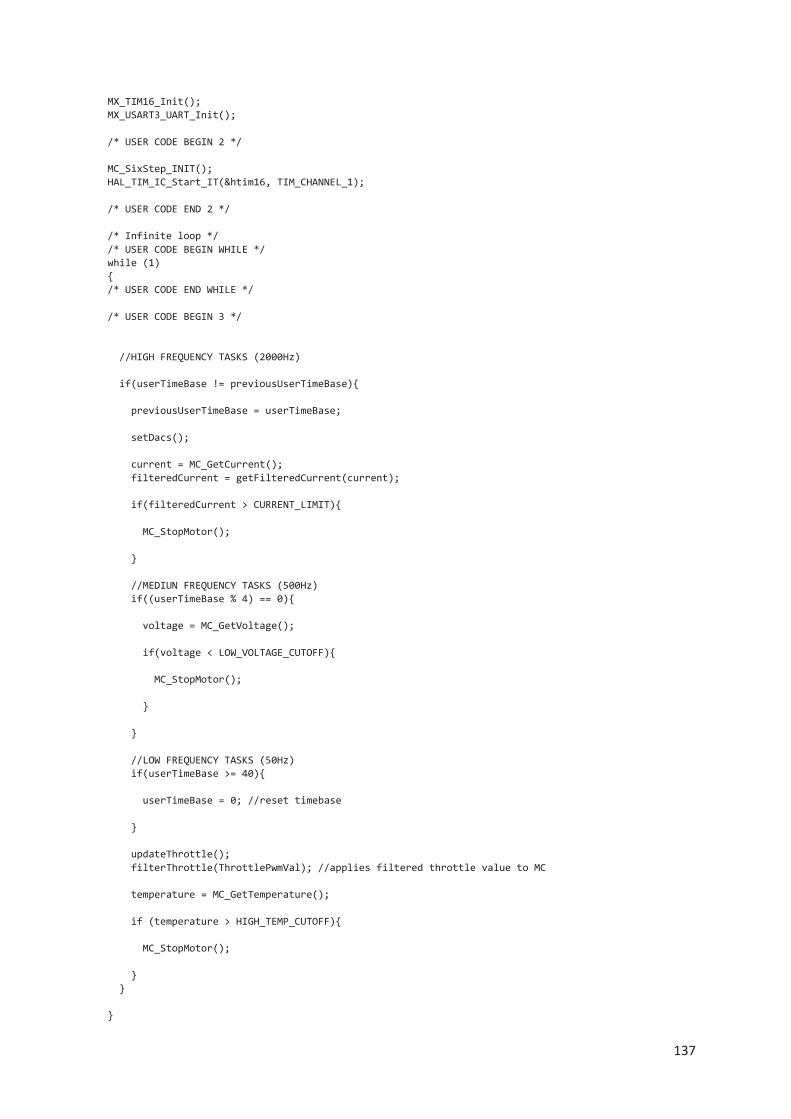
137
MX_TIM16_Init(); MX_USART3_UART_Init(); /* USER CODE BEGIN 2 */ MC_SixStep_INIT(); HAL_TIM_IC_Start_IT(&htim16, TIM_CHANNEL_1); /* USER CODE END 2 */ /* Infinite loop */ /* USER CODE BEGIN WHILE */ while (1) { /* USER CODE END WHILE */ /* USER CODE BEGIN 3 */ //HIGH FREQUENCY TASKS (2000Hz) if(userTimeBase != previousUserTimeBase){ previousUserTimeBase = userTimeBase; setDacs(); current = MC_GetCurrent(); filteredCurrent = getFilteredCurrent(current); if(filteredCurrent > CURRENT_LIMIT){ MC_StopMotor(); } //MEDIUN FREQUENCY TASKS (500Hz) if((userTimeBase % 4) == 0){ voltage = MC_GetVoltage(); if(voltage < LOW_VOLTAGE_CUTOFF){ MC_StopMotor(); } } //LOW FREQUENCY TASKS (50Hz) if(userTimeBase >= 40){ userTimeBase = 0; //reset timebase } updateThrottle(); filterThrottle(ThrottlePwmVal); //applies filtered throttle value to MC temperature = MC_GetTemperature(); if (temperature > HIGH_TEMP_CUTOFF){ MC_StopMotor(); } } }

138
/* USER CODE END 3 */ } /** System Clock Configuration */ void SystemClock_Config(void) { RCC_OscInitTypeDef RCC_OscInitStruct; RCC_ClkInitTypeDef RCC_ClkInitStruct; RCC_PeriphCLKInitTypeDef PeriphClkInit; RCC_OscInitStruct.OscillatorType = RCC_OSCILLATORTYPE_HSE; RCC_OscInitStruct.HSEState = RCC_HSE_ON; RCC_OscInitStruct.HSEPredivValue = RCC_HSE_PREDIV_DIV1; RCC_OscInitStruct.PLL.PLLState = RCC_PLL_ON; RCC_OscInitStruct.PLL.PLLSource = RCC_PLLSOURCE_HSE; RCC_OscInitStruct.PLL.PLLMUL = RCC_PLL_MUL4; HAL_RCC_OscConfig(&RCC_OscInitStruct); RCC_ClkInitStruct.ClockType = RCC_CLOCKTYPE_HCLK|RCC_CLOCKTYPE_SYSCLK |RCC_CLOCKTYPE_PCLK1|RCC_CLOCKTYPE_PCLK2; RCC_ClkInitStruct.SYSCLKSource = RCC_SYSCLKSOURCE_PLLCLK; RCC_ClkInitStruct.AHBCLKDivider = RCC_SYSCLK_DIV1; RCC_ClkInitStruct.APB1CLKDivider = RCC_HCLK_DIV1; RCC_ClkInitStruct.APB2CLKDivider = RCC_HCLK_DIV1; HAL_RCC_ClockConfig(&RCC_ClkInitStruct, FLASH_LATENCY_1); PeriphClkInit.PeriphClockSelection = RCC_PERIPHCLK_USART3|RCC_PERIPHCLK_TIM1 |RCC_PERIPHCLK_ADC12|RCC_PERIPHCLK_ADC34; PeriphClkInit.Usart3ClockSelection = RCC_USART3CLKSOURCE_PCLK1; PeriphClkInit.Adc12ClockSelection = RCC_ADC12PLLCLK_DIV1; PeriphClkInit.Adc34ClockSelection = RCC_ADC34PLLCLK_DIV1; PeriphClkInit.Tim1ClockSelection = RCC_TIM1CLK_PLLCLK; HAL_RCCEx_PeriphCLKConfig(&PeriphClkInit); HAL_RCC_MCOConfig(RCC_MCO, RCC_MCO1SOURCE_SYSCLK, RCC_MCODIV_1); HAL_SYSTICK_Config(HAL_RCC_GetHCLKFreq()/1000); HAL_SYSTICK_CLKSourceConfig(SYSTICK_CLKSOURCE_HCLK); /* SysTick_IRQn interrupt configuration */ HAL_NVIC_SetPriority(SysTick_IRQn, 0, 0); } /* ADC1 init function */ void MX_ADC1_Init(void) { ADC_AnalogWDGConfTypeDef AnalogWDGConfig; ADC_ChannelConfTypeDef sConfig; /**Common config */ hadc1.Instance = ADC1; hadc1.Init.ClockPrescaler = ADC_CLOCK_ASYNC_DIV1; hadc1.Init.Resolution = ADC_RESOLUTION_12B; hadc1.Init.ScanConvMode = ADC_SCAN_DISABLE; hadc1.Init.ContinuousConvMode = DISABLE; hadc1.Init.DiscontinuousConvMode = DISABLE; hadc1.Init.ExternalTrigConvEdge = ADC_EXTERNALTRIGCONVEDGE_NONE; hadc1.Init.DataAlign = ADC_DATAALIGN_RIGHT; hadc1.Init.NbrOfConversion = 1; hadc1.Init.DMAContinuousRequests = DISABLE; hadc1.Init.EOCSelection = ADC_EOC_SINGLE_CONV; hadc1.Init.LowPowerAutoWait = DISABLE; hadc1.Init.Overrun = ADC_OVR_DATA_OVERWRITTEN;

139
HAL_ADC_Init(&hadc1); /**Configure Analog WatchDog 1 */ AnalogWDGConfig.WatchdogNumber = ADC_ANALOGWATCHDOG_1; AnalogWDGConfig.WatchdogMode = ADC_ANALOGWATCHDOG_SINGLE_REG; AnalogWDGConfig.HighThreshold = 4012; AnalogWDGConfig.LowThreshold = 0; AnalogWDGConfig.Channel = ADC_CHANNEL_3; AnalogWDGConfig.ITMode = ENABLE; HAL_ADC_AnalogWDGConfig(&hadc1, &AnalogWDGConfig); /**Configure Regular Channel */ sConfig.Channel = ADC_CHANNEL_3; sConfig.Rank = 1; sConfig.SingleDiff = ADC_SINGLE_ENDED; sConfig.SamplingTime = ADC_SAMPLETIME_1CYCLE_5; sConfig.OffsetNumber = ADC_OFFSET_NONE; sConfig.Offset = 0; HAL_ADC_ConfigChannel(&hadc1, &sConfig); } /* ADC2 init function */ void MX_ADC2_Init(void) { ADC_AnalogWDGConfTypeDef AnalogWDGConfig; ADC_ChannelConfTypeDef sConfig; /**Common config */ hadc2.Instance = ADC2; hadc2.Init.ClockPrescaler = ADC_CLOCK_ASYNC_DIV1; hadc2.Init.Resolution = ADC_RESOLUTION_12B; hadc2.Init.ScanConvMode = ADC_SCAN_DISABLE; hadc2.Init.ContinuousConvMode = DISABLE; hadc2.Init.DiscontinuousConvMode = DISABLE; hadc2.Init.ExternalTrigConvEdge = ADC_EXTERNALTRIGCONVEDGE_NONE; hadc2.Init.DataAlign = ADC_DATAALIGN_RIGHT; hadc2.Init.NbrOfConversion = 1; hadc2.Init.DMAContinuousRequests = DISABLE; hadc2.Init.EOCSelection = ADC_EOC_SINGLE_CONV; hadc2.Init.LowPowerAutoWait = DISABLE; hadc2.Init.Overrun = ADC_OVR_DATA_OVERWRITTEN; HAL_ADC_Init(&hadc2); /**Configure Analog WatchDog 1 */ AnalogWDGConfig.WatchdogNumber = ADC_ANALOGWATCHDOG_1; AnalogWDGConfig.WatchdogMode = ADC_ANALOGWATCHDOG_SINGLE_REG; AnalogWDGConfig.HighThreshold = 4012; AnalogWDGConfig.LowThreshold = 0; AnalogWDGConfig.Channel = ADC_CHANNEL_3; AnalogWDGConfig.ITMode = ENABLE; HAL_ADC_AnalogWDGConfig(&hadc2, &AnalogWDGConfig); /**Configure Regular Channel */ sConfig.Channel = ADC_CHANNEL_3; sConfig.Rank = 1; sConfig.SingleDiff = ADC_SINGLE_ENDED; sConfig.SamplingTime = ADC_SAMPLETIME_1CYCLE_5; sConfig.OffsetNumber = ADC_OFFSET_NONE; sConfig.Offset = 0; HAL_ADC_ConfigChannel(&hadc2, &sConfig); }

140
/* ADC3 init function */ void MX_ADC3_Init(void) { ADC_AnalogWDGConfTypeDef AnalogWDGConfig; ADC_ChannelConfTypeDef sConfig; /**Common config */ hadc3.Instance = ADC3; hadc3.Init.ClockPrescaler = ADC_CLOCK_ASYNC_DIV1; hadc3.Init.Resolution = ADC_RESOLUTION_12B; hadc3.Init.ScanConvMode = ADC_SCAN_DISABLE; hadc3.Init.ContinuousConvMode = DISABLE; hadc3.Init.DiscontinuousConvMode = DISABLE; hadc3.Init.ExternalTrigConvEdge = ADC_EXTERNALTRIGCONVEDGE_NONE; hadc3.Init.DataAlign = ADC_DATAALIGN_RIGHT; hadc3.Init.NbrOfConversion = 1; hadc3.Init.DMAContinuousRequests = DISABLE; hadc3.Init.EOCSelection = ADC_EOC_SINGLE_CONV; hadc3.Init.LowPowerAutoWait = DISABLE; hadc3.Init.Overrun = ADC_OVR_DATA_OVERWRITTEN; HAL_ADC_Init(&hadc3); /**Configure Analog WatchDog 1 */ AnalogWDGConfig.WatchdogNumber = ADC_ANALOGWATCHDOG_1; AnalogWDGConfig.WatchdogMode = ADC_ANALOGWATCHDOG_SINGLE_REG; AnalogWDGConfig.HighThreshold = 1241; AnalogWDGConfig.LowThreshold = 0; AnalogWDGConfig.Channel = ADC_CHANNEL_1; AnalogWDGConfig.ITMode = ENABLE; HAL_ADC_AnalogWDGConfig(&hadc3, &AnalogWDGConfig); /**Configure Regular Channel */ sConfig.Channel = ADC_CHANNEL_1; sConfig.Rank = 1; sConfig.SingleDiff = ADC_SINGLE_ENDED; sConfig.SamplingTime = ADC_SAMPLETIME_1CYCLE_5; sConfig.OffsetNumber = ADC_OFFSET_NONE; sConfig.Offset = 0; HAL_ADC_ConfigChannel(&hadc3, &sConfig); } /* ADC4 init function */ void MX_ADC4_Init(void) { ADC_AnalogWDGConfTypeDef AnalogWDGConfig; ADC_ChannelConfTypeDef sConfig; /**Common config */ hadc4.Instance = ADC4; hadc4.Init.ClockPrescaler = ADC_CLOCK_ASYNC_DIV1; hadc4.Init.Resolution = ADC_RESOLUTION_12B; hadc4.Init.ScanConvMode = ADC_SCAN_DISABLE; hadc4.Init.ContinuousConvMode = DISABLE; hadc4.Init.DiscontinuousConvMode = DISABLE; hadc4.Init.ExternalTrigConvEdge = ADC_EXTERNALTRIGCONVEDGE_NONE; hadc4.Init.DataAlign = ADC_DATAALIGN_RIGHT; hadc4.Init.NbrOfConversion = 1; hadc4.Init.DMAContinuousRequests = DISABLE; hadc4.Init.EOCSelection = ADC_EOC_SINGLE_CONV; hadc4.Init.LowPowerAutoWait = DISABLE; hadc4.Init.Overrun = ADC_OVR_DATA_OVERWRITTEN;
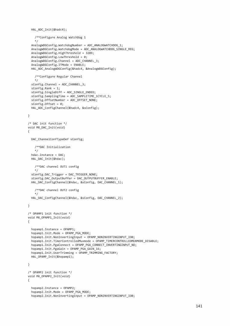
141
HAL_ADC_Init(&hadc4); /**Configure Analog WatchDog 1 */ AnalogWDGConfig.WatchdogNumber = ADC_ANALOGWATCHDOG_1; AnalogWDGConfig.WatchdogMode = ADC_ANALOGWATCHDOG_SINGLE_REG; AnalogWDGConfig.HighThreshold = 3289; AnalogWDGConfig.LowThreshold = 0; AnalogWDGConfig.Channel = ADC_CHANNEL_3; AnalogWDGConfig.ITMode = ENABLE; HAL_ADC_AnalogWDGConfig(&hadc4, &AnalogWDGConfig); /**Configure Regular Channel */ sConfig.Channel = ADC_CHANNEL_3; sConfig.Rank = 1; sConfig.SingleDiff = ADC_SINGLE_ENDED; sConfig.SamplingTime = ADC_SAMPLETIME_1CYCLE_5; sConfig.OffsetNumber = ADC_OFFSET_NONE; sConfig.Offset = 0; HAL_ADC_ConfigChannel(&hadc4, &sConfig); } /* DAC init function */ void MX_DAC_Init(void) { DAC_ChannelConfTypeDef sConfig; /**DAC Initialization */ hdac.Instance = DAC; HAL_DAC_Init(&hdac); /**DAC channel OUT1 config */ sConfig.DAC_Trigger = DAC_TRIGGER_NONE; sConfig.DAC_OutputBuffer = DAC_OUTPUTBUFFER_ENABLE; HAL_DAC_ConfigChannel(&hdac, &sConfig, DAC_CHANNEL_1); /**DAC channel OUT2 config */ HAL_DAC_ConfigChannel(&hdac, &sConfig, DAC_CHANNEL_2); } /* OPAMP1 init function */ void MX_OPAMP1_Init(void) { hopamp1.Instance = OPAMP1; hopamp1.Init.Mode = OPAMP_PGA_MODE; hopamp1.Init.NonInvertingInput = OPAMP_NONINVERTINGINPUT_IO0; hopamp1.Init.TimerControlledMuxmode = OPAMP_TIMERCONTROLLEDMUXMODE_DISABLE; hopamp1.Init.PgaConnect = OPAMP_PGA_CONNECT_INVERTINGINPUT_NO; hopamp1.Init.PgaGain = OPAMP_PGA_GAIN_16; hopamp1.Init.UserTrimming = OPAMP_TRIMMING_FACTORY; HAL_OPAMP_Init(&hopamp1); } /* OPAMP2 init function */ void MX_OPAMP2_Init(void) { hopamp2.Instance = OPAMP2; hopamp2.Init.Mode = OPAMP_PGA_MODE; hopamp2.Init.NonInvertingInput = OPAMP_NONINVERTINGINPUT_IO0;

142
hopamp2.Init.TimerControlledMuxmode = OPAMP_TIMERCONTROLLEDMUXMODE_DISABLE; hopamp2.Init.PgaConnect = OPAMP_PGA_CONNECT_INVERTINGINPUT_NO; hopamp2.Init.PgaGain = OPAMP_PGA_GAIN_16; hopamp2.Init.UserTrimming = OPAMP_TRIMMING_FACTORY; HAL_OPAMP_Init(&hopamp2); } /* TIM1 init function */ void MX_TIM1_Init(void) { TIM_ClockConfigTypeDef sClockSourceConfig; TIM_MasterConfigTypeDef sMasterConfig; TIM_BreakDeadTimeConfigTypeDef sBreakDeadTimeConfig; TIM_OC_InitTypeDef sConfigOC; htim1.Instance = TIM1; htim1.Init.Prescaler = 0; htim1.Init.CounterMode = TIM_COUNTERMODE_UP; htim1.Init.Period = 64035; htim1.Init.ClockDivision = TIM_CLOCKDIVISION_DIV1; htim1.Init.RepetitionCounter = 0; HAL_TIM_Base_Init(&htim1); sClockSourceConfig.ClockSource = TIM_CLOCKSOURCE_INTERNAL; HAL_TIM_ConfigClockSource(&htim1, &sClockSourceConfig); HAL_TIM_PWM_Init(&htim1); sMasterConfig.MasterOutputTrigger = TIM_TRGO_UPDATE; sMasterConfig.MasterOutputTrigger2 = TIM_TRGO2_RESET; sMasterConfig.MasterSlaveMode = TIM_MASTERSLAVEMODE_ENABLE; HAL_TIMEx_MasterConfigSynchronization(&htim1, &sMasterConfig); sBreakDeadTimeConfig.OffStateRunMode = TIM_OSSR_DISABLE; sBreakDeadTimeConfig.OffStateIDLEMode = TIM_OSSI_DISABLE; sBreakDeadTimeConfig.LockLevel = TIM_LOCKLEVEL_OFF; sBreakDeadTimeConfig.DeadTime = 45; sBreakDeadTimeConfig.BreakState = TIM_BREAK_ENABLE; sBreakDeadTimeConfig.BreakPolarity = TIM_BREAKPOLARITY_HIGH; sBreakDeadTimeConfig.BreakFilter = 0; sBreakDeadTimeConfig.Break2State = TIM_BREAK2_DISABLE; sBreakDeadTimeConfig.Break2Polarity = TIM_BREAK2POLARITY_HIGH; sBreakDeadTimeConfig.Break2Filter = 0; sBreakDeadTimeConfig.AutomaticOutput = TIM_AUTOMATICOUTPUT_DISABLE; HAL_TIMEx_ConfigBreakDeadTime(&htim1, &sBreakDeadTimeConfig); sConfigOC.OCMode = TIM_OCMODE_PWM1; sConfigOC.Pulse = 0; sConfigOC.OCPolarity = TIM_OCPOLARITY_HIGH; sConfigOC.OCNPolarity = TIM_OCNPOLARITY_HIGH; sConfigOC.OCFastMode = TIM_OCFAST_ENABLE; sConfigOC.OCIdleState = TIM_OCIDLESTATE_RESET; sConfigOC.OCNIdleState = TIM_OCNIDLESTATE_RESET; HAL_TIM_PWM_ConfigChannel(&htim1, &sConfigOC, TIM_CHANNEL_1); HAL_TIM_PWM_ConfigChannel(&htim1, &sConfigOC, TIM_CHANNEL_2); HAL_TIM_PWM_ConfigChannel(&htim1, &sConfigOC, TIM_CHANNEL_3); HAL_TIM_MspPostInit(&htim1); } /* TIM3 init function */ void MX_TIM3_Init(void) {

143
TIM_ClockConfigTypeDef sClockSourceConfig; TIM_MasterConfigTypeDef sMasterConfig; htim3.Instance = TIM3; htim3.Init.Prescaler = 2; htim3.Init.CounterMode = TIM_COUNTERMODE_UP; htim3.Init.Period = 57535; htim3.Init.ClockDivision = TIM_CLOCKDIVISION_DIV1; HAL_TIM_Base_Init(&htim3); sClockSourceConfig.ClockSource = TIM_CLOCKSOURCE_INTERNAL; HAL_TIM_ConfigClockSource(&htim3, &sClockSourceConfig); sMasterConfig.MasterOutputTrigger = TIM_TRGO_RESET; sMasterConfig.MasterSlaveMode = TIM_MASTERSLAVEMODE_DISABLE; HAL_TIMEx_MasterConfigSynchronization(&htim3, &sMasterConfig); } /* TIM4 init function */ void MX_TIM4_Init(void) { TIM_ClockConfigTypeDef sClockSourceConfig; TIM_MasterConfigTypeDef sMasterConfig; TIM_IC_InitTypeDef sConfigIC; htim4.Instance = TIM4; htim4.Init.Prescaler = 16; htim4.Init.CounterMode = TIM_COUNTERMODE_UP; htim4.Init.Period = 0; htim4.Init.ClockDivision = TIM_CLOCKDIVISION_DIV1; HAL_TIM_Base_Init(&htim4); sClockSourceConfig.ClockSource = TIM_CLOCKSOURCE_INTERNAL; HAL_TIM_ConfigClockSource(&htim4, &sClockSourceConfig); HAL_TIM_IC_Init(&htim4); sMasterConfig.MasterOutputTrigger = TIM_TRGO_OC1; sMasterConfig.MasterSlaveMode = TIM_MASTERSLAVEMODE_DISABLE; HAL_TIMEx_MasterConfigSynchronization(&htim4, &sMasterConfig); sConfigIC.ICPolarity = TIM_INPUTCHANNELPOLARITY_BOTHEDGE; sConfigIC.ICSelection = TIM_ICSELECTION_DIRECTTI; sConfigIC.ICPrescaler = TIM_ICPSC_DIV1; sConfigIC.ICFilter = 0; HAL_TIM_IC_ConfigChannel(&htim4, &sConfigIC, TIM_CHANNEL_1); HAL_TIM_IC_ConfigChannel(&htim4, &sConfigIC, TIM_CHANNEL_2); HAL_TIM_IC_ConfigChannel(&htim4, &sConfigIC, TIM_CHANNEL_3); } /* TIM16 init function */ void MX_TIM16_Init(void) { TIM_IC_InitTypeDef sConfigIC; htim16.Instance = TIM16; htim16.Init.Prescaler = 2; htim16.Init.CounterMode = TIM_COUNTERMODE_UP; htim16.Init.Period = 0; htim16.Init.ClockDivision = TIM_CLOCKDIVISION_DIV1; htim16.Init.RepetitionCounter = 0; HAL_TIM_Base_Init(&htim16);

144
HAL_TIM_IC_Init(&htim16); HAL_TIM_OnePulse_Init(&htim16, TIM_OPMODE_SINGLE); sConfigIC.ICPolarity = TIM_INPUTCHANNELPOLARITY_BOTHEDGE; sConfigIC.ICSelection = TIM_ICSELECTION_DIRECTTI; sConfigIC.ICPrescaler = TIM_ICPSC_DIV1; sConfigIC.ICFilter = 0; HAL_TIM_IC_ConfigChannel(&htim16, &sConfigIC, TIM_CHANNEL_1); } /* USART3 init function */ void MX_USART3_UART_Init(void) { huart3.Instance = USART3; huart3.Init.BaudRate = 38400; huart3.Init.WordLength = UART_WORDLENGTH_8B; huart3.Init.StopBits = UART_STOPBITS_1; huart3.Init.Parity = UART_PARITY_NONE; huart3.Init.Mode = UART_MODE_TX_RX; huart3.Init.HwFlowCtl = UART_HWCONTROL_NONE; huart3.Init.OverSampling = UART_OVERSAMPLING_16; huart3.Init.OneBitSampling = UART_ONE_BIT_SAMPLE_DISABLE; huart3.AdvancedInit.AdvFeatureInit = UART_ADVFEATURE_NO_INIT; HAL_UART_Init(&huart3); } /** Configure pins as * Analog * Input * Output * EVENT_OUT * EXTI */ void MX_GPIO_Init(void) { GPIO_InitTypeDef GPIO_InitStruct; /* GPIO Ports Clock Enable */ __HAL_RCC_GPIOF_CLK_ENABLE(); __HAL_RCC_GPIOA_CLK_ENABLE(); __HAL_RCC_GPIOB_CLK_ENABLE(); /*Configure GPIO pin : PB0 */ GPIO_InitStruct.Pin = GPIO_PIN_0; GPIO_InitStruct.Mode = GPIO_MODE_ANALOG; GPIO_InitStruct.Pull = GPIO_NOPULL; HAL_GPIO_Init(GPIOB, &GPIO_InitStruct); } /* USER CODE BEGIN 4 */ uint16_t getThrottlePwmVal(void){ temp = __HAL_TIM_GetCounter(&htim16); temp -= 16000; //16000 = 1ms which is the zero reading. temp = temp/5; //convert 0-16000 to 0-3200, suitable for PWM duty cycle values. return (temp); } void updateThrottle (void){ ThrottlePwmVal = getThrottlePwmVal();

145
//5% - 2.5% hystersis between motor start and stop if(ThrottlePwmVal > 160){ MC_StartMotor(); } if(ThrottlePwmVal < 80){ MC_StopMotor(); } } void filterThrottle(uint16_t currentValue){ uint32_t accumulator = 0; uint8_t index = 0; uint16_t dataArray[8] = 0; accumulator -= dataArray[index]; dataArray[index] = currentValue; accumulator += currentValue; index ++; if(index == 8){ index = 0; } MC_Set_Speed(accumulator / 8); } void setDacs(void){ uint32_t ch1Data = MC_GetMechSpeedRPM(); uint32_t ch2Data = MC_GetElSpeedHz(); HAL_DAC_SetValue(&hdac,DAC_CHANNEL_1,DAC_ALIGN_12B_R,ch1Data); HAL_DAC_Start(&hdac,DAC_CHANNEL_1); HAL_DAC_SetValue(&hdac,DAC_CHANNEL_2,DAC_ALIGN_12B_R,ch2Data); HAL_DAC_Start(&hdac,DAC_CHANNEL_2); } uint32_t getFilteredCurrent(uint32_t currentValue){ uint32_t accumulator = 0; uint8_t index = 0; uint16_t dataArray[8] = 0; accumulator -= dataArray[index]; dataArray[index] = currentValue; accumulator += currentValue; index ++; if(index == 8){ index = 0; } return (accumulator/8); } /* USER CODE END 4 */ #ifdef USE_FULL_ASSERT /** * @brief Reports the name of the source file and the source line number * where the assert_param error has occurred.

146
* @param file: pointer to the source file name * @param line: assert_param error line source number * @retval None */ void assert_failed(uint8_t* file, uint32_t line) { /* USER CODE BEGIN 6 */ /* User can add his own implementation to report the file name and line number, ex: printf("Wrong parameters value: file %s on line %d\r\n", file, line) */ /* USER CODE END 6 */ } #endif /** * @} */ /** * @} */ /************************ (C) COPYRIGHT STMicroelectronics *****END OF FILE****/
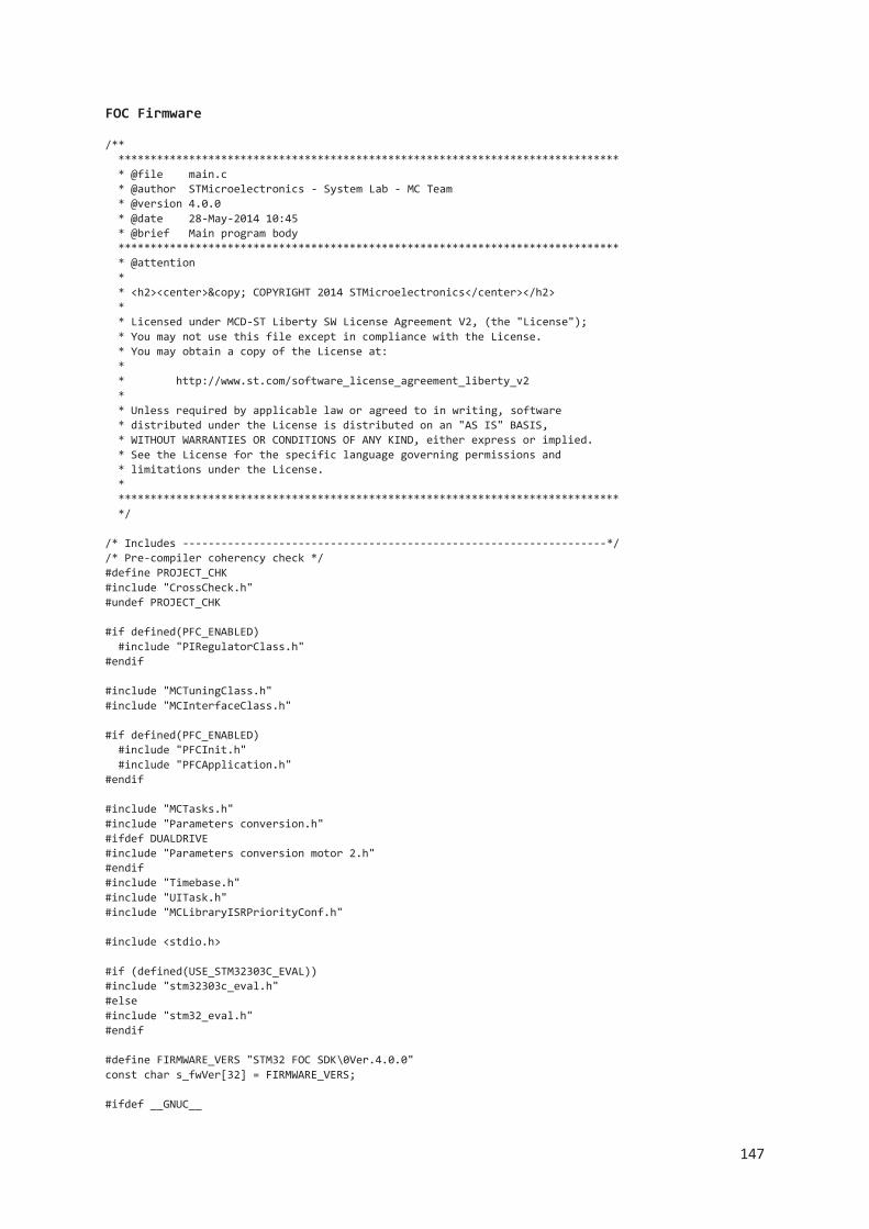
147
FOC Firmware /** ****************************************************************************** * @file main.c * @author STMicroelectronics - System Lab - MC Team * @version 4.0.0 * @date 28-May-2014 10:45 * @brief Main program body ****************************************************************************** * @attention * * <h2><center>© COPYRIGHT 2014 STMicroelectronics</center></h2> * * Licensed under MCD-ST Liberty SW License Agreement V2, (the "License"); * You may not use this file except in compliance with the License. * You may obtain a copy of the License at: * * http://www.st.com/software_license_agreement_liberty_v2 * * Unless required by applicable law or agreed to in writing, software * distributed under the License is distributed on an "AS IS" BASIS, * WITHOUT WARRANTIES OR CONDITIONS OF ANY KIND, either express or implied. * See the License for the specific language governing permissions and * limitations under the License. * ****************************************************************************** */ /* Includes ------------------------------------------------------------------*/ /* Pre-compiler coherency check */ #define PROJECT_CHK #include "CrossCheck.h" #undef PROJECT_CHK #if defined(PFC_ENABLED) #include "PIRegulatorClass.h" #endif #include "MCTuningClass.h" #include "MCInterfaceClass.h" #if defined(PFC_ENABLED) #include "PFCInit.h" #include "PFCApplication.h" #endif #include "MCTasks.h" #include "Parameters conversion.h" #ifdef DUALDRIVE #include "Parameters conversion motor 2.h" #endif #include "Timebase.h" #include "UITask.h" #include "MCLibraryISRPriorityConf.h" #include <stdio.h> #if (defined(USE_STM32303C_EVAL)) #include "stm32303c_eval.h" #else #include "stm32_eval.h" #endif #define FIRMWARE_VERS "STM32 FOC SDK\0Ver.4.0.0" const char s_fwVer[32] = FIRMWARE_VERS; #ifdef __GNUC__
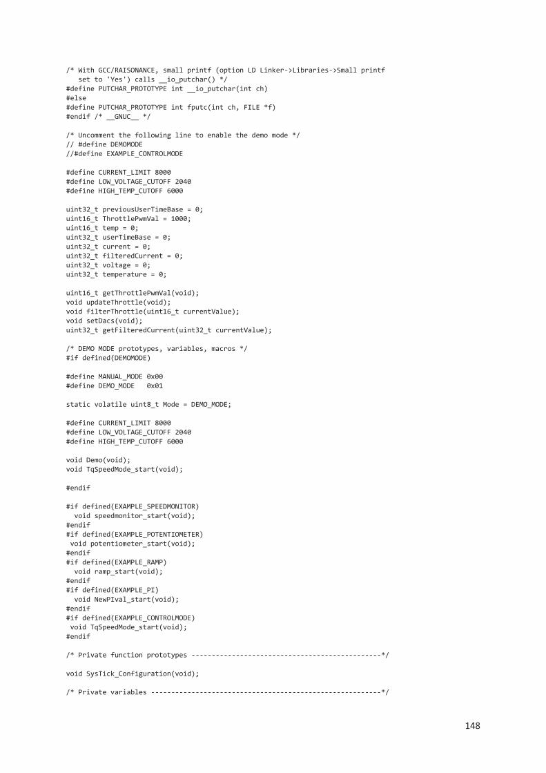
148
/* With GCC/RAISONANCE, small printf (option LD Linker->Libraries->Small printf set to 'Yes') calls __io_putchar() */ #define PUTCHAR_PROTOTYPE int __io_putchar(int ch) #else #define PUTCHAR_PROTOTYPE int fputc(int ch, FILE *f) #endif /* __GNUC__ */ /* Uncomment the following line to enable the demo mode */ // #define DEMOMODE //#define EXAMPLE_CONTROLMODE #define CURRENT_LIMIT 8000 #define LOW_VOLTAGE_CUTOFF 2040 #define HIGH_TEMP_CUTOFF 6000 uint32_t previousUserTimeBase = 0; uint16_t ThrottlePwmVal = 1000; uint16_t temp = 0; uint32_t userTimeBase = 0; uint32_t current = 0; uint32_t filteredCurrent = 0; uint32_t voltage = 0; uint32_t temperature = 0; uint16_t getThrottlePwmVal(void); void updateThrottle(void); void filterThrottle(uint16_t currentValue); void setDacs(void); uint32_t getFilteredCurrent(uint32_t currentValue); /* DEMO MODE prototypes, variables, macros */ #if defined(DEMOMODE) #define MANUAL_MODE 0x00 #define DEMO_MODE 0x01 static volatile uint8_t Mode = DEMO_MODE; #define CURRENT_LIMIT 8000 #define LOW_VOLTAGE_CUTOFF 2040 #define HIGH_TEMP_CUTOFF 6000 void Demo(void); void TqSpeedMode_start(void); #endif #if defined(EXAMPLE_SPEEDMONITOR) void speedmonitor_start(void); #endif #if defined(EXAMPLE_POTENTIOMETER) void potentiometer_start(void); #endif #if defined(EXAMPLE_RAMP) void ramp_start(void); #endif #if defined(EXAMPLE_PI) void NewPIval_start(void); #endif #if defined(EXAMPLE_CONTROLMODE) void TqSpeedMode_start(void); #endif /* Private function prototypes -----------------------------------------------*/ void SysTick_Configuration(void); /* Private variables ---------------------------------------------------------*/

149
CMCI oMCI[MC_NUM]; CMCT oMCT[MC_NUM]; uint32_t wConfig[MC_NUM] = {UI_CONFIG_M1,UI_CONFIG_M2}; /* Private macro -------------------------------------------------------------*/ /* Private variables ---------------------------------------------------------*/ /** * @brief Main program. * @param None * @retval None */ int main(void) { /*!< At this stage the microcontroller clock setting is already configured, this is done through SystemInit() function which is called from startup file (startup_stm32f10x_xx.s) before to branch to application main. To reconfigure the default setting of SystemInit() function, refer to system_stm32f10x.c file */ #if !defined(STM32F0XX) /*NVIC Priority group configuration. Default option is NVIC_PriorityGroup_3. */ NVIC_PriorityGroupConfig(NVIC_PriorityGroup_3); #endif /*MCInterface and MCTuning boot*/ MCboot(oMCI,oMCT); #if defined(PFC_ENABLED) PFC_Boot(oMCT[0],(CMCT)MC_NULL, (int16_t *)MC_NULL); #endif /*Systick configuration.*/ SysTick_Configuration(); /* Start here ***************************************************************/ /* GUI, this section is present only if LCD, DAC or serial communication is */ /* enabled. */ #if (defined(LCD_FUNCTIONALITY) | defined(DAC_FUNCTIONALITY) | defined(SERIAL_COMMUNICATION)) UI_TaskInit(UI_INIT_CFG,wConfig,MC_NUM,oMCI,oMCT,s_fwVer); #endif /* End here******************************************************************/ while(1) { #ifdef SERIAL_COMMUNICATION /* Start here ***********************************************************/ /* GUI, this section is present only if serial communication is enabled.*/ if (UI_SerialCommunicationTimeOutHasElapsed()) { // Send timeout message Exec_UI_IRQ_Handler(UI_IRQ_USART,3,0); // Flag 3 = Send timeout error*/ } /* End here**************************************************************/ #endif #ifdef LCD_FUNCTIONALITY /* Start here ***********************************************************/ /* GUI, this section is present only if LCD is enabled. */ if (UI_IdleTimeHasElapsed()) { UI_SetIdleTime(UI_TASK_OCCURENCE_TICKS); UI_LCDRefresh(); } /* End here**************************************************************/

150
#endif /******************************** EXAMPLE AREA ******************************/ #if defined(EXAMPLE_POTENTIOMETER) potentiometer_start(); #endif #if defined(EXAMPLE_RAMP) ramp_start(); #endif #if defined(EXAMPLE_PI) NewPIval_start(); #endif #if defined(EXAMPLE_CONTROLMODE) TqSpeedMode_start(); #endif #if defined(EXAMPLE_SPEEDMONITOR) speedmonitor_start(); #endif /*****************************************************************************/ //HIGH FREQUENCY TASKS (2000Hz) if(userTimeBase != previousUserTimeBase){ previousUserTimeBase = userTimeBase; setDacs(); current = MCI_GetCurrent(); filteredCurrent = getFilteredCurrent(current); if(filteredCurrent > CURRENT_LIMIT){ MC_StopMotor(); } //MEDIUN FREQUENCY TASKS (500Hz) if((userTimeBase % 4) == 0){ voltage = MC_GetVoltage(); if(voltage < LOW_VOLTAGE_CUTOFF){ MC_StopMotor(); } } //LOW FREQUENCY TASKS (50Hz) if(userTimeBase >= 40){ userTimeBase = 0; //reset timebase } updateThrottle(); filterThrottle(ThrottlePwmVal); //applies filtered throttle value to MC temperature = MC_GetTemperature(); if (temperature > HIGH_TEMP_CUTOFF){ MC_StopMotor(); } }

151
} } /** * @brief Configures the SysTick. * @param None * @retval None */ void SysTick_Configuration(void) { /* Setup SysTick Timer for 500 usec interrupts */ if (SysTick_Config((SystemCoreClock) / SYS_TICK_FREQUENCY)) { /* Capture error */ while (1); } NVIC_SetPriority(SysTick_IRQn, SYSTICK_PRIORITY); NVIC_SetPriority(PendSV_IRQn, PENDSV_PRIORITY); } #ifdef USE_FULL_ASSERT /** * @brief Reports the name of the source file and the source line number * where the assert_param error has occurred. * @param file: pointer to the source file name * @param line: assert_param error line source number * @retval None */ void assert_failed(uint8_t* file, uint32_t line) { /* User can add his own implementation to report the file name and line number, ex: printf("Wrong parameters value: file %s on line %d\r\n", file, line) */ /* Infinite loop */ while (1) { } } #endif uint16_t getThrottlePwmVal(void){ temp = TIM_GetCounterVal(1, 16); temp -= 16000; //16000 = 1ms which is the zero reading. temp = temp/10; //convert 0-16000 to 0-1600, suitable for PWM duty cycle values. return (temp); } void updateThrottle (void){ ThrottlePwmVal = getThrottlePwmVal(); //5% - 2.5% hystersis between motor start and stop if(ThrottlePwmVal > 160){ MC_StartMotor(); } if(ThrottlePwmVal < 80){ MC_StopMotor(); } } void filterThrottle(uint16_t currentValue){ uint32_t accumulator = 0;

152
uint8_t index = 0; uint16_t dataArray[8] = 0; extern uint16_t speed_target; accumulator -= dataArray[index]; dataArray[index] = currentValue; accumulator += currentValue; index ++; if(index == 8){ index = 0; } speed_target = (accumulator / 8); } void setDacs(void){ uint32_t ch1Data = MC_GetMechSpeedRPM(); uint32_t ch2Data = MC_GetElSpeedHz(); DAC_SetChannel1Data(DAC_Align_12b_R, ch1Data); DAC_SetChannel1Data(DAC_Align_12b_R, ch2Data); } uint32_t getFilteredCurrent(uint32_t currentValue){ uint32_t accumulator = 0; uint8_t index = 0; uint16_t dataArray[8] = 0; accumulator -= dataArray[index]; dataArray[index] = currentValue; accumulator += currentValue; index ++; if(index == 8){ index = 0; } return (accumulator/8); } /******************* (C) COPYRIGHT 2014 STMicroelectronics *****END OF FILE****/

153
/** ****************************************************************************** * @file TqSpeedMode.c * @author STMicroelectronics - System Lab - MC Team * @version 4.0.0 * @date 28-May-2014 10:45 * @brief This file shows how to start the motor with different ramp profile ***************************************************************************** * @attention * * <h2><center>© COPYRIGHT 2014 STMicroelectronics</center></h2> * * Licensed under MCD-ST Liberty SW License Agreement V2, (the "License"); * You may not use this file except in compliance with the License. * You may obtain a copy of the License at: * * http://www.st.com/software_license_agreement_liberty_v2 * * Unless required by applicable law or agreed to in writing, software * distributed under the License is distributed on an "AS IS" BASIS, * WITHOUT WARRANTIES OR CONDITIONS OF ANY KIND, either express or implied. * See the License for the specific language governing permissions and * limitations under the License. * ****************************************************************************** */ /* Includes ------------------------------------------------------------------*/ /* Pre-compiler coherency check */ #include "MC.h" #include "Timebase.h" #include "SpeednPosFdbkClass.h" #include "Parameters conversion.h" #ifdef DUALDRIVE #include "Parameters conversion motor 2.h" #endif /*********************** DEFINE for USER STATE MACHINE ***********************/ #define US_RESET 0x00 #define US_POSITIVE_RUN 0x01 #define US_STOP 0x02 #define US_RAMP 0x03 #define US_SPEED 0x04 #define COUNT_MAX_SEC 5 #define STOP_DURATION_SEC 10 #define COUNT_MAX (COUNT_MAX_SEC * USER_TIMEBASE_FREQUENCY_HZ) #define STOP_DURATION (STOP_DURATION_SEC * USER_TIMEBASE_FREQUENCY_HZ) #define USER_TIMEBASE_FREQUENCY_HZ 10 #define USER_TIMEBASE_OCCURENCE_TICKS (SYS_TICK_FREQUENCY/USER_TIMEBASE_FREQUENCY_HZ)-1u void TqSpeedMode_start(void); /* variables ---------------------------------------------------------*/ /*Create the CMCI local reference: CMCI oMCI*/ static CMCI oMCI; /*Create the CMCT local reference: CMCT oMCT*/ static CMCT oMCT; static uint8_t User_State = US_RESET; bool cmd_status = FALSE; static uint16_t UserCnt = 0; int16_t value_Speed_RPM = 0; uint16_t torque_value = 20; //Set the first value for the speed ramp uint16_t torque_duration = 1000; //Set the duration for first ramp uint16_t speed_threshold = 1000; //Set the second value for the speed ramp uint16_t speed_target = 1500; //Set the second value for the speed ramp

154
uint16_t speed_duration = 1000; //Set the duration for second ramp /*This is the main function to use in the main.c in order to start the current example */ void TqSpeedMode_start() { /* Get reference of MCI*/ oMCI = GetMCI(M1); /* Get reference of MCT*/ oMCT = GetMCT(M1); /*Get the CSPD instance of SpeednPosFdbk Class */ CSPD xCSPD = MCT_GetSpeednPosSensorMain(oMCT); if (TB_UserTimebaseHasElapsed()) { /* User defined code */ switch (User_State) { case US_RESET: { /* Next state */ /* This command sets what will be the first torque ramp after the MCI_StartMotor command. It requires as first parameter the oMCI[0], as second parameter is the value of motor torque reference at the end of the ramp and as third parameter the torque ramp duration in milliseconds. */ MCI_ExecTorqueRamp(oMCI, torque_value, torque_duration); /* This is a user command used to start the motor. The speed ramp shall be pre programmed before the command.*/ cmd_status = MCI_StartMotor(oMCI); /* It verifies if the command "MCI_StartMotor" is successfully executed otherwise it tries to restart the procedure */ if(cmd_status==FALSE) { User_State = US_RESET; // Command NOT executed } else User_State = US_SPEED; // Command executed UserCnt = 0; } break; case US_SPEED: { /* The function "GetAvrgMecSpeed01Hz(..)" returns the last computed average mechanical speed, expressed in 01Hz (tenth of Hertz) */ value_Speed_RPM = SPD_GetAvrgMecSpeed01Hz(xCSPD)*6; /* The following code controls if the speed target is reached otherwise it remains in current state machine state*/ if(value_Speed_RPM >=(speed_threshold-6)) { /* The speed target has been reached */ MCI_ExecSpeedRamp(oMCI, speed_target/6, speed_duration); UserCnt = 0; User_State = US_STOP; } } break; case US_STOP: { /* After the time "STOP_DURATION" the motor will be restarted */ if (UserCnt >= STOP_DURATION) { /* Next state */

155
/* This is a user command to stop the motor */ MCI_StopMotor(oMCI); User_State = US_RESET; UserCnt = 0; } else { UserCnt++; } } break; } TB_SetUserTimebaseTime(USER_TIMEBASE_OCCURENCE_TICKS); } } /******************* (C) COPYRIGHT 2014 STMicroelectronics *****END OF FILE****/

156
Appendix E- Bench Testing Minitab Data Analysis

157
Bench Testing – Data analysis output from Minitab
Bench tests were carried out using a test rig comprised of a driving motor coupled directly to a generator motor. A power monitor with data logging functionality was used to record the power data output of the generator motor and power input to the driving motor. The power input for the driving motor while controlled under Six-Step Control could then be compared to that of while controlled under FOC.
Generator motor
In order to make comparisons between the relative performance of the driving motor while driven under Six-Step Control and FOC, we must first establish that the load motor is able to provide a consistent and repeatable load. The power output of the generator motor controller was monitored for four separate scenarios of driving motor configurations. Each of those tests were analysed using the regression analysis function within Minitab statistical analysis software. A line of best fit was fitted to the individual datasets and compared for similarity.

158
Driving motor with Six-Step control at 22.2V
Line of best fit
Regression Analysis
Regression Analysis: 6Step Generator Power 22V [W] versus Speed[km/h]_1 Method Rows unused 1 Analysis of Variance Source DF Adj SS Adj MS F-Value P-Value Regression 1 4240162 4240162 130445.03 0.000 Speed[km/h]_1 1 4240162 4240162 130445.03 0.000 Error 154 5006 33 Lack-of-Fit 151 5004 33 52.43 0.004 Pure Error 3 2 1 Total 155 4245167 Model Summary S R-sq R-sq(adj) R-sq(pred) 5.70135 99.88% 99.88% 99.88% Coefficients Term Coef SE Coef T-Value P-Value VIF Constant -86.79 1.22 -71.17 0.000 Speed[km/h]_1 14.1972 0.0393 361.17 0.000 1.00
5040302010
600
500
400
300
200
100
0
Speed [km/h]
6Ste
p Ge
nera
tor P
ower
22V
[W]
Generator data with Six-Step control at 22.2V6Step Generator Power 22V [W] = -86.79 + 14.1972 Speed[km/h]
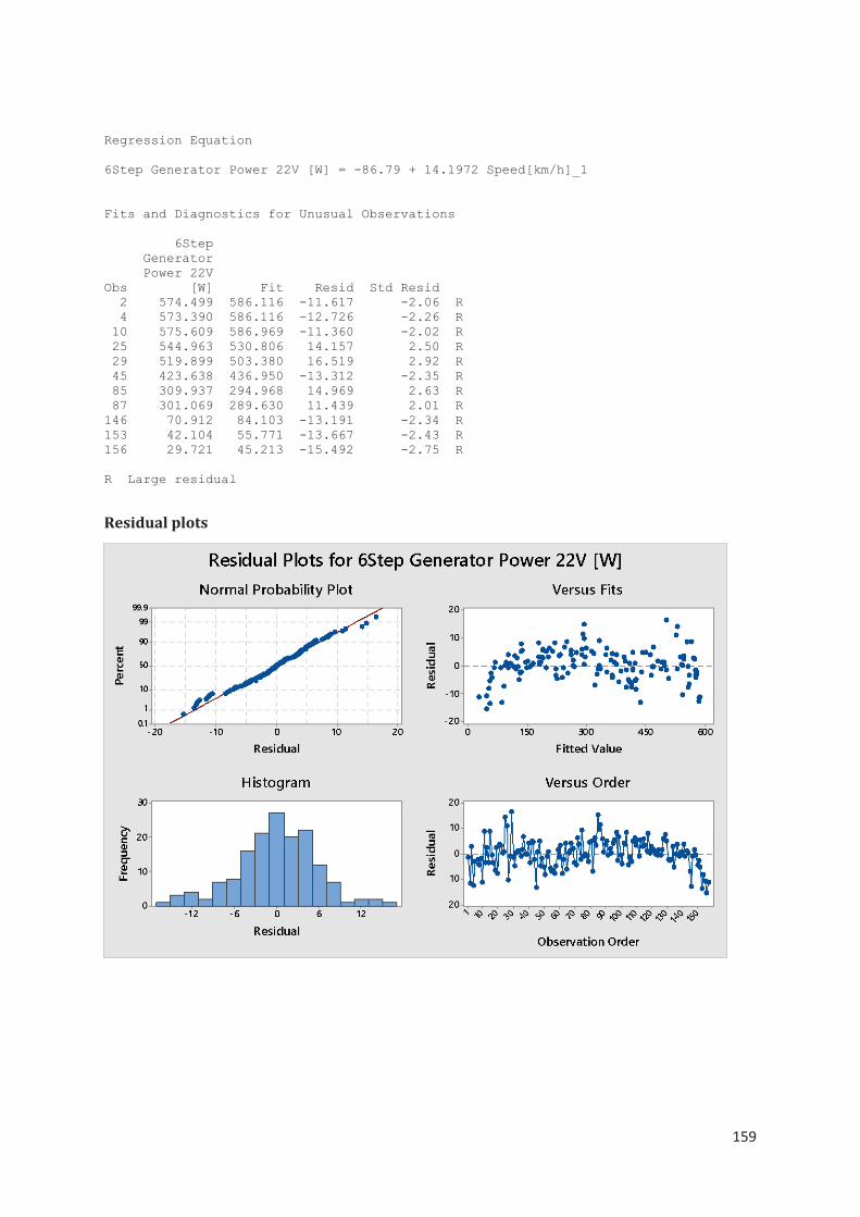
159
Regression Equation 6Step Generator Power 22V [W] = -86.79 + 14.1972 Speed[km/h]_1 Fits and Diagnostics for Unusual Observations 6Step Generator Power 22V Obs [W] Fit Resid Std Resid 2 574.499 586.116 -11.617 -2.06 R 4 573.390 586.116 -12.726 -2.26 R 10 575.609 586.969 -11.360 -2.02 R 25 544.963 530.806 14.157 2.50 R 29 519.899 503.380 16.519 2.92 R 45 423.638 436.950 -13.312 -2.35 R 85 309.937 294.968 14.969 2.63 R 87 301.069 289.630 11.439 2.01 R 146 70.912 84.103 -13.191 -2.34 R 153 42.104 55.771 -13.667 -2.43 R 156 29.721 45.213 -15.492 -2.75 R R Large residual
Residual plots

160
Driving motor with FOC at 22.2V
Line of best fit
Regression Analysis
Regression Analysis: FOC Generator Power 22V [W] versus Speed[km/h] Analysis of Variance Source DF Adj SS Adj MS F-Value P-Value Regression 1 4353309 4353309 237006.76 0.000 Speed[km/h] 1 4353309 4353309 237006.76 0.000 Error 227 4170 18 Lack-of-Fit 219 4123 19 3.21 0.039 Pure Error 8 47 6 Total 228 4357479 Model Summary S R-sq R-sq(adj) R-sq(pred) 4.28578 99.90% 99.90% 99.90% Coefficients Term Coef SE Coef T-Value P-Value VIF Constant -82.870 0.864 -95.92 0.000 Speed[km/h] 14.2713 0.0293 486.83 0.000 1.00 Regression Equation FOC Generator Power 22V [W] = -82.870 + 14.2713 Speed[km/h]
5040302010
600
500
400
300
200
100
0
Speed[km/h]
FOC
Gene
rato
r Pow
er 2
2V [W
]
Generator data with Six-Step control at 22.2VFOC Generator Power 22V [W] = -82.870 + 14.2713 Speed[km/h]
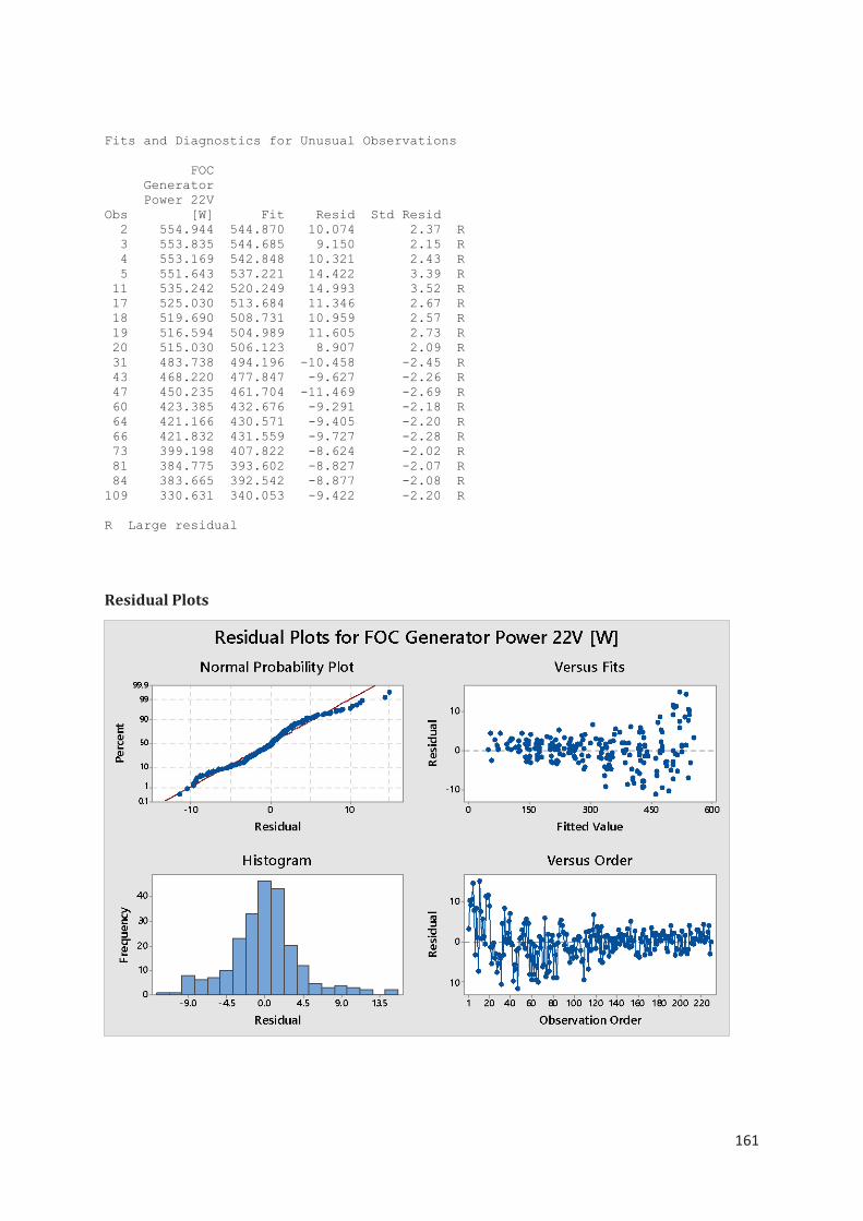
161
Fits and Diagnostics for Unusual Observations FOC Generator Power 22V Obs [W] Fit Resid Std Resid 2 554.944 544.870 10.074 2.37 R 3 553.835 544.685 9.150 2.15 R 4 553.169 542.848 10.321 2.43 R 5 551.643 537.221 14.422 3.39 R 11 535.242 520.249 14.993 3.52 R 17 525.030 513.684 11.346 2.67 R 18 519.690 508.731 10.959 2.57 R 19 516.594 504.989 11.605 2.73 R 20 515.030 506.123 8.907 2.09 R 31 483.738 494.196 -10.458 -2.45 R 43 468.220 477.847 -9.627 -2.26 R 47 450.235 461.704 -11.469 -2.69 R 60 423.385 432.676 -9.291 -2.18 R 64 421.166 430.571 -9.405 -2.20 R 66 421.832 431.559 -9.727 -2.28 R 73 399.198 407.822 -8.624 -2.02 R 81 384.775 393.602 -8.827 -2.07 R 84 383.665 392.542 -8.877 -2.08 R 109 330.631 340.053 -9.422 -2.20 R R Large residual
Residual Plots

162
Driving motor with Six-Step control at 30V
Line of best fit
Regression Analysis
Regression Analysis: 6Step Generator Power 30V [W] versus Speed[km/h]_3 Analysis of Variance Source DF Adj SS Adj MS F-Value P-Value Regression 1 7054841 7054841 107096.48 0.000 Speed[km/h]_3 1 7054841 7054841 107096.48 0.000 Error 139 9156 66 Lack-of-Fit 137 9039 66 1.13 0.586 Pure Error 2 117 59 Total 140 7063998 Model Summary S R-sq R-sq(adj) R-sq(pred) 8.11626 99.87% 99.87% 99.87% Coefficients Term Coef SE Coef T-Value P-Value VIF Constant -82.69 1.82 -45.48 0.000 Speed[km/h]_3 14.1203 0.0431 327.26 0.000 1.00 Regression Equation 6Step Generator Power 30V [W] = -82.69 + 14.1203 Speed[km/h]_3
70605040302010
900
800
700
600
500
400
300
200
100
0
Speed[km/h]_3
6Ste
p Ge
nera
tor P
ower
30V
[W]
Generator data with Six-Step control at 22.2V6Step Generator Power 30V [W] = -82.69 + 14.1203 Speed[km/h]

163
Fits and Diagnostics for Unusual Observations 6Step Generator Power 30V Obs [W] Fit Resid Std Resid 4 828.26 848.55 -20.29 -2.53 R 25 711.16 694.82 16.34 2.03 R 33 662.96 646.06 16.90 2.09 R 41 607.66 624.14 -16.48 -2.04 R 67 507.55 525.72 -18.17 -2.25 R 68 507.42 528.00 -20.58 -2.55 R 104 305.06 288.79 16.27 2.02 R 105 298.85 282.31 16.54 2.05 R 122 142.48 159.58 -17.10 -2.13 R R Large residual
Residual plots

164
Driving motor with FOC at 30V
Line of best fit
Regression analysis
Regression Analysis: FOC Generator Power 30V [W] versus Speed[km/h]_2 Analysis of Variance Source DF Adj SS Adj MS F-Value P-Value Regression 1 6183341 6183341 109850.62 0.000 Speed[km/h]_2 1 6183341 6183341 109850.62 0.000 Error 116 6529 56 Lack-of-Fit 113 6417 57 1.51 0.422 Pure Error 3 113 38 Total 117 6189870 Model Summary S R-sq R-sq(adj) R-sq(pred) 7.50258 99.89% 99.89% 99.89% Coefficients Term Coef SE Coef T-Value P-Value VIF Constant -73.17 1.89 -38.81 0.000 Speed[km/h]_2 13.9131 0.0420 331.44 0.000 1.00 Regression Equation FOC Generator Power 30V [W] = -73.17 + 13.9131 Speed[km/h]_2
70605040302010
900
800
700
600
500
400
300
200
100
0
Speed[km/h]_2
FOC
Gene
rato
r Pow
er 3
0V [W
]
Generator data with Six-Step control at 22.2VFOC Generator Power 30V [W] = -73.17 + 13.9131 Speed[km/h]

165
Fits and Diagnostics for Unusual Observations FOC Generator Power 30V Obs [W] Fit Resid Std Resid 2 816.47 834.02 -17.55 -2.37 R 12 832.71 813.56 19.15 2.58 R 13 827.74 810.55 17.19 2.32 R 17 800.49 781.90 18.59 2.50 R 23 774.70 752.43 22.27 3.00 R R Large residual
Residual plots
Summary of Individual model equations
The following equations show the line of best fit model for the individual datasets:
Six-Step at 22.2V: Generator power [W] = -86.79 + 14.1972 x Speed [km/h]
FOC at 22.2V: Generator power [W] = -82.87 + 14.2713 x Speed [km/h]
Six-Step at 30V: Generator power [W] = -82.69 + 14.1203 x Speed [km/h]
FOC at 30V: Generator power [W] = -73.17 + 13.9131 x Speed [km/h]

166
Overlaid on one plot
Additionally, the four data sets of the individual driving motor configurations were plotted on a single chart to give a visual indication of the similarity of the datasets:
Combined Generator Data Model
The four separate generator test runs were deemed to be sufficiently similar in terms of consistency and repeatability. The four datasets were combined into one and a regression analysis was conducted on the combined data:
706050403020100
900
800
700
600
500
400
300
200
100
0
Speed [km/h]
Gene
rato
r Pow
er [W
]
6Step Generator Power 22V [W] * Speed[km/h]_1FOC Generator Power 22V [W] * Speed[km/h]6Step Generator Power 30V [W] * Speed[km/h]_3FOC Generator Power 30V [W] * Speed[km/h]_2
Variable
Combined Generator Data

167
Line of best fit
Regression analysis
Regression Analysis: Generator power [W] all data versus Speed [km/h] all data Method Rows unused 1 Analysis of Variance Source DF Adj SS Adj MS F-Value P-Value Regression 1 25802001 25802001 585755.96 0.000 Speed [km/h] all data 1 25802001 25802001 585755.96 0.000 Error 636 28015 44 Lack-of-Fit 599 25644 43 0.67 0.968 Pure Error 37 2371 64 Total 637 25830016 Model Summary S R-sq R-sq(adj) R-sq(pred) 6.63695 99.89% 99.89% 99.89% Coefficients Term Coef SE Coef T-Value P-Value VIF Constant -80.592 0.662 -121.72 0.000 Speed [km/h] all data 14.0940 0.0184 765.35 0.000 1.00 Regression Equation
706050403020100
900
800
700
600
500
400
300
200
100
0
Speed [km/h] all data
Gene
rato
r pow
er [W
] all
data
Generator data with Six-Step control at 22.2VGenerator power [W] = -80.592 + 14.0940 Speed [km/h]
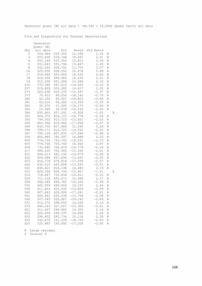
168
Generator power [W] all data = -80.592 + 14.0940 Speed [km/h] all data Fits and Diagnostics for Unusual Observations Generator power [W] Obs all data Fit Resid Std Resid 2 554.944 539.350 15.594 2.35 R 3 553.835 539.168 14.667 2.21 R 4 553.169 537.354 15.815 2.39 R 5 551.643 531.796 19.847 2.99 R 8 542.546 528.791 13.755 2.07 R 16 525.030 508.552 16.478 2.49 R 17 519.690 503.660 16.030 2.42 R 18 516.594 499.964 16.630 2.51 R 19 515.030 501.084 13.946 2.10 R 232 573.390 587.415 -14.025 -2.12 R 257 519.899 505.282 14.617 2.20 R 273 423.638 439.335 -15.697 -2.37 R 373 70.912 89.054 -18.142 -2.74 R 380 42.104 60.927 -18.823 -2.84 R 381 43.010 56.560 -13.550 -2.05 R 382 35.472 51.645 -16.173 -2.44 R 383 15.948 32.478 -16.530 -2.50 R 384 830.665 837.591 -6.926 -1.05 X 385 809.375 826.153 -16.778 -2.54 R 392 799.302 812.723 -13.421 -2.03 R 393 802.306 819.964 -17.658 -2.67 R 394 832.705 817.665 15.040 2.28 R 396 798.171 812.723 -14.552 -2.20 R 397 790.139 807.835 -17.696 -2.68 R 399 800.485 785.597 14.888 2.25 R 400 774.734 792.765 -18.031 -2.73 R 405 774.700 755.740 18.960 2.87 R 408 733.040 749.818 -16.778 -2.54 R 417 689.635 702.965 -13.330 -2.01 R 421 664.213 681.192 -16.979 -2.56 R 422 654.088 667.690 -13.602 -2.05 R 423 659.779 676.818 -17.039 -2.57 R 425 630.515 643.808 -13.293 -2.01 R 502 830.621 816.138 14.483 2.19 R 503 826.186 836.793 -10.607 -1.61 X 519 718.847 732.858 -14.011 -2.12 R 524 711.159 695.475 15.684 2.37 R 528 668.282 684.782 -16.500 -2.49 R 532 662.959 646.804 16.155 2.44 R 538 611.803 625.632 -13.829 -2.09 R 540 607.663 624.924 -17.261 -2.61 R 541 606.481 620.239 -13.758 -2.08 R 566 507.545 526.687 -19.142 -2.89 R 571 512.275 498.055 14.220 2.14 R 573 494.243 507.567 -13.324 -2.01 R 601 311.267 296.962 14.305 2.16 R 602 305.059 290.197 14.862 2.24 R 603 298.852 283.734 15.118 2.28 R 620 142.479 161.234 -18.755 -2.83 R 625 125.883 143.092 -17.209 -2.60 R R Large residual X Unusual X
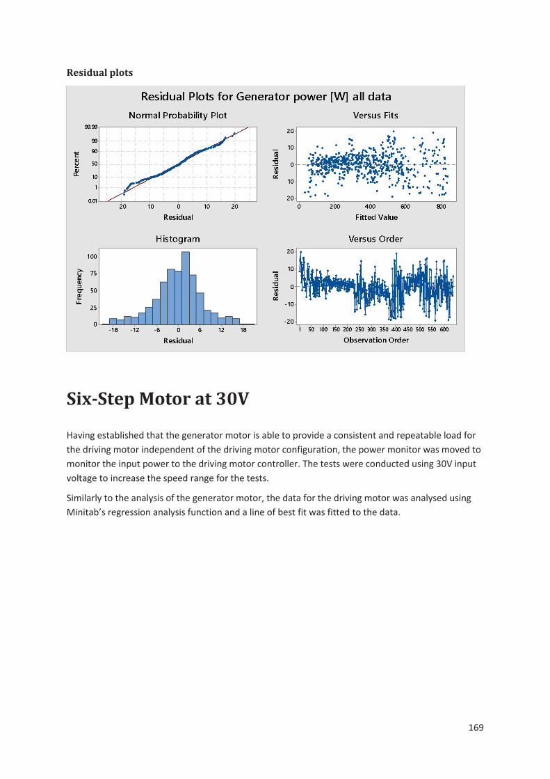
169
Residual plots
Six-Step Motor at 30V
Having established that the generator motor is able to provide a consistent and repeatable load for the driving motor independent of the driving motor configuration, the power monitor was moved to monitor the input power to the driving motor controller. The tests were conducted using 30V input voltage to increase the speed range for the tests.
Similarly to the analysis of the generator motor, the data for the driving motor was analysed using Minitab’s regression analysis function and a line of best fit was fitted to the data.

170
Line of best Fit
Regression Analysis
Regression Analysis: 6Step Motor Power [W] 30V versus Speed [km/h] 30V 6Step Analysis of Variance Source DF Adj SS Adj MS F-Value P-Value Regression 1 8941809 8941809 50899.90 0.000 Speed [km/h] 30V 6Step 1 8941809 8941809 50899.90 0.000 Error 121 21257 176 Total 122 8963065 Model Summary S R-sq R-sq(adj) R-sq(pred) 13.2542 99.76% 99.76% 99.75% Coefficients Term Coef SE Coef T-Value P-Value VIF Constant 95.99 3.03 31.69 0.000 Speed [km/h] 30V 6Step 16.0296 0.0711 225.61 0.000 1.00 Regression Equation 6Step Motor Power [W] 30V = 95.99 + 16.0296 Speed [km/h] 30V 6Step
70605040302010
1100
1000
900
800
700
600
500
400
300
200
Speed [km/h] 30V 6Step
6Ste
p M
otor
Pow
er [W
] 30V
Motor Data under Six-Step control at 30VMotor Power [W] 30V = 95.99 + 16.0296 Speed [km/h]

171
Fits and Diagnostics for Unusual Observations 6Step Motor Obs Power [W] 30V Fit Resid Std Resid 1 1143.86 1110.90 32.96 2.52 R 6 1144.15 1114.19 29.96 2.29 R 13 1144.15 1114.47 29.68 2.27 R 25 1027.00 1054.32 -27.32 -2.08 R 26 1022.00 1049.21 -27.21 -2.07 R R Large residual
Residual plot

172
FOC Motor at 30V
Line of best Fit
Regression Analysis
Regression Analysis: FOC Motor Power [W] 30V versus Speed [km/h] 30V FOC Analysis of Variance Source DF Adj SS Adj MS F-Value P-Value Regression 1 8189895 8189895 203871.61 0.000 Speed [km/h] 30V FOC 1 8189895 8189895 203871.61 0.000 Error 131 5263 40 Total 132 8195158 Model Summary S R-sq R-sq(adj) R-sq(pred) 6.33812 99.94% 99.94% 99.93% Coefficients Term Coef SE Coef T-Value P-Value VIF Constant 79.29 1.33 59.72 0.000 Speed [km/h] 30V FOC 16.3601 0.0362 451.52 0.000 1.00 Regression Equation FOC Motor Power [W] 30V = 79.29 + 16.3601 Speed [km/h] 30V FOC
605040302010
1100
1000
900
800
700
600
500
400
300
200
Speed [km/h] 30V FOC
FOC
Mot
or P
ower
[W] 3
0V
Motor Data under FOC at 30VMotor Power [W] 30V = 79.29 + 16.3601 Speed [km/h]
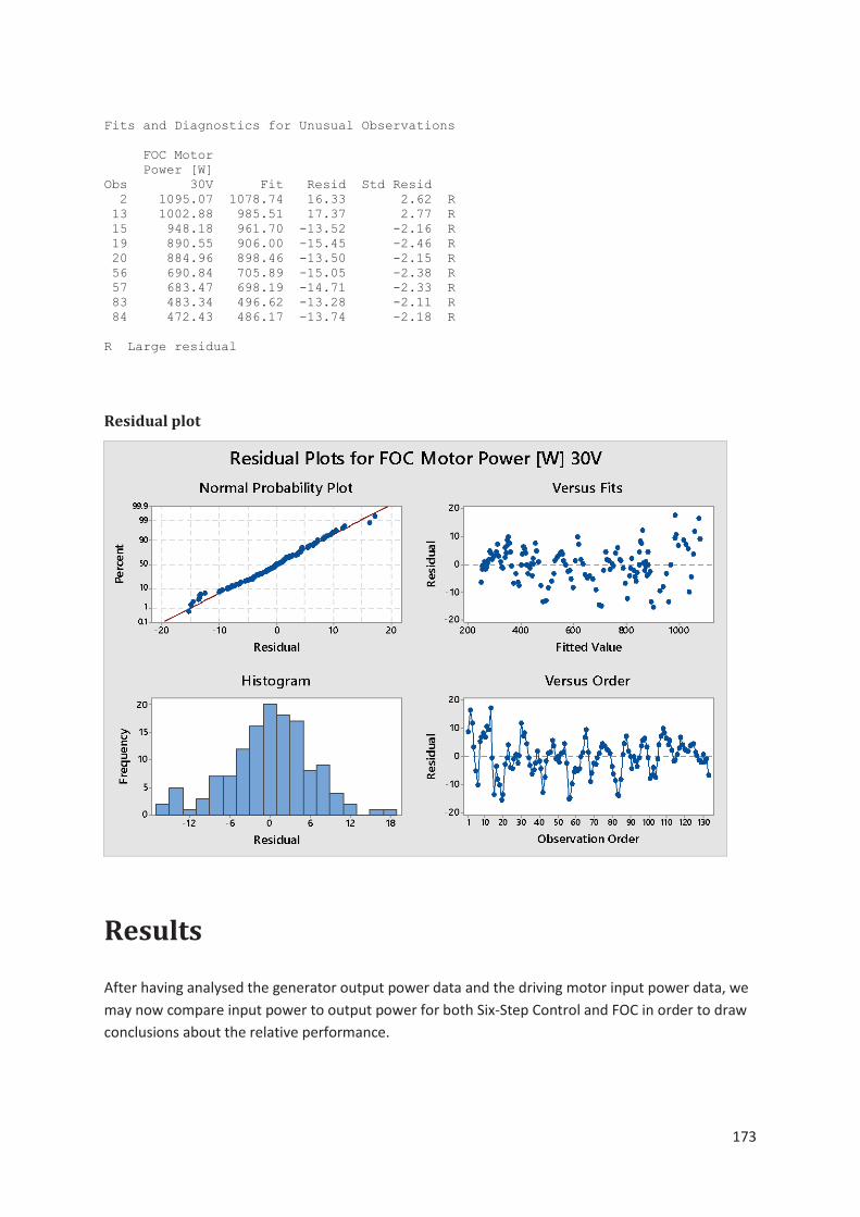
173
Fits and Diagnostics for Unusual Observations FOC Motor Power [W] Obs 30V Fit Resid Std Resid 2 1095.07 1078.74 16.33 2.62 R 13 1002.88 985.51 17.37 2.77 R 15 948.18 961.70 -13.52 -2.16 R 19 890.55 906.00 -15.45 -2.46 R 20 884.96 898.46 -13.50 -2.15 R 56 690.84 705.89 -15.05 -2.38 R 57 683.47 698.19 -14.71 -2.33 R 83 483.34 496.62 -13.28 -2.11 R 84 472.43 486.17 -13.74 -2.18 R R Large residual
Residual plot
Results
After having analysed the generator output power data and the driving motor input power data, we may now compare input power to output power for both Six-Step Control and FOC in order to draw conclusions about the relative performance.
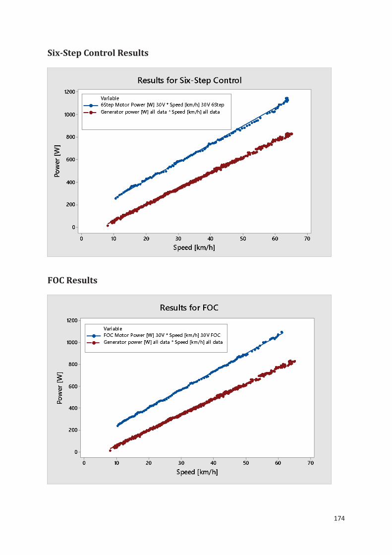
174
Six-Step Control Results
FOC Results

175
Six-Step Control and FOC results overlaid
Plotting the data series for both Six-Step Control and FOC driving motor configurations as well as the generator output power series on the same chart shows small differences in the required input power to drive the load.
Using actual data points

176
Using fitted equations
Power Consumed
Using the line of best fit equations, we can calculate how much power is consumed in the system (the difference in input power and output power). We can clearly see that the FOC implementation had lower power consumption than that of the Six-Step Control implementation for speeds below 50km/h. Above that speed, it appears that the Six-Step control implementation consumes less power.
70605040302010
1200
1000
800
600
400
200
0
Speed [km/h]
Powe
r [W
]
Power in [W] 6StepPower in [W] FOCPower out [W]
Variable
Six-Step, FOC, and Generated Power fitted lines
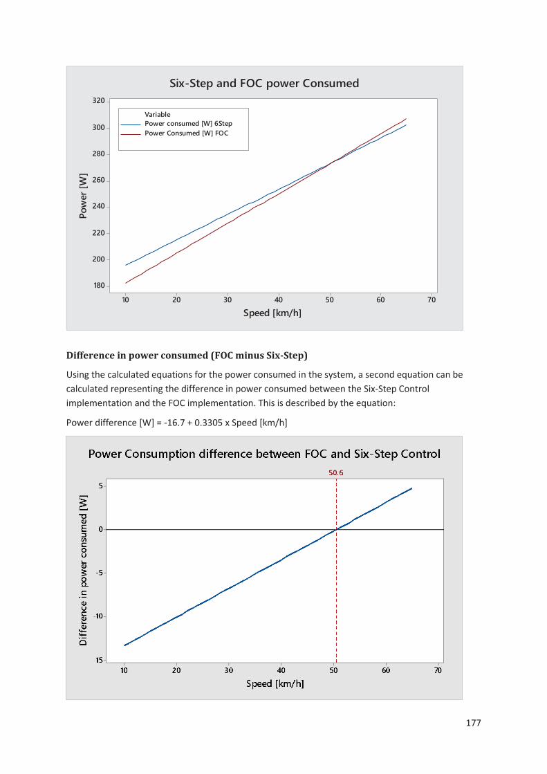
177
Difference in power consumed (FOC minus Six-Step)
Using the calculated equations for the power consumed in the system, a second equation can be calculated representing the difference in power consumed between the Six-Step Control implementation and the FOC implementation. This is described by the equation:
Power difference [W] = -16.7 + 0.3305 x Speed [km/h]
70605040302010
320
300
280
260
240
220
200
180
Speed [km/h]
Powe
r [W
]
Power consumed [W] 6StepPower Consumed [W] FOC
Variable
Six-Step and FOC power Consumed
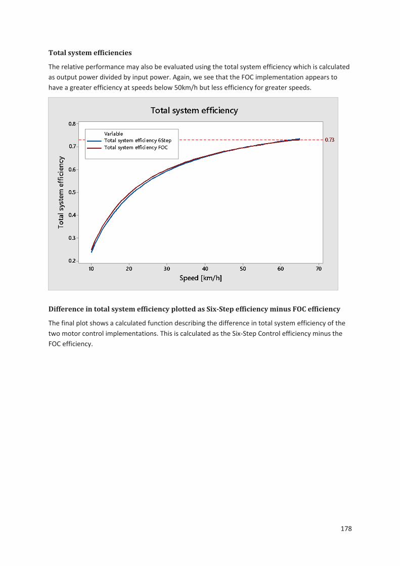
178
Total system efficiencies
The relative performance may also be evaluated using the total system efficiency which is calculated as output power divided by input power. Again, we see that the FOC implementation appears to have a greater efficiency at speeds below 50km/h but less efficiency for greater speeds.
Difference in total system efficiency plotted as Six-Step efficiency minus FOC efficiency
The final plot shows a calculated function describing the difference in total system efficiency of the two motor control implementations. This is calculated as the Six-Step Control efficiency minus the FOC efficiency.
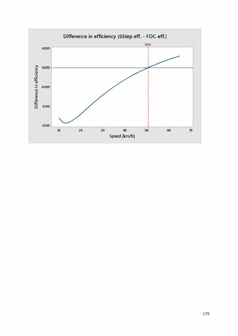
179

180
Appendix F - On-road Testing Data Analysis

181
On-road Testing Results
On road tests were carried out in order to evaluate the relative performance of Six-Step Control and FOC motor control techniques in the real world application. The motor controllers were fitted to the electric skateboard prototype and a power monitor with data logging functionality was used to record data for power input to one of the two motor controllers.
Range and Efficiency Tests
A test was designed to evaluate the relative range achievable and efficiency of the electric skateboard prototype when driven under Six-Step Control and FOC. The test involved travelling over a fixed distance, final speed, acceleration, and deceleration, as near as practicable.
First Repeat Test
The first test was carried out using a single battery charge; the test for Six-Step Control was performed directly after the test for FOC without charging the battery. Two return runs of the test route were completed for each test.
Speed Profiles
Six-Step speed profile:
The waiting times between passes of the test route were removed to give:

182
Statistics:
Metric Value Units Total capacity used 2412 mAh Total Distance travelled 4.108 km Start voltage 23.82 V Average voltage 23.24117 V Total energy used 56.6656 Wh Efficiency 13.79396 Wh/km Average speed 32.64636 km/h Battery capacity 444 Wh Range prediction 32.18799 km
The same test was carried out for FOC to give the following speed profile:
With waiting times removed:

183
Statistics:
Metric Value Units Total capacity used 2452 mAh Total Distance travelled 4.108 km Start voltage 24.53 V Average voltage 23.81284 V Total energy used 58.86342 Wh Efficiency 14.32897 Wh/km Average speed 32.68243 km/h Battery capacity 444 Wh Range prediction 30.98617 km
Second Repeat Test
The second test was carried out using a fully charged battery for each of the two test runs. Three return trips of the test route were completed.
Speed Profiles
Six Step speed profile:
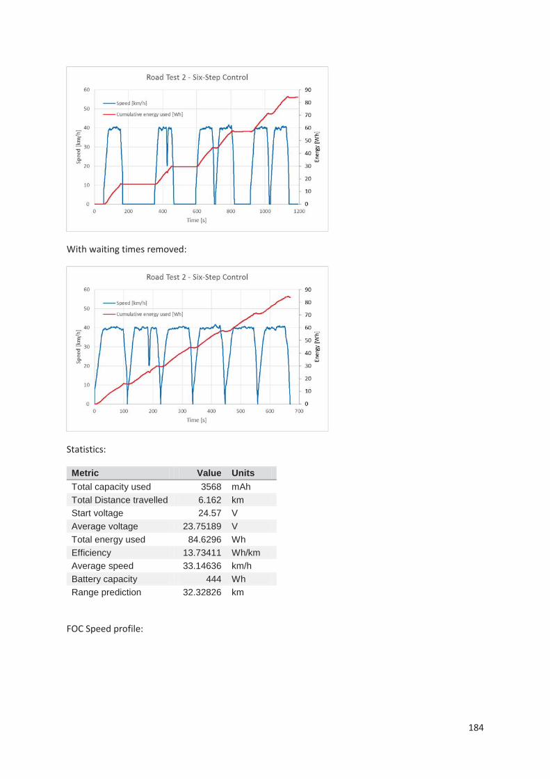
184
With waiting times removed:
Statistics:
Metric Value Units Total capacity used 3568 mAh Total Distance travelled 6.162 km Start voltage 24.57 V Average voltage 23.75189 V Total energy used 84.6296 Wh Efficiency 13.73411 Wh/km Average speed 33.14636 km/h Battery capacity 444 Wh Range prediction 32.32826 km
FOC Speed profile:

185
With waiting times removed:
Statistics:
Metric Value Units Total capacity used 3088 mAh Total Distance travelled 6.162 km Start voltage 24.5 V Average voltage 23.66251 V Total energy used 73.70838 Wh Efficiency 11.96176 Wh/km Average speed 31.84953 km/h Battery capacity 444 Wh Range prediction 37.11828 km
Third Repeat Test
The third test was carried out using a fully charged battery for each of the two test runs. Three return trips of the test route were completed.

186
Speed Profiles
Six-Step Speed Profile:
With waiting times removed:
Statistics:
Metric Value Units Total capacity used 3066 mAh Total Distance travelled 6.162 km Start voltage 24.52 V Average voltage 23.73917 V Total energy used 73.12384 Wh Efficiency 11.8669 Wh/km Average speed 33.18355 km/h Battery capacity 444 Wh Range prediction 37.41499 km
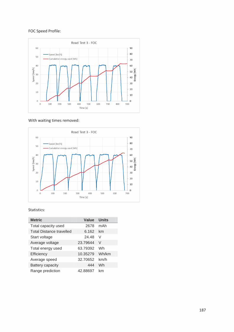
187
FOC Speed Profile:
With waiting times removed:
Statistics:
Metric Value Units Total capacity used 2678 mAh Total Distance travelled 6.162 km Start voltage 24.48 V Average voltage 23.79644 V Total energy used 63.79392 Wh Efficiency 10.35279 Wh/km Average speed 32.70652 km/h Battery capacity 444 Wh Range prediction 42.88697 km

188
Range and efficiency test summary
The third test, “Road Test 3” was identified as the most similar test between the Six-Step Control test run and the FOC test run as there were no interruptions due to pedestrians, cyclists, etc. The speed profiles for Six-Step Control and FOC are shown below overlaid on one plot:
We can see that similarity in speed profiles between the Six-Step Control test and FOC test was achieved.
The summary of data from the three repeated tests is given in the table below:
Test Number Average Speed [km/h]
Start Battery Voltage [V]
Energy Consumption [Wh/km]
Calculated Range [km]
Six-Step Control
Test 1 32.65 23.82 13.65 32.19 Test 2 33.15 24.57 13.73 32.33 Test 3 33.18 24.52 11.87 37.41 Average 32.99 24.30 13.08 33.98
Field Oriented Control
Test 1 32.68 24.53 14.33 30.99 Test 2 31.85 24.50 11.96 37.12 Test 3 32.71 24.48 10.35 42.89 Average 32.41 24.50 12.21 37.00
We can also see that all of the test runs were able to be carried out at a similar average speed.
Performance Test
Another on-road test was designed to evaluate the relative performance achieved from driving the motors under Six-Step Control and FOC. The test involved accelerating at the maximum current limit of 60A up to the maximum speed, then re-gen breaking at the maximum current limit to a complete stop.
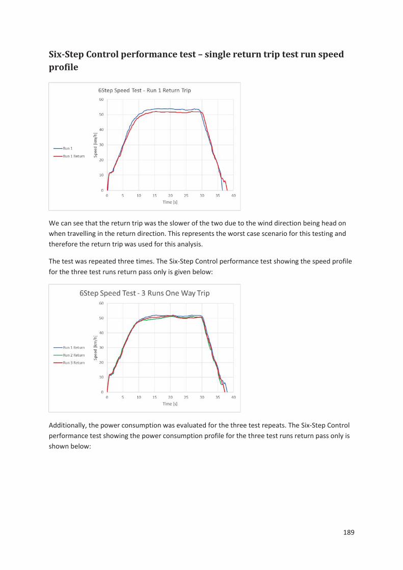
189
Six-Step Control performance test – single return trip test run speed profile
We can see that the return trip was the slower of the two due to the wind direction being head on when travelling in the return direction. This represents the worst case scenario for this testing and therefore the return trip was used for this analysis.
The test was repeated three times. The Six-Step Control performance test showing the speed profile for the three test runs return pass only is given below:
Additionally, the power consumption was evaluated for the three test repeats. The Six-Step Control performance test showing the power consumption profile for the three test runs return pass only is shown below:

190
Six-Step Control Statistics
Metric Value Units Run 1 max speed 53.97232 km/h Run 1 return max 51.95046 km/h Run 2 return max 51.06484 km/h Run 3 return max 51.96849 km/h Run1 return max power 2166.276 W Run2 return max power 2154.68 W Run3 return max power 2147.18 W Run1 return min power -1114.19 W Run2 return min power -1081.54 W Run3 return min power -1086.99 W Run 1 return 0-40km/h 7.5 s Run 2 return 0-40km/h 7.25 s Run 3 return 0-40km/h 7.5 s Run 1 return 40-0 km/h 6.25 s Run 2 return 40-0 km/h 6 s Run 3 return 40-0 km/h 6 s
FOC performance test – single return trip test run speed profile
The same tests were carried out using the FOC technique to drive the motors.

191
Again the return trip was the slower of the two due to the wind direction being head on when travelling in the return direction. This represents the worst case scenario for this testing and therefore the return trip was used for this analysis.
The test was repeated three times. The FOC performance test showing the speed profile for the three test runs return pass only (worst case scenario) is given below:
Again, the power consumption was evaluated for these tests. The FOC performance test showing the power consumption profile for the three test runs return pass only is shown below:
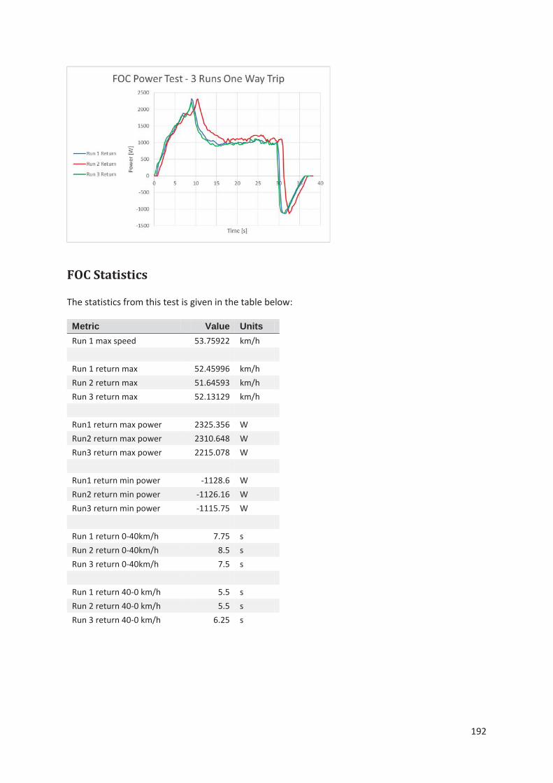
192
FOC Statistics
The statistics from this test is given in the table below:
Metric Value Units Run 1 max speed 53.75922 km/h Run 1 return max 52.45996 km/h Run 2 return max 51.64593 km/h Run 3 return max 52.13129 km/h Run1 return max power 2325.356 W Run2 return max power 2310.648 W Run3 return max power 2215.078 W Run1 return min power -1128.6 W Run2 return min power -1126.16 W Run3 return min power -1115.75 W Run 1 return 0-40km/h 7.75 s Run 2 return 0-40km/h 8.5 s Run 3 return 0-40km/h 7.5 s Run 1 return 40-0 km/h 5.5 s Run 2 return 40-0 km/h 5.5 s Run 3 return 40-0 km/h 6.25 s

193
Summary
The following table summarises the results from the performance test for the case where the motors are driven under Six-Step Control and FOC:
Run number Max Speed [km/h]
Max Power [W]
Max Regen Power [W]
Acceleration 0 - 40 km/h [s]
Deceleration 40 - 0 km/h [s]
Six-Step Control
Run1 51.95 2166 -1114 7.5 6.25 Run2 51.06 2155 -1082 7.25 6 Run3 51.99 2147 -1087 7.5 6 Average 51.67 2156 -1094 7.42 6.08
Field Oriented Control
Run1 52.46 2325 -1129 7.75 5.5 Run2 51.65 2311 -1126 8.5 5.5 Run3 52.13 2215 -1116 7.5 6.25 Average 52.08 2284 -1124 7.92 5.75