motivic zeta functions for prehomogeneous vector spaces and
TRANSCRIPT
F. LoeserNagoya Math. J.Vol. 171 (2003), 85–105
MOTIVIC ZETA FUNCTIONS FOR
PREHOMOGENEOUS VECTOR SPACES AND
CASTLING TRANSFORMATIONS
FRANCOIS LOESER
Abstract. We study the behaviour of motivic zeta functions of prehomoge-neous vector spaces under castling transformations. In particular we deducehow the motivic Milnor fibre and the Hodge spectrum at the origin behaveunder such transformations.
§1. Introduction
1.1. Let us recall the classification of irreducible regular prehomoge-
neous vector spaces due to Sato and Kimura [18]. A prehomogeneous vector
space over a field k [18] consists of the datum (G,X) of a connected linear
k-algebraic group G together with a linear representation ρ of G on a finite
dimensional affine space X = Amk over k having a Zariski dense G-orbit.
The complement of the Zariski dense G-orbit is called the singular locus
of the prehomogeneous vector space. When X is an irreducible G-module,
one says the prehomogeneous vector space (G,X) is irreducible.
One may find a general definition of regular prehomogeneous vector
spaces in [18], which, when the group G is reductive, is equivalent to the
condition that the singular locus is an hypersurface. From now on, except
for Section 7, we shall always assume the group G to be reductive. When
(G,X) is an irreducible regular prehomogeneous vector space, the singular
locus is an irreducible hypersurface f = 0 in X.
In the theory of Sato and Kimura, a fundamental role is played by
castling transforms, which are defined as follows.
Let G be a connected reductive k-algebraic group and ρ be a linear
representation of G on Amk . Write m = r1 + r2. Then set X1 = Mm,r1
and
let G × SLr1act on X1 by
ρ1(g, g1)x1 = ρ(g)x1tg1.
Received November 27, 2001.2000 Mathematics Subject Classification: 11S90, 14L30, 32S55; 14L24.
86 F. LOESER
Similarly set X2 = Mm,r2and let G × SLr2
act on X2 by
ρ2(g, g2)x2 = tρ(g)−1x2tg2.
Assume Gj = Imρj is an irreducible regular prehomogeneous vector space
for j = 1, 2 with singular locus the irreducible hypersurface fj = 0. In this
case one says that the prehomogeneous vector spaces (G1, X1) and (G2, X2)
are related by a castling transformation. Furthermore, cf. 4.1, f1 and f2
are homogeneous polynomials whose degrees satisfy deg fj = rjd, for some
integer d. We shall say that two irreducible regular prehomogeneous vector
spaces over k are equivalent if, up to isomorphism, they may be included
in a finite chain of irreducible regular prehomogeneous vector spaces whose
consecutive terms are related by a castling transform. In each equivalence
class there is a unique prehomogeneous vector space with dimX minimal.
Such an object is called reduced in the terminology of Sato and Kimura.
When k is algebraically closed of characteristic zero, the set of all reduced
irreducible regular prehomogeneous vector spaces has been divided into 29
types by Sato and Kimura [17]. If k is of characteristic zero and one restricts
to k-split groups, then the absolute classification restricts to a relative one.
1.2. Thus, if one wants to compute the value of some invariant for ir-
reducible regular prehomogeneous vector spaces, it is enough: a) to under-
stand the behaviour of the invariant under castling transformations; b) to
compute the invariant explicitly for reduced prehomogeneous vector spaces.
For instance, when k = C, if one denotes by bj the b-function of fj, we have
the following relation due to Shintani (cf. [11]):
(1.2.1) b2(s)∏
1≤i≤r1
∏
0≤j<d
(s +
(i + j)
d
)= b1(s)
∏
1≤i≤r2
∏
0≤j<d
(s +
(i + j)
d
),
and the b-functions of all 29 types, except for one, have been tabulated by
Kimura in [11] and the remaining case has been settled by Ozeki and Yano
[23]. When k is a p-adic field and Zj denotes Igusa’s local zeta function
attached to fj, then Igusa proved in [8] the relation
(1.2.2) Z2(s)∏
1≤j≤r1
( 1 − q−j
1 − q−(ds+j)
)= Z1(s)
∏
1≤j≤r2
( 1 − q−j
1 − q−(ds+j)
),
where q denotes the cardinality of the residue field and the coefficients of
each polynomial fj are assumed to belong to the valuation ring but not all
to the valuation ideal; furthermore, Igusa was able to compute Z(s) for 24
out of the 29 types, see [9], [10].
MOTIVIC ZETA FUNCTIONS AND CASTLING TRANSFORMATIONS 87
1.3. Another important invariant of singularities of functions is the
Hodge spectrum [20], [21], [22] and a natural question is to understand
its behaviour under castling transformations. It is not clear to us how to
answer this question using classical techniques, and the aim of the present
paper is to explain how this can be achieved using motivic integration. In
fact, replacing p-adic integration with integration on arc spaces, Denef and
Loeser defined in [1], [3], [2] a motivic zeta function Zf for a function f
which is a geometric analogue of Igusa’s local zeta function. The motivic
zeta function Zf contains a great amount of information on f . In particular
one can read off the whole Hodge spectrum of f from Zf . The main result of
the present paper is Theorem 4.2 where a relation completely analogous to
(1.2.2) is proved for motivic zeta functions. We then deduce the behaviour
of the Hodge spectrum under castling transformations in Corollary 6.8. To
prove Theorem 4.2, it would be natural to imitate Igusa’s proof in the p-adic
case as much as possible. In fact, we were not able to follow Igusa’s proof
to closely, since in that proof crucial use is made of properties of the Haar
measure on a locally compact p-adic group, especially of its uniqueness, for
which no complete analogue is available yet on the motivic integration side,
though highly desirable1. Hence we are led to follow a more down to earth
approach, relying on some direct computations in spaces of matrices, as in
Lemma 5.4.
Finally, in Section 7 we give some generalizations of our results to
prehomogeneous vector spaces which are no longer assumed to be irreducible
and regular.
I would like to thank Jan Denef and Akihiko Gyoja for conversations
that raised my interest on the questions considered in the present paper
and also Akihiko Gyoja for useful remarks on the first draft of the paper.
§2. Notations and conventions
2.1. Grothendieck groups of varieties
We fix a field k of characteristic zero. By a variety over k we shall
mean a separated and reduced scheme of finite type over k. Let S be an
algebraic variety over k. By an S-variety we mean a variety X together with
a morphism X → S. The S-varieties form a category denoted by VarS , the
arrows being the morphisms that commute with the morphisms to S.
1A motivic Haar measure is constructed in the recent paper [4], but uniqueness is stilllacking.
88 F. LOESER
We denote by K0(VarS) the Grothendieck group of S-varieties. It is
an abelian group generated by symbols [X], for X an S-variety, with the
relations [X] = [Y ] if X and Y are isomorphic in VarS, and [X] = [Y ] +
[X \ Y ] if Y is Zariski closed in X. There is a natural ring structure on
K0(VarS), the product of [X] and [Y ] being equal to [X×SY ] (here X×SY is
considered with its reduced structure). Sometimes we will also write [X/S]
instead of [X], to emphasize the role of S. We write L to denote the class
of A1k × S in K0(VarS), where the morphism from A1
k × S to S is the
natural projection. We denote by MS the ring obtained from K0(VarS) by
inverting L. When A is a constructible subset of some S-variety, we define
[A/S] in the obvious way, writing A as a disjoint union of a finite number of
locally closed subvarieties Ai. Indeed [A/S] :=∑
i[Ai/S] does not depend
on the choice of the subvarieties Ai.
When S = Spec(k), we will write K0(Vark) instead of K0(VarS) and
Mk instead of MS .
2.2. Equivariant Grothendieck groups
We need some technical preparation in order to take care of the mon-
odromy actions in the next section.
For any positive integer n, let µn be the group of all n-th roots of unity
(in some fixed algebraic closure of k). Note that µn is actually an algebraic
variety over k, namely Spec(k[x]/(xn − 1)). The µn’s form a projective
system, with respect to the maps µnd → µn : x 7→ xd. We denote by µ the
projective limit of the µn. Note that the group µ is not an algebraic variety,
but a pro-variety.
Let X be an S-variety. A good µn-action on X is a group action
µn × X → X which is a morphism of S-varieties, such that each orbit is
contained in an affine subvariety of X. This last condition is automatically
satisfied when X is a quasi projective variety. A good µ-action on X is an
action of µ on X which factors through a good µn-action, for some n.
The monodromic Grothendieck group K µ0 (VarS) is defined as the
abelian group generated by symbols [X, µ] (also denoted by [X/S, µ], or
simply [X]), for X an S-variety with good µ-action, with the relations
[X, µ] = [Y, µ] if X and Y are isomorphic as S-varieties with µ -action, and
[X, µ] = [Y, µ] + [X \ Y, µ] if Y is Zariski closed in X with the µ-action
on Y induced by the one on X, and moreover [X × V, µ] = [X × Ank , µ]
where V is the n-dimensional affine space over k with any linear µ-action,
and Ank is taken with the trivial µ-action. There is a natural ring structure
MOTIVIC ZETA FUNCTIONS AND CASTLING TRANSFORMATIONS 89
on K µ0 (VarS), the product being induced by the fiber product over S. We
write L to denote the class in K µ0 (VarS) of A1
k×S with the trivial µ-action.
We denote by MµS the ring obtained from K µ
0 (VarS) by inverting L.
When A is a constructible subset of X which is stable under the µ-action,
then we define [A, µ] in the obvious way. When S consists of only one
geometric point, i.e. S = Spec(k), then we will write K µ0 (Vark) instead of
K µ0 (VarS).
Note that for any s ∈ S(k) we have natural ring morphisms Fibers :
K µ0 (VarS) → K µ
0 (Vark) and Fibers : MµS → Mµ
k given by [X, µ] → [Xs, µ],
where Xs denotes the fiber at s of X → S.
We shall also consider the canonical morphism of abelian groups ι :
K µ0 (VarS) → K µ
0 (Vark) which to [X/S, µ] assigns [X, µ]. It is in general not
a ring morphism, but it can nevertheless be extended to a group morphism
ι : MµS → Mµ
k by sending L−1 to L−1 [S, µ]. One should note that ι(XL) =
ι(X)L and ι(XL−1) = ι(X)L−1 for X in MµS .
2.3. The arc space of X
Let k be a field of characteristic zero and let X be a variety over k.
For each natural number n we consider the space Ln(X) of arcs modulo
tn+1 on X. This is an algebraic variety over k, whose K-rational points,
for any field K containing k, are the K[t]/tn+1K[t]-rational points of X.
For example when X is an affine variety with equations fi(x) = 0, i =
1, . . . ,m, x = (x1, . . . , xn), then Ln(X) is given by the equations, in the
variables a0, . . . , an, expressing that fi(a0 + a1t+ · · ·+ antn) ≡ 0 mod tn+1,
i = 1, . . . ,m.
Taking the projective limit of these algebraic varieties Ln(X) we obtain
the arc space L(X) of X, which is a reduced separated scheme over k. In
general, L(X) is not of finite type over k (i.e. L(X) is an “algebraic variety of
infinite dimension”). The K-rational points of L(X) are the K[[t]]-rational
points of X. These are called K-arcs on X. For example when X is an affine
complex variety with equations fi(x) = 0, i = 1, . . . ,m, x = (x1, . . . , xn),
then the C-rational points of L(X) are the sequences (a0, a1, a2, . . . ) ∈
(Cn)N satisfying fi(a0 + a1t + a2t2 + · · · ) = 0, for i = 1, . . . ,m. For any n,
and for m > n, we have natural morphisms
πn : L(X) −→ Ln(X) and πmn : Lm(X) −→ Ln(X),
obtained by truncation. Note that L0(X) = X and that L1(X) is the
tangent bundle of X. For any arc γ on X (i.e. a K-arc for some field K
90 F. LOESER
containing k), we call π0(γ) the origin of the arc γ.
§3. Motivic zeta function
3.1. Let k be a field of characteristic zero and let X be a smooth
variety over k. We set X0 := f−1(0). Let n ≥ 1 be an integer. The
morphism f : X → A1k induces a morphism f : Ln(X) → Ln(A1
k).
Any point α of L(A1k), resp. Ln(A1
k), yields a K-rational point, for
some field K containing k, and hence a power series α(t) ∈ K[[t]], resp.
α(t) ∈ K[[t]]/tn+1. This yields maps
ordt : L(A1k) −→ N ∪ {∞}, ordt : Ln(A1
k) −→ {0, 1, . . . , n,∞},
with ordt α the largest e such that te divides α(t).
We set
Xn := {ϕ ∈ Ln(X) | ordt f(ϕ) = n}.
This is a locally closed subvariety of Ln(X). Note that Xn is actually an
X0-variety, through the morphism πn0 : Ln(X) → X. Indeed πn
0 (Xn) ⊂ X0,
since n ≥ 1. We consider the morphism
f : Xn −→ Gm,k := A1k \ {0},
sending a point ϕ in Xn to the coefficient of tn in f(ϕ). There is a natural
action of Gm,k on Xn given by a · ϕ(t) = ϕ(at), where ϕ(t) is the vector of
power series corresponding to ϕ (in some local coordinate system). Since
f(a · ϕ) = anf(ϕ) it follows that f is a locally trivial fibration for the etale
topology.
We denote by X 1n the fiber f−1(1). Note that the action of Gm,k on Xn
induces a good action of µn (and hence of µ) on X 1n . In fact, the X0-variety
X 1n and the action of µn on it completely determines both the variety Xn
and the morphism
(f , πn0 ) : Xn −→ Gm,k × X0.
Indeed it is easy to verify that Xn, as a (Gm,k × X0)-variety, is isomorphic
to X 1n ×µn Gm,k, the quotient of X 1
n ×Gm,k under the µn-action defined by
a(ϕ, b) = (aϕ, a−1b).
The motivic zeta function of f : X → A1k, is the power series over Mµ
X0
defined by
Zf (T ) :=∑
n≥1
[X 1n/X0, µ]L−nr T n,

MOTIVIC ZETA FUNCTIONS AND CASTLING TRANSFORMATIONS 91
with r the dimension of X. It is a rational function of T (cf. [1], [2]). When
no confusion occurs we shall also write Zf (T ) for ι(Zf (T )).
For x a closed point of X0, one defines similarly Xn,x and X 1n,x, by
requiring the arcs to have their origin in x.
The local motivic zeta function of f at x is the power series in Mµx
defined by
Zf,x(T ) :=∑
n≥1
[X 1n,x, µ]L−nr T n.
Lemma 3.2. Assume X is the affine space Ark and f is a homogeneous
polynomial of degree d on Ark. Then the equality
Zf (T ) = LrT−dZf,0(T )
holds in Mµk [[T ]].
Proof. By homogeneity, the mapping ϕ 7→ tϕ induces an isomorphismbetween Xn and πn+d
n+1(Xn+d,0) compatible with the fibrations Xn → Gm,k
and Xn+r,0 → Gm,k. Hence [X 1n , µ] = [X 1
n+d,0, µ]L−(d−1)r and the resultfollows.
§4. Statement of the main result
4.1. Assume k is a field of characteristic zero. Let G be a connected
reductive k-algebraic group and ρ be a linear representation of G on Amk .
Write m = r1 + r2. Then set X1 = Mm,r1and let G × SLr1
act on X1 by
ρ1(g, g1)x1 = ρ(g)x1tg1.
Similarly set X2 = Mm,r2and let G × SLr2
act on X2 by
ρ2(g, g2)x2 = tρ(g)−1x2tg2.
Assume Gj = Im ρj is an irreducible regular prehomogeneous vector space
for j = 1, 2 with singular locus the irreducible hypersurface fj = 0. One
considers the quotient spaces Xi/SLrias embedded by the Plucker embed-
ding
Xi/SLri↪−→ Vi := A
(mri).
There is a natural isomorphism V1 ' V2 under which the quotient spaces
X1/SLr1and X2/SLr2
may be naturally identified. Hence we write V for
92 F. LOESER
both V1 and V2, and up to multiplying one of them by a nonzero constant
factor, one may assume that both f1 and f2 are the pullback of the same
homogeneous polynomial f of degree d in V , cf. [17]. In particular, deg fj =
rjd, for 1 ≤ j ≤ 2.
Theorem 4.2. Let (G1, X1) and (G2, X2) be irreducible regular pre-
homogeneous vector spaces which are related by a castling transformation.
Then the relations
(4.2.1)
Zf1(T )[SLr2,k]
∏
1≤j≤r1
(1 − T dL−j) = Zf2(T )[SLr1,k]
∏
1≤j≤r2
(1 − T dL−j)
and
(4.2.2) Zf1,0(T )∏
1≤j≤r1
(T−d − L−j)∏
1≤j≤r2
(1 − L−j)
= Zf2,0(T )∏
1≤j≤r2
(T−d − L−j)∏
1≤j≤r1
(1 − L−j)
hold in Mµk [[T ]], with [SLr] = Lr2−1
∏2≤i≤r(1 − L−i).
§5. Proof of Theorem 4.2
5.1. Fix 1 ≤ r ≤ m and set Z = Mm,r. The k-group scheme
GLm(k[[t]]) acts naturally on L(Z) on the left, while the k-group scheme
SLr(k[[t]]) acts naturally on L(Z) on the right. Here the group of K-points
of GLm(k[[t]]), resp. SLr(k[[t]]), is GLm(K[[t]]), resp. SLr(K[[t]]), for K a
field containing k. We shall consider the quotient space h : Z → Y :=
Z/SLr as embedded by the Plucker embedding
Z/SLr ↪−→ V := A(mr ).
We set Z := L(Z) and Y := L(Y ). We also denote by Z ′ the subset of Z
consisting of matrices with a non zero minor of order r.
5.2. For every sequence e := (e1, . . . , er) in Nr, we denote by Ze the
subset of Z consisting of matrices of the form MA with M in GLm(K[[t]]),
and A an upper triangular (m, r) matrix with te1 , . . . , ter on the diagonal
and coefficients in K[[t]], for some field K containing k. The set Z ′ is the
disjoint union of the subsets Ze, for e in Nr.
MOTIVIC ZETA FUNCTIONS AND CASTLING TRANSFORMATIONS 93
5.3. We shall consider the set Ve of matrices in Ze with principal
r minor (i.e. the one obtained by keeping the first r lines and columns)
of valuation |e| :=∑
1≤i≤r ei. We may describe Ve as follows. For w in
W := Sr, the permutation group on r letters, we consider the set Ve,w of
matrices x = (xi,j)1≤i≤m,1≤j≤r in Z ′ of the form
xi,j = ai,jujtej +
∑
1≤k<j
λk,jai,k,
with
(a) λk,j and ai,k in K[[t]]
(b) uj a unit in K[[t]]
(c) v(ai,j) ≥ 1 when i < w(j)
(d) aw(j),j = 1
(e) aw(k),j = 0 when k < j.
The set Ve is the disjoint union of the subsets Ve,w. We denote by We
the image of Ve in Y. Let us remark that Ze, resp. h(Ze), is the union of
left translates of Ve, resp. We, by permutation matrices.
Lemma 5.4. For n ≥ |e|, with |e| :=∑
1≤i≤r ei, the canonical mor-
phism
πn(Ve,w) −→ πn(We)
is a locally trivial fibration for the Zariski topology, with fiber Zw × ANk ,
where
Zw := (Gm,k)r−1
∏
1≤i≤r
Ar−1−mi
k ,
with mi the number of integers 1 ≤ k < w(i) such that k 6= w(j) for j < iand
N := n(r2 − 1) + |e|((m − r)r + 1) −∑
1≤i≤r
(m + 1 − i)ei.
Proof. Let us first consider the case where w = id. Let x be an (m, r)matrix in Ve,id. For r + 1 ≤ k ≤ m and j ≤ r, we shall denote by ∆k,j
the determinant of the (r, r) submatrix of x obtained by removing the j-th line from the (r + 1, r) submatrix of x obtained by keeping the first rlines together with the k-th line. Set ∆ :=
∏1≤i≤r uit
ei . We can take the
functions ∆k,j, for r + 1 ≤ k ≤ m and 1 ≤ j ≤ r, together with ∆, ascoordinates on We.
94 F. LOESER
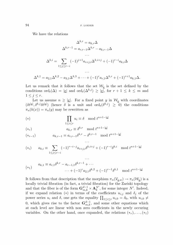
We have the relations
∆k,r = ak,r∆
∆k,r−1 = ar,r−1∆k,r − ak,r−1∆
. . .
∆k,i =∑
1≤j≤r−i
(−1)j+1ai+j,i∆k,i+j + (−1)r−iak,i∆
. . .
∆k,1 = a2,1∆k,2 − a3,1∆
k,3 + · · · + (−1)rar,1∆k,r + (−1)r+1ak,1∆.
Let us remark that it follows that the set We is the set defined by theconditions ordt(∆) = |e| and ordt(∆
k,j) ≥ |e|, for r + 1 ≤ k ≤ m and1 ≤ j ≤ r.
Let us assume n ≥ |e|. For a fixed point y in We with coordinates(δt|e|, δk,jδt|e|) (hence δ is a unit and ordt(δ
k,j) ≥ 0) the conditionsπn(h(x)) = πn(y) may be rewritten as
∏
1≤i≤r
ui ≡ δ mod tn+1−|e|(∗)
ak,r ≡ δk,r mod tn+1−|e|(∗r)
ak,r−1 ≡ ar,r−1δk,r − δk,r−1 mod tn+1−|e|(∗r−1)
. . .
ak,i ≡∑
1≤j≤r−i
(−1)r−i−jai+j,iδk,i+j + (−1)r−iδk,i mod tn+1−|e|(∗i)
. . .
ak,1 ≡ ar,1δk,r − ar−1,1δ
k,r−1 + · · ·
· · · + (−1)ra2,1δk,2 + (−1)r−1δk,1 mod tn+1−|e|(∗1)
It follows from that description that the morphism πn(Ve,w) → πn(We) is alocally trivial fibration (in fact, a trivial fibration) for the Zariski topologyand that the fiber is of the form Gd−1
m,k ×AN ′
k , for some integer N ′. Indeed,if we expand relation (∗) in terms of the coefficients ui,j and δj of thepower series ui and δ, one gets the equality
∏1≤i≤r ui,0 = δ0, with ui,0 6=
0, which gives rise to the factor Gd−1m,k , and some other equations which
at each level are linear with non zero coefficients in the newly occuringvariables. On the other hand, once expanded, the relations (∗r), . . . , (∗1)

MOTIVIC ZETA FUNCTIONS AND CASTLING TRANSFORMATIONS 95
give a triangular system of linear equations in the power series coefficientsof the variables ai,j. This gives the result except for the exact value ofN ′ which can be obtained either by direct calculation or by computingdimπn(Ve,w) − dimπn(We).
For arbitrary w, the situation reduces to the former one, since, up torenumbering the rows, the situation is just the same except that some ai,j’swith i, j ≤ r are now required to be of valuation ≥ 1, which has the soleeffect of replacing Zid by Zw in the statement.
Lemma 5.5. Set Y0 := h(Z0) and, for k ≥ 0, Yk = tkY0.
(1) For every e in Nr, h(Ze) = Y|e|.(2) Assume n ≥ k ≥ 0. For every constructible subset A of πn(Yk),
consider the preimage [h−1(A)] of A in πn(Z). The relation
[h−1(A)] = [A][SLr]Ln(r2−1)+k((m−r)r+1)
∑
|e|=k
∏
1≤i≤r
L−(m+1−i)ei
holds in Mk. Furthermore, if A is constructible with µ-action, the
same relation still holds in Mµk .
Proof. Assertion (1) follows from the fact, noted in the proof of Lem-ma 5.4, that the set We depends only on |e|. Let us denote it by W|e|.
To prove (2), we may assume A is contained in πn(Wk). Since thepreimage of πn(Wk) in πn(Z) is the disjoint union of the sets πn(Ve,w) with|e| = k and w in W , we have
[h−1(A)] =∑
|e|=k
[h−1(A) ∩ πn(Ve,w)].
One the other hand, by Lemma 5.4, we have
[h−1(A) ∩ πn(Ve,w)] = [Zw] × Ln(r2−1)+|e|((m−r)r+1)−P
1≤i≤r(m+1−i)ei ,
hence the result follows now from the relation
∑
w∈W
[Zw] = Lr2−1∏
2≤i≤r
(1 − L−i) = [SLr].
96 F. LOESER
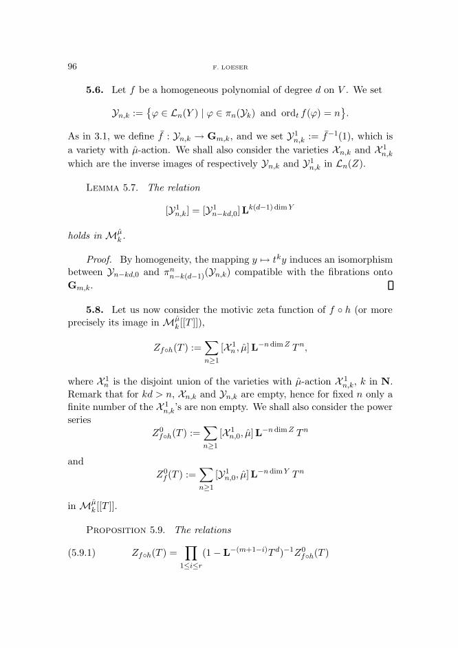
5.6. Let f be a homogeneous polynomial of degree d on V . We set
Yn,k :={ϕ ∈ Ln(Y ) | ϕ ∈ πn(Yk) and ordt f(ϕ) = n
}.
As in 3.1, we define f : Yn,k → Gm,k, and we set Y1n,k := f−1(1), which is
a variety with µ-action. We shall also consider the varieties Xn,k and X 1n,k
which are the inverse images of respectively Yn,k and Y1n,k in Ln(Z).
Lemma 5.7. The relation
[Y1n,k] = [Y1
n−kd,0]Lk(d−1) dimY
holds in Mµk .
Proof. By homogeneity, the mapping y 7→ tky induces an isomorphismbetween Yn−kd,0 and πn
n−k(d−1)(Yn,k) compatible with the fibrations onto
Gm,k.
5.8. Let us now consider the motivic zeta function of f ◦ h (or more
precisely its image in Mµk [[T ]]),
Zf◦h(T ) :=∑
n≥1
[X 1n , µ]L−n dimZ T n,
where X 1n is the disjoint union of the varieties with µ-action X 1
n,k, k in N.
Remark that for kd > n, Xn,k and Yn,k are empty, hence for fixed n only a
finite number of the X 1n,k’s are non empty. We shall also consider the power
series
Z0f◦h(T ) :=
∑
n≥1
[X 1n,0, µ]L−n dimZ T n
and
Z0f (T ) :=
∑
n≥1
[Y1n,0, µ]L−n dimY T n
in Mµk [[T ]].
Proposition 5.9. The relations
(5.9.1) Zf◦h(T ) =∏
1≤i≤r
(1 − L−(m+1−i)T d)−1Z0f◦h(T )

MOTIVIC ZETA FUNCTIONS AND CASTLING TRANSFORMATIONS 97
and
(5.9.2) Zf◦h(T ) = [SLr]∏
1≤i≤r
(1 − L−(m+1−i)T d)−1Z0f (T )
hold in Mµk [[T ]].
Proof. Since, as follows from Lemma 5.5,
Z0f◦h(T ) = [SLr]Z
0f (T ),
it is enough to prove (5.9.2). By Lemma 5.5, we have
[X 1n,k]L
−n dimZ = [SLr][Y1n,k]L
−n dimY Lk dimY∑
|e|=k
∏
1≤i≤r
L−(m+1−i)ei .
It follows from Lemma 5.7 that we may rewrite the last equality as
[X 1n,k]L
−n dimZ = [SLr][Y1n−kd,0]L
−(n−kd) dimY∑
|e|=k
∏
1≤i≤r
L−(m+1−i)ei ,
and we get the result by summing up the series.
5.10. Now we can conclude the proof of Theorem 4.2. Relation (4.2.1)
follows from writing (5.9.2) for both X1 and X2, and (4.2.2) follows from
(4.2.1) together with Lemma 3.2.
§6. Applications to the Milnor fibre and the Hodge spectrum
6.1. Monodromy
In this subsection 6.1 we assume that k = C. Let x be a point of X0 =
f−1(0). We fix a smooth metric on X. We set X×ε,η := B(x, ε) ∩ f−1(D×
η ),
with B(x, ε) the open ball of radius ε centered at x and D×η := Dη \ {0},
with Dη the open disk of radius η centered at 0. For 0 < η � ε � 1,
the restriction of f to X×ε,η is a locally trivial fibration, called the Milnor
fibration, onto D×η with fiber Fx, the Milnor fiber at x. The action of a
characteristic homeomorphism of this fibration on cohomology gives rise to
the monodromy operator
Mx : H ·(Fx,Q) −→ H ·(Fx,Q).
98 F. LOESER
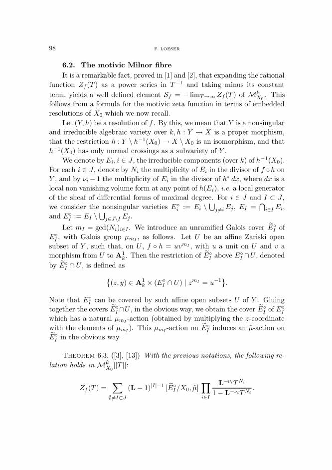
6.2. The motivic Milnor fibre
It is a remarkable fact, proved in [1] and [2], that expanding the rational
function Zf (T ) as a power series in T−1 and taking minus its constant
term, yields a well defined element Sf = − limT→∞ Zf (T ) of MµX0
. This
follows from a formula for the motivic zeta function in terms of embedded
resolutions of X0 which we now recall.
Let (Y, h) be a resolution of f . By this, we mean that Y is a nonsingular
and irreducible algebraic variety over k, h : Y → X is a proper morphism,
that the restriction h : Y \ h−1(X0) → X \ X0 is an isomorphism, and that
h−1(X0) has only normal crossings as a subvariety of Y .
We denote by Ei, i ∈ J , the irreducible components (over k) of h−1(X0).
For each i ∈ J , denote by Ni the multiplicity of Ei in the divisor of f ◦h on
Y , and by νi − 1 the multiplicity of Ei in the divisor of h∗ dx, where dx is a
local non vanishing volume form at any point of h(Ei), i.e. a local generator
of the sheaf of differential forms of maximal degree. For i ∈ J and I ⊂ J ,
we consider the nonsingular varieties E◦i := Ei \
⋃j 6=i Ej , EI =
⋂i∈I Ei,
and E◦I := EI \
⋃j∈J\I Ej.
Let mI = gcd(Ni)i∈I . We introduce an unramified Galois cover E◦I of
E◦I , with Galois group µmI
, as follows. Let U be an affine Zariski open
subset of Y , such that, on U , f ◦ h = uvmI , with u a unit on U and v a
morphism from U to A1k. Then the restriction of E◦
I above E◦I ∩U , denoted
by E◦I ∩ U , is defined as
{(z, y) ∈ A1
k × (E◦I ∩ U) | zmI = u−1
}.
Note that E◦I can be covered by such affine open subsets U of Y . Gluing
together the covers E◦I ∩U , in the obvious way, we obtain the cover E◦
I of E◦I
which has a natural µmI-action (obtained by multiplying the z-coordinate
with the elements of µmI). This µmI
-action on E◦I induces an µ-action on
E◦I in the obvious way.
Theorem 6.3. ([3], [13]) With the previous notations, the following re-
lation holds in MµX0
[[T ]]:
Zf (T ) =∑
∅6=I⊂J
(L− 1)|I|−1 [E◦I /X0, µ]
∏
i∈I
L−νiTNi
1 − L−νiTNi.
MOTIVIC ZETA FUNCTIONS AND CASTLING TRANSFORMATIONS 99
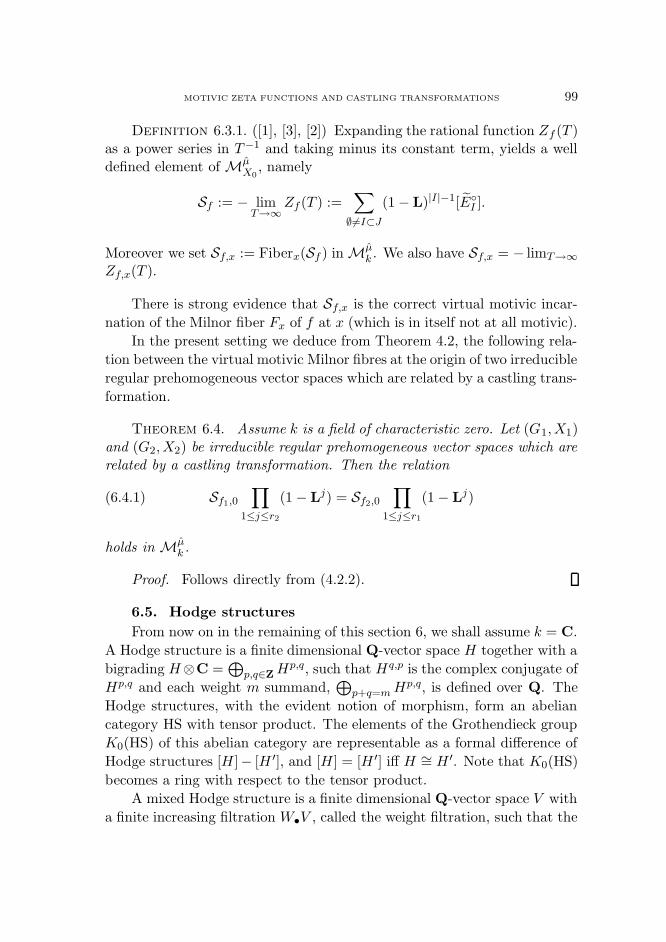
Definition 6.3.1. ([1], [3], [2]) Expanding the rational function Zf (T )as a power series in T−1 and taking minus its constant term, yields a welldefined element of Mµ
X0, namely
Sf := − limT→∞
Zf (T ) :=∑
∅6=I⊂J
(1 − L)|I|−1[E◦I ].
Moreover we set Sf,x := Fiberx(Sf ) in Mµk . We also have Sf,x = − limT→∞
Zf,x(T ).
There is strong evidence that Sf,x is the correct virtual motivic incar-
nation of the Milnor fiber Fx of f at x (which is in itself not at all motivic).
In the present setting we deduce from Theorem 4.2, the following rela-
tion between the virtual motivic Milnor fibres at the origin of two irreducible
regular prehomogeneous vector spaces which are related by a castling trans-
formation.
Theorem 6.4. Assume k is a field of characteristic zero. Let (G1, X1)and (G2, X2) be irreducible regular prehomogeneous vector spaces which are
related by a castling transformation. Then the relation
(6.4.1) Sf1,0
∏
1≤j≤r2
(1 − Lj) = Sf2,0
∏
1≤j≤r1
(1 − Lj)
holds in Mµk .
Proof. Follows directly from (4.2.2).
6.5. Hodge structures
From now on in the remaining of this section 6, we shall assume k = C.
A Hodge structure is a finite dimensional Q-vector space H together with a
bigrading H⊗C =⊕
p,q∈Z Hp,q, such that Hq,p is the complex conjugate of
Hp,q and each weight m summand,⊕
p+q=m Hp,q, is defined over Q. The
Hodge structures, with the evident notion of morphism, form an abelian
category HS with tensor product. The elements of the Grothendieck group
K0(HS) of this abelian category are representable as a formal difference of
Hodge structures [H]− [H ′], and [H] = [H ′] iff H ∼= H ′. Note that K0(HS)
becomes a ring with respect to the tensor product.
A mixed Hodge structure is a finite dimensional Q-vector space V with
a finite increasing filtration W•V , called the weight filtration, such that the
100 F. LOESER
associated graded vector space GrW• (V ) underlies a Hodge structure having
GrWm (V ) as weight m summand. Note that V determines in a natural way
an element [V ] in K0(HS), namely [V ] :=∑
m[GrWm (V )].
When X is an algebraic variety over k = C, the simplicial cohomology
groups H ic(X,Q) of X, with compact support, underly a natural mixed
Hodge structure, and the Hodge characteristic χh(X) of X (with compact
support) is defined by
χh(X) :=∑
i
(−1)i[Hic(X,Q)] ∈ K0(HS).
This yields a map χh : VarC → K0(HS) which factors through MC, be-
cause χh(A1k) is actually invertible in the ring K0(HS). When X is proper
and smooth, the mixed Hodge structure on H ic(X,Q) is in fact a Hodge
structure, the weight filtration being concentrated in weight i.
6.6. The Hodge spectrum
The cohomology groups H i(Fx,Q) of the Milnor fiber Fx carry a nat-
ural mixed Hodge structure ([20], [22], [15], [16]), which is compatible with
the semi-simplification of the monodromy operator Mx. Hence we can de-
fine the Hodge characteristic χh(Fx) of Fx by
χh(Fx) :=∑
i
(−1)i[Hi(Fx,Q)] ∈ K0(HS).
Actually by taking into account the monodromy action we can consider
χh(Fx) as an element of the Grothendieck group K0(HSmon) of the abelian
category HSmon of Hodge structures with an endomorphism of finite order.
Again K0(HSmon) is a ring by the tensor product.
There is a natural linear map, called the Hodge spectrum
hsp : K0(HSmon) −→ Z[t1/Z] :=⋃
n≥1
Z[t1/n, t−1/n],
with hsp([H]) :=∑
α∈Q∩[0,1[ tα(∑
p,q∈Z dim(Hp,q)α)tp, for any Hodge struc-
ture H with an endomorphism of finite order, where H p,qα is the generalized
eigenspace of Hp,q with respect to the eigenvalue e2π√−1α.
Let us denote by r the dimension of X. We recall that hsp(f, x) :=
(−1)r−1hsp(χh(Fx) − 1) is called the Hodge spectrum of f at x.
We denote by χh the canonical ring homomorphism (called the Hodge
characteristic)
χh : MµC −→ K0(HSmon),
MOTIVIC ZETA FUNCTIONS AND CASTLING TRANSFORMATIONS 101
which associates to any complex algebraic variety Z, with a good µn-action,
its Hodge characteristic together with the endomorphism induced by Z →
Z : z 7→ e2π√−1/nz.
Theorem 6.7. ([1]) Assume the above notation with k = C. Then we
have the following equality in K0(HSmon):
χh(Fx) = χh(Sf,x).
In particular it follows that
hsp(f, x) := (−1)r−1hsp(χh(Sf,x) − 1),
thus the motivic zeta function Zf,x(T ) completely determines the Hodge
spectrum of f at x.
Hence we deduce from Theorem 6.4, since hsp(χh(L)) = t, the follow-
ing:
Corollary 6.8. Assume k = C. Let (G1, X1) and (G2, X2) be irre-
ducible regular prehomogeneous vector spaces which are related by a castling
transformation. Then the following relation holds between the Hodge spectra
of f1 and f2 at 0
1 + (−1)mr1−1hsp(f1, 0)∏1≤j≤r1
(1 − tj)=
1 + (−1)mr2−1hsp(f2, 0)∏1≤j≤r2
(1 − tj).
§7. Some generalizations
7.1. Assume k is a field of characteristic zero. We now consider the
general case of prehomogeneous vector spaces which are not necessarily
irreducible and regular. In this setting we are given a connected linear
algebraic group G together with a linear action ρ : G → EndX on a finite
dimensional (linear) affine space X over k, such that the action is transitive
on a dense open set O = X \ S. Let Sj, 1 ≤ j ≤ `, be the k-irreducible
components of the singular set S which are of codimension 1 in X and
choose for every j a defining equation fj = 0 of Sj. Recall that a non-zero
k-rational function on X is a k-relative invariant of the G-action on X, if
there exists a k-rational character ν of G such that
f(ρ(g)x) = ν(g)f(x)
102 F. LOESER
for every g in G and x in X. The functions fj are k-relative invariants and
furthermore they are a basis of k-relative invariants in the sense that any
k-relative invariant of (G, ρ) is of the form cf µ1
1 · · · fµ`
` with c in k× and µj
in Z.
7.2. Motivic zeta function for several functions
Let X be a smooth k-variety of dimension r and consider ` functions
fj : X → A1k. We set X0 :=
⋂1≤j≤` (fj = 0).
For every n = (n1, . . . , n`) in (N×)`, we set |n| :=∑
1≤j≤` nj and define
Xn :={x ∈ L|n|(X) | ordt fj = nj, 1 ≤ j ≤ `
}.
Similarly as in 3.1, we have a natural morphism f : Xn → G`m,k, which
makes Xn a X0 × G`m,k-variety, for n in (N×)`. The motivic zeta function
attached to f = (f1, . . . , f`) is the formal series
Zf (T ) :=∑
n∈(N×)`
[Xn/X0 ×G`m,k]L
−|n|rT n
in MX0×G`m,k
[[T1, . . . , T`]]. It is a rational function of T = (T1, . . . , T`) (cf.
[1], [13], [2]). When ` = 1, the relation with the definition in 3.1 is the
following: the zeta function we just defined is the image of the former one
by the canonical morphism MµX0
→ MX0×Gm,kwhich to the class of a X0-
variety Y with µ-action assigns the class of Y ×µ Gm,k in MX0×Gm,k. For
x a point in X0(k), one defines similarly as in the ` = 1 case, Zf,x(T ) in
MG`m,k
[[T1, . . . , T`]].
7.3. As in 4.1 we consider a connected linear algebraic group G over
k and ρ be a representation of G in Amk . Write m = r1 + r2 and define Xj ,
Gj and ρj , j = 1, 2 as in 4.1. We assume they give rise to prehomogeneous
vector spaces for j = 1, 2, and we say that the prehomogeneous vector
spaces (G1, X1) and (G2, X2) are related by a castling transformation. We
choose a basis of k-relative invariants f1 = (f1,i), 1 ≤ j ≤ `1 and f2 = (f1,2),
1 ≤ j ≤ `2, respectively. As in 4.1, we consider the quotient spaces Xi/SLri
as embedded by the Plucker embedding the same affine space V , and up
to renumbering the f1,i’s and multiplying them by non-zero constants, one
may assume that both the f1,i’s and the f2,i’s are the pullback of the same
homogeneous polynomials fi of degree di in V , cf. [17], [6]. In particular,
we may write `1 = `2 = `. We set d = (di) in (N×)`.
We have the following generalization of Theorem 4.2.

MOTIVIC ZETA FUNCTIONS AND CASTLING TRANSFORMATIONS 103
Theorem 7.4. Let (G1, X1) and (G2, X2) be prehomogeneous vector
spaces related by a castling transformation. Then the relations
(7.4.1)
Zf1(T )[SLr2,k]
∏
1≤j≤r1
(1 − T dL−j) = Zf2(T )[SLr1,k]
∏
1≤j≤r2
(1 − T dL−j)
and
(7.4.2) Zf1,0(T )∏
1≤j≤r1
(T−d − L−j)∏
1≤j≤r2
(1 − L−j) =
Zf2,0(T )∏
1≤j≤r2
(T−d − L−j)∏
1≤j≤r1
(1 − L−j)
hold in MG`m,k
[[T ]], with T = (T1, . . . , T`) and [SLr] = Lr2−1∏
2≤i≤r(1 −
L−i).
Proof. The proof is just the same as the proof of Theorem 4.2.
Remark 7.5. There is an obvious generalization of Theorem 7.4 toparabolic castling transforms as introduced in [19], cf. [6]. Details are leftto the reader.
7.6. Similarly as for the case of one function in 6.3.1, Guibert proves
in [5] that, for every α in (N×)`, − limT→∞ Zf (T α) is a well defined element
of MX0×G`m,C
, independent of α. Let us denote it by Sf and set Sf,x :=
Fiberx(Sf ). We also have Sf,x = − limT→∞ Zf,x(T α), for every α in (N×)`.
Remark 7.7. When k = C, G. Guibert shows in [5] how Sabbah’sAlexander invariants of f (cf. [14]) may be recovered from the motivic zetafunction Zf .
Remark 7.8. It would be interesting to investigate what information iscontained in the Hodge realization of Sf . It is quite likely that there shouldbe some connections with recent work of A. Libgober in [12].
The following statement follows directly from Theorem 7.4.
Theorem 7.9. Let (G1, X1) and (G2, X2) be prehomogeneous vector
spaces related by a castling transformation. Then the relation
(7.9.1) Sf1,0
∏
1≤j≤r2
(1 − Lj) = Sf2,0
∏
1≤j≤r1
(1 − Lj)
holds in MX0×G`m,C
.
104 F. LOESER
References
[1] J. Denef and F. Loeser, Motivic Igusa zeta functions, J. Algebraic Geom., 7 (1998),
505–537.
[2] J. Denef and F. Loeser, Geometry on arc spaces of algebraic varieties, Proceedings of
3rd European Congress of Mathematics, Barcelona 2000, Progress in Mathematics
201, Birkhauser (2001), pp. 327–348.
[3] J. Denef and F. Loeser, Lefschetz numbers of iterates of the monodromy and truncated
arcs, Topology, 41 (2002), 1031–1040.
[4] J. Gordon, Motivic Haar measure on reductive groups, preprint, March 2002, avail-
able at math.AG/0203106.
[5] G. Guibert, Fonction zeta motivique associee a une famille de series de deux vari-
ables, C. R. Acad. Sci. Paris Ser. I Math., 333 (2001), 457–460.
[6] H. Hosokawa, Igusa local zeta functions and parabolic castling transformation of
prehomogeneous vector spaces, J. Number Theory, 74 (1999), 148–171.
[7] J. Igusa, On functional equations of complex powers, Invent. Math., 85 (1986), 1–29.
[8] J. Igusa, On the arithmetic of a singular invariant, Amer. J. Math., 110 (1988),
197–233.
[9] J. Igusa, b-functions and p-adic integrals, Algebraic analysis, Vol. I, Academic Press,
Boston, MA, 1988, pp. 231–241.
[10] J. Igusa, Local zeta functions of certain prehomogeneous vector spaces, Amer. J.
Math., 114 (1992), 251–296.
[11] T. Kimura, The b-functions and holonomy diagrams of irreducible regular prehomo-
geneous vector spaces, Nagoya Math. J., 85 (1982), 1–80.
[12] A. Libgober, Hodge decomposition of Alexander invariants, preprint, October 2001,
available at math.AG/0108018.
[13] E. Looijenga, Motivic Measures, Asterisque 276, Seminaire Bourbaki, expose 874
(2002), 267–297.
[14] C. Sabbah, Modules d’Alexander et D-modules, Duke Math. J., 60 (1990), 729–814.
[15] M. Saito, Modules de Hodge polarisables, Publ. Res. Inst. Math. Sci., 24 (1988),
849–995.
[16] M. Saito, Mixed Hodge modules, Publ. Res. Inst. Math. Sci., 26 (1990), 221–333.
[17] M. Sato and T. Kimura, A classification of irreducible prehomogeneous vector spaces
and their relative invariants, Nagoya Math. J., 65 (1977), 1–155.
[18] M. Sato and T. Shintani, On zeta functions associated with prehomogeneous vector
spaces, Ann. of Math., 100 (1974), 131–170.
[19] Y. Teranishi, Relative invariants and b-functions of prehomogeneous vector spaces
(G × GL(d1, . . . , dr), p1, M(n, C)), Nagoya Math. J., 98 (1985), 139–156.
[20] J. Steenbrink, Mixed Hodge structures on the vanishing cohomology, Real and Com-
plex Singularities, Sijthoff and Noordhoff, Alphen aan den Rijn (1977), 525–563.
[21] J. Steenbrink, The spectrum of hypersurface singularities, Theorie de Hodge, Luminy
1987, Asterisque, 179-180 (1989), 163–184.
[22] A. Varchenko, Asymptotic Hodge structure in the vanishing cohomology, Math. USSR
Izvestija, 18 (1982), 469–512.
MOTIVIC ZETA FUNCTIONS AND CASTLING TRANSFORMATIONS 105
[23] T. Yano and I. Ozeki, The b-function of a prehomogeneous vector space
(SL(5)×GL(4), Λ2 ⊗Λ1). Microlocal structure of the regular prehomogeneous vector
space associated with SL(5)×GL(4). II, Research on prehomogeneous vector spaces
(Kyoto, 1996), RIMS Kokyuroku, 999 (1997), 92–115.
Ecole Normale Superieure
Departement de mathematiques et applications
45 rue d’Ulm
75230 Paris Cedex 05
France
(UMR 8553 du CNRS )[email protected]