motif comparisons and p-values - bioconductor

Motif comparisons and P-values

Benjamin Jean-Marie Tremblay∗

17 October 2021

AbstractTwo important but not often discussed topics with regards to motifs are motif comparisons and

P-values. These are explored here, including implementation details and example use cases.

Contents1 Introduction 1

2 Motif comparisons 12.1 An overview of available comparison metrics . . . . . . . . . . . . . . . . . . . . . . . . . . . . 22.2 Comparison parameters . . . . . . . . . . . . . . . . . . . . . . . . . . . . . . . . . . . . . . . 32.3 Comparison P-values . . . . . . . . . . . . . . . . . . . . . . . . . . . . . . . . . . . . . . . . . 6

3 Motif trees with ggtree 63.1 Using motif_tree() . . . . . . . . . . . . . . . . . . . . . . . . . . . . . . . . . . . . . . . . . 63.2 Using compare_motifs() and ggtree() . . . . . . . . . . . . . . . . . . . . . . . . . . . . . . 73.3 Plotting motifs alongside trees . . . . . . . . . . . . . . . . . . . . . . . . . . . . . . . . . . . 9

4 Motif P-values 104.1 The dynamic programming algorithm for calculating P-values and scores . . . . . . . . . . . . 114.2 The branch-and-bound algorithm for calculating P-values from scores . . . . . . . . . . . . . 144.3 The random subsetting algorithm for calculating scores from P-values . . . . . . . . . . . . . 15

Session info 17

References 18

1 IntroductionThis vignette covers motif comparisons (including metrics, parameters and clustering) and P-values. For anintroduction to sequence motifs, see the introductory vignette. For a basic overview of available motif-relatedfunctions, see the motif manipulation vignette. For sequence-related utilities, see the sequences vignette.

2 Motif comparisonsThere a couple of functions available in other Bioconductor packages which allow for motif comparison,such as PWMSimlarity() (TFBSTools) and motifSimilarity() (PWMEnrich). Unfortunately these functionsare not designed for comparing large numbers of motifs. Furthermore they are restrictive in their optionrange. The universalmotif package aims to fix this by providing the compare_motifs() function. Several

∗[email protected]

1

mailto:[email protected]

other functions also make use of the core compare_motifs() functionality, including merge_motifs() andview_motifs().

2.1 An overview of available comparison metricsThis function has been written to allow comparisons using any of the following metrics:

• Euclidean distance (EUCL)• Weighted Euclidean distance (WEUCL)• Kullback-Leibler divergence (KL) (Kullback and Leibler 1951; Roepcke et al. 2005)• Hellinger distance (HELL) (Hellinger 1909)• Squared Euclidean distance (SEUCL)• Manhattan distance (MAN)• Pearson correlation coefficient (PCC)• Weighted Pearson correlation coefficient (WPCC)• Sandelin-Wasserman similarity (SW; or sum of squared distances) (Sandelin and Wasserman 2004)• Average log-likelihood ratio (ALLR) (Wang and Stormo 2003)• Lower limit average log-likelihood ratio (ALLR_LL; minimum column score of -2) (Mahony, Auron, and

Benos 2007)• Bhattacharyya coefficient (BHAT) (Bhattacharyya 1943)

For clarity, here are the R implementations of these metrics:EUCL <- function(c1, c2) {

sqrt( sum( (c1 - c2)^2 ) )}

WEUCL <- function(c1, c2, bkg1, bkg2) {sqrt( sum( (bkg1 + bkg2) * (c1 - c2)^2 ) )

}

KL <- function(c1, c2) {( sum(c1 * log(c1 / c2)) + sum(c2 * log(c2 / c1)) ) / 2

}

HELL <- function(c1, c2) {sqrt( sum( ( sqrt(c1) - sqrt(c2) )^2 ) ) / sqrt(2)

}

SEUCL <- function(c1, c2) {sum( (c1 - c2)^2 )

}

MAN <- function(c1, c2) {sum ( abs(c1 - c2) )

}

PCC <- function(c1, c2) {n <- length(c1)top <- n * sum(c1 * c2) - sum(c1) * sum(c2)bot <- sqrt( ( n * sum(c1^2) - sum(c1)^2 ) * ( n * sum(c2^2) - sum(c2)^2 ) )top / bot

}

WPCC <- function(c1, c2, bkg1, bkg2) {

2

weights <- bkg1 + bkg2mean1 <- sum(weights * c1)mean2 <- sum(weights * c2)var1 <- sum(weights * (c1 - mean1)^2)var2 <- sum(weights * (c2 - mean2)^2)cov <- sum(weights * (c1 - mean1) * (c2 - mean2))cov / sqrt(var1 * var2)

}

SW <- function(c1, c2) {2 - sum( (c1 - c2)^2 )

}

ALLR <- function(c1, c2, bkg1, bkg2, nsites1, nsites2) {left <- sum( c2 * nsites2 * log(c1 / bkg1) )right <- sum( c1 * nsites1 * log(c2 / bkg2) )( left + right ) / ( nsites1 + nsites2 )

}

BHAT <- function(c1, c2) {sum( sqrt(c1 * c2) )

}

Motif comparison involves comparing a single column from each motif individually, and adding up the scoresfrom all column comparisons. Since this causes the score to be highly dependent on motif length, the scorescan instead be averaged using the arithmetic mean, geometric mean, median, or Fisher Z-transform.

If you’re curious as to how the comparison metrics perform, two columns can be compared individually usingcompare_columns():c1 <- c(0.7, 0.1, 0.1, 0.1)c2 <- c(0.5, 0.0, 0.2, 0.3)

compare_columns(c1, c2, "PCC")#> [1] 0.8006408compare_columns(c1, c2, "EUCL")#> [1] 0.3162278

Note that some metrics do not work with zero values, and small pseudocounts are automatically added tomotifs for the following:

• KL• ALLR• ALLR_LL

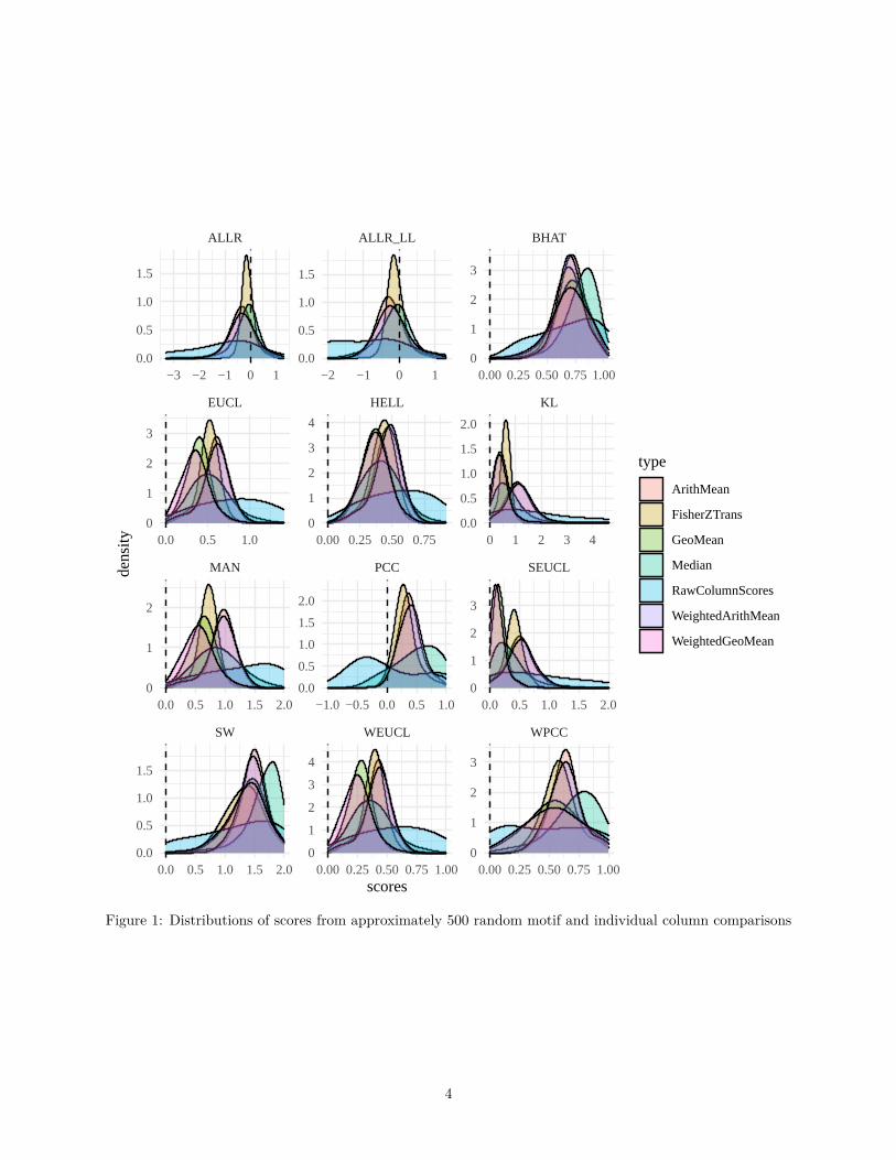
As seen in figure 1, the distributions for random individual column comparisons tend to be very skewed. Thisis usually remedied when comparing the entire motif, though some metrics still perform poorly in this regard.

#> `summarise()` has grouped output by 'key'. You can override using the `.groups`#> argument.

2.2 Comparison parametersThere are several key parameters to keep in mind when comparing motifs. Some of these are:

• method: one of the metrics listed previously• tryRC: choose whether to try comparing the reverse complements of each motif as well

3

SW WEUCL WPCC

MAN PCC SEUCL

EUCL HELL KL

ALLR ALLR_LL BHAT

0.0 0.5 1.0 1.5 2.0 0.00 0.25 0.50 0.75 1.00 0.00 0.25 0.50 0.75 1.00

0.0 0.5 1.0 1.5 2.0 −1.0 −0.5 0.0 0.5 1.0 0.0 0.5 1.0 1.5 2.0

0.0 0.5 1.0 0.00 0.25 0.50 0.75 0 1 2 3 4

−3 −2 −1 0 1 −2 −1 0 1 0.00 0.25 0.50 0.75 1.000

1

2

3

0.0

0.5

1.0

1.5

2.0

0

1

2

3

0

1

2

3

0.0

0.5

1.0

1.5

0

1

2

3

4

0.0

0.5

1.0

1.5

2.0

0

1

2

3

4

0.0

0.5

1.0

1.5

0

1

2

3

0

1

2

0.0

0.5

1.0

1.5

scores

dens

ity

type

ArithMean

FisherZTrans

GeoMean

Median

RawColumnScores

WeightedArithMean

WeightedGeoMean

Figure 1: Distributions of scores from approximately 500 random motif and individual column comparisons

4

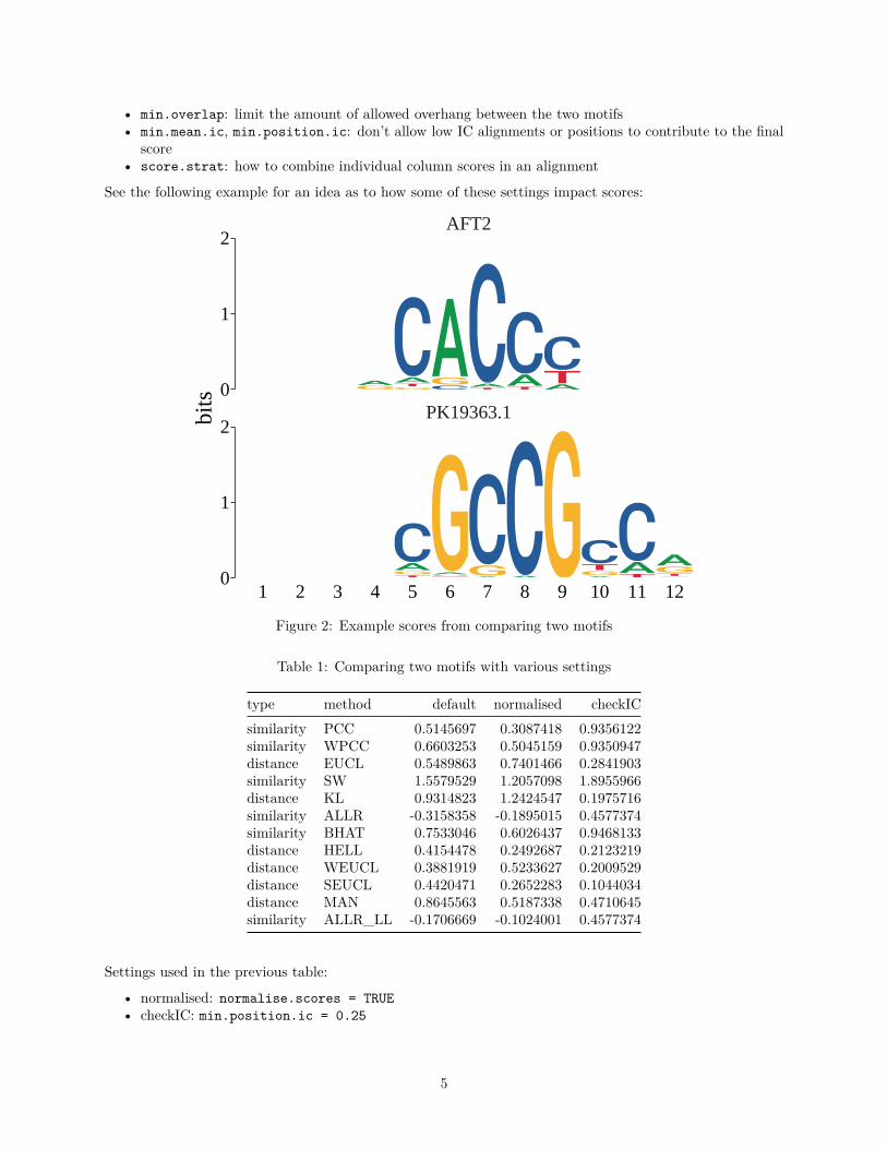
• min.overlap: limit the amount of allowed overhang between the two motifs• min.mean.ic, min.position.ic: don’t allow low IC alignments or positions to contribute to the final

score• score.strat: how to combine individual column scores in an alignment

See the following example for an idea as to how some of these settings impact scores:

PK19363.1

AFT2

1 2 3 4 5 6 7 8 9 10 11 12

0

1

2

0

1

2bits

Figure 2: Example scores from comparing two motifs

Table 1: Comparing two motifs with various settings

type method default normalised checkICsimilarity PCC 0.5145697 0.3087418 0.9356122similarity WPCC 0.6603253 0.5045159 0.9350947distance EUCL 0.5489863 0.7401466 0.2841903similarity SW 1.5579529 1.2057098 1.8955966distance KL 0.9314823 1.2424547 0.1975716similarity ALLR -0.3158358 -0.1895015 0.4577374similarity BHAT 0.7533046 0.6026437 0.9468133distance HELL 0.4154478 0.2492687 0.2123219distance WEUCL 0.3881919 0.5233627 0.2009529distance SEUCL 0.4420471 0.2652283 0.1044034distance MAN 0.8645563 0.5187338 0.4710645similarity ALLR_LL -0.1706669 -0.1024001 0.4577374

Settings used in the previous table:

• normalised: normalise.scores = TRUE• checkIC: min.position.ic = 0.25

5

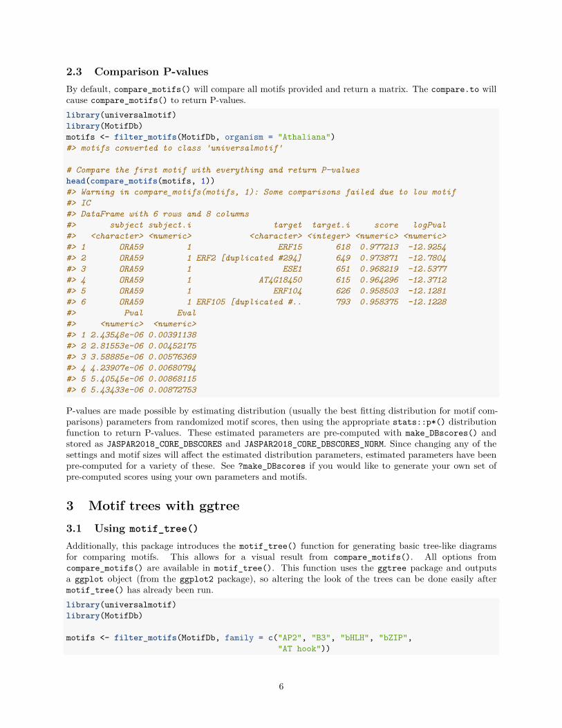
2.3 Comparison P-valuesBy default, compare_motifs() will compare all motifs provided and return a matrix. The compare.to willcause compare_motifs() to return P-values.library(universalmotif)library(MotifDb)motifs <- filter_motifs(MotifDb, organism = "Athaliana")#> motifs converted to class 'universalmotif'

# Compare the first motif with everything and return P-valueshead(compare_motifs(motifs, 1))#> Warning in compare_motifs(motifs, 1): Some comparisons failed due to low motif#> IC#> DataFrame with 6 rows and 8 columns#> subject subject.i target target.i score logPval#> <character> <numeric> <character> <integer> <numeric> <numeric>#> 1 ORA59 1 ERF15 618 0.977213 -12.9254#> 2 ORA59 1 ERF2 [duplicated #294] 649 0.973871 -12.7804#> 3 ORA59 1 ESE1 651 0.968219 -12.5377#> 4 ORA59 1 AT4G18450 615 0.964296 -12.3712#> 5 ORA59 1 ERF104 626 0.958503 -12.1281#> 6 ORA59 1 ERF105 [duplicated #.. 793 0.958375 -12.1228#> Pval Eval#> <numeric> <numeric>#> 1 2.43548e-06 0.00391138#> 2 2.81553e-06 0.00452175#> 3 3.58885e-06 0.00576369#> 4 4.23907e-06 0.00680794#> 5 5.40545e-06 0.00868115#> 6 5.43433e-06 0.00872753

P-values are made possible by estimating distribution (usually the best fitting distribution for motif com-parisons) parameters from randomized motif scores, then using the appropriate stats::p*() distributionfunction to return P-values. These estimated parameters are pre-computed with make_DBscores() andstored as JASPAR2018_CORE_DBSCORES and JASPAR2018_CORE_DBSCORES_NORM. Since changing any of thesettings and motif sizes will affect the estimated distribution parameters, estimated parameters have beenpre-computed for a variety of these. See ?make_DBscores if you would like to generate your own set ofpre-computed scores using your own parameters and motifs.

3 Motif trees with ggtree3.1 Using motif_tree()

Additionally, this package introduces the motif_tree() function for generating basic tree-like diagramsfor comparing motifs. This allows for a visual result from compare_motifs(). All options fromcompare_motifs() are available in motif_tree(). This function uses the ggtree package and outputsa ggplot object (from the ggplot2 package), so altering the look of the trees can be done easily aftermotif_tree() has already been run.library(universalmotif)library(MotifDb)

motifs <- filter_motifs(MotifDb, family = c("AP2", "B3", "bHLH", "bZIP","AT hook"))

6

#> motifs converted to class 'universalmotif'motifs <- motifs[sample(seq_along(motifs), 100)]tree <- motif_tree(motifs, layout = "daylight", linecol = "family")#> Average angle change [1] 0.0864633075463251#> Average angle change [2] 0.0210093959224575

## Make some changes to the tree in regular ggplot2 fashion:# tree <- tree + ...

tree

0

AP2

AT hook

B3

bHLH

bZIP

3.2 Using compare_motifs() and ggtree()

While motif_tree() works as a quick and convenient tree-building function, it can be inconvenient whenmore control is required over tree construction. For this purpose, the following code goes through how exactlymotif_tree() generates trees.library(universalmotif)library(MotifDb)library(ggtree)library(ggplot2)

motifs <- convert_motifs(MotifDb)motifs <- filter_motifs(motifs, organism = "Athaliana")motifs <- motifs[sample(seq_along(motifs), 25)]

## Step 1: compare motifs

comparisons <- compare_motifs(motifs, method = "PCC", min.mean.ic = 0,score.strat = "a.mean")

7

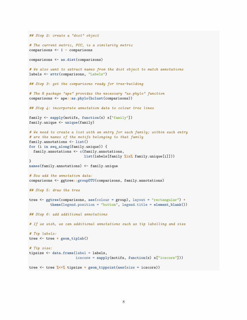
## Step 2: create a "dist" object

# The current metric, PCC, is a similarity metriccomparisons <- 1 - comparisons

comparisons <- as.dist(comparisons)

# We also want to extract names from the dist object to match annotationslabels <- attr(comparisons, "Labels")

## Step 3: get the comparisons ready for tree-building

# The R package "ape" provides the necessary "as.phylo" functioncomparisons <- ape::as.phylo(hclust(comparisons))

## Step 4: incorporate annotation data to colour tree lines

family <- sapply(motifs, function(x) x["family"])family.unique <- unique(family)

# We need to create a list with an entry for each family; within each entry# are the names of the motifs belonging to that familyfamily.annotations <- list()for (i in seq_along(family.unique)) {

family.annotations <- c(family.annotations,list(labels[family %in% family.unique[i]]))

}names(family.annotations) <- family.unique

# Now add the annotation data:comparisons <- ggtree::groupOTU(comparisons, family.annotations)

## Step 5: draw the tree

tree <- ggtree(comparisons, aes(colour = group), layout = "rectangular") +theme(legend.position = "bottom", legend.title = element_blank())

## Step 6: add additional annotations

# If we wish, we can additional annotations such as tip labelling and size

# Tip labels:tree <- tree + geom_tiplab()

# Tip size:tipsize <- data.frame(label = labels,

icscore = sapply(motifs, function(x) x["icscore"]))

tree <- tree %<+% tipsize + geom_tippoint(aes(size = icscore))

8

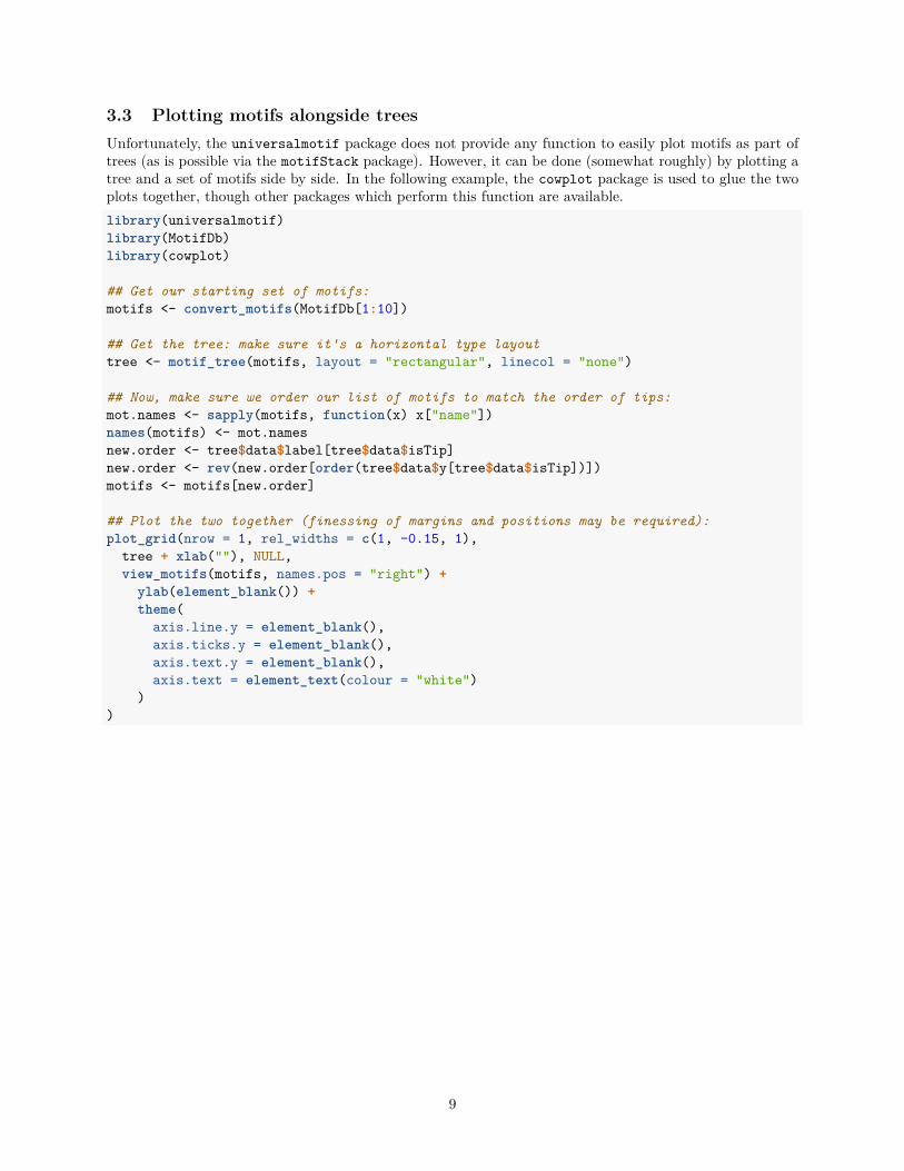
3.3 Plotting motifs alongside treesUnfortunately, the universalmotif package does not provide any function to easily plot motifs as part oftrees (as is possible via the motifStack package). However, it can be done (somewhat roughly) by plotting atree and a set of motifs side by side. In the following example, the cowplot package is used to glue the twoplots together, though other packages which perform this function are available.library(universalmotif)library(MotifDb)library(cowplot)

## Get our starting set of motifs:motifs <- convert_motifs(MotifDb[1:10])

## Get the tree: make sure it's a horizontal type layouttree <- motif_tree(motifs, layout = "rectangular", linecol = "none")

## Now, make sure we order our list of motifs to match the order of tips:mot.names <- sapply(motifs, function(x) x["name"])names(motifs) <- mot.namesnew.order <- tree$data$label[tree$data$isTip]new.order <- rev(new.order[order(tree$data$y[tree$data$isTip])])motifs <- motifs[new.order]

## Plot the two together (finessing of margins and positions may be required):plot_grid(nrow = 1, rel_widths = c(1, -0.15, 1),

tree + xlab(""), NULL,view_motifs(motifs, names.pos = "right") +

ylab(element_blank()) +theme(

axis.line.y = element_blank(),axis.ticks.y = element_blank(),axis.text.y = element_blank(),axis.text = element_text(colour = "white")

))

9

GZF3

FZF1 [RC]

ECM23 [RC]

CST6

FKH2 [RC]

EDS1

ABF2 [RC]

GSM1 [RC]

CAT8

GIS1 [RC]1 2 3 4 5 6 7

4 Motif P-valuesMotif P-values are not usually discussed outside of the bioinformatics literature, but are actually quite achallenging topic. To illustrate this, consider the following example motif:library(universalmotif)

m <- matrix(c(0.10,0.27,0.23,0.19,0.29,0.28,0.51,0.12,0.34,0.26,0.36,0.29,0.51,0.38,0.23,0.16,0.17,0.21,0.23,0.36,0.45,0.05,0.02,0.13,0.27,0.38,0.26,0.38,0.12,0.31,0.09,0.40,0.24,0.30,0.21,0.19,0.05,0.30,0.31,0.08),

byrow = TRUE, nrow = 4)motif <- create_motif(m, alphabet = "DNA", type = "PWM")motif#>#> Motif name: motif#> Alphabet: DNA#> Type: PWM#> Strands: +-#> Total IC: 10.03#> Pseudocount: 0#> Consensus: SHCNNNRNNV#>#> S H C N N N R N N V#> A -1.32 0.10 -0.12 -0.40 0.21 0.15 1.04 -1.07 0.44 0.04#> C 0.53 0.20 1.03 0.60 -0.12 -0.66 -0.54 -0.27 -0.12 0.51#> G 0.85 -2.34 -3.64 -0.94 0.11 0.59 0.07 0.59 -1.06 0.30

10

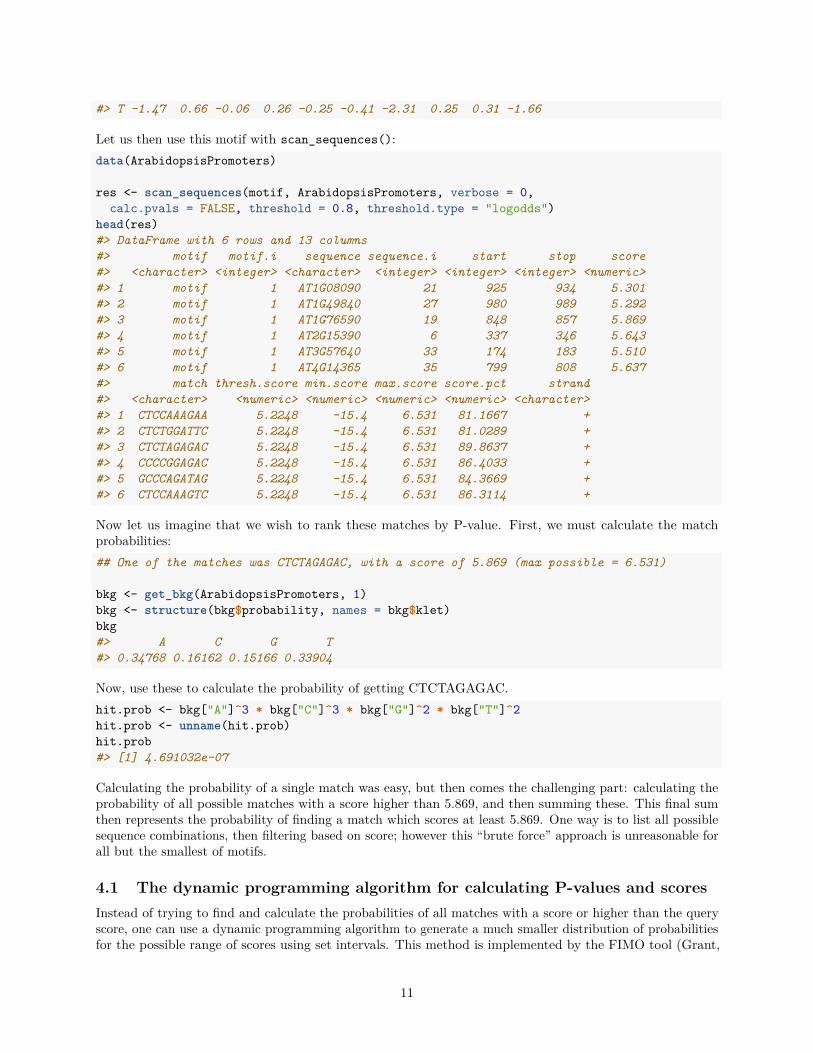
#> T -1.47 0.66 -0.06 0.26 -0.25 -0.41 -2.31 0.25 0.31 -1.66

Let us then use this motif with scan_sequences():data(ArabidopsisPromoters)

res <- scan_sequences(motif, ArabidopsisPromoters, verbose = 0,calc.pvals = FALSE, threshold = 0.8, threshold.type = "logodds")

head(res)#> DataFrame with 6 rows and 13 columns#> motif motif.i sequence sequence.i start stop score#> <character> <integer> <character> <integer> <integer> <integer> <numeric>#> 1 motif 1 AT1G08090 21 925 934 5.301#> 2 motif 1 AT1G49840 27 980 989 5.292#> 3 motif 1 AT1G76590 19 848 857 5.869#> 4 motif 1 AT2G15390 6 337 346 5.643#> 5 motif 1 AT3G57640 33 174 183 5.510#> 6 motif 1 AT4G14365 35 799 808 5.637#> match thresh.score min.score max.score score.pct strand#> <character> <numeric> <numeric> <numeric> <numeric> <character>#> 1 CTCCAAAGAA 5.2248 -15.4 6.531 81.1667 +#> 2 CTCTGGATTC 5.2248 -15.4 6.531 81.0289 +#> 3 CTCTAGAGAC 5.2248 -15.4 6.531 89.8637 +#> 4 CCCCGGAGAC 5.2248 -15.4 6.531 86.4033 +#> 5 GCCCAGATAG 5.2248 -15.4 6.531 84.3669 +#> 6 CTCCAAAGTC 5.2248 -15.4 6.531 86.3114 +

Now let us imagine that we wish to rank these matches by P-value. First, we must calculate the matchprobabilities:## One of the matches was CTCTAGAGAC, with a score of 5.869 (max possible = 6.531)

bkg <- get_bkg(ArabidopsisPromoters, 1)bkg <- structure(bkg$probability, names = bkg$klet)bkg#> A C G T#> 0.34768 0.16162 0.15166 0.33904

Now, use these to calculate the probability of getting CTCTAGAGAC.hit.prob <- bkg["A"]^3 * bkg["C"]^3 * bkg["G"]^2 * bkg["T"]^2hit.prob <- unname(hit.prob)hit.prob#> [1] 4.691032e-07

Calculating the probability of a single match was easy, but then comes the challenging part: calculating theprobability of all possible matches with a score higher than 5.869, and then summing these. This final sumthen represents the probability of finding a match which scores at least 5.869. One way is to list all possiblesequence combinations, then filtering based on score; however this “brute force” approach is unreasonable forall but the smallest of motifs.

4.1 The dynamic programming algorithm for calculating P-values and scoresInstead of trying to find and calculate the probabilities of all matches with a score or higher than the queryscore, one can use a dynamic programming algorithm to generate a much smaller distribution of probabilitiesfor the possible range of scores using set intervals. This method is implemented by the FIMO tool (Grant,

11

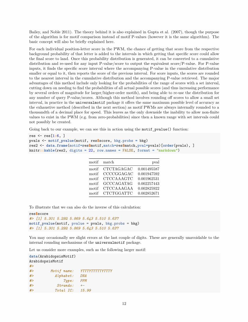
Bailey, and Noble 2011). The theory behind it is also explained in Gupta et al. (2007), though the purposeof the algorithm is for motif comparison instead of motif P-values (however it is the same algorithm). Thebasic concept will also be briefly explained here.

For each individual position-letter score in the PWM, the chance of getting that score from the respectivebackground probability of that letter is added to the intervals in which getting that specific score could allowthe final score to land. Once this probability distribution is generated, it can be converted to a cumulativedistribution and re-used for any input P-value/score to output the equivalent score/P-value. For P-valueinputs, it finds the specific score interval where the accompanying P-value in the cumulative distributionsmaller or equal to it, then reports the score of the previous interval. For score inputs, the scores are roundedto the nearest interval in the cumulative distribution and the accompanying P-value retrieved. The majoradvantages of this method include only looking for the probabilities of the range of scores with a set interval,cutting down on needing to find the probabilities of all actual possible scores (and thus increasing performanceby several orders of magnitude for larger/higher-order motifs), and being able to re-use the distribution forany number of query P-value/scores. Although this method involves rounding off scores to allow a small setinterval, in practice in the universalmotif package it offers the same maximum possible level of accuracy asthe exhaustive method (described in the next section) as motif PWMs are always internally rounded to athousandth of a decimal place for speed. This leaves as the only downside the inability to allow non-finitevalues to exist in the PWM (e.g. from zero-probabilities) since then a known range with set intervals couldnot possibly be created.

Going back to our example, we can see this in action using the motif_pvalue() function:res <- res[1:6, ]pvals <- motif_pvalue(motif, res$score, bkg.probs = bkg)res2 <- data.frame(motif=res$motif,match=res$match,pval=pvals)[order(pvals), ]knitr::kable(res2, digits = 22, row.names = FALSE, format = "markdown")

motif match pvalmotif CTCTAGAGAC 0.001495587motif CCCCGGAGAC 0.001947592motif CTCCAAAGTC 0.001962531motif GCCCAGATAG 0.002257443motif CTCCAAAGAA 0.002825922motif CTCTGGATTC 0.002852671

To illustrate that we can also do the inverse of this calculation:res$score#> [1] 5.301 5.292 5.869 5.643 5.510 5.637motif_pvalue(motif, pvalue = pvals, bkg.probs = bkg)#> [1] 5.301 5.292 5.869 5.643 5.510 5.637

You may occasionally see slight errors at the last couple of digits. These are generally unavoidable to theinternal rounding mechanisms of the universalmotif package.

Let us consider more examples, such as the following larger motif:data(ArabidopsisMotif)ArabidopsisMotif#>#> Motif name: YTTTYTTTTTYTTTY#> Alphabet: DNA#> Type: PPM#> Strands: +-#> Total IC: 15.99

12

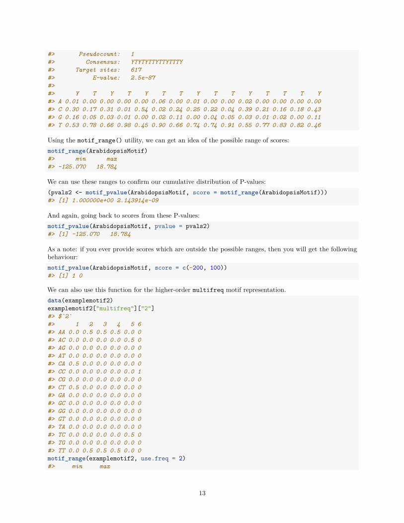
#> Pseudocount: 1#> Consensus: YTYTYTTYTTYTTTY#> Target sites: 617#> E-value: 2.5e-87#>#> Y T Y T Y T T Y T T Y T T T Y#> A 0.01 0.00 0.00 0.00 0.00 0.06 0.00 0.01 0.00 0.00 0.02 0.00 0.00 0.00 0.00#> C 0.30 0.17 0.31 0.01 0.54 0.02 0.24 0.25 0.22 0.04 0.39 0.21 0.16 0.18 0.43#> G 0.16 0.05 0.03 0.01 0.00 0.02 0.11 0.00 0.04 0.05 0.03 0.01 0.02 0.00 0.11#> T 0.53 0.78 0.66 0.98 0.45 0.90 0.66 0.74 0.74 0.91 0.55 0.77 0.83 0.82 0.46

Using the motif_range() utility, we can get an idea of the possible range of scores:motif_range(ArabidopsisMotif)#> min max#> -125.070 18.784

We can use these ranges to confirm our cumulative distribution of P-values:(pvals2 <- motif_pvalue(ArabidopsisMotif, score = motif_range(ArabidopsisMotif)))#> [1] 1.000000e+00 2.143914e-09

And again, going back to scores from these P-values:motif_pvalue(ArabidopsisMotif, pvalue = pvals2)#> [1] -125.070 18.784

As a note: if you ever provide scores which are outside the possible ranges, then you will get the followingbehaviour:motif_pvalue(ArabidopsisMotif, score = c(-200, 100))#> [1] 1 0

We can also use this function for the higher-order multifreq motif representation.data(examplemotif2)examplemotif2["multifreq"]["2"]#> $`2`#> 1 2 3 4 5 6#> AA 0.0 0.5 0.5 0.5 0.0 0#> AC 0.0 0.0 0.0 0.0 0.5 0#> AG 0.0 0.0 0.0 0.0 0.0 0#> AT 0.0 0.0 0.0 0.0 0.0 0#> CA 0.5 0.0 0.0 0.0 0.0 0#> CC 0.0 0.0 0.0 0.0 0.0 1#> CG 0.0 0.0 0.0 0.0 0.0 0#> CT 0.5 0.0 0.0 0.0 0.0 0#> GA 0.0 0.0 0.0 0.0 0.0 0#> GC 0.0 0.0 0.0 0.0 0.0 0#> GG 0.0 0.0 0.0 0.0 0.0 0#> GT 0.0 0.0 0.0 0.0 0.0 0#> TA 0.0 0.0 0.0 0.0 0.0 0#> TC 0.0 0.0 0.0 0.0 0.5 0#> TG 0.0 0.0 0.0 0.0 0.0 0#> TT 0.0 0.5 0.5 0.5 0.0 0motif_range(examplemotif2, use.freq = 2)#> min max

13

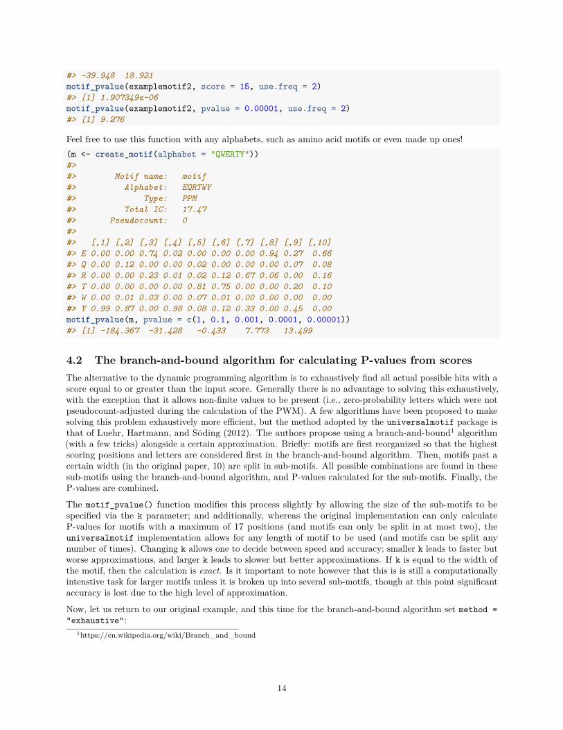
#> -39.948 18.921motif_pvalue(examplemotif2, score = 15, use.freq = 2)#> [1] 1.907349e-06motif_pvalue(examplemotif2, pvalue = 0.00001, use.freq = 2)#> [1] 9.276

Feel free to use this function with any alphabets, such as amino acid motifs or even made up ones!(m <- create_motif(alphabet = "QWERTY"))#>#> Motif name: motif#> Alphabet: EQRTWY#> Type: PPM#> Total IC: 17.47#> Pseudocount: 0#>#> [,1] [,2] [,3] [,4] [,5] [,6] [,7] [,8] [,9] [,10]#> E 0.00 0.00 0.74 0.02 0.00 0.00 0.00 0.94 0.27 0.66#> Q 0.00 0.12 0.00 0.00 0.02 0.00 0.00 0.00 0.07 0.08#> R 0.00 0.00 0.23 0.01 0.02 0.12 0.67 0.06 0.00 0.16#> T 0.00 0.00 0.00 0.00 0.81 0.75 0.00 0.00 0.20 0.10#> W 0.00 0.01 0.03 0.00 0.07 0.01 0.00 0.00 0.00 0.00#> Y 0.99 0.87 0.00 0.98 0.08 0.12 0.33 0.00 0.45 0.00motif_pvalue(m, pvalue = c(1, 0.1, 0.001, 0.0001, 0.00001))#> [1] -184.367 -31.428 -0.433 7.773 13.499

4.2 The branch-and-bound algorithm for calculating P-values from scoresThe alternative to the dynamic programming algorithm is to exhaustively find all actual possible hits with ascore equal to or greater than the input score. Generally there is no advantage to solving this exhaustively,with the exception that it allows non-finite values to be present (i.e., zero-probability letters which were notpseudocount-adjusted during the calculation of the PWM). A few algorithms have been proposed to makesolving this problem exhaustively more efficient, but the method adopted by the universalmotif package isthat of Luehr, Hartmann, and Söding (2012). The authors propose using a branch-and-bound1 algorithm(with a few tricks) alongside a certain approximation. Briefly: motifs are first reorganized so that the highestscoring positions and letters are considered first in the branch-and-bound algorithm. Then, motifs past acertain width (in the original paper, 10) are split in sub-motifs. All possible combinations are found in thesesub-motifs using the branch-and-bound algorithm, and P-values calculated for the sub-motifs. Finally, theP-values are combined.

The motif_pvalue() function modifies this process slightly by allowing the size of the sub-motifs to bespecified via the k parameter; and additionally, whereas the original implementation can only calculateP-values for motifs with a maximum of 17 positions (and motifs can only be split in at most two), theuniversalmotif implementation allows for any length of motif to be used (and motifs can be split anynumber of times). Changing k allows one to decide between speed and accuracy; smaller k leads to faster butworse approximations, and larger k leads to slower but better approximations. If k is equal to the width ofthe motif, then the calculation is exact. Is it important to note however that this is is still a computationallyintenstive task for larger motifs unless it is broken up into several sub-motifs, though at this point significantaccuracy is lost due to the high level of approximation.

Now, let us return to our original example, and this time for the branch-and-bound algorithm set method ="exhaustive":

1https://en.wikipedia.org/wiki/Branch_and_bound

14

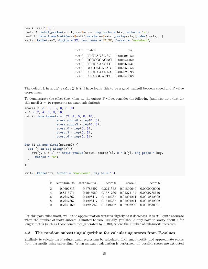
https://en.wikipedia.org/wiki/Branch_and_bound

res <- res[1:6, ]pvals <- motif_pvalue(motif, res$score, bkg.probs = bkg, method = "e")res2 <- data.frame(motif=res$motif,match=res$match,pval=pvals)[order(pvals), ]knitr::kable(res2, digits = 22, row.names = FALSE, format = "markdown")

motif match pvalmotif CTCTAGAGAC 0.001494052motif CCCCGGAGAC 0.001944162motif CTCCAAAGTC 0.001960741motif GCCCAGATAG 0.002255555motif CTCCAAAGAA 0.002823098motif CTCTGGATTC 0.002848363

The default k in motif_pvalue() is 8. I have found this to be a good tradeoff between speed and P-valuecorrectness.

To demonstrate the effect that k has on the output P-value, consider the following (and also note that forthis motif k = 10 represents an exact calculation):scores <- c(-6, -3, 0, 3, 6)k <- c(2, 4, 6, 8, 10)out <- data.frame(k = c(2, 4, 6, 8, 10),

score.minus6 = rep(0, 5),score.minus3 = rep(0, 5),score.0 = rep(0, 5),score.3 = rep(0, 5),score.6 = rep(0, 5))

for (i in seq_along(scores)) {for (j in seq_along(k)) {

out[j, i + 1] <- motif_pvalue(motif, scores[i], k = k[j], bkg.probs = bkg,method = "e")

}}

knitr::kable(out, format = "markdown", digits = 10)

k score.minus6 score.minus3 score.0 score.3 score.62 0.9692815 0.6783292 0.2241568 0.01809649 0.00000000004 0.8516271 0.4945960 0.1581260 0.02271134 0.00097881766 0.7647867 0.4298417 0.1418337 0.02291211 0.00128123928 0.7647867 0.4298417 0.1418337 0.02291211 0.001281239210 0.7649169 0.4299862 0.1419202 0.02293202 0.0012830021

For this particular motif, while the approximation worsens slightly as k decreases, it is still quite accuratewhen the number of motif subsets is limited to two. Usually, you should only have to worry about k forlonger motifs (such as those sometimes generated by MEME), where the number of sub-motifs increases.

4.3 The random subsetting algorithm for calculating scores from P-valuesSimilarly to calculating P-values, exact scores can be calculated from small motifs, and approximate scoresfrom big motifs using subsetting. When an exact calculation is performed, all possible scores are extracted

15

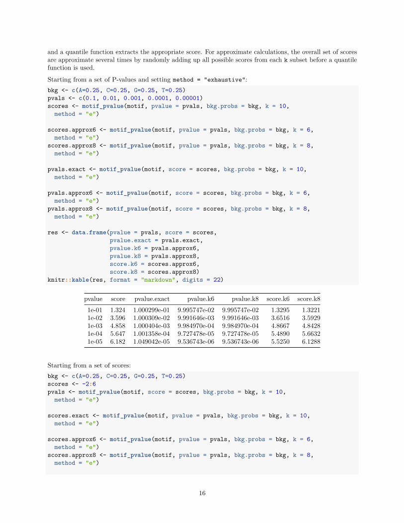
and a quantile function extracts the appropriate score. For approximate calculations, the overall set of scoresare approximate several times by randomly adding up all possible scores from each k subset before a quantilefunction is used.

Starting from a set of P-values and setting method = "exhaustive":bkg <- c(A=0.25, C=0.25, G=0.25, T=0.25)pvals <- c(0.1, 0.01, 0.001, 0.0001, 0.00001)scores <- motif_pvalue(motif, pvalue = pvals, bkg.probs = bkg, k = 10,

method = "e")

scores.approx6 <- motif_pvalue(motif, pvalue = pvals, bkg.probs = bkg, k = 6,method = "e")


pvals.exact <- motif_pvalue(motif, score = scores, bkg.probs = bkg, k = 10,method = "e")

pvals.approx6 <- motif_pvalue(motif, score = scores, bkg.probs = bkg, k = 6,method = "e")


res <- data.frame(pvalue = pvals, score = scores,pvalue.exact = pvals.exact,pvalue.k6 = pvals.approx6,pvalue.k8 = pvals.approx8,score.k6 = scores.approx6,score.k8 = scores.approx8)

knitr::kable(res, format = "markdown", digits = 22)

pvalue score pvalue.exact pvalue.k6 pvalue.k8 score.k6 score.k81e-01 1.324 1.000299e-01 9.995747e-02 9.995747e-02 1.3295 1.32211e-02 3.596 1.000309e-02 9.991646e-03 9.991646e-03 3.6516 3.59291e-03 4.858 1.000404e-03 9.984970e-04 9.984970e-04 4.8667 4.84281e-04 5.647 1.001358e-04 9.727478e-05 9.727478e-05 5.4890 5.66321e-05 6.182 1.049042e-05 9.536743e-06 9.536743e-06 5.5250 6.1288

Starting from a set of scores:bkg <- c(A=0.25, C=0.25, G=0.25, T=0.25)scores <- -2:6pvals <- motif_pvalue(motif, score = scores, bkg.probs = bkg, k = 10,

method = "e")

scores.exact <- motif_pvalue(motif, pvalue = pvals, bkg.probs = bkg, k = 10,method = "e")



16



res <- data.frame(score = scores, pvalue = pvals,pvalue.k6 = pvals.approx6,pvalue.k8 = pvals.approx8,score.exact = scores.exact,score.k6 = scores.approx6,score.k8 = scores.approx8)

knitr::kable(res, format = "markdown", digits = 22)

score pvalue pvalue.k6 pvalue.k8 score.exact score.k6 score.k8-2 4.627047e-01 4.625721e-01 4.625721e-01 -2.000 -1.9840 -2.0092-1 3.354645e-01 3.353453e-01 3.353453e-01 -1.000 -1.0220 -1.00030 2.185555e-01 2.184534e-01 2.184534e-01 0.000 -0.0121 0.00121 1.244183e-01 1.243525e-01 1.243525e-01 1.000 0.9833 1.00242 5.911160e-02 5.907822e-02 5.907822e-02 2.000 2.0029 1.99913 2.163410e-02 2.160931e-02 2.160931e-02 3.000 3.0086 3.00304 5.360603e-03 5.347252e-03 5.347252e-03 4.000 4.0094 3.99625 7.162094e-04 7.152557e-04 7.152557e-04 5.000 4.9790 5.02156 2.193451e-05 2.193451e-05 2.193451e-05 6.057 5.6272 5.9633

As you may have noticed, results from exact calculations are not quite exact. This is due to theuniversalmotif package rounding off values internally for speed.

Session info#> R version 4.1.2 (2021-11-01)#> Platform: x86_64-pc-linux-gnu (64-bit)#> Running under: Ubuntu 20.04.3 LTS#>#> Matrix products: default#> BLAS: /home/biocbuild/bbs-3.14-bioc/R/lib/libRblas.so#> LAPACK: /home/biocbuild/bbs-3.14-bioc/R/lib/libRlapack.so#>#> locale:#> [1] LC_CTYPE=en_US.UTF-8 LC_NUMERIC=C#> [3] LC_TIME=en_GB LC_COLLATE=C#> [5] LC_MONETARY=en_US.UTF-8 LC_MESSAGES=en_US.UTF-8#> [7] LC_PAPER=en_US.UTF-8 LC_NAME=C#> [9] LC_ADDRESS=C LC_TELEPHONE=C#> [11] LC_MEASUREMENT=en_US.UTF-8 LC_IDENTIFICATION=C#>#> attached base packages:#> [1] stats4 stats graphics grDevices utils datasets methods#> [8] base#>#> other attached packages:#> [1] cowplot_1.1.1 dplyr_1.0.8 ggtree_3.2.1

17

#> [4] ggplot2_3.3.5 MotifDb_1.36.0 GenomicRanges_1.46.1#> [7] Biostrings_2.62.0 GenomeInfoDb_1.30.1 XVector_0.34.0#> [10] IRanges_2.28.0 S4Vectors_0.32.3 BiocGenerics_0.40.0#> [13] universalmotif_1.12.4#>#> loaded via a namespace (and not attached):#> [1] MatrixGenerics_1.6.0 Biobase_2.54.0#> [3] tidyr_1.2.0 jsonlite_1.8.0#> [5] assertthat_0.2.1 highr_0.9#> [7] yulab.utils_0.0.4 GenomeInfoDbData_1.2.7#> [9] Rsamtools_2.10.0 yaml_2.3.5#> [11] pillar_1.7.0 lattice_0.20-45#> [13] glue_1.6.2 digest_0.6.29#> [15] colorspace_2.0-3 ggfun_0.0.5#> [17] htmltools_0.5.2 Matrix_1.4-0#> [19] XML_3.99-0.9 pkgconfig_2.0.3#> [21] bookdown_0.24 zlibbioc_1.40.0#> [23] purrr_0.3.4 tidytree_0.3.8#> [25] patchwork_1.1.1 scales_1.1.1#> [27] ggplotify_0.1.0 BiocParallel_1.28.3#> [29] tibble_3.1.6 generics_0.1.2#> [31] farver_2.1.0 ellipsis_0.3.2#> [33] withr_2.4.3 SummarizedExperiment_1.24.0#> [35] lazyeval_0.2.2 cli_3.2.0#> [37] splitstackshape_1.4.8 magrittr_2.0.2#> [39] crayon_1.5.0 evaluate_0.15#> [41] fansi_1.0.2 nlme_3.1-155#> [43] MASS_7.3-55 tools_4.1.2#> [45] data.table_1.14.2 BiocIO_1.4.0#> [47] lifecycle_1.0.1 matrixStats_0.61.0#> [49] stringr_1.4.0 aplot_0.1.2#> [51] munsell_0.5.0 DelayedArray_0.20.0#> [53] compiler_4.1.2 gridGraphics_0.5-1#> [55] tinytex_0.37 rlang_1.0.1#> [57] grid_4.1.2 RCurl_1.98-1.6#> [59] rjson_0.2.21 labeling_0.4.2#> [61] bitops_1.0-7 rmarkdown_2.11#> [63] restfulr_0.0.13 gtable_0.3.0#> [65] DBI_1.1.2 R6_2.5.1#> [67] GenomicAlignments_1.30.0 knitr_1.37#> [69] rtracklayer_1.54.0 fastmap_1.1.0#> [71] utf8_1.2.2 treeio_1.18.1#> [73] ape_5.6-1 stringi_1.7.6#> [75] parallel_4.1.2 Rcpp_1.0.8#> [77] vctrs_0.3.8 tidyselect_1.1.2#> [79] xfun_0.29

ReferencesBhattacharyya, A. 1943. “On a Measure of Divergence Between Two Statistical Populations Defined by TheirProbability Distributions.” Bulletin of the Calcutta Mathematical Society 35: 99–109.

Grant, C.E., T.L. Bailey, and W.S. Noble. 2011. “FIMO: Scanning for Occurrences of a Given Motif.”Bioinformatics 27: 1017–8.

18

Gupta, S., J.A. Stamatoyannopoulos, T.L. Bailey, and W.S. Noble. 2007. “Quantifying Similarity BetweenMotifs.” Genome Biology 8: R24.

Hellinger, Ernst. 1909. “Neue Begründung Der Theorie Quadratischer Formen von Unendlichvielen Veränder-lichen.” Journal Für Die Reine Und Angewandte Mathematik 136: 210–71.

Kullback, S., and R. A. Leibler. 1951. “On Information and Sufficiency.” The Annals of MathematicalStatistics 22: 79–86.

Luehr, S., H. Hartmann, and J. Söding. 2012. “The XXmotif Web Server for EXhaustive, Weight MatriX-Based Motif Discovery in Nucleotide Sequences.” Nucleic Acids Research 40: W104–W109.

Mahony, S., P.E. Auron, and P.V. Benos. 2007. “DNA Familial Binding Profiles Made Easy: Comparison ofVarious Motif Alignment and Clustering Strategies.” PLoS Computational Biology 3 (3): e61.

Roepcke, S., S. Grossmann, S. Rahmann, and M. Vingron. 2005. “T-Reg Comparator: An Analysis Tool forthe Comparison of Position Weight Matrices.” Nucleic Acids Research 33: W438–W441.

Sandelin, A., and W.W. Wasserman. 2004. “Constrained Binding Site Diversity Within Families ofTranscription Factors Enhances Pattern Discovery Bioinformatics.” Journal of Molecular Biology 338 (2):207–15.

Wang, T., and G.D. Stormo. 2003. “Combining Phylogenetic Data with Co-Regulated Genes to IdentifyMotifs.” Bioinformatics 19 (18): 2369–80.

19

motif comparisons and p-values - bioconductor

Documents