1

Mosaic Brains? A Methodological Critique of Joel et al. (2015)

Online document – December 23, 2015

Marco Del Giudice, University of New Mexico (marcodg@unm.edu) Richard A. Lippa, California State University, Fullerton

David A. Puts, Pennsylvania State University Drew H. Bailey, University of California, Irvine

J. Michael Bailey, Northwestern University David P. Schmitt, Bradley University

In their recent and widely publicized paper, Joel et al. (2015) made two main empirical claims. First, they claimed that the brains of individual males and females show very little internal consistency in their combination of “male-typical” and “female-typical” features, e.g.:

“Our results demonstrate that even when analyses are restricted to a small number of brain regions (or connections) showing the largest sex/gender differences, internal consistency is rare and is much less common than substantial variability (i.e., being at the one end of the “maleness-femaleness” continuum on some elements and at the other end on other elements)” (p. 15472). Second, they claimed that the overlap between male and females in the distribution of

anatomical traits in specific brain regions is so large that it calls into question the very idea of gender differences in brain structure, e.g.:

“This extensive overlap undermines any attempt to distinguish between a “male” and a “female” form for specific brain features” (p. 15471). The first claim was based on a novel method for assessing internal consistency, which

consists in the following procedure: (a) from a larger dataset, select a small number of variables (7-12 in Joel et al.’s paper) showing the largest gender differences; (b) for each individual, count the number of variables (or “features”) whose value falls in the extreme 33% of the male or female distribution; (c) classify an individual as “internally consistent” if all of the variables fall in the same category (“male-end”, “female-end”, or “intermediate”); and (d) classify an individual as showing “substantial variability” if he/she has at least one male-end variable and one female-end variable.

2

The validity of this method is questionable on several grounds. To begin with, the method capitalizes on chance by selecting the variables with the largest effect sizes. It also discards most of the information in those variables by reducing them to three categories, a problematic and potentially misleading practice (e.g., Altman & Royston, 2006; MacCallum, Zhang, Preacher, & Rucker, 2002). Most importantly, the method employs an unrealistically strict criterion for “internal consistency” coupled with a lax criterion for “substantial variability.” As an example, consider a fictional male—Max—who is rated on a number of sex-typical preferences for leisure activities: boxing, construction, playing golf, scrapbooking, using cosmetics, and playing video games (see the supplementary material in Joel et al., 2015, p. 8). Max has no interest in scrapbooking or cosmetics but is passionate about boxing, golf, and construction; however, he does not like video games. By the standards of Joel et al.’s method, this profile would be classified as “substantially variable” and presented as evidence that Max shows a “mosaic” of male-typical and female-typical features.

More generally, it is clear that Joel et al.’s method will only detect consistency if the

variables selected for the analysis show extremely high correlations with each other. Indeed, the correlations required to detect consistency might fall outside the range of values that can be realistically expected in empirical data on gender differences, whether in behavior or brain structure.

The second claim in Joel et al. (2015) concerns the overlap between male and female

distributions. While it is true that there is considerable male-female overlap in each individual brain feature (although the overlap may be inflated by measurement error), the combined effect of gender differences across multiple variables is often much larger than that of the individual variables. The overall amount of between-group overlap on a set of variables can be easily estimated with multivariate effect sizes (see Del Giudice, 2009, 2013; Del Giudice, Booth, & Irwing, 2012).

In this critique, we evaluate the claims made by Joel et al. (2015) by taking a closer look

at their methodology. First, we used simulations to explore the validity of Joel et al.’s method, by systematically varying the size of gender differences and correlations between variables. We found that, under realistic conditions, Joel et al.’s method almost always returns the same pattern of results—that is, very low proportions of “internally consistent” profiles and much higher proportions of “substantially variable” profiles. More strikingly, the proportion of “internally consistent” male-typical and female-typical profiles detected by Joel et al.’s method remains very low (less than about 10%) even when all the variables show large sex differences (more than one standard deviation) and are almost perfectly correlated with one another (r = .90). Thus, our results show that the method has poor validity, and should not be used to draw conclusions about internal consistency in males and females.

3

Given our concerns about the method’s validity, we decided to test it in different domain, that of anatomical differences between species. In particular, we used real-world data on the facial morphology of three species of monkeys from different genera (Fig. 1). This is an interesting test case because these anatomical differences (a) are larger than gender differences and (b) reflect unambiguous biological distinctions. Would the method be able to detect internal consistency when applied to these data? As it turns out, the answer is no. Even if differences between species were extremely large (about 4 to 5.5 standard deviations, on average) and there was virtually no overlap between distributions, the method found only a small minority of individuals with “internally consistent” species-typical facial features (from 1.1% to 5.1%). This empirical reductio ad absurdum further demonstrates that the method lacks validity, and should not be expected to return interpretable results when applied to the study of gender differences.

Fig. 1. The three monkey species examined in the morphological analysis (Picture credits, A: Sakurai Midori; B: Ron Waddington; C: Dario Sanches. Creative Commons BY-SA 2.0). Finally, we addressed Joel et al.’s second point by estimating the multivariate overlap

between males and females, using the same variables analyzed by the authors in the original paper. In six brain imaging datasets, the overlap between male and female distributions ranged from 30% to 58%, with a mean of 42%. These figures are consistent with the idea that the brains of males and females show at least moderate anatomical overlap (indeed, we are aware of no claims to the contrary in the literature). However, they are at odds with Joel et al.’s implication that the overlap is so large as to invalidate the very idea of gender differences in brain structure.

To further explore this issue, we used linear discriminant analysis (LDA) to classify

individuals as male or female based on their brain structure. Depending on the dataset, we were able to correctly identify an individual’s gender about 69%-77% of the time (mean = 72.9%). These values still underestimate the predictive power of brain structure, as each dataset only considers one aspect of brain anatomy (volume, thickness, etc.). Combining different sources of information would likely improve prediction further. Taken together, these results suggest that it is reasonable to speak of a maleness-femaleness continuum in brain structure when variables are aggregated with appropriate multivariate methods.

4

1. Simulations

In the simulations, samples of N = 500,000 individuals (50% females) were generated

from a multivariate normal distribution of K variables, with K = 7 and 12 (the minimum and maximum number of variables in Joel et al.’s analyses). The univariate effect size of gender differences was the same for all the variables and ranged from d = .50 to d = 1.25 in steps of .25 (roughly corresponding to the range of average d values in the datasets analyzed by Joel et al.; see the supplementary information in Joel et al., 2015). Correlations were the same between all the variables, and ranged from .00 to .90 in steps of .025. Joel et al.’s method was applied as described above, using the 33rd/67th percentiles of the male/female distributions as cutoffs. Simulations were carried out in RTM 3.2 (R Core Team, 2015).

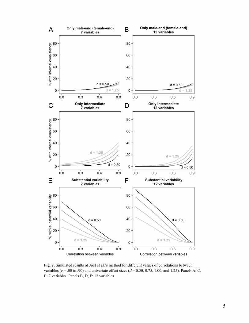
Simulation results are shown in Fig. 2. The proportion of consistent male-end and

female-end profiles remains low in all conditions (Fig. 2A and 2B), and actually decreases slightly as gender differences become larger (larger values of d). The proportion of consistent “intermediate” profiles is also low (but typically larger than that of consistent gender-typical profiles) unless correlations and/or gender differences become extremely large (Fig. 2C and 2D). Finally, the method returns many “substantially variable” profiles unless correlations and/or gender differences become extremely large (Fig. 2E and 2F). (Note: the figure does not show the proportions of profiles that are neither internally consistent nor substantially variable.)

Some of the simulated scenarios are intentionally unrealistic. For example, an average

correlation of .90 is not expected in most real-world datasets. Similarly, datasets showing an average male-female difference of more than one standard deviation are extremely rare (among the datasets analyzed by Joel et al., this happened only for sex-typical leisure/occupational preferences). In most domains, a realistic range of values would include average correlations between r = .30 and r = .60 and average effect sizes between d = 0.50 and d = 1.00 (absolute values). Within this range, Joel et al.’s method nearly always returns the same pattern of results—a preponderance of “substantially variable” profiles, a minority of “intermediate” profiles, and a very small proportion (often close to zero) of “gender-typical” profiles (Fig. 2). It is not surprising that Joel et al. (2015) found this pattern in their analyses. Our simulations show that this pattern of results is expected under most realistic conditions; in particular, the proportion of “internally consistent” gender-typical profiles provides very little information about the actual consistency of male and female characteristics.

5

Fig. 2. Simulated results of Joel et al.’s method for different values of correlations between variables (r = .00 to .90) and univariate effect sizes (d = 0.50, 0.75, 1.00, and 1.25). Panels A, C, E: 7 variables. Panels B, D, F: 12 variables.

% w

ith in

tern

al c

onsi

sten

cy

0

20

40

60

80

0.0 0.3 0.6 0.9

d = 0.50

d = 1.25 0

20

40

60

80

0.0 0.3 0.6 0.9

d = 0.50

d = 1.25

% w

ith in

tern

al c

onsi

sten

cy

0

20

40

60

80

0.0 0.3 0.6 0.9

d = 0.50

d = 1.25

0

20

40

60

80

0.0 0.3 0.6 0.9d = 0.50

d = 1.25

Correlation between variables

% w

ith s

ubst

antia

l var

iabi

lity

0

20

40

60

80

0.0 0.3 0.6 0.9

d = 0.50

d = 1.25

Correlation between variables

0

20

40

60

80

0.0 0.3 0.6 0.9

d = 0.50

d = 1.25

A B

C D

E F

Only male-end (female-end) 7 variables

Only male-end (female-end) 12 variables

Only intermediate 7 variables

Only intermediate 12 variables

Substantial variability 12 variables

Substantial variability 7 variables

6

2. Facial Morphology in Monkeys

To test the performance of Joel et al.’s method in a domain showing large and

unambiguous differences, we obtained a real-world dataset of facial morphology in three species of monkeys (Fig. 1): Macaca fascicularis (crab-eating macaque; 59 individuals), Cercopithecus aethiops (grivet; 20 individuals), and Cebus apella (tufted capuchin; 31 individuals). The morphological data were kindly provided by Joan Richtsmeier; for a detailed description of the dataset see Corner and Richtsmeier (1991) and Richtsmeier et al. (1993a, 1993b). The dataset includes 20 three-dimensional cranial landmarks for each individual.

For the purposes of this analysis, we calculated 190 distances between the 20 landmarks

of each individual monkey. To limit the effect of gross differences in cranial size (a conservative approach), we first equalized the minimum and maximum values of X, Y, and Z coordinates for the three species (results were virtually identical with or without equalization). For each pairwise comparison between species, we selected the 7 distances showing the largest species differences (thus mimicking the selection approach of Joel et al.). We then applied Joel et al.’s method as described above. Analyses were carried out in RTM 3.2.

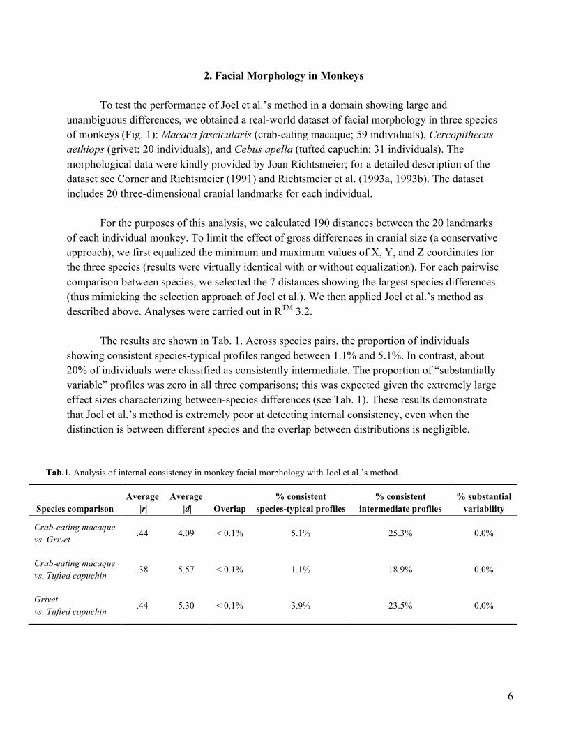
The results are shown in Tab. 1. Across species pairs, the proportion of individuals

showing consistent species-typical profiles ranged between 1.1% and 5.1%. In contrast, about 20% of individuals were classified as consistently intermediate. The proportion of “substantially variable” profiles was zero in all three comparisons; this was expected given the extremely large effect sizes characterizing between-species differences (see Tab. 1). These results demonstrate that Joel et al.’s method is extremely poor at detecting internal consistency, even when the distinction is between different species and the overlap between distributions is negligible.

Tab.1. Analysis of internal consistency in monkey facial morphology with Joel et al.’s method.

Species comparison Average

|r| Average

|d| Overlap % consistent

species-typical profiles % consistent

intermediate profiles % substantial

variability

Crab-eating macaque vs. Grivet

.44 4.09 < 0.1% 5.1% 25.3% 0.0%

Crab-eating macaque vs. Tufted capuchin .38 5.57 < 0.1% 1.1% 18.9% 0.0%

Grivet vs. Tufted capuchin .44 5.30 < 0.1% 3.9% 23.5% 0.0%

7

3. Male-Female Overlap in Joel et al.’s Brain Imaging Data

To estimate the amount of male-female overlap in the brain imaging data analyzed by

Joel et al., we computed multivariate effect sizes (Mahalanobis D) as described in Del Giudice (2009, 2013). D is the multivariate equivalent of Cohen’s d and has the same interpretation in terms of distribution overlap. As an index of overlap we used Cohen’s 1-U1, the proportion of overlap over the joint distribution of two groups. This is the most commonly reported overlap index in the psychological literature (see Del Giudice, 2009). Confidence intervals on D were computed with bias-corrected and accelerated bootstrap (10,000 samples; see Kelley, 2005), and male-female overlap was estimated from D assuming multivariate normality. Analyses were performed in RTM 3.2.

The brain imaging datasets were kindly provided by Daphna Joel. We reanalyzed six out

of seven datasets (the DTI connectivity dataset was in a format that we were unable to interpret). To maximize comparability with the findings by Joel et al., we computed D using the same variables selected by the authors within each dataset. Prior to computing D, we checked the similarity between male and female correlation matrices using Tucker’s congruence coefficient (CC; see Abdi, 2007). Congruence was very high in all datasets (CC between .95 and .99).

The results are shown in Tab. 2. Values of D ranged from 0.69 to 1.47 (average 1.10).

The corresponding male-female overlap ranged from 30% to 58%, with a mean of 42%. In five out of six datasets, the overlap was less than 50%, indicating that the separation between male and female distributions was larger than their overlap. In total, these data show a moderate amount of overlap in brain structure between males and females, at least when using the variables selected by Joel et al. (2015). Note that these estimates of D are likely to be inflated by capitalization on chance in variable selection (see above) and deflated by measurement error in the anatomical variables.

Tab.2. Multivariate effect sizes and overlap coefficients for six brain imaging datasets in Joel et al. (2015).

Dataset Average |r| D 95% CI Overlap

1000, VBM, 18-26 subsample .29 0.89 [0.69; 1.02] 49%

1000, VBM .43 0.92 [0.74; 1.03] 48%

First, VBM .39 1.38 [1.07; 1.55] 33%

DTI fractional anisotropy .47 1.25 [0.69; 1.44] 36%

NKI, SBA, cortical thickness .51 0.69 [0.36; 0.86] 58%

NKI, SBA, volume .45 1.47 [1.09; 1.65] 30%

8

Another caveat to the present analysis is that the datasets are relatively small, which is

expected to result in upward-biased values of D (again because of capitalization on chance). As a rule of thumb for minimizing bias on D, Del Giudice (2013) recommended a ratio of at least 100 cases per variable. The ratio of cases to variables in the present datasets ranged from 12.5 (DTI fractional anisotropy) to 85.5 (1000, VBM). This is one more reason why these estimates should not be taken out of context, but only used to evaluate Joel et al.’s claims against their own data. Accurate estimates of the overall male-female overlap in brain structure will require both larger datasets and more information on the reliability of brain structure measures.

To gain further perspective on Joel et al.’s brain imaging data, we performed a series of

linear discriminant analyses to predict gender based on brain structure using the full datasets. We used PCA to reduce the number of variables and avoid collinearity; in each dataset, we extracted enough components to explain 80% of the variance. The proportion of correct classifications was computed with the leave-one-out method. Correct classifications ranged from 68.5% to 77.2% (mean = 72.9%; all p’s < .001). When using only the variables selected by Joel et al., correct classifications dropped to 62.9%-75.0% (mean = 68.6; all p’s < .001). The main limitation of this approach is that each dataset only contains information about one aspect of brain structure. We anticipate that combining multiple sources of brain imaging data (e.g., volume, thickness, connectivity) would make it possible to identify a person’s gender from his/her brain structure with considerable accuracy.

References Abdi, H. (2007). RV coefficient and congruence coefficient. In N. Salkind (Ed.), Encyclopedia of

measurement and statistics (pp. 849-853). Thousand Oaks, CA: Sage. Altman, D. G., & Royston, P. (2006). The cost of dichotomising continuous variables. BMJ, 332,

1080. Corner, B. D., & Richtsmeier, J. T. (1991). Morphometric analysis of craniofacial growth in

Cebus apella. American Journal of Physical Anthropology, 84, 323-342. Del Giudice, M. (2009). On the real magnitude of psychological sex differences. Evolutionary

Psychology, 7, 264-279. Del Giudice, M. (2013). Multivariate misgivings: Is D a valid measure of group and sex

differences? Evolutionary Psychology, 11, 1067-1076. Del Giudice, M., Booth, T., & Irwing, P. (2012). The distance between Mars and Venus:

Measuring global sex differences in personality. PLoS ONE, 7, e29265. Joel, D., Berman, Z., Tavor, I., Wexler, N., Gaber, O., Stein, Y., et al. (2015). Sex beyond the

genitalia: The human brain mosaic. PNAS, 112, 15468-15473. Kelley, K. (2005). The effects of nonnormal distributions on confidence intervals around the

standardized mean difference: Bootstrap and parametric confidence intervals. Educational and Psychological Measurement, 65, 51-69.

9

MacCallum, R. C., Zhang, S., Preacher, K. J., & Rucker, D. D. (2002). On the practice of dichotomization of quantitative variables. Psychological Methods, 7, 19-40.

R Core Team (2015). R: A language and environment for statistical computing. R Foundation for Statistical Computing, Vienna, Austria. URL: https://www.R-project.org/.

Richtsmeier, J. T., Cheverud, J. M., Danahey, S. M., Corner, B. C., & Lele, S. (1993a). Sexual dimorphism of ontogeny in the crab eating macaque (Macaca fascicularis). Journal of Human Evolution, 25, 1-30.

Richtsmeier, J. T., Corner, B. D., Grausz, H. M., Cheverud, J. M, & Danahey, S. (1993b). The role of postnatal growth pattern in the production of facial morphology. Systematic Biology, 42, 307-330.