mortgage case studies - lawrence berkeley national laboratory
TRANSCRIPT

Impact of Energy Use and Price Variations on Default Risk in
Commercial Mortgages: Case Studies
26 September 2017
Paul Mathew Kaiyu Sun
Baptiste Ravache Lawrence Berkeley National Laboratory
Paulo Issler
Nancy Wallace University of California, Berkeley

1
Disclaimer This document was prepared as an account of work sponsored by the United States Government. While this document is believed to contain correct information, neither the United States Government nor any agency thereof, nor The Regents of the University of California, nor any of their employees, makes any warranty, express or implied, or assumes any legal responsibility for the accuracy, completeness, or usefulness of any information, apparatus, product, or process disclosed, or represents that its use would not infringe privately owned rights. Reference herein to any specific commercial product, process, or service by its trade name, trademark, manufacturer, or otherwise, does not necessarily constitute or imply its endorsement, recommendation, or favoring by the United States Government or any agency thereof, or The Regents of the University of California. The views and opinions of authors expressed herein do not necessarily state or reflect those of the United States Government or any agency thereof or The Regents of the University of California

2
Acknowledgements
This work was supported by the Assistant Secretary for Energy Efficiency and Renewable Energy, Building Technologies Program, of the U.S. Department of Energy under Contract No. DE-AC02-05CH11231. The authors gratefully acknowledge the following individuals and organizations for participating in this pilot project:
• Keith Hanley, Silicon Valley Bank • Michael O’Neill, Colorado Lending Source • Dennis Williams, Northmarq
The authors gratefully acknowledge Jason Hartke, Holly Carr, and Cindy Zhu at the U.S. Department of Energy for their sponsorship and guidance of this project. The authors thank the project team members who provided input for this report, particularly Philip Coleman and Jeff Deason at Lawrence Berkeley National Laboratory.

3
TABLE OF CONTENTS
Executive Summary ....................................................................................................... 4
1 Introduction and Background ................................................................................. 6
2 Approach ................................................................................................................... 7
3 Denver Office ............................................................................................................ 93.1 Energy model overview .................................................................................................... 93.2 Source EUI variations and default risk ........................................................................... 103.3 Electricity price variations and default risk for Denver region ........................................ 12
4 Sonoma Office ........................................................................................................ 144.1 Energy model overview .................................................................................................. 144.2 Source EUI variations and default risk ........................................................................... 164.3 Electricity price variations and default risk for Northern California ................................. 18
5 San Jose Office ...................................................................................................... 205.1 Energy model overview .................................................................................................. 205.2 Source EUI variations and default risk ........................................................................... 22
6 Denver Hotel ........................................................................................................... 256.1 Energy model overview .................................................................................................. 256.2 Source EUI variations and default risk ........................................................................... 27
7 San Francisco Multi-family Building .................................................................... 307.1 Energy model overview .................................................................................................. 307.2 Source EUI variations and default risk ........................................................................... 32
8 Conclusions and Recommendations ................................................................... 35
9 References .............................................................................................................. 37

4
Executive Summary This report documents the impact of energy use and price variations on commercial mortgage default risk in five buildings: an office building in the Denver area, two office buildings in northern California, a hotel in the Denver area, and a multi-family residential building in San Francisco. We used parametric energy simulation to analyze the impact of variations in operational practices on source energy use intensity (EUI). We then computed the impact of source EUI variations on default risk using coefficients from an empirical logistic regression model developed earlier in this research effort as documented in Wallace et al. [2017]. Table 1 shows the relative range of variation in source EUI and default risk for each building. The table also shows the default rate variation relative to the TREPP average default rate of 800 basis points (8%).
Table 1. Range of variation in source EUI and default risk for five case studies.
Building Source EUI variation (%) Default rate variation (bp)
Default rate variation relative to 8% avg. (TREPP)
Denver Office -54% to +132% -248 to +268 -31% to +34% Sonoma Office -40% to +183% -161 to +331 -20% to +41% San Jose Office -62% to +119% -308 to +249 -39% to +31% Denver Hotel -11% to +17% -37 to +49 -5% to +6% San Francisco Multi-family -20% to +26% -72 to +74 -9% to +9%
To summarize, we found that variations in energy use that are reasonably common could raise or lower the default rates in these properties by between roughly 5% and 40%, depending on the property type and geography. This is a fairly significant potential impact, especially given our prior finding that the industry generally does not take energy usage into consideration in assessing loans [Mathew et al., 2016]. We also computed the impact of electricity price variations in the Denver area and northern California using variations of wholesale electricity prices and calculated the corresponding relative range of variation in default risk (Table 2).
Table 2. Range of variation in default risk based on wholesale electricity prices for the Denver area and northern California.
Wholesale price region Default rate variation (bp)
Default rate variation relative to TREPP avg (%)
Denver area +159 to +501 +20% to +63% Northern California -49 to +705 -6% to +88%
Similar to energy usage, variation in electricity pricing appears to have a substantial effect on default risk in these two markets, with an increased default risk (again, from the TREPP average of 8%) ranging as high as roughly 60% in the Denver area and nearly 90% in northern California. Energy prices were also not found to be a prominent factor among lenders we have surveyed. Given the methodological limitations of the study, these results should be seen as indicative of the default risks, rather than precise estimates of default rate for a given building.

5
We presented and discussed these findings with each of the three lender organizations that provided the data for these case studies. All three lenders indicated that these findings are meaningful, i.e., that the range of default risk variations are material. One lender noted that he had never previously given any thought to energy costs and risks and that these results suggested that his company should consider them in the loan process. We also discussed potential approaches to effectively factoring energy costs and risks into the underwriting process. Based on these discussions with lenders and other stakeholders, we recommend the following (in the near term):
• Lenders should request an estimate of energy cost variations as part of the loan application. This may be based on historical utility bill data or more in-depth analysis if that is available. This will at a minimum provide lenders a range of variation that they can factor into the NOI analysis. More broadly from a market transformation standpoint, it will signal to owners that energy costs matter to the lender.
• Develop a simple-to-use energy risk score that can be used for underwriting, analogous to the seismic risk score. Notably, the lenders indicated that they would be willing to pilot such a score on new loans.

6
1 Introduction and Background This report documents five case studies on the impact of energy use and price variations on commercial mortgage default risk. These case studies are part of a larger project on evaluating the impact of energy factors on commercial real estate lending. The first part of the project analyzed the effects of building-level energy consumption and the time-series risk of energy prices on the default risk of commercial mortgages based on a unique data set that merges the building-level energy use data collected through the benchmarking ordinances of six cities with origination and performance data for commercial mortgages that have been securitized into commercial mortgage backed securities (CMBS). We used these data to develop a logistic regression model relating default risk to source energy use intensity (EUI) and electricity prices as well as other dependent variables. We found that building source EUI and “electricity price gap”1 are statistically and economically associated with commercial mortgage defaults. The findings are documented in a report entitled “Impact of Energy Factors on Default Risk in Commercial Mortgages” [Wallace et al. 2017]. The applicability of these results to a specific loan for a specific building is dependent on the context and characteristics of the subject building. From an underwriting perspective, the ensuing issue is to understand the default risk implications for individual loans, i.e., how do energy use and price in a specific building affect the default risk on its mortgage? Additionally, a key goal of the overall project is to engage and work with lenders to assess the implications of these research findings on their underwriting policies and practices. Toward that end, we collaborated with three lender organizations - Colorado Lending Source, Northmarq, and Silicon Valley Bank - to analyze specific buildings in their respective loan portfolios. We analyzed a total of five buildings. For each case, we applied the results from the earlier study to show how variations in energy use and price affect default risk, taking into account the specific building characteristics and context for each. This report is organized as follows:
• Section 2 describes the analysis approach. • Sections 3-7 present results each of the five case studies. For each, we present:
o key building characteristics and simulated energy use; o parameters varied to simulate good, average and poor operational practice; o default risk variations due to source EUI and variations; and o default risk variations due to electricity price variations.
• Section 8 makes recommendations on how to incorporate energy factors into the underwriting process.
1 Electricity price gap is a unique measure we developed, computed as the difference between realized and expected electricity prices since the date of loan origination.

7
2 Approach For each building, we calculate two end results:
● default risk variation due to source EUI variations, and ● default risk variation due to electricity price variations.
We used the following approach to compute default risk variations due to source EUI variations:
● Compile available physical and operational characteristics for each building. We used information ordinarily collected and generated as part of the mortgage process (e.g., appraisals, property condition assessments) or easily available via public sources (e.g., Google Earth)
● Develop an EnergyPlus building energy simulation model based on the available information. The model accounted for: building geometry, HVAC type (central plant vs. distributed), window size and location, and assumptions of building envelope, HVAC, and lighting efficiency based on year of construction. Most other parameters (e.g., occupancy schedules, etc.) were defaulted to ”typical” values drawn from the DOE reference building models2.
● Compare the modeled energy use against actual energy use of the building, if available, for reasonableness. If actual energy data were not available, we compared the simulated values with measured data from similar buildings in the DOE Building Performance Database (BPD)3.
● Define a list of operational parameters that have the largest impact on source EUI. The list of parameters were based on prior studies and edited based on the features of each building. For example, the hotel building included a parameter to account for different levels of vacancy. It should be noted that the list of operations parameters modeled was not comprehensive and there are any number of additional operational parameters that affect energy use but were not part of this analysis, due to modeling limitations or scope.
● For each operational parameter, define three levels of practice: good, average and poor. Good practice represents design intent or optimal performance of the building. For average and poor practice, the analysis assumes the building has the capability to run at the good practice level, but runs less efficiently due to poorer facility management or occupant behavior.
● Run the parametric simulations to obtain range of source EUI variations due to different levels of practice. First, we simulated good and poor levels of practice for each parameter keeping all other parameters at the average level of practice. This provided the range of variation due to each variable. Next we modeled scenarios where groups of parameters were characterized by good or poor practice, including extreme cases where all were good or poor. This provided an overall range of source EUI variation. If actual energy use was available, we applied the relative (%) source EUI variations from the simulation results to actual energy use. If not available, we just used the simulated source EUI values.
2 https://energy.gov/eere/buildings/commercial-reference-buildings 3 https://bpd.lbl.gov/

8
● Compute default risk variations due to source EUI variations. We used the variable coefficients from the default risk logistic regression model to calculate the change in default risk due to the change in source EUI.
We computed the default risk variation due to electricity price as follows:
● Compile electricity price data for five-year period. Our intent was to obtain five years of data starting at the mortgage origination date. However, due to limitations in data availability, we were not able to do this and instead used data that were as close as possible to the mortgage origination.
● Simulate 10,000 electricity price paths based on forward market prices. ● Calculate electricity price gap for each simulated path, following the methodology
documented in the companion technical report [Wallace et al. 2017]. ● Generate a probability distribution of the electricity price gap at the end of year five. ● Calculate the default risk variation due to the variation in electricity price gap. We used
the variable coefficients from the default risk logistic regression model to calculate the change in default risk due to the change in electricity price gap.
Sections 3-7 below present the five case studies. For data privacy, the buildings are not identified by name or address. Section 8 concludes and proposes recommendations based on discussions with the lenders.

9
3 Denver Office
3.1 Energy model overview
This building, located in the Denver metropolitan area, has a gross floor area of 48,000 sf comprising 38,000 sf of office space and 10,000 sf of warehouse space. The building has two stories with a rectangular floor plate, as shown in Figure 1. It was constructed in 2000. The HVAC system is packaged rooftop units. The building also includes a rooftop solar PV system. The mortgage loan was funded in February 2011.
Figure 1. Simulation model geometry of Denver office building.
The total source energy (electricity and natural gas) for the baseline model was 6070 MMBtu. Figure 2 shows the energy use breakout from the baseline simulation model.
Figure 2. Simulated source energy end uses for Denver office building.
HVAC50%
Ligh-ng33%
Plugloads17%
DenverOfficeSourceEnergyEndUses

10
The appraisal report did not include any historical energy use information. Separately, we obtained utility bills for 20164 and calculated total source energy using the same site-source conversion factors as used for the simulation model. The bill-based total source energy is 6,178 MMBtu, which is within 2% of the simulation-based source energy – very well within the range of reasonableness for this purpose – i.e., to compute relative variations in source EUI.
3.2 Source EUI variations and default risk
Table 3 below shows the levels of practice for various operational parameters used to compute source EUI variations. Note that for occupant density and plug load density, ”good” means low density and “poor” means high density.
Table 3. Range of practice for various operations parameters used for computing source EUI variations for Denver office building
Factor Good practice Average practice Poor practice Lighting controls Daylight-dimming + occ sensor Occ sensor only Timer only
Plug load controls Turn off when occupants leave Sleep mode by itself No energy saving measures Plug load intensity 0.4 W/sf 0.75 W/sf 2.0W/sf Occupant density 400 sf/person 200 sf/person 130 sf/person
Occupant schedule 8 hour workday 12 hour workday 16 hour workday HVAC schedule optimal start 2hr +/- Occupant schedule n/a
Thermostat settings 68°F heating, 78°F cooling Setback: 60°F - 85°F
70°F heating, 76°F cooling Setback: 68°F - 80°F
72°F heating, 74°F cooling No setback
Supply air temp reset Reset based on warmest zones Reset based on stepwise
function of outdoor air temperature
Constant supply air temperature
VAV box min flow settings 15% of design flow rate 30% of design flow rate 50% of design flow rate
Economizer controls Enthalpy Dry bulb none/broken Figure 3 shows the resulting source EUI variations for each parameter, expressed relative to average practice. Plug load density, lighting control, thermostat settings and occupancy schedules show the greatest range.
4 The utility bills were not available for two months. Energy use for these months was interpolated.

11
Figure 3. Simulated relative source EUI variations due to poor and good operational practices
for Denver office building. Values are relative to average practice.
We then computed the source EUI variations for scenarios that represented various combinations of practice levels. The parameters were grouped into two categories:
● Facilities management (FM) parameters are those largely controlled by the building facilities management staff. These include HVAC schedule, thermostat settings, supply air temperature reset, variable air volume (VAV) minimum flow settings, economizer controls, and lighting controls.
● Occupancy practices (OP) are largely a function of occupant behavior and business function, with little or no facilities influence. These include occupant density, occupant schedule, plug load density, and plug load controls.
Finally, we calculated how these source EUI variations translate into variations in default rate, based on the default rate logistic regression model coefficients as described earlier. Table 4 and Figure 4 show the results, expressed as variation relative to average practice. Good practice across all parameters yields a 54% lower source EUI and 248 basis points (bp) reduction in default rate compared to the average case. Poor practice across all parameters yields 132% higher source EUI and 268 bp increase in default rate relative to average practice. Good practice in facilities management with poor practice on occupancy parameters is roughly equivalent to the average case. Good practice facilities management alone, with average occupant practice, yields a 33% reduction in source EUI and 127 bp reduction in default rate.

12
Table 4. Relative changes in source EUI and default rate due to various levels of facilities management and occupancy practice for Denver office/warehouse building.
Scenario Facilities management
Occupant practice
Source EUI (kBtu/sf)
Source EUI change (%)
Default rate change (bp)
1 Average Average 129 - - 2 Good Good 59 -54% -248 3 Good Average 86 -33% -127 4 Good Poor 134 +4% +12 5 Poor Good 212 +64% +158 6 Poor Average 227 +76% +181 7 Poor Poor 298 +132% +268
Figure 4. Relative changes in source EUI and default risk due to various levels of facilities
management (FM) and occupancy practice (OP) for Denver office building.
3.3 Electricity price variations and default risk for Denver region
The Denver area lies in the Palo Verde wholesale electricity price region. We calculated the electricity price gap for a range of simulated price paths of the Palo Verde wholesale electricity price series from 2010-2015. The simulated price paths capture the volatility of electricity prices and are consistent with the forward market price curve over a five-year period. For each electricity price gap, we then calculated the corresponding change in default rate, using the coefficients from the logistic regression model described earlier. Figure 5 shows the distribution of energy price gaps and corresponding change in default rate. The mean change in default is 330 bp with a standard deviation of 171 bp. This range is comparable to the range from source EUI variations.
-300
-200
-100
0
100
200
300
-150%
-100%
-50%
0%
50%
100%
150%
AveFMAveOP
GoodFMGoodOP
GoodFMAveOP
GoodFMPoorOP
PoorFMGoodOP
PoorFMAveOP
PoorFMPoorOP
Defaultriskchan
ge(b
asispoints)
SourceEUIcha
nge(%
)
Denveroffice-Rela?vechangeinsourceEUIanddefaultrisk
SourceEUIchange(%) Defaultriskchange(basispoints)

13
Figure 5. Electricity price gap distribution and contribution to default risk, based on Palo
Verde wholesale electricity prices 2010-2015 An important caveat is that the wholesale prices are only a proxy for the actual prices for this particular building, which were not available for this analysis. The actual energy price risk for this building is dependent on its utility rate structure and specifically the extent to which those rates are fixed. However, it is reasonable to assume that retail rate variations will correlate with wholesale ones, as captured in this energy price gap measure, over the course of the facility’s mortgage term, albeit with some time lag.
(1,000)
(500)
-
500
1,000
1,500
2,000
0
100
200
300
400
500
600
-1300
-1100-900
-700
-500
-300
-100
100
300
500
700
9001100130015001700190021002300250027002900310033003500370039004100430045004700
Cha
nge
in D
efau
lt R
ate
(bp)
Freq
uenc
y of
Ele
ctric
ity P
rice
Gap
Electricity Price Gap
Electricity price gap distribution and contribution to default risk Palo Verde wholesale prices
ElectricityPriceGap DefaultRisk +1STD -1STD

14
4 Sonoma Office
4.1 Energy model overview
This property is located Sonoma County, California, about 60 miles north of San Francisco. It has a gross floor area of about 92,800 sf and is comprised of three buildings: two three-story office buildings that are about 42,650 sf each and a single-story warehouse building that is about 7,500 sf, and includes some office space. The office buildings have almost identical building geometry and characteristics, except that one of them includes a cafeteria. Figure 6 shows the simulation model geometry for one of the office buildings. The buildings were constructed in 2000. The current mortgage loan was funded in February 2014. The loan documents included floor plans but very limited information on building systems and associated efficiency characteristics. We used Google Earth to determine window locations and size as well as HVAC type, which is packaged roof top units. We assumed that lighting, HVAC and envelope efficiency is compliant with the California Title 24-1999 energy code. For building operational characteristics such as plug load density and schedules, we assumed values from the DOE reference model for medium-sized offices post-1980.
Figure 6. Simulation model geometry of Sonoma office building.
The total source energy (electricity and natural gas) for the baseline model was 14,442 MMBtu, with a source EUI of 155 kBtu/sf. Figure 7 shows the energy use breakout from the baseline simulation model.

15
Figure 7. Simulated source energy end uses for Sonoma office building.
The appraisal report did not include any historical energy use information. As a reasonableness check, we compared the source EUI to a peer group from the DOE Building Performance Database. The peer group was comprised of 592 office buildings in the same climate zone (“3C – warm marine”) ranging in size from 25,000 to 100,000 sf. Figure 8 shows the distribution of source EUI for this peer group. The median value is 140 kBtu/sf, with a 25-75 percentile range of 106-180 kBtu/sf. This shows that the simulated EUI (155 kBtu/sf) is well within the range of reasonableness.
Figure 8. Screen image from the DOE Building Performance Database (BPD) showing
measured source EUI distribution for a peer group of 592 office buildings in climate zone 3C (warm marine), ranging in size from 25,000-100,000 sf. Grey balloon shows source EUI for
simulated building.
HVAC28%
Ligh-ng41%
Plugloads31%
SonomaOfficeSourceEnergyEndUses

16
4.2 Source EUI variations and default risk
Table 5 below shows the levels of practice for various operational parameters used to compute source EUI variations. Note that for occupant density and plug load density, ‘good’ means low density and ‘poor’ means high density.
Table 5. Range of practice for various operations parameters used for computing source EUI variations for Denver office building
Factor Good practice Average practice Poor practice Lighting controls Daylight-dimming + occ sensor Occ sensor only Timer only
Plug load controls Turn off when occupants leave Sleep mode by itself No energy saving measures Plug load intensity 0.4 W/sf 0.75 W/sf 2.0 W/sf Occupant density 400 sf/person 200 sf/person 130 sf/person
Occupant schedule 8 hour workday 12 hour workday 16 hour workday HVAC schedule Optimal start 2hr +/- Occupant schedule n/a
Thermostat settings 68°F heating, 78°F cooling Setback: 60 - 85°F
70°F heating, 76°F cooling Setback: 68 - 80°F
72°F heating, 74°F cooling No setback
Supply air temp reset Reset base on warmest zones Reset based on stepwise
function of outdoor air temperature
Constant supply air temperature
VAV box min flow settings 15% of design flow rate. 30% of design flow rate. 50% of design flow rate.
Economizer controls Enthalpy Dry bulb none/broken Figure 9 shows the resulting source EUI variations for each parameter, expressed relative to average practice. Plug load density, thermostat settings, occupancy schedules and density show the greatest range.
Figure 9. Simulated relative source EUI variations due to poor and good operational practices
for Sonoma office building. Values are relative to average practice.
-30.0%
-20.0%
-10.0%
0.0%
10.0%
20.0%
30.0%
40.0%
50.0%
Ligh/ngCtrl
Plugload
Ctrl
Plugload
Den
sity
OccDen
sity
OccSch
HVACsch
ThermoSet
Supp
lyAirTemp
VAVmin
Econ
omizer
Ligh/ng Plugload Occupant HVAC
(%)
SonomaOffice-Rela/veChangeinSourceEUI
Goodprac/ce Poorprac/ce

17
We then computed the source EUI variations for scenarios that represented various combinations of practice levels. The parameters were grouped into two categories:
● Facilities management (FM) parameters are those largely controlled by the building facilities management staff. These include HVAC schedule, thermostat settings, supply air temperature reset, VAV minimum flow settings, economizer controls, and lighting controls.
● Occupancy practices (OP) are largely a function of occupant behavior and business function, with little or no facilities influence. These include occupant density, occupant schedule, plug load density, and plug load controls.
Finally, we calculated how these source EUI variations translate into variations in default rate, based on the default rate logistic regression model coefficients as described earlier. Table 6 and Figure 10 show the results, again expressed as variation relative to average practice. Good practice across all parameters yields 40% lower source EUI and 161 basis points (bp) reduction in default rate compared to the average case. Poor practice across all parameters yields 183% higher source EUI and a 331 bp increase in default rate relative to average practice. Good practice facilities management alone, with average occupant practice, yields an 18% reduction in source EUI and 63 bp reduction in default rate.
Table 6. Relative changes in source EUI and default risk due to various levels of facilities management and occupancy practice for Sonoma building.
Scenario Facilities management
Occupant practice
Source EUI (kBtu/sf)
Source EUI change (%)
Default rate change (bp)
1 Average Average 156 - - 2 Good Good 94 -40% -161 3 Good Average 128 -18% -63 4 Good Poor 290 +86% +197 5 Poor Good 205 +32% +87 6 Poor Average 259 +66% +162 7 Poor Poor 442 +183% +331

18
Figure 10. Relative changes in Source EUI and default risk due to various levels of facilities
management (FM) and occupancy practice (OP) for Sonoma office building.
4.3 Electricity price variations and default risk for Northern California
Sonoma, California lies in the California Independent System Operator’s (CAISO’s) NP-15 electricity price region. We calculated the electricity price gap for a range of simulated price paths of the NP-15 wholesale electricity price series from 2010-2015. The simulated price paths capture the actual volatility of electricity prices and are consistent with the forward price curve over a five-year period. For each electricity price gap, we then calculated the corresponding change in default rate, using the coefficients from the logistic regression model described earlier. Figure 11 shows the distribution energy price gap and corresponding change in default rate. The mean change in default is 328 bp with a standard deviation of 377 bp. This range is comparable to the range from source EUI variations.
-200
-100
0
100
200
300
400
-150%
-100%
-50%
0%
50%
100%
150%
200%
AveFMAveOP
GoodFMGoodOP
GoodFMAveOP
GoodFMPoorOP
PoorFMGoodOP
PoorFMAveOP
PoorFMPoorOP
Defaultriskchan
ge(b
asispoints)
SourceEUIcha
nge(%
)
SonomaOffice-Rela@vechangeinsourceEUIanddefaultrisk
SourceEUIchange(%) Defaultriskchange(basispoints)

19
Figure 11. Electricity price gap distribution and contribution to default risk, based on NP-15
wholesale electricity prices 2010-2015 Here again, an important caveat is that the wholesale electricity prices are only a proxy for the actual prices for this particular building, which were not available for this analysis. The actual energy price risk for this building is dependent on its utility rate structure and specifically the extent to which those rates are fixed. However, it is reasonable to assume that retail rate variations will correlate with wholesale ones, as captured in this energy price gap measure, over the course of the facility’s mortgage term, albeit with some time lag.
(1,000)
(500)
-
500
1,000
1,500
2,000
0
50
100
150
200
250
300
350
400
450
500
-1300
-1100-900
-700
-500
-300
-100
100
300
500
700
9001100130015001700190021002300250027002900310033003500370039004100430045004700
Cha
nge
in D
efau
lt R
ate
Freq
uenc
y of
Ele
ctric
ity P
rice
Gap
Electricity Price Gap
Electricity price gap distribution and contribution to default risk NP15 dataset
ElectricityPriceGap DefaultRisk +1STD -1STD

20
5 San Jose Office
5.1 Energy model overview
This office building, located San Jose, California has three stories and an underground parking garage. It was constructed in 1986 and has a gross floor area of about 66,000 sf. The building includes a large central atrium spanning all three floors with a rooftop skylight. Figure 12 shows the simulation model geometry for the building. The current mortgage loan was funded in 2015. The loan documents included floor plans and exterior and interior photographs. We used this information along with Google Earth to determine overall geometry, window locations and size. The loan documents also had some information on the building envelope and HVAC systems. The walls are steel and wood frame over concrete construction at the parking garage level. The roof is a plywood deck with foam covering installed in 2005 over the existing roof. The building has a curtain wall system with tinted single-pane glass with anodized aluminum frames. The building has a rooftop chiller unit that was replaced in 2011, a flexible tube boiler for space heating, and a gas-fired domestic hot water system. We assumed lighting and HVAC efficiency from ASHRAE 90.1. For building operational characteristics such as plug load density and schedules, we assumed values from the DOE reference model for a medium-sized office post-1980.
Figure 12. Simulation model geometry of San Jose office building.
The total source energy (electricity and natural gas) for the baseline model was 10,497 MMBtu, with a source EUI of 161 kBtu/sf. Figure 13 shows the energy use breakout from the baseline simulation model.

21
Figure 13. Simulated source energy end uses for San Jose office building.
The appraisal report did not include any historical energy use information. As a reasonableness check, we compared the source EUI to a peer group from the DOE Building Performance Database. The peer group was comprised of 22 office buildings in San Jose ranging in size from 50,000 to 90,000 sf. Figure 14 shows the distribution of source EUI for this peer group. The median value is 145 kBtu/sf, with a 25-75 percentile range of 115-164 kBtu/sf. This shows that the simulated EUI is within the range of reasonableness.
Figure 14. Screen image from the DOE Building Performance Database (BPD) showing
measured source EUI distribution for a peer group of 22 office buildings in San Jose, ranging in size from 50,000-90,000 sf. Grey balloon shows source EUI for simulated building.
HVAC26%
Ligh-ng42%
Plugloads32%
SanJoseOfficeSourceEnergyEndUses
22
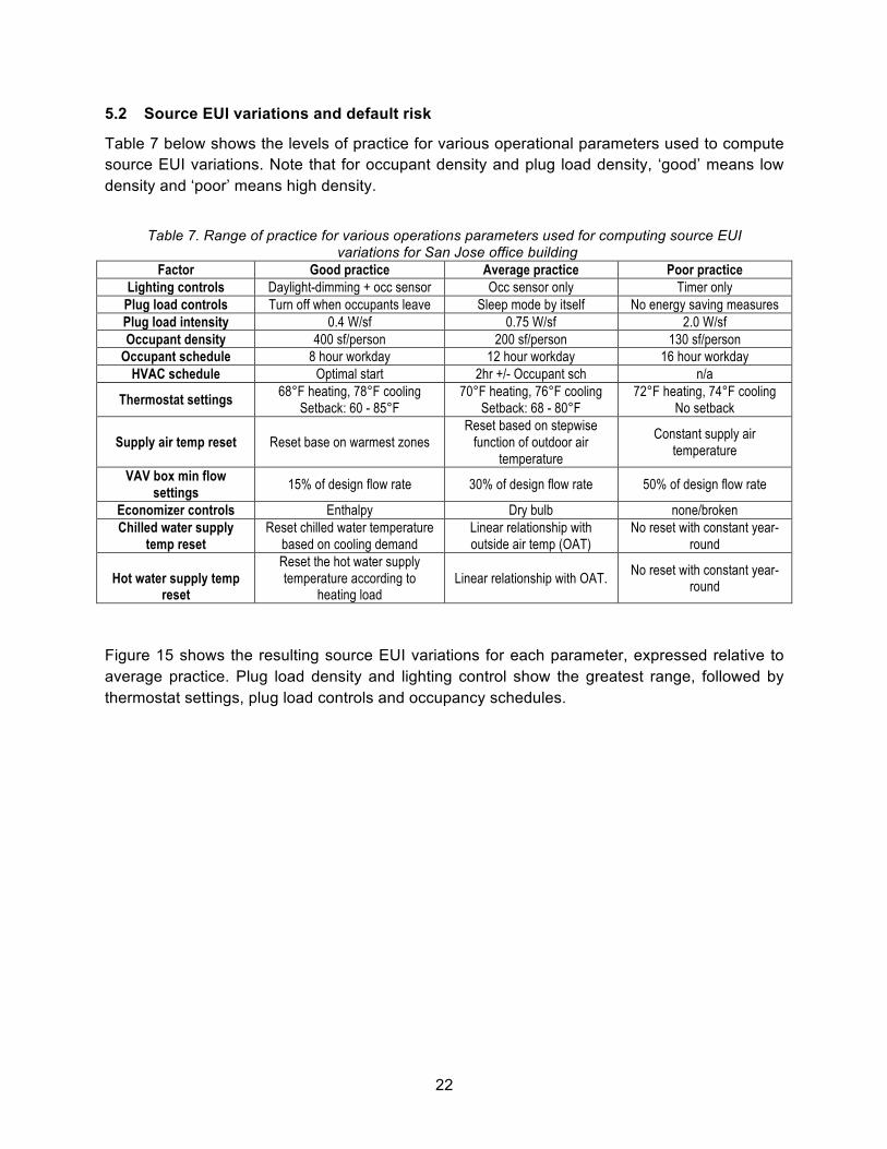
5.2 Source EUI variations and default risk
Table 7 below shows the levels of practice for various operational parameters used to compute source EUI variations. Note that for occupant density and plug load density, ‘good’ means low density and ‘poor’ means high density.
Table 7. Range of practice for various operations parameters used for computing source EUI variations for San Jose office building
Factor Good practice Average practice Poor practice Lighting controls Daylight-dimming + occ sensor Occ sensor only Timer only
Plug load controls Turn off when occupants leave Sleep mode by itself No energy saving measures Plug load intensity 0.4 W/sf 0.75 W/sf 2.0 W/sf Occupant density 400 sf/person 200 sf/person 130 sf/person
Occupant schedule 8 hour workday 12 hour workday 16 hour workday HVAC schedule Optimal start 2hr +/- Occupant sch n/a
Thermostat settings 68°F heating, 78°F cooling Setback: 60 - 85°F
70°F heating, 76°F cooling Setback: 68 - 80°F
72°F heating, 74°F cooling No setback
Supply air temp reset Reset base on warmest zones Reset based on stepwise
function of outdoor air temperature
Constant supply air temperature
VAV box min flow settings 15% of design flow rate 30% of design flow rate 50% of design flow rate
Economizer controls Enthalpy Dry bulb none/broken Chilled water supply
temp reset Reset chilled water temperature
based on cooling demand Linear relationship with outside air temp (OAT)
No reset with constant year-round
Hot water supply temp reset
Reset the hot water supply temperature according to
heating load Linear relationship with OAT. No reset with constant year-
round
Figure 15 shows the resulting source EUI variations for each parameter, expressed relative to average practice. Plug load density and lighting control show the greatest range, followed by thermostat settings, plug load controls and occupancy schedules.

23
Figure 15. Simulated relative source EUI variations due to poor and good operational
practices for San Jose office building. Values are relative to average practice.
We then computed the source EUI variations for scenarios that represented various combinations of practice levels. The parameters were grouped into two categories:
● Facilities management (FM) parameters are those largely controlled by the building facilities management staff. These include HVAC schedule, thermostat settings, supply air temperature reset, VAV minimum flow settings, economizer controls, chilled and hot water temperature reset, and lighting controls.
● Occupancy practices (OP) are largely a function of occupant behavior and business function, with little or no facilities influence. These include occupant density, occupant schedule, plug load density, and plug load controls.
Finally, we calculated how these source EUI variations translate into variations in default rate, based on the default rate logistic regression model coefficients, as described earlier. Table 8 and Figure 16 show the results, again expressed as variation relative to average practice. Good practice across all parameters yields 40% lower source EUI and 161 basis points (bp) reduction in default rate compared to the average case. Poor practice across all parameters yields 183% higher source EUI and 331 bp increase in default rate relative to average practice. Good practice facilities management alone, with average occupant practice, yields an 18% reduction in source EUI and 63 bp reduction in default rate.
-30
-20
-10
0
10
20
30
40
50
Ligh-n
gCtrl
Plugload
Ctrl
Plugload
Density
OccDe
nsity
OccSch
HVAC
sch
ThermoSet
SAT
VAVm
in
Econ
omizer
ChWaterTempR
eset
HotW
aterTempR
eset
Ligh-ng Plugload Occupant HVAC
(%)
SanJoseOffice-Rela-veChangeinSourceEUI
Goodprac-ce Poorprac-ce
24
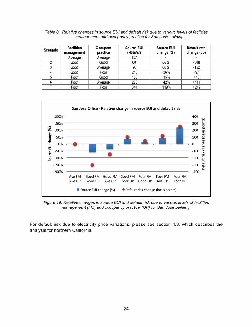
Table 8. Relative changes in source EUI and default risk due to various levels of facilities management and occupancy practice for San Jose building.
Scenario Facilities management
Occupant practice
Source EUI (kBtu/sf)
Source EUI change (%)
Default rate change (bp)
1 Average Average 157 - - 2 Good Good 60 -62% -308 3 Good Average 98 -38% -152 4 Good Poor 213 +36% +97 5 Poor Good 180 +15% +43 6 Poor Average 223 +42% +111 7 Poor Poor 344 +119% +249
Figure 16. Relative changes in source EUI and default risk due to various levels of facilities
management (FM) and occupancy practice (OP) for San Jose building. For default risk due to electricity price variations, please see section 4.3, which describes the analysis for northern California.
-400
-300
-200
-100
0
100
200
300
400
-200%
-150%
-100%
-50%
0%
50%
100%
150%
200%
AveFMAveOP
GoodFMGoodOP
GoodFMAveOP
GoodFMPoorOP
PoorFMGoodOP
PoorFMAveOP
PoorFMPoorOP
Defaultriskchan
ge(b
asispoints)
SourceEUIcha
nge(%
)
SanJoseOffice-Rela@vechangeinsourceEUIanddefaultrisk
SourceEUIchange(%) Defaultriskchange(basispoints)

25
6 Denver Hotel
6.1 Energy model overview
This limited service hotel, located in the Denver metropolitan area, has 157 guest rooms with a gross floor area of 89,000 sf. Facilities include a breakfast area, kitchen, fitness center, indoor pool and laundry facilities. It was constructed in 1997. Figure 17 shows the simulation model geometry for the building. The current mortgage loan was funded in 2014. The loan documents included floor plans, photographs, and a room schedule. We used this information along with Google Earth to determine overall geometry, thermal zoning, window locations and size. The loan documents also had some information on the building envelope and HVAC systems. The walls are wood frame with a combination of stucco and exposed brick. The roof is a plywood deck with concrete tile shingles. The windows are double pane with vinyl frames. The guest rooms have through-the-wall packaged terminal air conditioner (PTAC) units. The common areas are heated and cooled with packaged rooftop units. We assumed lighting and HVAC efficiency from ASHRAE 90.1-1989. For building operational characteristics such as plug load density and schedules, we assumed values from the DOE reference model for small hotels post-1980.
Figure 17. Simulation model geometry of Denver hotel building.
The total source energy (electricity and natural gas) for the baseline model was 16,084 MMBtu, with a source EUI of 180 kBtu/sf. Figure 18 shows the energy use breakout from the baseline simulation model.

26
Figure 18. Simulated source energy end uses for Denver hotel building.
The appraisal report did not include any historical energy use information. As a reasonableness check, we compared the source EUI to a peer group from the DOE Building Performance Database. The peer group was comprised of 15 hotels in climate zone 5C (cool dry) that are less than 100,000 sf (this eliminates larger full-service hotels). Figure 19 shows the distribution of source EUI for this peer group. The median value is 154 kBtu/sf, with a 25-75 percentile range of 111-189 kBtu/sf. This shows that the simulated EUI is within the range of reasonableness.
Figure 19. Screen image from the DOE Building Performance Database (BPD) showing
measured source EUI distribution for a peer group of 15 hotels in climate zone 5B (cool-dry), less than 100,000 sf. Grey balloon shows source EUI for simulated building.
HVAC34%
Ligh-ng25%
Equipment35%
DHW6%
DenverHotelSourceEnergyEndUses

27
6.2 Source EUI variations and default risk
Table 9 below shows the levels of practice for various operational parameters used to compute source EUI variations. Energy use in guest rooms also varies by vacancy level. We modeled three vacancy levels: average of 35% based on the DOE reference model; high of 50%, and low of 10% (note that for vacancy levels, “good” means higher vacancy and “poor” means lower, consistent with their impact on energy usage only). We would also note that this list of parameters is rather limited and does not include common area parameters such as kitchen and laundry equipment efficiency and controls. We did not have readily available information on different levels of practice for such parameters and it was beyond the scope of this study to investigate them.
Table 9. Range of practice for various operations parameters used for computing source EUI variations for Denver hotel building
Factor Good practice Average practice Poor practice Common area lighting
controls Daylight-dimming + occ sensor Occ sensor only Timer only
Common area thermostat settings
68°F heating, 78°F cooling Setback: 60 - 85°F
70°F heating, 76°F cooling Setback: 68 - 80°F
72°F heating, 74°F cooling No setback
Common area economizer controls Enthalpy Dry bulb none/broken
DHW temperature setting 120°F 140°F not modeled
Guest room vacancy5 controls HVAC off, lights off HVAC setback, lights off No HVAC setback, lights on
Guest room vacancy level 50% 35% 10%
Figure 20 shows the resulting source EUI variations for each parameter, expressed relative to average practice. As expected, guest room vacancy dwarfs the impact of common area parameters. Given the limited scope of the parameters considered, the source EUI variations are conservative – i.e., smaller than they would be if a broader set of parameters were considered.
5 Note that vacancy in this case indicates when guest rooms are not rented out. It does not refer to controls when the rooms are rented but unoccupied.

28
Figure 20. Simulated relative source EUI variations due to poor and good operational
practices for Denver hotel building. Values are relative to average practice.
We then computed the source EUI variations for scenarios that represented various combinations of parameters. The parameters were grouped into three categories:
● Guest room vacancy level i.e. percentage of guest rooms that are vacant. ● Guest room vacancy controls refer to how guest room HVAC and lighting is controlled in
vacant guest rooms. ● Common area parameters include common area thermostat settings, economizer
controls, lighting controls and domestic hot water settings. Finally, we calculated how these source EUI variations translate into variations in default rate, based on the default rate logistic regression model coefficients, as described earlier. Table 10 and Figure 21 show the results, again expressed as variation relative to average practice. Good practice across all parameters with 35% vacancy level yields 7% lower source EUI and 23 basis points (bp) reduction in default rate compared to the average case. Poor practice across all parameters with 35% vacancy yields 17% higher source EUI and 49 bp increase in default rate relative to average practice. Assuming average practice in all parameters, just a change in vacancy level from 35% to 10% yields a 7% increase in source EUI. Similarly, 50% vacancy results in 5% reduction in source EUI. With a vacancy level of 50%, good to poor practice guest room controls shows a range of -11% to +12% in source EUI and -37 to +36 bp for default rate.
-10
-5
0
5
10
15
20
Ligh+n
gCtrl
ThermoSet
Econ
omizer
DHWtemp
Vacancy35
Vacancy10
Vacancy50
AllCom
bine
d-35
Ligh+ng HVAC DHW VacancyLevel
(%)
DenverHotel-Rela+veChangeinSourceEUI
Goodprac+ce Poorprac+ce

29
Table 10. Relative changes in Source EUI and default risk due to various levels of facilities management and occupancy practice for Denver hotel building.
Scenario Guest room
vacancy level Guest room
controls Common area
practice Source EUI
(kBtu/sf) Source EUI change (%)
Default rate change (bp)
1 35% Average Average 180 - - 2 35% Good Average 173 -4% -12 3 35% Poor Average 201 +12% +36 4 35% Good Good 167 -7% -23 5 35% Poor Poor 210 +17% +49 6 10% Good Average 193 +7% +22 7 10% Average Average 194 +8% +24 8 10% Poor Average 201 +12% +35 9 50% Good Average 160 -11% -37
10 50% Average Average 171 -5% -17 11 50% Poor Average 202 +12% +36
Figure 21. Relative changes in source EUI and default risk due to various levels of vacancy
(Vac), guest room controls (GC), and common area (CA) practice for Denver hotel. For default risk due to electricity price variations, please see section 3.3, which describes the analysis for the Denver area.
-80
-60
-40
-20
0
20
40
60
80
-20%
-15%
-10%
-5%
0%
5%
10%
15%
20%
35%VacAveGCAveCA
35%VacGoodGCAveCA
35%VacPoorGCAveCA
35%VacGoodGCGoodCA
35%VacPoorGCPoorCA
10%VacAveGCAveCA
10%VacGoodGCAveCA
10%VacPoorGCAveCA
50%VacAveGCAveCA
50%VacGoodGCAveCA
50%VacPoorGCAveCA
Defaultriskchan
ge(b
asispoints)
SourceEUIcha
nge(%
)
Rela<vechangeinsourceEUIanddefaultriskforvariousscenarios
SourceEUIchange(%) Defaultriskchange(basispoints)

30
7 San Francisco Multi-family Building
7.1 Energy model overview
This eight-story multi-family building located in San Francisco has 75 residential units with a gross floor area of 94,000 sf, including a small amount of retail space at about 2,000 sf net area. Construction was completed in 2014. Figure 22 shows the simulation model geometry for the building. The loan documents included floor plans, photographs, and a list of unit types. We used this information along with Google Earth to determine overall geometry, thermal zoning, window locations and size. The loan documents also had some information on the building envelope and HVAC systems. The walls are wood frame with cement plaster. The roof is a built-up composition roof. The residential units do not have any air conditioning. The residential units and common areas have baseboard radiators fed by a gas-fired hot water boiler. The retail area has an air-source heat pump. A rooftop gas-fired packaged heating and ventilation unit provides complementary air to the corridors. There is a solar thermal domestic hot water pre-heating system on the roof. We assumed lighting and HVAC efficiency from California Title 24-2013 energy code. Building operational characteristics such as residential occupancy schedules were also assumed from Title 24.
Figure 22. Simulation model geometry of San Francisco multi-family building.
The total source energy (electricity and natural gas) for the baseline model was 5,135 MMBtu, with a source EUI of 54 kBtu/sf. Figure 23 shows the energy use breakout from the baseline simulation model.

31
Figure 23. Simulated source energy end uses for San Francisco multi-family building.
The appraisal report did not include any historical energy use information. As a reasonableness check, we compared the source EUI to a peer group from the DOE Building Performance Database. The peer group was comprised of 30 multi-family buildings in San Francisco ranging in size from 30,000-120,000 sf (the lower bound eliminates smaller multi-family units). Figure 24 shows the distribution of source EUI for this peer group. The median value is 58 kBtu/sf, with a 25-75 percentile range of 34-102 kBtu/sf. This shows that the simulated EUI is very close to the median value, and within the range of reasonableness.
Figure 24. Screen image from the DOE Building Performance Database (BPD) showing
measured source EUI distribution for a peer group of 30 multi-family buildings in San Francisco ranging from 30,000-120,000 sf. Grey balloon shows source EUI for simulated
building.
HVAC9%
Ligh,ng30%
Plugloads40%
DHW21%
SanFranciscoMul,-familySourceEnergyEndUses
32
7.2 Source EUI variations and default risk
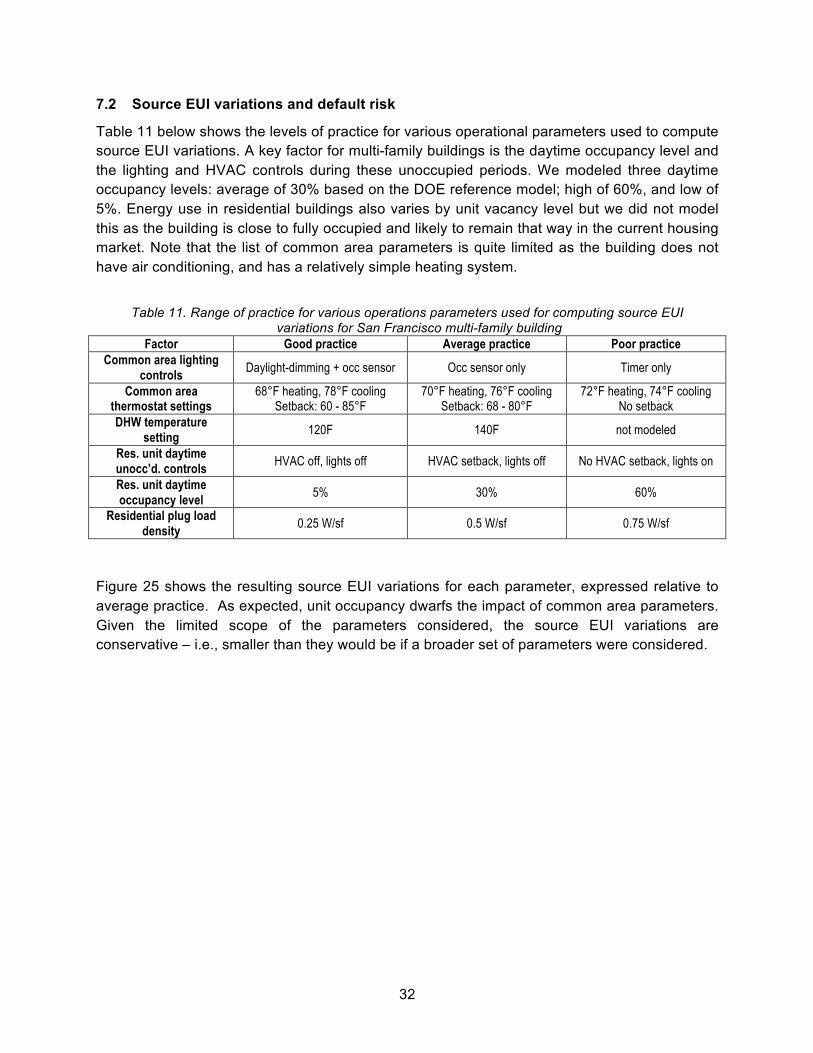
Table 11 below shows the levels of practice for various operational parameters used to compute source EUI variations. A key factor for multi-family buildings is the daytime occupancy level and the lighting and HVAC controls during these unoccupied periods. We modeled three daytime occupancy levels: average of 30% based on the DOE reference model; high of 60%, and low of 5%. Energy use in residential buildings also varies by unit vacancy level but we did not model this as the building is close to fully occupied and likely to remain that way in the current housing market. Note that the list of common area parameters is quite limited as the building does not have air conditioning, and has a relatively simple heating system.
Table 11. Range of practice for various operations parameters used for computing source EUI variations for San Francisco multi-family building
Factor Good practice Average practice Poor practice Common area lighting
controls Daylight-dimming + occ sensor Occ sensor only Timer only
Common area thermostat settings
68°F heating, 78°F cooling Setback: 60 - 85°F
70°F heating, 76°F cooling Setback: 68 - 80°F
72°F heating, 74°F cooling No setback
DHW temperature setting 120F 140F not modeled
Res. unit daytime unocc’d. controls HVAC off, lights off HVAC setback, lights off No HVAC setback, lights on
Res. unit daytime occupancy level 5% 30% 60%
Residential plug load density 0.25 W/sf 0.5 W/sf 0.75 W/sf
Figure 25 shows the resulting source EUI variations for each parameter, expressed relative to average practice. As expected, unit occupancy dwarfs the impact of common area parameters. Given the limited scope of the parameters considered, the source EUI variations are conservative – i.e., smaller than they would be if a broader set of parameters were considered.

33
Figure 25. Simulated relative source EUI variations due to poor and good operational
practices for San Francisco multi-family building. Values are relative to average practice.
We then computed the source EUI variations for scenarios that represented various combinations of parameters. The parameters were grouped into three categories:
● Residential daytime occupancy level – i.e., percentage of units that are occupied during the day.
● Residential operations practice (RO) – i.e. how HVAC and lighting is controlled during unoccupied periods.
● Plug load intensity (PL) in residential units. In this context, ”good” refers to low intensity and ”poor” refers to high intensity.
● Facilities management (FM) parameters include common area lighting controls, thermostat settings, and domestic hot water settings.
Finally, we calculated how these source EUI variations translate into variations in default rate, based on the default rate logistic regression model coefficients as described earlier. Table 12 and Figure 26 show the results, again expressed as variation relative to average practice and average daytime occupancy. Good practice across all parameters with average daytime occupancy level yields a 20% lower source EUI and 72 basis point (bp) reduction in default rate compared to the average practice case. Poor practice across all parameters with average daytime occupancy level yields a 26% higher source EUI and 74 bp increase in default rate relative to average practice. As expected the relative changes in source EUI and default risk are more pronounced with lower daytime occupancy levels.
0
-30
-20
-10
0
10
20
30
Ligh+ngCtrl
ThermoSet
DHWtemp
Plugload
Occ30%
Occ60%
Occ5%
Combine
d-Occ30%
CommonArea DHW ResPlugload ResDayOccLevel
(%)
SanFranciscoMul+-family-Rela+veChangeinSourceEUI
Goodprac+ce Poorprac+ce

34
Table 12. Relative changes in source EUI and default rate due to various levels of facilities management and occupancy practice for San Francisco multi-family building.
Scenario Res day
occ level Res ops practice
Res plug load
Fac. mgmt. practice
Source EUI (kBtu/sf)
Source EUI change (%)
Default rate change (bp)
1 30% Average Average Average 56 - 2 30% Good Low Good 45 -20.3% -72 3 30% Average Average Good 49 -11.9% -40 4 30% Good Low Poor 55 -2.2% -7 5 30% Average Average Poor 60 6.9% 21 6 30% Poor High Good 60 7.2% 22 7 30% Poor High Poor 71 26.3% 74 8 60% Average Average Average 57 1.6% 5 9 60% Good Average Average 56 0.6% 2
10 60% Poor Average Average 60 7.4% 23 11 5% Average Average Average 52 -7.1% -23 12 5% Good Average Average 51 -8.4% -28 13 5% Poor Average Average 61 8.5% 26
Figure 26. Relative changes in source EUI and default risk due to various levels of daytime occupancy (DO), resident operations practice (RO), resident plug load intensity (PL) and
facilities management (PM) practice for San Francisco multi-family building. For default risk due to electricity price variations, please see section 3.3, which describes the analysis for northern California.
-80
-60
-40
-20
0
20
40
60
80
-30%
-20%
-10%
0%
10%
20%
30%
30%OccAveROAvePLAveFM
30%OccGoodROLowPLGoodFM
30%OccAveROAvePL
GoodFM
30%OccGoodROLowPLPoorFM
30%OccAveROAvePLPoorFM
30%OccPoorROHighPLGoodFM
30%OccPoorROHighPLPoorFM
60%OccAveROAvePLAveFM
60%OccGoodROAvePLAveFM
60%VacPoorROAvePLAveFM
5%OccAveROAvePLAveFM
5%OccGoodROAvePLAveFM
5%OccPoorROAvePLAveFM
Defaultriskchan
ge(b
asispoints)
SourceEUIcha
nge(%
)
SanFranciscoMul=-family-Rela=vechangeinsourceEUIanddefaultrisk
SourceEUIchange(%) Defaultriskchange(basispoints)

35
8 Conclusions and Recommendations This report documents the impact of energy use and price variations on commercial mortgage default risk in five buildings: an office building and hotel in the Denver area, two office buildings in northern California, and a multi-family residential building in San Francisco. We used parametric energy simulation to analyze the impact of variations in operational practices on source energy use intensity. We also modeled various combinations of poor, average, and good practice in each parameter. We then computed the impact of source EUI variations on default risk using coefficients from an empirical logistic regression model developed earlier in this research effort as documented in Wallace et al. [2017]. Table 13 shows the relative range of variation in source EUI and default risk for each building. The table also shows the default rate variation relative to the TREPP average default rate of 800bp.
Table 13. Range of variation in source EUI and default risk for five case studies.
Building Source EUI variation (%) Default rate variation (bp)
Default rate variation relative to 8% avg. (TREPP)
Denver Office -54% to +132% -248 to +268 -31% to +34% Sonoma Office -40% to +183% -161 to +331 -20% to +41% San Jose Office -62% to +119% -308 to +249 -39% to +31% Denver Hotel -11% to +17% -37 to +49 -5% to +6% San Francisco Multi-family -20% to +26% -72 to +74 -9% to +9%
To summarize, we found that variations in energy use that are reasonably common could raise or lower the default rates in these properties by between roughly 5% and 40%, depending on the property type and geography. This is a fairly significant potential impact, especially given our prior finding that the industry generally does not take energy usage into consideration in assessing loans [Mathew et al., 2016] We computed the impact of electricity price variations in the Denver area and northern California using variations of wholesale electricity prices. Table 14 shows the relative range of variation in default risk corresponding to one standard deviation variation in electricity price gap.
Table 14. Range of variation in electricity price gap and default risk for the Denver area and northern California.
Wholesale price region Default rate variation (bp)
Default rate variation relative to TREPP avg (%)
Denver area +159 to +501 +20% to +63% Northern California -49 to +705 -6% to +88%
It is important to note the limitations of this study:
• The source EUI variations are based on a limited number of parameters. In that sense, they are somewhat conservative and the actual range for these buildings could be higher. This is especially true for the Denver hotel.
• The default rate calculations assume that the default rate coefficients from the logistic regression model are generally applicable to each of these buildings individually.
• The electricity price gap variations are based on wholesale electricity price, and not the specific retail rate for these buildings.
• The study does not distinguish between net and gross leasing structures.

36
Given the above, these results should be seen as indicative of the default risks, rather than precise estimates of default rate for a given building. We presented and discussed these findings with each of the three lender organizations that provided the data for these case studies. All three lenders indicated that these findings are meaningful and that the range of default risk variations are material. As one lender stated: “these results showing the impact of energy on default risk are clearly meaningful. I don't currently consider energy efficiency when making a loan and seeing this makes me think I would want to ask about it.” We also discussed potential approaches to effectively incorporate energy costs and risks into the underwriting process. There are well established methods to analyze energy use, costs, and risks. These include audits, benchmarking, utility bill analysis, etc. There are even standards for some of these activities. ASHRAE has guidelines for three levels of energy audits [ASHRAE 2011]. ASTM 2797-15 establishes a standard specifically for assessing energy performance in the context of a real estate transaction, and includes analysis of variation [ASTM 2015]. However, a key market limitation is that most lender organizations do not have the interest or expertise to use such detailed information. Furthermore, there continue to be pressures to limit the cost and time for engineering analyses. These lenders suggested that a more viable approach is to have a simple risk ratio or score that they can use during underwriting. For example, seismic and other natural hazard risks are currently captured in a simple numeric score with thresholds. If the building exceeds the threshold risk, the lender can either reject the loan or require mitigating measures. Based on these discussions with lenders and other stakeholders, we recommend the following in the near term:
• Lenders should request an estimate of energy cost variations as part of the loan application. This may be based on historical utility bill data or more in-depth analysis if that is available. This will at a minimum provide lenders a range of variation that they can factor into the NOI analysis. More broadly from a market transformation standpoint, it will signal to owners that energy costs matter to the lender.
• Develop a simple-to-use energy risk score that can be used for underwriting, analogous to the seismic risk score. Notably, the lenders indicated that they would be willing to pilot such a score on new loans.

37
9 References ASHRAE 2011. Procedures For Commercial Building Energy Audits. Second Edition. American Society for Heating Refrigerating and Air conditioning Engineers. Atlanta, Georgia. https://www.ashrae.org/resources--publications/bookstore/procedures-for-commercial-building-energy-audits. Accessed April 2016. ASTM 2797-15. Standard Practice for Building Energy Performance Assessment for a Building Involved in a Real Estate Transaction. http://www.astm.org/Standards/E2797.htm. Accessed April 2016. Mathew, P., Coleman, P., Wallace, N., Issler, P., Kolstad, L., Sahadi, R. Energy Factors in Commercial Mortgages: Gaps and Opportunities. Technical Report. Lawrence Berkeley National Laboratory. May 2016. LBNL-1006378 Wallace, N., Issler, P., Mathew, P., Sun, K. Impact of Energy Factors on Default Risk in Commercial Mortgages. Technical Report. Lawrence Berkeley National Laboratory. 2017. https://cbs.lbl.gov/energy-factors-commercial-mortgages. Accessed September 2017.