morphology development in kenics static mixers

604 The Canadian Journal of Chemical Engineering, Volume 80, August 2002

Systematic studies of mixing processes have received a considerableamount of attention, because of their importance both in natureand in industry. Although in many cases mixing is associated with

turbulent fluid motions, mixing of very viscous fluids constitutes anotherimportant class of mixing occurrences, and is typical for polymerblending, compounding, food processing, etc. Analysis of laminarmixing behavior in three-dimensional flows started with the paper ofFeingold et al. (1988), and was followed by numerical studies, includingthose of Bajer and Mofatt (1990), Ashwin and King (1995), Anderson etal. (1999), and Fountain et al. (2000), studying all types of interestingphenomena occurring in three-dimensional flows. Experimental workhas focused on chaotic mixing in three-dimensional flows in pipes(Peerhossaini et al., 1993), and major advances in the area of visualizationof these three-dimensional flows are achieved by the work of Kusch andOttino (1992) who studied chaotic advection in some continuous flows.Khakhar et al. (1987) analyzed one of these systems in more detail, thepartitioned pipe mixer (PPM), consisting of a pipe and series of flatpartitions at right angles to each other. These experimental studiesclearly show regular and chaotic mixing in a three-dimensional flow.

The traditional solution to many mixing problems has been toincrease the energy input to the process, and to let the turbulence of thevelocity field produce effective mixing. With the high viscosities associatedwith (bio-) polymers, turbulent flow is not achievable and laminar flow isthe only possible mechanism for polymer mixing. As already observed byReynolds (1894) more than 100 years ago, effective (laminar) mixing offluids arises due to repeated stretching and folding. Typical mixers aredesigned such that material is efficiently stretched and folded as in thefamous bakers transformation, providing a direct connection betweenchaos and fluid mixing (Aref, 1984). The quality of mixing, characterizedby the increase of interfacial area, the number of folds or striations, orthe reciprocal of the striation thickness, may increase exponentially. Also,for these laminar flows it is well-known that an increase of energyapplied to the system does not have to lead to better mixing.

Characteristics of chaotic periodic mixing flows are determined by thelocation and nature of the periodic points (Ottino, 1989). Such aperiodic point analysis is a powerful tool to study details of periodicflows, especially when higher-order periodic points are included in theanalysis. A disadvantage of such an elegant, but computationallyexpensive analysis, is that all the work has to be repeated if one modifies

*Author to whom correspondence may be addressed. E-mail address:[email protected]

Morphology Development in Kenics Static Mixers(Application of the Extended Mapping Method)

Oleksiy S. Galaktionov, Patrick D. Anderson*, Gerrit W.M. Peters and Han E.H. Meijer

Dutch Polymer Institute, Materials Technology, Eindhoven University of Technology, P.O. Box 513, 5600 MBEindhoven, The Netherlands

This paper addresses the interfacial area generationin Kenics static mixers using a new method. A statisticaldescription of the microstructure development isobtained using the extended mapping method, whichis restricted to systems with negligible interfacialtension. However, the layered structures created in aKenics are a good example where interfacial tensiondoes not play an important role (the layered structureis retained). The extended mapping method isadopted to the special flow conditions in spatiallyperiodic flows. The efficiency of the interface generationfor different mixer layouts is compared and additionalattention is given to the distribution of the interfacialarea across the mixer. It is shown that the extendedmapping method enables us to find the bladeconfiguration that optimizes the mixing performance,in accordance to the standard mapping method, butnow including much more details concerning themicrostructure development in this chaotic flow.

On examine dans cet article la formation de lasurface interfaciale dans les mélangeurs statiques Kenicsà l’aide d’une nouvelle méthode. Une descriptionstatistique du développement de la microstructure estobtenue par la méthode de projection étendue, quiest réservée aux systèmes ayant une tension interfacialenégligeable. Toutefois, les structures stratifiées crééesdans un Kenics sont un bon exemple où la tensioninterfaciale ne joue pas un rôle important (la structureen couche est retenue). La méthode de projectionétendue est adaptée aux conditions d’écoulementspériodiques sur le plan spatial. L’efficacité de laformation de l’interface pour différentes configurationsde mélangeurs est comparée et une attention particulièreest portée à la distribution de la surface interfacialedans le mélangeur. On montre que la méthode deprojection étendue permet de trouver la configurationdes lames donnant une performance de mélangeoptimale, en accord avec la méthode de projectionstandard, mais on fournit beaucoup plus d’informationssur le développement de la microstructure dans cetécoulement chaotique.

Keywords: laminar mixing, Kenics static mixer,microstructure, mapping method.


the flow protocol. In the line of the original concepts of Spencer andWiley (1951), a somewhat different approach to study periodicmixing flows has been suggested by Galaktionov et al. (2001)and Kruijt et al. (2001a). This technique, called the mappingmethod, does not provide all details about mixing characteristicslike periodic points or Poincare sections, but does offer a flexibleand elegant way to study a wide range of mixing occurrenceswith only little computational power. Examples of the mappingmethod applications can be found in Kruijt et al. (2001b, c).

This paper deals with morphology development in Kenicsstatic mixers, and an extension of the mapping technique forstatic mixers is developed to include a description for themicrostructure in the flow. The extended mapping technique,which utilizes a special area tensor to describe the microstruc-ture in a statistical way, was developed and applied to two-dimensional time-periodic mixing flows (Galaktionov et al.,2002a; Anderson et al., 2002), where it proved to be a usefultool for modeling microstructure development. Someimportant aspects of laminar mixing, such as self-similarity ofthe interface patterns, exponential-in-time stretching of thematerial and asymptotic directionality were properly captured.In this paper we will describe the adaptation of the extendedmapping technique to spatially periodic flows. This techniquewill then be applied to Kenics static mixers. The efficiency of theKenics mixers of different configuration in interfacial area genera-tion will be compared. Finally, the irregularity of the volumetricinterfacial area density distribution across the mixers will beaddressed.

Methods and Formulation Mixer Geometry and Velocity Field The Kenics static mixer consists of a cylindrical pipe with mixingelements fixed inside (see Figure 1a). The mixing elements arehelically twisted rigid plates (usually with the same pitch), eachdividing the pipe into two twisted semicircular ducts. The inserts areplaced tightly one after another so that the leading edge of the nextinsert is perpendicular to the trailing edge of the previous one. Theflow along the pipe is caused by the imposed pressure difference.

The velocity field inside Kenics mixers was obtained in previouswork (Galaktionov et al., 2002b). The computational flow domainused in Galaktionov et al. (2002b) is shown in Figure 1b. It providesall basic elements needed to construct various mixer configurations:long (twisted by 180°) blade and transition zones between similarlyand oppositely twisted blades. The finite element mesh used tocompute the velocity field is illustrated by Figure 1c. The meshcontained 13824 second-order hexagonal elements with 116145nodal points (403 731 degrees of freedom). It was found that theflow in the mixer channels can be safely regarded as undisturbed ata 45° blade twist away from the blade transition zones. The straightin-flow and out-flow sections of the domain make it possible toprescribe a fully developed Poiseuille velocity profile as a boundarycondition. The axial velocity through the straight semi-circular ductcan be expressed by an analytical function (Meleshko et al., 1999).

Through the paper we refer to the mixers with the bladestwisted in alternating directions as ‘RL’ configurations, and tomixers with all blades twisted in the same direction as ‘RR’configurations. The number, like in the notation ‘RL-180’(Figure 1a) denotes the blade twist angle, measured in degrees.

Figure 1. a) The schematic view of the ‘standard’ Kenics mixer (RL-180). b) The computational domain, providing all necessary features. c) Finiteelement mesh, covering the computational domain (fitted to blade geometry). d) Computing the mapping matrix and interface deformation:tracing the flow tube between two cross-sections.

Mapping Results The basic idea of the mapping method is to construct a mapping fora mixing-related quantity, like concentration of fluid or interfacialarea, from a well-defined initial reference grid to a deformed grid.The mapping can be easily defined using a matrix with coefficientscontaining for each cell of the deformed grid the fraction of thiscell in the original grid. If our mixing-related quantity is a scalarquantity, like the concentration vector C defined on our grid,which is additive, then it follows that the concentration C1 after thedeformation, can be obtained by multiplying the initial concentrationvector C0 with the mapping matrix F:

C1 = FC0 (1)

For time-periodic mixing flows the original and deformedgrid are referenced using time; for spatial-periodic mixing flowsthey are referenced using an appropriate, to be chosen, spatialparameter. In both cases the deformed grid is obtained bytracking the original grid to the reference level, either in time(dt) or space (dz). One of the main advantages of this techniqueis that once the matrix � is computed, we can simply computethe deformation of the initial concentration vector C0 after ntimes dt or dz by simply repeating the matrix-vector multiplication:

Note that the matrix-vector multiplications are repeated n timesinstead of computing the Fn. More details on the implementationof the mapping method can be found in Galaktionov et al. (2001).

Figure 1d contains a representation of a part of the Kenicsstatic mixer. In the bottom of this plot a coarse initial two-dimensional reference grid is shown and the displacement ofone cell during flow is plotted. The intersections of thisdeformed cell with the original cells (in the exit plane)determine one column of the mapping matrix. The entries ofthe remaining columns are determined in a similar way by

(2)C Cn

n

= ( )ÈÎÍ

˘˚

ÏÌÓ¸˛

F F FK K1 2444 3444

0

times

tracking all other cells and determining their intersections withthe original grid. The actual grids used in the computationscontain 1.6 ¥ 105 cells (400 ¥ 400 resolution). The issues of theconvergence of the extended mapping technique were studiedin Anderson et al. (2002) using a prototype mixing flow. In thecurrent paper the 400 ¥ 400 mapping grids are used to ensure asuitable graphic quality. The Kenics mixer in general is intendedto mimic to a possible extent the ‘bakers transformation’ (see,for example Ottino, (1989): repetitive stretching, cutting andstacking. To illustrate the principles of the Kenics static mixer aseries of the concentration profiles inside the first elements ofthe ‘standard’ mixer with blades twisted by 180° in alternatingdirections (referred to as RL-180) is presented in Figure 2. Thefirst image shows the initial pattern at the beginning of the firstelement: each channel is filled partly by black (c = 1) and partlyby white (c = 0) fluid, with the interface perpendicular to the blade.The total influx of both fluid components is equal.

The images in Figure 2b to 2e show the evolution of theconcentration distribution along the first blade; the thindashed line in Figure 2e denotes the leading edge of the next blade.From the point of view of mimicking the bakers transformation itseems that the RL-180 mixer has too large a blade twist:the created layers do not have even roughly equal thickness. Theconfiguration achieved 1/4 blade earlier (see Figure 2d) looks muchmore preferable. The next frame, Figure 2f, shows the mixturepatterns just 10° into the second, oppositely twisted, blade. Thestriations, created by the preceding blade are cut and dislocatedat the blade. As a result, at the end of the second blade (Figure2g) the number of striations is doubled. After four mixingelements, Figure 2h, sixteen striations are found in eachchannel. The Kenics mixer roughly doubles the number ofstriations with each blade, although some striations may notstretch across the whole channel width. Notice that the imagesin Figure 2 show the actual spatial orientation of the striationsand mixer blades. In all other figures in the rest of this paper thepatterns are transformed to the same orientation: the blade —its trailing edge — is positioned horizontally. This simplifies thecomparison of self-similar distributions.

The Canadian Journal of Chemical Engineering, Volume 80, August 2002 606

Figure 2. How the Kenics mixer works: the frames show the evolution of concentration patterns within the first four blades of the RL-180 mixer.

The Extended Mapping Approach forSpatially Periodic Flows To study microstructure development during mixing, theextended mapping technique, which makes use of the areatensor, was implemented for two-dimensional time-periodicprototype mixing flows (Galaktionov et al., 2002a; Andersonet al., 2002). However, the application of the mappingtechnique to static mixers, which are spatially periodic, is newand has some special features that are discussed first.

Here, steady Stokes flow in the Kenics mixer is consideredand, as a result, the pattern of intermaterial interfaces does notchange in time. Consequently, the velocity vectors at theinterface are always parallel to the interface. Moreover, inthe considered system the axial velocities are always positive inthe core of the flow and only equal to zero at rigid boundaries.If in a lateral cross-section of the mixer, the location of theinterfaces is known together with the three-dimensionalvelocity field, the interface configuration is fully defined and canbe restored by merely tracking the contours along the flow.

The interface configuration at the initial cross-section shouldbe specified explicitly by giving the interface contours shape.Tracking, which is performed using the z coordinate as anindependent variable, establishes a one-to-one correspondencebetween all points of the initial and the final plane. We can considerthis relation as a two-dimensional transformation (or “map” in themathematical sense of the word). This transformation away fromthe blade transitions is continuous but not area preserving.However, the flux is being conserved.

The interfacial contours in the mixer cross-section aredescribed using the two-dimensional area tensor. For the two-dimensional transformation that establishes relations betweenthe initial and final cross-section, a pseudo deformation gradienttensor is defined. In two-dimensional flows, considered inAnderson et al. (2002) and Galaktionov et al. (2002a), thedeformation gradient tensor was used to transform the area

tensor according to local deformation patterns. The techniqueinvolved the finding of a unique droplet shape tensor,transforming it with deformation gradient tensor andtransforming the result back into a corresponding area tensor.The pseudo deformation tensor is defined as follows. Considera material point p, going from one cross-section 0 to a next one1 (see Figure 3a). The infinitesimal vector dÆx0 is deformed intothe vector dÆx according to:

dÆx = F dÆx0 (3)

Note that here F is the actual deformation gradient tensor (notpseudo as below) .

Next, the vector dÆx0 is projected along the direction of thevelocity Ævp at p on the cross-section 1:

in which Ænz is the normal vector perpendicular to the cross-section 1, and Ænz the normal vector in the direction of Ævp, andI is the unity tensor. This defines the pseudo deformation tensorF as:

An estimate for the tensor F is determined numerically. Whenthe position vectors Æxp0 and Æxp of point p in the two cross-sections are taken as the center of a cell, the position vectors Æx0iand Æxi of the points describing the undeformed and deformedcell respectively, define finite vectors (Figure 3b).

(5)

dx dx

n nn n

z vz v

r rr r

r r¢ = =

ÊËÁ

ˆ¯

ˆ ˆF F I F01

–

(4)dxn n

n n dxz v

z vr

r rr r r1 1=

ÊËÁ

ˆ¯

I –


Figure 3. (a) Trajectory of a point p from one cross-section to another and the projection of an infinitesimal deformed line elementdÆx along Ænv (the direction of the velocity at the point p’) on the second cross-section. (b) Scheme of estimation of the pseudodeformation tensor ^F using coordinates of original and tracked markers in the planes 0 and 1.


Dx0i = Æx0i –Æxp0 ; DÆxi = Æxi –

Æxp (6)

which can be used to determine an approximation for F byapplying a method as proposed in Peters (1987):

F = Xt01 X–1

00 (7)

where the tensors X01 and X00, describing the distribution ofmarkers on initial and deformed cell contours, are defined as:

where n is the number of markers. In the expression (8) thevalues DÆx0 and DÆx are the mean vectors in the initial and finalconfigurations:

With the pseudo deformation tensor the extended mappingtechnique can be used to model the evolution of a pseudo areatensor A which describes the interfaces in cross-sections. Thisspecial area tensor together with the velocity completelydetermines the real area tensor. However, in the case of a staticmixer it is more interesting to know the evolution of the interfacialarea flux W in the mixer. Therefore the 2D pseudo area tensorA is written in terms of its eigenvalues Ai and eigenvectors Æni ,i = (1, 2):

A = A1Æn1

Æn1 + A2Æn2

Æn2 (10)

(9) D D D D

r r r rx

nx x

nxi

i

ni

i

n0 0

1 1

1 1= Â = Â= =

,

(8) X X00 0

10 0 0 01 0

10

1 1= Â - = Â -= =n

x x x xn

x x x xii

ni i

i

niD D D D D D D D

r r r r r r r r,

which we choose such that A1 > A2. In that case Æn1 is perpendicular to the striations in the cross-section and Æn2 is inthe direction of the striations. The velocity component in the Æn2direction does not contribute to the flux.1 The relevant velocitycomponent is now given by:

Æv ’ = (I – Æn2Æn2) Æv (11)

The interfacial area flux in cell i is then expressed as:

Wi = tr( Ai)|Æv ’i | (12)

where Æv ’i is the projected velocity (11) in the centre of the cell.The total interfacial area flux is computed as the sum over allsub-domains (cells) in the cross-section of the mixer.

At the cross-section, taken directly at the transition, extrainterfaces must be added near the trailing edge of the blade.Neighbouring cells, lying on the opposite sides of a blade, arechecked. If the material concentration differs, the area tensor inboth cells is properly incremented to describe the addition of thecontour parallel to the trailing edge. If the difference in concentrationis equal to 1.0 (maximum possible difference), the increment isequivalent to a single line. The increment is divided equallybetween the two neighbouring cells. This approach allows todescribe the interface patterns correctly in the initial stages ofmixing. In a later stage, the amount of added interface is takenproportional to the difference in concentrations. This algorithmcreates a certain error in the late stages of mixing, when in the

Figure 4. a) Mixture homogenization efficiency of RL and RR Kenicsmixers: intensity of segregation achieved at the cost of the pressure drop, equivalentto 12 blades of RL-180 mixer. b-e) The mixture patterns created by RL mixers with various blade twist at the cost of roughly the same pressure drop.Number of blades and twist angles are shown under each image.

1This is exactly true for lamellar structures, when within a cell the interfaces canbe assumed straight and perfectly aligned. This assumption is rather good foradvanced stages of mixing.

~~ ~~

~ ~


regions of chaotic flows the concentration rapidly approaches itsaverage value. However, it means that the amount of interfacecontour contained in the cells is rather large and the errorintroduced by the interface insertion is not significant, unlike as inthe initial stages of mixing, where this increment may be dominant.

Results In a previous paper (Galaktionov et al., 2002b), the basicmapping approach (without microstructure description) wasused to study various Kenics static mixers, the intensity ofsegregation I (Danckwerts, 1953) was used as a mixture qualitycriterion, and the efficiency of the Kenics mixers with variousblade twist angle was investigated. The discrete (flux-weighted)intensity of segregation was computed as:

where fi is the volumetric flux through the cell number i and F isthe total flux through the mixer. The blades pitch was fixed as inAvalosse and Crochet (1997), since, according to Hobbs andMuzzio (1998), it has only a minor effect on mixing results. Thegoal of optimization procedure was to achieve the fastest decreaseof intensity of segregation I with respect to the pressure drop Dp.Note, that an ideal homogeneous mixture has I = 0, while initial,completely de-mixed distribution is characterized by I = 1. InGalaktionov et al. (2002b) the dependence of the intensity ofsegregation on the pressure drop and blade twist angle wasinvestigated. Without reproducing all details, we summarize themost important results in Figure 4a. In this plot the intensity ofsegregation achieved at the cost of the pressure drop equal to thatof the twelve blades of RL-180 mixer is plotted as the function ofthe blade twist angle. Naturally, a different number of blades wasrequired and the results had to be interpolated with respect to theDp. The results are shown for both RR and RL configurations. It isclear from the plot that the mixer with an alternating direction ofthe blade twist in general performs better. The most homogeneousmixture at the cost of the same pressure drop is achieved by themixer with the blades twisted on 140°. The concentration patterns,created by RL mixers with various blade twist angle at the cost ofnearly the same pressure drop (roughly equal to that of 6 bladesof ‘standard’ RL-180 layout), are shown in Figure 4b and 4e.

(13) I =

-( ) -( )Â =Â Â= = =

11

1 12

1 1 1c c Fc c f

Fc f F fi

i

Ni i i

i

Ni

i

N, ,where c =

In the previous section it was already mentioned that theapplication of the extended mapping technique to static mixershas some special features. One of the important steps in case ofthe Kenics mixer is the addition of interfaces at the trailing edgesof the blades, which is illustrated in Figure 5. Since the striationsare still thick in comparison with the channel width, the positionof the interfaces is quite clear from this image. Figure 5b showsthe interface (high values of the trace of area tensor), whichresults from the transformation of the interfaces, already presentin the initial distribution. From the comparison with the previousimage it is clear that a significant part of the interface isapparently lost, namely, the interface created when differentfluid components are brought into contact after the trailingedge of the first blade. When the algorithm of incrementing thearea tensor at the trailing edge of the blade is applied, the resultinginterface configuration (see Figure 5c) matches the boundariesvisible at the concentration profile (Figure 5a).

The total interfacial area, transported in a unit of time throughthe cross-section of the mixer is computed as described in theprevious section. This computed interfacial area flux is plotted inFigure 6a as a function of the number of blades for different RLmixer configurations. This plot reveals two remarkable facts. First,the produced interface area grows exponentially along the mixer,which was expected. And, second, the amount of the generatedinterface per blade is not very different in the wide range of theblade twist angle — a less anticipated result. This still does notcharacterize the mixer’s relative efficiency in interface generation,since mixers with different blade twist require different pressuredifferences per blade to operate with the same total throughput.Another interesting feature is revealed by Figure 6b, where thesmall portion of Figure 6a is enlarged. Since the mapping methoduses few steps to describe the effect of every blade, the interfacialarea flux can be evaluated not only at the blade transitions but at afew intermediate cross-sections as well. These additional datapoints are represented by the markers of a smaller size. Note thatwithin a single mixing element the interfacial area flux grows non-uniformly and may even decrease towards the end of the too longblade. The latter effect can be qualitatively explained by the factthat striations in the cross-section, which were already orientedroughly along the blade (largest dimension of the duct), mustactually shorten if they have to be rotated further.

Similar to what was found previously for time-periodictwo-dimensional flows (Galaktionov et al., 2002a) the

Figure 5. Importance of the proper area tensor increments at the trailing edge of the blade: a) the concentration pattern after two blades of RL-140 mixer;b) the trA resulted from just transforming the initial area tensor; c) the trace of area tensor when insertions are made at the trailing edges.


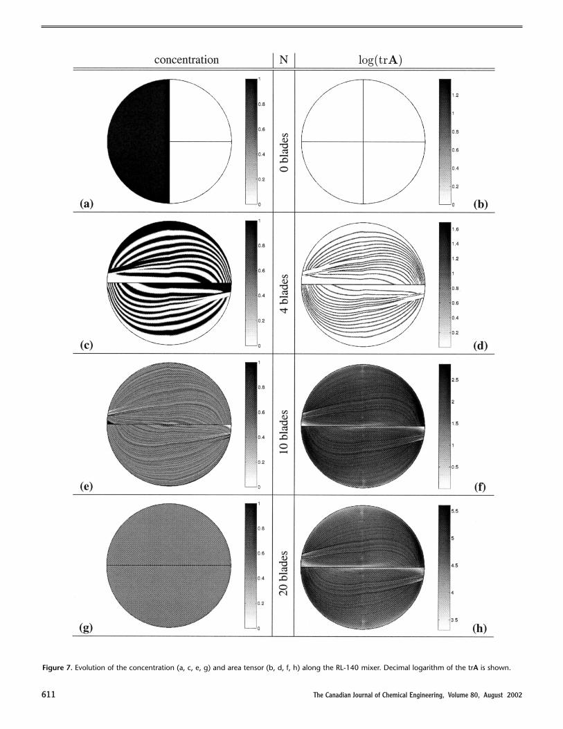
exponential growth of the interfacial area leads to the onsetof the self-similar distribution of the interfaces. It is illustrated byFigure 7, where the evolution of the concentration patterns withthe number of blades is shown for the RL-140 mixer alongsidewith the distributions of the trace of area tensor. Since the trAgrows exponentially — its logarithm is being shown — lowvalues being ignored. The self-similar distribution of interfacesis quickly established and persists after the large-scale variationsof concentration are eliminated.

It is observed that the self-similar interface distributions meanalso stable local orientation of interfaces — a phenomenon thatMuzzio et al. (1991) denoted as ‘asymptotic directionality’. InFigure 8 the striation (concentration) pattern formed after sixblades of RL-140 mixer is compared with the asymptoticorientation pattern. The latter is recovered from the area tensordistribution after 20 blades. The area tensor is averaged inrelatively big blocks (containing 2020 mapping cells) and thecorresponding eigenvalue and eigenvector problem is solved foreach average tensor. The eigenvector that corresponds to thedominant eigenvalue gives the direction of the normal tothe interface contours in the given cross-section. In Figure 8b thedashes show the actual orientation of striations (they are drawnperpendicular to the respective eigenvectors of area tensor). Itis clear that the asymptotic orientation matches the direction ofstriations formed already during initial stages of mixing.

In Figure 6 it was shown that the total interfacial area fluxgrows exponentially with the number of blades for all mixers.The values of the exponential growth rate versus pressure drop(directly linked to the number of blades for each mixer) is ofspecial interest since it characterizes the mixer efficiency in theinterface generation. Such an exponential rate of the interfacialflux generation in different RL Kenics mixers is plotted in Figure9a as a function of the blade twist angle (this exponentialgrowth rate is evaluated when the trend is firmly established —after the pressure drop, corresponding to 10 blades of RL-180mixer). The efficiency of the interface generation drops almost in

the whole investigated range of the twist angle, reaching theminimum around q = 260°. This implies that the flow withthe smallest blade twist angle q = 90° considered in this studygenerates the largest amount of interfacial area given the samepressure drop (which serves as the measure of the energyexpenses). However, for most applications not only the totalamount of inter-material interfaces is important but also theirdistribution in the bulk of the fluid. Due to the extremely widerange of the interfacial area density there is no universallyaccepted technique to evaluate the unevenness of the interfacedistribution (unlike the concentration, for which numerousstatistical measures are used). However, we try to obtain certainmeaningful characteristics of such distribution irregularity.

Computations can determine the volumetric intermaterialarea density at certain locations in the mixer cross-section as theratio between the local flux of interfacial area (see above) andthe local volumetric flux. To evaluate the irregularity of theinter-material area distribution the percentage of the fluid fluxthrough the mixer cross-section, carrying the intermaterial areadensity less than a certain threshold was estimated. The resultsare shown in Figure 9b. The relative amount of the fluid thatcrosses the cross-section of the mixer and carries less than 0.3,0.5 and 0.7 of the average interface area per unit volume isplotted. The extent of irregularity in the volumetric interfacialarea density is illustrated by Figure 10. The relative intermaterialarea density (scales with its average value) is shown respectivelyfor the RL-90 mixer that achieves highest total interfacial fluxand for RL-140 mixer that achieves the most even distribution.These results suggest that the amount of ‘bad’ flux (deprived ofinterfaces) has a clear minimum around the blade twist values140° to 150°. It means that the mixer configurations with theblades twisted 140° in alternating directions, which shows the mostefficient concentration homogenization, seems also to bethe most reasonable choice if the most even distribution of theinterfaces is sought.

Figure 6. a) The growth of the total interfacial flux with the number of blades for RL mixers with various blade twist. The marked region (contouredwith dash-dot line) is zoomed in sub-Figure (b), where additional data points, showing the interfacial area flux inside the mixing element (ratherthen at his ends), are plotted.


Figure 7. Evolution of the concentration (a, c, e, g) and area tensor (b, d, f, h) along the RL-140 mixer. Decimal logarithm of the trA is shown.


Figure 8.The asymptotic directionality in the Kenics mixer: the concentration pattern after six blades of RL-140 mixer (a) is compared with orientation,recovered using the area tensor after twenty blades (b).

Figure 9. a) The exponential rate of the interface flux growth versus the blade twist angle of RL mixer. b) The fraction of the volumetric flux of thefluid, carrying the interface density less then 0.3, 0.5 and 0.7 of the average level.

Figure 10. The relative distribution of the volumetric inter-material area density (scaled with the average value) achieved after 30 blades of RL-90mixer (a) and after 20 blades of RL- 140 mixer (a). After rather large number of blades (the total pressure drop is roughly equal for these twosituations) the self-similar distributions are already established.


Conclusions The interface generation abilities of the Kenics static mixers ofdifferent layout were studied using the extended mappingtechnique, specially adapted for these spatially periodic flows.This approach was formerly successfully used to study themicrostructure development in time-periodic, two-dimensionalprototype flows, like the lid-driven cavity and journal bearing flows.

The evolution (generation) of intermaterial interfaces wasfollowed along the mixer assuming constant-in-time feedconditions. The simulations captured the most essential features ofthe flow in static mixers, which are exponential growth of the fluxof interfacial area and its highly irregular distribution across thecross-section of the mixer. The self-similar (exponentially growing)distribution of the interfacial area density is quickly established andpersists for a long period, even after large-scale concentrationvariations are erased. The asymptotic orientation of the interfacesclosely matches the orientation of the striations visible in the initialstages of mixing.

It was found that the mixers with a small blade twist angle tendto produce a larger total amount of interfacial area at the cost of thesame pressure drop, but the produced distributions are extremelyirregular. Using the increase of interfacial area as a mixing measureto discriminate between mixers is, therefore, not very useful. It turnsout that, with the explored range of the blade twist angles, themore uniform distribution of interfaces across the mixer is achievedwhen the twist angle is close to 140° to 150°. This shows that theRL-140 mixer, which was found in our first paper (Galaktionov et al.,2002b) to achieve the most homogeneous mixture with the sameenergy input, also offer a reasonable performance in interfacial areageneration, if the most even distribution is required.

Acknowledgements The authors would like to acknowledge financial support from theDutch Polymer Institute (DPI), Project No. 161.

NomenclatureA area tensor, (m1)c relative concentration of the marked fluid–c average relative concentration of the marked fluidC vector of coarse-grain concentrationsF deformation gradient tensorF pseudo deformation gradient tensorfi volumetric flux through mapping cell number i, (m3·s–1)F total volumetric fluxI unit tensorI intensity of segregationDp pressure drop (Pa·m1)Æv local velocityWi interfacial area flux per unit area in the cell number i, (s–1)

Greek SymbolsF mapping matrixq blade twist angle

ReferencesAnderson, P.D., O.S. Galaktionov, G.W.M. Peters, F.N. Vosse and H.E.H. Meijer,

“Analysis of Mixing in Three-dimensional Time-Periodic CavityFlows”, J. Fluid Mech. 386, 149–166 (1999).

Anderson, P.D., O.S. Galaktionov, G.W.M. Peters, H.E.H. Meijer and C.L.Tucker III, “Material Stretching in Laminar Mixing Flows: ExtendedMapping Technique Applied to the Journal Bearing Flow”, Int. J.Numer. Meth. Fluids. 40(1-2), 189–196 (2002).

Aref, H., “Stirring in Chaotic Advection”, J. Fluid Mech. 143, 1–21(1984).

Ashwin, P. and G. King, “Streamline Topology in Eccentric TaylowVortex Flows. J. Fluid Mech. 285, 215–247 (1995).

Avalosse, T. and M.J. Crochet, “Finite-element Simulation of Mixing: 2.Three-dimensional Flow Through a Kenics Mixer. AIChE J. 43,588–597 (1997).

Bajer, K. and H.K. Mofatt, “On a Class of Steady Confined Stokes Flowwith Chaotic Streamlines”, J. Fluid Mech. 212, 337–363 (1990).

Danckwerts, P.V., “The Definition and Measurement of SomeCharacteristics of Mixtures”, Appl. Sci. Res. A 3, 279–296 (1953).

Feingold, M., L.P. Kadanoff and O. Piro, “Passive Scalars, 3-DimensionalVolume Preserving Maps” J. Statist. Phys. 50, 529–565 (1988).

Fountain, G.O., D.V. Khakhar, I. Mezic and J.M. Ottino, “Chaotic Mixingin a Bounded Three-dimensional Flow”, J. Fluid Mech. 417, 265–301(2000).

Galaktionov, O.S., P.D. Anderson, P.G.M. Kruijt, G.W.M. Peters andH.E.H. Meijer, “A Mapping Approach for 3D Distributive MixingAnalysis”, Comput. Fluid 30, 271–289 (2001).

Galaktionov, O.S., P.D. Anderson, G.W.M. Peters and C.L. Tucker III, “AGlobal, Multiscale Simulation of Laminar Fluid Mixing: The ExtendedMapping Method”, Int. J. Multiphase Flows 28(3), 497–523 (2002a).

Galaktionov, O.S., P.D. Anderson, G.W.M. Peters and H.E.H. Meijer,“Performance and optimization of Kenics static mixers”, Int. PolymerProcessing (Submitted) (2002b).

Hobbs, D.M. and F.J. Muzzio, “Optimization of a Static Mixer UsingDynamical System Techniques”, Chem. Engng Sci. 53(18),3199–3213 (1998).

Khakhar, D.V., J.G. Franjione and J.M. Ottino, “A Case Study of ChaoticMixing in Deterministic Flows: the Partitioned Pipe Mixer”, Chem.Engng. Sci. 42, 2909–2919 (1987).

Kruijt, P.G.M., O.S. Galaktionov, P.D. Anderson, G.W.M. Peters andH.E.H. Meijer, “Analyzing Fluid Mixing in Periodic Flows byDistribution Matrices”, AIChE J. 47, 1005–1015 (2001a).

Kruijt, P.G.M., O.S. Galaktionov, G.W.M. Peters and H.E.H. Meijer, “TheMapping Method for Mixing Optimization. part I: The MultifluxStatic Mixer”, Int. Polym. Process. XVI(2), 151–160 (2001b).

Kruijt, P.G.M., O.S. Galaktionov, G.W.M. Peters and H.E.H. Meijer, “TheMapping Method for Mixing Optimization. part II: Transport in aCorotating Twin Screw Extruder”, Int. Polym. Process. XVI(2),161–171 (2001c).

Kusch, H. and J. Ottino, “Experiments on Mixing in Continuous ChaoticFlows”, J. Fluid Mech. 236, 319–348 (1992).

Meleshko, V.V., O.S. Galaktionov, G.W.M. Peters and H.E.H. Meijer,“Three-dimensional Mixing in Stokes Flow: the Partitioned Pipe MixerProblem Revisited. Eur. J. Mech. / Part B - Fluids 18, 783–792 (1999).

Muzzio, F.J., P.D. Swanson and J.M. Ottino, “The Statistics of Stretchingand Stirring in Chaotic Flows”, Phys. Fluids A. 3, 822–834 (1991).

Ottino, J.M., “The kinematics of mixing: stretching, chaos andtransport. Cambridge texts in applied mathematics”, CambridgeUniversity Press (1989).

Peerhossaini, H., C. Castelain and Y. Leguer, “Heat-exchanger DesignBased on Chaotic Advection” Expl. Termal Fluid Sci. 7, 33–344 (1993).

Peters, G.W.M., “Tools for the Measurement of Stress and Strain Fieldsin Soft Tissue”, PhD thesis, Rijksuniversiteit Limburg te Maastricht,Maastricht, The Netherlands. (Available electronically from theMaterials Technology web-site: http://www.mate.tue.nl/ ) (1987).

Reynolds, O., “Study of Fluid Motion by Means of Coloured Bands”,.Nature 50, 161–164 (1894).

Spencer, R. and R. Wiley, “The Mixing of Very Viscous Liquids”, J. ColloidSci. 6, 133–145 (1951).

Manuscript received October 17, 2001; revised manuscript receivedMay 2, 2002; accepted for publication May 16, 2002.

morphology development in kenics static mixers

Documents

chaotic mixing

polymer mixing

effective mixing

mixing problems

cases mixing

quality of mixing

better mixing

threedimensional flows