more on dynamic programming bellman-fordfloyd-warshall wednesday, july 30 th 1

1

More on Dynamic Programming

Bellman-Ford

Floyd-Warshall

Wednesday, July 30th

2

Outline For Today

1. Bellman-Ford’s Single-Source Shortest Paths

2. Floyd-Warshall’s All-Pairs Shortest Paths

Recipe of a DP Algorithm (1)

3

1: Identify small # of subproblems

Ex 1: Find opt independent set in Gi: only n

subproblems.

Ex 2: Find optimal alignment of Xi and Yj: only mn

subproblems


4

Step 2: quickly + correctly solve “larger”

subproblems given solutions to smaller ones,

usually via a recursive formula:

Ex 1: Linear Ind. Set: A[i] = max {wi + A[i-2], A[i-

1]}

Ex 2: Alignment: A[i][j] = min

A[i-1][j-1] + αij

A[i-1][j] + δ

A[i][j-1] + δ


5

3: After solving all subproblems, can quickly

compute final solution

Ex 1: Linear Independent Set: return A[n]

Ex 2: Alignment: return A[m][n]

6

Outline For Today



7

Recap: Single-Source Shortest Paths (SSSP) Input: Directed (simple) graph G(V, E), source s, and

weights ce on edges.

Output: ∀v ∈V, shortest s v path.⤳

Dijkstra’s Algorithm: O(mlogn); only if ce ≥ 0

8

Pros/Cons of Dijkstra’s AlgorithmPros: O(mlogn) super fast & simple algorithm

Cons:1. Works only if ce ≥ 0

Sometimes need negative weights, e.g.

(finance)

2. Not very distributed/parallelizable: Looks very “serial” Need to store large parts of graph in-memory. Therefore not very scalable in very large

graphs.Bellman-Ford addresses both of these

drawbacks

(Last lecture will see parallel version of BF)

9

Preliminary: Negative Weight Cycles

Question: How to define shortest paths when

G has negative weights cycles?

s

x y

tz

4

-5

3

-6

G

10

Possible Shortest s v Path Definition 1⤳

s

x y

tz

4

-5

3

-6

G

Shortest path from s to v with cycles allowed.

Problem: Can loop forever in a negative

cycle. So there is no “shortest path”!

11

Possible Shortest s v Path Definition 2⤳

s

x y

tz

4

-5

3

-6

G

Shortest path from s to v, cycles NOT allowed.

Problem: Now well-defined. But NP-hard.

Don’t expect a “fast” algorithm solving it

exactly.

12

Solution: Assume No Negative-Weight Cycles

Q: Now, can shortest paths contain cycles?

A: No. Assume P is shortest path from s to

v, with a cycle.

P= s x⤳ x⤳ v. Then since x x is a ⤳ ⤳

cycle, and we assumed no negative weight

cycles, we could get P`= s x v, and ⤳ ⤳

get a shorter path.

13

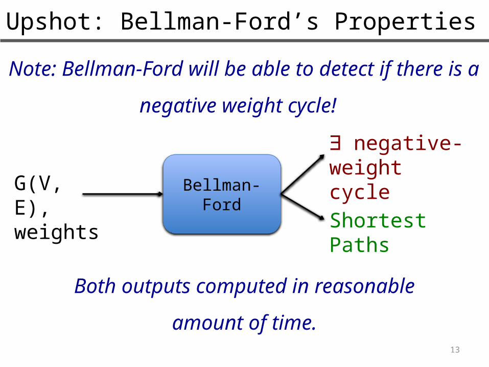
Upshot: Bellman-Ford’s Properties

Note: Bellman-Ford will be able to detect if

there is a negative weight cycle!

Bellman-Ford

G(V, E), weights

∃ negative-weight cycle

Shortest Paths

Both outputs computed in

reasonable amount of time.

14

Challenge of A DP Approach

Need to identify some sub-problems. Linear IS:

Line graph was naturally ordered from left to

right.

Subproblems could be defined as prefix graphs.

Sequence Alignment:

X, Y strands were naturally ordered strings.

Subproblems could be defined as prefix strings.

**Shortest Paths’ Input G Has No Natural

Ordering**

15

High-level Idea Of Subproblems

But the Output Is Paths & Paths Are

Sequential!

Trick: Impose an Ordering Not On G but on

Paths.

Larger Paths Will Be Derived By Appending

New Edges To The Ends Of Smaller (Shorter)

Paths.

16

Subproblems

Input: G(V, E) no negative cycles, s, ce arbitrary

weights.

Output: ∀v, global shortest paths from s to v.

Q: Max possible # hops (or # edges) on the

shortest paths?

A: n-1 (**since there are no negative

cycles**)

P(v, i) = Shortest path from s to v with

at most i edges (& no cycles).

17

Example

Let P(v, i) be the shortest s-v path with ≤ i

edges.

Q: P(t,1)?

A: Does not exist (assume such paths have ∞

weights.)

s

x

tw z

1 1

2 3 -6

a b c

-1

1 0

2

18

Example


edges.

s

x

tw z

1 1

2 3 -6

a b c

-1

1 0

2

Q: P(t,2)?

A: s->x->t with weight 2.

19

Example


edges.

s

x

tw z

1 1

2 3 -6

a b c

-1

1 0

2

Q: P(t,3)?

A: s->w->z->t with weight -1.

20

Example


edges.

s

x

tw z

1 1

2 3 -6

a b c

-1

1 0

2

Q: P(t,4)?

A: s->w->z->t with weight -1.

21

Solving P(v,i) In Terms of “Smaller” Subproblems

Let P=P(v, i) be the shortest s-v path with ≤ i edges

Note: For some v, an s-v path with ≤ i edges may

not exist. Assume v has such a path.

A Claim that does not require a

proof:

|P| ≤ i-1 OR |P| = i

22

Case 1: |P=P(v, i)| ≤ i-1

s v

Q: What can we assert about P(v, i-1)?

A: P(v, i-1) = P(v, i) (by contradiction)

(P(v, i) is also the shortest s v path with at ⤳

most i-1 edges)

23

Case 2: |P=P(v, i)| = i

Q: What can we assert about P`?

Claim: P` = P(u, i-1)

(P` is shortest s u path in with ≤ i-1 edges)⤳

s u

P`=>|s u| = i-1 ⤳

v

24

Proof that P`=P(u, i-1)

Assume ∃a better s u path Q with ≤ i-1 edges ⤳

Q had ≤ i-1 edges, then Q ∪ (u,v) has ≤ i

edges.

cost(Q) < cost(P`), cost(Q ∪ (u,v)) < cost(P).

Q.E.D

s u

Q

v

25

Summary of the 2 Cases

Case 1: |P(v, i)| ≤ i-1 => P(v, i-1) = P(v, i)

s v

Case 2: |P(v, i)| = i => P` = P(u, i-1)

s u v

P`=>|s u| = i-1 ⤳

26

Our Subproblems Agains

∀ v, and for i={1, …, n}

P(v, i): shortest s v path with ≤ i edges (or ⤳

null)

L(v, i): w(P(v, i)) (and +∞ for null paths)

L(v, i) =

min

L(v, i-1)

minu: ∃(u,v)∈E : L(u, i-1) + c(u,v)

27

Bellman-Ford Algorithm

procedure Bellman-Ford(G(V,E), weights C): Base Cases: A[0][s] =

L(v, i): w(P(v, i))

Let A be an nxn 2D array.

A[i][v] = shortest path to vertex v with ≤ i edges.

28


procedure Bellman-Ford(G(V,E), weights C): Base Cases: A[0][s] = 0 A[0][j] =

L(v, i): w(P(v, i))



29


procedure Bellman-Ford(G(V,E), weights C): Base Cases: A[0][s] = 0 A[0][j] = +∞ where j ≠ s for i = 1, …, n-1: for v ∈ V: A[i][v] = min {A[i-1][v]

min(u,v)∈E A[i-1][u]

+c(u,v)

L(v, i): w(P(v, i))



30

Correctness of BF

By induction on i and correctness of

the recurrence for L(v, i) (exercise)

31

Runtime of BF

… for i = 1, …, n-1: for v ∈ V: A[i][v] = min {A[i-1][v] min(u,v)∈E A[i-1][u]+c(u,v)

# entries in A is n2.

Q: How much time for computing each A[i][v]?

A: in-deg(v)

For each i, total work for all A[i][v] entries is:

Total Runtime: O(nm)

32

Runtime Optimization: Stopping Early

Suppose for some i ≤ n:

A[i][v] = A[i-1][v] ∀ v.

Q: What does this mean?

A: Values will not change in any later

iteration => We can stop! … for i = 1, …, n-1: for v ∈ V: A[i][v] = min {A[i-1][v] min(u,v)∈E A[i-1][u]+c(u,v)

Values only depend on the previous iteration!

33

Negative Cycle Checking

Consider any graph G(V, E) with arbitrary edge

weights.

=>There may be negative cycles.

Claim: If BF stabilizes at some iteration i > 0,

then G has no negative cycles.

(i.e., negative cycles implies BF never

stabilizes!)

34

How To Check For Cycles If Claim is True

Run BF just one extra iteration!

Check if A[n][v] = A[n-1][v] for all v.

If so, no negative cycles, o.w. there is a

negative cycle.

Running n iterations is the general form of BF:

Bellman-Ford

G(V, E), weights

∃ negative-weight cycle

Shortest Paths

35

Proof of Claim: BF Stabilizes => G has no negative

cyclesAssume BF has stabilized in iteration i.

Notation: d(v) = A[i][v] = A[i-1][v] (by above

assumption)A[i][v] = min {A[i-1][v] min(u,v)∈E A[i-1][u] + c(u,v)

d(v) = min {d(v) min(u,v)∈E d(u) + c(u,v)

d(v) ≤ d(u) + c(u,v)

Let’s argue that every cycle C has non-negative weight...

36

Proof of Claim (continued)

d(v) ≤ d(u) + c(u,v)

Fix a cycle C:y

x

z

t

37


d(v) ≤ d(u) + c(u,v) => d(v) – d(u) ≤ c(u,v)

Fix a cycle C:y

x

z

t

38


d(v) ≤ d(u) + c(u,v) => d(v) – d(u) ≤ c(u,v)

Fix a cycle C:y

x

z

t

d(x) – d(t) ≤ c(t,x)

39


d(v) ≤ d(u) + c(u,v) => d(v) – d(u) ≤ c(u,v)

Fix a cycle C:y

x

z

t

d(x) – d(t) ≤ c(t,x)

d(y) – d(x) ≤ c(x,y)

40


d(v) ≤ d(u) + c(u,v) => d(v) – d(u) ≤ c(u,v)

Fix a cycle C:y

x

z

t

d(x) – d(t) ≤ c(t,x)

d(y) – d(x) ≤ c(x,y)

d(z) – d(y) ≤ c(y,z)

41


d(v) ≤ d(u) + c(u,v) => d(v) – d(u) ≤ c(u,v)

Fix a cycle C:y

x

z

t

d(x) – d(t) ≤ c(t,x)

d(y) – d(x) ≤ c(x,y)

d(z) – d(y) ≤ c(y,z)

d(t) – d(z) ≤ c(z,t)

0 ≤ w(C) Q.E.D.

Same algebra and result for any cycle

(exercise).

42

Space Optimization (1)


Only need A[i-1][v]’s to compute A[i][v]s.

Only need O(n) space; i.e., O(1) per vertex.

Q: By throwing things out, what do we lose in

general?

A: Reconstruction of the actual paths.

But with only O(n) more space, we can actually

reconstruct the paths!

43

Space Optimization (1)


Fix: Each v stores a predecessor pointer (initially

null)

Whenever A[i][v] is updated to A[i-1][u]+c(u,v), we

set the Pred[v] to u.

Claim: At termination, tracing pointers back from

v yields the shortest s-v path.

(Details in the book, by induction on i)

44

Summary of BF

Runtime: O(nm), not as fast as Dijkstra’s

O(mlogn).

But works with negative weight edges.

And is distributable/parallelizable.

Will see its distributed version last lecture of

class.

45

Outline For Today



46

All-Pairs Shortest Paths (APSP)

Input: Directed G(V, E), arbitrary edge weights, no neg.

cycles.

Output: ∀ u, v, d(u, v): shortest (u, v) path in G.

(no fixed source s)

Q: What’s a poly-time algorithm to solve

APSP?

A: for each s, run BF from s => O(n2m)

Better Algorithm: Floyd-Warshall

47

Floyd-Warshall Idea

Linear IS: input graph naturally ordered

sequentially

Seq. Alignment: strings naturally ordered

sequentially

Bellman-Ford: output paths naturally ordered

sequentially

FW imposes sequentiality on the vertices

order vertices from 1 to n

only use the first i vertices in each subproblem

(Same idea works for SSSP, but less efficient than

BF.)

48

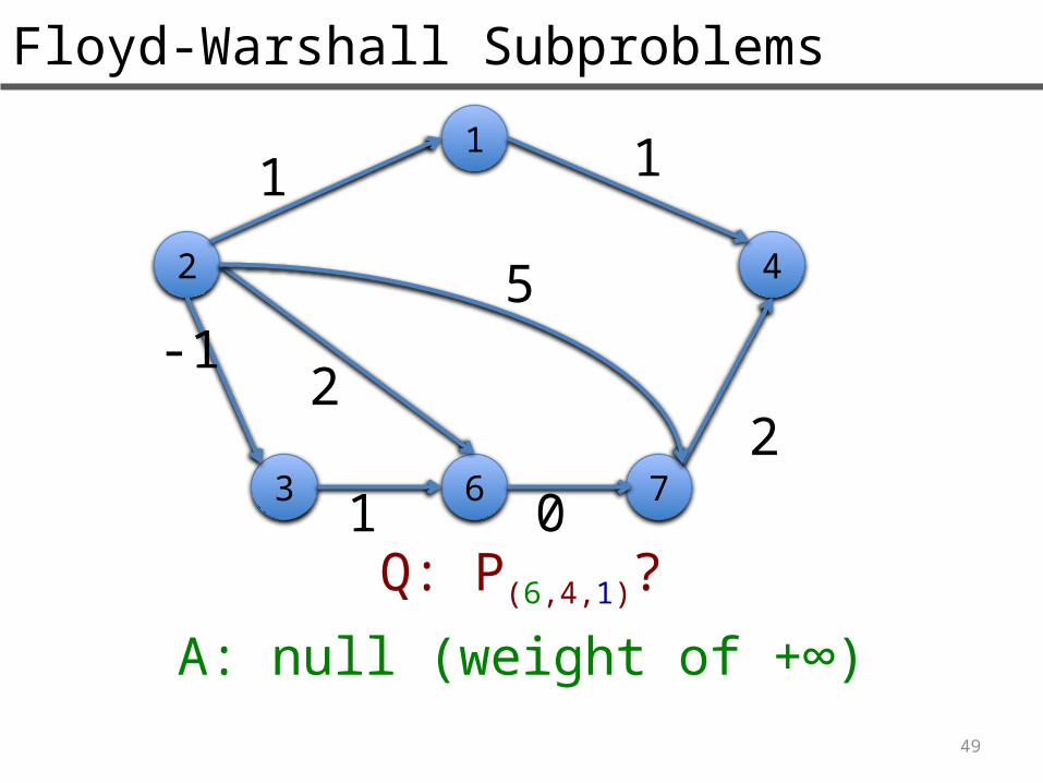
Floyd-Warshall Subproblems

V= {1, …, n}, ordered completely arbitrarily

Vk = {1, …, k}

Original Problem: ∀(u, v) shortest u, v path.

We need to define the subproblems.

Subproblem P(i, j, k) = shortest i, j path that uses

only Vk as intermediate nodes (excluding i and

j).

49


2

1

4

1 1

2

3 6 7

-1

1 0

2

5

Q: P(6,4,1)?

A: null (weight of +∞)

50


2

1

4

1 1

2

3 6 7

-1

1 0

2

Q: P(2,4,1)?

A: 2->1->4 (weight of 2)

5

51


2

1

4

1 1

2

3 6 7

-1

1 0

2

Q: P(2,6,0)?

A: 2-6 (weight of 2)(no intermediate nodes needed)

5

52


2

1

4

1 1

2

3 6 7

-1

1 0

2

Q: P(2,6,1)?

A: 2-6 (still weight of 2)(without intermediate nodes)

5

53


2

1

4

1 1

2

3 6 7

-1

1 0

2

Q: P(2,6,2)?

A: 2-6 (still weight of 2)(without intermediate nodes)

5

54


2

1

4

1 1

2

3 6 7

-1

1 0

2

Q: P(2,6,3)?

A: 2->3->6 (weight of 0)(now with intermediate node 3)

5

55


2

1

4

1 1

2

3 6 7

-1

1 0

2

Final shortest i⤳j path is P(i, j, n)

when we’re allowed to use any vertices as intermediate nodes.

5

56

Claim That Doesn’t Require A Proof

Fix source i, and destination j

k ∉ P(i, j, k) OR k∈P(i, j, k)

i j

(either one of the intermediate vertices is k or it’s

not)

57

Case 1: k ∉ P(i, j, k)

Then all internal nodes are from 1,

…,k-1.

Q: What can we assert about P(i, j, k)? i j

all intermediate vertices are from Vk-1

A: P(i, j, k) = P(i, j, k-1)

(proof by contradiction)

58

Case 2: k ∈ P(i, j, k)

Q: What can we assert about P1 and

P2? i jk

one (and only one) of the int. nodes is k. (why only

one?)A1: P1 & P2 only contain int. nodes 1,

…,k-1

A2: P1 = P(i,k,k-1) & P2 = P(k,j,k-1)

(proof by contradiction)

P1

P2

59

Summary of the 2 Cases

Case 1: k ∉ P(i, j, k) => P(i, j, k) = P(i, j, k-1)

Case 2: k ∈ P(i, j, k) => P1 = P(i,k,k-1) & P2 =

P(k,j,k-1)

i j

i jk

P1

P2

60

Recurrence for Larger Subproblems

∀ i, j, k and where i,j,k={1, …, n}

P(i, j, k): shortest i j path with all ⤳

intermediate nodes from Vk={1,…,k} (or

null)

L(i, j, k): w(P(i, j, k)) (and +∞ for null paths)

L(i, j, k) =

min

L(i, j, k-1)

L(i, k, k-1) + L(k, j, k-1)

With appropriate

base cases.

61

Floyd-Warshall Algorithm

procedure Floyd-Warshall(G(V,E), weights C): Base Cases: A[i][i][0]

Let A be an nxnxn 3D array.

A[i][j][k] = shortest i j path with V⤳ k as intermediate

nodes

62


procedure Floyd-Warshall(G(V,E), weights C): Base Cases: A[i][i][0] = 0 A[i][j][0] =



nodes

63


procedure Floyd-Warshall(G(V,E), weights C): Base Cases: A[i][i][0] = 0 A[i][j][0] = Ci,j if (i,j) ∈ E

+∞ if (i,j) ∉ E for k = 1, …, n: for i = 1, …, n: for j = 1, …, n:

A[i][j][k] = min {A[i][j][k-1], A[i][k][k-1] + A[k][j][k-1]}



nodes

64

Correctness & Runtime

procedure Floyd-Warshall(G(V,E), weights C): Base Cases: A[i][i][0] = 0 A[i][j][0] = Ci,j if (i,j) ∈ E

+∞ if (i,j) ∉ E for k = 1, …, n: for i = 1, …, n: for j = 1, …, n:

A[i][j][k] = min {A[i][j][k-1], A[i][k][k-1] + A[k][j][k-1]}

Correctness: induction on i,j,k & correctness of

recurrence

Runtime: O(n3) (b/c n3 subproblems, O(1) for each

one)

65

Detecting Negative Cycles

Just check the A[i][i][n] for each i!

Let C be a negative cycle with |C| = l

=>for any vertex j on C, A[j][j][l] ≤ 0

=> therefore A[j][j][n] will be negative

66

Path Reconstruction

Similar to BF but keep successors

instead of predecessors.

(exercise)

67

Dijkstra, BF, FW

Dijkstra BF FW

Single-Source /All Pairs

Single-Source

Single-Source

All Pairs

Run-time O(mlog(n))

O(mn) O(n3)

Negative Edges

No Yes Yes

Negative Cycles

No No, but can detect

No, but can detect

68

Will see a parallel version of BF in last

lecture.

Next Week: Intractability, P vs NP &

What to Do for NP-hard Problems?

more on dynamic programming bellman-fordfloyd-warshall wednesday, july 30 th 1

Documents

paths paths

g slide

g shortest path

shortest s v path

shortest paths input

amn slide

mn subproblems slide

larger paths