Moral Hazard and International CrisisLending: A Test∗

(preliminary and incomplete, do not quote without permission)

Giovanni Dell�AricciaInternational Monetary Fund

Isabel GoddeUniversity of Mannheim

Jeromin ZettelmeyerInternational Monetary Fund

November 7, 2000

Abstract

This paper examines how events that change expectations aboutfuture international crisis lending modify the relationship betweencountry spreads and fundamentals. If moral hazard is present, suchevents should affect the level of spreads, the sensitivity with whichspreads reßect fundamentals, and their cross-country dispersion. Whenapplied to the Russian crisis of 1998, these tests Þnd strong evidenceconsistent with the existence of moral hazard. However, this evidenceis subject to a fundamental interpretational caveat: the same Þndingscould also be attributed to the perception that international crisislending reduces the true risk of Þnancial crises in emerging markets.

∗We would like to thank Eduardo Borensztein and Olivier Jeanne for useful discussionsand suggestions, and Manzoor Gill for help in compiling the data set. All the errors areours. The views expressed in this paper are those of the authors and do not necessarilyreßect those of the IMF.

1

1 Introduction

The role of international Þnancial rescue operations in causing �moral hazard��resulting in overinvestment or insufficient monitoring by investors, bad poli-cies on the side of governments, or both�has been at the center of debateever since the 1995 Mexican bail-out.1 Participants in this debate disagreeabout the extent to which this type of moral hazard has caused problemsin the past, with views ranging from the belief that the Mexican rescue�caused� the Asian crisis to the idea that moral hazard due to the expecta-tion of international crisis lending is an isolated phenomenon associated withparticular large borrowers. However, concern about its potential impact isshared almost universally, even by those who would defend the large bail-outsof the 1990s. Indeed,�limiting moral hazard to the extent possible� appearsto have become an explicit policy objective of the International MonetaryFund. One reßection of this objective is a consensus among official creditorsto enforce greater private sector �burden-sharing� as a complement to officialassistance.2

Given this near-universal concern, it comes as something of a surprise thatthere exists little empirical work on the subject, and that the few studies thathave systematically tested for moral hazard have found either no or highlyambivalent evidence for its existence.3 As we will argue in this study, someof this ambivalence is intrinsic to the subject and unavoidable, but a goodportion of it is not. The objective of this paper is to take a fresh look atthe evidence in ways that go beyond the existing literature in three respects:Þrst, by exploiting a wider range of testable implications of moral hazard,second, by making an attempt to disentangle moral hazard from alternativeexplanations of the phenomena that might be viewed as reßecting moralhazard, and�last not least�by using a broader range of data. Like the

1See, for example, Calomiris (1998), Meltzer (1998), and Willett (1999).2See �Report of the Managing Director to the International Monetary and Financial

Committee on Progress in Strenghtening the Architecture of the International FinancialSystem and Reform of the IMF�, September 19, 2000, �IMF Executive Board DiscussesInvolving the Private Sector in the Resolution of Financial Crises�, Public Information No-tice (PIN) No. 00/80, International Monetary Fund, September 19, 2000 (both documentsavailable on the IMF�s Website, www.imf.org) .

3See Zhang (1999), Nunnenkamp (1999), Willett (1999), Lane and Phillips (2000), anda related paper by Jeanne and Zettelmeyer (2000), who do not take a position on the overallempirical signiÞcance of moral hazard, but argue that the subsidy element associated withinternational bail-outs is small.

2

previous literature, we exploit the idea that a change in moral hazard shouldtranslate into a change in emerging market bond spreads if moral hazard wasin fact present. Our main methodological innovation is that we do not onlyexamine how this affects the level of spreads, but also their cross-countrydispersion, and the sensitivity with which they reßect fundamentals.Unlike the earlier literature, our tests do Þnd strong evidence consis-

tent with the existence of moral hazard. However, this evidence is subjectto a fundamental interpretational caveat which we share with the previousliterature. In principle, our Þndings could be attributed both to the percep-tion that international crisis lending reduces the probability that investorswill suffer losses, conditioning on a Þnancial crisis in emerging markets, andto the perception that international crisis lending reduces the true risk ofemerging market crises.4

To our knowledge, there are only two earlier studies that attempt a sys-tematic empirical test of moral hazard: Zhang (1999) and Lane and Phillips(2000).5 Lane and Phillips (2000) examine the reactions of a daily emergingmarket bond index to a large number of events that might have changedexpectations of future international crisis lending. In most instances, theydo not Þnd evidence consistent with the presence of moral hazard, in thesense that spreads do not seem to react to the events in question. In somecases�in particular, the Russian default in August 1998, which was notablefor the absence of an international rescue when it was expected�they do.The problem is that these Þndings have ambivalent interpretations, as Laneand Phillips themselves point out. Failure to detect a signiÞcant reaction ofspreads could always be due to the fact that the event was already antic-ipated. As to the large reaction to the Russian default, this could reßectinvestor panic, contagion, and liquidity changes, making it impossible to at-tribute investors� reactions to changes in the perceived probability of futurecrisis lending, as opposed to momentary Þnancial market turbulence.In principle, this problem can be tackled through the methodology used

by Zhang (1999), who analyzes the longer-term impact of an event that hasbeen often associated with an increase in moral hazard�the 1995 Mexicanbail-out�while controlling for changes in some macroeconomic fundamentalsand a measure of international liquidity (namely, the spread on high-yield US

4This point is made extensively by Lane and Phillips (2000).5Demirguc-Kunt and Huizinga (2000) test for moral hazard in the bank deposit market

induced by deposit insurance schemes. Their methodology is analogous to that in Zhang(1999) described below.

3

corporate bonds). His main result is that a post-Mexico dummy is insignif-icant and has the wrong sign (positive, rather than negative as one wouldexpect if moral hazard had depressed spreads). However, this result is basedon one single event, which arguably is not very well suited to a test of moralhazard. If the Mexican crisis led to a general reassessment of risks relatedto emerging market lending�as investors learned that even a country witha recent track record of reform and relatively sound fundamentals could ex-perience a disastrous Þnancial crisis�any reduction in spreads due to moralhazard may have been offset by a general increase in the perceived riskinessof sovereign debt. Moreover, Zhang�s test fails to exploit testable implica-tions that moral hazard has for the slope coefficients, rather than just theintercept, of his regression equation (see next section).Our study shares Zhang�s basic approach in the sense of testing for moral

hazard in the context of a regression model of spread determination. How-ever, we differ along two dimensions, which turn out to (jointly) make adifference to the results.First, rather than just looking at the impact on the average level of

spreads, which is the focus of the previous literature, we test whether theRussian crisis led to (1) changes in the level of spreads in a wide range ofindividual countries; (2) changes in the sensitivity with which spreads reactto fundamentals,6 and Þnally, (3) changes in the cross-country variance ofspreads (always controlling for fundamentals). In the context of a simplemodel of international lending (section 2.2 of this paper), these are shownto be testable implications of the presence of moral hazard (subject to thebasic interpretational caveat referred to earlier).Second, while we also apply our test to the Mexican bail-out to compare

our results to the earlier literature, the main focus is on the Russian crisis,which we argue constitutes a better experiment for the purpose of testing formoral hazard. To ensure that our results are not driven by contagion or liq-uidity effects, we disregard the immediate reaction of spreads to the Russiandefault, and instead compare monthly or quarterly spreads before and wellafter the crisis (namely, after emerging market turbulence had subsided in theÞrst quarter of 1999). This requires carefully controlling for �fundamentals�that may affect spreads, and that may have changed in the meantime. We dothis using a model of spread determination encompassing most fundamentals

6Kamin and Kleist (1999) carry out a similar test in a regression with only one riskfactor (credit ratings) without interpreting their procedure as a test for moral hazard.

4

that have been suggested in the literature on bond pricing.7

There are two main Þndings. First, the Russian crisis led to a signiÞ-cant and sustained increase in spreads in many, but not all, emerging marketcountries studied, in particular in countries with relatively weak fundamen-tals. Second, the crisis led to large increase in the cross-sectional dispersionof spreads, controlling for fundamentals. In other words, investors seem tohave paid much more attention to differences in individual country charac-teristics after the crisis than they had done before.The remainder of the paper is organized as follows. Section 2 derives

several alternative testable implications of the presence of moral hazard inthe context of a simple model of international lending. Section 3 discusses theimplementation of these tests in the context of an empirical model of spreaddetermination, as well as the validity of the Russian crisis as an �experiment�for our purposes. Section 4 presents our results, which are based on twodistinct datasets: J.P. Morgan�s dataset of secondary market bond spreadscontained in the �EMBI Global� Bond Index, and an exhaustive datasetof launch bond spreads based on Capital Data�s �Bondware�. Section 5interprets the results, and concludes.

2 A Simple Model

Suppose one had a clear-cut event affecting the perceived likelihood of fu-ture official crisis lending to emerging market economies. Then, it should bepossible to use Þnancial market reactions to such an event�in particular,changes in emerging market bond spreads�to test for the presence of moralhazard attributable to international Þnancial rescues. This section presentsa simple model of a competitive credit market facing heterogenous borrowercountries and derives several testable implications of moral hazard. Method-ological issues related to the implementation of these tests�in particular,what events, if any, could be used as a natural experiment for our purposes,as well as issues related to econometric modeling�are left to the next section.

2.1 Set-Up

Consider a world where multiple, risk-neutral lenders (investors) competefor loans in hard currency (say US$) to borrower countries. Countries are

7See, in particular, Cline and Barnes (1997) and Eichengreen and Mody (1998).

5

heterogeneous in terms of observable country-speciÞc fundamentals, xi (acountry-speciÞc vector), which in turn affect their perceived probability ofdefault. The latter can be decomposed into the probability of incurring aÞnancial crisis, θ, and investors� perceived probability of being repaid, λ, i.e.avoidance of default, conditional on a crisis. This enables us to write the riskfrom the perspective of the individual investor as (1−λ)θ. Denoting the riskfree rate as R∗ (assumed constant), the equilibrium interest rate then followsfrom the no-arbitrage condition and can be written as:8

Ri =R∗

1− (1− λ (xi))θ(xi)Now introduce the possibility of international crisis lending a la Mexico(1995) or Korea (1997). Let b denote the perceived probability that a coun-try will receive an international rescue package in the event of a crisis. Ingeneral, this may affect emerging market yields through three channels:

� it might affect observable fundamentals, in particular through govern-ment policies: xi = xi(b);

� it might affect the conditional repayment probability: λ = λ (xi, b) ;� Þnally, it might affect the probability of a Þnancial crisis, conditioningon fundamentals: θ = θ(xi, b). For example, the presence of an inter-national Þnancial �safety net� might reduce the probability of liquiditycrises.

�Country moral hazard� usually refers to the Þrst of these effects, i.e.the deterioration of the borrower country policies in the face of a Þnancialsafety net. �Investor moral hazard� is typically identiÞed with the secondeffect�an increase in the probability that investors will go scot-free in theevent of a crisis�and this is the sense in which the term will be used in thediscussion that follows.9 More formally, we speak of �investor moral hazard�

8Throughout the paper R indicates gross interest rates; in other words, R = 1 + r,where r is the net interest rate.

9Strictly speaking, this is loose language, since �investor moral hazard��in analogy tothe deÞnition of �country moral hazard� just suggested�should refer to socially inefficientinvestor actions (for example, excess lending, or insufficient monitoring) rather than anincrease in the conditional repayment probability per se. However, it is clear that in astandard set-up that explicitly model these actions, an increase in the conditional repay-ment probability would have precisely this effect, since it would insulate investors fromthe risk of a Þnancial crisis, θ.

6

if the following property holds:

∂λ (xi, b)

∂b> 0 (1)

At Þrst sight, this condition might appear to be inevitably satisÞed. How-ever, international rescue packages do not necessarily involve the bail-out ofprivate international investors. On the contrary, on a number of occasionsprivate creditors suffered substantial �haircuts�. Still, a higher probabilityof international Þnancial rescues may be perceived as increasing the proba-bility of international bail-outs, and it is through that perception that rescuepackages may cause moral hazard. Thus, we speak of investor moral hazardif an increase in the probability of an international rescue increases investors�expectations of being bailed-out in case of a Þnancial crisis.In the remainder of the paper, we focus on �investor moral hazard� while

abstracting from �country moral hazard�, i.e. taking xi as given (in our em-pirical work, this means controlling for changes in xi). The central questionis how to test for investor moral hazard when λ is not directly observable.Below, we present a restricted model from which three testable implicationsof investor moral hazard are derived. In the Appendix, we discuss how theproperties of those tests are affected when the restricting assumptions arerelaxed.

2.2 Testable Implications of �Investor Moral Hazard�

Consider the following specialization of the model sketched above, which forconvenience has been rewritten in terms of emerging market spreads si ≡Ri −R∗, rather than yields.First, assume that the probability of a Þnancial crisis, θ, is not directly

affected by changes in b, i.e.:

∂θ(xi, b)

∂b= 0 , (2)

so that we can write

si = R∗ (1− λ (xi, b))θ(xi)1− (1− λ (xi, b))θ(xi) . (3)

7

Second, assume that to the extent that an increase in b affects the ex-pected conditional repayment probability�i.e. generates investor moral hazard�it does so uniformly across countries:

∂2λ

∂xi∂b= 0 . (4)

In this restricted set-up, we can state three equivalent testable impli-cations of investor moral hazard. For a given set of fundamentals, an in-crease (decrease) in the perceived likelihood of an international rescue i)reduces (increases) the level of spreads; ii) reduces (increases) the sensitivityof spreads to changes in fundamentals; iii) reduces (increases) the differ-ence in the spreads between any pair of countries (with initial spreads �closeenough�).More formally, the Þrst result can be written as (omitting the country

subscripts)

Proposition 1 Holding constant the set of fundamentals X = (x1,x2, ...xn),conditions (2) and (4) imply that dλ

db> 0 if and only if ds

db< 0.

Proof: see Appendix. ¥

An increase in the probability of rescues results in a lower perceived riskassociated with international lending, reducing country spreads across theboard. Under the stated conditions, this directly provides a test for moralhazard. Innovations that increase investor moral hazard (like large IMFbail-outs) should result into lower spreads, after controlling for the effect ofchanges in the fundamentals. We will refer to the test based on proposition1 as the �level test�.Assuming that fundamentals are deÞned such that θ is increasing in all

the components of xi (in other words, all fundamentals are expressed as �riskfactors�) we can state our second result as follows:

Proposition 2 Conditions (2) and (4) imply that dλdb> 0 if and only if

d2sidxijdb

< 0 for every j.

Proof: see Appendix. ¥

From an investor�s standpoint, a higher probability of getting off �scot-free� makes the idiosyncratic characteristics of each country less important,

8

weakening the link between fundamentals and interest rate spreads (in theextreme, with λ = 1, all countries would pay the same risk-free interest rateregardless of their fundamentals). This proposition provides a second testfor investor moral hazard. Events that increase moral hazard should reducethe size of the slope coefficients linking country spreads and fundamentals.We will refer to this test as the �slope test�.Finally, deÞne ∆s = s1− s2, where s1 and s2 are the interest rate spreads

of any two countries. If s1 and s2 are �close enough� in the sense that ∆scan be approximated by a Taylor expansion, then we can prove the followingproposition:

Proposition 3 Holding constant the set of fundamentals (x1,x2, ...xn), con-ditions (2) and (4) imply that dλ

db> 0 if and only if d∆s

db< 0 for any s1, s2.

Proof: see Appendix. ¥

This proposition shows that, for any given set of fundamentals, the dis-persion of the interest rate spreads decreases when investor moral hazardincreases. Intuitively, since moral hazard implies that investors pay less at-tention to differences in fundamentals across countries, the differences be-tween country spreads should also narrow.This result implies that an increase in investor moral hazard reduces the

cross-sectional variance of the spreads. In the empirical part of this paperwe exploit this property in constructing our �variance test�.Under assumptions (2) and (4), the propositions in this section show three

necessary and sufficient conditions for investor moral hazard, providing threealternative and equivalent testable implications. However, when the assump-tions are relaxed, the three conditions cease to be sufficient and remain onlynecessary. At the same time, the equivalence among the three tests ceasesto exist.A particularly interesting case is one where instead of assuming that the

probability of a Þnancial crisis, θ, does not depend on the rescue probabil-ity b, one allows for an ex-ante beneÞcial role of international crisis lending.For example, crisis lending may help coordinate investors and prevent pan-ics, reducing the probability of liquidity crises.10 In the Appendix, we showthat in this case, the �level� test will never be able to distinguish the ef-fects of investor moral hazard from those of true risk reduction and that the

10In that case, we would have ∂θ(xi,b)∂b < 0.

9

�slope� and �variance� tests can make this distinction only under conditionsthat are not necessarily satisÞed in practice. Thus, the inability to unam-biguously distinguish moral hazard from true risk reduction attributable tointernational crisis lending is a fundamental identiÞcation problem which isnot easily resolved, and must be kept in mind when interpreting the results.

3 Empirical Methodology

3.1 Regression-based tests for moral hazard

We start from a standard model of the determination of bond spreads

sijt = Xβ + uijt

= β0 +Xijtβ1 +Xitβ2 +Xiβ3 +Xtβ4 + uijt, (5)

where sijt denotes the spread of bond j of country i in time t, and X denotesthe matrix of fundamentals that determine the spreads of sovereign bonds.These fundamentals might be bond-, country-, and/or time-speciÞc. Theterm u represents a random error. This equation will be the basis of all ourregressions.Consider now an event that reduces the perceived probability of future

bail-outs.11 The general estimation procedure will be to estimate a pooledmodel over the whole period, i.e. before and after the event, without restrict-ing the coefficients of the model to be the same before and after the event.Thus, bond spreads before the event can be described by the model

s = Xβ + u, (6)

while the model changes to

s∗ = X∗β∗ + u∗ (7)

after the event due to a potential structural break. Denoting H0 the nullhypothesis that moral hazard is not present, and H1 the presence of moral

11Since we are looking at the unexpected absence of a further international rescue pack-age for Russia in August of 1998, this is the relevant case for our empirical analysis.

10

hazard, the three tests derived in our theoretical framework can be restatedas follows in the context of the empirical model:12

1. Under H0, the slopes of the regression equation should be unaffected byan event that reduces expected international crisis lending. Under H1,however, we would expect all slopes to increase (in absolute value) afterthe event because investors bear a larger part of the repayment risk andwill price risk factors more than before. This is the test referred to asthe slope test in section 2. It can be carried out as a simple t test onthe signiÞcance of the change of each individual slope.13 In the caseof an event that decreases moral hazard, the test can be formulated asfollows:

H0 : |β∗k − βk| = 0, k = 1, ...K

H1 : |β∗k − βk| > 0, k = 1, ...K

Note that this test refers only to the slopes of the regression and notto the intercept.14

2. Under H0 (i.e. no moral hazard), the level of spreads should not beaffected by an event that reduces expected international crisis lending.Under H1 (i.e. moral hazard), however, the level of spreads shouldincrease for every country, holding fundamentals constant. More for-mally, the change in the level of spreads can be decomposed into threecomponents:

s∗ − s= X∗(β∗ − β) + (X∗ −X)β + (u∗ − u) (8)

= X(β∗ − β) + (X∗ −X)β∗ + (u∗ − u)12As has been outlined above, we have to assume that the expectation of reduced future

crisis lending has no direct risk-increasing effect. If this assumption is not made, all testshave to be reinterpreted as tests of the joint hypothesis that either moral hazard or a truerisk-increasing effect is present, or both.13A similar test can be found in the paper by Kamin and Kleist (1999).14Our model predicts that the �theoretical intercept�, i.e. the spread at θ = 0 is equal

to zero irrespective of the occurrence of international bail-outs. The intercept of our re-gression, however, is not identical to this theoretical intercept. Therefore, the implicationsfor the �empirical intercept� are not obvious.

11

The Þrst term is the change in the level of spreads induced by thechange in β, the second term the change in the level of spreads causedby the change in the fundamentals, and the third term reßects theimpact of a change in the error term.15 Here, we are only interested inthe Þrst term, which captures the effect of a change in the pricing ofrisks on the level of spreads. Thus, in the case where the event entailsa potential decrease in moral hazard, the level test takes the followingform:

H0 : eX(β∗ − β) = 0H1 : eX(β∗ − β) > 0

The test can be carried out as a linear Wald test in which we comparethe Þtted spreads that result from the models estimated before and afterthe event.16 Note that the above decomposition and thus the choice ofeX are not unique: when controlling for fundamentals, one can eitheruse the fundamentals before or after the event. In fact, this choice canaffect the results of the test. Therefore, we present the results for bothchoices.

3. Under H0, the cross-sectional variance of the spreads should remainunchanged after the event. UnderH1, however, the difference in spreadsbetween each pair of countries should increase, which, in turn, impliesan increase in the cross-sectional variance of spreads (controlling forchanges in fundamentals).We refer to this test as the variance test.More formally, we can write the variance before the event as

V ar(s) = β 0V ar(X)β + σ2 (9)

and the variance after the event as

V ar(s∗) = β∗0V ar(X∗)β∗ + σ∗2, (10)

15This is the well-known Oaxaca decomposition that has also been used by Eichengreenand Mody (1998).16This test is very different from the one employed by Zhang (1999) who allows only

the intercept to change after the event. Thus, Zhang assumes that the coefficients onfundamentals are unchanged before and after the event, which would not be true if moralhazard were in fact present (see Section 2).

12

where σ2 and σ∗2 are the variances of the error terms. The change inthe variance of spreads can be decomposed into three components:

V ar(s∗)− V ar(s)= [β∗0V ar(X∗)β∗ − β0V ar(X∗)β] +

[β 0V ar(X∗)β − β 0V ar(X)β] + £σ∗2 − σ2¤ (11)

= [β∗0V ar(X)β∗ − β 0V ar(X)β] +[β∗0V ar(X∗)β∗ − β∗0V ar(X)β∗] + £σ∗2 − σ2¤

The Þrst term is the change in the variance induced by the change inβ, the second term the change in the variance caused by the change inthe fundamentals, and the third term reßects the impact of a changein the variance of the error term.17 Again, we are mainly interested inthe Þrst term, which captures the effect of a change in the pricing ofrisks on the variance of spreads. Thus, if the event entails a potentialdecrease in moral hazard, the variance test takes the following form:

H0 : β∗0V ar( eX)β∗ = β 0V ar( eX)βH1 : β∗0V ar( eX)β∗ > β 0V ar( eX)β

The variance test will be carried out as a nonlinear Wald test (see Ap-pendix for statistical details). Note that the above decomposition is again

not unique: the choice of eX can affect the results of the test, and we showresults for both alternatives.It is important to clarify the relations between our three tests. If all slopes

increase in absolute value, the variance is also going to increase and so is thelevel (unless there is a decrease in the intercept strong enough to reversethe effect of the slopes). Thus, there is no point in doing all three tests inthis situation. The interesting case is one in which some, but not all slopesshow signiÞcant increases, while some may even show decreases. In the slopetest, this would imply a rejection of H0, which predicted no change in slopes.However, this rejection would not be very convincing if the increase in someslopes were accompanied by decreases in others. Indeed, H1 predicts thatall slopes should increase. The question is whether the slope coefficientsshowing signiÞcant increases �outweigh� those showing decreases, so that

17This type of decomposition is well-known in the labor literature on the evolution ofthe distribution of incomes over time.

13

we can accept the presence of moral hazard with some conÞdence insteadof concluding, for example, that the regression model is misspeciÞed or theexperimental event is ambiguous, so that no lessons can be drawn.How should one decide whether the positive slope movements outweigh

the negative ones? One natural way of weighing the slopes is to look at theimpact of the change of the slopes on Þtted spreads, controlling for funda-mentals. This is the logic behind the level test. Unfortunately, the resultsfrom this test also are very unlikely to be unambiguous. First, the resultsfrom this test may differ across countries and second, the choice of eX mayaffect the test results. Therefore, we also employ the variance test, which al-lows us to summarize the overall effect of the changing slopes on all countriesin a way suggested by our model.Some caveats remain with respect to the interpretation of the variance

test. First, there continues to be an ambiguity with respect to the choice of eX.Second, it is important to note that a rejection of the null hypothesis in thevariance test does not require all Þtted spreads to go up. For the variance test,the direction of the change in Þtted spread is irrelevant as long as the spreadsmove farther apart from each other. Third, our theoretical model predictsthat the increase in the variance is driven by an increase in the distance ofneighboring spreads, with the �order� of countries being unchanged. Yet,the order of countries does not enter the variance test. Therefore, the resultsfrom the variance test can only be interpreted in combination with the resultsfrom the level test. Indeed, while the increase of the cross-sectional varianceis a necessary condition of moral hazard, it is not a sufficient one.

3.2 The Russian crisis as a valid experiment

A critical element of our testing strategy for moral hazard is the choice of anevent that constitutes a valid experiment for the purpose of the test. Suchan event has to satisfy three conditions:

1. It has to change the public perception of the extent and/or the char-acter of future international crisis lending.

2. It has to be unexpected.

3. It must not lead to a reassessment of risks other than through theexpectations of future international rescues.

14

We believe that the events following the Russian default in August 1998satisfy all three conditions reasonably well. The Russian crisis unfolded whenthe Russian authorities announced a de facto devaluation of the ruble, a uni-lateral restructuring of ruble-denominated public debt, and a moratorium onforeign debt repayments on August 17, 1998. Clearly, this did not constitutenews about the poor state of the Russian economy; in fact, Russia had beendowngraded by all three major rating agencies in the Þrst half of 1998, whichsuggests that investors were well aware of the increasing economic risks.The real surprise was that the international community did not prevent

the default of a country that was widely believed to be �too big to fail�, aswitnessed by the enormous buildup of Eurobonds outstanding in Russia inthe beginning of 1998 - from $4.6 billion in March to $15.9 billion in July - andthe oversubscription of all new issues in times of worsening fundamentals.18

Thus, it is highly plausible that the absence of international support duringthe Russian plight was interpreted as a sign of a generally higher reluctance ofthe international community to support crisis countries, particularly if thesecountries had not complied with former reform proposals. On this basis, theÞrst two of the above conditions would seem to be satisÞed.The third condition is harder to satisfy. There is at least one alternative

interpretation of the impact of the events in Russia on sovereign bond spreadsthat has nothing to do with expectations of international bail-outs, namelythat the Russian crisis reminded investors of the existing risks in the Russianand other emerging economies, which led to a general repricing of risks (the�wake-up call� interpretation).19 However, this argument, which is surelyvalid in the case of the Mexican and the Asian crises, seems less crediblefor the Russian crisis. First of all, the two preceding emerging market crises(Tequila, and particularly Asia) should have been sufficient to �wake up�investors. Second, the Russian situation was in many respects special and itis far from clear whether the Russian default contained any information with

18This suggests that the existence of a moral hazard problem associated with interna-tional lending to Russia is undisputable. Indeed this is recognized almost universally andis not the object of our study. The important question is whether the events in Russialed investors to revise their expectations about the riskiness of investments in emergingmarkets other than Russia.19In the literature, one also Þnds the informal argument that the losses sustained in the

Russian crisis might have led to a general reduction in the risk tolerance of investors (the�appetite for risk� interpretation). However, we are not aware of a model formalizing thiskind of reasoning.

15

respect to the risks in other emerging economies. We therefore want to arguethat the Russian crisis did not primarily change the investors� evaluation ofcountry risk, but rather their perception about the extent and nature of theinternational Þnancial safety net.In using the Russian crisis as a natural experiment for a test of moral haz-

ard, a complication arises from the fact that the Russian crisis was followedby a prolonged period of turbulence in emerging markets. In these high-volatility episodes, one cannot reasonably assume that there was a stablerelationship between fundamentals and spreads. To avoid our results beingaffected by this instability, we have to exclude the periods immediately fol-lowing the crisis from our regressions.20 However, this approach makes itmore difficult to isolate the potential effect of decreased moral hazard fromother events that took place shortly after the Russian crisis. The excludedperiod includes not only the Russian crisis, but also the LTCM crisis, theIMF-supported private-sector �bail-in� in Ukraine, the IMF quota increase,as well as the Brazilian crisis, which subsided only after the ßoating of theReal in February of 1999. In interpreting our results, this needs to be takeninto account.

4 Empirical Analysis

4.1 Data

In our analysis, we use two different data sources on bond spreads: launchspreads contained in Capital Data�s �Bondware� dataset and secondary-market spreads included in J.P. Morgan�s Emerging Markets Global BondIndex (EMBI Global). Since both datasets have their strengths and weak-nesses, we use both of them in our empirical analysis in order to check therobustness of our results.The use of the EMBI Global dataset is more straightforward since it is a

balanced panel of secondary market spreads. While its predecessors (EMBI,EMBI+) have been used extensively in the academic literature on emergingmarket bond spreads (Cline and Barnes 1997, Zhang 1999, Lane and Phillips2000), the much broader�albeit shorter�EMBI Global does not appear tohave been used so far. It is made up of US-$ denominated sovereign or �quasi-

20We excluded the third and fourth quarter of 1998 as well as the Þrst quarter of 1999.

16

sovereign�21 bonds that satisfy certain criteria, particularly to guarantee asufficient liquidity of the bonds. Spreads are available at daily frequency for21 countries since January 1, 1998, with several countries joining the databasein later periods. The instruments in the index are mainly Brady bonds andEurobonds, but the index also contains a small number of traded loans aswell as local market instruments. The spread of a bond is calculated as thedifference between the bond�s yield and the yield of a US government bondwith a comparable issue date and maturity. A country�s bond spread is thencalculated as a weighted average of the spread of all bonds, that satisfy theabove-mentioned criteria, where the weighting is done according to marketcapitalization. In the case of Brady bonds, �stripped� spreads are provided.Capital Data�s �Bondware� dataset contains launch spreads of sovereign

and public22 foreign currency bonds of 54 emerging countries. Spreads arecalculated as the difference between the bonds� yields and the yield of agovernment bond of the country issuing the respective currency with a similarissue date and maturity. In contrast to the EMBI Global, the Bondwaredataset does not include Brady bonds. Therefore, the two datasets are almostdisjoint. The use of the Bondware dataset is more complicated, since itcontains primary spreads that are observed only at the time of issue. Thus,this dataset is a highly unbalanced panel, which raises additional econometricproblems due to a potential selection bias (see Eichengreen and Mody 1998).However, �Bondware� has an important advantage over the EMBI Globaldataset, which is its much broader coverage of countries. This property iscrucial since one of our tests (the variance test) relies on asymptotic resultsin the cross-sectional dimension. The selection problem can be tackled byestimating a standard Heckman correction model (see below).On the right hand side of the regressions, we use a rich set of macroe-

conomic fundamentals that have been compiled from a number of differentsources (see Appendix for a complete list of the variables and their descrip-tion). In choosing the set of right-hand-side variables, we tried to capturethe most important aspects of a country�s macroeconomic performance. Theeconomic variables can be grouped into the following categories: Domesticeconomics condition (real GDP growth, inßation, Þscal balance, domesticcredit growth, condition of the banking system), external sector (current ac-

21�Quasi-sovereign� means that the bond is either guaranteed by a sovereign or thatthe sovereign is the majority shareholder of the respective corporation.22Public means that the public ownership of the respective corporation is higher than

50%.

17

count, real effective exchange rate, international reserves, external debt), andinternational interest rates (Libor, and spreads on high-yield U.S. corporatebonds as a liquidity proxy). In addition, we included some political variables(political instability and violence, corruption), other country characteristics(regional dummies, population), and credit ratings.In the literature on bond pricing, it has been suggested that it is suf-

Þcient to include credit ratings to capture the macroeconomic performanceof a country (Cantor and Packer 1996, Kamin and Kleist 1997). This iscontradicted by the fact that one usually Þnds a large number of signiÞcantmacroeconomic variables even when ratings are included. Conversely, theinclusion of ratings has been shown to be crucial even when macroeconomicfundamentals are included (Cantor and Packer 1996, Eichengreen and Mody1998). We therefore include both macroeconomic fundamentals and the rat-ing information. We follow Eichengreen and Mody (1998) in including notthe ratings themselves, but rather a residual from a regression of the ratingson all included macroeconomic fundamentals. This assumes that the correla-tion between the included fundamentals and the ratings is entirely due to thefact that the ratings have been calculated on the basis of these fundamen-tals. The residual impact of the ratings might be due to either other omittedmacroeconomic fundamentals that are used in the calculation of ratings orto the ratings themselves.In the regressions based on the EMBI Global dataset, we use the whole

range of right-hand-side variables, while the regressions using the Bondwaredataset use a much more parsimonious speciÞcation to avoid the exclusion oftoo many countries from the dataset due to missing data on the right handside.

4.2 Emerging market bond spreads before and afterthe Russian crisis: a Þrst impression

Before we start our formal econometric analysis, it is useful to have a look atthe raw bond spread data. Figure 1 shows the evolution of daily bond spreadsfor the emerging market countries contained in JP Morgan�s EMBI Globalindex (EMBIG).23 The basic pattern is well-known: in August 1998, virtually

23The graph shows the spreads for all countries for which data existed at the inceptionof the index (i.e. since January of 1998), except for Nigeria, which is not used in ouranalysis due to gaps in the right-hand-side data used for the regressions. The countries

18

all spreads shot up, and their cross-sectional variance widened sharply. ByMarch or April of 1999, however, most of them�with the exceptions of Russiaand Ecuador�seemed to have returned to their approximate pre-crisis levels.From Figure 1, it is thus not obvious that the Russian crisis was followedby a permanent increase in the cross-sectional mean and variance of spreads.However, a much clearer impression emerges once Russia and Ecuador (whichhad idiosyncratic difficulties in 1999 and 2000) are removed from the sample(Figure 2). Now, the cross-sectional variance of spreads appears to be clearlylarger in the post-crisis period and so does the average level of spreads.These impressions are conÞrmed by Table 1 (left column), which shows

the average cross-sectional mean and standard deviation of spreads, basedon monthly data, for the pre-crisis, crisis, and post-crisis periods. ExcludingRussia and Ecuador, the mean rises by about 100 basis points and the averagestandard deviation approximately doubles.The evolution of launch spreads contained in the �Bondware� database

is not as easily graphed, since the data consist of single datapoints for eachissue, rather than continuous country-speciÞc lines. Moreover, the selectionproblem makes the raw data more difficult to interpret. For example, theaverage level of spreads after the Russian crisis is biased downward by thefact that Russia drops out as an issuer. Nevertheless, after excluding Russiafrom the sample, the raw data conÞrm the pattern suggested by the EMBIGspreads (right column of Table 1).24 In particular, both the cross-sectionalaverage and the cross-sectional standard deviation of spreads remain at sub-stantially higher levels in the post-crisis period than prior to the Russiancrisis.The crucial question is now to what extent these changes are attributable

to changes in fundamentals, and whether these changes are statistically sig-niÞcant once fundamentals have been taken into account.

are: Argentina, Bulgaria, Brazil, China, Colombia, Croatia, Ecuador, Korea, Malaysia,Mexico, Morocco, Panama, Peru, Philippines, Poland, Russia, South Africa, Thailand,Turkey, and Venezuela.24A graphical representation of the Bondware data is available from the authors upon

request.

19

4.3 Tests using Bondware data

4.3.1 Econometric Issues

As Eichengreen and Mody (1998) have pointed out, ordinary-least-squaresestimates of the relationship between launch bond spreads and fundamentalssuffer from a selection bias: a country�s spread is observed only when thecountry actually issues a bond. It is very likely that the issue decision dependson factors that inßuence the level of the spread as well. For instance, we mightthink that countries with extremely high (latent) spreads are excluded fromthe market due to adverse selection issues.25 Therefore, the observability ofthe spreads cannot considered to be �random�, but it depends on the spreadsthemselves, which has to be taken into account in the econometric analysis.We follow Eichengreen and Mody (1998) in solving this problem by esti-

mating a standard sample selection model in the spirit of Heckman (1979).Our econometric model thus consists of two equations. The Þrst equation isthe spread equation

es = Xβ + u, (12)

where es denotes the latent spread, which is unobserved. Instead, we doobserve the actual spread, s, according to the following observation rule:

s = es if ez > 0s = not observed if ez ≤ 0, (13)

where ez is another latent variable that is also unobserved. The relation-ship between this latent variable and the observed country characteristics isdescribed by the selection equation

ez =Wγ + v. (14)

However, instead of ez we observe z and the corresponding observation rulecan be written as

z = 1 if ez > 0z = 0 if ez ≤ 0. (15)

25This type of argument can be found in the model on credit rationing by Stiglitz andWeiss (1981).

20

The variable z is a dummy variable indicating whether there was a bondissue in a certain period or not. As usual, we assume that the two errors arejointly normal, with ρ denoting the correlation between u and v. In our case,we would expect ρ to be negative.The matrix W includes all variables contained in the matrix X. For

identiÞcation, we have to Þnd at least one additional variable that affectsthe issue decision, but not the level of the spread (unless we want to rely onfunctional form identiÞcation). We use four such variables in our selectionequation:

� Debt issued in the form of bonds in the year preceding the observationdivided by the debt stock at the beginning of that period. This variablecaptures the effect that countries are less likely to issue new bonds ifthey have issued large amounts of debt in the near past.

� The number of bond issues in the year preceding the observation, asa proxy for the degree of a country�s issue activities. A country thatissued twenty bonds in the past year is more likely to issue a bond inthe next period than a country that issued only one or two bonds thatyear.

� The natural logarithm of per capita GDP in 1993, taken as a proxyfor the economic development of a country. A country with higher percapita GDP typically has a more developed Þnancial sector, increasingthe probability of bond issues.

� A dummy variable that is equal to one for the Þve countries mostlyaffected by the Asian crisis.26 The idea is that a country that hasexperienced a Þnancial crisis in the recent past might be excluded fromcapital markets regardless of its fundamentals.

The deÞnition of the variable z depends on what we consider to be therelevant period for the issue decision. For many countries in our sample, theissue decision is a low-frequency event, happening once a year or less. Forthese countries, it does not make sense to try to explain why a country didissue a bond in a certain month and not in another, because the decision

26Thailand, Indonesia, Korea, Malaysia, Philippines.

21

is a longer-term decision with the actual month of the issue being some-what incidental. We therefore chose to transform our data into quarterlyfrequency.27

The disadvantage of transforming the data into quarterly frequency isthat we are left with no more than two quarters after the Asian and be-fore the Russian crisis. Therefore, it is not possible to include more thantwo control variables that vary only across time and not across countries.28

The set of macroeconomic fundamentals is also fairly restricted because anumber of variables is not available for some countries in our sample. Forthe reasons mentioned above, our strategy for this dataset was to includeas many countries as possible; therefore, we excluded only those countrieswhere one of the most important variables�ratings, GDP, inßation, currentaccount�was not available.

4.3.2 Test Results for the Russian Crisis

Table 2 contains pre- and post-crisis regression results for the Russian crisisand the results from the slope test described above. We show the results forthree different speciÞcations. In reference to the existing literature, model(1) is a speciÞcation similar to the one found in the paper by Eichengreenand Mody (1998).29 Model (2) is a variant of model (1) which drops thevariable �Total debt/GDP��which turns out to have the �wrong� sign (seeTable 2)�and instead includes inßation and the current account.30 Model

27Eichengreen and Mody (1998) also choose quarterly frequency.28In the regressions shown in Table 2, we included a constant and libor. When libor is

replaced by hysp (the bond spread of below-investment grade US companies), the resultsremain largely unchanged.29The main differences are as follows: Eichengreen and Mody use a debt service variable

which we could not use due to missing data. In addition, the rescheduling dummy wasreplaced by a Brady dummy. Also we did not use the same instruments in the selectionequation as Eichengreen and Mody because we consider our way of identiÞcation to bemore credible. Moreover, we only use public bonds, while Eichengreen and Mody also useprivate bonds. Finally, Eichengreen and Mody estimate their model in semi-logarithmicform, with the spread (but not all of the right-hand-side variables) expressed in logs. Thismakes little difference to the substance of our regression results, but does not allow usto perform the variance test, since our model does not make any predictions about thevariance of log spreads. Thus our models are all estimated using spreads rather than logspreads.30It is possible that the �wrong� sign of the debt variable is due to a simultaneity

problem.

22

(3) is motivated by the concern that a linear speciÞcation might not beappropriate and therefore includes the squares of some of the macroeconomicfundamentals. Note that all macroeconomic variables enter the regressionsin a way that takes into account reporting lags. This usually means using theÞrst lag rather than the contemporaneous realization. In some cases, we usedmoving averages to reßect the fact that past trends rather than the latestrealization might affect investors; these are denoted as �MA� in the tables.For the reasons outlined above, we excluded the second half of 1998 and theÞrst quarter of 1999 from our regressions.The upper panel of the table shows coefficients and p-values for the spread

equation, based on regressions which were run on a pooled pre- and post-crisis sample, with all variables in the main equation being interacted withpre-and post-crisis dummies. For each model, the column �test for equality�indicates the p-values of the tests whether the coefficients associated with thepre- and post-crisis samples are signiÞcantly different from each other. Formodels (1) and (2), these are the relevant p-values for the slope test. Formodel (3), the test is slightly more complicated because of the squares onthe right hand side (see below). Rejections at the 5 percent level are typedin boldface. The lower panel of the table presents the estimation results forthe selection equation. The coefficient ρ denotes the estimated correlation ofthe disturbance terms of the two equations.Looking Þrst at the selection equation (lower panel), we Þnd that the

selection variables all show the expected signs, with the variable �number ofprevious bond issues� being strongly signiÞcant. The maximum-likelihoodestimates converged after only 2 or 3 iterations, which supports our identiÞ-cation procedure. The coefficient ρ also shows the expected sign, but is notsigniÞcantly different from zero. Therefore, we also ran the regressions with-out a Heckman correction. The results for the spread equation are virtuallyunchanged and are thus not reported.The coefficients in the spread equations mostly show the expected signs

and are generally highly signiÞcant for the period after the crisis, while thesame is not true for the period before the crisis, presumably due to therelatively small number of observations. The results from the slope testare mixed, in that the null hypothesis of equal slopes can be rejected forsome, but not all variables. In particular, the rating residual and real GDPgrowth (MA) signiÞcantly increase their impact on spreads in a way that isconsistent with the existence of moral hazard in model (1) and (2), whilethe null hypothesis cannot be rejected for the other variables. In model (3),

23

the relevant slope for this test is the partial derivative of the spread withrespect to the variable, which depends on the coefficients of both the linearand quadratic terms and on the level of the variable itself. Evaluated atthe respective mean, the slope test for GDP growth clearly rejects the nullhypothesis, while the test for the rating residual fails to reject (the p-valuesare 0.0123 and 0.1270, respectively).Consider now the level test, which is particularly instructive in view of

the somewhat ambiguous results from the slope test (see Table 3). Thistest tells us whether the overall effect of the changes in coefficients observedin Table 2 is to increase spreads, as one would expect if the driving forcebehind those changes were moral hazard. We performed the level test foreach country, for each of the seven quarters, and for all three models. Table3 shows the number of signiÞcant increases and decreases of Þtted spreadsfor each country as well as the total number of increases and decreases.Table 3 contains two noteworthy Þndings. First, the overall evidence

clearly supports the notion that spreads signiÞcantly increased after theRussian crisis (controlling for fundamentals) as predicted under the moralhazard H1. The number of increases of Þtted spreads is much larger thanthe number of decreases, and the signiÞcant increases also by far outnumberthe decreases. In fact, the number of signiÞcant decreases is equal to zero inmodels (1) and (3). Second, the Þrst Þnding does not apply equally to allcountries. SpeciÞcally, for the Eichengreen-Mody model, we Þnd rejectionsconsistent with moral hazard for 24 out of 43 countries. In the alternativemodel, there are rejections for 21 out of 42 countries, with signiÞcant changesin spreads in the opposite direction from that predicted under H1 (namely,post-Russia declines) in Þve cases. Interestingly, four of these Þve countriesare from Asia, which suggests that the decline in spreads might be due toa previous overshooting in spreads in these countries. Besides the Asiancountries, it seems that the more advanced emerging markets with relativelystrong policy records (e.g., the Czech Republic, Estonia, Hong Kong, Is-rael, and Chile) experienced constant spreads or even decreases, while thecountries with historically weaker policy records (as, e.g., most Latin Amer-ican countries, Bulgaria, and Kazakhstan) experienced signiÞcant increasesin their spreads.31 Thus, the results from Table 3 are generally consistentwith the moral-hazard interpretation, even though the heterogeneity across

31Note that two of the Asian crisis countries (Indonesia and Thailand) actually experi-enced increasing spreads.

24

countries requires some explanation.Finally, Table 4 presents the results of the variance test, which focuses on

the implications of moral hazard on the cross-sectional dispersion of spreadsrather than the level of spreads for each country. For each model and eachtime period, the table compares the variance of Þtted spreads using the co-efficients from the model estimated on pre-crisis data, with the one basedon the model estimated on post-crisis data. The column �test for equality�shows the p-values from the variance test, i.e. it shows whether the two Þt-ted variances are signiÞcantly different from each other or not. The resultsare striking: no matter which period is chosen to calculate the Þtted vari-ances, the null hypothesis of equal variances is rejected at high conÞdencelevels. In particular, the post-crisis model always signiÞcantly overpredictsthe pre-crisis variance, while the pre-crisis model always signiÞcantly un-derpredicts the post-crisis variance. This constitutes strong evidence for astronger differentiation between countries after the Russian crisis, conÞrmingthe impression one Þrst obtains on the basis of the raw data. In combina-tion with the results from the level test, these results can be interpreted asstrong evidence in favor of the moral-hazard hypothesis. Not only do we Þndthat the cross-sectional variance increases after the event, but we also Þndthat this increase is driven by a signiÞcant increase in the level of spreadsof weaker countries, while the spreads of stronger countries typically remainunchanged. Thus, there seems to be a much stronger differentiation between�good� and �bad� countries following the Russia crisis.

4.3.3 Test results for the Mexican and Asian Crises

We now discuss the results from applying the test procedures used above tothe Mexican and Asian crises (Appendix tables A1-A3). These results arepresented mainly to facilitate a comparison of our procedure with the existingliterature, even though we do not think that these two episodes constitutevalid experiments for a test of moral hazard. Both regressions include thesame right-hand-side variables as model (2) in the regressions for the Russiancrisis.After the Mexican crisis, several slope coefficients change signiÞcantly.

However, the direction of this change is not uniform: while the slopes ofinßation and the Brady dummy increase in absolute value after the crisis,the coefficient of GDP growth (MA) signiÞcantly decreases in absolute value.(Note that the moral-hazard interpretation in this case would predict a de-

25

crease in the slopes.) The results in the level test are similarly mixed: Theshare of increasing and decreasing Þtted spreads is approximately one half,with the number of signiÞcant increases being somewhat larger than thenumber of signiÞcant decreases. The group of countries with signiÞcant in-creases consists of only Latin American countries (Argentina, Brazil, Mexico,Uruguay, and Venezuela), while there are only two countries experiencing sig-niÞcant decreases in Þtted spreads (Hungary and Trinidad and Tobago). Theresults from the variance test again suggest that there was an increase in thecross-sectional variance of spreads, even though the results are less strongthan in the case of the Russian crisis.These results cannot easily be reconciled with a pure moral-hazard in-

terpretation. In fact, according to the moral-hazard hypothesis, most of theabove effects would have to go in the opposite direction of what is actuallyobserved, at least if one believes that the large Mexican bail-out increasedexpected future crisis lending and thus moral hazard.32 Instead, the mixedresults suggest that there might be opposing effects at work that partly com-pensate each other. The change in the slopes suggests that there was areassessment of the relative signiÞcance of risk factors, leading to a higher�price� of factors like inßation and former rescheduling (Brady dummy) anda lower �price� for low GDP growth. Moreover, the results from the leveland variance tests suggest that there was a stronger differentiation betweencountries after the crisis. Interestingly, increases in spreads are observed inthose countries that were similar to the crisis country and in the crisis coun-try itself, which is consistent with a wake-up call argument. It is well possiblethat this effect more than compensated an existing moral-hazard effect, sothat the latter cannot be detected in the data. This could explain why theresults of the level and the variance tests are not as clear-cut as in the caseof the Russian crisis.After the Asian crisis, the results point towards a general increase in the

level of spreads irrespective of fundamentals, while the evidence for a strongerdifferentiation between countries is much weaker than in the other crises.In the slope test, there is only one country-speciÞc variable that changessigniÞcantly (GDP growth MA), but this change in sign cannot easily beinterpreted because the coefficient changes its sign and is signiÞcant in both

32Some people have in fact argued that the large bailouts and the following contro-versial discussions about moral hazard might have dampened expectations about futureinternational crisis lending (Willett 1999).

26

cases. In contrast, there were signiÞcant changes in two variables that do notchange across countries, but only across time (the constant and Libor). In thelevel test, 82 percent of the Þtted spreads increase (very often signiÞcantly),while the share of decreases and particularly signiÞcant decreases is verysmall. These results are also reßected in the variance test that cannot rejectthe null hypothesis of equal variances.One explanation for these results, which contrast with the results from

both the Mexican and the Russian crisis, is that investors after the Asiancrisis generally became more reluctant to invest in emerging markets even ifthese countries had relatively good fundamentals (as the Asian countries hadhad before the crisis). This led to a general increase in emerging marketsbond spreads, but not to a stronger differentiation between countries. This isalso supported by the observation that the constant in the selection equationis signiÞcantly lower after the Asian crisis than before, which means that theprobability of issue went down after the crisis for all countries. Thus, there isno evidence for moral hazard in this case. In our view, this is not surprisingsince the Asian bail-out most likely was expected, so that this event didnot contain any new information with respect to future international crisislending.

4.4 Tests using EMBI Global data

We now turn to the regressions and tests based on the 18 EMBI Global (EM-BIG) countries whose spreads were shown in Figure 2. Unlike the previousdataset, the EMBIG dataset constitutes a balanced panel; thus, there is noselection issue.33 All regressions are based on monthly data, the highest datafrequency for which many of the right-hand-side variables are available. Sincethe EMBIG spread data starts in January of 1998, only tests on the Russiancrisis can be performed with this dataset. The deÞnition of the crisis periodwhich is excluded from the regressions is approximately the same as in thelaunch-spread dataset, namely from August 1998 until March 1999.Table 5 contains pre-and post-crisis regression results for three alterna-

tive models and show the results from the slope tests. The Þrst two mod-els are analogous to models (1) and (2) of Table 2, i.e. a model based onEichengreen-Mody,34 and a modiÞcation of that model that omits the variable

33One might of course argue that the country selection into the EMBIG itself constitutesa selection problem. This possibility is ignored here.34This model is closer to the original Eichengreen-Mody model in that it includes a

27

�Total debt/GDP� and instead includes inßation and the current account.Model (3), in contrast, is an entirely new model that attempts to make bet-ter use of our rich right-hand-side dataset than models (1) and (2). It wasselected by applying a general-to-speciÞc procedure to a very general modelcontaining a �representative� from each of the main categories of variablesdescribed in section 4.1. While this model selection process does not yield aunique outcome, so that Model (3) is merely an example of several admissi-ble models consistent with the general-to-speciÞc approach, we did convinceourselves that the test results implied by the model are representative of thisclass of models.The results from Table 5 are even more mixed than the ones found with

the Bondware dataset. The regression results appear to be more sensitiveto the inclusion and exclusion of variables and a number of right-hand-sidevariables always show the �wrong� signs. In the slope test, there are somevariables whose coefficients consistently change signiÞcantly in the directionpredicted by the moral-hazard hypothesis (as the rating residual and thearrears dummy), but there are also quite a few variables whose coefficientschange signiÞcantly in the opposite direction.The results from the level test that are given in Table 6 also are less clear

than in the Bondware dataset. Models (1) and (2) essentially conÞrm theÞndings of Table 3: Again, the number of increases is larger than the numberof decreases, and the same is true for signiÞcant increases and decreases.This time we Þnd rejections consistent with moral hazard for 12 (13) outof 18 countries, while there are Þve countries where the spreads decreasesigniÞcantly. Interestingly, these Þve countries are again all Asian countries,which supports our former interpretation. More troubling are the results frommodel (3) which puts the ratio between those countries that experience risingand those that experience falling spreads on its head: the latter outnumberthe former. According to this model, only a relatively small group of fourLatin American countries, plus possibly Bulgaria, seem to have witnessed asigniÞcant increase in spreads following the Russian crisis, while most othercountries experienced a signiÞcant decrease in their spreads. In sum: Table 6corroborates the earlier Þnding that the Russian crisis had a differential effecton different countries, which seems to be related to the economic strength ofthese countries. However, the Þnding that the predominant direction is topush spreads up does not appear to be as robust as in the earlier dataset.

variable capturing arrears (rather than the brady dummy as a proxy).

28

Finally, consider Table 7, which presents the results of the variance test.This time all models agree, and the results are even stronger than in Table 4.Throughout, the models estimated on pre-crisis data strongly underpredictthe post-crisis variance of Þtted spreads, while the reverse is true for themodels estimated on post-crisis data. The difference between the two setsof Þtted variances is always highly signiÞcant. Thus, the variance test bearsout the Þrst impression obtained on the basis of the raw data: the Russianand Brazilian crises were associated with a structural break whose overalleffect was to signiÞcantly increase the cross-sectional variance of spreads,conditioning on fundamentals. In light of the results of the level test, thisresult is not surprising . There we had seen signiÞcant increases of spreads forthe stronger countries and signiÞcant decreases of spreads for the weaker ones.Thus, we would have expected the variance to increase, even if the directionof the change in spreads was not always as predicted by the moral-hazardhypothesis. Summing up, the results from the EMBIG dataset generallysupport the moral-hazard hypothesis in that we Þnd a stronger differentiationacross countries that translates into a signiÞcant and very robust increasein the cross-sectional variance of spreads. However, there is much weakerevidence for a general increase in the level of spreads than in the Bondwaredataset.

5 Conclusions

This paper developed and implemented a set of statistical tests designed todetect moral hazard associated with large international rescue packages. Inour empirical analysis, we applied these test to the events surrounding theRussian crisis of 1998.We obtained two main Þndings: First, the events between mid-1998 and

early 1999 generally led to an increase in the levels of emerging marketsbond spreads, controlling for changes in fundamentals. However, this effectwas not uniform across countries. Increases in spreads were mainly found incountries with weak fundamentals, while countries with traditionally strongerfundamentals experienced constant and even decreasing spreads. Our resultssuggest that the Þrst group greatly outnumbered the second, even thoughthis Þnding is not entirely robust. Second, the events during the crisis periodhad a large positive effect on the cross-sectional variance of spreads. Assuggested by the results from the level test, this is due to an increase in the

29

differences between spreads of �good� and �bad� countries. Thus, after theRussia crisis, investors seem to have paid greater attention to differences inthe countries� risk characteristics. This result is highly robust with respectto changes in the dataset and in the model used to predict spreads.In the context of our simple model of international lending, these Þndings

can be interpreted as evidence for the existence of moral hazard. However,in that model we made the assumption that international crisis lending doesnot reduce true economic risk, thus ruling out the ex-ante beneÞcial role ofinternational rescue packages. In general, the presence of an internationalÞnancial safety net could affect spreads through both channels: on the onehand, by reducing the probability of liquidity crises and mitigating the depthof crises when they do occur, and on the other hand, by creating moralhazard. Therefore, our Þndings should be interpreted as a necessary, but notsufficient condition for the presence of moral hazard.Another potential caveat concerns the choice of our experiment. One

might argue that Russia�s default drew investors� attention to the possibilityof default in other emerging markets, leading to higher spreads in countrieswith weak fundamentals and larger cross-sectional differentiation of spreadsacross countries (the �wake up call� interpretation). For this argument tobe consistent with rational decision making, the Russian default must haveconveyed some new information about emerging market risk. In our view,this was not the case. One can easily think of such �lessons� with regardto the earlier two crises of the 1990s: the possibility of self-fulÞlling runs atthe international level, �crony capitalism�, or vulnerabilities due to currencymismatches. In contrast, the Russian default was due to an old-style Þscalcrisis which had been looming for a long time. It conveyed no new informa-tion about emerging markets other than that the willingness of internationalofficial lenders to support an insolvent country�even one widely considered�too big to fail��was evidently more limited than had been previously as-sumed.It still remains to be explained why our Þndings do not show a uniform in-

crease in emerging market bond spreads, but instead a heterogenous reactionof bond spreads, depending on the country�s strength. One plausible expla-nation is that investors did not revise their expectations about future crisislending uniformly for all countries, but that these revisions were undertakenonly for countries likely to run into solvency problems. After all, the eventsduring the summer and fall of 1998 did not suggest a general unwillingnessof the international community to lend to countries in trouble. Instead, they

30

showed the reluctance to rescue an insolvent country with a poor recent trackrecord of reform and no sign of improvement. This can explain why spreadsdid not rise across the board, controlling for fundamentals. The observa-tion that some spreads actually fell can be explained in several ways. Thecontinued recovery in Asia and the consequent fall in Asian spreads mayhave been driven by a return in conÞdence that is not fully picked up byour fundamentals. The fact that investors �got out� of countries with weakfundamentals after the Russian crisis may have beneÞtted those with rela-tively strong fundamentals.35 Moreover, the decision of the U.S. Congress toapprove the U.S. contribution to the IMF quota increase in October of 1998may have led to a perception that the Fund was now better equipped to dealwith emerging market crises. Everything else equal, this would have reducedemerging market spreads everywhere. In combination with the signal im-parted by the Russian crisis, the effect might have shown only for countrieswith strong fundamentals.Finally, one has to be careful in drawing policy conclusions from our

analysis. Even if we accept the existence of moral hazard, this does notmean that international rescues should not take place at all. The trade-off between risk-reduction and good incentives is an inevitable fact of life.Thus, to make a judgment about the �right� amount of international crisislending, it would not be sufficient to just prove the existence of moral hazard.Instead, one would have to quantify both the costs and the beneÞts related tointernational crisis lending. We view our paper as a Þrst step towards a betterunderstanding of the implications of international crisis lending, which willhopefully enable us to eventually compare risk-reducing and moral hazardeffects and thus allow an overall assessment of its beneÞts and costs.

Appendix

1 The variance test

The variance test is used to test the equality of variances before and after an event,controlling for fundamentals. The null hypothesis can be written as

H0 : β∗0V ar(X)β∗ − β0V ar(X)β = 0, (16)

35This argument requires some degree of segmentation between emerging and advancedcapital markets, so that funds withdrawn from one emerging market countries have aneffect on emerging market liquidity elsewhere.

31

which is a nonlinear function of the parameter vector¡ββ∗¢. This function will be named

f(β,β∗) in the following. In order to Þnd the distribution of f(�β, �β∗) we approximate it

by the Delta method around the true parameter values:

f(�β, �β∗) ≈ f(β,β∗) + ∂f

∂bβ · (�β − β) + ∂f

∂bβ∗ · (�β∗ − β∗) (17)

Since (�β, �β∗) are jointly normal under the null, the above expression is also normal since it

is a linear combination of (�β, �β∗). The variance of the expression can be easily calculated,

leading to the following Wald test statistic:

W = f(�β, �β∗)0 [GVG0]−1 f(�β, �β

∗)as∼ χ2(1) under H0, (18)

where

G =

̶f

∂bβ , ∂f∂bβ∗!, (19)

V = dV arà �β�β∗

!, (20)

and (�β, �β∗) the estimators from the pooled model, allowing for different coefficients before

and after the event. Note that this test can be carried out as a one-sided test, using the

alternative hypothesis

H1 : β∗0V ar(X)β∗ − β0V ar(X)β > 0. (21)

2 Proofs for the Restricted Model

Proposition 1 Holding constant the set of fundamentals (x1,x2, ...xn), conditions (2)

and (4) imply that dλdb > 0 if and only ifdsdb < 0.

Proof. Consider our main country spread equation (subscripts are omitted to simplifythe notation)

s = R∗(1− λ (x, b))θ(x)

1− (1− λ (x, b))θ(x) ,

by condition (2), we can write

ds

db= −R∗ θ(x)dλdb

(1− (1− λ (x, b))θ(x))2 .

Hence, dsdb < 0⇔ dλdb > 0, q.d.e.¥

32

Proposition 2 Conditions (2) and (4) imply that dλdb > 0 if and only ifd2sidxijdb

< 0 for

every j.

Proof. Starting from equation (3), we can write (omitting i and j subscripts)

ds

dx=

R∗ (1− λ (x, b)) dθ(x)dx

(1− (1− λ (x, b))θ(x))2 ,

and by condition and (4), we have

∂2s

∂b∂x= −R

∗ dθ(x)dx

dλ(x,b)db (1+ θ(x) (1− λ (x, b)))

(1− θ(x) + θ(x)λ (x, b))3 ,

that, noting that dθ(x,I)dx > 0, implies ∂2s∂b∂x < 0⇔ dλ

db > 0, q.d.e.¥.

Proposition 3 Holding constant the set of fundamentals (x1,x2, ...xn), conditions (2)

and (4) imply that dλdb > 0 if and only if d∆sdb < 0 for any s1, s2 for which we can write

s2 − s1 as a Taylor expansion.

Proof. Consider the general case where

si = s (xi, b) ,

and deÞne ∆s = s2− s1, and assume WLOG ∆s > 0, and ∆xj = x2j −x1j . Then, we canwrite the approximation

s2 ∼= s1 +NXj=1

ds (x1, b)

dx1j∆xj ,

That using Eq. (3), becomes

s2 ∼= s1 +NXj=1

R∗λ (x, b)[1− (1− λ (x, b))θ(x)]2

dθ(xi, b)

dx1j∆xj ,

or, rewriting

∆s ∼=NXj=1

R∗λ (x, b)[1− (1− λ (x, b))θ(xi, b)]2

dθ(xi, b)

dx1j∆xj , (22)

that means

NXj=1

dθ(xi, b)

dx1j∆xj > 0 . (23)

33

Now consider d∆sdb , from Eq. (22), after deÞning D = R∗

[1−(1−λ(x,b))θ(xi,b)]3 , we can write(with a more parsimonious notation)

d∆s

db∼= D

NXj=1

∆xj

½·(1− λ)∂

2θ(xi, b)

∂b∂x1j− dθ(xi, b)

dx1j

dλ

db

¸(1− λ (x, b))

+2 (1− λ) dθ(xi, b)dx1j

·(1− λ)dθ(xi, b)

db− θ(xi, b)dλ

db

¸¾.

That imposing conditions (2) and (4) becomes

d∆s

db∼= −D (1− λ) dλ

db(1+ 2θ)

NXj=1

∆xjdθ

dx1j,

that because of Eq. (23) implies

d∆s

db< 0⇔ dλ

db> 0 .

q.d.e. ¥

3 True Risk Reduction

Condition (2) assumes that the probability of a Þnancial crisis, θ, does not depend on therescue probability b. This is not innocuous: it rules out any beneÞts international crisislending may have in reducing market imperfections, for example, by coordinating investorsand preventing panics. Suppose one abandons this assumption, and instead assumes

θ = θ(xi, b), where∂θ(xi, b)

∂b< 0, (24)

a property we henceforth refer to as �true risk reduction�. It is easily shown, that under

condition (24) (and no change in the other previous assumptions) the equivalence between

moral hazard and the three properties of spreads referred to in the propositions�a re-

duction in the spreads, a weakening of the link between spreads and fundamentals, and

a reduction in the cross-sectional dispersion of spreads�breaks down. Moral hazard still

implies that spreads must behave as described in the propositions, but the reverse is no

longer true, in the sense that spreads may behave as described even if moral hazard is not

present (∂λ∂b = 0). As it turns out, however, this problem arises with less force in the case

of the �coefficient test� and �variance test� than in the case of the �level test�:

� It can be shown (see the Appendix) that (24) inevitably implies ∂s∂b < 0, regardless

of whether moral hazard is present or not. Thus, the �level test� is never able to

discriminate between moral hazard and true risk reduction. This is the fundamental

34

interpretational problem one faces when observing a reduction in spreads in response

to an event that increases the chances of future crisis rescues, as extensively argued

by Lane and Phillips (2000).

� In contrast, whether or not condition (24) implies d2sidxijdb

< 0 even in the absence of

moral hazard depends on the behavior of the cross-derivative ∂2θ(x,b)∂b∂x . SpeciÞcally,

if ∂2θ(x,b)∂b∂x ≤ 0�meaning that the true risk reduction associated with crisis rescues

either beneÞts all countries equally, or beneÞts countries with worse fundamentals

more than others�then d2sidxijdb

< 0, regardless of whether moral hazard is present

or not. In that case, the �coefficient test� is no better than the �level test�. In

contrast, if ∂2θ(x,b)∂b∂x is sufficiently positive�so that the presence of a Þnancial safety

net makes a bigger difference for relatively �better� emerging market economies�

then d2sidxijdb

< 0 only in the presence of moral hazard, so that the coefficient test is

valid. The intuition is that true risk reduction by itself would tend to weaken the

link between fundamentals and spreads, just like moral hazard, but if countries with

better fundamentals and lower spreads experience a much larger risk reduction than

countries with worse fundamentals, the overall effect would leave the link between

fundamentals and risk unchanged, or even strengthened. In that case, an observed

weakening of the link could only be due to moral hazard. The same arguments

apply to the �variance test�, which in linear models is equivalent to the level test.

In sum: while the level test is incapable to distinguish between true risk reduction

and moral hazard, the coefficient and variance tests may be able to do so, but only if the

additional assumption is made that true risk reduction (if it exists at all) is positively

correlated with the quality of fundamentals. Since there is no way of telling whether

the latter is true (and one might reasonably argue the opposite), this is only a modest

improvement. It does suggest, however, that the tests should always be performed jointly.

If all reject (in the sense of Þnding ∂s∂b < 0 and

d2sidxijdb

< 0 and a reduction in cross-sectional

dispersion), then this is evidence that moral hazard or true risk reduction (or both) are

present. If none reject, this would be interpreted as evidence that neither moral hazard

nor true risk reduction are present. However, if only the level test rejects (∂s∂b < 0) but

not the coefficient/variance test ( d2sidxijdb

≥ 0) then this could be interpreted as evidence

that moral hazard is not present, and that the driving force between the decline in average

spreads is true risk reduction. What follows is a formal proof of this discussion.

Proposition 4 Holding constant the set of fundamentals (x1,x2, ...xn), and assumingdθ(xi,b)db < 0, dλdb = 0 implies

dsdb < 0.

35

Proof. If we assume dθ(xi,b)db < 0, we can write

ds

db= R∗

(1− λ (x, b) dθ(xi,b)db − θ(xi, b)dλdb(1− (1− λ (x, b))θ(x))2 ,

that under dλdb = 0 becomes

ds

db= R∗

(1− λ (x, b) dθ(xi,b)db

(1− (1− λ (x, b))θ(x))2 > 0 .

q.d.e.¥

Proposition 5 Holding constant the set of fundamentals (x1,x2, ...xn), and assumingdθ(xi,b)db < 0, there exist µ ≥ 0 such that for ∂2θ(xi,b)

∂b∂x1j> µ , dλdb = 0 implies

d2sidxijdb

≥ 0.

Proof. DeÞne D = R∗

(1−θ(x)+θ(x)λ(x,b))3 , then under the assumptions we can write(omitting the subscripts)

∂2s

∂b∂x= D

½−dθdx

dλ

db(1+ θ (1− λ)) + (1− λ)

·∂2θ

∂b∂x(1− θ (1− λ)) + 2∂θ

∂b

∂θ

∂x(1− λ)

¸ ¾,

that, imposing dλdb = 0, becomes

∂2s

∂b∂x= D (1− λ)

·∂2θ

∂b∂x(1− θ (1− λ)) + 2∂θ

∂b

∂θ

∂x(1− λ)

¸,

that is positive if and only if

∂2θ

∂b∂x> µ = − 2

∂θ∂b

∂θ∂x (1− λ)

(1− θ (1− λ)) > 0 .

q.d.e.¥

36

References

Calomiris, Charles W., (1998),�The IMF�s Imprudent Role as Lender ofLast Resort,� The Cato Journal 17 (3), pp. 275-294.

Cline, William R., and Kevin J.S. Barnes, (1997), �Spreads and Riskin Emerging markets Lending,� Institute of International Finance Re-search Paper No. 97-1.

Demirguc-Kunt, Asli, and Harry Huizinga, (2000), �Market Disciplineand Financial Safety Net Design,� mimeo, the World Bank.

Eichengreen, Barry and Ashoka Mody, (1998), �What Explains Chang-ing Spreads of Emerging-Market Debt: Fundamentals or Market Sen-timent? NBER Working Paper No. 6408.

Jeanne, Olivier, and Jeromin Zettelmeyer (2000), �International Bailouts,Financial Transparency and Moral Hazard,� mimeo, International Mon-etary Fund.

Heckman, James. J., (1979): �Sample Selection Bias as a SpeciÞcationError,� Econometrica, Vol. 47, 153-161.

Kamin, Steven B., and Karsten von Kleist, (1999), �The Evolution andDeterminants of Emerging Market Credit Spreads in the 1990s,� Bankfor International Settlements Working Paper No. 68, May.

Lane, Timothy and Steven Phillips (2000), �Moral Hazard in IMF Fi-nancing,� mimeo, International Monetary Fund.

Meltzer, Allan H. (1998). �Asian Problems and the IMF,� The CatoJournal 17 (3), pp 267-274.

Nunnenkamp, Peter (1999), �The Moral of IMF Lending: Making a FussAbout a Minor Problem?,� Kiel Discussion Paper 332, Kiel Instituteof World Economics, 1999.

Stiglitz, J. and A. Weiss, (1981), �Credit Rationing in Markets withImperfect Information�, American Economic Review, Vol.71, pp.393-410.

37

Willett, Thomas D., (1999), �Did the Mexican Bailout Really Cause theAsian Crisis?� Claremont Policy Briefs, Issue No. 99-01, March.

Zhang, Xiaoming Alan (1999), �Testing for �Moral Hazard� in EmergingMarkets Lending, Institute of International Finance Research PaperNo. 99-1,� August 1999.

38

Figu

re 1

: EM

BI

Glo

bal D

aily

Str

ip S

prea

ds, 2

0 C

ount

ries

(in

clud

es R

ussi

a an

d E

cuad

or)

(in

basi

s po

ints

)

0

1000

2000

3000

4000

5000

6000

7000

8000 12

/31/

972/

12/9

83/

26/9

85/

7/98

6/18

/98

7/30

/98

9/10

/98

10/2

2/98

12/4

/98

1/19

/99

3/2/

994/

13/9

95/

24/9

97/

6/99

8/16

/99

9/27

/99

11/8

/99

12/2

1/99

2/2/

003/

15/0

04/

25/0

06/

2/00

7/14

/00

Rus

sia

Ecu

ador

Figu

re 2

: EM

BI

Glo

bal D

aily

Str

ip S

prea

ds, 1

8 co

untr

ies

(exc

lude

s R

ussi

a an

d E

cuad

or)

(in

basi

s po

ints

)

0

500

1000

1500

2000

2500

3000 12

/31/

972/

12/9

83/

26/9

85/

7/98

6/18

/98

7/30

/98

9/10

/98

10/2

2/98

12/4

/98

1/19

/99

3/2/

994/

13/9

95/

24/9

97/

6/99

8/16

/99

9/27

/99

11/8

/99

12/2

1/99

2/2/

003/

15/0

04/

25/0

06/

2/00

7/14

/00

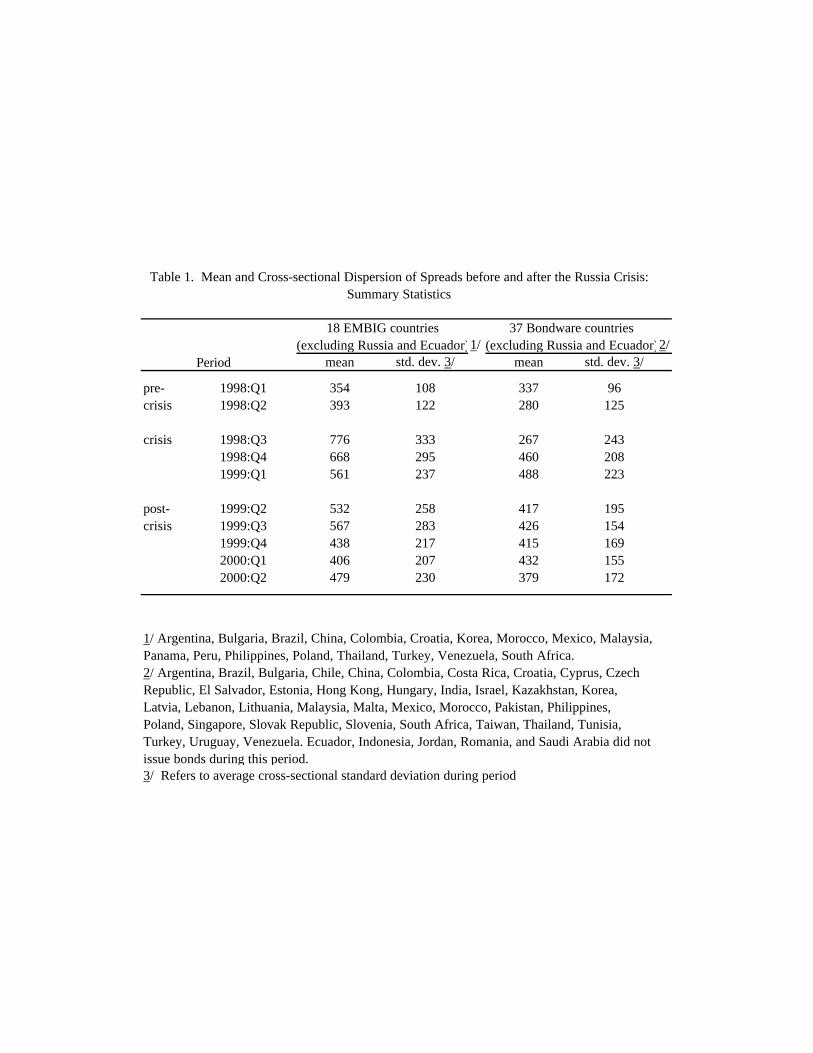
1/ 2/mean std. dev. 3/ mean std. dev. 3/

pre- 1998:Q1 354 108 337 96crisis 1998:Q2 393 122 280 125

crisis 1998:Q3 776 333 267 2431998:Q4 668 295 460 2081999:Q1 561 237 488 223

post- 1999:Q2 532 258 417 195crisis 1999:Q3 567 283 426 154

1999:Q4 438 217 415 1692000:Q1 406 207 432 1552000:Q2 479 230 379 172

2/ Argentina, Brazil, Bulgaria, Chile, China, Colombia, Costa Rica, Croatia, Cyprus, Czech Republic, El Salvador, Estonia, Hong Kong, Hungary, India, Israel, Kazakhstan, Korea, Latvia, Lebanon, Lithuania, Malaysia, Malta, Mexico, Morocco, Pakistan, Philippines, Poland, Singapore, Slovak Republic, Slovenia, South Africa, Taiwan, Thailand, Tunisia, Turkey, Uruguay, Venezuela. Ecuador, Indonesia, Jordan, Romania, and Saudi Arabia did not issue bonds during this period.

18 EMBIG countries

3/ Refers to average cross-sectional standard deviation during period

Table 1. Mean and Cross-sectional Dispersion of Spreads before and after the Russia Crisis: Summary Statistics

37 Bondware countries(excluding Russia and Ecuador)(excluding Russia and Ecuador)

Period

1/ Argentina, Bulgaria, Brazil, China, Colombia, Croatia, Korea, Morocco, Mexico, Malaysia, Panama, Peru, Philippines, Poland, Thailand, Turkey, Venezuela, South Africa.

Test for Test for Test for equality equality equality

Variable Coef. p Coef. p p 4/ Coef. p Coef. p p 4/ Coef. p Coef. p p 4/

Constant 27190.79 0.43 1177.15 0.00 0.45 3461.78 0.23 815.35 0.00 0.36 2583.30 0.35 881.40 0.00 0.54

Real growth (MA) 26.04 0.23 -44.64 0.00 0.00 33.82 0.16 -43.52 0.00 0.00 20.42 0.89 -110.25 0.00 0.38

(Real growth)2 0.41 0.98 2.36 0.20 0.89Inflation 1.28 0.28 0.50 0.56 0.60Current account (MA) -1.08 0.76 -4.73 0.02 0.36Total Debt/GDP -0.05 0.98 -0.90 0.00 0.64Brady dummy 74.39 0.23 60.38 0.07 0.82 63.54 0.35 60.94 0.04 0.97 56.23 0.71 207.81 0.00 0.35Rating (residual) -27.95 0.01 -62.46 0.00 0.00 -24.36 0.10 -66.33 0.00 0.01 -25.03 0.67 -127.20 0.00 0.12(rating residual)² -0.01 1.00 3.66 0.00 0.23

LIBOR -593.06 0.24 -58.85 0.01 0.29 -428.46 0.37 -98.61 0.00 0.49US ten year yield -4847.57 0.44 -111.27 0.00 0.45

F test (p) 0.00 0.00 0.00No. quarters 86No. bond quarters 19No. countries 5/ 43

Coef. Coef. Coef.

Debt issued in preceding year -0.12 -0.20 -0.61Number of issues preceding 0.17 0.19 0.18GDP per capita (1993) 0.19 0.22 0.15dummy for Asian crisis countries -0.13 -0.26 -0.23

rho 0.17 -0.08 -0.09

1/ Estimated on pooled sample 1998:Q1 - 2000:Q2, excluding 1998:Q3 - 1999:Q1, and allowing for different coefficients for pre- and post crisis periods2/ 1998:Q1 - 1998:Q23/ 1999:Q1 - 2000:Q24/ p values based on two-sided tests; boldface indicates rejection of equality at the 5 percent level in the direction consistent with H1 (see text).

6/ Reports only coefficients for instruments and correlation coefficient of disturbance terms of the two equations (rho).

before crisis 2/ after crisis 3/

215

Selection Equation 6/

before crisis 2/ after crisis 3/ before crisis 2/

0.800.64 0.78

0.48

84 210

0.420.00

0.790.000.38

4319 84

0.52

42 4243 43

Table 2. Launch Spread Data: Estimation of Alternative Models Before and After Russian Crisis, and Results for "Coefficients Test"

(1) "Eichengreen-Mody" 1/

19 8686 215

86

(2) Alternative specification 1/ (3) Alternative including squares 1/

after crisis 3/

pp

5/ Argentina, Brazil, Bulgaria, Chile, China, Colombia, Costa Rica, Croatia, Cyprus, Czech Republic, Ecuador, El Salvador, Estonia, Hong Kong, Hungary, India, Indonesia, Israel, Jordan, Kazakhstan, Korea, Latvia, Lebanon, Lithuania, Malaysia, Malta, Mauritius, Mexico, Pakistan, Philippines, Poland, Romania, Saudi Arabia, Singapore, Slovak Republic, Slovenia, South Africa, Taiwan, Thailand, Tunisia, Turkey, Uruguay, Venezuela. Model (2) excludes El Salvador.

p

0.860.000.380.66 0.41

Argentina 2 0 3 0 1 0Brazil 2 0 4 0 4 0Bulgaria 2 0 5 0 0 0Chile 0 0 0 2 0 0China 0 0 0 2 0 0Colombia 2 0 2 0 0 0Costa Rica 2 0 2 0 1 0Croatia 2 0 1 0 1 0Cyprus 0 0 0 0 0 0Czech Republic 0 0 0 0 0 0Ecuador 2 0 4 0 3 0El Salvador 2 0 ... ... 0 0Estonia 0 0 0 0 0 0Hong Kong 0 0 0 0 0 0Hungary 2 0 2 0 1 0India 0 0 0 0 0 0Indonesia 1 0 3 0 2 0Israel 0 0 0 0 0 0Jordan 2 0 4 0 2 0Kazakhstan 2 0 3 0 4 0Korea 0 0 0 0 0 0Latvia 2 0 1 0 0 0Lebanon 2 0 0 0 3 0Lithuania 2 0 2 0 0 0Malaysia 0 0 0 2 0 0Malta 0 0 0 0 0 0Mauritius 0 0 0 0 0 0Mexico 2 0 2 0 2 0Pakistan 2 0 4 0 5 0Philippines 0 0 0 0 0 0Poland 0 0 0 0 0 0Romania 2 0 5 0 2 0Saudi Arabia 2 0 4 0 0 0Singapore 0 0 0 2 0 0Slovak Republic 0 0 0 0 0 0Slovenia 0 0 0 0 0 0South Africa 2 0 3 0 1 0Taiwan Province of China 0 0 0 2 0 0Thailand 0 0 2 0 0 0Tunisia 1 0 1 0 0 0Turkey 2 0 0 0 3 0Uruguay 1 0 0 0 0 0Venezuela 2 0 5 0 3 0

Sum rejections 45 0 62 10 38 0... out of total: 3/ 254 47 202 92 222 79

No. countries showing rejection 4/ 24 0 21 5 16 0Total no. of countries

Rejections indicating ... Rejections indicating ... Rejections indicating ...

43 42 43

Table 3. Launch Spread Data: Summary Results for "Levels Test" (Russia Crisis)

Eichengreen-Mody: Alternative model: Alternative incl. squares

4/ No. of countries showing several periods with significant change in spreads in one direction and no more than one period showing a significant change in opposite direction.

3/ Total number of periods in which fitted spread based on post-crisis model is higher than fitted spread based on pre-crisis model (left columns) or vice versa (right columns), regardless of significance.

significant increase of spreads 1/

significant decline of spreads 2/

1/ No. of periods in which fitted spread based on post-crisis model is significantly higher than fitted spread based on pre-crisis model (potential maximum: 7).2/ No. of periods in which fitted spread based on post-crisis model is significantly lower than fitted spread based on pre-crisis model (potential maximum: 7).

significant increase of spreads 1/

significant decline of spreads 2/

significant increase of spreads 1/

significant decline of spreads 2/

Test for Test for Test forequality equality equality

before after before after before afterQuarter crisis 1/ crisis 2/ (p ) 3/ crisis 1/ crisis 2/ (p ) 3/ crisis 1/ crisis 2/ (p ) 3/

1998:Q1 10107 34704 0.017 9761 33942 0.009 8568 27933 0.0141998:Q2 10547 35692 0.017 11149 37021 0.008 8952 30532 0.008

1999:Q2 8330 43921 0.000 9568 46481 0.000 8180 47922 0.0001999:Q3 8317 43909 0.000 9541 46894 0.000 8198 48008 0.0001999:Q4 8455 45844 0.000 9550 48917 0.000 8261 51102 0.0002000:Q1 7344 46706 0.000 8266 47994 0.000 6852 52017 0.0012000:Q2 7301 48657 0.000 8155 50440 0.000 6809 56007 0.000

Table 4. Launch Spread Data: Cross-sectional Variances of Fitted Spreads before and after Russian Crisis, and Results for "Variance Test"

(1) Eichengreen-Mody (2) Alternative specification (3) Alternative including squares

2/ Regression coefficients estimated on the basis of post-crisis data (see Table 2).

Fitted variance using coefficients estimated

Fitted variance using coefficients estimated

Fitted variance using coefficients estimated

1/ Regression coefficients estimated on the basis of pre-crisis data (see Table 2).

Test for Test for Test for equality equality equality

Variable Coef. p Coef. p p 4/ Coef. p Coef. p p 4/ Coef. p Coef. p p 4/Constant 1051.16 0.28 1405.95 0.00 0.73 932.99 0.33 1450.96 0.00 0.60 1904.13 0.00 2399.78 0.00 0.30

Real growth -11.01 0.00 -3.36 0.03 0.00 -10.78 0.00 -1.48 0.52 0.00 -5.06 0.00 -18.03 0.00 0.00Inflation 0.52 0.00 -1.17 0.07 0.01Fiscal balance 12.93 0.00 25.45 0.00 0.03Current account (MA) 13.53 0.00 24.95 0.00 0.05 8.53 0.03 32.56 0.00 0.00Growth of the Real Exchange Rate -0.23 0.62 -5.43 0.00 0.00Relative price of non-fuel, non-manufacturing goods -1146.30 0.00 -1650.88 0.00 0.28Reserves/Short Term Debt -0.14 0.00 -0.11 0.11 0.75 -0.34 0.00 -0.39 0.00 0.60Total Debt/Exports 0.00 0.00 0.00 0.52 0.00Total Debt/GDP -0.51 0.0 -0.74 0.00 0.02Short Term Debt/Total Debt -2.30 0.00 -6.45 0.00 0.00Brady dummy 75.53 0.00 227.09 0.00 0.00Arrears dummy 61.29 0.00 267.24 0.00 0.00 35.28 0.00 190.14 0.00 0.00Rating (residual) -37.81 0.00 -63.43 0.00 0.00 -32.00 0.00 -58.01 0.00 0.00 -56.23 0.00 -75.07 0.00 0.02Real credit growth (MA) -2.04 0.01 -2.24 0.04 0.88Political Instability and Violence -59.68 0.00 -183.70 0.00 0.00Asia dummy -30.78 0.09 -207.42 0.00 0.00 -15.58 0.42 -230.88 0.00 0.00Latin dummy 115.49 0.00 249.77 0.00 0.00 103.17 0.00 233.67 0.00 0.00

US ten year yield -199.63 0.16 -132.90 0.00 0.65 -180.31 0.19 -131.44 0.00 0.73US high-yield bond spread 142.36 0.03 -31.11 0.51 0.03 154.57 0.01 -27.94 0.55 0.02log of US$ GDP -8.14 0.06 5.54 0.40 0.09

F-test (p ) 0.00 0.00 0.00NNo. countries 4/kR Sq.

1/ Estimated on pooled sample allowing for different coefficients for pre- and post crisis periods2/ January 1998 to July 1998, using monthly data3/ April 1999 to December 1999, using monthly data4/ p values based on two-sided tests; boldface indicates rejection of equality at the 5 percent level in the direction consistent with H1 (see text).

10 100.810.74

124 16218 18

0.82 0.89

124 16218 1811 11

0.77 0.82

after crisis 3/

14141818162124

Table 5. EMBIG Data: Estimation of Alternative Models Before and After Russia Crisis, and Results for "Coefficients Test"

5/ Full sample of 18 countries: Argentina, Bulgaria, Brazil, China, Colombia, Croatia, Korea, Morocco, Mexico, Malaysia, Panama, Peru, Philippines, Poland, Thailand, Turkey, Venezuela, South Africa.

(1) "Eichengreen-Mody" 1/ (2) Alternative specification (A) 1/ (2) Alternative specification (B) 1/

before crisis 2/ after crisis 3/ before crisis 2/ after crisis 3/ before crisis 2/

Argentina 7 0 7 0 0 7Brazil 7 0 7 0 9 0Bulgaria 10 0 9 0 9 4China 0 2 0 2 0 16Colombia 7 0 7 0 2 0Croatia 7 0 7 0 3 5Korea 0 7 0 7 1 9Malaysia 0 7 0 8 0 15Mexico 7 0 7 0 2 0Morocco 0 0 3 0 0 4Panama 7 0 7 0 0 0Peru 7 0 7 0 0 5Philippines 0 2 0 4 0 9Poland 5 0 7 0 0 12South Africa 3 0 5 0 0 13Thailand 0 7 0 8 0 9Turkey 7 0 5 0 0 7Venezuela 7 0 7 0 10 0

Sum rejections 81 25 85 29 36 115... out of total: 3/ 200 88 177 111 104 184

No. countries showing rejection 4/ 12 5 13 5 4 12Total no. of countries

4/ No. of countries showing several periods with significant change in spreads in one direction and no more than one period showing a significant change in opposite direction.

3/ Total number of periods in which fitted spread based on post-crisis model is higher than fitted spread based on pre-crisis model (left columns) or vice versa (right columns), regardless of significance.

1/ No. of periods in which fitted spread based on post-crisis model is significantly higher than fitted spread based on pre-crisis model (potential maximum: 16).2/ No. of periods in which fitted spread based on post-crisis model is significantly lower than fitted spread based on pre-crisis model (potential maximum: 16).

Table 6. EMBIG Data: Summary Results for "Levels Test"

significant increase of spreads 1/

significant increase of spreads 1/

significant decline of spreads 2/

significant decline of spreads 2/

Alternative model B:Alternative model A:Eichengreen-Mody

significant increase of spreads 1/

significant decline of spreads 2/

Rrejections indicating ... Rejections indicating ... Rejections indicating ...

18 18 18

Test for Test for Test forequality equality equality

before after before after before afterMonth crisis 1/ crisis 2/ (p ) 3/ crisis 1/ crisis 2/ (p ) 3/ crisis 1/ crisis 2/ (p ) 3/

1998:01 14474 11438 64210 0.000 12520 90302 0.006 15233 36846 0.0001998:02 11714 11340 65771 0.000 12002 67257 0.000 14663 33563 0.0001998:03 8909 10782 62403 0.000 11123 63492 0.000 13523 33311 0.0001998:04 10099 10329 60648 0.000 10714 62593 0.000 11517 32243 0.0001998:05 14559 10329 60648 0.000 10716 62427 0.000 11665 33415 0.0001998:06 20586 10329 60648 0.000 10710 62707 0.000 11879 34562 0.0001998:07 23638 9356 56498 0.000 9148 59008 0.000 11095 40041 0.000

1999:04 53108 9449 53503 0.000 9846 53393 0.000 12056 53903 0.0001999:05 80188 9449 53503 0.000 9841 53609 0.000 12240 53166 0.0001999:06 67609 9748 54126 0.000 10160 54180 0.000 12784 57795 0.0001999:07 78276 9349 52807 0.000 10111 54511 0.000 12633 58504 0.0001999:08 95792 9309 52639 0.000 10035 53882 0.000 12011 57081 0.0001999:09 66819 10106 54630 0.000 10755 55624 0.000 13041 59801 0.0001999:10 50033 10248 55428 0.000 10878 56755 0.000 13699 62338 0.0001999:11 52809 10273 56507 0.000 10824 57604 0.000 14149 65678 0.0001999:12 38487 10710 58895 0.000 11168 59702 0.000 15159 66471 0.000

3/ Regression coefficients estimated on 1999:03 to 1999:12 data.2/ Regression coefficients estimated on 1998:01 to 1998:07 data.

Actual Variance 1/

(1) Eichengreen-Mody (2) Alternative specification (A)Fitted variance using coefficients estimated

Fitted variance using coefficients estimated

Fitted variance using coefficients estimated ...

(2) Alternative specification (B)

Table 7. EMBIG Data: Cross-sectional Variances of Fitted Spreads before and after Russian Crisis, and Results for "Variance Test"

1/ Sample of 18 countries excluding Russia and Ecuador (see Table 5)

Test for Test for equality equality

Variable Coef. p Coef. p p 6/ Coef. p Coef. p p 6/

Constant 203.1 0.06 387.9 0.07 0.44 841.0 0.01 5650.7 0.01 0.02

Real growth (MA) -15.91 0.00 -6.38 0.02 0.05 -10.78 0.00 69.31 0.00 0.00Inflation 39.51 0.09 171.46 0.00 0.01 184.38 0.00 257.88 0.04 0.57Current account (MA) -0.84 0.56 0.42 0.70 0.49 -2.30 0.14 -12.52 0.14 0.23Brady dummy 32.29 0.40 164.34 0.00 0.00 88.91 0.00 50.66 0.28 0.44Rating (residual) -18.06 0.01 -16.88 0.00 0.88 -18.57 0.00 -20.01 0.04 0.89

LIBOR 7.37 0.74 -43.27 0.25 0.25 -112.59 0.06 -1004.3 0.01 0.02

F test (p) 0.01 0.00No. quartersNo. bond quartersNo. countries 7/

Coef. Coef.

Debt issued in preceding year -3.99 -3.15Number of issues preceding 0.20 0.19GDP per capita (1993) -0.06 -0.02dummy for Asian crisis countries -0.75

rho -0.24 -0.69

2/ 1994:Q1 - 1994:Q33/ 1995:Q3 - 1997:Q24/ 1996:Q1 - 1997:Q25/ 1998:Q1 - 1998:Q2

8/ Reports only coefficients for instruments and correlation coefficient of disturbance terms of the two equations (rho).

1/ Using model (2) of Table 2 in both cases. Regression (1) is based on the sample 1994:Q1 - 1997:Q2, regression (2) on the sample 1996:Q1 - 1998:Q2.

69 18425 10423 23

0.040.000.79

p

33 33

0.24

0.020.000.91

198 6690 17

Table A1. Launch Spread Data: Estimation Results Before and After the Mexican and Asian Crises,

(1) Mexican Crisis

0.00

and "Coefficients Test" 1/

0.26

(2) Asian Crisis

Selection Equation 8/

before crisis 2/ after crisis 3/ before crisis 4/ after crisis 5/

6/ p values based on two-sided tests; boldface indicates rejection of equality at the 5 percent level in the direction consistent with H1 (see text).

Korea, Malaysia, Malta, Mexico, Philippines, Singapore, Taiwan, Thailand, Trinidad and Tobago, Turkey, Uruguay, Venezuela. Sample in model (2): Argentina, Brazil, Chile, China, Colombia, Cyprus, Czech Republic, Hong Kong, Hungary, India, Indonesia, Israel, Jordan, Korea, Malaysia, Malta, Mauritius, Mexico, Pakistan, Philippines, Poland, Romania, Saudi Arabia, Singapore, Slovak Republic, South Africa, Taiwan, Thailand, Trinidad and Tobago, Tunisia, Turkey, Uruguay, Venezuela.

7/ Sample in model (1): Argentina, Brazil, Chile, China, Colombia, Cyprus, Hong Kong, Hungary, India, Indonesia, Israel,

p

Argentina 3 0 5 0Brazil 4 0 2 0Chile 0 0 8 0China 0 0 8 0Colombia 0 0 6 0Cyprus 0 0 4 0Czech Republic ... ... 5 0Hong Kong 0 0 1 0Hungary 0 2 0 1India 0 0 8 0Indonesia 0 0 8 0Israel 0 0 8 0Jordan ... ... 5 0Korea 0 0 8 0Malaysia 0 0 8 0Malta 0 0 7 0Mauritius ... ... 6 0Mexico 4 0 0 2Pakistan ... ... 5 0Philippines 0 0 2 0Poland ... ... 7 0Romania ... ... 1 0Saudi Arabia ... ... 0 2Singapore 0 0 5 0Slovak Republic ... ... 3 0South Africa ... ... 0 0Taiwan 0 0 6 0Thailand 0 0 8 0Trinidad and Tobago 0 3 0 0Tunisia ... ... 6 0Turkey 0 0 6 0Uruguay 9 0 3 1Venezuela. 10 0 0 2

Sum rejections 30 5 149 8... out of total: 4/ 128 125 216 48

No. countries showing rejection 5/ 5 2 27 5Total no. of countries

1/ Using models presented in Table A1.

5/ No. of countries showing several periods with sig. change in spreads in one direction and no more than one period with sig. change in opposite direction.

significant increase of spreads 2/

significant decline of spreads 3/

2/ Periods in which fitted spread based on post-crisis model is significantly higher than fitted spread based on pre-crisis model (potential maximum: 7).3/ Periods in which fitted spread based on post-crisis model is significantly lower than fitted spread based on pre-crisis model (potential maximum: 7).

significant increase of spreads 2/

significant decline of spreads 3/

4/ Total no. of periods in which fitted spread based on post-crisis model is higher than fitted spread based on pre-crisis model (left columns) or vice versa (right columns),regardless of significance.

23 33

Rejections indicating ... Rejections indicating ...

Table A2. Launch Spread Data: Summary Results for "Levels Test",

Mexican Crisis Asian Crisis

Mexican and Asian Crises 1/

Test for Test forequality equality

before after before afterQuarter crisis 1/ crisis 2/ (p ) 3/ crisis 1/ crisis 2/ (p ) 3/

1994:Q1 6044 27609 0.0211994:Q2 6300 30873 0.0261994:Q3 6462 31550 0.026

1995:Q3 6178 12162 0.0491995:Q4 6006 12118 0.0391996:Q1 5969 12357 0.032 7244 38819 0.1201996:Q2 5987 12490 0.030 7206 39032 0.1191996:Q3 6005 12666 0.028 7260 38733 0.1201996:Q4 5937 12584 0.027 7264 38736 0.1181997:Q1 5741 12550 0.024 7317 27017 0.1581997:Q2 5592 11657 0.036 7185 27756 0.157

1998:Q1 6213 20860 0.1191998:Q2 6239 21973 0.108

2/ Regression coefficients estimated on the basis of post-crisis data (see Table A1).3/ p values based on two-sided tests.

Fitted variance using coefficients estimated ...

Fitted variance using coefficients estimated ...

1/ Regression coefficients estimated on the basis of pre-crisis data (see Table A1).

Table A3. Launch Spread Data: Cross-sectional Variances of Fitted Spreads beforeand after Mexican and Asian Crises, and Results for "Variance Test"

(1) Mexican Crisis (2) Asian Crisis

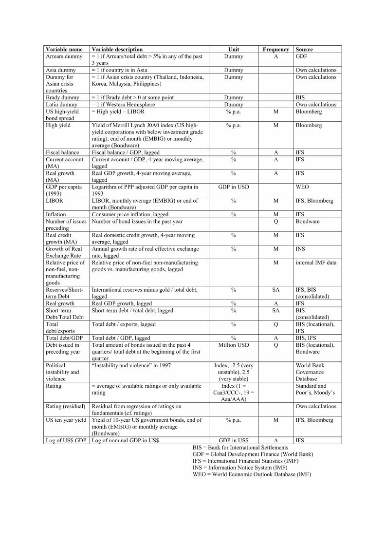
Variable name Variable description Unit Frequency SourceArrears dummy = 1 if Arrears/total debt > 5% in any of the past

3 yearsDummy A GDF

Asia dummy = 1 if country is in Asia Dummy Own calculationsDummy forAsian crisiscountries

= 1 if Asian crisis country (Thailand, Indonesia,Korea, Malaysia, Philippines)

Dummy Own calculations

Brady dummy = 1 if Brady debt > 0 at some point Dummy BISLatin dummy = 1 if Western Hemisphere Dummy Own calculationsUS high-yieldbond spread

= High yield � LIBOR % p.a. M Bloomberg

High yield Yield of Merrill Lynch J0A0 index (US high-yield corporations with below investment graderating), end of month (EMBIG) or monthlyaverage (Bondware)

% p.a. M Bloomberg

Fiscal balance Fiscal balance / GDP, lagged % A IFSCurrent account(MA)

Current account / GDP, 4-year moving average,lagged

% A IFS

Real growth(MA)

Real GDP growth, 4-year moving average,lagged

% A IFS

GDP per capita(1993)

Logarithm of PPP adjusted GDP per capita in1993

GDP in USD WEO

LIBOR LIBOR, monthly average (EMBIG) or end ofmonth (Bondware)

% M IFS, Bloomberg

Inflation Consumer price inflation, lagged % M IFSNumber of issuespreceding

Number of bond issues in the past year Q Bondware

Real creditgrowth (MA)

Real domestic credit growth, 4-year movingaverage, lagged

% M IFS

Growth of RealExchange Rate

Annual growth rate of real effective exchangerate, lagged

% M INS

Relative price ofnon-fuel, non-manufacturinggoods

Relative price of non-fuel non-manufacturinggoods vs. manufacturing goods, lagged

M internal IMF data

Reserves/Short-term Debt

International reserves minus gold / total debt,lagged

% SA IFS, BIS(consolidated)

Real growth Real GDP growth, lagged % A IFSShort-termDebt/Total Debt

Short-term debt / total debt, lagged % SA BIS(consolidated)

Totaldebt/exports

Total debt / exports, lagged % Q BIS (locational),IFS

Total debt/GDP Total debt / GDP, lagged % A BIS, IFSDebt issued inpreceding year

Total amount of bonds issued in the past 4quarters/ total debt at the beginning of the firstquarter

Million USD Q BIS (locational),Bondware

Politicalinstability andviolence

�Instability and violence� in 1997 Index, -2.5 (veryunstable), 2.5(very stable)

World BankGovernanceDatabase

Rating = average of available ratings or only availablerating

Index (1 =Caa3/CCC-, 19 =

Aaa/AAA)

Standard andPoor�s, Moody�s

Rating (residual) Residual from regression of ratings onfundamentals (cf. ratings)

Own calculations

US ten year yield Yield of 10-year US government bonds, end ofmonth (EMBIG) or monthly average(Bondware)

% p.a. M IFS, Bloomberg

Log of US$ GDP Log of nominal GDP in US$ GDP in US$ A IFSBIS = Bank for International SettlementsGDF = Global Development Finance (World Bank)IFS = International Financial Statistics (IMF)INS = Information Notice System (IMF)WEO = World Economic Outlook Database (IMF)