monte carlo tree search in go - university of albertammueller/ps/2013/2013-gochapter... · monte...
TRANSCRIPT

Monte Carlo Tree Search in Go
Adrien Couetoux and Martin Muller and Olivier Teytaud
Abstract Monte Carlo Tree Search (MCTS) was born in Computer Go, i.e. in theapplication of artificial intelligence to the game of Go. Since its creation, in 2006,many improvements have been published. Programs are still by far weaker thanthe best human players, yet the gap was very significantly reduced. MCTS is nowwidely applied in games, in particular when no trustable evaluation function is read-ily available. This chapter reviews the development of current strong Go programsand the most important extensions to MCTS that are used in this game.
1 Introduction
This chapter describes the application of Monte Carlo Tree Search (MCTS) meth-ods to the game of Go. Computer Go was the first major success story for MCTS,and many important techniques were developed in this context. Go remains the beststudied application, with a huge amount of practical work as well as many publica-tions over the last seven years.
The game of Go is a perfect information turn-based two player board game. Asusual in board games, actions are called moves. In Go, a normal move consists inplacing a single stone on the Go board, plus removing any captured opponent stonesfrom the board. Special move types are passing and resigning.
Adrien CouetouxInstitute of Information Science, Academia Sinica, Taiwan, e-mail: [email protected]
Martin MullerDepartment of Computing Science, University of Alberta, Canada, e-mail: [email protected]
Olivier Teytaud, Tao, Inria, Lri, UMR CNRS 8623, Universite Paris-Sud, France e-mail:[email protected]
1

2 Adrien Couetoux and Martin Muller and Olivier Teytaud
The state of a Go game is described by the location of black and white stoneson the board, plus the move history, including who plays next. History is needed tocheck the Ko rules which forbid certain types of repetition (see Section 1.2). Someversions of the rules also require keeping track of the number of captured stones.
Notation: Throughout the chapter, moves are denoted by m, states by s, and theplayer to play in state s by player(s).
1.1 The importance of Go
The game of Go originated in China more than 2000 years ago. It has simple rules,but advanced tactics and a striking strategic level. It is the oldest known abstractboard game, and is actively played by millions of people. There is a large commu-nity of hundreds of professional Go players, mainly in Asia. These players study,teach and play Go full-time. Compared to many other classical games, progress inComputer Go has been much slower, and it has been considered a “grand challenge”of artificial intelligence. The recent breakthrough of MCTS has, for the first time,led to strong computer programs, and has even opened up perspectives to approachthe level of the best human professionals. This level has already been achieved onsmall boards of size 9×9 and smaller.
A key feature about Go is its great strategic depth. The depth of a game [53]is defined as the maximum number of players p1, . . . , pdepth such that, if 1 ≤ j <i ≤ depth, player p j wins with probability at least 60% against pi . Depth is notalways clearly defined, and it relies on a set of players, but it makes it possible tocompare different games. Go has a depth around 40, which is much more than anyother known game.
1.2 The rules of Go
Go is played by placing stones on the intersections of a square board. The standardboard size is 19× 19, but smaller sizes are popular for teaching and quick games.Black plays first, then the two players (black and white) alternate until the gameends with two or three consecutive passes, or with a resignation. Stones never moveon the board, but are removed when captured. Examples and details of these rulesare given in Fig. 1. The Ko rule prevents players from creating a potentially endlessloop by repeating a previous situation. This rule is explained in Fig. 2. At the end,the player with the larger score is the winner. The exact scoring method dependson the rules used. The simplest method used by most Go programs is a variant ofChinese rules, which counts both stones and surrounded empty points, called terri-tories, for each player (see Fig. 3). The score can be adjusted by a fixed value calledKomi. This is used to compensate for the advantage of the first player, or sometimesto compensate for the different strength of the players. The more usual method to

Monte Carlo Tree Search in Go 3
Fig. 1 Rules of the game of Go.Blocks: A block of stones is a maximal 4-connected set of stones of the same color. For exam-ple, {J7,J8,J9} is a block, but {J7,J8} is not (not maximal) and {J7,J8,J9,K6} is also not (not4-connected). A block of stones can be referred to by any of its stones: block J7 is the same as theblock J8.Liberties: The empty intersections adjacent to a block are called its liberties. For example, blockA1 has a single liberty at C2, while block A2 has three liberties at A3, B3 and C2.Capture: A block of stones is captured if the opponent fills its last liberty. For example, Black C2captures the White block {A1,B1,C1,D1,E1,F1}. Captured stones are removed and these intersec-tions become empty again. It is possible to capture several blocks in one move. For example, BlackC8 captures the two white blocks A6 and A9.Suicide: In most variations of the Go rules, it is illegal to play a stone that fills the last liberty of theplayer’s own block, while not capturing any opponent. For example, White L8 is suicide whereasBlack L8 is a capture and is allowed. White A8 is also suicide. White can play either one of E15or G15 but not both. Black can not play either move. T17 is the last liberty of both the white blockT18, and the black block T16. Whoever plays first can capture the other.Chains, groups etc: Closely related or virtually connected sets of blocks are often called chainsor groups. The notation is not consistent in the literature. Typically, a group is treated as a unit andall its blocks are expected to live together or die together. Cutting off a group from other blocks isconsidered an important event in a game.
compensate strength differences is to give handicap stones: Black is allowed to makeseveral consecutive moves at the start of the game.
For more information about the game of Go in general, see [8, 68]. For informa-tion about rules and variations, see [69].
Two important Go concepts are eyes, and the safety of blocks of stones. GroupE16 in Fig. 1 has two eyes at E15 and G15. Playing either of these moves would besuicide for Black (cf Fig. 1). Therefore, a group with two eyes can not be killed by

4 Adrien Couetoux and Martin Muller and Olivier Teytaud
Fig. 2 The Ko rule: In the figure on the left-hand side, white can capture a single stone with D4,leading to the position on the right. The Ko rule forbids Black from immediately recapturing onE4 which would repeat the position on the left. All Ko rules prevent such simple cycles of length2. Rules differ in their handling of longer, more complex cycles [69].
the opponent; it is safe unless its owner fills its own eyes. In contrast, block K7 hasonly one eye; it can be killed by Black L8.
Computational Complexity.
A variant of the rules, namely the Japanese rules, is known to be Exptime-hard [54];more precisely, this (not fully defined) set of rules contains a well defined set ofpositions which is Exptime-complete. The Chinese variant is completely definedbut its complexity is unknown; it is in the (huge) gap between Pspace-hard [22] andExpspace.
1.3 Computer Go before Monte Carlo Tree Search
Work on Computer Go started fifty years ago. Early programs were rule-based sys-tems, and dealt with basic tactics such as ladders. The advent of affordable personalcomputers in the mid 1980’s led to a big boost in popularity, and to the creation ofthe first regular tournaments such as the Ing cup.
Wilcox describes the early development of Computer Go up to the late 1970’s[70]. The first large-scale Go program was Interim.2, written in Lisp by Reitmanand Wilcox [51]. Reviews of the development of Computer Go up to about the year2000 and detailed survey papers covering “classical” Computer Go were publishedabout ten years ago [6, 45, 46].

Monte Carlo Tree Search in Go 5
Fig. 3 Scoring: When no player is willing to keep playing (both play a pass) the game is stoppedand we count who has won. E.g. for Chinese rules, the points for Black are (i) the black stoneson the board (ii) the areas enclosed by black stones. The points for White are (i) the white stoneson the board (ii) the areas enclosed by white stones (iii) a bonus for White, termed Komi, e.g.5.5, aimed at compensating Black’s advantage of first play. Here, on a 7×7 board, Black has 21,whereas White has 28+5.5 = 33.5; White has won by 12.5 points. Players can play until they seethat whatever additional stone they play, it will be captured; at some point there will be no morelegal move. The game is usually stopped far before there is no legal move.
One measure of progress were the yearly handicap exhibition matches betweenthe Ing Cup winner and three young human players, often of insei (student profes-sional) strength. The strength of the computer program would then be measured byhow many stones it needed to win (the less stones, the better the program). The firsthurdle at 17 stones handicap was taken in 1991 by Mark Boon’s program GOLIATH.In 1997, Chen Zhixing’s HANDTALK won on 11 stones. At the time of the last IngCup in 2000, programs had not yet won a game at 9 stones, which is consideredthe highest handicap in regular use. Nick Wedd maintains a website with detailedinformation, including game records, of all man-machine Go matches [67].
Progress was slow. As computers got faster, programs started to use morespecialized tactical searches such as block capture and life and death. GOLIATHimplemented a successful goal-oriented global search. Other programs such asHANDTALK, THE MANY FACES OF GO and GO++ also started using global search.The main obstacle for progress with using traditional alpha-beta based methods inGo was the lack of a fast but reasonable evaluation function.
One notable development of the years leading up to the Monte Carlo revolutionwas the rise of GNU GO, the first strong open source Go program [28].
Typical ingredients of a “classical”, pre-Monte Carlo Go program were:

6 Adrien Couetoux and Martin Muller and Olivier Teytaud
• A fast implementation of a Go board, including rules, executing and taking backmoves, blocks and their liberties
• A ladder reading module, sometimes implemented on a specialized board withreduced “lazy” updates
• An influence function which radiates out from stones, and allows the program toassign a “likely owner” to each empty point
• A pattern matching system, typically containing several thousand hand-made pat-terns, with extra attributes such as liberty counts
• A sophisticated set of data structures for higher-level units on a Go board, suchas chains, groups, and territories
• A set of heuristics for recognizing and evaluating eyes and potential eyes• Specialized selective search modules for capturing blocks of stones, and for life
and death of groups• A highly selective, shallow global search• An opening book containing standard joseki corner sequences
Since the overall problem of playing Go well appeared intractable, quite a bit ofwork has gone into specialized approaches to handle specific subproblems of Go.Representative examples are life and death solvers [71, 39], specialized searchesfor capturing blocks of stones [63], solving endgame puzzles using methods fromcombinatorial game theory [44], proving the safety of stones and territories [4, 43,49, 50], and solving seki [48].
Van der Werf has solved Go for several small but highly nontrivial board sizesincluding 5× 5 [64], 5× 6 and 4× 7 [65]. An overview table is shown on http://erikvanderwerf.tengen.nl/mxngo.html.
Towards MCTS for Go
While the top-level structure of MCTS-based Go programs is completely differentfrom classical ones, some components have been kept, reintroduced, or further re-fined:
• Fast incremental data structures for maintaining a board, blocks and liberties• Tools for dealing with large numbers of game records from master players or
from computer players; tools for automated testing and parameter tuning usingself-play and tournaments
• Zobrist hashing [74]: the Zobrist hash is a fast and fair method for mappingfrom Go boards to integers. It is used for storing positions in transposition tables.This can save memory and computational cost by avoiding duplicates in the tree.However, dealing with the resulting cyclic and acyclic graphs in MCTS has itsown challenges [16, 55].
• The AMAF and RAVE methods described in Section 3.1 are related to, but dif-ferent from the history heuristic [56] used in alphabeta search.
• Heuristic Go knowledge in the form of pattern matching (Section 3.2), expertrules (Section 3.3), and opening books (Section 3.4).
Monte Carlo Tree Search in Go 7
There are also approaches based on reinforcement learning. NeuroGo [25] usesreinforcement learning (Section 1.5) with neural networks, and RLGO [60] usesboth offline and online learning of weights for patterns up to size 3×3.
Bernd Bruegmann designed the first Go evaluation function using Monte Carlosimulations and implemented it in his Gobble program [10]. His approach simulatesmany random games from a given state, and estimates the move values by theirwinning probability. This algorithm missed the crucial second component of MCTS,the tree search, and its performance was much weaker than the classical programsat the time. Therefore, there was little follow-up work for several years.
1.4 The Bandit Literature
In this section, we introduce the bandit literature, which is a theoretical, maybe morethan practical, ground for MCTS. Developed during the recent decades, this body ofwork is devoted to the problem of choosing one action a in a set of K options (alsotermed arms), at each time step t ∈ {1, . . . ,T}. One obtains a stochastic reward eachtime an action is selected. Some of the common objectives are to maximize the ex-pected total reward from 1 to T , or to maximize the expected reward obtained at thelast time step. In the former case, one needs to balance exploration and exploita-tion. Focusing on exploration only would mean to choose actions uniformly in orderto explore as many options as possible, to avoid missing a good one. On the otherhand, focusing on exploitation would mean choosing the action that has the bestempirical average reward. This balance is at the heart of successful approaches tomulti-armed bandit problems.
In the case of Monte Carlo Tree Search, bandit algorithms are used for choosingwhich moves should be simulated more often in a given state (Section 2). The goal isto balance the exploration of actions that we know little about versus the exploitationof actions that returned the highest rewards in the past (the incentive being that wemay want to simulate these promising moves to confirm their high value).
The bandit problem [42, 1] is formally described as follows:
• There are time steps 1,2, . . . ,T .• There are arms, also termed options, 1,2, . . . ,K.• At each time step t ∈ {1, . . . ,T},
– An arm at ∈ {1, . . . ,K} is chosen. It is indeed chosen by a bandit policy π ,with at = π(a1, . . . ,at−1,r1, . . . ,rt−1).
– Then, a reward rt = rat ,t is obtained. The random variables ra,t for a ∈{1, . . . ,K} and t ∈ {1, . . . ,T +1} determine the problem.
• Other quantities of interest are
– nm(a) =Card {t ∈ {1, . . . ,m};at = a}, the number of time steps≤m at whicharm a has been chosen.
– rm(a) = ∑t∈{1,...,m};at=a rt , the total reward of arm a.

8 Adrien Couetoux and Martin Muller and Olivier Teytaud
– qm(a) = rm(a)/nm(a) average reward of arm a (defined if nm(a) > 0; set to+∞ otherwise).
– the Upper Confidence Bound (UCB) score:
scoreucb,t(a) = qt(a)︸︷︷︸exploitation
+C√
log(t)/nt(a)︸ ︷︷ ︸exploration
(1)
and its associated policies πucb which chooses at time t the arm a which max-imizes scoreucb,t−1(a) (randomly breaking ties). The exploration part repre-sents the incentive to simulate arms that we have little knowledge about. Theexploitation part represents the incentive to simulate arms that have showngood results in the past simulations.
• Given a1, . . . ,aT and r1, . . . ,rT , a recommendation policy R decides a=R(a1, . . . ,aT ,r1, . . . ,rT )∈{1, . . . ,K}. Classical recommendation policies include
REBA = argmaxa
qT (a)
RMPA = argmaxa
nT (a)
RLCB = argmax qT (a)−C√
log(T )/nT (a)
where EBA, MPA, LCB stand for Empirically Best Arm, Most-Played Arm,Lower Confidence Bound respectively.
In the case of MCTS,
• the policy π is used for choosing which move is simulated from the current situ-ation;
• the recommendation policy R chooses which move is actually played.
The expected cumulative regret (ECR) is
ECR = maxb∈{1,2,...,K}
T
∑t=1
E( f (b)− f (at)).
The expected simple regret associated to a bandit policy π and a recommendationpolicy R is E(rT+1,a) with a chosen by R and a1, . . . ,aT decided by π .
Bandits can be considered in a stationary or a non-stationary setting:
• The stationary case, corresponds to the case in which the (rt,a)t∈{1,...,T+1} are in-dependently identically distributed according to some unknown distribution da,usually assumed to lie in some interval. The stationary case can be handled bydifferent algorithms; depending on the exact criteria, the optimal policy can beUpper Confidence Bound (πucb) with recommendation RMPA, or the uniform pol-icy πuni f orm with recommendation REBA.
• The non-stationary case is harder to define, as many distinct non-stationary prob-lems can be defined. Bandits involved in MCTS are non-stationary, with somespecial properties (convergence, for t → ∞, of r(a, t) either to 0 or to 1). The

Monte Carlo Tree Search in Go 9
bandit part in MCTS is indeed not fundamental in the success of a MCTS for alarge problem; the playout policy (Section 3.2.3) and the bias in the tree (Sec-tion 3.2.2), both in particular using domain knowledge, are much more impor-tant. But a MCTS programmer should keep in mind the principle of explo-ration/exploitation. Discounted variants were proposed in [41]; they are success-ful in some bandit problems but have not been successfully tested in MCTS prob-lems.
Adversarial bandits are a related family of problems in which rt,a = M(at ,bt) whereM specifies the problem, bt is chosen by an opponent aware of a1, . . . ,at−1 andr1, . . . ,rt−1 but not aware of at . Such bandits are solved optimally in [33, 2] andapplied to MCTS for games with simultaneous moves in [27].
1.5 Reinforcement learning background
Reinforcement learning [62] is the setting where an agent (also sometimes calledcontroller) interacts with an environment in order to learn how to choose an action(or a move in the case of Go) depending on the current state of the system. Atinitialization, the agent has no knowledge of what good or bad actions look like.He needs to interact with the environment to observe the consequences of differentactions, and learn what are the best actions. The signal given by the environmentis often a numerical value called reward, that the agent tries to maximize, over acertain period of time. In the case of Go, the reward can be 1 when a game is wonand 0 or−1 when a game is lost. In the context of a mimicking approach, the rewardcan be 1 when the agent reproduces the moves by an expert and 0 otherwise (seee.g. Section 3.2.1 for such a case in the game of Go). The time horizon can be finite,like in the game of Go, or infinite. In the latter case, or with large time horizons, oneoften needs to discount the future rewards, in order to have finite objective functionvalues. In simulation balancing (Section 3.2.3) the reward is the similarity betweenthe percentage of wins for black in a given situation and the probability as estimatedby an expert. Reinforcement learning problems can be model based or model free. Inthe former case, one assumes that a model of the environment is available, and thatfor any couple state-action, one can simulate a transition, i.e. how the environmentwould react to such couple. In the latter case, no such assumption is made, and oneusually only has historical data of observed transitions (i.e. tuples containing a state,an action, a resulting state and observed reward). For example, mimicking in Go isbased on databases of games.
The most classical algorithms in reinforcement learning are either actor meth-ods (based on learning directly a function which maps inputs to outputs), or criticmethods (learning an evaluation function, i.e. a function which, for maps situationsto probabilities of winning). In the case of Go, [18] learns a function as in actormethods, but the crucial new component is the Tree Search on top of it. [57] (usingneural networks) and [60] (using a linear representation by all 3×3 patterns) are ofthe critic type.

10 Adrien Couetoux and Martin Muller and Olivier Teytaud
2 Basic Monte Carlo Tree Search
The idea is to use Monte Carlo simulations to evaluate the value of all availablemoves, in order to select the best one. In the particular case of a 2 player gamelike Go, uniform sampling based simulations are not enough to provide an accurateestimation of the moves’ values. Ideally, one would want to simulate all possiblesequences of moves, and weight each opponent’s move with the probability that hewould choose that specific move. But this would require an almost infinite compu-tational budget (due to the number of possible sequences), and a perfect knowledgeof the opponent’s move preferences. Both of these being out of reach, the key ideaof Monte Carlo Tree Search (MCTS), as defined in [18], is to bias the samplingof moves, to invest most of the computation time in the actions that look the mostpromising, using bandit algorithms (see Section 1.4). This focus on good moves ishow MCTS deals with intractably large search space. The other challenge is theunknown opponent’s strategy. To deal with it, the bias of move sampling in MCTSis designed so that, asymptotically, the best move will be infinitely more simulatedthan the other moves. The ultimate goal is to approximate the minimax tree derivedfrom the current state. Combining this goal with the biasing of simulations meansthat MCTS will only approximate the minimax tree for the subtree correspondingto the most promising moves.
Practically speaking, given a state s, MCTS uses the computation time to build atree that represents a subset of all possible trajectories from that state s. The nodesof the tree correspond to reachable states, and the arcs represent available moves.The longer MCTS runs, the larger the tree grows, and the more information is avail-able. This information is updated after each iteration, and used to bias the followingsimulations. When time runs out, one uses that information to select the move that isthe best according to a chosen criterion (e.g. the most simulated move). We presentthe MCTS algorithm in detail below.
2.1 Useful notations
Simulations will be denoted by g1, . . . ,gt , i.e. gt is the tth simulation performedduring the thinking time. Collected statistics are the following:
• qt(s,m) denotes the frequency at which, in simulations g1, . . . ,gt , simulationsincluding move m in state s have been a win for the player to play in state s.
• Vt(s) is the frequency at which, in simulations g1, . . . ,gt , simulations includingstate s have been a win for the player to play in state s.
• nt(s,m) is the number of simulations, in g1, . . . ,gt , which include move m playedin state s.
• nt(s) is the number of simulations, in g1, . . . ,gt , which include state s.• nrave,t(s) is the number of simulations, in g1, . . . ,gt , which include move m and
state s, with m played by player(s) in state s or later than state s. RAVE stands
Monte Carlo Tree Search in Go 11
for “rapid action value estimates”, to be detailed later. RAVE values, originallyknown as All-Moves-As-First (AMAF), were described in [10], in the context ofMonte Carlo simulations without tree search; they were adapted to the MCTScontext in [30].
• qrave,t(s,m) is the frequency at which simulations, in g1, . . . ,gt , have been a winfor player(s) and contain move m played by player(s) in state s or later than instate s.
• T the tree currently stored in memory by MCTS• M (s) the moves available in state s
As far as possible, we remove the subscript t, but we should keep in mind that allthese quantities evolve dynamically, depending on the results of simulations. Aftereach simulations, these quantities are updated.
2.2 Main loop of MCTS
We explain here more formally how MCTS works. The algorithm can be describedas follows: given a state s0, it creates a tree T where it stores the information gath-ered during simulations of the game (it is thus initialized with a single node, itsroot, the state s0). MCTS then repeats the main loop, here called GrowTree, un-til the computation time is over. It then uses the information stored in T to selecta move, implementing a function that we call BestAction(T ). BestAction is alsotermed the recommendation policy, or final selection function.
A commonly used final selection function is to pick the most simulated move.But there are other options available, inspired by the bandit literature (see Section1.4), such as EBA or LCB.
The GrowTree function, the main loop of MCTS, contains the core features ofMCTS, and will be the focus of this section. It can be divided in four steps [12], asillustrated by Figure 4, borrowed from [9]:
1. Selection (tree part): starting in the root node (the current state s0), and a selec-tion policy, one travels down the tree, until one decides to expand the tree bysimulating an unvisited node;
2. Expansion: given a node s in the tree, one chooses a feasible move m that has notbeen visited yet, and adds the resulting state s′ in the tree;
3. Simulation, also termed playout: from that new node s′, one simulates a possibletrajectory until a final state is reached, where the result of the game is known;
4. Backpropagation: given the last simulation’s result, the tree is updated, typicallyby updating the statistics (average win ratio, number of simulations, etc as ex-plained in Section 2.1) in all the nodes visited during this last simulation.
We formally describe the MCTS algorithm in Alg. 1. We generally denote thecurrent tree stored in memory T . It is initialised as a single node, its root, the initialstate s0.

12 Adrien Couetoux and Martin Muller and Olivier Teytaud
Fig. 4 The four steps of the main loop of MCTS. Each iteration of the loop corresponds to onepossible sequence of states and moves, and adds information to the tree.
Algorithm 1 MCTS algorithmRequire: initial state s0, time budget BEnsure: a chosen move m∗
Initialize t0← t, and T ← s0while t < t0 +B do
GrowTree(T )end whileReturn: BestAction(T )
GrowTree is the main loop of MCTS. It is iterated as long as the time budgetallows it. We formally describe this loop in Alg. 2. The transition function is specificto the problem, and is assumed to be known. In the case of Go, this function modelsthe rules of the game and is deterministic.
This loop clearly shows three essential parts of MCTS: (i) the selection policy,(ii) the simulation procedure, and (iii) the update of the tree. We dedicate the section2.3 to the selection policy, that is at the core of MCTS, and that was a key factor inthe breakthrough for computer Go [40].
As for the simulation procedure, a standard choice is to apply a default policyuntil a final state is reached, where the result of the game can be computed. An easychoice for that default policy is to choose random moves, but more elaborate defaultpolicies can improve the overall performance (see Section 3).
Updating the tree is usually done by storing in each state the number of simula-tions and the win ratio. Again, the result of one simulation can be used more widelyto spread information across the tree.
Monte Carlo Tree Search in Go 13
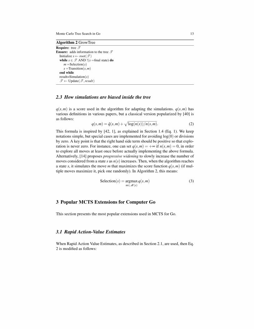
Algorithm 2 GrowTreeRequire: tree TEnsure: adds information to the tree T
Initialize s← root(T )while s ∈T AND !(s =final state) do
m =Selection(s)s =Transition(s,m)
end whileresult=Simulation(s)T ← Update(T ,result)
2.3 How simulations are biased inside the tree
q(s,m) is a score used in the algorithm for adapting the simulations. q(s,m) hasvarious definitions in various papers, but a classical version popularized by [40] isas follows:
q(s,m) = q(s,m)+√
log(n(s))/n(s,m). (2)
This formula is inspired by [42, 1], as explained in Section 1.4 (Eq. 1). We keepnotations simple, but special cases are implemented for avoiding log(0) or divisionsby zero. A key point is that the right hand side term should be positive so that explo-ration is never zero. For instance, one can set q(s,m) = +∞ if n(s,m) = 0, in orderto explore all moves at least once before actually implementing the above formula.Alternatively, [14] proposes progressive widening to slowly increase the number ofmoves considered from a state s as n(s) increases. Then, when the algorithm reachesa state s, it simulates the move m that maximizes the score function q(s,m) (if mul-tiple moves maximize it, pick one randomly). In Algorithm 2, this means:
Selection(s) = argmaxm∈M (s)
q(s,m) (3)
3 Popular MCTS Extensions for Computer Go
This section presents the most popular extensions used in MCTS for Go.
3.1 Rapid Action-Value Estimates
When Rapid Action Value Estimates, as described in Section 2.1, are used, then Eq.2 is modified as follows:

14 Adrien Couetoux and Martin Muller and Olivier Teytaud
q(s,m) = α(q(s,m)+√
log(n(s))/n(s,m))
+ (1−α)(qrave(s,m)+√
log(nrave(s))/nrave(s,m)) (4)
where q(s,m) and qrave(s,m) are defined in Section 2.1. This score linearly com-bines two move scores:
• The classical UCT score consisting of the average payoff q(s,m) plus an explo-ration term; this part is based on simulations in which move m has been playedimmediately in state s.
• The RAVE score of m in s is computed from all simulations in which m has beenplayed in s or later in the simulation. These simulations are termed RAVE sim-ulations. Importantly, RAVE simulations are the same as classical simulations;just, the set of simulations used for valuating a move m is (see Section 2.1)
– Simulations(m,s): Simulations in which m is played in s;– Rave−Simulations(m,s): Simulations in which m is played in s or later.
The union of the Simulations(m,s), for all m legal in s, is equal to the unionof the Rave− Simulations(m,s); but for a fixed m, Rave− Simulations(m,s) ismuch bigger than Simulations(m,s). For a typical state s, each simulation con-taining s appears in only one Simulation(m,s), and in many different Rave−Simulation(m,s).
The RAVE term is, a priori, less precise than the classical UCT term. However,RAVE produces statistics much more quickly. On average, almost half the moveson the board are played at least once by one player over the course of a wholesimulation, whereas there is only a single move per simulation from state s. RAVEvalues are therefore most useful in the early phase of a search, when there are onlyfew simulations for a given move. Therefore, the coefficient α must go to 1 whenthe number of simulations increases, and should be 0 when there are only RAVEsimulations in a node. A classical formula [31] is
α =√
n(s,m)/(n(s,m)+3k)
where k is chosen so that when n(s,m) = k, the RAVE value qrave(s,m) and theclassical value q(s,m) have nearly the same weight.
In most strong Go programs, RAVE is used and gives a clear improvement. How-ever, it can fail occasionally [47], in the case where a move must be played immedi-ately, but is often bad when played later in a simulation. Figure 5 shows an examplewhere the program FUEGO does not find the only winning move due to its badRAVE score.

Monte Carlo Tree Search in Go 15
Fig. 5 Example of misleading RAVE score in FUEGO: White B2 is the only winning movewhich avoids a seki. Its RAVE value is very low, since if the liberty at A5 gets filled first, ashappens in many simulations, then B2 becomes a very bad self-atari.
3.2 Learning and using local Go patterns
Go players learn many patterns - local shapes of stones - as well as informationsuch as which moves in a pattern are forced, usually good, or bad. All such rules areheuristic and cannot be used for hard pruning.
For example, playing a so-called empty triangle is usually bad shape, but in somecases it can be a good move. Figure 6 shows examples. Databases of patterns areused in all strong MCTS programs for both simulations and, to an even larger de-gree, as in-tree knowledge. While some programs play standard joseki sequencesinstantly, most patterns are used as a soft bias only. This allows a bad shape moveto still be simulated and chosen by the search.
Section 3.2.1 discusses the learning of patterns. Section 3.2.2 presents the use ofpatterns in the game tree (defining pattern values, and using pattern values for bias-ing the tree search). Section 3.2.3 is dedicated to patterns in the playouts (definingvalues, and using pattern values for biasing the Monte Carlo sampling, out of thetree).

16 Adrien Couetoux and Martin Muller and Olivier Teytaud
Fig. 6 Do not play empty triangles (usually): Playing K11 or L12 for Black builds an emptytriangle; it wastes one stone with little effect. Counter-example: On the other hand playing G6 forblack is a good move; it is the only solution for killing E6.
3.2.1 Patterns Learning
Learning patterns is not an easy task. [19, 14] learn the value of patterns in databases.Let us consider a database of games between strong players. The pattern is a familyof pairs (relative location, set of values); for example, an empty triangle pattern (Fig.6) is “(-1,0) is black, (0,1) is black, (-1,1) is empty, next move is (0,0)”. The mostpopular patterns shapes are approximately circular and rectangular/square. Specialcase patterns can be learned for corners and sides of the board. Standard corneropening sequences called joseki can also be represented as sets of patterns. Formatching, symmetries such as rotation, mirroring and swapping colors are takeninto account.
The confidence of a pattern is the probability (in the database) that a pattern isplayed, given that it can be played legally. The support of a pattern is the frequencyat which simultaneously (i) the pattern can legally be played and (ii) it is actu-ally played. There are fast algorithms for selecting patterns which have at least agiven support and a given confidence [7]; the speed strongly depends on the supportthreshold (the lower the threshold, the slower the algorithm).
Monte Carlo Tree Search in Go 17
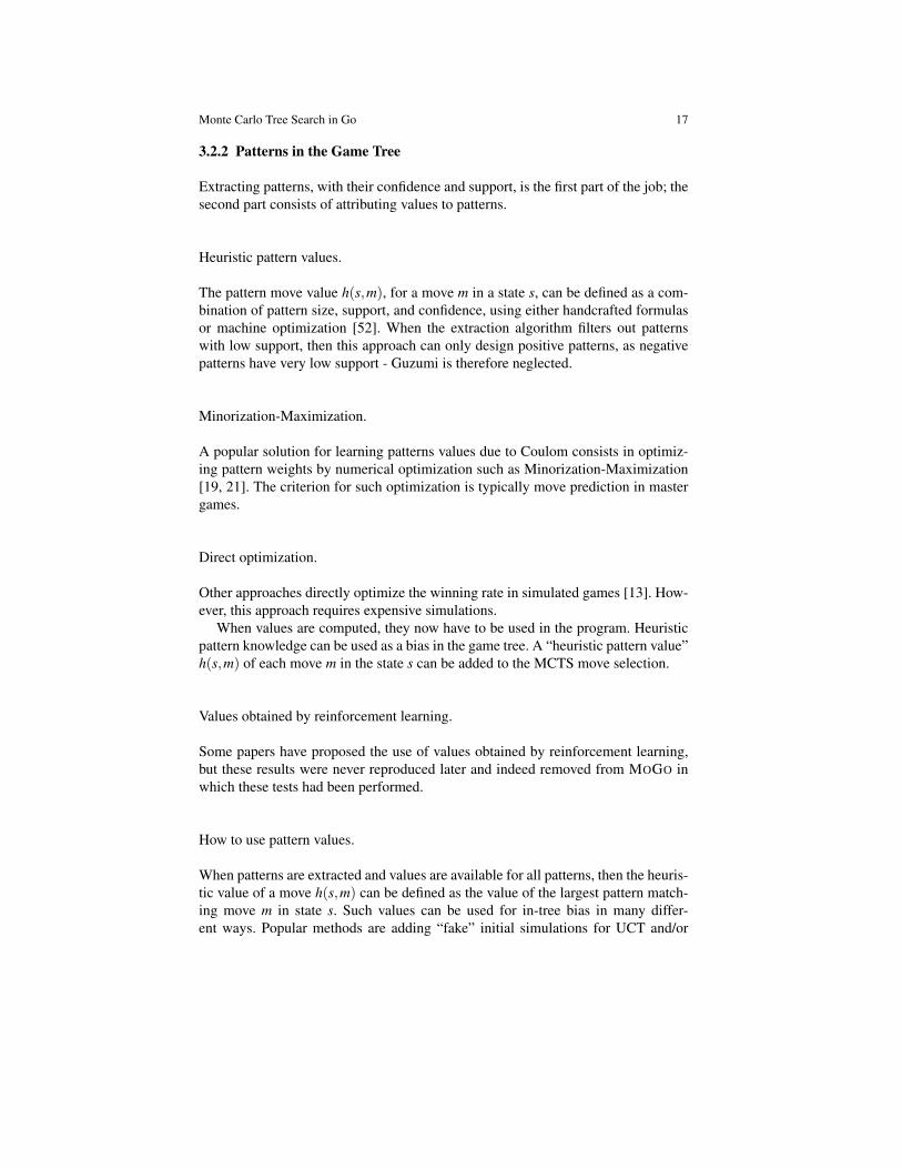
3.2.2 Patterns in the Game Tree
Extracting patterns, with their confidence and support, is the first part of the job; thesecond part consists of attributing values to patterns.
Heuristic pattern values.
The pattern move value h(s,m), for a move m in a state s, can be defined as a com-bination of pattern size, support, and confidence, using either handcrafted formulasor machine optimization [52]. When the extraction algorithm filters out patternswith low support, then this approach can only design positive patterns, as negativepatterns have very low support - Guzumi is therefore neglected.
Minorization-Maximization.
A popular solution for learning patterns values due to Coulom consists in optimiz-ing pattern weights by numerical optimization such as Minorization-Maximization[19, 21]. The criterion for such optimization is typically move prediction in mastergames.
Direct optimization.
Other approaches directly optimize the winning rate in simulated games [13]. How-ever, this approach requires expensive simulations.
When values are computed, they now have to be used in the program. Heuristicpattern knowledge can be used as a bias in the game tree. A “heuristic pattern value”h(s,m) of each move m in the state s can be added to the MCTS move selection.
Values obtained by reinforcement learning.
Some papers have proposed the use of values obtained by reinforcement learning,but these results were never reproduced later and indeed removed from MOGO inwhich these tests had been performed.
How to use pattern values.
When patterns are extracted and values are available for all patterns, then the heuris-tic value of a move h(s,m) can be defined as the value of the largest pattern match-ing move m in state s. Such values can be used for in-tree bias in many differ-ent ways. Popular methods are adding “fake” initial simulations for UCT and/or

18 Adrien Couetoux and Martin Muller and Olivier Teytaud
RAVE values with “virtual wins and losses”, or directly adding a term such asC×h(s,m)/ log(n(s,m)) to the move selection formula [52].
Pattern matching can be based on hashing and be reasonably fast [19]. Values arecomputed once for a node when it is created. Some implementations maintain twotypes of nodes; small nodes before computing the pattern value of each move, andlarge nodes for which values have been computed.
3.2.3 Patterns in the Playouts
Using patterns in playouts is important, but computationally much more challengingsince typical playouts aim for a speed in the order of one microsecond per move. Be-sides the still popular small handcrafted patterns such as the original 3×3 “MOGOpatterns” [66] (accompanied by expert rules such as “if you can capture, then cap-ture”, and, for advanced programs, more sophisticated Go expertise such as Nakadeand approach moves), we distinguish two learning methods:
• Offline learning: patterns are learnt before the actual game is played.• Online learning: patterns are learnt during the actual game.
Offline learning of pattern values for Monte Carlo Simulations
An early negative result by Gelly and Silver showed that increasing the strengthof a Monte Carlo simulation policy does not necessarily improve the strength ofthe MCTS player built on top of it [29, 66]. It is more important that a playoutis “unbiased” or “balanced”, i.e. that black moves and white moves preserve theequilibrium of the game [61, 35]. Therefore a possible solution consists in definingthe balancing problem for N parameters θ = (θ1, . . . ,θN) as follows:
• Vθ (s): the frequency of wins over M simulations for black when playouts start insituation s and use parameters θ .
• Vtarget(s): a target value, obtained either:
– by human expertise;– or by self-play of a MCTS program on situation s.
The case of learning from self-play is particularly interesting because it is unsuper-vised.
Given Vtarget(s) and a parametric policy defining simulations as a function of aparameter θ , SB provides a parameter θ is obtained by minimization of
θ = argminθ
∑s∈{s1,...,sN}
(Vθ (s)−Vtarget(s))2 . (5)
Let us define the random variable simulation, which is defined for some initial states and a parameter θ . The derivative, with respect to θ , of the sum of squares term inEq. 5 is the product of
Monte Carlo Tree Search in Go 19
2Es (Vθ (s)−Vtarget(s))
(which is easy to compute by simulations, given θ and Vtarget and
Esimulationreward(simulation)∇θ logP(simulation|s,θ),
which needs the gradient of the log-likelihood logP(simulation|s,θ), which is thesum of the log-likelihood of each move in the simulation.
Success has been reported for simulation balancing on small boards and for theGo program ERICA [34]. However, some negative results were also reported onthe computer-go mailing list; sometimes, minimizing Eq. 5 actually decreased theplaying strength of the MCTS built on top of the playout.
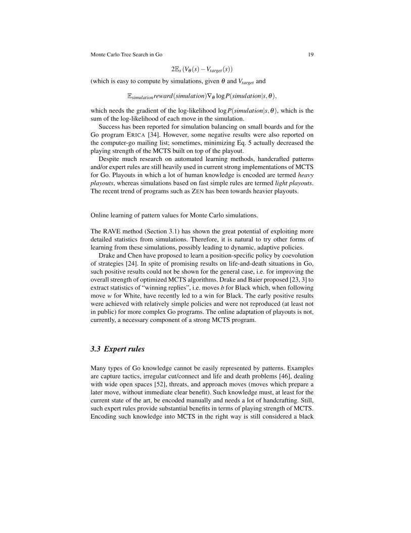
Despite much research on automated learning methods, handcrafted patternsand/or expert rules are still heavily used in current strong implementations of MCTSfor Go. Playouts in which a lot of human knowledge is encoded are termed heavyplayouts, whereas simulations based on fast simple rules are termed light playouts.The recent trend of programs such as ZEN has been towards heavier playouts.
Online learning of pattern values for Monte Carlo simulations.
The RAVE method (Section 3.1) has shown the great potential of exploiting moredetailed statistics from simulations. Therefore, it is natural to try other forms oflearning from these simulations, possibly leading to dynamic, adaptive policies.
Drake and Chen have proposed to learn a position-specific policy by coevolutionof strategies [24]. In spite of promising results on life-and-death situations in Go,such positive results could not be shown for the general case, i.e. for improving theoverall strength of optimized MCTS algorithms. Drake and Baier proposed [23, 3] toextract statistics of “winning replies”, i.e. moves b for Black which, when followingmove w for White, have recently led to a win for Black. The early positive resultswere achieved with relatively simple policies and were not reproduced (at least notin public) for more complex Go programs. The online adaptation of playouts is not,currently, a necessary component of a strong MCTS program.
3.3 Expert rules
Many types of Go knowledge cannot be easily represented by patterns. Examplesare capture tactics, irregular cut/connect and life and death problems [46], dealingwith wide open spaces [52], threats, and approach moves (moves which prepare alater move, without immediate clear benefit). Such knowledge must, at least for thecurrent state of the art, be encoded manually and needs a lot of handcrafting. Still,such expert rules provide substantial benefits in terms of playing strength of MCTS.Encoding such knowledge into MCTS in the right way is still considered a black

20 Adrien Couetoux and Martin Muller and Olivier Teytaud
art. Parameter tuning methods can help, but surprisingly little has been published onthis topic.
3.4 Global and local opening books - Fuseki and Joseki
Full board opening books specify the next move given an exactly matching board.They are limited for the full 19× 19 board in Go due to the large branching factorand diversity of possible moves. However, on board sizes of 9×9 and smaller, booksare very powerful. On 7×7, the MOGO program has shown better than professionalperformance thanks to its huge opening book built by self-play by a “meta” MCTSalgorithm, using a MCTS algorithm as default policy [17]. Importantly, the processstill involves some human intervention and trial-and-error.
For big boards (13× 13 and 19× 19), books can also be used for joseki, localopening sequences. The corners and sides are very important in Go, since it is mucheasier to build territories and eyes there. “Joseki” refers to standard sequences ina single corner, which are usually but not always played out in the opening phase.In contrast, the term fuseki refers to full board openings, and in part deals withthe interaction between different corners and sides. Many current MCTS programsinclude large-scale patterns, covering josekis and even full board positions. They areusually used for soft pruning, as explained in Section 3.2.2, rather than hardcodedmoves.
3.5 Parallelizing MCTS for Go
Despite some inherent limitations as discussed above, MCTS generally scales wellwith increasing time and memory. More simulations and larger trees result instronger play, with no apparent upper limit in complex games such as Go. To achievegood performance on current hardware such as multicore machines, computer clus-ters and supercomputers, it is necessary to parallelize MCTS.
Unfortunately, this is a highly nontrivial problem. It is easy to run simulationsin parallel. However, the returns from running more simulations on the same nodediminish very quickly [72]. The true power of MCTS comes from using the resultsof previous simulations to grow the tree and choose where future simulations startfrom, so it is inherently a sequential algorithm. This imposes both theoretical limitsand practical challenges to parallelization.
The two main types of parallel MCTS are differentiated by the memory model.Multi-core machines such as workstations provide a single shared memory, whileclusters with distributed memory architecture require an approach using message-passing. On large-scale modern machines with fast networks and a multi-level mem-ory hierarchy this formerly clear distinction begins to blur. We discuss the main al-

Monte Carlo Tree Search in Go 21
gorithms for different architectures, then present theoretical scalability issues whichlimit the efficiency of parallelization.
Besides the works discussed in more detail below, other important publicationson parallel MCTS in Go include [11, 15, 37, 32].
3.5.1 Shared Memory Parallelization on a Multi-core Machine
Parallelizing MCTS on a multi-core machine is usually performed by running theloop of MCTS (Section 2.2) simultaneously on each core, with each core updatingthe same game tree in memory. The two main limitations are memory contentionand diversity of simulations. Memory contention occurs whenever different threadsaccess the same memory location representing the same node. Increasing the num-ber of threads also puts strain on the memory bus systems. Locking the tree for eachupdate is not a realistic option - lock-free algorithms are required [20, 26]. The otherrisk is that without global control, all cores will run very similar simulations. Thetechnique of virtual loss [15] temporarily adds a loss to the tree before the simula-tion is run. This encourages other threads to explore different parts of the tree. Ifthe simulation turns out to be a win, the virtual loss is changed accordingly. Someauthors have also experimented with virtual wins.
3.5.2 Parallelization with message passing
On message-passing machines such as off-the-shelf clusters, it is too slow to sharememory directly. A classical solution [11, 5] used in MOGO works as follows:
• A separate MCTS runs on each machine.• With low frequency, such as three times per second, all nodes broadcast statistics
such as number of simulations, number of wins, number of RAVE simulations,and number of RAVE wins for all “heavy” nodes which have been included in atleast some percentage of the total number of simulations. Such broadcast can beperformed in time logarithmic in the number of machines if the network structuresupports it.
• Each node augments its statistics using these messages and keeps running.
3.5.3 Parallelization with Distributed Tree and Depth-First UCT
One severe disadvantage of the solution above is the large amount of duplication.Many trees are built concurrently, each starting from the root, and due to the par-tial synchronisation there is a large amount of overlap between them. It is thereforetempting to develop methods where a single tree is distributed over all nodes ina parallel system. UCT-Treesplit is one such approach, used in the program GO-MORRA [32]. Another major bottleneck to parallelization is that in the classical for-mulation of MCTS, each simulation result is propagated all the way to the root node.
22 Adrien Couetoux and Martin Muller and Olivier Teytaud
This causes heavy memory contention near the root, which limits speedup. Depth-first UCT [73] is a reformulation of UCT which drastically reduces the number ofsuch updates at only a small loss in precision of in-tree move selection. It is usedin conjunction with a distributed transposition table in MPFUEGO, the massivelyparallel version of FUEGO.
3.5.4 Limits to Scalability
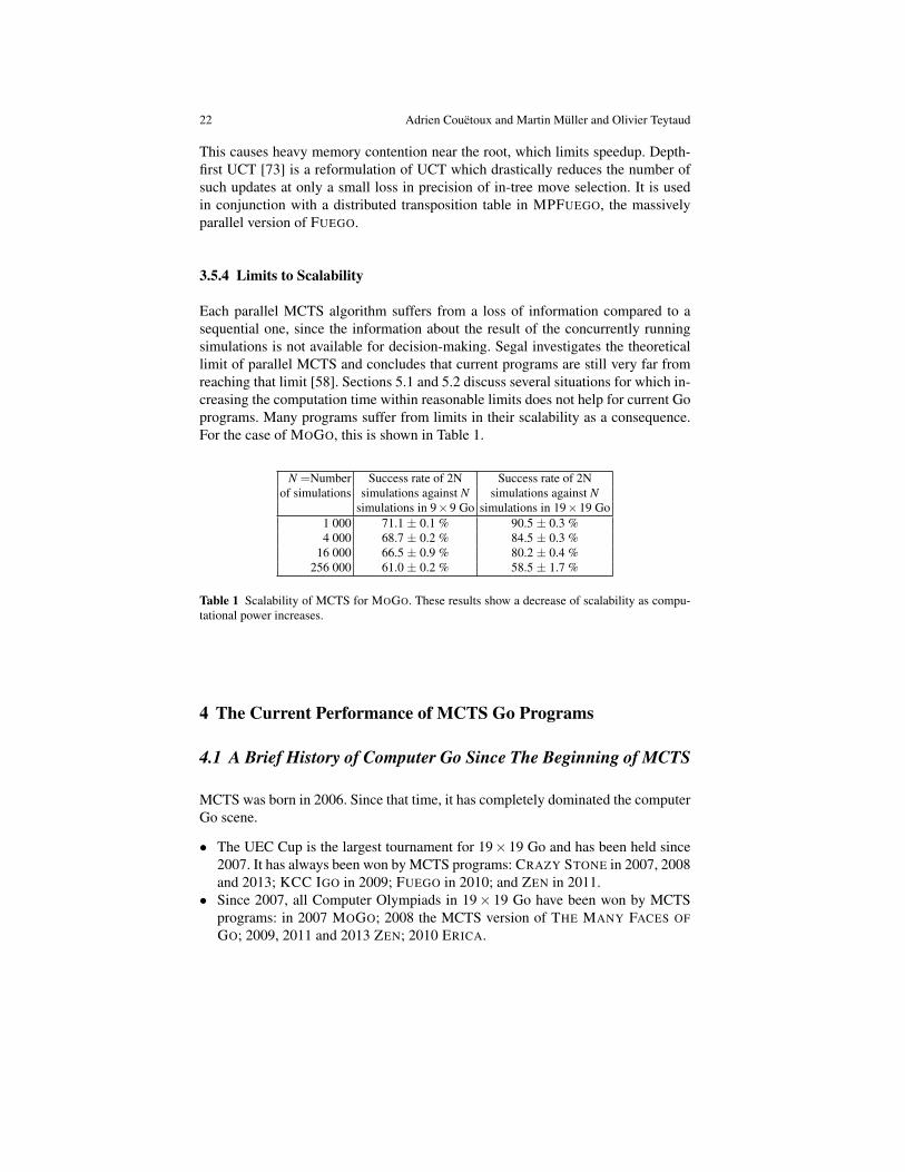
Each parallel MCTS algorithm suffers from a loss of information compared to asequential one, since the information about the result of the concurrently runningsimulations is not available for decision-making. Segal investigates the theoreticallimit of parallel MCTS and concludes that current programs are still very far fromreaching that limit [58]. Sections 5.1 and 5.2 discuss several situations for which in-creasing the computation time within reasonable limits does not help for current Goprograms. Many programs suffer from limits in their scalability as a consequence.For the case of MOGO, this is shown in Table 1.
N =Number Success rate of 2N Success rate of 2Nof simulations simulations against N simulations against N
simulations in 9×9 Go simulations in 19×19 Go1 000 71.1 ± 0.1 % 90.5 ± 0.3 %4 000 68.7 ± 0.2 % 84.5 ± 0.3 %
16 000 66.5 ± 0.9 % 80.2 ± 0.4 %256 000 61.0 ± 0.2 % 58.5 ± 1.7 %
Table 1 Scalability of MCTS for MOGO. These results show a decrease of scalability as compu-tational power increases.
4 The Current Performance of MCTS Go Programs
4.1 A Brief History of Computer Go Since The Beginning of MCTS
MCTS was born in 2006. Since that time, it has completely dominated the computerGo scene.
• The UEC Cup is the largest tournament for 19×19 Go and has been held since2007. It has always been won by MCTS programs: CRAZY STONE in 2007, 2008and 2013; KCC IGO in 2009; FUEGO in 2010; and ZEN in 2011.
• Since 2007, all Computer Olympiads in 19× 19 Go have been won by MCTSprograms: in 2007 MOGO; 2008 the MCTS version of THE MANY FACES OFGO; 2009, 2011 and 2013 ZEN; 2010 ERICA.
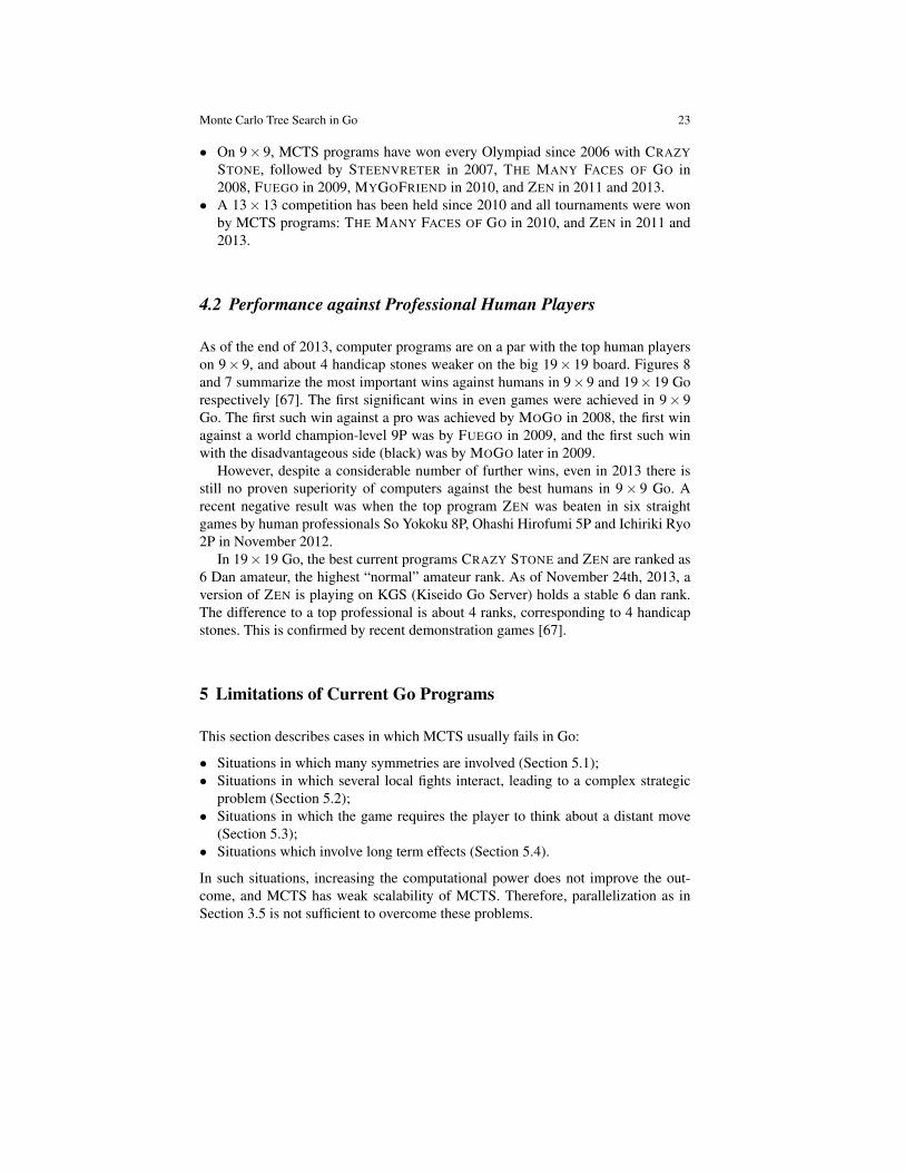
Monte Carlo Tree Search in Go 23
• On 9× 9, MCTS programs have won every Olympiad since 2006 with CRAZYSTONE, followed by STEENVRETER in 2007, THE MANY FACES OF GO in2008, FUEGO in 2009, MYGOFRIEND in 2010, and ZEN in 2011 and 2013.
• A 13× 13 competition has been held since 2010 and all tournaments were wonby MCTS programs: THE MANY FACES OF GO in 2010, and ZEN in 2011 and2013.
4.2 Performance against Professional Human Players
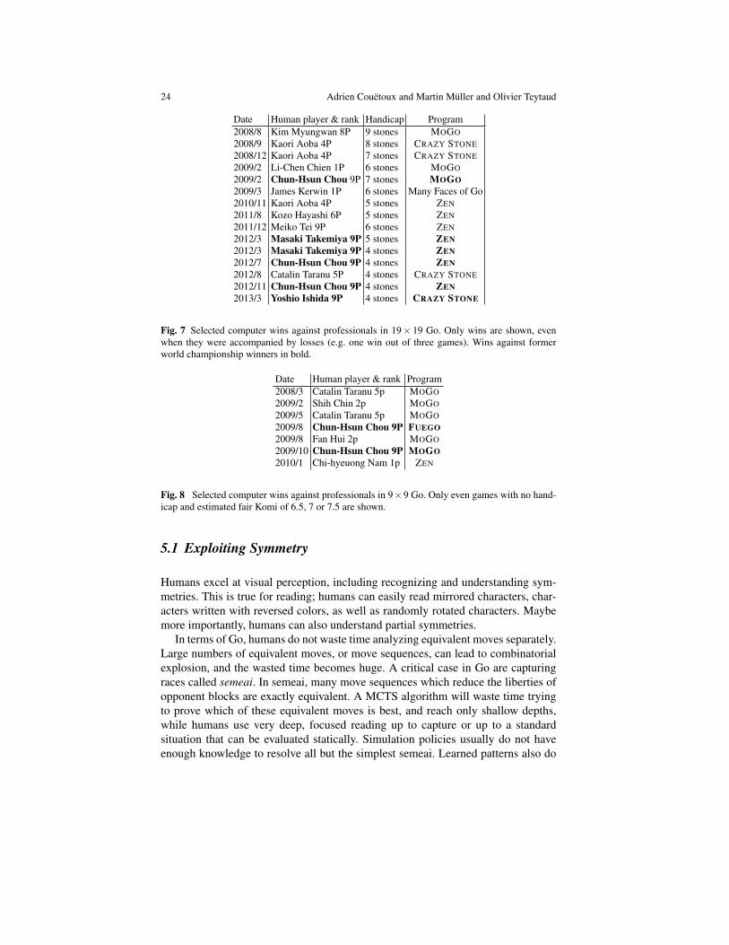
As of the end of 2013, computer programs are on a par with the top human playerson 9× 9, and about 4 handicap stones weaker on the big 19× 19 board. Figures 8and 7 summarize the most important wins against humans in 9×9 and 19×19 Gorespectively [67]. The first significant wins in even games were achieved in 9× 9Go. The first such win against a pro was achieved by MOGO in 2008, the first winagainst a world champion-level 9P was by FUEGO in 2009, and the first such winwith the disadvantageous side (black) was by MOGO later in 2009.
However, despite a considerable number of further wins, even in 2013 there isstill no proven superiority of computers against the best humans in 9× 9 Go. Arecent negative result was when the top program ZEN was beaten in six straightgames by human professionals So Yokoku 8P, Ohashi Hirofumi 5P and Ichiriki Ryo2P in November 2012.
In 19×19 Go, the best current programs CRAZY STONE and ZEN are ranked as6 Dan amateur, the highest “normal” amateur rank. As of November 24th, 2013, aversion of ZEN is playing on KGS (Kiseido Go Server) holds a stable 6 dan rank.The difference to a top professional is about 4 ranks, corresponding to 4 handicapstones. This is confirmed by recent demonstration games [67].
5 Limitations of Current Go Programs
This section describes cases in which MCTS usually fails in Go:
• Situations in which many symmetries are involved (Section 5.1);• Situations in which several local fights interact, leading to a complex strategic
problem (Section 5.2);• Situations in which the game requires the player to think about a distant move
(Section 5.3);• Situations which involve long term effects (Section 5.4).
In such situations, increasing the computational power does not improve the out-come, and MCTS has weak scalability of MCTS. Therefore, parallelization as inSection 3.5 is not sufficient to overcome these problems.
24 Adrien Couetoux and Martin Muller and Olivier Teytaud
Date Human player & rank Handicap Program2008/8 Kim Myungwan 8P 9 stones MOGO2008/9 Kaori Aoba 4P 8 stones CRAZY STONE2008/12 Kaori Aoba 4P 7 stones CRAZY STONE2009/2 Li-Chen Chien 1P 6 stones MOGO2009/2 Chun-Hsun Chou 9P 7 stones MOGO2009/3 James Kerwin 1P 6 stones Many Faces of Go2010/11 Kaori Aoba 4P 5 stones ZEN2011/8 Kozo Hayashi 6P 5 stones ZEN2011/12 Meiko Tei 9P 6 stones ZEN2012/3 Masaki Takemiya 9P 5 stones ZEN2012/3 Masaki Takemiya 9P 4 stones ZEN2012/7 Chun-Hsun Chou 9P 4 stones ZEN2012/8 Catalin Taranu 5P 4 stones CRAZY STONE2012/11 Chun-Hsun Chou 9P 4 stones ZEN2013/3 Yoshio Ishida 9P 4 stones CRAZY STONE
Fig. 7 Selected computer wins against professionals in 19× 19 Go. Only wins are shown, evenwhen they were accompanied by losses (e.g. one win out of three games). Wins against formerworld championship winners in bold.
Date Human player & rank Program2008/3 Catalin Taranu 5p MOGO2009/2 Shih Chin 2p MOGO2009/5 Catalin Taranu 5p MOGO2009/8 Chun-Hsun Chou 9P FUEGO2009/8 Fan Hui 2p MOGO2009/10 Chun-Hsun Chou 9P MOGO2010/1 Chi-hyeuong Nam 1p ZEN
Fig. 8 Selected computer wins against professionals in 9×9 Go. Only even games with no hand-icap and estimated fair Komi of 6.5, 7 or 7.5 are shown.
5.1 Exploiting Symmetry
Humans excel at visual perception, including recognizing and understanding sym-metries. This is true for reading; humans can easily read mirrored characters, char-acters written with reversed colors, as well as randomly rotated characters. Maybemore importantly, humans can also understand partial symmetries.
In terms of Go, humans do not waste time analyzing equivalent moves separately.Large numbers of equivalent moves, or move sequences, can lead to combinatorialexplosion, and the wasted time becomes huge. A critical case in Go are capturingraces called semeai. In semeai, many move sequences which reduce the liberties ofopponent blocks are exactly equivalent. A MCTS algorithm will waste time tryingto prove which of these equivalent moves is best, and reach only shallow depths,while humans use very deep, focused reading up to capture or up to a standardsituation that can be evaluated statically. Simulation policies usually do not haveenough knowledge to resolve all but the simplest semeai. Learned patterns also do

Monte Carlo Tree Search in Go 25
Fig. 9 White to play. In the 8 vs 8 liberty semeai at the bottom, White must immediately attackthe black group J4 by taking one of its liberties. This also saves M4.
not help since the liberty-filling moves are usually not good shape and have no othermeaning than to kill.
As a consequence, no current MCTS program can distinguish reliably betweensituations like Fig. 9, which is a semeai which must be played immediately, and Fig.10, a semeai which has been decided.
5.2 Local Search for Divide and Conquer
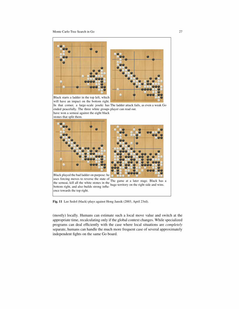
MCTS has provided great improvements in the general fighting ability of Go pro-grams. However, they have trouble handling multiple simultaneous fights. Huangand Muller study two such cases, termed “two safe groups” and seki (coexistence)[36]. They develop a test suite of such problems and test it against most of the cur-rent top programs. These problems contain simple local fights, but are too deep to bejointly resolved by global search. Only very few programs have enough knowledgein their simulation policy to do well. A famous example of a professional gamewhere two local fights interact in a complex way is shown in Fig. 11.
Divide and conquer approaches have been successful for endgame puzzles [44]and for small isolated life-and-death problems [38], but not yet in the context of afull board MCTS program. Sheppard [59] proposed the use of MCTS with macro-

26 Adrien Couetoux and Martin Muller and Olivier Teytaud
Fig. 10 Black to play is ahead by 8 vs 6 liberties and should not play in the semeai - it would be awasted move.
actions. This looks reasonable, but as far as we know has not yet been successfullyimplemented.
5.3 The Art of Tenuki
One of the simplest expert rules used in MCTS algorithms is locality: very often, thebest move is close to the previous one. Deciding when to answer locally, and whento “tenuki”, i.e. switch to elsewhere on the board, is considered as a key competencefor playing Go. In terms of combinatorial game theory, it amounts to evaluating andcomparing the temperature - urgency of playing in - different parts of the board.Patterns and human expertise are good for helping MCTS in soft pruning, hencepartially counterbalance the bonus for local play.
An illustrative proverb says “If it’s worth only 15 points, play tenuki”. MCTSworks by simulations and wins and losses; the concept of points is not included inMCTS.
One computational inefficiency of the full-board, global search used in MCTSis that it needs to spend computational effort on a candidate tenuki move each timewhile playing out a local sequence. It cannot re-use computations about other partsof the board performed during earlier moves, since they are all embedded in anever-changing global context. In many cases, the value of a move can be computed
Monte Carlo Tree Search in Go 27
Black starts a ladder in the top left, whichwill have an impact on the bottom right.In that corner, a large-scale joseki hasended peacefully. The three white groupshave won a semeai against the eight blackstones that split them.
The ladder attack fails, as even a weak Goplayer can read out.
Black played the bad ladder on purpose: heuses forcing moves to reverse the state ofthe semeai, kill all the white stones in thebottom right, and also builds strong influ-ence towards the top right.
The game at a later stage. Black has ahuge territory on the right side and wins.
Fig. 11 Lee Sedol (black) plays against Hong Jansik (2003, April 23rd).
(mostly) locally. Humans can estimate such a local move value and switch at theappropriate time, recalculating only if the global context changes. While specializedprograms can deal efficiently with the case where local situations are completelyseparate, humans can handle the much more frequent case of several approximatelyindependent fights on the same Go board.

28 Adrien Couetoux and Martin Muller and Olivier Teytaud
5.4 Long-Term Effects
Some situations require subtle moves which have a long-term impact. Similarly,moves can be bad because of a long-term negative effect. Long-term effects aredifficult for MCTS since they can not be handled in the tree - they are only resolvedin the (noisy, low quality) simulation phase. Avoiding moves with such bad long-term effects is a major open problem for MCTS in Go, and is discussed in somedetail in this section.
MCTS simulations consist of two parts:
• an in-tree part containing (reasonably) good moves;• Monte Carlo simulations or playouts, which are randomized and contain many
blunders.
As a consequence, later parts of the game are very poorly simulated. This is actuallymuch improved when heavy playouts are used. Yet, the quality is much better forin-tree moves. This implies that a move which has bad long term consequencesis not reliably evaluated as bad by the simulations. Besides the cases of two safegroups and seki mentioned in Section 5.2, Ko fights are a classic example. In Figure12, White can save the group at the top late in the game because White has a Kothreat at the bottom. However, most MCTS programs would have played the forcingexchange F2 for F1 much earlier in the game, and as a consequence they would beout of Ko threats at this stage. Therefore, it is important to not to waste threats, andkeep them for Ko fights that might materialize later. Most MCTS programs are notable to do that, for (at least) two reasons. One problem is that locally, F2 is a goodmove, gaining one point in sente. However, it is more important to keep it in reserveas a threat until late in the endgame. Another problem is specific to MCTS withits evaluation of a node as the weighted average of its children. A threat which hasonly one good reply will have a too-high value, since it inherits some of the highevaluations for all the other branches where the opponent ignored the threat. In theexample, if White plays F2 and Black answers anywhere else but F1, then all thesepositions will be big wins for White.
6 Conclusions
Currently all strong Go programs are based on MCTS. In the early days of MCTS forGo, it was possible to design such a program without any expertise in Go, using justlight playouts. However, introducing human expertise is now critical for reachinga competitive playing level; all strong programs use such knowledge in the play-outs and in the tree. This knowledge can be partially learnt offline, automatically,on databases of games; and online, thanks to RAVE values. Also results can be im-proved by the parallelization on multi-core machines or clusters. Unfortunately, aswith classical programs, the key bottleneck remains the encoding of human exper-

Monte Carlo Tree Search in Go 29
Fig. 12 The importance of keeping Ko threats. Left: Black captures the Ko with C8, leadingto the middle position. Middle: White can not immediately recapture at C7 due to the Ko rule, butWhite can play a Ko threat at F2, leading to the position on the right. Right: if Black ignores thethreat, White will play F1 next and kill the bottom side. If Black plays F1, White can now recaptureat C7. Black has no threats, so White can also connect at C8 and live. Thanks to the threat at F2,White won the Ko fight and lived.
tise, despite progress in automated methods such as large-scale learning of patternweights.
Future Work and Open Problems
There are many clearly defined situations which are poorly handled by MCTS Goprograms, such as divide and conquer problems, semeai, and long term effects suchas Ko threats. While a lot of research has been devoted to these problems, includingonline or offline learning, many challenges still remain unsolved.
Acknowledgments
We are grateful to Shi-Jim Yen for fruitful discussions.
References
1. P. Auer, N. Cesa-Bianchi, and P. Fischer. Finite time analysis of the multiarmed bandit prob-lem. Machine Learning, 47(2/3):235–256, 2002.
2. P. Auer, N. Cesa-Bianchi, Y. Freund, and R. E. Schapire. Gambling in a rigged casino: the ad-versarial multi-armed bandit problem. In Proceedings of the 36th Annual Symposium on Foun-dations of Computer Science, pages 322–331. IEEE Computer Society Press, Los Alamitos,CA, 1995.
3. H. Baier and P. Drake. The power of forgetting: Improving the last-good-reply policy in MonteCarlo Go. IEEE Transactions on Computational Intelligence and AI in Games, 2(4):303–309,2010.
30 Adrien Couetoux and Martin Muller and Olivier Teytaud
4. D. Benson. Life in the game of Go. Information Sciences, 10:17–29, 1976. Reprinted inComputer Games, Levy, D.N.L. (Editor), Vol. II, pp. 203-213, Springer Verlag, New York1988.
5. A. Bourki, G. Chaslot, M. Coulm, V. Danjean, H. Doghmen, J.-B. Hoock, T. Herault, A. Rim-mel, F. Teytaud, O. Teytaud, P. Vayssiere, and Z. Yu. Scalability and parallelization of monte-carlo tree search. In Proceedings of Advances in Computer Games 13, 2010.
6. B. Bouzy and T. Cazenave. Computer Go: An AI-oriented survey. Artificial Intelligence,132(1):39–103, 2001.
7. B. Bouzy and G. Chaslot. Bayesian generation and integration of k-nearest-neighbor patternsfor 19x19 go. In G. Kendall and Simon Lucas, editors, IEEE 2005 Symposium on Computa-tional Intelligence in Games, Colchester, UK, pages 176–181, 2005.
8. R. Bozulich. The Go Players Almanac 2001. Kiseido, Tokyo, 2001.9. C. Browne, E. Powley, D. Whitehouse, S. Lucas, P. Cowling, P. Rohlfshagen, S. Tavener,
D. Perez, S. Samothrakis, and S. Colton. A survey of Monte Carlo tree search methods. IEEETrans. Comput. Intellig. and AI in Games, 4(1):1–43, 2012.
10. B. Bruegmann. Monte-carlo Go, 1993. Unpublished draft, http://www.althofer.de/Bruegmann-MonteCarloGo.pdf.
11. T. Cazenave and N. Jouandeau. On the parallelization of UCT. In Proceedings of CGW07,pages 93–101, 2007.
12. G. Chaslot, S. Bakkes, I. Szita, and P. Spronck. Monte Carlo Tree Search: A New Frameworkfor Game AI. In C. Darken and M. Mateas, editors, AIIDE. The AAAI Press, 2008.
13. G. Chaslot, M. Winands, I.Szita, and H. van den Herik. Parameter tuning by cross entropymethod. In European Workshop on Reinforcement Learning, 2008.
14. G. Chaslot, M. Winands, J. Uiterwijk, H. van den Herik, and B. Bouzy. Progressive Strategiesfor Monte-Carlo Tree Search. In P. Wang et al., editors, Proceedings of the 10th Joint Confer-ence on Information Sciences (JCIS 2007), pages 655–661. World Scientific Publishing Co.Pte. Ltd., 2007.
15. G. M. J.-B. Chaslot, M. H. M. Winands, and H. J. van den Herik. Parallel Monte-Carlo TreeSearch. In Proc. Comput. and Games, LNCS 5131, pages 60–71, Beijing, China, 2008.
16. B. E. Childs, J. H. Brodeur, and L. Kocsis. Transpositions and move groups in Monte CarloTree Search. In P. Hingston and L. Barone, editors, IEEE Symposium on ComputationalIntelligence and Games, pages 389–395. IEEE, 2008.
17. C.-W. Chou, P.-C. Chou, H. Doghmen, C.-S. Lee, T.-C. Su, F. Teytaud, and O. Teytaud. To-wards a solution of 7x7 Go with Meta-MCTS. In Proceedings of Advances in ComputerGames 2011, pages November 20–23, 2011, Tilburg University, The Netherlands, 2011.
18. R. Coulom. Efficient Selectivity and Backup Operators in Monte-Carlo Tree Search. In P.Ciancarini and H. J. van den Herik, editors, Proceedings of the 5th International Conferenceon Computers and Games, Turin, Italy, 2006.
19. R. Coulom. Computing elo ratings of move patterns in the game of go. In Computer GamesWorkshop, Amsterdam, The Netherlands, 2007.
20. R. Coulom. Lockless hash table and other parallel search ideas, 2008. http://www.mail-archive.com/[email protected]/msg07611.html.
21. R. Coulom. Clop: Confident local optimization for noisy black-box parameter tuning. InAdvances in Computer Games, pages 146–157. Springer Berlin Heidelberg, 2012.
22. M. Crasmaru and J. Tromp. Ladders are PSPACE-complete. In Computers and Games, pages241–249, 2000.
23. P. Drake. The last-good-reply policy for monte-carlo go. ICGA Journal, 32(4):221–227, 2009.24. P. Drake and Y.-P. Chen. Coevolving partial strategies for the game of go. In International
Conference on Genetic and Evolutionary Methods. CSREA Press, 2008.25. M. Enzenberger. Evaluation in go by a neural network using soft segmentation. 10th Advances
in Computer Games Conference, Graz, 2003.26. M. Enzenberger and M. Muller. A lock-free multithreaded Monte-Carlo tree search algorithm.
In J. van den Herik and P. Spronck, editors, Advances in Computer Games, volume 6048 ofLecture Notes in Computer Science, pages 14–20, Pamplona, Spain, 2010. Springer Verlag.
Monte Carlo Tree Search in Go 31
27. S. Flory and O. Teytaud. Upper confidence trees with short term partial information. InProcedings of EvoGames 2011, pages 153–162. Springer, 2011.
28. Free Software Foundation. GNU Go, 1989-2013. Date retrieved: Nov 18, 2013. http://www.gnu.org/software/gnugo/.
29. S. Gelly. Une contribution a l’apprendissage par renforcement ; application au ComputerGO. PhD thesis, Universite Paris-Sud - Paris XI, September 2007. Paris Universities Awardand 2nd Prize at Gilles Kahn - Academie des Sciences Awards.
30. S. Gelly and D. Silver. Combining online and offline knowledge in UCT. In ICML ’07:Proceedings of the 24th international conference on Machine learning, pages 273–280, NewYork, NY, USA, 2007. ACM Press.
31. S. Gelly and D. Silver. Monte-carlo tree search and rapid action value estimation in computergo. Artif. Intell., 175(11):1856–1875, July 2011.
32. T. Graf, U. Lorenz, M. Platzner, and L. Schaefers. Parallel Monte-Carlo Tree Search for HPCSystems. In Proc. 17th Int. Euro. Conf. Parallel Distrib. Comput., LNCS 6853, pages 365–376,Bordeaux, France, 2011.
33. M. D. Grigoriadis and L. G. Khachiyan. A sublinear-time randomized approximation algo-rithm for matrix games. Operations Research Letters, 18(2):53–58, Sep 1995.
34. S. Huang. New Heuristics for Monte Carlo Tree Search Applied to the Game of Go. PhDthesis, National Taiwan Normal University, 2011.
35. S.-C. Huang, R. Coulom, and S.-S. Lin. Monte-carlo simulation balancing in practice. In H. J.van den Herik, H. Iida, and A. Plaat, editors, Computers and Games, volume 6515 of LectureNotes in Computer Science, pages 81–92. Springer, 2010.
36. S.-C. Huang and M. Muller. Investigating the limits of Monte Carlo tree search methods incomputer Go, 2013. Accepted for Computers and Games 2013. 12 pp.
37. H. Kato and I. Takeuchi. Parallel Monte-Carlo Tree Search with Simulation Servers. In Proc.Int. Conf. Tech. Applicat. Artif. Intell., pages 491–498, Hsinchu City, Taiwan, 2010.
38. A. Kishimoto and M. Muller. Dynamic decomposition search: A divide and conquer approachand its application to the one-eye problem in go. In IEEE Symposium on ComputationalIntelligence and Games (CIG’05), pages 164–170, 2005.
39. A. Kishimoto and M. Muller. Search versus knowledge for solving life and death problems inGo. In Twentieth National Conference on Artificial Intelligence (AAAI-05), pages 1374–1379,2005.
40. L. Kocsis and C. Szepesvari. Bandit based Monte-Carlo planning. In 15th European Confer-ence on Machine Learning (ECML), pages 282–293, 2006.
41. L. Kocsis and C. Szepesvari. Discounted-UCB. In 2nd Pascal-Challenge Workshop, 2006.42. T. Lai and H. Robbins. Asymptotically efficient adaptive allocation rules. Advances in Applied
Mathematics, 6:4–22, 1985.43. M. Muller. Playing it safe: Recognizing secure territories in computer Go by using static
rules and search. In H. Matsubara, editor, Game Programming Workshop in Japan ’97, pages80–86, Computer Shogi Association, Tokyo, Japan, 1997.
44. M. Muller. Decomposition search: A combinatorial games approach to game tree search, withapplications to solving Go endgames. In Sixteenth International Joint Conference on ArtificialIntelligence (IJCAI-99), pages 578–583, Stockholm, Sweden, 1999.
45. M. Muller. Review: Computer Go 1984 - 2000. In T. Marsland and I. Frank, editors, Com-puters and Games 2000, number 2063 in Lecture Notes in Computer Science, pages 426–435.Springer Verlag, 2001.
46. M. Muller. Computer Go. Artificial Intelligence, 134(1–2):145–179, 2002.47. M. Muller. Rave problems, 2009. http://www.mail-archive.com/
[email protected]/msg12189.html.48. X. Niu, A. Kishimoto, and M. Muller. Recognizing seki in computer Go. In J. van den Herik,
S.-C. Hsu, T.-s. Hsu, and H. Donkers, editors, Advances in Computer Games, volume 4250 ofLecture Notes in Computer Science, pages 88 – 103. Springer, 2006.
49. X. Niu and M. Muller. An open boundary safety-of-territory solver for the game of Go. InJ. van den Herik, P. Ciancarini, and H. Donkers, editors, Computers and Games, volume 4630of Lecture Notes in Computer Science, pages 37 – 49, Torino, Italy, 2007. Springer.
32 Adrien Couetoux and Martin Muller and Olivier Teytaud
50. X. Niu and M. Muller. An improved safety solver in Go using partial regions. In J. van denHerik, X. Xu, Z. Ma, and M. Winands, editors, Computers and Games, volume 5131 of LectureNotes in Computer Science, pages 102–112, Beijing, China, 2008. Springer.
51. W. Reitman and B. Wilcox. The structure and performance of the Interim.2 Go program. InIJCAI-79, pages 711–719, 1979.
52. A. Rimmel, O. Teytaud, C.-S. Lee, S.-J. Yen, M.-H. Wang, and S.-R. Tsai. Current Frontiersin Computer Go. IEEE Transactions on Computational Intelligence and Artificial Intelligencein Games, page in press, 2010.
53. B. Robertie. Backgammon. Inside Backgammon, 2(1):4, 1980.54. J. M. Robson. The complexity of go. In IFIP Congress, pages 413–417, 1983.55. A. Saffidine, T. Cazenave, and J. Mehat. UCD : Upper confidence bound for rooted directed
acyclic graphs. Knowl.-Based Syst., 34:26–33, 2012.56. J. Schaeffer. The history heuristic and alphavbeta search enhancements in practice. IEEE
Transactions on Pattern Analysis and Machine Intelligence PAMI-11, pages 1203–1212, 1989.57. N. N. Schraudolph, P. Dayan, and T. J. Sejnowski. Temporal difference learning of position
evaluation in the game of go. In J. D. Cowan, G. Tesauro, and J. Alspector, editors, NIPS,pages 817–824. Morgan Kaufmann, 1993.
58. R. Segal. On the scalability of parallel UCT. In H. van den Herik, H. Iida, and A. Plaat,editors, Computers and Games, volume 6515 of Lecture Notes in Computer Science, pages36–47. Springer Berlin / Heidelberg, 2011.
59. B. Sheppard. A pro-game which is computer-unreadable, 2011. http://www.mail-archive.com/[email protected]/msg04207.html.
60. D. Silver, R. Sutton, and M. Muller. Sample-based learning and search with permanent andtransient memories. In A. McCallum and S. Roweis, editors, Proceedings of the 25th Interna-tional Conference on Machine Learning, pages 968–975. Omnipress, 2008.
61. D. Silver and G. Tesauro. Monte-carlo simulation balancing. In Proceedings of the 26th An-nual International Conference on Machine Learning, ICML ’09, pages 945–952, New York,NY, USA, 2009. ACM.
62. R. Sutton and A. Barto. Reinforcement learning: An introduction. MIT Press., Cambridge,MA, 1998.
63. T. Thomsen. Lambda-search in game trees - with application to Go. ICGA Journal, 23(4):203–217, 2000.
64. E. van der Werf, H. van den Herik, and J. Uiterwijk. Solving Go on small boards. ICGAJournal, 26(2):92–107, 2003.
65. E. van der Werf and M. Winands. Solving Go for rectangular boards. ICGA Journal, 32(2):77–88, 2009.
66. Y. Wang and S. Gelly. Modifications of UCT and sequence-like simulations for Monte-CarloGo. In IEEE Symposium on Computational Intelligence and Games, Honolulu, Hawaii, pages175–182, 2007.
67. N. Wedd. Human-computer Go challenges, 2013. Date retrieved: Nov 18, 2013. http://www.computer-go.info/h-c/index.html.
68. Wikipedia. Go (game), 2013. [Online: http://en.wikipedia.org/wiki/Go_(board_game); accessed Nov 29, 2013].
69. Wikipedia. Rules of go, 2013. [Online: http://en.wikipedia.org/wiki/Rules_of_Go; accessed Nov 29, 2013].
70. B. Wilcox. Computer Go. In D. Levy, editor, Computer Games, volume 2, pages 94–135.Springer-Verlag, 1988.
71. T. Wolf. Forward pruning and other heuristic search techniques in tsume go. InformationSciences, 122:59–76, 2000.
72. H. Yoshimoto, K. Yoshizoe, T. Kaneko, A. Kishimoto, and K. Taura. Monte Carlo Go has away to go. In AAAI, pages 1070–1075. AAAI Press, 2006.
73. K. Yoshizoe, A. Kishimoto, T. Kaneko, H. Yoshimoto, and Y. Ishikawa. Scalable distributedMonte-Carlo tree search. In D. Borrajo, M. Likhachev, and C. L. Lopez, editors, Symposiumon Combinatorial Search, pages 180–187. AAAI Press, 2011.
74. A. L. Zobrist. A hashing method with applications for game playing. Technical Report 88,Computer Sciences Department, University of Wisconsin, 1970.