monte carlo simulations for complex option pricingmonte carlo simulations for complex option pricing...
TRANSCRIPT

MONTE CARLO SIMULATIONS FOR
COMPLEX OPTION PRICING
A thesis submitted to the University of Manchester
for the degree of Doctor of Philosophy
in the Faculty of Engineering and Physical Sciences
2010
Dong-Mei Wang
School of Mathematics

Contents
Abstract 17
Declaration 18
Copyright Statement 19
Acknowledgements 20
Dedication 21
1 Introduction 22
2 Preliminaries 27
2.1 Principles of derivatives pricing . . . . . . . . . . . . . . . . . . . . . 28
2.1.1 Arbitrage pricing . . . . . . . . . . . . . . . . . . . . . . . . . 28
2.1.2 Risk-neutral probabilities . . . . . . . . . . . . . . . . . . . . . 29
2.2 Principles of Monte Carlo . . . . . . . . . . . . . . . . . . . . . . . . 30
2.2.1 Law of large numbers . . . . . . . . . . . . . . . . . . . . . . . 30
2.2.2 Central limit theorem . . . . . . . . . . . . . . . . . . . . . . . 32
2.3 Generating random numbers . . . . . . . . . . . . . . . . . . . . . . . 34
2.4 Variance reduction techniques . . . . . . . . . . . . . . . . . . . . . . 35
2.4.1 Control variates . . . . . . . . . . . . . . . . . . . . . . . . . . 35
2.4.2 Antithetic variates . . . . . . . . . . . . . . . . . . . . . . . . 36
2.4.3 Importance sampling . . . . . . . . . . . . . . . . . . . . . . . 37
2.5 Discretization methods . . . . . . . . . . . . . . . . . . . . . . . . . . 39
2

2.5.1 The Euler method . . . . . . . . . . . . . . . . . . . . . . . . 39
2.5.2 The Milstein method . . . . . . . . . . . . . . . . . . . . . . . 40
2.5.3 The second-order Milstein method . . . . . . . . . . . . . . . . 41
2.5.4 The extrapolation method . . . . . . . . . . . . . . . . . . . . 43
2.6 Efficient Monte Carlo methods . . . . . . . . . . . . . . . . . . . . . . 44
2.7 Quasi-Monte Carlo method . . . . . . . . . . . . . . . . . . . . . . . 45
2.8 Monte Carlo for Greeks . . . . . . . . . . . . . . . . . . . . . . . . . . 49
2.8.1 Finite-difference approximation . . . . . . . . . . . . . . . . . 49
2.8.2 Finite difference methods for Greeks . . . . . . . . . . . . . . 50
2.8.3 Pathwise method and the likelihood ratio method . . . . . . . 50
2.9 American options . . . . . . . . . . . . . . . . . . . . . . . . . . . . . 51
2.9.1 Duality simulation . . . . . . . . . . . . . . . . . . . . . . . . 52
2.9.2 Regression simulation . . . . . . . . . . . . . . . . . . . . . . . 53
3 Option Pricing with Jump Processes 56
3.1 Background to the Merton jump diffusion (MJD) model . . . . . . . . 58
3.2 Generating sample paths in the MJD model . . . . . . . . . . . . . . 62
3.3 Pricing 1D Bermudan put options using the MJD model . . . . . . . 64
3.3.1 Implementation . . . . . . . . . . . . . . . . . . . . . . . . . . 65
3.3.2 Sensitivity of option price to the choice of the parameters . . . 67
3.3.3 λ impact on pricing option . . . . . . . . . . . . . . . . . . . . 71
3.4 Pricing multi-dimensional Bermudan put option using the MJD model 72
3.4.1 Implementation . . . . . . . . . . . . . . . . . . . . . . . . . . 74
3.4.2 Numerical results . . . . . . . . . . . . . . . . . . . . . . . . . 76
3.5 Pricing 1D Bermudan put option using the double-jump stochastic
volatility (SVJJ) model . . . . . . . . . . . . . . . . . . . . . . . . . . 77
3.5.1 Implementation . . . . . . . . . . . . . . . . . . . . . . . . . . 79
3.5.2 Pricing European options . . . . . . . . . . . . . . . . . . . . 80
3.5.3 Exercise opportunities N impact on pricing Bermudan options 81
3
3.5.4 Sensitivity of Bermudan options to the choice of numerical pa-
rameters . . . . . . . . . . . . . . . . . . . . . . . . . . . . . . 82
3.6 Pricing multi-dimensional Bermudan put option using the SVJJ model 85
3.6.1 Implementation . . . . . . . . . . . . . . . . . . . . . . . . . . 86
3.6.2 Numerical results . . . . . . . . . . . . . . . . . . . . . . . . . 87
3.7 Comparison of jump diffusion models . . . . . . . . . . . . . . . . . . 89
4 Feedback Models with Illiquidity 93
4.1 Background . . . . . . . . . . . . . . . . . . . . . . . . . . . . . . . . 93
4.2 Modelling framework . . . . . . . . . . . . . . . . . . . . . . . . . . . 96
5 First-Order Feedback - Constant Illiquidity 100
5.1 Implementation . . . . . . . . . . . . . . . . . . . . . . . . . . . . . . 101
5.2 Numerical results . . . . . . . . . . . . . . . . . . . . . . . . . . . . . 104
5.2.1 Denominator of the volatility term . . . . . . . . . . . . . . . 104
5.2.2 Put-call parity . . . . . . . . . . . . . . . . . . . . . . . . . . . 111
5.2.3 Illiquidity λ impact on pricing option . . . . . . . . . . . . . . 118
5.3 Comparison with Glover (2008) model . . . . . . . . . . . . . . . . . 123
6 First-Order Feedback - Stochastic Illiquidity 129
6.1 Implementation . . . . . . . . . . . . . . . . . . . . . . . . . . . . . . 132
6.2 Comparison between constant and stochastic illiquidity parameter . . 133
6.2.1 Denominator of the volatility term . . . . . . . . . . . . . . . 134
6.2.2 Sensitivity of option price to the choice of parameters . . . . . 141
6.2.3 Illiquidity θ impact on pricing option . . . . . . . . . . . . . . 147
6.3 First-order feedback wrap-up . . . . . . . . . . . . . . . . . . . . . . . 150
7 Full Feedback Model - Constant Illiquidity 151
7.1 Implementation . . . . . . . . . . . . . . . . . . . . . . . . . . . . . . 152
7.2 Smoothed payoffs . . . . . . . . . . . . . . . . . . . . . . . . . . . . . 156
7.2.1 A problem with using standard payoff functions . . . . . . . . 156
7.2.2 Resolution . . . . . . . . . . . . . . . . . . . . . . . . . . . . . 158
4

7.3 Problems arising from smoothed function - failure paths . . . . . . . 161
7.3.1 Abandoned paths . . . . . . . . . . . . . . . . . . . . . . . . . 161
7.3.2 Extreme values of Gamma . . . . . . . . . . . . . . . . . . . . 166
7.4 Illiquidity λ impact on pricing option . . . . . . . . . . . . . . . . . . 170
7.4.1 Option pricing with standard payoffs . . . . . . . . . . . . . . 170
7.4.2 Option pricing with smoothed payoffs . . . . . . . . . . . . . . 173
7.5 Summary . . . . . . . . . . . . . . . . . . . . . . . . . . . . . . . . . 181
8 Full Feedback Model - Stochastic Illiquidity 182
8.1 Implementation . . . . . . . . . . . . . . . . . . . . . . . . . . . . . . 182
8.2 Standard payoffs ω = 0 . . . . . . . . . . . . . . . . . . . . . . . . . . 186
8.2.1 Illiquidity λ impact on option pricing . . . . . . . . . . . . . . 186
8.2.2 Maturity T impact on option pricing . . . . . . . . . . . . . . 189
8.2.3 A comparison of full feedback model and first-order feedback
model with constant and stochastic illiquidity . . . . . . . . . 190
8.3 Smoothing payoffs ω 6= 0 . . . . . . . . . . . . . . . . . . . . . . . . . 191
8.3.1 Illiquidity λ impact on pricing option . . . . . . . . . . . . . . 191
8.3.2 Implied volatility in illiquidity models . . . . . . . . . . . . . . 193
9 Conclusions 198
9.1 Summaries . . . . . . . . . . . . . . . . . . . . . . . . . . . . . . . . . 198
9.2 Further research . . . . . . . . . . . . . . . . . . . . . . . . . . . . . . 201
A Basic Notation and Abbreviation 203
B Computational Time for 1D-MJD Models 205
References 206
Word count 37128
5

List of Tables
2.1 Illustration of radical inverse function ψ2(k) and ψ3(k) . . . . . . . . 46
3.1 FTSE100 Data information . . . . . . . . . . . . . . . . . . . . . . . 60
3.2 Parameter estimators . . . . . . . . . . . . . . . . . . . . . . . . . . . 61
3.3 1D-MJD: Impact of λ on pricing Bermudan and European options
under the following parameter setting: S = K = 100, T = 1, r =
0.05, σ = 0.15, µ = −0.9, δ = 0.45,M = 2000 and Mrun = 5000. The
results for European options are calculated by Eq (3.2). . . . . . . . . 72
3.4 This set of parameters is used to demonstrate the numerical approach
of pricing a Bermudan put under two assets with jump diffusion. . . . 77
3.5 This set of parameters is used to demonstrate the numerical approach
for pricing a Bermudan put on 1D SVJJ model, which is from Duffie,
Pan and Singleton (2000) . . . . . . . . . . . . . . . . . . . . . . . . . 80
3.6 The optimal parameter setting is used in pricing a Bermudan put with
the extrapolation procedure. . . . . . . . . . . . . . . . . . . . . . . . 84
3.7 This set of parameters is used to demonstrate the numerical approach
of pricing a Bermudan put on 2D SVJJ model . . . . . . . . . . . . . 88
3.8 Parameter setting for different jump models and Black-Scholes models,
which are one-dimensional Black-Scholes model (1D-BS), one-dimensional
Merton jump diffusion model (1D-MJD) and one-dimensional stochas-
tic volatility jump diffusion model (1D-SVJJ), and their two-dimensional
versions: 2D-BS, 2D-MJD, and 2D-SVJJ. . . . . . . . . . . . . . . . . 90
6

3.9 comparison of put prices in different jump models. The results shown
in the column M ext are given by the simulation with the extrapolation
scheme for M = 2000, 4000 and 8000. All the results are obtained
after Mrun = 5000 runs. . . . . . . . . . . . . . . . . . . . . . . . . . 91
5.1 European option pricing and Deviation of PCP with respect to the
number of time-steps N for (a) S = 7 & (b) S = 10, assumed parame-
ters: λ = 1, S0 = K = 1, r = 0.04, σ = 0.2, T = 10 and M = 106. The
numbers in the parentheses of the first column are the discretization
bias estimated by 1/√N − 1/
√N2000 where N2000 = 2000 and others
are the value differences from the one given by N = 2000. . . . . . . . 115
6.1 The number of abandoned paths with negative prices in 106 sample
paths. . . . . . . . . . . . . . . . . . . . . . . . . . . . . . . . . . . . 136
6.2 Comparison of reference value θ∗ calculated by Eq (6.18) with the
approximate value by simulation with 106 sample paths. . . . . . . . 149
7.1 Smoothing payoff function for different derivatives used in Glover (2008)
f2(S, T ) and our model f1(S, T ). The standard payoff function is de-
fined as f0(S, T ). . . . . . . . . . . . . . . . . . . . . . . . . . . . . . 158
7.2 The impact of ω on the price of European options under the parameter
setting: λ = 0.1, S(t0) = K = 1, r = 0.04, σ = 0.2, T = 10, N = 2000.
The results is given by 106 simulated paths and the last column data
are given by Dev = C +Ke−rT − P − S(t0). . . . . . . . . . . . . . 160
7.3 Three Causes & Four Causes Contribution to Abandonment Paths (%)
for pricing a European put with S(t0) = K = 1, r = 0.04, σ = 0.2, T =
10, λ = ω = 1 and N = 2000, 5000, 10000. The results are given by
106 simulations based on 64-bit machines . . . . . . . . . . . . . . . . 162
7.4 Abandonment rate of paths with different h & ε when pricing a Euro-
pean put with S = K = 1, r = 0.04, σ = 0.2, T = 10, N = 2000 and
λ = ω = 1 . . . . . . . . . . . . . . . . . . . . . . . . . . . . . . . . . 166
7

7.5 The number of the abandoned paths in the full feedback model with
constant λ. The data in parentheses stand for put options and others
for call options. . . . . . . . . . . . . . . . . . . . . . . . . . . . . . . 173
7.6 The number of the abandoned paths for European options in 106 sam-
ple paths. The data in parentheses stand for put options and others
for call options. . . . . . . . . . . . . . . . . . . . . . . . . . . . . . . 175
8.1 Default parameter setting for constant illiquidity model and stochastic
illiquidity model. λc stands for the default value of constant illiquidity. 185
8.2 The number of the abandoned paths in the full feedback model with
stochastic λ. The data in parentheses stand for put options and others
for call options. . . . . . . . . . . . . . . . . . . . . . . . . . . . . . . 188
8.3 The number of the abandoned paths for European options in 106 sam-
ple paths. The data in parentheses stand for put options and others
for call options. . . . . . . . . . . . . . . . . . . . . . . . . . . . . . . 194
A.1 Mathematical Symbols . . . . . . . . . . . . . . . . . . . . . . . . . . 203
A.2 Elements of options . . . . . . . . . . . . . . . . . . . . . . . . . . . . 204
A.3 Abbreviations . . . . . . . . . . . . . . . . . . . . . . . . . . . . . . . 204
B.1 The total computational time (minutes) required for 1D-MJD models.
The parameters employed are the same as those in Fig 3.5 . . . . . . 205
8

List of Figures
2.1 Monte Carlo approximation to E(eZ), where Z ∼ N(0, 1). Vertical
lines give computed 95% confidence intervals, middle points on the
vertical lines are the approximations. Horizontal dashed line is at
height E(eZ) =√e. . . . . . . . . . . . . . . . . . . . . . . . . . . . . 33
2.2 Monte Carlo approximation to delta of European call option, S =
0.9, X = 1.0, T = 1, r = 0.04, σ = 0.1, dashed line gives approximation
by finite difference method, horizontal line is exact value from Black-
Scholes formula . . . . . . . . . . . . . . . . . . . . . . . . . . . . . . 51
3.1 Pricing European call options by Merton and Black-Scholes models
under different parameter sets (shown on the top of each graph). The
other parameters applied here are S = 50, r = 0.05, σ = 0.2 and
T = 0.25. . . . . . . . . . . . . . . . . . . . . . . . . . . . . . . . . . 59
3.2 European Option Price from Merton Model against FTSE100 Index
Option Price . . . . . . . . . . . . . . . . . . . . . . . . . . . . . . . . 62
3.3 Pricing European options by Merton and Monte Carlo methods, S =
K = 100, r = 0.05, σ = 0.2, T = 1, λ = 0.1, δ = 0.8, µ = −δ2/2. . . . . 64
3.4 1D-MJD: Bermudan put option respect to different sample sizes in the
least squares calculation under the parameter setting: S = 100, K =
100, T = 0.25, r = 0.05, σ = 0.15, N∗ = 900, λ = 0.1, µ = −0.9, δ =
0.45,Mrun = 5000, J = 6. The left panel shows the results for 5 ≤N ≤ 100 and the right panel is for 100 ≤ N ≤ 900 . . . . . . . . . . . 68
9

3.5 1D-MJD: Pricing Bermudan put option with different sample sizes M
and different runs Mrun, S = 100, K = 100, T = 0.25, r = 0.05, σ =
0.15, N = 900, λ = 0.1, µ = −0.9, δ = 0.45 . . . . . . . . . . . . . . . . 70
3.6 1D-MJD: Pricing Bermudan put option with different sizes of timesteps
∆t with the parameter setting: S = 100, K = 100, T = 1.0, r =
0.05, σ = 0.15, λ = 0.1, µ = −0.9, δ = 0.45, N = 12 and Mrun = 10000 71
3.7 2D-MJD: Bermudan put option prices depend on the highest order
of Chebyshev polynomials J and the sample size M . Every knot is
obtained from 1000 runs. . . . . . . . . . . . . . . . . . . . . . . . . . 78
3.8 1D-SVJJ: European call and put options pricing by Monte Carlo sim-
ulation using the parameters shown in Table 3.5. The x-axis refers to
the number of paths which is determined by N∗ in Section 3.3.1. . . 81
3.9 1D-SVJJ: Bermudan put options pricing by Monte Carlo using the
parameters shown in Table 3.5 and M = 2000, J = 6 . . . . . . . . . 81
3.10 1D-SVJJ: Bermudan put options pricing by Monte Carlo simulation
using the parameters shown in Table 3.5 and N = 100, J = 6,∆t = T/N . 83
3.11 1D-SVJJ: Bermudan put options pricing by Monte Carlo simulation
using the parameters shown in Table 3.5 and N = 100, [a] using J =
6,M = 2000, 4000, 8000 and [b] using ∆t = T/N,M = 4000, 8000, 16000 84
3.12 2D-SVJJ: Pricing Bermudan put options on the two underlyings with
respect to the number of exercise opportunities N using parameter list
showed in Table 3.7, J = 6, ∆t = 0.01 and M = 2000. . . . . . . . . . 89
3.13 2D-SVJJ: Bermudan put options pricing by Monte Carlo using param-
eter list showed in Table 3.7, J = 6, exercise opportunities N = 100
and ∆t = 0.01. . . . . . . . . . . . . . . . . . . . . . . . . . . . . . . 90
5.1 Value of SV BSSS with respect to S & t, assuming K = 1, r = 0.04, σ =
0.2, T = 10 and ∆t = 0.2 . . . . . . . . . . . . . . . . . . . . . . . . . 104
5.2 Location of (S, τ) for Eq (5.5) to vanish the denominator with different
λ, assuming K = 1, r = 0.04, σ = 0.2 . . . . . . . . . . . . . . . . . . 106
10

5.3 The cumulative number of abandoned paths caused by negative price
with respect to time-to-expiry τ & the corresponding location of neg-
ative prices, assuming S0 = K = 1, r = 0.04, σ = 0.2, T = 10, N =
2000, dt = 0.005,M = 106 . . . . . . . . . . . . . . . . . . . . . . . . 110
5.4 Pricing European options and examining the violation of PCP under
the identical underlying price process with the following parameters:
λ = 1, S0 = K = 1, r = 0.04, σ = 0.2, T = 10 and N = 2000 after
M = 106 . . . . . . . . . . . . . . . . . . . . . . . . . . . . . . . . . . 112
5.5 European option pricing depends on the number of samples paths with
varying caps S assumed parameters: λ = 1, S0 = K = 1, r = 0.04,
σ = 0.2, T = 10 and N = 2000 after M = 106 runs. The left panel for
a European call option and the right one for a European put option. . 113
5.6 The violation of PCP depends on the number of samples paths with
varying caps S assumed parameters: λ = 1, S0 = K = 1, r = 0.04,
σ = 0.2, T = 10 and N = 2000 after M = 106 runs. . . . . . . . . . . 114
5.7 The number of abandoned paths with respect to time-to-expiry τ , as-
suming S0 = K = 1, r = 0.04, σ = 0.2, T = 10, N = 2000, dt =
0.005,M = 106 . . . . . . . . . . . . . . . . . . . . . . . . . . . . . . 117
5.8 Option prices with respect to the illiquidity λ for the parameter setting:
S = 10, S = K = 1, r = 0.04, σ = 0.2, T = 10 and N = 2000 after
M = 106. The green lines presents the results for the Black-Schole
model to compare with the first-order feedback model . . . . . . . . . 120
5.9 Average volatility & deviation of PCP with respect to the illiquidity λ
using the same parameter setting as the previous Fig 5.8. The green
lines presents the results for the Black-Schole model to compare with
the first-order feedback model . . . . . . . . . . . . . . . . . . . . . . 121
5.10 Random paths with illiquidity λ = 1.0, λ = 2.5 and λ = 0.0. The
red paths stand for 1st order feedback model and the green paths for
standard Black-Scholes model (i.e. λ = 0.0). Use the same parameter
setting as the previous Fig 5.8. . . . . . . . . . . . . . . . . . . . . . . 122
11

5.11 Error of put-call parity changes with respect to illiquidity λ in the cases
of different caps S with parameters: S = K = 1, r = 0.04, σ = 0.2,
T = 10 and N = 2000 after M = 105 . . . . . . . . . . . . . . . . . . 123
5.12 Comparison of Glover (2008) model (left hand) and our model (right
hand): vanishing regions with respect to varying λ under the param-
eters: S = K = 1, r = 0.04, σ = 0.2, T = 10 and N = 2000 after
M = 106 . . . . . . . . . . . . . . . . . . . . . . . . . . . . . . . . . . 125
5.13 Comparison of Glover (2008) model (left hand) and our model (right
hand): put prices for T = 1 (a) and T = 10 (b) with respect to varying
λ under the parameters: S = K = 1, r = 0.04, σ = 0.2, T = 10 and
N = 2000 after M = 106 . . . . . . . . . . . . . . . . . . . . . . . . . 126
5.14 Comparison of Glover (2008) model (left hand) and our model (right
hand): call prices (a) and deviation of PCP (b) with respect to varying
λ under the parameters: S = K = 1, r = 0.04, σ = 0.2, T = 10 and
N = 2000 after M = 106 . . . . . . . . . . . . . . . . . . . . . . . . . 128
6.1 The cumulative number of abandoned paths caused by negative price
with respect to time-to-expiry τ & the corresponding location of neg-
ative prices. The results are given by 106 simulated paths . . . . . . . 135
6.2 The location of λ for negative prices with varying maturity T . The
scattered points is given by the results of M = 106 runs. . . . . . . . 137
6.3 Pricing European options and examining the violation of PCP under
the identical underlying price process. The thicker lines are for the
stochastic illiquidity model and the thinner lines for the constant illiq-
uidity model. . . . . . . . . . . . . . . . . . . . . . . . . . . . . . . . 140
6.4 The difference of put prices with stochastic λ and constant λ depends
on varying maturity T under the parameters: κ = 0.35, ζ = 0.2, ρ = 0
and others shown in the section. The standard Black-Scholes prices
are evaluated for the following parameters: S0 = K = 1, r = 0.04,
σ = 0.2. The scattered points is given by the results of M = 106 runs. 142
12
6.5 Put prices with stochastic λ and constant λ depends on varying mon-
eyness under the parameters: K = 1, T = 1, κ = 0.35, ζ = 0.2, ρ = 0
and others shown in the section. The scattered points is given by the
results of M = 106 runs . . . . . . . . . . . . . . . . . . . . . . . . . . 143
6.6 The difference of put prices with stochastic λ and constant λ depends
on varying moneyness using the results from Fig 6.5. The scattered
points is given by the results of M = 106 runs; the smoothed curve line
is produced by least-squares fitting & the fitting function is assumed
as f(x) = ab+(x−1)2
. . . . . . . . . . . . . . . . . . . . . . . . . . . . . 144
6.7 The prices of put option with respect to the correlation ρ under the
parameters: S0 = K = 1, T = 10, κ = 0.35, ζ = 0.2 and others shown
in the section. . . . . . . . . . . . . . . . . . . . . . . . . . . . . . . . 145
6.8 The prices of put option with respect to the adjustment speed κ and the
volatility ζ under the parameters: T = 10, ρ = 0 (ζ = 0.2, κ = 0.35)
and others shown in the section. . . . . . . . . . . . . . . . . . . . . . 146
6.9 Pricing a European put option depends on long-term illiquidity θ (or
λc) with different maturity T = 0.1, 1.0 and 10 in the left panel.
The corresponding differences in the put prices between two mod-
els are given in the right panel, which is calculated by the formula
Pstoch − Pconst. The thicker line indicates the stochastic illiquidity
model and the thinner line for the constant illiquidity model. θ is
taken as 0.1, 0.2, 0.3, · · · , 9.9, 1.0 . . . . . . . . . . . . . . . . . . . . . 148
6.10 Abandonment rate of paths depends on long-term illiquidity θ (or λc)
with different maturity T = 0.1, 1.0 and 10 in the left panel. The
thicker line indicates the stochastic illiquidity model and the thinner
line for the constant illiquidity model. θ is taken as 0.1, 0.2, 0.3, · · · , 9.9, 1.0.
These results are as result of 106 sample paths. . . . . . . . . . . . . . 149
13

7.1 Estimate of VSS(t0) for a European call option in a perfect liquid mar-
ket, i.e. λ = 0 with a standard payoff function f0(S, T ) = max(S(T )−K, 0) in the left panel and with a smoothing payoff function f1(S, T ) =
K(S(T )−K+√
(S(T )−K)2+ω2)
K+√
K2+ω2 in the right panel under the same parameter
setting: S(t0) = K = 1, r = 0.04, σ = 0.2, T = 10, N = 2000. . . . . . 157
7.2 Different smoothing payoff functions depend on the illiquidity ω, which
are the standard payoff function f0(S, T ), Glover’s smoothed payoff
f2(S, T ) and the modified smoothed payoff f1(S, T ). . . . . . . . . . . 159
7.3 Abandonment rate of paths in pricing a European put with S(t0) =
K = 1, r = 0.04, σ = 0.2, T = 10, λ = ω = 1 and N = 2000 . . . . . . 162
7.4 The number of abandoned (living) paths with the changes of the sign
of the denominator pricing a European put with S(t0) = K = 1,
r = 0.04, σ = 0.2, T = 10, λ = ω = 1 and N = 2000. Each sample is
given by 106 paths. . . . . . . . . . . . . . . . . . . . . . . . . . . . . 163
7.5 Contour figures of abandonment rate in the ω versus λ plane for pricing
a European put with S = K = 1, r = 0.04, σ = 0.2, T = 10, N =
2000 and S = 10. The red dash lines α stand for the condition line
α : λ = 2ω while the black curve β stands for the condition line
β : λ = ω(1 +√
1 + (ω/K)2)/S. The data is given by 105 sample paths.164
7.6 Abandonment rate of paths with different S when pricing a European
put with K = 1, r = 0.04, σ = 0.2, T = 10, N = 2000 and λ = ω = 1 . 166
7.7 A particular path with extreme values of Gamma in pricing a European
put with S = K = 1, r = 0.04, σ = 0.2, T = 10, λ = ρ = 1 and N = 2000167
7.8 A particular path with extreme values of Gamma in pricing a European
put with S = K = 1, r = 0.04, σ = 0.2, T = 10, λ = ρ = 1 and N = 2000167
7.9 A particular path with extreme values of Gamma in pricing a European
put with S = K = 1, r = 0.04, σ = 0.2, T = 10, λ = ρ = 1 and N = 2000168
7.10 A test by 105 sample paths with S = K = 1, r = 0.04, σ = 0.2, T =
10, λ = ρ = 1 and N = 2000 . . . . . . . . . . . . . . . . . . . . . . . 169
14

7.11 The number of abandoned (living) paths with extreme values of Gamma
in pricing a European put with S(t0) = K = 1, r = 0.04, σ = 0.2,
T = 10, λ = ω = 1 and N = 2000. Each sample is given by 106 paths. 170
7.12 European option prices depend on the illiquidity λ. Note the green
line with λ = 0.5 is close to the red line with λ = 0.0 in the case of
call & the three lines: blue (λ = 1), green (λ = 0.5) and red (λ = 0.0)
are close in the case of put. . . . . . . . . . . . . . . . . . . . . . . . 171
7.13 European option price depends on the illiquidity λ: 0, 0.1, 0.3, 0.5, 0.7, 1, 3
and 5 and the corresponding violation of put-call parity. We use the
same parameter setting as Fig 7.12. All points are produced by 106
sample paths. . . . . . . . . . . . . . . . . . . . . . . . . . . . . . . . 172
7.14 Pricing a European Call Option in various moneyness: DITM (S =
1.5), ITM (S = 1.2), ATM (S = 1.0), OTM (S = 0.8) and DOTM (S =
0.5) in a liquid market (thinker lines) or an illiquid market (thinner
lines). The following parameters are used: K = 1.0, ρ = 1.0, T = 10,
r = 0.04 and σ = 0.2 . . . . . . . . . . . . . . . . . . . . . . . . . . . 174
7.15 European option prices depend on the illiquidity λ and the deviation
from put-call parity. . . . . . . . . . . . . . . . . . . . . . . . . . . . 176
7.16 Comparison of European option prices and the corresponding deviation
of the put-call parity between full feedback model with a cap S = 10
and without any caps. The other parameters are the same values as
Fig 7.15. . . . . . . . . . . . . . . . . . . . . . . . . . . . . . . . . . . 177
7.17 Histogram for ln(ST/S0) from 105 sample paths, with lognormal den-
sity function for perfect liquid assets, i.e. λ = ω = 0. Top: ω = 0,
middle: ω = 0.1 and bottom: ω = 1. . . . . . . . . . . . . . . . . . . 178
7.18 European option prices and the corresponding deviation of the put-call
parity when the same values of VSS are used in the full feedback model.
We assume λ = 1, ω = 0.1 and cap S = 10; the other parameters are
the same values as Fig 7.17. . . . . . . . . . . . . . . . . . . . . . . . 180
15

8.1 Option price depends on illiquidity using the standard payoffs in the
stochastic (constant) illiquidity full feedback model. We assume θ =
λ0 = λc. . . . . . . . . . . . . . . . . . . . . . . . . . . . . . . . . . . 186
8.2 Probability density estimate of log return over ten-year horizon for
pricing call options (left side) and put options (right side) under the
stochastic (constant) illiquidity full feedback model with N((r− 12σ2)T, σ2T)
density superimposed for Black-Scholes model. . . . . . . . . . . . . 187
8.3 Call prices depends on maturity T in full feedback models with con-
stant illiquidity (thinner lines) and stochastic illiquidity (thicker lines).
The error percent is calculated by (Cstoch − Cconst)/Cconst. . . . . . . . 189
8.4 Option pricing in different feedback models: first-order feedback model
with constant illiquidity (1st-ci) and with stochastic illiquidity (1st-si),
full feedback model with constant illiquidity (full-ci) and with stochas-
tic illiquidity (full-si), compared with Black-Scholes prices (bs). . . . . 190
8.5 Option price depends on illiquidity in the stochastic (constant) illiq-
uidity full feedback model under smoothing payoffs. We also give the
corresponding error from put call parity assuming θ = λ0 = λc. The
left panel is for ω = 0.1 and the right panel for ω = 1.0. . . . . . . . . 192
8.6 Probability density estimate of log return over a ten-year horizon for
pricing call options (left side) and put options (right side) under the
stochastic (constant) illiquidity full feedback model for λc = 1 with
N((r− 12σ2)T, σ2T) density superimposed for Black-Scholes model. Top:
ω = 0, middle: ω = 0.1 and bottom: ω = 1. . . . . . . . . . . . . . . 195
8.7 Pricing European put options (left) and the Black-Scholes implied
volatilities (right) with respect to varying strike prices in different
feedback models: first-order feedback model with constant illiquid-
ity (1st-ci) and with stochastic illiquidity (1st-si), full feedback model
with constant illiquidity (full-ci) and with stochastic illiquidity (full-si),
compared with Black-Scholes prices (bs). . . . . . . . . . . . . . . . . 196
16
The University of Manchester
Dong-Mei WangDoctor of Philosophymonte carlo simulations for complex option pricingDecember 14, 2010
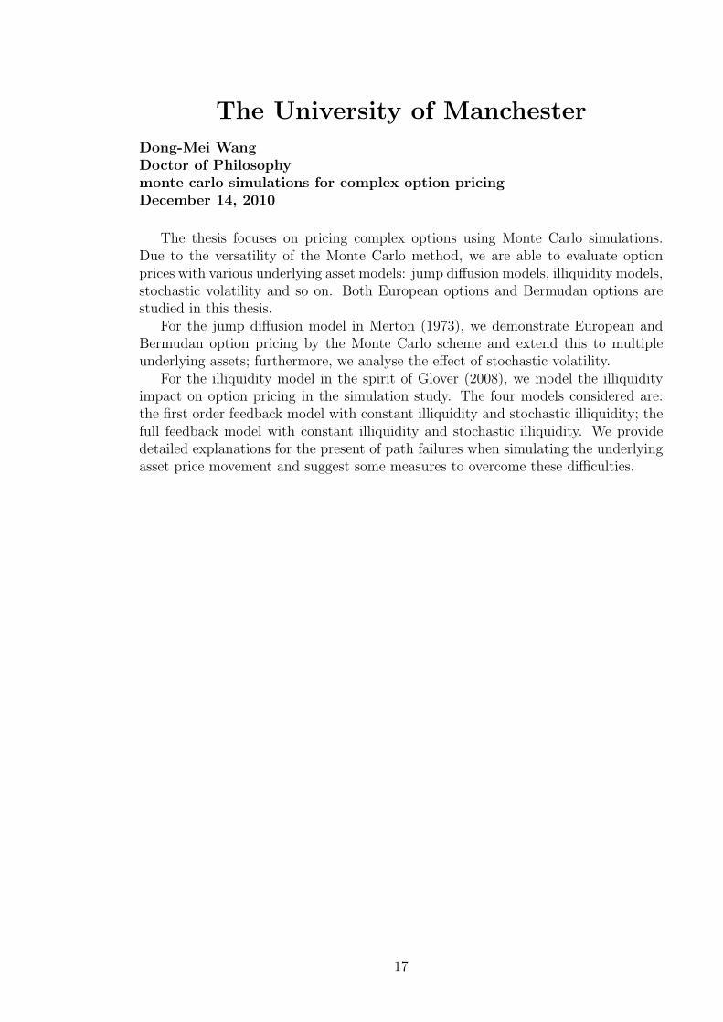
The thesis focuses on pricing complex options using Monte Carlo simulations.Due to the versatility of the Monte Carlo method, we are able to evaluate optionprices with various underlying asset models: jump diffusion models, illiquidity models,stochastic volatility and so on. Both European options and Bermudan options arestudied in this thesis.
For the jump diffusion model in Merton (1973), we demonstrate European andBermudan option pricing by the Monte Carlo scheme and extend this to multipleunderlying assets; furthermore, we analyse the effect of stochastic volatility.
For the illiquidity model in the spirit of Glover (2008), we model the illiquidityimpact on option pricing in the simulation study. The four models considered are:the first order feedback model with constant illiquidity and stochastic illiquidity; thefull feedback model with constant illiquidity and stochastic illiquidity. We providedetailed explanations for the present of path failures when simulating the underlyingasset price movement and suggest some measures to overcome these difficulties.
17

Declaration
No portion of the work referred to in this thesis has been
submitted in support of an application for another degree
or qualification of this or any other university or other
institute of learning.
18

Copyright Statement
i. The author of this thesis (including any appendices and/or schedules to this
thesis) owns any copyright in it (the “Copyright”) and s/he has given The
University of Manchester the right to use such Copyright for any administrative,
promotional, educational and/or teaching purposes.
ii. Copies of this thesis, either in full or in extracts, may be made only in accor-
dance with the regulations of the John Rylands University Library of Manch-
ester. Details of these regulations may be obtained from the Librarian. This
page must form part of any such copies made.
iii. The ownership of any patents, designs, trade marks and any and all other
intellectual property rights except for the Copyright (the “Intellectual Property
Rights”) and any reproductions of copyright works, for example graphs and
tables (“Reproductions”), which may be described in this thesis, may not be
owned by the author and may be owned by third parties. Such Intellectual
Property Rights and Reproductions cannot and must not be made available
for use without the prior written permission of the owner(s) of the relevant
Intellectual Property Rights and/or Reproductions.
iv. Further information on the conditions under which disclosure, publication and
exploitation of this thesis, the Copyright and any Intellectual Property Rights
and/or Reproductions described in it may take place is available from the Head
of the School of Mathematics.
19

Acknowledgements
I would like to express my sincere appreciation and gratitude to my supervisors Pro-
fessor Peter W. Duck and Professor David P. Newton for their helpful suggestions
and discussions throughout of my research. Without their support, collaboration and
guidance, I would not come to this stage along the way.
Also I would gratefully acknowledge the colleagues in Financial Mathematics Group
in University of Manchester for their generous help and advice. A special thanks to
Sebastian Law and Edwin Broni-Mensah in particular for their unwavering enthusi-
asm and encouragement.
Last, but by no means least, I am deeply indebted to my parents. Their love and
endless support gave me the energy to attain the study. This thesis is dedicated to
them.
20

Dedication
To Dad and Mom. . .
21

Chapter 1
Introduction
What is the last thing you do before you climb on a ladder? You shake
it, and that is Monte Carlo simulation.
– Sam Savage
Business Week, 22 January 2001
The enormous growth of derivatives markets since the 1970s has made option-
pricing theory one of the most dynamic areas in finance. It has become more im-
portant than before because many corporate liabilities can be expressed in terms of
options or combinations of options. In the absence of closed-form analytical solu-
tions of derivatives’ prices, numerical solution is required. For example, the pricing
of American, path-dependent and multi-asset options features, generally involves the
use of numerical methods. Aside from these relatively more complicated options,
it is also difficult to provide analytic solutions to European style options based on
underlying asset price models incorporating jumps in returns, jumps in volatility and
stochastic interest rates. Thus, pricing problems ultimately very often require a nu-
merical procedure, and the choice of methods involves the best combination of speed,
accuracy, simplicity and generality.
In a frictionless market, the arbitrage price of options can be expressed as the
expectation of the corresponding payoff, which is usually defined as a function of the
underlying asset price process. The founding papers in option pricing are Black and
22
CHAPTER 1. INTRODUCTION
Scholes (1973) and Merton (1973). Black and Scholes assume that the underlying
asset price follows a geometric Brownian motion and set up a replicating portfolio
which consists of an option and short a number of units of the underlying. A no
arbitrage argument leads to a second-order-linear partial differential equation (PDE)
determining the option values (the Black-Scholes-Merton PDE). Boundary conditions
are then applied, according to the option type and option pricing is achieved by
solving the PDE. The Black-Scholes formula can be viewed in terms of a risk-neutral
world, given that there is continuous hedging. This means that in such a world,
expected returns on the portfolio are equal to the risk-free rate of interest.
The present thesis focuses on Monte Carlo simulation to obtain numerical so-
lutions to option pricing problems. Monte Carlo simulation is a widely used tool
within finance for computing the price of financial instruments. Boyle (1977) first
proposed the application of Monte Carlo the technique to evaluate the value of Eu-
ropean options. Other pioneering works include Bossaerts (1989) and Tilley (1993).
The basic principle behind option pricing by the Monte Carlo method is to calculate
the expected value of a quantity which is a function of the solution to a stochastic
differential equation (SDE). Recent research focuses on: (1) path simulation methods,
especially when there are nonlinearities in the financial SDEs such as full feedback
models studied by Frey and Patie (2002); (2) computational improvements through
variance reduction techniques discussed in detail in Glasserman (2003); (3) extending
the Monte Carlo method to price complex financial derivatives, such as American op-
tions proposed in Longstaff and Schwartz (2001) and foreign exchange derivatives in
Xiao (2007). Extensive discussions on the development of Monte Carlo simulation for
option pricing are given by Boyle, Broadie and Glasserman (1997) and Glasserman
(2003). For a more comprehensive reference on analysis of numerical methods for
solving SDEs, see Kloeden and Platen (1999).
The Monte Carlo method has distinct advantages in dealing with a wide range
of option types because it is simple and flexible. The method is based on the dis-
tribution of terminal asset prices, determined by the process governing the future
price movements. The calculation generates a series of asset price trajectories and
23

CHAPTER 1. INTRODUCTION
the terminal asset prices from the series are used to estimate the option price and
compute the confidence limits at the same time. The standard error of the estimate
scales as 1/√n, where n denotes the number of the trajectories. Since this is inde-
pendent of the number of dimensions, the Monte Carlo method does not suffer from
the “curse of dimensionality” that affects other numerical techniques in finance. As
for the improvement of the efficiency, much attention has been put on quasi-Monte
Carlo and low-discrepancy methods (see Niederreiter, 1992; Birge, 1995; Paskov and
Traub, 1995; Joy, Boyle and Tan, 1996; Owen, 1997).
This thesis will focus on Monte Carlo simulations to solve option pricing problems
on particular underlying (complex) asset models, including jump diffusion models and
feedback models. The main contributions made in this thesis are stated as follows:
In the jump diffusion models, we calibrate the Merton (1976) model using an
analytical solution and compare the result with that of the Black-Scholes option
pricing formula. We also introduce another kind of jump diffusion model in this thesis,
which is called double-jump stochastic volatility model. Both models are extended
into multiple dimensional case to price basket options. The key contribution made
here is to illustrate a least square regression method of pricing Bermudan options
under these jump diffusion models. Numerical results show how the parameters of
specific models impact on pricing options. In addition, the simulation is accompanied
by an extrapolation technique to improve the accuracy.
The another main contribution of the thesis is to provide a numerical solution to
pricing options in feedback models, which are developed from Glover (2008), using
Monte Carlo simulation. We derive two kinds of the feedback models: the first-order
feedback and the full feedback models. The implementation of the first-order feedback
model is straightforward. However, there still exist a small amount of invalid sample
paths that have to be discarded. We give the reason to explain the phenomenon
and suggest to discard these paths from the simulation, under the assumption that
the law of large number holds. For the full feedback model, the implementation is
more complicate than that of the first-order feedback model. We use a three-point
finite difference method to compute the second partial derivatives of option prices
24

CHAPTER 1. INTRODUCTION
with respect to asset prices (i.e. Gamma). The Gammas are calculated at each
time step from the current simulated path, then we reproduce the same path using
these Gammas. The procedure continues iterating until a convergent option price is
obtained from the path. As the first-order feedback model, there are invalid sample
paths observed during the simulation. We propose several methods to reduce the
abandonment rate of the sample paths. One of them is that we price a call option
by the corresponding put option value with the put-call parity. This is because the
abandoned paths occur less frequently when pricing a put option than pricing a call
option. To obtain a convergent option price, we suggest to use a smoothed payoff
function instead of a standard payoff. But there exists a restriction of the smoothing
parameter. If the restriction did not satisfies, there would be a number of abandoned
paths during the simulation. The feedback models have been extended to include
a stochastic illiquidity process. An option price comparison of these four feedback
models is made in this thesis. For a long-term option,1 the model with the stochastic
illiquidity leads to a modest lower option price, compared with the constant illiquidity
model. The option price in the full feedback model is lower than that of the first-order
feedback model. A discussion of the corresponding implied volatilities are included
in this thesis.
In sum, we provide numerical solutions to pricing Bermudan options in the Mer-
ton jump diffusion model and the double-jump stochastic volatility model using
Monte Carlo simulation. With an extrapolation method, a desirable estimate can
be achieved. In feedback models, we concentrate on solving the difficulties in the
model implementation using Monte Carlo simulation. The thesis also presents nu-
merical results of parameter sensitivity in all models.
Chapter 2 provides a brief introduction to the fundamental principles underlying
Monte Carlo simulation and theorems of derivative pricing. A short review of various
techniques to improve the accuracy of the simulation pricing is presented, which
includes variance reduction methods, discretization methods and Quasi Monte Carlo
methods. Calculation of Greeks and American option pricing through simulation
1Normally, its maturity is longer than two years.
25

CHAPTER 1. INTRODUCTION
methods are discussed in this chapter.
In Chapter 3, we investigate the underlying asset process involving unpredictable
jump events. The basic jump diffusion model has been extended in two ways: turning
single asset cases into multiple asset cases and replacing a constant volatility with
a stochastic volatility. The correlations between asset returns and their volatilities
are also discussed. The examples covered in this chapter are arranged in increasing
order of complexity. We start with pricing one-dimensional Bermudan options with
constant volatility in Section 3.3, then consider pricing multi-dimensional options in
Section 3.4. In Section 3.5 and Section 3.6, we study underlying asset price processes
with jumps and stochastic volatility in one-dimensional and multi-dimensional cases,
respectively.
From Chapter 4 to Chapter 8, we focus on another kind of asset model, referred to
feedback models, which include the price impact of trade volume in an illiquid market
for the underlying. Chapter 4 gives an introduction to the model types and derives
two generalized forms of feedback model: first-order feedback and full-order feedback.
The former are discussed in Chapter 5 where the illiquidity is assumed to be constant
and Chapter 6 where stochastic illiquidity is employed; the latter are addressed in
the next two chapters: Chapter 7 focuses on the full feedback model with constant
illiquidity and Chapter 8 considers stochastic illiquidity.
Chapter 9 gives a summary of the thesis and several suggestions for further studies.
26
Chapter 2
Preliminaries
Anyone who considers arithmetical methods of producing random digits
is, of course, in a state of sin.
– John von Neumann
Various techniques used in connection with random digits, 1951
This chapter is arranged as follows. We address principles underlying derivative pric-
ing in Section 2.1 and Monte Carlo methods in Section 2.2. The core algorithm
of Monte Carlo methods is based on a uniform random number generator, which
is introduced in Section 2.3. To improve the Monte Carlo simulation, Section 2.4
discusses various variance reduction techniques and analyzes the advantages and dis-
advantages of the application of such methods. Section 2.5 presents several basic
discretization schemes to reduce the bias in Monte Carlo estimates. Section 2.6
develops an optimal strategy for allocation of computing time to reduce sampling
error and discretization error in the simulation. The implementation of Monte Carlo
methods for the evaluation of the Greeks is introduced in Section 2.8 and a numerical
example is illustrated to show that Monte Carlo estimates converge towards the cor-
responding exact values calculated by the Black-Scholes formula (the exact solution
of the Black-Scholes-Merton PDE for plain European options). Section 2.9 presents
several modified Monte Carlo simulations to deal with pricing American options.
27
CHAPTER 2. PRELIMINARIES
2.1 Principles of derivatives pricing
Kwok (2008, p. 35) states that “The concepts of replicable contingent claims, absence
of arbitrage and risk neutrality form the cornerstones of modern option pricing the-
ory.” In this section, basic mathematical concepts underlying derivative pricing are
presented, with important applications of Monte Carlo methodology.
2.1.1 Arbitrage pricing
One of the basic requirements of (financial) derivatives pricing is the no-arbitrage
principle. The absence of arbitrage opportunities brings to mind the common expres-
sion “there’s no such thing as a free lunch”. More formally, an arbitrage can arise in
either of the following scenarios (see Glasserman, 2003):
1. θ(0)>S(0) < 0 and P(θ(t)>S(t) ≥ 0
)= 1;
2. θ(0)>S(0) = 0 and P(θ(t)>S(t) ≥ 0
)= 1, and P
(θ(t)>S(t) > 0
) ≥ 0;
where P represents the true (objective) probability measure in the real world; S(t)
represents the current state of d assets at time t, i.e. S(t) =(S1(t), · · · , Sd(t)
)>;
θ(t) =(θ1(t), · · · , θd(t)
)is the number of units of each asset held at time t, which is a
self-financing trading strategy1. The first statement (1) describes that one can follow
the trading strategy with a negative current net commitment that yet produces a
positive profit in the future. The second trading strategy (2) without net investment
today can guarantee a nonnegative final wealth. Both strategies lead to arbitrage
opportunities to create an excess profit that contradicts the existence of economic
equilibrium. In practice, arbitrage opportunities may exist during short intervals;
however these mispricings will be corrected by the pressure of supply and demand
in the market. The no-arbitrage argument is one of the fundamental assumptions
in deriving the celebrated Black-Scholes-Merton partial differential equation (see for
example Wilmott, Howison and Dewynne, 1995).
1A trading strategy is self-financing if it satisfies θ(t)>S(t)− θ(0)>S(0) =∫ t
0θ(u)>dS(u) .
28
CHAPTER 2. PRELIMINARIES
2.1.2 Risk-neutral probabilities
A risk-neutral probability, which we denote by Q, is a synthetic probability cor-
responding to P, meaning that they have the same set of zero probability. The
fundamental theorem of asset pricing states that in the absence of arbitrage opportu-
nities in a complete market implies that there exists a unique equivalent risk-neutral
measure (e.g. Kwok, 2008). Hence, under the risk-neutral measure, the valuation
of an option is given by the expected payoff of the option discounted by a risk-free
rate rather than the real (time varying) rate for the underlying asset. For example,
consider the price of the i-th of d assets following a system of SDEs:
dSi(t)
Si(t)= µidt+ σ>i dW P(t) ,
where µi is the drift parameter reflecting investor attitudes towards risk: she may
expect to risker assets to win a higher return; σi is the diffusion parameter andW P is a
Brownian motion under the objective measure P. The relative risk-neutral dynamics
of the asset prices can be described as:
dSi(t)
Si(t)= rdt+ σ>i dWQ(t) ,
with a riskless growth rate r and a different Brownian motion WQ under the risk-
neutral measure Q. Comparing the two systems of SDEs, we find the relation between
W P and WQ, which is:
dWQ(t) = dW P(t) + ν(t)dt ,
for some ν(t) satisfying
µi = r + σ>i ν , i = 1, · · · , d .
This presentation suggests that ν(t) can be interpreted as a risk premium, which is
an additional return from the risky asset over that from a risk-free asset. ν is also
called the market price of risk. There are advantages in using Q measure over the P
measure for Monte Carlo simulation:
29
CHAPTER 2. PRELIMINARIES
• It is easier to produce sample paths with a risk-free rate r under risk-neutral
measure. Because under the real probability measure P, the drift parameter µi
associated with varying risk preferences of investors is much harder to estimate,
while r can be estimated as a riskless interest rate.
• The option price can be estimated as the expected payoff at expiry discounted
at a risk-free rate, namely,
V (t) = e−r(T−t)EQ(V (T )) , t < T ,
where EQ is the expectation under the risk-neutral measure Q. This also implies
that the price process V (t) is a Q-martingale as the expected discounted value
of e−r(T−t)V (T ) does not change with time and is equal to the current value
V (t).
2.2 Principles of Monte Carlo
In this section, some fundamental theorems of probability and statistics applied to
the Monte Carlo techniques will be introduced. The definition and results reviewed
in this section can help readers understand what principles support the numerical
method.
When we analyse a method, there are three particularly important considerations:
bias, variance and computing time.
2.2.1 Law of large numbers
Consider the case of a general random variable X, whose expected value E(X) = µ
and variance V ar(X) = σ2 are not known. If we let X1, X2, . . . , Xn denote indepen-
dent random variables with the same distribution as X, then we might expect the
estimator µ
µ :=1
n
n∑i=1
Xi (2.1)
30

CHAPTER 2. PRELIMINARIES
E(µ) =1
n{E(X1) + E(X2) + · · ·+ E(Xn)}
=1
n{µ+ µ+ · · ·+ µ}
= µ
to be a good approximation to µ. This is a unbiased estimator, that is, its expected
value is the same as µ. The detailed definition is given as follows.
Theorem 2.1 (Law of Large Numbers). Let X1, X2, . . . , Xn be an independent
trials process, with finite expected value µ = E(Xi) and finite variance σ2 = V ar(Xi).
Let Sn = X1 +X2 + . . .+Xn, then for any ε > 0,
P (|Sn
n− µ| ≤ ε) → 0 as n→∞.
Equivalently,
P (|Sn
n− µ| < ε) → 1 as n→∞.
In fact, the law of large numbers ensures that this estimate µ converges to the correct
value, µ, as the number of random variables increases. This idea leads us to the basic
Monte Carlo method for approximating the expectation of a function of a random
variable. We take a long run average of the function as its expectation. Using a
similar method, one can estimate the variance σ2 using the sample variance σ2 as
follows (Miller and Miller, 2004):
σ2 :=1
n− 1Σn
i=1(Xi − µ)2 . (2.2)
E(σ2) = E(1
n− 1Σn
i=1(Xi − µ)2)
=1
n− 1E(Σn
i=1(X2i − 2µXi + µ2))
=1
n− 1{E(Σn
i=1X2i )− E(Σn
i=12µXi) + E(Σni=1µ
2)}
=1
n− 1(E(Σn
i=1X2i )− E(nµ2))
=1
n− 1(nE(X2
i )− nE(µ2)) ,
31

CHAPTER 2. PRELIMINARIES
since E(µ2) = V ar(µ) + E2(µ)
=σ2
n+ µ2 ,
thus E(σ2) =1
n− 1[n(σ2 + µ2)− n(
σ2
n+ µ2)]
= σ2 ,
which shows that σ2 is an appropriate unbiased estimate of σ2.
2.2.2 Central limit theorem
Now we are interested in the difference between µ and µ, that is µ − µ. First we
introduce the Central Limit Theorem which is the second foundational theorem in
probability.
Theorem 2.2 (Central Limit Theorem). Let X1, X2, . . . , Xn be a sequence of
i.i.d. random variables with expectation µ and variance σ2, then the distribution of
µ− µ ∼ N(0,σ2
n)
as n −→∞, where µ = 1n
∑ni=1Xi. Equivalently,
µ− µσ√n
∼ N(0, 1)
as n −→∞.
This suggests that if the sample size n is very large, the estimate µ should be
close to µ, with error O( 1√n).
We can make the argument more precise by using the idea of a confidence interval.
By applying the unbiased estimators µ in (2.1) and σ2 in (2.2), the confidence interval
for the estimate µ with probability 0.95 can be gained from
P(| µ− µσ√n
| ≤ 1.96) = 0.95
P(µ− 1.96σ√n
≤ µ ≤ µ+1.96σ√
n) = 0.95
that is,
[µ− 1.96σ√n, µ+
1.96σ√n
] . (2.3)
32

CHAPTER 2. PRELIMINARIES
This interval ensures the efficiency of the Monte Carlo method to approximate µ. In
100.3
100.2
100.1
100
101 102 103 104 105 106
Sam
ple
mea
n
Num samples
Figure 2.1: Monte Carlo approximation to E(eZ), where Z ∼ N(0, 1). Vertical linesgive computed 95% confidence intervals, middle points on the vertical lines are theapproximations. Horizontal dashed line is at height E(eZ) =
√e.
Figure 2.1 we give results from a Monte Carlo simulation of E(eZ), where Z ∼ N(0, 1).
In this case, we used 13 different sample sizes, n = 25, 26, . . . , 217. For each sample,
the picture plots the computed mean µ with circles and 95% confidence interval
with vertical lines. Compared with the theoretical expection2 of eZ , we see as the
sample size n increases the computed mean becomes more accurate and the confidence
interval shrinks.
There are two points to note:
• The size of confidence interval reduces slowly. In fact, to reduce the error by
0.1, the number of sample n has to increase by 100. The stated estimation error
is O( 1√n).
• It is required that n is sufficiently large so that the Central Limit Theorem
approximation is accurate.
2If Z is a normal random variable with mean a and volatility b, then Y = eZ has a log-normaldistribution with mean ea+ 1
2 b and volatility (eb2 − 1)e2a+b2 .
33

CHAPTER 2. PRELIMINARIES
2.3 Generating random numbers
In this section we briefly introduce algorithms at the core of Monte Carlo simula-
tion methods for generating uniformly distributed random numbers and transforming
them into a normal distribution. This algorithm may be run a million times for a
single valuation, so its efficiency will be important.
• Linear Congruential Generator
The general linear congruential generator, firstly proposed by Lehmer (1951),
has the form
xi+1 = (axi + c) mod m
ui+1 = xi+1/m
for some integers a, m and c (although it is now customary to take c = 0). For
each i = 1, 2, · · · , xi is generated by an iterative process given an initial value
x0 as ‘seed’ chosen from (0,m), and the resulting values ui always lie in the
unit interval. Bratley, Fox and Schrage (1987) show a faster implementation of
a linear congruential generator using only integer arithmetic and still avoiding
overflow. Let
q = bm/ac, r = m mod a
so that
axi mod m = a(xi mod q)− bxi
qcr + (bxi
qc − baxi
mc)m .
We can show (bxi
qc − baxi
mc) only takes the values 0 and 1. This means that
now the modular operator is only required by xi, which can implemented faster
than the calculation of axi mod m. See a detailed discussion of the linear
congruential generator in Glasserman (2003).
• Transformation Method: Normal Random Numbers
In the previous section, we saw how to generate random numbers with a uniform
distribution. Now we introduce the Box-Muller (1958) method, which is the
simplest technique for generating Normally distributed random numbers by
34

CHAPTER 2. PRELIMINARIES
taking any uniformly distribution variables. Given two uniformly distributed
random numbers x1, x2, two Normally distributed random numbers, y1 and y2
are given by:
y1 = cos(2πx2)√−2 log x1
y2 = sin(2πx1)√−2 log x2
2.4 Variance reduction techniques
One of the drawbacks of the Monte Carlo method arises from the slow decrease of
error, at a rate inversely proportional to the square root of the number of simulations.
Although any desired precision can be obtained by increasing the simulation trails,
it is useful to provide more efficient ways to reduce error.
2.4.1 Control variates
One method to improve accuracy is known as the control variate approach. To
compute the expectation E[X] of random variable X, we can estimate it through
another independent random variable Y , satisfying the following conditions:
• the random variable Y has a known mean µ,
• and there is a strong correlation between the random variables X and Y .
Then, we generate random variable X rather than X,
X = X − Y + µ,
and estimate the expectation E[X] = 1n
∑ni=0 X. This is because X is an unbiased
estimate of X, i.e.
E[X] = E[X]− E[Y ] + µ = E[X] ,
but with lower variance than the original X, that is
V ar[X] = V ar[X] + V ar[Y ]− 2ρXY
√V ar[X]V ar[Y ]
< V ar[X] ,
35

CHAPTER 2. PRELIMINARIES
where the correlation ρXY > 12
√V ar[Y ]V ar[X]
, which is implied by the second condition of
Y . One of typical examples is to compute an arithmetic average price Asian call
option with payoff X:
max
[1
n
n∑i=1
S(ti)−K, 0
].
Let Y be the corresponding geometric average price Asian option with payoff
max
[1
n
n∏i=1
S(ti)−K, 0
],
then the expectation E[Y ] has an explicit formula assuming S(ti) follows a standard
Brownian motion with constant drift and variance terms. Therefore, we may use
Y as a control variate to estimate E[X]. There are some other typical examples
shown in Bolia and Juneja (2005), such as the European option pricing problem on
a dividend paying stock. The control variates method is discussed in more detail
and extended to multiple controls in Glasserman (2003). Rasmussen (2005) develops
pricing American options using control variates.
2.4.2 Antithetic variates
Another method to improve convergence is through the use of antithetic variates. This
produces antithetic pairs of random numbers, U and 1−U from a uniform distribution,
which ensures that the random numbers are symmetrically distributed with mean
zero so that the variance from asymmetric sampling in the original simulation has
been reduced. The implementation is straightforward: we generate a path with N
standard normal random variables Zi, and then directly gain another path with −Zi
for i = 0 . . . N − 1 which moves in the opposite direction. Both control variates
and antithetic variates techniques are described in the paper by Boyle (1977). In
the case of European options on discrete dividend-paying stock, Bolia and Juneja
(2005) show that the use of both methods, antithetic variates and control variates,
can considerably improve the accuracy of the estimators and shrink the confidence
interval.
36
CHAPTER 2. PRELIMINARIES
2.4.3 Importance sampling
Importance sampling (see Glasserman, 2003) is a popular method of variance re-
duction, with emphasis on generating important sample paths for the corresponding
options. For example, consider a European call option with strike price K, which is
deep out of the money (S(0) << K). In such a situation, the accuracy of a standard
Monte Carlo method suffers because most of the simulated sample paths expire out
of the money and also some rare but large big payoffs could be missed. However,
we can use importance sampling to generate important paths, that is S(T ) > K.
Assume that r.v. X follows the probability density function (pdf) f(x), there exists
another pdf g(x), the expectation of X can be estimated as:
E[X] =
∫ ∞
−∞xf(x)dx
=
∫ ∞
−∞xf(x)
g(x)g(x)dx
=
∫ ∞
−∞xW (x)g(x)dx (2.4)
= E[XW (X)] ,
where w(x) = f(x)g(x)
is a likelihood ratio and is referred to as the weighting function.
The third equality (2.4) implies a change of probability measure from f(x) to g(x),
and E(·) is the expectation under g(x). Therefore, we can draw random variable X
from g(x) and convert it to the estimator XW (X) which is unbiased to the estimator
X from f(x). To continue with the above example, the sample paths are simulated
with the random increments from a specific uniform distribution U [a, b] (rather than
the standard uniform distribution U [0, 1]) such that S(T ) > K. Then we compute
the expectation of option price multiplied by their weighting W (x) = b − a. The
variance of importance sampling is simply given by:
V ar[XW (X)] = E[X2W (X)2]− E2[XW (X)]
= E[X2W (X)2]− E2[X]
= E[X2W (X)]− E2[X] , (2.5)
37
CHAPTER 2. PRELIMINARIES
whilst the naive Monte Carlo method has the variance:
V ar[X] = E[X2]− E2[X] . (2.6)
From Eq (2.5), zero variance can be obtained when W (X) = E[X]X
, however, E[X]
is unknown a priori. Comparing the two variances in Eq (2.5) and Eq (2.6), we can
see that importance sampling reduces the variance when W (X) < 1, otherwise, it
could also increase the variance. Consider our example again, W (X) is constant and
equals b−a. From the analytical solution of underlying S(t), we infer that b = 1 and
a > 0 so that W (X) < 1, i.e. V ar[XW (X)] < V ar[X], which shows that importance
sampling gives a better estimator with lower variance over the naive Monte Carlo
method. An optimal choice of the probability density function g(x) should minimize
variance, which is the key to the efficiency of importance sampling. Bolia and Juneja
(2005) and Glasserman (2003) illustrate this problem with different examples, such
as one-dimensional up-and-in European put options and Bermudan options. Guasoni
and Robertson (2008) derive an optimal change of drift terms for pricing Asian op-
tions, and show that importance sampling greatly improves the performance of the
Monte Carlo method. In the standard Black-Scholes model, for both geometric and
arithmetic average Asian options, the closed form explicit formulae of the change of
drift are obtained by solving the corresponding Euler-Lagrange equation, which is
a differential equation whose solution is the stationary value of a given functional.
Their basic idea is to solve a variational problem u Their paper is based on Glasser-
man, Heidelberger and Shahabuddin’s (1999) work and extends it to a continuous
time framework.
Besides the methods above, a number of effective techniques have been developed
to reduce the variance of the estimates in Monte Carlo applications, such as moment
matching and stratified sampling, which are described in detail by Glasserman (2003),
Bratley et al. (1987) and Law and Kelton (1991).
38
CHAPTER 2. PRELIMINARIES
2.5 Discretization methods
In this section, we will introduce discretization methods for the simulation of a
stochastic process and demonstrate the convergence rate of the error.
2.5.1 The Euler method
The Euler method (Higham, 2004) is an explicit numerical method for approximating
the solution of a stochastic differential equation, which is based on the idea of the Ito
stochastic integral (El-Borai, El-Nadi, Mostafa and Ahmed, 2005) as in the following:
∫ T
t=0
f(t,W (t))dW (t) = limN→∞
N∑i=1
f(ti,W (ti))(W (ti)−W (ti−1)) ,
whereWt is a Brownian motion and N is defined as a finite number of shorter intervals
of length ∆t = T/N in the whole interval [0, T ].
We assume a stochastic process X(t) is the solution to the following generalised
stochastic differential equation, which is
dX(t) = f(X(t))dt+ g(X(t))dW (t) , 0 ≤ t ≤ T, (2.7)
where f(X(t)) and g(X(t)) are given functions of the stochastic process X(t). Given
the length of the interval T , the time step size ∆t = T/N for some positive integer
N , and ti = ti−1 + ∆t for i = 1, · · · , N , by integrating both sides of (2.7) from ti−1
to ti, we can rewrite the stochastic differential equation in integral form as
X(ti) = X(ti−1) +
∫ ti
ti−1
f(X(s))ds+
∫ ti
ti−1
g(X(s))dW (s) , (2.8)
which is the exact solution X(ti). Approximations Xi for X(ti) using the Euler
method can be expressed as:
Xi = Xi−1 + f(Xi−1)∆t+ g(Xi−1)(W (ti)−W (ti−1))
= Xi−1 + f(Xi−1)∆t+ g(Xi−1)√
∆tZi−1 , (2.9)
where Zi−1 is a normal random variable with mean 0 and variance 1 due to the basic
properties of the Brownian motion W (t). The approximation Xi approaches X(ti)
from the exact solution (2.8) as ∆t reduces to zero.
39
CHAPTER 2. PRELIMINARIES
There are many different, non-equivalent, definitions of convergence for sequences
of random variables. The two most common and useful concepts in numerical stochas-
tic differential equations are strong convergence and weak convergence, which are
defined in Higham (2004) as follows:
A method is said to have strong order of convergence equal to p if
there exists a constant C such that
E|Xi −X(ti)| ≤ C∆tp ,
for sufficiently small ∆t; similarly, a method has a weak order of p if there
exists a constant C such that
|EXi − EX(ti)| ≤ C∆tp ,
where E denotes the expected value.
In other words, the strong convergence is a convergence of the mean of the error
and the weak convergence is convergence of the error of the mean. A discretization
scheme normally has a lower strong order than the weak order. For the study of
option pricing, the weak convergence is more relevant than the strong convergence,
because we are interested in the difference between the estimate EXi and the exact
value X(ti). As shown in Higham (2004), the Euler method typically has a strong
order of 1/2 but it can achieve a weak order of 1.
2.5.2 The Milstein method
From a Taylor expansion, we can find that the approximation (2.9) expands the drift
term to O(∆t) whilst the diffusion term up to O(√
∆t). The Milstein (1975) method
is derived through expanding the diffusion term to O(∆t), being of the same order
of the drift term. The approximation given by the Milstein method is in the form:
Xi = Xi−1 + f(Xi−1)∆t+ g(Xi−1)√
∆tZ(ti−1)
+1
2g′(Xi−1)g(Xi−1)∆t(Z
2i−1 − 1) . (2.10)
40
CHAPTER 2. PRELIMINARIES
Compared with the Euler method (2.9), the Milstein method adds the extra term
12g′(Xi−1)g(Xi−1)∆t(Z
2i−1 − 1), which requires that g(X) is a smooth function (i.e.
has a first derivative). Theorem 10.3.05 of Kloeden and Platen (1999) shows the
Milstein method has strong order 1, which is higher than the strong order 1/2 of the
Euler method. Higham (2001) provides a numerical test to compare the convergence
orders of the Milstein method and the Euler method.
2.5.3 The second-order Milstein method
The second-order method proposed by Milstein (1979) can improve the accuracy
of the approximation to converge weakly at O(∆t2). Consider the exact solution
(2.8), using Ito’s formula (Ito, 1951) to derive a exact representation for f(X(s)) and
g(X(s)) with s ∈ [t, t+ ∆t], which is
f(X(s)) = f(X(t)) +
∫ s
t
(ff ′ +1
2g2f ′′)du+
∫ s
t
gf ′dW (u) ,
g(X(s)) = g(X(t)) +
∫ s
t
(fg′ +1
2g2g′′)du+
∫ s
t
gg′dW (u) ,
where u ∈ [t, s]. We can see that the Euler method only approximates f(X(s)) ≈f(X(t)) and g(X(s)) ≈ g(X(t)) by ignoring the integral terms. However, the second-
order method approximates the values of two integral terms to produce a better
approximation of f(X(s)) and g(X(s)), which is
f(X(s)) ≈ f(X(t)) +{f(X(t))f ′(X(t)) +
1
2g2(X(t))f ′′(X(t))
} ∫ s
t
du
+g(X(t))f ′(X(t))
∫ s
t
dW (u) ,
g(X(s)) ≈ g(X(t)) +{f(X(t))g′(X(t)) +
1
2g2(X(t))g(X(t))′′
} ∫ s
t
du
+g(X(t))g′(X(t))
∫ s
t
dW (u) .
Substituting these two approximations to the first term and the second term of inte-
gral in (2.8):
X(t+ ∆t) ≈ X(t) + f(X(t))∆t+ g(X(t))∆t
+{f(X(t))f ′(X(t)) +
1
2g2(X(t))f ′′(X(t))
} ∫ t+∆t
t
∫ s
t
duds
41

CHAPTER 2. PRELIMINARIES
+{g(X(t))f ′(X(t))
} ∫ t+∆t
t
∫ s
t
dW (u)ds
+{f(X(t))g′(X(t)) +
1
2g2(X(t))g′′(X(t))
} ∫ t+∆t
t
∫ s
t
dudW (s)
+{g(X(t))g′(X(t))
} ∫ t+∆t
t
∫ s
t
dW (u)dW (s) ,
where double integrals can be resolved using stochastic calculus.∫ t+∆t
t
∫ s
t
duds =
∫ t+∆t
t
(s− t) ds =1
2∆t2 ,
∫ t+∆t
t
∫ s
t
dW (u)ds =
∫ t+∆t
t
(W (s)−W (t)) ds =1
2∆t∆W ,
∫ t+∆t
t
∫ s
t
dudW (s) =
∫ t+∆t
t
(s− t) dW (s) =1
2∆t∆W,
∫ t+∆t
t
∫ s
t
dW (u)dW (s) =
∫ t+∆t
t
(W (s)−W (t)) dW (s) =1
2∆W 2 − 1
2∆t ,
where ∆W = W (t+ ∆t)−W (t). Then, we can obtain the approximation X(t+ ∆t)
of Xi as follows:
Xi = Xi−1 + f(Xi−1)∆t+ g(Xi−1)∆W
+1
2
{f(Xi−1)f
′(Xi−1) +1
2g2(Xi−1)f
′′(Xi−1)}
∆t2
+1
2
{g(Xi−1)f
′(Xi−1) + f(Xi−1)g′(Xi−1) +
1
2g2(Xi−1)g
′′(Xi−1)}
∆t∆W
+1
2
{g(Xi−1)g
′(Xi−1)}
(∆W 2 −∆t) ,
where ∆W is normally distributed with mean 0 and variance ∆t; coefficient function
f , g and their derivatives are evaluated at Xi−1.
Talay (1984) and Kloeden and Platen (1999) have shown that this scheme has
a weak convergence order of 2. Moreover, the method can be extended to deal
with a high-dimensional problem, which is discussed in Talay and Tubaro (1990)
and Glasserman (2003). However, the second-order method requires smooth coeffi-
cient functions and calculation of the derivatives of the coefficient functions at each
timestep, which increases the complexity of simulation, especially for those prob-
lems whose derivatives have to been estimated by numerical methods, such as finite-
difference approximations. Therefore, there is an increase in the calculation time of
simulation for each sample path, so the second-order method is usually slower than
the Euler method.
42
CHAPTER 2. PRELIMINARIES
2.5.4 The extrapolation method
The extrapolation method is described in Glasserman (2003) as an alternative ap-
proach to achieve a weak convergence O(∆t2) using two estimates, which are calcu-
lated by the first-order convergence rate with different level timestep ∆t, to extrap-
olate the more accurate estimate. The method is far easier to implement than the
second-order method described previously. As the standard Euler method has weak
order 1, Talay and Tubaro (1990) show that the relation between estimate Xi for and
the exact value X(ti) can be expressed as:
EX(∆t)i = EX(ti) + C∆t+O(∆t2) ,
EX(2∆t)i = EX(ti) + 2C∆t+O(∆t2) ,
where C is the same constant in both cases; X(∆t)i represents the approximation using
timestep ∆t and X(2∆t)i is gained by setting timestep 2∆t. By combining these two
estimates, we can obtain an extrapolated estimate, that is
2EX(∆t)i − EX(2∆t)
i = EX(ti) +O(∆t2) , (2.11)
which has weak order of 2. This means that the combining estimate is more accurate
than either of its two components. In fact, the extrapolation method can be applied
to further increase the convergence order, which is discussed in Glasserman (2003).
We have introduced several basic discretization schemes in this section. In gen-
eral, the extrapolation method is seen to have distinct advantages over the other
methods in that it is easy to implement and relatively efficient. There are still many
discretization methods which are derived from these basic schemes (see Kloeden and
Platen, 1999). We suggest that an efficient method chosen for simulation depends
on the specific features of the model we study. Sometimes even a simple change of
variable X(t) can help to reduce the bias during the simulation, such as replacing un-
derlying prices with the logarithm of the prices, which will be illustrated to simulate
a jump diffusion process in Chapter 3.
43
CHAPTER 2. PRELIMINARIES
2.6 Efficient Monte Carlo methods
As discussed in Section 2.4 and Section 2.5, Monte Carlo methods usually suffer error
from the number of simulations M and the length of time intervals ∆t. Under certain
conditions on f(x) and g(x) (see Talay and Tubaro, 1990; Kloeden and Platen, 1999),
it is well known that the sample mean-squared error3 (MSE) of the estimate given by
the Monte Carlo simulation associated with the Euler discretization is asymptotically
of the form
MSE ≈ C1M−1 + C2∆t
2 (2.12)
for positive constant C1 and C2. The first term represents the variance from sampling,
and the second term is due to the squared bias of the Euler method with weak order
1. A more general form of MSE is given by Glasserman (2003), which is:
MSE ≈ C1M−1 + C2∆t
2p . (2.13)
Then an efficient Monte Carlo method is considered to minimize the value of the
MSE (2.13).
With a limited budget of computation time, we have to consider how to make an
efficient tradeoff between reducing the size of timesteps ∆t and increasing the number
of sample paths M . The total computation time s is roughly proportional to M/∆t,
i.e. s ∝ M∆t
, meaning the number of discrete time steps for total sample paths, thus
the size of M/∆t is important. Duffie and Glynn (1995) show that an optimum root
mean square error4 (minimum RMSE) is gained by setting:
M ∝ ∆t−2p , (2.14)
then the minimum RSME is
RMSE ∝ s−p
2p+1 ,
where the magnitude of RMSE is reduced when the convergence order p increases
and tends to s−12 as p → ∞. The expression (2.14) suggests that for the first-order
3MSE(X) = E[(X −X)2] where X is an estimator of X.4RMSE(X) =
√MSE(X).
44

CHAPTER 2. PRELIMINARIES
Euler method p = 1, when we reduce ∆t by half, the number of sample paths should
be quadrupled; for the second-order scheme p = 2, the number of sample paths
is increased by a factor of 24. They also illustrate several option pricing examples
to show that the error reduction is somewhat halved using doubling the number of
timesteps each time for the Euler method and the error is reduced by a factor of
approximately 4 for the second-order method.
2.7 Quasi-Monte Carlo method
In contrast with ordinary Monte Carlo methods that compute an integral based
on sequences of pseudo random numbers, quasi-Monte Carlo (QMC) methods take
advantage of determined sequences with low discrepancy5, so the methods are also
known as low-discrepancy methods. The famous advantage of the QMC methods
is to achieve accuracy O(1/N) (N is the number of sample paths) which is higher
than the accuracy O(1/√N) associated with the normal Monte Carlo simulation.
However, this clever method has been found to suffer a problem of dimensionality.
By the Koksma-Hlawka inequality (see Glasserman, 2003), the integration error
for the QMC method over d-dimensional space is bounded by
∣∣∣∣1
N
N∑i=1
f(xi)−∫
[0,1]df(x)dx
∣∣∣∣ ≤ V ar(f)D∗(x1, x2, · · · , xN) ,
where V ar(f) is a bounded variation of function f(x) and D∗(x1, x2, · · · , xN) is the
discrepancy of the sequence. We can see the error of integration depends on the
product of the term of the function variation and the term of the discrepancy of the
sequence. As the variance is bounded, a low-discrepancy sequence results in a good
approximation of the integration.
For one-dimensional problems, Glasserman (2003) suggests taking base-b Van der
5Discrepancy is a measure of deviation from uniform distribution.
45

CHAPTER 2. PRELIMINARIES
Corput sequences stated in Van Der Corput (1935), which is defined as:
k =∞∑
j=0
aj(k)bj ,
ψb(k) =∞∑
j=0
aj(k)
bj+1, (2.15)
where k is a positive integer, aj(k) is the coefficient with respect to the power j
of the base b, ψb(k) is called as the radical inverse function to map k to a point in
interval [0, 1). Note that the sum in (2.15) has a finite number of non-zero terms. The
calculation of base-2 and base-3 sequences is illustrated in Table 2.1. The second
k k Binary ψ2(k) ψ3(k)0 0 0 01 1 1/2 1/32 10 1/4 2/33 11 3/4 1/94 100 1/8 4/95 101 5/8 7/96 110 3/8 2/97 111 7/8 5/98 1000 1/16 8/99 1001 9/16 1/27...
......
...
Table 2.1: Illustration of radical inverse function ψ2(k) and ψ3(k)
column ‘k Binary’ represents numeric values on base-2, which can be expressed in
the form of ajmaxajmax−1 · · · a1a0. The basic idea of the sequence is to ‘fill the gap’
between existing values. For example, given 0 and 1/2, we take the median value
between them as the next number for the base-2 sequence, that is 1/4. The van der
Corput sequences have been extended to generate d-dimensional sequences by Halton
(1960), which is :
xr = (ψb1(k), ψb2(k), · · · , ψbd(k)) ,
where ψb is given by Eq (2.15) and bi is chosen as the first i-th prime number, for
k = 0, 1, 2, · · · . For example, using the results in Table 2.1, we can construct a simple
46

CHAPTER 2. PRELIMINARIES
two-dimensional Halton sequence, which is
(0, 0), (1/2, 1/3), (1/4, 2/3), (3/4, 1/9), (1/8, 4/9), (5/8, 7/9),
(3/8, 2/9), (7/8, 5/9), (1/16, 8/9), (9/16, 1/27), · · ·
The smaller primes taken as a base usually perform better than the larger ones so
that for d-dimensional problem, we take the first d primes, such as 2, 3, 5 · · · . In fact,
there is a significant decline in uniformity of Halton sequences with increasing dimen-
sion, because large primes have to been chosen for high-dimensional problems. Thus,
other competitive methods are developed to construct the low discrepancy sequences
in multi-dimensional space, most commonly, such as Faure and Sobol sequences (see
more details in Glasserman, 2003). The basic idea for both sequences is to form a
finer uniform partition of the unit interval [0, 1] and reorder them for each dimension.
In contrast with different primes used as bases in Halton sequences, Faure sequences
use a common base that is the smallest prime number greater or equal to the dimen-
sion itself, and multi-dimensional Sobol sequences only use base 2. Thus, with equal
dimension, the bases used for these two methods are much smaller than the largest
base used to construct Helton sequences. More specifically, a Faure sequence is con-
structed by permuting a Van der Corput sequence multiplied by different dimension
itself. For each integer k, the expansion of base b is in the form:
k =r∑
l=0
al(k)bl .
Suppose there are r terms in the expansion of k, the point in i-th coordinate with
i = 1, 2, · · · , d can be found from:
ψ(i)b (k) =
∞∑j=1
y(i)j (k)
bj+1,
y(i)j (k) =
∞∑
l=0
(l
j − 1
)(i− 1)l−j+1al(k) mod b ,
where the summands vanish when l ≥ r as al(k) = 0, then we only need consider
the case of l < r; the combination(
lj−1
)is restricted by l ≥ j − 1 otherwise zero.
This implies that both sums have a finite number of terms. The term y(i)j (k) can be
47

CHAPTER 2. PRELIMINARIES
generated by the matrix-vector calculation, which is:
y(i)1 (k)
y(i)2 (k)
...
y(i)r (k)
= C(i−1)
a0(k)
a1(k)
...
ar−1(k)
mod b ,
where the matrix C(i) is a r × r generator matrix in the form:
C(i) =
(00
)i0
(10
)i1
(20
)i2 · · · (
r−10
)ir−1
0(11
)i0
(21
)i1 · · · (
r−11
)ir−2
0 0(22
)i0 · · · (
r−12
)ir−3
......
... · · · ...
0 0 0 · · · (r−1r−1
)i0
,
and the generator matrix can be obtained using a recursive equation:
C(i) = C(1)C(i−1) ,
for any i = 1, 2, · · · , d.Now we turn to discuss an alternative method introduced by Sobol (1967). The
Sobol sequence is constructed in a similar way as the Faure one by multiplying gener-
ator matrices by a vector of coefficients of a binary expansion of k, i.e. in base 2–the
smallest prime number, which implies that it costs less computation time to generate
the Sobol sequences than the Faure sequences with equal dimension. The key dif-
ference between two low discrepancy sequences is the construction of the generator
matrices. For the Sobol sequence, the generator matrix is separately constructed
by a primitive polynomial for each coordinate i, i = 1, 2, · · · , d. Paskov and Traub
(1995) first propose the QMC method with Halton and Sobol sequences to price a
collateralized mortgage obligation (CMO) and show that the QMC method is su-
perior to the regular Monte Carlo method. As suggested in Glasserman (2003), the
Sobol sequences always produce results more accurately and quickly than other QMC
sequence and Monte Carlo methods. The combination of the Sobol points with the
Brownian bridge6 construction is recommended.
6A Brownian bridge is a stochastic process B(t) with a conditional distribution on a Wienerprocess W (t) such that B(0) = B(1) = 0. For example: B(t) = W (t)− tW (1) is a Brownian bridge.
48
CHAPTER 2. PRELIMINARIES
2.8 Monte Carlo for Greeks
As the model of stock prices we study later includes Gamma, we discuss using Monte
Carlo to calculate the Greeks - the partial derivatives of the option value with respect
to stock price. In particular, the first order differential, the delta ∆ = ∂V∂S
, the second
order differential, the gamma Γ = ∂2V∂S2 and the third order differential, ∂3V
∂S3 are of
interest.
Monte Carlo simulation can also be used to estimate option price derivatives.
There are three standard methods: finite-difference approximations, the pathwise
method and the likelihood ratio method.
2.8.1 Finite-difference approximation
The finite-difference approximation is a standard indirect method, which simulates
a price process after a small perturbation in the parameter of interest. One makes
two errors: one in the numerical computation of the expectation via the Monte
Carlo, and another in the approximation of the derivative function via its finite
difference approximation. To overcome the inefficiency, Broadie and Glasserman
(1996) suggest using the likelihood ratio method. Another important drawback of
the finite-difference approximation is that it performs poorly when the payoff function
is insufficiently smooth. However, Fournie, Lasry, Lebuchoux, Lions and Touzi (1999)
show that any Greek can be expressed as an expectation of a payoff function times
a weight. The weight can be expressed in terms of the Malliavin derivative and is
independent of the payoff function. This smooths the function to simulate because
the value of Greeks is a numerical solution of the differential equations as usual. These
features drive the high efficiency of simulation. Using this technique introduces some
extra noise, and Fournie et al. (1999) propose that a localization of the Malliavin
weight be used at the discontinuity of the payoff and elsewhere avoided. An additional
discussion can be found in the paper by Benhamou (2002), in which some numerical
results show the efficiency of this method; for instance if one computes the gamma of
a corridor option, which is defined as an option that pays 1 dollar if the underlying
49

CHAPTER 2. PRELIMINARIES
at maturity is within the range [Smin, Smax].
2.8.2 Finite difference methods for Greeks
Three forms of finite difference technique are commonly considered: forward, back-
ward and central differences (see the textbook Seydel, 2009). Here, we use central
finite difference methods to value delta and gamma, which can be derived by Taylor
series expansion
∆ =V (S + h, t)− V (S − h, t)
2h+O(h2) ,
Γ =V (S + h, t)− 2V (S, t) + V (S − h, t)
h2+O(h2) , (2.16)
where h denotes the asset price space. Central finite difference approximations yield
a more accurate approximation when h is small.
Next, we illustrate Monte Carlo methods coupled with the finite difference meth-
ods to estimate the Greeks. In order to check accuracy, we focus on European op-
tions whose delta and gamma are available by Black-Scholes formula exactly. From
Figure(2.2(a)) to (2.2(b)), it is supposed S = 0.9, X = 1.0, T = 1, r = 0.04, σ =
0.1, h = 0.001. With adding paths, 10000, 20000, 30000, . . . , 2 ∗ 108, we note the esti-
mate deltas and gammas for the European options by Monte Carlo converge to the
exact values.
2.8.3 Pathwise method and the likelihood ratio method
Both the pathwise method and the likelihood ratio method are referred to as di-
rect methods. The main advantage of direct methods over resimulations is increased
computational speed. In the pathwise method, a simulation estimator is derived by
differentiating the payoff function inside the expectation operator. In the likelihood
ratio method, the parameter of the price function to be differentiated is treated as the
parameter of the density function rather than the payoff function inside the expecta-
tion operator; see Glasserman (2003) for detailed descriptions of these methods. The
approach using Malliavin calculus mentioned above can be viewed as an extension
50
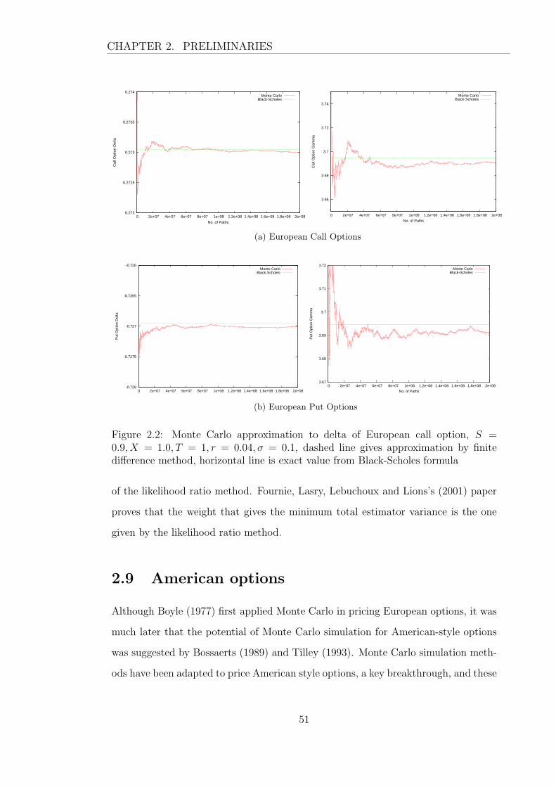
CHAPTER 2. PRELIMINARIES
0.272
0.2725
0.273
0.2735
0.274
0 2e+07 4e+07 6e+07 8e+07 1e+08 1.2e+08 1.4e+08 1.6e+08 1.8e+08 2e+08
Cal
l Opt
ion
Del
ta
No. of Paths
Monte CarloBlack-Scholes
3.66
3.68
3.7
3.72
3.74
0 2e+07 4e+07 6e+07 8e+07 1e+08 1.2e+08 1.4e+08 1.6e+08 1.8e+08 2e+08
Cal
l Opt
ion
Gam
ma
No. of Paths
Monte CarloBlack-Scholes
(a) European Call Options
-0.728
-0.7275
-0.727
-0.7265
-0.726
0 2e+07 4e+07 6e+07 8e+07 1e+08 1.2e+08 1.4e+08 1.6e+08 1.8e+08 2e+08
Put
Opt
ion
Del
ta
Monte CarloBlack-Scholes
3.67
3.68
3.69
3.7
3.71
3.72
0 2e+07 4e+07 6e+07 8e+07 1e+08 1.2e+08 1.4e+08 1.6e+08 1.8e+08 2e+08
Put
Opt
ion
Gam
ma
No. of Paths
Monte CarloBlack-Scholes
(b) European Put Options
Figure 2.2: Monte Carlo approximation to delta of European call option, S =0.9, X = 1.0, T = 1, r = 0.04, σ = 0.1, dashed line gives approximation by finitedifference method, horizontal line is exact value from Black-Scholes formula
of the likelihood ratio method. Fournie, Lasry, Lebuchoux and Lions’s (2001) paper
proves that the weight that gives the minimum total estimator variance is the one
given by the likelihood ratio method.
2.9 American options
Although Boyle (1977) first applied Monte Carlo in pricing European options, it was
much later that the potential of Monte Carlo simulation for American-style options
was suggested by Bossaerts (1989) and Tilley (1993). Monte Carlo simulation meth-
ods have been adapted to price American style options, a key breakthrough, and these
51

CHAPTER 2. PRELIMINARIES
have been developed to be especially suitable for pricing path dependent options and
in tackling high-dimensional problems.
2.9.1 Duality simulation
One technique introduced by Rogers (2002) is called a duality simulation approach
based on a dual characterization of the optimal exercise problem. Rogers illustrates
how to pick a suitable martingale M and take the pathwise maximum of the payoff
less the martingale as the upper bound for the option price. The approach requires a
suitable choice of Lagrangian martingale to give a good result. In his paper, through
using the technique on four specific American style options, with even very simple
choices of M , such as for corresponding European options, the accuracy achieved is
surprising. The same dual simulation approach can be found in the working paper of
Haugh and Kogan (2004), who provide a general algorithm for constructing upper and
lower bounds on the true option price and show the bounds are tight. This means
if the initial approximation is close to the true option value, the bounds are also
guaranteed to be close. In this area, another important contribution is by Broadie
and Glasserman (1997; 2004), who develop two stochastic mesh methods to generate
errors bounds (in the form of confidence intervals) which converge to the correct
price of Bermudan option which is a finitely exercisable American option. Their
algorithm leads to exponential dependence of the computation time on the number
of exercise opportunities rather than the number of assets. The method in Broadie
and Glasserman (2004) requires the computation time to be linear in the number
of exercise opportunities and quadratic in the number of simulation paths. In the
spirit of the papers of Haugh and Kogan (2004) and Rogers (2002), a primal-dual
simulation algorithm is proposed by Andersen and Broadie (2004) to handle any
type of process dynamics, factor structure, and payout specification. Their algorithm
uses an approximation to exercise policy, rather than an approximation to the option
price, to estimate the bounds on the true price of the option. An advantage of
working with the exercise policy is the situation where exercise strategies are known
52

CHAPTER 2. PRELIMINARIES
and independent of option price. These authors also take the martingale part of
supermartingale used in the original approach in Haugh and Kogan (2004) to gain
more accurate estimates.
2.9.2 Regression simulation
Another popular method from a practitioner’s view is based on the regression tech-
nique proposed in Carriere (1996), Tsitsiklis and Van Roy (2001) and Longstaff and
Schwartz (2001). The regression approach is reasonably fast and widely applicable.
Carriere (1996) presents a backward induction algorithm and applies it to calculate
the early exercise premium. He shows that the estimation of the decision rule to
exercise early is equivalent to the estimation of a series of conditional expectations.
The conditional expectations are estimated by splines and local regressions. Tsitsiklis
and Van Roy (2001) proposed a recursive algorithm that approximates the holding
value functions by a linear weighted combination of basis functions directly. Longstaff
and Schwartz (2001) present a simple and powerful approximation to the American
option valuation problem. The main difference to Tsitsiklis and Van Roy (2001)
is the use of least squares to approximate the conditional expectation payoff. The
holder of an American option optimally compares the payoff from immediate exercise
with the expected payoff from continuation. If the immediate payoff is higher, the
holder will choose to exercise the option, otherwise, he will keep the option and wait
for the next exercise opportunity. These authors apply least-squares regression to
find a linear combination of basis functions of the current value of the underlying
to estimate the next time step value. When using regression, the holder takes the
underlying prices as x values and the discounting values of the future underlying price
as y values. As the regression is only dependent on the paths for which the option is
in the money, which significantly increases the efficiency of the algorithm and reduces
computation times. Longstaff and Schwartz (2001) also extend the methodology to
complex derivatives with many underlying factors and, in summary, the accuracy of
the methodology depends on the choice of regression functions. In their empirical
53

CHAPTER 2. PRELIMINARIES
analysis, the authors apply their method to price a wide class of derivatives instru-
ments and show that it yields the best combination of price accuracy and efficiency
against several methodologies employed. In detail, the convergence of least squares
Monte Carlo is described in Cerrato and Cheung (2007), Clement, Lamberton and
Protter (2002) and Rogers (2002). These papers show that the estimated conditional
expectation approaches (with probability one) the true conditional expectation as the
number of basis functions increases, and the number of basis functions determines
the convergence rate of the algorithm. They also prove that the normalized estima-
tion error is asymptotically Gaussian. For a standard put option, Moreno and Navas
(2003) analyze the robustness of the least squares Monte Carlo method relative to the
choice of the type and the number of basis functions. They find the algorithm is very
robust when pricing the American put option and a reasonable approximate value
can be obtained by a modest polynomial degree (between 3 and 20); actually, more
terms can make least square regressions less accurate. Although the Longstaff and
Schwartz method has proved successful and popular, it still suffers from the draw-
back of Monte Carlo convergence. Therefore, Duck, Newton, Widdicks and Leung
(2005) enhance the performance of the least squares Monte Carlo through a conve-
nient and useful procedure. They suggest a formula to describe the variance of the
calculated option from the exact price. The extrapolation procedure entails three
different numbers of paths. After evaluating the averaging put option, they use the
proposed formula to improve the price. The averaging scheme with an extrapolation
procedure does appear to converge better than an order of magnitude faster than the
original scheme of Longstaff and Schwartz. Besides the least squares Monte Carlo
estimator, there is another estimator proposed by Glasserman and Yu (2004), which
is called the weighted Monte Carlo estimator. Broadly speaking, these two methods
are similar, since both aim to evaluate the conditional expectations by a number of
basis functions for regression and finally use Monte Carlo to extract the option price.
There are many other simulation-based methods proposed and, as with the re-
gression approach, they can be used to evaluate the lower bounds on the Bermudan
option value. Andersen (2000) illustrates a method that parameterizes the exercise
54

CHAPTER 2. PRELIMINARIES
policy and then optimizes these parameters over a set of simulations to determine
an approximation to the optimal exercise strategy. Jensen and Svenstrup (2005)
propose a simplification of this exercise strategy, replacing a maximum value of all
(still unexercised) core European options with a carefully chosen single option value.
The numerical test in Jensen and Svenstrup (2005) shows that this simple strategy
leads to a significant computational saving without losses of present values of the
options. Another simulation technique based on parameterizing the exercise decision
is addressed in Garcia (2003). This method uses a parametric representation of the
early exercise decision. This can be constructed by using two different estimates,
one of which is biased low, the other biased high; the two estimates are shown to
be asymptotically unbiased. Very simple representations of the exercise policy can
produce highly accurate option prices. The quantization method proposed in Bally,
Pages and Printems (2002; 2005) is another competitive technique to treat higher-
dimensional problems. Simulation methods based on dimensionality reduction or
nonparametric representations of the early exercise region include Barraquand and
Martineau (1995), Carr and Yang (2001), Clewlow and Strickland (1998), and Ray-
mar and Zwecher (1997). Other papers by Tilley (1993), Barraquand and Martineau
(1995), and Raymar and Zwecher (1997) incorporate different aspects of the usual
backwards induction algorithm by stratifying the state space and finding the optimal
exercise decision in each of the subsets of the state variables.
The Monte Carlo method for derivative securities has reached a fair degree of
maturity. Nevertheless, challenges remain on several fronts. It is certain to be a
continuing goal to develop a better asset price model that is a good fit to data
observed in financial markets. Ever-improving computing technology will expand the
amount and types of data that can be analyzed.
55
Chapter 3
Option Pricing with Jump
Processes
... there is evidence of non-stationarity in the variance. More work
must be done to predict variances using the information available.
– Fischer Black and Myron Scholes
The valuation of option contracts and a test of market efficiency, 1972
In this chapter, we investigate a jump diffusion model which relaxes some of the
restrictive Black-Scholes-Merton model assumptions. Empirical studies have found
that the Black-Scholes model based on Geometric Brownian Motion (GBM) suffers
several defects. One is the asymmetric leptokurtic feature; that is, the return distri-
bution obtained from market data has a higher peak and two (asymmetric) heavier
tails than those of the normal distribution. The constant volatility assumed in the
Black-Scholes model also contradicts an empirical phenomenon, namely the ‘volatil-
ity smile’ in options markets. Another defect is the continuity property of GBM
which fails when markets crash or some large random fluctuations occur. Exten-
sions proposed to model these phenomena can be classified into two groups: jumps
and stochastic-volatility. The stochastic-volatility model was introduced by Hull and
White (1987), then developed by Stein and Stein (1991) and Heston (1993). Also,
stochastic volatility and stochastic interest rate models are presented by Amin and
56

CHAPTER 3. OPTION PRICING WITH JUMP PROCESSES
Ng (1993) and Scott (2002). These models focus on adding more state variables, re-
placing some of the constant parameters used in the Black-Scholes model. The jump
diffusion model is first suggested by Merton (1976), while Cox and Ross (1976) also
provide a pure jump process instead of GBM. Statistical evidence in Ball and Torous
(1985) and Huang and Tauchen (2005) suggest that jumps are significant in financial
markets. Jarrow and Rosenfeld (1984) find the connection between jump risks and
the Capital Asset Pricing Model (CAPM) and Jorion (1988) investigates the existence
of jumps in foreign exchange and stock markets. Andersen and Andreasen (2000) use
the jump-diffusion model to obtain excellent fits with stable parameter estimations
for S&P500 market data. In recent years, some studies indicate the stochastic volatil-
ity model plus jumps leads to improved results. This is because stochastic-volatility
is needed to determine the long-term trend of the volatility process, whilst jumps are
able to model a series of instant changes in the underlying prices that are relatively
large. Bakshi, Cao and Chen (1997) suggest an ideal framework is to include both
jumps and stochastic volatility, which is also supported by Bates (1996). Eraker, Jo-
hannes and Polson (2003) recommend a model with jumps both in the underlying and
the volatility. Andersen, Bollerslev, Diebold and Labys (2001) demonstrate a portion
of realized jumps is caused by stochastic volatility. In his pioneering model, Merton
(1976) proposes jumps according to a compound Poisson process with constant inten-
sity and log-normally distributed jump sizes. Kou’s (2002) work is similar to Merton’s
(1976) model, but with log-double-exponentially distributed jump amplitudes instead
of log-normally distribution. Yan and Hanson (2006) and Zhu and Hanson (2005)
treat the amplitudes as a log-uniformly distribution. Instead of a single class of jumps
used in Merton (1976), Martzoukos (2003) derives a jump-diffusion model with mul-
tiple classes of jumps to describe different types of rare events and makes use of a
joint probability distribution for each class of jumps. For European options, Merton
(1976) derives an analytical expression but, for more exotic options or American op-
tions, no analytical solution exists under jump-diffusion models. Pricing derivatives
on the jump diffusion models can also be related to solve the corresponding partial
integro differential equation (PIDE). Duffy (2008) shows the relationship and propose
57

CHAPTER 3. OPTION PRICING WITH JUMP PROCESSES
several numerical methods.
3.1 Background to the Merton jump diffusion (MJD)
model
We start with the simple Merton (1976) jump diffusion model, written as:
dS = (r − λκ)Sdt+ σSdWS + SdJ , (3.1)
where (r − λκ)dt + σdWS is a Brownian motion with a drift term (r − λκ) rather
than r in the standard Black-Scholes model; λ represents the expected intensity of
jumps during dt and κ is the expected magnitude of the jump size; the additional
term dJ is a compound Poisson jump process to capture the rare events. There is no
dependence between the diffusion term dWS and the jump term dJ . Assuming the
jump size is lognormally distributed, then an explicit analytical solution of European
options with jumps derived in Merton (1976) can be written as:
F (S, τ) =∞∑
n=0
e−λ′τ (λ′τ)n
n!BSn(S, τ ;K, r′, σ′, τ) , (3.2)
where λ′ = λ(1+κ), r′ = r−λκ+n∗ log(1+κ)/τ , σ′ =√σ2 + δ2n/τ , κ = eµ+ 1
2δ2−1
and BSn is the standard Black-Scholes formula of European options with the modi-
fied interest rate r′ and volatility σ′. Here, two new parameters, µ, δ, represent the
intensity of the jump process, namely the mean and standard deviation of the log
jump size, respectively.
It is necessary to point out that the volatility of the Merton model is different from
the Black-Scholes model. In the Black-Scholes case, the t-period standard deviation
of log-return xt is σBS
√t, however in the Merton model, the standard deviation is
√(σ2
Merton + λµ2 + λδ2)t. Normally, we will find an option price from the Merton
model is higher than (or equal to) that from the Black-Scholes model because of the
volatilities of both models, i.e. a larger volatility leads to higher option price:
σBS
√t ≤
√(σ2
Merton + λµ2 + λδ2)t . (3.3)
58

CHAPTER 3. OPTION PRICING WITH JUMP PROCESSES
0
5
10
15
20
25
30 35 40 45 50 55 60 65 70
Eur
opea
n C
all O
ptio
n
Strike K
BSMerton
(a) λ = 1, µ = −0.1, δ = 0.1
0
5
10
15
20
25
30 35 40 45 50 55 60 65 70
Eur
opea
n C
all O
ptio
n
Strike K
BSMerton
(b) λ = 5, µ = −0.1, δ = 0.1
0
5
10
15
20
25
30 35 40 45 50 55 60 65 70
Eur
opea
n C
all O
ptio
n
Strike K
BSMerton
(c) λ = 1, µ = −0.5, δ = 0.1
0
5
10
15
20
25
30 35 40 45 50 55 60 65 70
Eur
opea
n C
all O
ptio
n
Strike K
BSMerton
(d) λ = 1, µ = −0.1, δ = 0.5
Figure 3.1: Pricing European call options by Merton and Black-Scholes models underdifferent parameter sets (shown on the top of each graph). The other parametersapplied here are S = 50, r = 0.05, σ = 0.2 and T = 0.25.
Fig 3.1 provides the Merton option prices calculated by Eq (3.2) and also the corre-
sponding standard Black-Scholes prices. Fig 3.1(a) and Fig 3.1(b) illustrate how the
changes of λ impact on the Merton price accompanied by the Black-Scholes price.
The Merton price generally increases in λ except for deep in or out-of-the-money
(DITM/DOTM) options. The price difference between the two models is more pro-
nounced for at-the-money (ATM) options. Similarly, we also provide the price impact
from mean µ and standard deviation δ of the jump size in Fig 3.1(c) and Fig 3.1(d)
compared with Fig 3.1(a). Reducing µ from −0.1 to −0.5 has more influence on the
option price than the changes of λ as the price increases even for DITM options.
Furthermore, increasing δ gives a higher price of DOTM options. In addition, if we
59
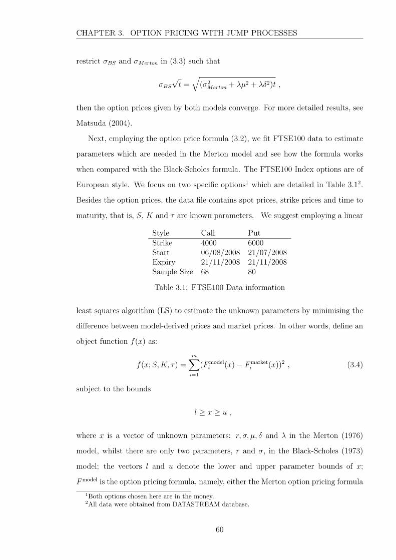
CHAPTER 3. OPTION PRICING WITH JUMP PROCESSES
restrict σBS and σMerton in (3.3) such that
σBS
√t =
√(σ2
Merton + λµ2 + λδ2)t ,
then the option prices given by both models converge. For more detailed results, see
Matsuda (2004).
Next, employing the option price formula (3.2), we fit FTSE100 data to estimate
parameters which are needed in the Merton model and see how the formula works
when compared with the Black-Scholes formula. The FTSE100 Index options are of
European style. We focus on two specific options1 which are detailed in Table 3.12.
Besides the option prices, the data file contains spot prices, strike prices and time to
maturity, that is, S, K and τ are known parameters. We suggest employing a linear
Style Call PutStrike 4000 6000Start 06/08/2008 21/07/2008Expiry 21/11/2008 21/11/2008Sample Size 68 80
Table 3.1: FTSE100 Data information
least squares algorithm (LS) to estimate the unknown parameters by minimising the
difference between model-derived prices and market prices. In other words, define an
object function f(x) as:
f(x;S,K, τ) =m∑
i=1
(Fmodeli (x)− Fmarket
i (x))2 , (3.4)
subject to the bounds
l ≥ x ≥ u ,
where x is a vector of unknown parameters: r, σ, µ, δ and λ in the Merton (1976)
model, whilst there are only two parameters, r and σ, in the Black-Scholes (1973)
model; the vectors l and u denote the lower and upper parameter bounds of x;
Fmodel is the option pricing formula, namely, either the Merton option pricing formula
1Both options chosen here are in the money.2All data were obtained from DATASTREAM database.
60

CHAPTER 3. OPTION PRICING WITH JUMP PROCESSES
(3.2) or the Black-Scholes formula (1973); Fmarket is the corresponding option price
observed in the market, in this example, that is, the FTSE100 Index option price;
m is the sample size given in Table 3.1. The problem of constrained minimization of
f(x) can be solved by the Nag library function (nag opt bounds no deriv). Assuming
the bounds are set as follows:
0.0 ≤ r ≤ 1.0 ,
0.0 ≤ σ ≤ 1.0 ,
−0.2 ≤ µ ≤ 0.0 ,
0.0 ≤ δ ≤ 1.0 ,
0.0 ≤ λ ≤ 5.0 ,
the resulting approximations of the parameters for the both models are presented in
Table 3.2 and the option prices calculated by the option pricing formulae with the
estimated parameters are shown in Fig 3.2.
Model Merton Black-ScholesStyle Call4000 Put6000 Call4000 Put6000
r 0.0000e+00 0.0000e+00 7.1961e-02 7.2847e-02σ 3.3317e-01 0.0000e+00 1.6439e-01 1.6499e-01µ -7.1758e-01 -9.6016e-01 n/a n/aδ 6.0095e-01 2.8495e-01 n/a n/aλ 0.0000e+00 1.2668e-01 n/a n/a
RMSE 67.3452 16.7612 50.5967 19.2470
Table 3.2: Parameter estimators
As shown in Table 3.2, the two sets of data suggest different values of the Merton-
model-implied parameters. The call option data produce a non-jump pure diffusion
model with r = 0 and λ = 0, whilst the put option data results a pure jump diffusion
model with r = 0 and σ = 0. These inconsistent estimates might be explained by
the short term sample period studied here. The entire sample period is just around
two months during the global economic crisis of 2008, which might results in a zero
interest rate. Compared with the Merton model, we observe that the estimates of the
Black-Scholes model: r and σ are approximately equal from both sets of data. The
RMSE value of the Black-Scholes model is less than that of the Merton model for
61

CHAPTER 3. OPTION PRICING WITH JUMP PROCESSES
0
200
400
600
800
1000
1200
1400
1600
1800
0 0.05 0.1 0.15 0.2 0.25 0.3 0.35
Eur
opea
n op
tion
pric
e
time to maturity
European call with K=4000
OptionmarketOptionMERTON
OptionBS
200
400
600
800
1000
1200
1400
1600
1800
2000
2200
0 0.05 0.1 0.15 0.2 0.25 0.3 0.35 0.4
Eur
opea
n op
tion
pric
e
time to maturity
European put with K=6000
OptionmarketOptionMERTON
OptionBS
Figure 3.2: European Option Price from Merton Model against FTSE100 Index Op-tion Price
pricing call options. More precisely, Fig 3.2 shows the Merton model underperforms
the Black-Scholes model for pricing call options close to maturity. These results do
not strongly support the proposition that the Merton model gives a better fit with
FTSE100 Index options against the Black-Scholes model. The main explanations of
the inferior performance of the Merton model are due to adequate sample size and
the simple version of the Merton model used here. It might be improved by involving
the stochastic volatility and market illiquidity which will be introduced in Chapter 4.
3.2 Generating sample paths in the MJD model
The option price formula (3.2) is only available for pricing vanilla European options.
For other complex options on the Merton jump diffusion process (3.1), we are obliged
to employ numerical methods, such as Monte Carlo simulation, to calculate the option
prices. In this section, we give a brief introduction to a numerical method to generate
sample paths under the simple Merton jump diffusion (3.1). Following Glasserman
(2003), the solution of the SDE (3.1) is given by:
S(t) = S(0)e(r−λκ− 12σ2)t+σWS(t)
N(t)∏j=1
Yj , (3.5)
where WS(t) is a standard Brownian motion; N(t) is a Poisson process counting
the number of jumps over [0, t]; Y1, Y2, . . . are random numbers of the jump sizes
from a lognormal distribution LN(µ, δ2); we assume that WS(t), N(t) and Yj are
62
CHAPTER 3. OPTION PRICING WITH JUMP PROCESSES
independent processes. Then the discrete time solution can be obtained at each time
step ti where i = 0, 1, · · · :
S(ti+1) = S(ti)e(r−λκ− 1
2σ2)(ti+1−ti)+σ[WS(ti+1)−WS(ti)]
N(ti+1)∏
j=N(ti)+1
Yj . (3.6)
A simplification of the solution (3.6) can be found by taking logarithms of both sides
of (3.6) and replacing log S(ti) with x(ti), which is
x(ti+1) = x(ti)+(r−λκ−1
2σ2)(ti+1−ti)+σ[WS(ti+1)−WS(ti)]+
N(ti+1)∑
j=N(ti)+1
log Yj . (3.7)
This representation is preferable, because it uses the sums of log Yj instead of the
products of Yj, and log Yj can be directly simulated from a normal distribution
N(µ, δ2). The option price S(ti) is estimated by exponentiating x(ti), which is easily
implemented.
To generate sample paths x(ti) following Eq (3.7), the diffusion term [WS(ti+1)−WS(ti)] can be simulated by the product of a standard normal random variable Zi
from N(0, 1) and the square root of the time difference√ti+1 − ti. For the jump
term, the number of jumps over [ti, ti+1] also has a Poisson distribution with mean
λ(ti+1−ti), therefore instead of simulating the jumps individually, we can estimate the
total effect of the jumps over [ti, ti+1] by a normal random variable from N(µξi, δ2ξi)
with ξi is the realized possible random variable, that is,
N(ti+1)∑
j=N(ti)+1
log Yj ∼ N(µξi, δ2ξi) = µξi + δ
√ξiN(0, 1) .
The algorithm for simulation is given by the following steps:
1. generate Zi ∼ N(0, 1)
2. generate ξi ∼ Poisson(λ(ti+1 − ti)); if ξi = 0, set ηi = 0 and go to Step 4
3. generate Zi ∼ Normal(0, 1); set ηi = µξi + δ√ξiZi
4. set
x(ti+1) = x(ti) + (r − λκ− 1
2σ2)(ti+1 − ti) + σ
√ti+1 − tiZi + ηi (3.8)
63

CHAPTER 3. OPTION PRICING WITH JUMP PROCESSES
5. transfer to underlying price S
S(ti) = exp(x(ti)) .
Then, the standard Monte Carlo method is used with a number of sample paths
generated by the above algorithm to compute the option price. An example is given
in Fig 3.3. The straight line in each case is produced by Merton’s analytical solution
12.4
12.5
12.6
12.7
12.8
12.9
13
0 1e+06 2e+06 3e+06 4e+06 5e+06 6e+06 7e+06 8e+06 9e+06 1e+07
Eur
opea
n ca
ll op
tion
pric
e
no. of runs
Monte Carlo methodMerton method (12.7166)
7.74
7.76
7.78
7.8
7.82
7.84
7.86
7.88
7.9
7.92
7.94
0 2e+006 4e+006 6e+006 8e+006 1e+007 1.2e+007 1.4e+007 1.6e+007 1.8e+007 2e+007
Eur
opea
n pu
t opt
ion
pric
e
no. of paths
Monte Carlo methodMerton method (7.83955)
Figure 3.3: Pricing European options by Merton and Monte Carlo methods, S =K = 100, r = 0.05, σ = 0.2, T = 1, λ = 0.1, δ = 0.8, µ = −δ2/2.
(3.2) as a benchmark. Fig 3.3 shows that the Monte Carlo estimation converges to
the Merton value with an increasing number of sample paths, which suggests the
above algorithm is valid for estimating option prices.
3.3 Pricing 1D Bermudan put options using the
MJD model
This section introduces the pricing of a Bermudan put option via Monte Carlo meth-
ods in a jump diffusion model. A Bermudan option allows the holder to exercise at a
fixed number of dates, in contrast with an American option, which can be exercised
at any time. As mentioned in Section 2.9, in recent years, the Monte Carlo method
has been extended to handle early exercise for American and Bermudan options. We
extend the Longstaff and Schwartz (2001), Least Squares Monte Carlo method (LSM)
to corporate the jump diffusion model, in particular the method of Duck et al. (2005)
is employed to enhance accuracy.
64
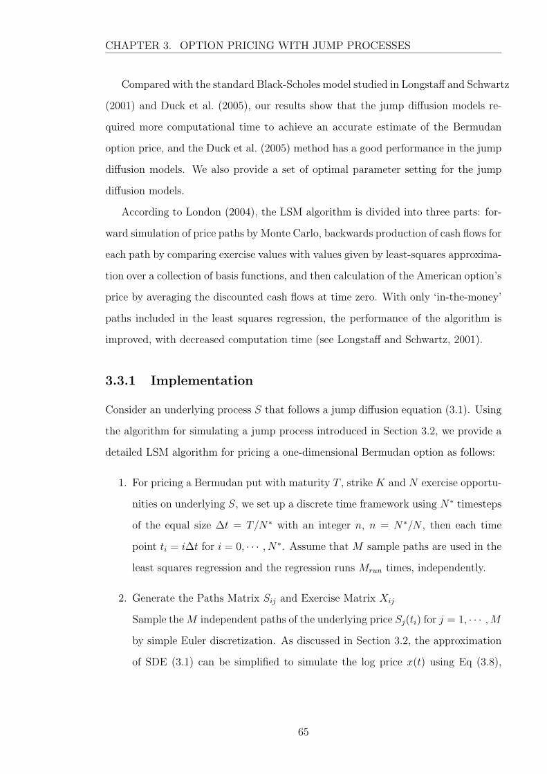
CHAPTER 3. OPTION PRICING WITH JUMP PROCESSES
Compared with the standard Black-Scholes model studied in Longstaff and Schwartz
(2001) and Duck et al. (2005), our results show that the jump diffusion models re-
quired more computational time to achieve an accurate estimate of the Bermudan
option price, and the Duck et al. (2005) method has a good performance in the jump
diffusion models. We also provide a set of optimal parameter setting for the jump
diffusion models.
According to London (2004), the LSM algorithm is divided into three parts: for-
ward simulation of price paths by Monte Carlo, backwards production of cash flows for
each path by comparing exercise values with values given by least-squares approxima-
tion over a collection of basis functions, and then calculation of the American option’s
price by averaging the discounted cash flows at time zero. With only ‘in-the-money’
paths included in the least squares regression, the performance of the algorithm is
improved, with decreased computation time (see Longstaff and Schwartz, 2001).
3.3.1 Implementation
Consider an underlying process S that follows a jump diffusion equation (3.1). Using
the algorithm for simulating a jump process introduced in Section 3.2, we provide a
detailed LSM algorithm for pricing a one-dimensional Bermudan option as follows:
1. For pricing a Bermudan put with maturity T , strike K and N exercise opportu-
nities on underlying S, we set up a discrete time framework using N∗ timesteps
of the equal size ∆t = T/N∗ with an integer n, n = N∗/N , then each time
point ti = i∆t for i = 0, · · · , N∗. Assume that M sample paths are used in the
least squares regression and the regression runs Mrun times, independently.
2. Generate the Paths Matrix Sij and Exercise Matrix Xij
Sample theM independent paths of the underlying price Sj(ti) for j = 1, · · · ,Mby simple Euler discretization. As discussed in Section 3.2, the approximation
of SDE (3.1) can be simplified to simulate the log price x(t) using Eq (3.8),
65
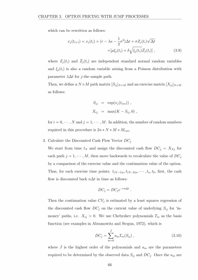
CHAPTER 3. OPTION PRICING WITH JUMP PROCESSES
which can be rewritten as follows:
xj(ti+1) = xj(ti) + (r − λκ− 1
2σ2)∆t+ σZj(ti)
√∆t
+[µξj(ti) + δ√ξj(ti)Zj(ti)] , (3.9)
where Zj(ti) and Zj(ti) are independent standard normal random variables
and ξj(ti) is also a random variable arising from a Poisson distribution with
parameter λ∆t for j-the sample path.
Then, we define a N×M path matrix [Sij]N×M and an exercise matrix [Xij]N×M
as follows:
Sij = exp(xj(ti∗n)) ,
Xij = max(K − Sij, 0) ,
for i = 0, · · · , N and j = 1, · · · ,M . In addition, the number of random numbers
required in this procedure is 2n ∗N ∗M ∗Mrun.
3. Calculate the Discounted Cash Flow Vector DCj
We start from time tN and assign the discounted cash flow DCj = XNj for
each path j = 1, · · · ,M , then move backwards to recalculate the value of DCj
by a comparison of the exercise value and the continuation value of the option.
Thus, for each exercise time points: t(N−1)n, t(N−2)n, · · · , tn, t0, first, the cash
flow is discounted back n∆t in time as follows:
DCj = DCje−rn∆t .
Then the continuation value CVj is estimated by a least squares regression of
the discounted cash flow DCj on the current value of underlying Sij for ‘in-
money’ paths, i.e. Xij > 0. We use Chebyshev polynomials Tm as the basis
function (see examples in Abramowitz and Stegun, 1972), which is
DCj =J∑
m=0
amTm(Sij) , (3.10)
where J is the highest order of the polynomials and am are the parameters
required to be determined by the observed data Sij and DCj. Once the am are
66

CHAPTER 3. OPTION PRICING WITH JUMP PROCESSES
known, we can approximate the continuation value as follows:
CVj =J∑
m=0
amTm(Sij) . (3.11)
If Xij > CVj, we exercise the put option and replace the value DCj = Xij;
otherwise, we hold the option and keep the value of DCj. We repeat this
procedure until t0.
4. Average the discounted cash flows over the M sample paths, that is,
P =1
M
M∑j=1
DCj .
5. Repeat Step 2 to Step 4 for Mrun times and take the average value of P as
the estimator of the Bermudan put price. There is an alternative procedure
proposed in Duck et al. (2005) which is shown to achieve a more accurate
estimated price. Their method, based on an extrapolation technique, can be
easily implemented with three different sample sizes M . We will give a detailed
description of the method and numerical examples in Section 3.5.4.
3.3.2 Sensitivity of option price to the choice of the param-
eters
In this section, we study the sensitivity of the input parameters used in the algorithm
in Section 3.3.1 to the option price, which are the sample size M for the least squares
regression, the expected number of jumps λ and the size of time steps ∆t discussed
respectively in the following:
1. Sample Size M Impact on Option Price
First, the choice of the sample size plays a critical role in the Least Squares
Monte Carlo algorithm. In a case without jumps, as we increase exercise oppor-
tunities, the price of a Bermudan put option rises and tends to be an asymptotic
value in the limit, which is the case of pricing an American option. This rule
should hold in the case with jumps, so it can be used to test whether the choice
67
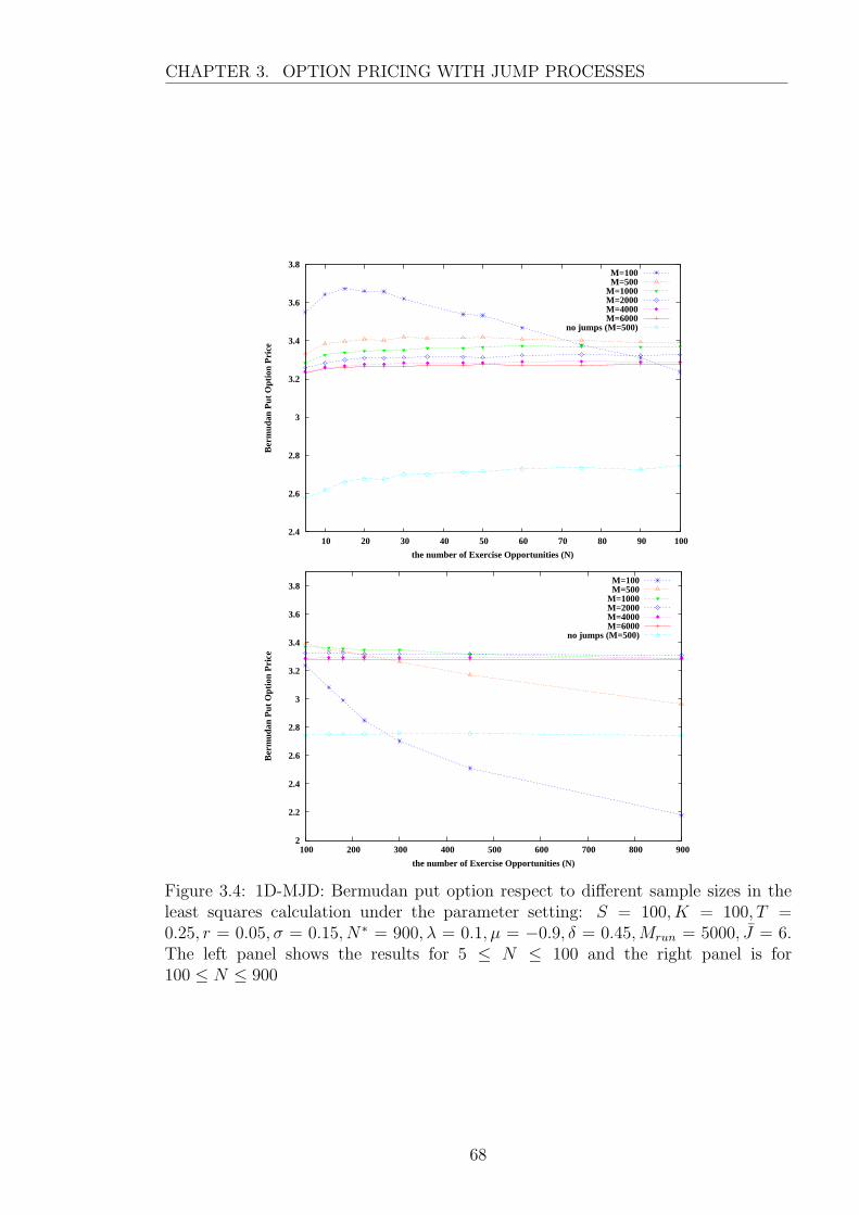
CHAPTER 3. OPTION PRICING WITH JUMP PROCESSES
2.4
2.6
2.8
3
3.2
3.4
3.6
3.8
10 20 30 40 50 60 70 80 90 100
Ber
mud
an P
ut O
ptio
n P
rice
the number of Exercise Opportunities (N)
M=100M=500
M=1000M=2000M=4000M=6000
no jumps (M=500)
2
2.2
2.4
2.6
2.8
3
3.2
3.4
3.6
3.8
100 200 300 400 500 600 700 800 900
Ber
mud
an P
ut O
ptio
n P
rice
the number of Exercise Opportunities (N)
M=100M=500
M=1000M=2000M=4000M=6000
no jumps (M=500)
Figure 3.4: 1D-MJD: Bermudan put option respect to different sample sizes in theleast squares calculation under the parameter setting: S = 100, K = 100, T =0.25, r = 0.05, σ = 0.15, N∗ = 900, λ = 0.1, µ = −0.9, δ = 0.45,Mrun = 5000, J = 6.The left panel shows the results for 5 ≤ N ≤ 100 and the right panel is for100 ≤ N ≤ 900
68

CHAPTER 3. OPTION PRICING WITH JUMP PROCESSES
of sample sizeM is appropriate to value the option price. GivenM for the least
squares algorithm, Fig 3.4 shows the Bermudan option prices with respect to
the total number of exercise times N ranging from 5 to 900, assuming the total
number of time steps N∗ is taken to be 900 for this example. We also calculate
the prices of the corresponding Bermudan options in the Black-Scholes model
by setting λ = 0 in the same algorithm, i.e. no jumps in the underlyings. Fig 3.4
shows that the choice of sample size M is important to achieve an acceptable
Bermudan option price, because the option prices estimated by fewer sample
paths, such as M = 100 and 500, increase initially then decrease with increasing
N . This decline is spurious and against the expected trend stated above. The
problem can be easily resolved by increasing the sample size, M . As shown
in Fig 3.4, the option price for M = 2000, 4000 and 6000 slightly increases for
relatively small values N , whilst for larger values of N the option price tends
to be fairly constant, that can be recognised as the price of the corresponding
American option price with infinite exercise opportunities. Compared with the
Black-Scholes model where the sample size M = 500 is sufficient to produce a
reasonable price of the Bermudan option, the MJD model requires more sample
paths to yield the Bermudan option price, due to more volatility involved in
the underlying. The results in Fig 3.4 suggest that an adequate sample size is
M = 2000 for the least squares regression in the MJD model. When the sample
size rises from 2000 to 6000, the option price slightly decreases and converges
to an asymptotic value for the Bermudan option with N exercise opportunity.
With a proper value of M , we find that the Bermudan prices in the MJD model
are higher than the prices in the Black-Scholes model without jumps, which
implies that the underlying asset becomes more volatile when including jump
events.
Fig 3.5 shows a comparison of option prices between Mrun = 5000 and Mrun =
10000 for different values of M . In general, the computational time required for
Mrun = 10000 is about twice as much as the time required for Mrun = 5000 (see
69
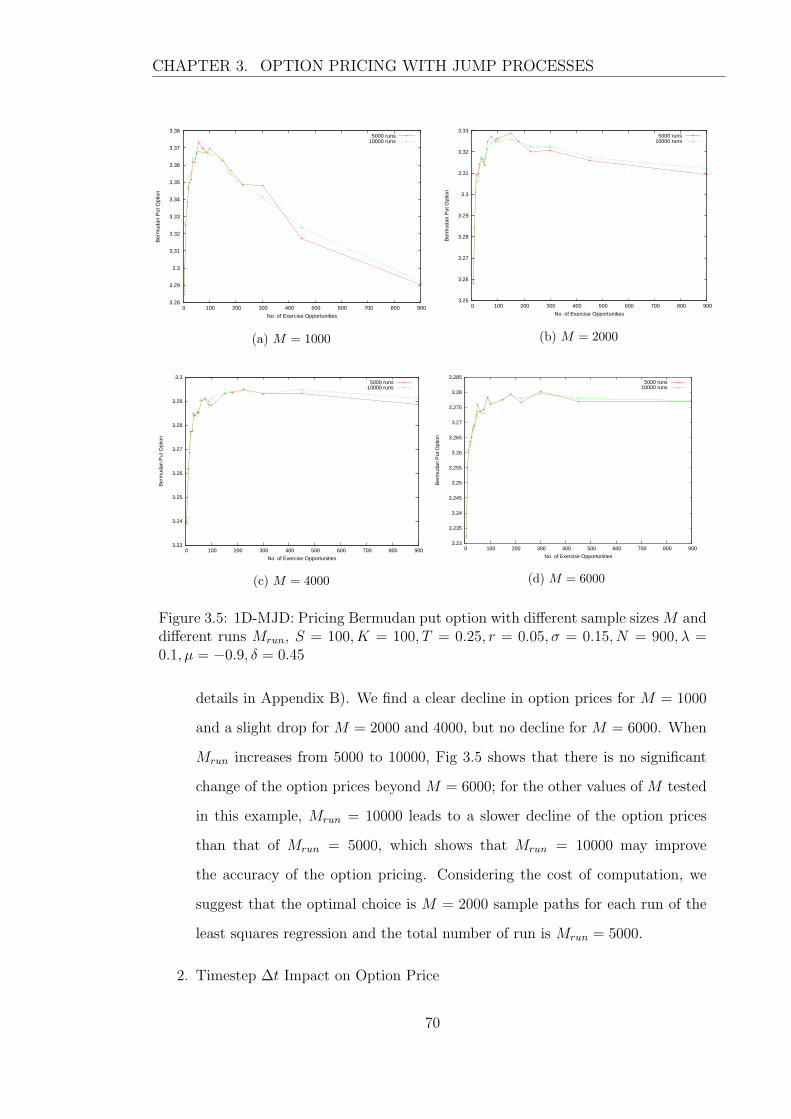
CHAPTER 3. OPTION PRICING WITH JUMP PROCESSES
3.28
3.29
3.3
3.31
3.32
3.33
3.34
3.35
3.36
3.37
3.38
0 100 200 300 400 500 600 700 800 900
Ber
mud
an P
ut O
ptio
n
No. of Exercise Opportunities
5000 runs10000 runs
(a) M = 1000
3.25
3.26
3.27
3.28
3.29
3.3
3.31
3.32
3.33
0 100 200 300 400 500 600 700 800 900
Ber
mud
an P
ut O
ptio
n
No. of Exercise Opportunities
5000 runs10000 runs
(b) M = 2000
3.23
3.24
3.25
3.26
3.27
3.28
3.29
3.3
0 100 200 300 400 500 600 700 800 900
Ber
mud
an P
ut O
ptio
n
No. of Exercise Opportunities
5000 runs10000 runs
(c) M = 4000
3.23
3.235
3.24
3.245
3.25
3.255
3.26
3.265
3.27
3.275
3.28
3.285
0 100 200 300 400 500 600 700 800 900
Ber
mud
an P
ut O
ptio
n
No. of Exercise Opportunities
5000 runs10000 runs
(d) M = 6000
Figure 3.5: 1D-MJD: Pricing Bermudan put option with different sample sizes M anddifferent runs Mrun, S = 100, K = 100, T = 0.25, r = 0.05, σ = 0.15, N = 900, λ =0.1, µ = −0.9, δ = 0.45
details in Appendix B). We find a clear decline in option prices for M = 1000
and a slight drop for M = 2000 and 4000, but no decline for M = 6000. When
Mrun increases from 5000 to 10000, Fig 3.5 shows that there is no significant
change of the option prices beyond M = 6000; for the other values of M tested
in this example, Mrun = 10000 leads to a slower decline of the option prices
than that of Mrun = 5000, which shows that Mrun = 10000 may improve
the accuracy of the option pricing. Considering the cost of computation, we
suggest that the optimal choice is M = 2000 sample paths for each run of the
least squares regression and the total number of run is Mrun = 5000.
2. Timestep ∆t Impact on Option Price
70

CHAPTER 3. OPTION PRICING WITH JUMP PROCESSES
7.05
7.1
7.15
7.2
7.25
7.3
0 500 1000 1500 2000 2500 3000 3500 4000 4500 5000
Ber
mud
an p
ut o
ptio
n pr
ice
No.of runs (Nrun)
∆t=1/12∆t=1/120
∆t=1/2400∆t=1/6000
∆t=1/12000∆t=1/18000
Figure 3.6: 1D-MJD: Pricing Bermudan put option with different sizes of timesteps∆t with the parameter setting: S = 100, K = 100, T = 1.0, r = 0.05, σ = 0.15, λ =0.1, µ = −0.9, δ = 0.45, N = 12 and Mrun = 10000
The timestep ∆t is a factor for consideration in discrete-time approximation
error for general Monte Carlo simulations. The algorithm in Section 3.3.1 sug-
gests simulating underlying prices at each time point ti+1 = ti +∆t to minimize
discretization error by choosing a small value of ∆t. Here, we show that, what-
ever ∆t is applied, the simulated sample paths according to Eq (3.9) lead to
accurate values for a Bermudan options. In Fig 3.6, varying values of ∆t have
been examined to estimate a Bermudan put option with N = 12 exercise op-
portunities. We find that there is no obvious effect of ∆t on the option prices.
Indeed, the price given by ∆t = 1/12, leading to the same time points as early
exercises, is similar to those prices estimated by smaller values of ∆t, because
SDE (3.1) is solved exactly. Therefore, we can directly simulate the underlying
price at each exercise time point, i.e. setting n = 1 in the original algorithm in
Section 3.3.1.
3.3.3 λ impact on pricing option
The parameter λ in a jump process is a rate representing the expected number of
arrivals per unit time. A higher λ implies more jumps during the option’s life, which
71

CHAPTER 3. OPTION PRICING WITH JUMP PROCESSES
implies more volatility associated with the underlying. As discussed in Section 3.1,
using the analytical solution (3.2), we find that the prices of European-style options
increase as λ values rise, just as expected for option prices as volatility is increased.
Table 3.3 shows how the value of a Bermudan option changes with different values of λ
λ European put price Bermudan put price Bermudan put price(N = 12) (N = 30)
0 3.7146 4.2457 4.30041 27.4128 28.8465 28.994710 72.6870 74.4841 74.646320 86.3417 88.4513 88.5845
Table 3.3: 1D-MJD: Impact of λ on pricing Bermudan and European options underthe following parameter setting: S = K = 100, T = 1, r = 0.05, σ = 0.15, µ =−0.9, δ = 0.45,M = 2000 and Mrun = 5000. The results for European options arecalculated by Eq (3.2).
compared with a standard European put option in the same MJD model. Intuitively,
the Bermudan option is more expensive than the European option. When λ rises,
the price of the Bermudan option increases as in the case of the European price.
Moreover, the option prices for λ 6= 0 are much higher than the prices for λ = 0.
This is because, when we set the mean of jump-size µ to be negative, there is a high
probability money can be made from trades with lower asset prices (immediately for
those Bermudan option holders). Table 3.3 also provides two kinds of Bermudan
options with the different number of exercise times: N = 12 and N = 30. We can see
that the option price given by N = 30 is slightly higher than the price for N = 12
in each case of λ, which is consistent with the previous results with regard to N in
Fig 3.4.
3.4 Pricing multi-dimensional Bermudan put op-
tion using the MJD model
In this section, we extend our one-dimensional model in Section 3.3 to pricing a
Bermudan option on multiple underlying assets with jumps. The main difficulty
with pricing those options is to find the correlations of the intensities and sizes of
72
CHAPTER 3. OPTION PRICING WITH JUMP PROCESSES
the jumps among different assets. There are three kinds of approaches: independent
jumps, jumps with the same intensities but different sizes and jumps with different
intensities and sizes. As an example of the first case, Merton (1976) set up a hedged
portfolio with m stocks. He supposed the jump components of a stock’s return were
totally independent in the portfolio. For the second case, Duffie et al. (2000) illustrate
a stochastic volatility model and apply the jumps into both the underlying and the
volatility (referred to as SVJJ). In the SVJJ model, it is assumed that the jumps on
the underlying arrive at the same time as those on the volatility process, that is, two
processes are employed with the same number of jumps at time t, N vt = N s
t = N , and
the correlated jump sizes are ξv ∼ Exp(µv) and ξs|ξv ∼ Normal(µs + ρJ Zv, (δs)2).
Martzoukos (2003) introduces a foreign asset model with multiple classes of jumps.
He assumes that the jumps from the same class can affect several or all asset prices
with a correlation matrix of jump size for different assets, while the jumps from the
different classes are totally independent. The same assumption has been applied by
Clift (2007) in his thesis, who uses finite-difference methods to price options with a
two-asset jump diffusion. Matei (2005) considers two kinds of jumps: idiosyncratic
jumps and common jumps, which happen independently, in a multi-asset model. The
former is determined by the specific asset itself, and leaves the other assets unaffected,
whereas the latter affects all the assets at the same time, except for those specific
assets. For common jumps, it is natural to consider the correlation of the jump sizes
among different assets. The third approach concerning the correlation of the jump
intensities is introduced in Chan’s (2003) paper. He suggests that the number of
jumps for the p-asset is Np = N∗p + N , where N∗
p and N are independent Poisson
random variables with intensities µ∗p and µ. Based on Chan’s (2003) and Clift’s
(2007) models, we consider the correlated intensities and sizes of jumps on assets
Sp for p = 1 · · ·P . If the jumps happen at the same time, there is a correlation
coefficient, ρJ , for jump sizes which follows a multivariate normal distribution. We
also consider a correlation coefficient, ρn, of jumps arrivals. For a multi-asset case,
73

CHAPTER 3. OPTION PRICING WITH JUMP PROCESSES
the model under log-price scale, xp = log Sp, is obtained as follows:
dxp = (r − λpκp − 1
2σ2
p)dt+ σpdWp + Jpdqp , (3.12)
where
κp = exp(µp +1
2δ2p)− 1 ,
ξ∗p ∼ Poisson(λpdt) ,
ξ∗ ∼ Poisson(λdt),
dqp = ξ∗p + ξ∗ ,
(J1, · · · , JP ) ∼ N(µ1, · · · , µP ; δ21, · · · , δ2
P ; ΣJ) ,
which is a multivariate normal distribution of jump size on different assets, with a
correlation matrix ΣJ ; similarly, the increments of Brownian motion dWp are derived
from a multivariate normal distribution with mean zero, which is
(dW1, · · · , dWP ) ∼ Normal(0; dt; ΣW ) ,
with the correlation matrix ΣW , the vector of mean 0 and the vector of variance dt.
3.4.1 Implementation
The Monte Carlo method gains advantage over other numerical methods whose com-
putational cost increases exponentially rather than linearly with an increasing number
of underlyings. LSM is easily implemented and an effective choice in pricing options
on multi-underlying Bermudan-style valuations. Consider a Bermudan put option on
P correlated underlying assets, whose the payoff V is given by:
V = max(0, K1 − S1(tN), · · · , Kp − Sp(tN), · · · , KP − SP (tN)) , (3.13)
where Kp is a strike price according to the p-th underlying asset. Now consider the
Euler discretization of SDE (3.12) over small time intervals ∆t where ti+1 = ti + ∆t,
we gain the approximation as follows:
xp(ti+1) = xp(ti) + (r − λpκp − 1
2(σp)2)∆t+ σpZp(ti)
√∆t+ Jp(ti)∆q
p(ti), (3.14)
74
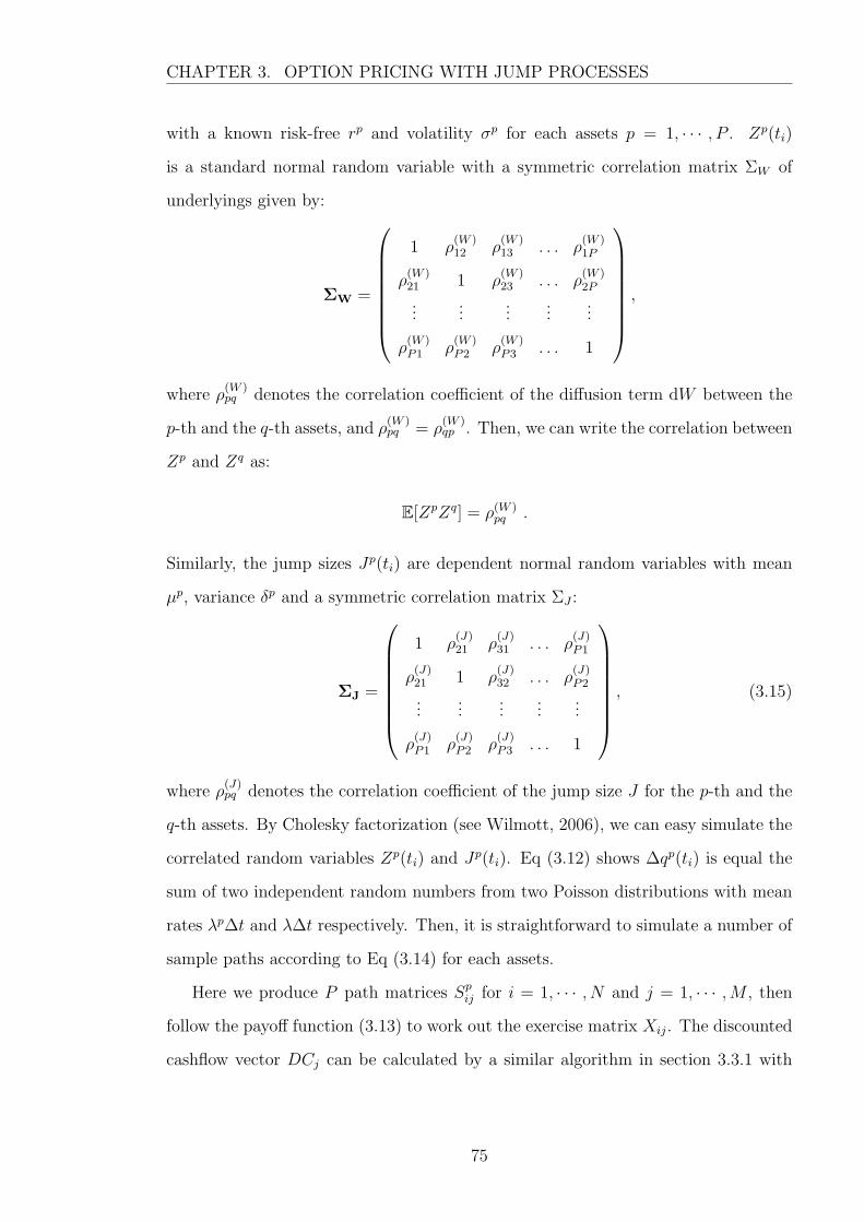
CHAPTER 3. OPTION PRICING WITH JUMP PROCESSES
with a known risk-free rp and volatility σp for each assets p = 1, · · · , P . Zp(ti)
is a standard normal random variable with a symmetric correlation matrix ΣW of
underlyings given by:
ΣW =
1 ρ(W )12 ρ
(W )13 . . . ρ
(W )1P
ρ(W )21 1 ρ
(W )23 . . . ρ
(W )2P
......
......
...
ρ(W )P1 ρ
(W )P2 ρ
(W )P3 . . . 1
,
where ρ(W )pq denotes the correlation coefficient of the diffusion term dW between the
p-th and the q-th assets, and ρ(W )pq = ρ
(W )qp . Then, we can write the correlation between
Zp and Zq as:
E[ZpZq] = ρ(W )pq .
Similarly, the jump sizes Jp(ti) are dependent normal random variables with mean
µp, variance δp and a symmetric correlation matrix ΣJ :
ΣJ =
1 ρ(J)21 ρ
(J)31 . . . ρ
(J)P1
ρ(J)21 1 ρ
(J)32 . . . ρ
(J)P2
......
......
...
ρ(J)P1 ρ
(J)P2 ρ
(J)P3 . . . 1
, (3.15)
where ρ(J)pq denotes the correlation coefficient of the jump size J for the p-th and the
q-th assets. By Cholesky factorization (see Wilmott, 2006), we can easy simulate the
correlated random variables Zp(ti) and Jp(ti). Eq (3.12) shows ∆qp(ti) is equal the
sum of two independent random numbers from two Poisson distributions with mean
rates λp∆t and λ∆t respectively. Then, it is straightforward to simulate a number of
sample paths according to Eq (3.14) for each assets.
Here we produce P path matrices Spij for i = 1, · · · , N and j = 1, · · · ,M , then
follow the payoff function (3.13) to work out the exercise matrix Xij. The discounted
cashflow vector DCj can be calculated by a similar algorithm in section 3.3.1 with
75
CHAPTER 3. OPTION PRICING WITH JUMP PROCESSES
replacing Eq (3.10) and (3.11) with
DCj =
J1∑m1=0
J2∑m2=0
· · ·Jp∑
mp=0
· · ·JP∑
mP =0
(κ(m1,m2, · · · ,mp, · · · ,mP )
×am1,m2,··· ,mp,··· ,mPTm1(S
1ij)Tm2(S
2ij) · · ·Tmp(S
pij) · · ·TmP
(SPij )
), (3.16)
and
CVj =
J1∑m1=0
J2∑m2=0
· · ·Jp∑
mp=0
· · ·JP∑
mP =0
(κ(m1,m2, · · · ,mp, · · · ,mP )
×am1,m2,··· ,mp,··· ,mPTm1(S
1ij)Tm2(S
2ij) · · ·Tmp(S
pij) · · ·TmP
(SPij )
), (3.17)
where Tmp is the m-th Chebyshev polynomial corresponding to the p-th underlying;
Jp is the highest order of the polynomials of the p-th underlying, generally chosen
as J1 = J2 = · · · = JP = J ; the am1,m2,··· ,mPare the coefficients to be least square
approximated; κ is an indicator function, which is
κ(m1,m2, · · · ,mp, · · · ,mP ) =
1 if∑p=P
p=1 (mp) ≤ J ,
0 if∑i=P
p=1 (mp) > J .
We use the trace function to eliminate unnecessary computations and save calculation
time. As mentioned in Duck et al. (2005), the choice of J and M is important to
option pricing. If J is big enough and M is sufficiently large, LSM will produce an
accurate estimate for the price of a Bermudan option.
3.4.2 Numerical results
In this section, we study the impact of the highest order of Chebyshev polynomials J
and sample size M on pricing two dimensional Bermudan options via three examples
with the different numbers of exercise opportunities. The parameters employed in
the examples are shown in Table 3.4. Fig 3.7 provides the results from pricing
Bermudan put options for varying J and M when exercise times N = 2, 10 and 25,
respectively. It is (theoretically) expected that the red plane should be on the top,
having the most exercise times (N = 25), followed by the green surface (N = 10)
and the blue surface (N = 2). However, this cannot hold when those values of J and
76

CHAPTER 3. OPTION PRICING WITH JUMP PROCESSES
Parameter ValueSp(t0) 100Kp 100r 0.05σp 0.15T 1.0
ρ(W )21 0.2
ρ(J)21 0.2λp = λ 0.1µp −0.9δp 0.45n 100∆t 1/(N ∗ n)p 1, 2
Table 3.4: This set of parameters is used to demonstrate the numerical approach ofpricing a Bermudan put under two assets with jump diffusion.
M are relatively small. It is clear that increasing J and M reduces the error of the
estimated option prices, while it also increases the computing budget. From Fig 3.7,
we find that the option price will tend to rise as J increases, whereas the option price
will reduce as M rises. Considering a trade-off between accuracy and computational
cost, we recommend that the optimal choice is J = 12 and M = 70000. For those
proper values of J and M , the difference between the prices given by N = 10 and
N = 25 is slight, while the price for N = 2 is much lower than both of them.
Moreover, the estimated price for N = 10 and N = 25 is more sensitive to the choice
of J and M than the price of N = 2, which suggests that we usually need to choose
larger values of J and M when pricing a Bermudan option with more exercise times.
3.5 Pricing 1D Bermudan put option using the
double-jump stochastic volatility (SVJJ) model
As noted in Section 3.4, Duffie et al. (2000) derive an affine jump-diffusion model.
Based on the variance model studied by Heston (1993), a two-factor jump process
is derived to price options when jumps occur in both the underlying and volatility.
The occurrences of jumps are governed by a Poisson process with intensity λdt; for
77
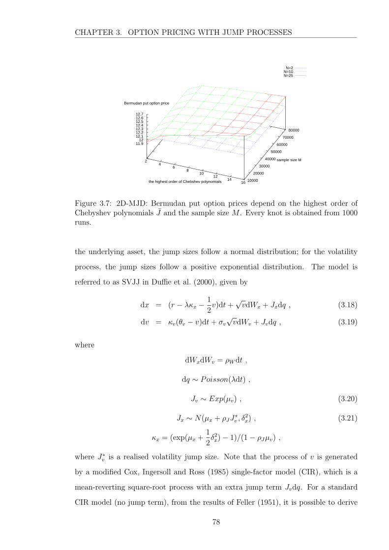
CHAPTER 3. OPTION PRICING WITH JUMP PROCESSES
N=2N=10N=25
2 4
6 8
10 12
14 16the highest order of Chebshev polynomials 10000
20000
30000
40000
50000
60000
70000
80000
sample size M
11.9 12
12.1 12.2 12.3 12.4 12.5 12.6 12.7
Bermudan put option price
Figure 3.7: 2D-MJD: Bermudan put option prices depend on the highest order ofChebyshev polynomials J and the sample size M . Every knot is obtained from 1000runs.
the underlying asset, the jump sizes follow a normal distribution; for the volatility
process, the jump sizes follow a positive exponential distribution. The model is
referred to as SVJJ in Duffie et al. (2000), given by
dx = (r − λκx − 1
2v)dt+
√vdWx + Jxdq , (3.18)
dv = κv(θv − v)dt+ σv
√vdWv + Jvdq , (3.19)
where
dWxdWv = ρW dt ,
dq ∼ Poisson(λdt) ,
Jv ∼ Exp(µv) , (3.20)
Jx ∼ N(µx + ρJJ∗v , δ
2x) , (3.21)
κx = (exp(µx +1
2δ2x)− 1)/(1− ρJµv) ,
where J∗v is a realised volatility jump size. Note that the process of v is generated
by a modified Cox, Ingersoll and Ross (1985) single-factor model (CIR), which is a
mean-reverting square-root process with an extra jump term Jvdq. For a standard
CIR model (no jump term), from the results of Feller (1951), it is possible to derive
78
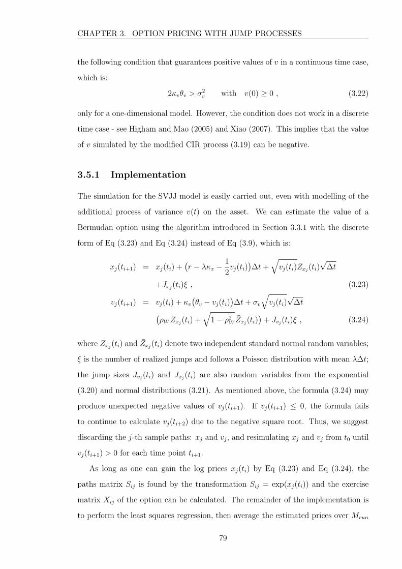
CHAPTER 3. OPTION PRICING WITH JUMP PROCESSES
the following condition that guarantees positive values of v in a continuous time case,
which is:
2κvθv > σ2v with v(0) ≥ 0 , (3.22)
only for a one-dimensional model. However, the condition does not work in a discrete
time case - see Higham and Mao (2005) and Xiao (2007). This implies that the value
of v simulated by the modified CIR process (3.19) can be negative.
3.5.1 Implementation
The simulation for the SVJJ model is easily carried out, even with modelling of the
additional process of variance v(t) on the asset. We can estimate the value of a
Bermudan option using the algorithm introduced in Section 3.3.1 with the discrete
form of Eq (3.23) and Eq (3.24) instead of Eq (3.9), which is:
xj(ti+1) = xj(ti) +(r − λκx − 1
2vj(ti)
)∆t+
√vj(ti)Zxj
(ti)√
∆t
+Jxj(ti)ξ , (3.23)
vj(ti+1) = vj(ti) + κv
(θv − vj(ti)
)∆t+ σv
√vj(ti)
√∆t
(ρWZxj
(ti) +√
1− ρ2W Zxj
(ti))
+ Jvj(ti)ξ , (3.24)
where Zxj(ti) and Zxj
(ti) denote two independent standard normal random variables;
ξ is the number of realized jumps and follows a Poisson distribution with mean λ∆t;
the jump sizes Jvj(ti) and Jxj
(ti) are also random variables from the exponential
(3.20) and normal distributions (3.21). As mentioned above, the formula (3.24) may
produce unexpected negative values of vj(ti+1). If vj(ti+1) ≤ 0, the formula fails
to continue to calculate vj(ti+2) due to the negative square root. Thus, we suggest
discarding the j-th sample paths: xj and vj, and resimulating xj and vj from t0 until
vj(ti+1) > 0 for each time point ti+1.
As long as one can gain the log prices xj(ti) by Eq (3.23) and Eq (3.24), the
paths matrix Sij is found by the transformation Sij = exp(xj(ti)) and the exercise
matrix Xij of the option can be calculated. The remainder of the implementation is
to perform the least squares regression, then average the estimated prices over Mrun
79
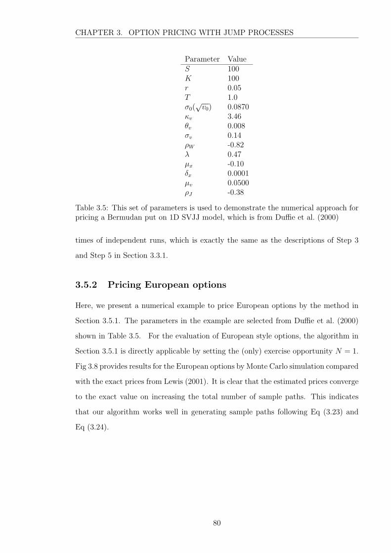
CHAPTER 3. OPTION PRICING WITH JUMP PROCESSES
Parameter ValueS 100K 100r 0.05T 1.0σ0(√v0) 0.0870
κv 3.46θv 0.008σv 0.14ρW -0.82λ 0.47µx -0.10δx 0.0001µv 0.0500ρJ -0.38
Table 3.5: This set of parameters is used to demonstrate the numerical approach forpricing a Bermudan put on 1D SVJJ model, which is from Duffie et al. (2000)
times of independent runs, which is exactly the same as the descriptions of Step 3
and Step 5 in Section 3.3.1.
3.5.2 Pricing European options
Here, we present a numerical example to price European options by the method in
Section 3.5.1. The parameters in the example are selected from Duffie et al. (2000)
shown in Table 3.5. For the evaluation of European style options, the algorithm in
Section 3.5.1 is directly applicable by setting the (only) exercise opportunity N = 1.
Fig 3.8 provides results for the European options by Monte Carlo simulation compared
with the exact prices from Lewis (2001). It is clear that the estimated prices converge
to the exact value on increasing the total number of sample paths. This indicates
that our algorithm works well in generating sample paths following Eq (3.23) and
Eq (3.24).
80
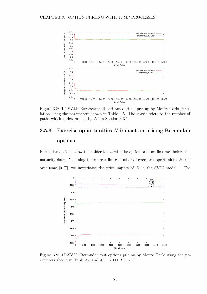
CHAPTER 3. OPTION PRICING WITH JUMP PROCESSES
7.85 7.9
7.95 8
8.05 8.1
8.15 8.2
8.25 8.3
8.35
0 500000 1e+06 1.5e+06 2e+06 2.5e+06 3e+06 3.5e+06 4e+06 4.5e+06 5e+06E
urop
ean
Cal
l Opt
ion
Pric
eNo. of Paths
Monte Carlo methodExact Price(8.2121)
3.25
3.3
3.35
3.4
3.45
3.5
3.55
3.6
3.65
0 500000 1e+06 1.5e+06 2e+06 2.5e+06 3e+06 3.5e+06 4e+06 4.5e+06 5e+06
Eur
opea
n P
ut O
ptio
n P
rice
No. of Paths
Monte Carlo methodExact Price(3.3350)
Figure 3.8: 1D-SVJJ: European call and put options pricing by Monte Carlo simu-lation using the parameters shown in Table 3.5. The x-axis refers to the number ofpaths which is determined by N∗ in Section 3.3.1.
3.5.3 Exercise opportunities N impact on pricing Bermudan
options
Bermudan options allow the holder to exercise the options at specific times before the
maturity date. Assuming there are a finite number of exercise opportunities N > 1
over time [0, T ], we investigate the price impact of N in the SVJJ model. For
3.55
3.6
3.65
3.7
3.75
3.8
3.85
3.9
3.95
4
0 500 1000 1500 2000 2500 3000 3500 4000 4500 5000
Ber
mud
an p
ut o
ptio
n pr
ices
No. of runs
N=2N=10N=50
N=100
Figure 3.9: 1D-SVJJ: Bermudan put options pricing by Monte Carlo using the pa-rameters shown in Table 3.5 and M = 2000, J = 6
81

CHAPTER 3. OPTION PRICING WITH JUMP PROCESSES
different exercise opportunities N , Fig 3.9 demonstrates the expected relationship for
put option prices and N ; the more exercise opportunities, the more expensive the
option. We find significant differences between the prices given by N = 2, 10 and 50
(increased by 6.20% and 2.70% respectively) but a slight difference between N = 50
and N = 100 (increased by 0.42%). This implies that when N is large enough, the
estimated price changes slightly and tends to a limit, which can be regarded as an
estimate to an American option with infinite exercise opportunities.
3.5.4 Sensitivity of Bermudan options to the choice of nu-
merical parameters
For pricing Bermudan options with early exercise, i.e. N > 1, we examine several
numerical parameters affecting the option prices, which are the number of sample
paths for least squares calculations M , the highest order of Chebyshev polynomials
J and the size of time steps ∆t.
1. Sample Size M Impact on Option Price
As mentioned in Section 2.4, the convergence rate of standard Monte Carlo
simulations is proportional to the square root of the number of sample paths
employed in the least square algorithm, that is 1/√M for each run in the
LSM algorithm for pricing Bermudan options. Duck et al. (2005) find that
the estimated option prices, which tend monotonically to the exact value as M
increases, can be described by the following formula:
PM = Pexact +α1√M
+α2
M+O(M− 3
2 ) . (3.25)
where the estimate Pexact is more accurate than PM obtained from M sample
paths and α1 and α2 are unknown parameters. Therefore, following the extrap-
olation technique proposed in Duck et al. (2005), we use three different sample
sizes M to estimate α1, α2 and Pexact. Duck et al. (2005) and Xiao (2007) sug-
gest that a better estimate Pexact can be efficiently yielded by M = 2000, 4000
and 8000, even on high-dimensional problems.
82

CHAPTER 3. OPTION PRICING WITH JUMP PROCESSES
3.5
3.55
3.6
3.65
3.7
3.75
3.8
3.85
3.9
3.95
4
0 500 1000 1500 2000 2500 3000 3500 4000 4500 5000
Ber
mud
an p
ut o
ptio
n pr
ices
No. of runs
M=2000M=4000M=6000M=8000
M=2000, 4000, 8000M=4000, 8000, 16000
Figure 3.10: 1D-SVJJ: Bermudan put options pricing by Monte Carlo simulationusing the parameters shown in Table 3.5 and N = 100, J = 6,∆t = T/N .
In Fig 3.10, we illustrate the effects of extrapolation on option prices after
5000 runs. Without the extrapolation procedure, we find that the price of the
Bermudan option generally reduces as M rises from 2000 to 8000 and the rate
of the price changes tends to be small (reduced by 2.47%, 1.03% and 0.59%
respectively). This implies that the option price converges to a limit which is
lower than those estimates PM and the limit can be obtained with sufficiently
large M . Using the extrapolation procedure, we also gain two fluctuating lines
for M = 2000, 4000, 8000 and M = 4000, 8000, 16000. As anticipated, the prices
vary considerably during the early runs because of the small sample sizes but
tend to be consistent after sufficient runs. The extrapolated values are some-
what lower than the other estimates PM , which are consistant with the limit
suggested by PM . Therefore, we can reasonably conclude that the extrapolation
procedure is an efficient way to obtain an accurate estimate of the option price.
Compared with two different settings of M for the extrapolation, the estimated
prices are numerically equal so that M = 2000, 4000, 8000 is a better choice for
the extrapolation in the SVJJ model.
2. ∆t and J Impact on Option Prices
Moreover, to check the reliability of results by the method used above, we con-
83

CHAPTER 3. OPTION PRICING WITH JUMP PROCESSES
3.4
3.5
3.6
3.7
3.8
3.9
4
0 500 1000 1500 2000 2500 3000 3500 4000 4500 5000B
erm
udan
put
opt
ion
pric
esNo. of runs [a]
∆t=0.01∆ t=0.005
∆ t=0.0025∆ t=0.00125
∆ t=0.001
3.4
3.5
3.6
3.7
3.8
3.9
4
0 500 1000 1500 2000 2500 3000 3500 4000 4500 5000
Ber
mud
an p
ut o
ptio
n pr
ices
No. of runs [b]
J=6J=8
J=10J=12
Figure 3.11: 1D-SVJJ: Bermudan put options pricing by Monte Carlo simulationusing the parameters shown in Table 3.5 and N = 100, [a] using J = 6,M =2000, 4000, 8000 and [b] using ∆t = T/N,M = 4000, 8000, 16000
sider another two parameters, time steps ∆t and the highest order of Chebyshev
polynomials J and show them in Fig 3.11. For pricing the Bermudan option
with N = 100 and T = 1, Fig 3.11 shows that the choice of ∆t and J has
no significant impact on the option prices. Therefore the optimal parameter
setting for the algorithm of pricing Bermudan option with the extrapolation
technique is presented in Table 3.6.
Parameter Value∆t 0.01J 6M 2000, 4000, 6000
Table 3.6: The optimal parameter setting is used in pricing a Bermudan put withthe extrapolation procedure.
In Section 3.3, we recommend using ∆t = T/N because for the 1D MJD model,
SDE (3.1) has an analytic solution. Thus it can be exactly simulated, regardless of
the choice of ∆t. However, for the SVJJ model, the discretization error is introduced
by the volatility process (3.24) if ∆t is too large. Therefore, the accuracy of the
estimated option price in the SVJJ model can be increased by reducing the value of
∆t.
84
CHAPTER 3. OPTION PRICING WITH JUMP PROCESSES
3.6 Pricing multi-dimensional Bermudan put op-
tion using the SVJJ model
Based on the discussions of Section 3.4 and Section 3.5, we consider an evaluation of
a complex option under multiple assets following the SVJJ model. As described in
Section 3.4, the times of jumps across assets are different over the same time horizon,
while in Section 3.5 jumps are assumed to occur simultaneously in the processes of the
asset price and its volatility. By combining Eq (3.12) with Eq (3.18) and Eq (3.19),
the SVJJ model with multiple assets can be expressed in term of xp = log Sp, as
follows:
dxp = (r − λpκxp −1
2vp)dt+
√vpdWxp + Jxpdqp , (3.26)
dvp = κvp(θvp − vp)dt+ σvp
√vpdWvp + Jvpdqp , (3.27)
where r, λp, κvp , θvp and σvp are known constant for p = 1, · · · , P . The expectation
of jump sizes in the asset prices κxp is expressed as:
κxp = (exp(µxp +1
2δ2xp
)− 1)/(1− ρ(J)xpvp
µvp) ,
with the correlation coefficient ρ(J)xpvp for jump sizes between xp and vp.
The correlated intensity of jump-arrivals is governed by two independent Poisson
random variables:
ξ∗p ∼ Poisson(λpdt) , (3.28)
ξ∗ ∼ Poisson(λdt) , (3.29)
dqp = ξ∗p + ξ∗ .
If dqp = 0, then
Jvpdq = 0 .
If dqp 6= 0, then the magnitude of the jumps in the volatility process can be obtained
from a gamma distribution (see Abramowitz and Stegun, 1972), which is
Jvpdqp ∼ Gamma(dqp, µvp) . (3.30)
85
CHAPTER 3. OPTION PRICING WITH JUMP PROCESSES
This is because for the integer dqp, the gamma distribution represents the sum of dqp
independent exponentially distributed random variables with mean µvp .
We assume that Jxp and Jvq are independent random sizes of jumps, while Jxp
and Jxq are correlated when p 6= q. Then, the jump sizes for the log-price process
(Jx1 , · · · , JxP) can be generated from multivariate normal distribution, which is
(J1, · · · , JP ) ∼ N(µx1 , · · · , µxP; δ2
x1, · · · , δ2
xP; ΣJ) , (3.31)
where given a realised volatility jump size J∗vp, the mean µxp can be estimated by
µxp = µxp + ρ(J)xpvp
J∗vp,
and ΣJ is a P × P symmetric correlation matrix (3.15) in Section 3.4.
We also consider that the increments of Brownian motion are normally distributed
as follows:
(dWx1 , dWv1 , · · · , dWxP, dWvP
) ∼ N(0; dt; ΣW ) , (3.32)
where 0 and dt stand for mean and variance respectively, and ΣW is a 2P × 2P
symmetric correlation matrix in the following form:
∑W
=
1 ρ(W )x1v1 ρ
(W )x1x2 ρ
(W )x1v2 · · · ρ
(W )x1xP ρ
(W )x1vP
ρ(W )x1v1 1 ρ
(W )x2v1 ρ
(W )v1v2 · · · ρ
(W )xP v1 ρ
(W )v1vP
ρ(W )x1x2 ρ
(W )x2v1 1 ρ
(W )x1x2 · · · ρ
(W )x2xP ρ
(W )x2vP
ρ(W )x1v2 ρ
(W )v1v2 ρ
(W )x2v2 1 · · · ρ
(W )xP v2 ρ
(W )v2vP
......
......
......
...
ρ(W )x1xP ρ
(W )xP v1 ρ
(W )x2xP ρ
(W )xP v2 · · · 1 ρ
(W )xP vP
ρ(W )x1vP ρ
(W )v2vP ρ
(W )x2vP ρ
(W )v2vP · · · ρ
(W )xP vP 1
,
with ρ(W )xivj = ρ
(W )xixjρ
(W )xjvj for i, j = 1, . . . , P .
3.6.1 Implementation
The implementation of pricing a multi-dimensional Bermudan option in the SVJJ
model is similar to the way proposed in Section 3.4.1 with the additional processes
of the volatilities. Let N be the number of possible exercise times during the option
86
CHAPTER 3. OPTION PRICING WITH JUMP PROCESSES
life T , and V be the payoff function of the option. Therefore, following the procedure
in Section 3.4.1, in the discrete-time framework with N time steps of equal size
∆t = T/N , we derive the discrete form of Eq (3.27) and Eq (3.27) as follows:
xpj(ti+1) = xp
j(ti) + (r − λpκpx −
1
2vp
j (ti))∆t+√vp
j (ti)Zpx(ti)
√∆t
+Jpx(ti)ξ
p(ti) , (3.33)
vpj (ti+1) = vp
j (ti) + κpv(θ
pv − vp
j (ti))∆t+ σpv
√vp
j (ti)Zpv (ti)
√∆t
+Jpv (ti)ξ
p(ti) , (3.34)
for i = 0, · · · , N−1 and j = 1, · · · ,M . The number of realized jumps during the time
interval [ti, ti+1] is ξp(ti) in the p-th asset and volatility processes, which is estimated
by the sum of two random numbers from the Poisson distributions (3.28) and (3.29);
according to the expressions (3.30) and (3.31) we can evaluate the magnitudes of
the jumps occurring in the interval: Jpv (ti)ξ
p(ti) and Jpx(ti)ξ
p(ti) respectively; the
correlated random variables Zpx(ti) and Zp
v (ti) for p = 1, · · · , P can also be modelled
from a multivariate normal distribution (3.32). Therefore, the log-price process x(ti)
can be directly generated by Eq (3.34). Following the same algorithm as described
in Section 3.4.1, the Bermudan option can be estimated by averaging the results
obtained from Mrun times of the LSM procedure.
3.6.2 Numerical results
In this section, we illustrate the algorithm in Section 3.6.1 by pricing a two-dimensional
Bermudan option in the SVJJ model. The parameters used here are given by Ta-
ble 3.7 and the payoff function of the option is V , which is
V = max(K1 − S1, K2 − S2, 0) .
1. Exercise opportunities N Impact on Option Price
We investigate how option prices change with respect to the number of exercise
opportunities, N . Fig 3.12 shows that the option prices calculated by our algo-
rithm with sample size M = 2000 are convergent after a number of runs. From
87

CHAPTER 3. OPTION PRICING WITH JUMP PROCESSES
Parameter ValueSp(t0) 100Kp 100r 0.05T 1.0
σp0 =
√vp
0 0.0870κp
v 3.46θp
v 0.008σp
v 0.14λp = λ 0.235µp
x −0.10δpx 0.0001µp
v 0.0500
ρ(J)xv −0.38
ρ(J)xx 0.2
ρ(W )xx = ρ
(W )vv 0.2
ρ(W )xpvp −0.82p 1, 2
Table 3.7: This set of parameters is used to demonstrate the numerical approach ofpricing a Bermudan put on 2D SVJJ model
Fig 3.12, we can see that the Bermudan option (N ≥ 2) prices are significantly
higher than the observed European option price (N = 1). The Bermudan op-
tion becomes more expensive as N increases, whilst the increment of the option
prices tends to be small when N is large enough, where an approximation for
the corresponding American price is obtained.
2. Sample Size M Impact on Option Price
Fig 3.13 provides the results of option prices for different sample sizes M with-
out extrapolation and then shows the estimated price by the extrapolation
procedure with the optimal parameters in Table 3.6. Similar to the results in
Fig 3.10, the estimate of the put option value reduces as M increases. Com-
pared with the raw method with a single value M , the extrapolated method
(M = 2000, 4000, 8000) produces the lowest price that is more variable dur-
ing early runs, but is shown to be convergent as the number of runs increases,
which implies that the extrapolation technique also performs well when solving
a multi-dimensional problem to achieve an accurate estimate effectively.
88

CHAPTER 3. OPTION PRICING WITH JUMP PROCESSES
6.8
7
7.2
7.4
7.6
7.8
0 500 1000 1500 2000 2500 3000 3500 4000 4500 5000
Ber
mud
an p
ut o
ptio
n pr
ices
No. of runs
N=1N=2N=5
N=10N=20N=50
N=100
Figure 3.12: 2D-SVJJ: Pricing Bermudan put options on the two underlyings withrespect to the number of exercise opportunities N using parameter list showed inTable 3.7, J = 6, ∆t = 0.01 and M = 2000.
3.7 Comparison of jump diffusion models
Jump diffusion models are considered as an approach to relax the Black-Scholes
model. We have discussed different jump diffusion models in this chapter, which
are derived from the fundamental Merton (1976) jump model. More specifically, we
illustrate a LSM algorithm to price Bermudan options under the MJD model and the
SVJJ model and extend it to a multi-dimensional problem to price Bermudan basket
options. In this section, we compare different models in terms of option pricing under
certain parameter settings as seen in Table 3.8. The parameters listed in Table 3.8
are based on those parameters used to price two-dimensional options in the SVJJ
model in Section 3.6.2, and the values of the parameters for the other models are
taken to make these models comparable in general. We choose the value for σp0 in
the constant volatility models, such as the BS models and MJD models, equal to the
value for the long-term level θpv in the stochastic volatility models, i.e. SVJJ models.
Also the expectation of the intensity of jumps λ in one-dimensional models equals
the sum of λp and λ in two-dimensional models, that is, λ = λp + λ.
89

CHAPTER 3. OPTION PRICING WITH JUMP PROCESSES
9.6
9.8
10
10.2
10.4
10.6
10.8
11
0 500 1000 1500 2000 2500 3000 3500 4000 4500 5000
Ber
mud
an p
ut o
ptio
n pr
ices
No. of runs
M=2000M=4000M=8000
M=2000,4000, 8000
Figure 3.13: 2D-SVJJ: Bermudan put options pricing by Monte Carlo using param-eter list showed in Table 3.7, J = 6, exercise opportunities N = 100 and ∆t = 0.01.
Parameter 1D-BS 1D-MJD 1D-SVJJ 2D-BS 2D-MJD 2D-SVJJSp(t0) 100 100 100 100 100 100Kp 100 100 100 100 100 100r 0.05 0.05 0.05 0.05 0.05 0.05T 1.0 1.0 1.0 1.0 1.0 1.0
σp0 =
√vp
0
√0.008
√0.008 0.0870
√0.008
√0.008 0.0870
κpv n/a n/a 3.46 n/a n/a 3.46θp
v n/a n/a 0.008 n/a n/a 0.008σp
v n/a n/a 0.14 n/a n/a 0.14λ (λp = λ) n/a 0.47 0.47 n/a 0.235 0.235µp
x n/a −0.10 −0.10 n/a −0.10 −0.10δpx n/a 0.0001 0.0001 n/a 0.0001 0.0001µp
v n/a n/a 0.0500 n/a n/a 0.0500
ρ(J)xv n/a n/a −0.38 n/a n/a −0.38
ρ(J)xx n/a n/a n/a n/a 0.2 0.2
ρ(W )xx = ρ
(W )vv n/a n/a n/a 0.2 0.2 0.2
ρ(W )xv n/a n/a −0.82 n/a n/a −0.82p 1 1 1 1, 2 1, 2 1, 2
Table 3.8: Parameter setting for different jump models and Black-Scholes models,which are one-dimensional Black-Scholes model (1D-BS), one-dimensional Mertonjump diffusion model (1D-MJD) and one-dimensional stochastic volatility jump dif-fusion model (1D-SVJJ), and their two-dimensional versions: 2D-BS, 2D-MJD, and2D-SVJJ.
Table 3.9 shows the resulting prices of put options with and without extrapola-
tion with respect to the number of exercise opportunities N . From Table 3.9, we
90

CHAPTER 3. OPTION PRICING WITH JUMP PROCESSES
Model N M ext M = 2000 M = 4000 M = 8000
1D-BS 1 1.56989130836 1.57172972200 1.57156537756 1.571262111272 1.83017513710 1.83464969367 1.83426412149 1.8335289832410 2.01329588241 2.04481473990 2.03542299443 2.0288620704550 2.06569368846 2.11020323982 2.08736672051 2.07611884962100 2.05948412345 2.12467582135 2.09925653993 2.08444493126
1D-MJD 1 2.41324307718 2.40023758711 2.39773717863 2.399123937012 2.69694670509 2.70383435596 2.70047940248 2.6987758957510 2.94884600029 2.96990521753 2.95250901041 2.9458220869950 3.00476323316 3.05435747793 3.02230512143 3.00840395206100 3.00527852296 3.07017245759 3.03579333146 3.01916968461
1D-SVJJ 1 3.36058142049 3.35158677589 3.35260028812 3.354127428582 3.60991595365 3.60668419642 3.59919491046 3.5981171084410 3.72388085676 3.83187905320 3.77823298342 3.7513065488950 3.65536581505 3.93120728964 3.84510310739 3.78687429867100 3.67918799555 3.95401450826 3.85309003471 3.79194048088
2D-BS 1 2.75862314578 2.74876260006 2.74931149457 2.750869217832 3.07473929655 3.08897843215 3.07641938973 3.0717330537510 3.29338320608 3.39139104304 3.34660584631 3.3229776129550 3.33725977524 3.51448392431 3.43408620691 3.39148141871100 3.32371962082 3.53340717165 3.44758088882 3.39909765279
2D-MJD 1 5.03082461948 5.05202123532 5.05524692936 5.052810819952 5.20520584521 5.25421502592 5.23346230660 5.2219870493610 5.32698175737 5.52402193573 5.44764046257 5.4029654754950 5.35169616022 5.63126355620 5.51746505624 5.45295491796100 5.34304283637 5.64071551573 5.52322462010 5.45529830428
2D-SVJJ 1 6.84287868988 6.83576925240 6.83958954113 6.841421901842 6.92155965963 7.01529939522 6.98068726802 6.9597909953310 6.95980393695 7.34388227010 7.19910501027 7.1128736883650 6.86741732955 7.48826871869 7.27264749177 7.13706929262100 6.82807813448 7.49256206851 7.26917148315 7.12559435893
Table 3.9: comparison of put prices in different jump models. The results shownin the column M ext are given by the simulation with the extrapolation scheme forM = 2000, 4000 and 8000. All the results are obtained after Mrun = 5000 runs.
can clearly see that the approximated option prices in two-dimensional models are
generally significantly higher than the corresponding option prices estimated in one-
dimensional models, because there are more chances to profit from holding a basket
91
CHAPTER 3. OPTION PRICING WITH JUMP PROCESSES
put option with payoff u = max(K1 − S1, K2 − S2, 0) than in holding a standard put
options whose payoff is u = max(K1 − S1, 0). Both jump models: MJD and SVJJ
produce higher prices than the standard Black-Scholes model prices. Compared with
the MJD models, the SVJJ models produce higher option values due to a stochastic
volatility process. With respect to N , there is an increase in the option price as the
number of exercise opportunities arises in all the models, which is consistent with the
results without extrapolation in Table 3.9.
As for the extrapolation method, in each jump model we find that the option
prices evaluated by the extrapolation technique are lower than the corresponding
prices generated without using extrapolation. When pricing Bermudan options with
N > 1, there is an obvious advantage with the extrapolation method: the prices
using extrapolation are more accurate than the prices given by the raw algorithm.
This advantage increases as the number of exercise opportunities N increases.
92
Chapter 4
Feedback Models with Illiquidity
Futures and options are the tail wagging the dog. They have also esca-
lated the leverage and volatility of the markets to precipitous, unacceptable
levels.
– John Shad
Wall Street Journal. 1988
4.1 Background
As mentioned in Section 3.1, the simple Merton (1976) jump diffusion model seems
not to fit the quoted option prices significantly better than the standard Black-Scholes
model. In this chapter, we discuss another kind of model, concerning market liquidity,
to relax the restrictive Black-Scholes assumptions in a different way.
In the past, most academic discussion concerning asset pricing models has been
based on complete markets, with sufficient liquidity to allow the purchase or sale of
any amount of the underlying asset at any time, without causing significant movement
in the asset’s price. The generalised asset pricing model described in the seminal
paper by Black and Scholes (1973) may be expressed as,
dS = µ(S, t)Sdt+ σ(S, t)SdW , (4.1)
where dW is a Wiener process, µ(S, t) is the function of expected return and σ(S, t) is
93

CHAPTER 4. FEEDBACK MODELS WITH ILLIQUIDITY
the volatility function. In the original model, it is assumed that µ and σ are constants
in a risk-neutral world, and µ is replaced by the risk-free rate, r
dS = rSdt+ σSdW . (4.2)
Through the application of Ito’s lemma and a hedging argument, now studied in
textbooks (e.g. see Hull, 2009; Wilmott et al., 1995) the Black-Scholes-Merton partial
differential equation (PDE) is derived, from which, when boundary conditions have
been applied, a huge range of financial options can be priced and upon which much
of the literature on option pricing is based. For options maturing under one year
on stocks or stock indices, this modelling approach has been successful as a first
approximation in practical option pricing.
The assumptions of constant volatility and constant risk-free interest rate were
both relaxed in favour of stochastic modelling in other strands of the literature. Con-
stant volatility is known to be too restrictive an assumption, leading to the practical
observation of “volatility smiles”. Similarly, constant interest rate becomes inappro-
priate for all but short-term options (perhaps under a year to maturity). However, a
less well researched area by far is the assumptions of perfect elasticity for the supply
and demand of underlying traded assets. Financial models which are based on the
assumption that an investor trading a large number of assets cannot impact the price
movement, may fail when market liquidity vanishes. The literature on illiquidity can
roughly be divided into two approaches: (i) studies on price impact due to large
traders, and (ii) studies on price impact due to immediacy provision by market mak-
ers. In the models falling into the first category, larger traders can move the price by
their actions on pricing and hedging. Jarrow (1992) finds conditions on the economy
consisting of a money market and a stock market that exclude market manipulation
strategies. Jarrow (1994) develops the standard theory of pricing and hedging of
derivative securities, with a feedback effect from the large trader’s position. In a
discrete-time framework, he denotes the impact of the large trader’s activities on the
price process via a reaction function, which is an exponential function with respect
94

CHAPTER 4. FEEDBACK MODELS WITH ILLIQUIDITY
to the large trader’s share and option holdings. He demonstrates that market ma-
nipulation strategies exist using the derivative securities if there are no additional
conditions on the price process. The conditions shown in his model are (i) there is
a limit to the number of the total holdings imposed on the large trader’s position,
and (ii) the stock, money market fund, and derivative security markets have to be
synchronous to prevent manipulation strategies. Jarrow’s results have been extended
to the continuous time framework by Frey (1996), Frey and Stremme (1997), Platen
and Schweizer (1998) and Bank and Baum (2004). Frey (1996) focuses on the ad-
ditional assumption in Jarrow (1994): the synchronous market condition to derive
a full pricing theory in a finitely-elastic market. Moreover, he finds that the cost
of hedging derivatives is influenced by the position held by larger traders. Frey and
Stremme (1997) consider the feedback effects on market volatility and provide the
tracking error, i.e. the discrepancy between the cost of the standard Black-Scholes
hedging portfolio and the actual modelling value of a European call option. The
tracking error is shown to be largest for ATM options, and to vanish for DITM and
DOTM options. Frey and Patie (2002) present more details on the performance of
different hedging strategies, and show that a optimal hedging portfolio is more accu-
rate than the standard Black-Scholes hedge as the tracking error is relatively small.
The feedback effect is also used to explain the ‘smile pattern’ and ’skewness pattern’
of the implied volatility of the underlying assets in Platen and Schweizer (1998) and
Frey and Patie (2002). Sircar and Papanicolaou (1998) derive a different nonlinear
PDE that depends on the exogenous income process of the reference traders and the
relative size of the program traders. Schonbucher and Wilmott (2000) analyze the
influence of dynamic strategies on pricing, hedging and replication of an option in a
general equilibrium model. Liu and Yong (2005) examine whether the put-call parity
is satisfied in the modified PDE and deduce a special form of put-call parity due to
the initial transaction costs considered. Rather than using the reaction function of
the direct feedback effect in Jarrow (1994), Cuoco and Cvitanic (1998) and Cvitanic
and Ma (1996) study a diffusion model for price dynamics by making the drift and
volatility coefficient depend on the large traders’ trading strategy.
95
CHAPTER 4. FEEDBACK MODELS WITH ILLIQUIDITY
The second approach involves the price impact due to provisions of immediacy
by market makers, which is studied in Cetin, Jarrow and Protter (2004), Rogers and
Singh (2006) and Cetin and Rogers (2006). These models capture the features of a
short-term price impact of large traders using the equalisation of supply and demand
in the short-term market, i.e. the price impact disappears instantaneously when there
are no large volume trades. Bakstein and Howison (2003) adopt a similar approach
to Rogers and Singh (2006), but the former study leads to feedback effects, which
the latter study was trying to avoid. Another model in this category is the work of
Cetin, Jarrow, Protter and Warachka (2006), who modelled the illiquidity cost as a
stochastic supply curve with the underlying asset price depending on order flow.
The study presented in this thesis is based on the first approach to study the price
impact, where the volume traded by ‘large traders’ cannot be absorbed by the market
without price changes and there exists feedback effects from trading strategies. In
particular, we illustrate the effects on pricing derivatives.
4.2 Modelling framework
We propose an asset pricing model in an illiquid market, which is also employed in
Liu and Yong (2005) and Glover (2008). Rather than working on a modified PDE for
pricing derivatives as used in these previous works, we focus on deriving a modified
stochastic differential equation of the underlying asset. The asset model presented
here is as follows:
dS = µSdt+ σSdWS + λSdΦ , (4.3)
where S is the underlying price, µ and σ are the constant drift and volatility respec-
tively and WS is a standard Brownian motion. Φ represents the number of shares
held by a single ‘large trader’, which is a smooth, differentiable function of S and t.
The ‘large trader’ can be interpreted as a market maker who can take arbitrarily large
positions or a group of small traders who follow the same trading strategies. λS can
be interpreted as some function specifying how illiquid the market is, where λ is the
illiquidity coefficient. The term λSdΦ is considered as the price impact made by the
96

CHAPTER 4. FEEDBACK MODELS WITH ILLIQUIDITY
trader when she follows some strategy in buying or selling the asset. Compared with
the model used in Glover (2008), our model includes an extra ‘S’ in the last term on
the right of Eq (4.3) to model the impact of the market illiquidity as the market value
of trading shares, rather than just the number of the shares. With the additional S,
the amount of the trading shares dΦ has been mapped to the corresponding impact
on the share price movement. In addition, the quantity 1λS
is referred to as the ‘mar-
ket depth’, which is the size of a order needed to cause one unit of asset price change
in the market.
As Φ(S, t) is smooth and differentiable, using Ito’s Lemma we obtain
dΦ(S, t) = Φtdt+ ΦSdS +1
2ΦSS(dS)2 .
Substituting this into Eq (4.3), we obtain, as dt→ 0,
(1− λSΦS)dS = (µS + λSΦt)dt+ σSdWS +1
2ΦSSdS2 ,
and so
dS =µS + λSΦt
1− λSΦS
dt+σS
1− λSΦS
dWS +1
2
ΦSS
1− λSΦS
dS2 . (4.4)
Then squaring Eq (4.4) gives
dS2 =σ2S2
(1− λSΦS)2dt+ o(dt) (4.5)
as dt→ 0. Substituting Eq (4.5) into Eq (4.4), we arrive at an adjusted price model:
dS = µ(S, t)dt+ σ(S, t)dWS , (4.6)
where
σ(S, t) =σS
1− λSΦS
,
µ(S, t) =µS + λSΦt
1− λSΦS
+1
2
λσ2SΦSS
1− λSΦS
. (4.7)
In the case of delta hedging, we can identify the number of shares Φ(S, t) to
hedge a derivative V (S, t). Note that the SDE (4.6) is different from the one shown
in Glover (2008) due to involving SΦS term instead of ΦS. Then, following a similar
analysis in Glover (2008), we discuss two kinds of feedback models for different trading
97

CHAPTER 4. FEEDBACK MODELS WITH ILLIQUIDITY
strategies. First, we assume that the price taker who does not know the existence
of the market illiquidity applies delta hedging as in the derivation of the standard
Black-Scholes formula, i.e. ∆ = V BSS which has an analytical form: ∆ = N(d1) for
call options whilst ∆ = 1−N(d1) for put options1, where N(·) is the standard normal
distribution function. We call this case ‘first-order feedback’ which is used to model
the price impact of the sub-optimal hedging strategy of the price taker. For more
complicated cases, the hedging strategy taken by the market maker who realises the
illiquidity impact on the underlying price follows the modified SDE (4.6), i.e. ∆ = VS
for which we need to appeal to numerical methods for solution. This case, called ‘full
feedback’, is subject studied in Chapters 7 and 8. Therefore, under a risk-neutral
measure, instead of Eq (4.6) one of many simple dynamic of the asset movement is
given by
dS = rSdt+σS
1− λSV BSSS
dWS , (4.8)
in the case of the first-order feedback SDE, or for the full feedback SDE,
dS = rSdt+σS
1− λSVSS
dWS , (4.9)
where r is the instantaneous risk-free interest rate. The second derivative of V with
respect to S affects the modified volatility (V BSSS denotes the value of the ‘gamma’ in
Black-Scholes model) together with the illiquidity coefficient λ. The case of λ = 0
implies that the market is perfectly liquid and vanilla option prices can be calculated
by the standard Black-Scholes formula. Rather than the non-linear PDE applied in
Frey and Patie (2002), we have not put any constraints on the volatility term in
Eq (4.8) and Eq (4.9), which might cause numerical problems when the volatility
term tends to zero or infinity. To deal with these circumstances, we will include
additional constrains on the simulation algorithm of specific models in later chapters.
In the following chapters, we will illustrate how to use the Monte Carlo method to
simulate the path following the stochastic processes (4.8) and (4.9) and analyse the
results of option pricing. Chapter 5 investigates the first-order feedback model (4.8)
with a constant illiquidity λ while a stochastic illiquidity λ is studied in Chapter 6;
1where d1 is defined as log(S/K)+(r+ 12 σ2)(T−t)
σ√
T−t.
98

CHAPTER 4. FEEDBACK MODELS WITH ILLIQUIDITY
Chapters 7 and 8 consider the full feedback model (4.9) with constant λ and stochastic
illiquidity λ respectively.
99

Chapter 5
First-Order Feedback Model with
Constant Illiquidity
We start with the simplest model, which is first-order feedback with constant illiq-
uidity λ. In such an illiquid market, a trader does realize that the market is illiquid
but hedges his position as in an original Black-Scholes model. The price impact of
his trade volume is related to V BSSS in a modified SDE. Recall the effective dynamic
process (4.8) of the underlying using a risk-neutral measure:
dS = rSdt+σS
1− λSV BSSS
dWS ,
and for pricing a European call option with a standard payoff function (S −K)+ at
maturity,1 the corresponding V BSSS (the Gamma) is derived from the Black-Scholes
formula (for more details of the derivation, see Higham, 2004), which is
V BSSS =
e−12d21
σS√
2π(T − t),
d1 =log(S/K) + (r + 1
2σ2)(T − t)
σ√T − t
, (5.1)
and we notice the same form of V BSSS given by a European put option. The modified
volatility term in SDE (4.8) can capture the underlying price dynamics affected by
the delta hedging of large investors who are assumed to trade the number of stocks
V BSS raised from the standard Black-Scholes formula. We study in detail how the
1Denoted as max(S −K, 0)
100
CHAPTER 5. FIRST-ORDER FEEDBACK - CONSTANT ILLIQUIDITY
modified volatility term has an impact on option pricing in Section 5.2, particularly
for changes in the denominator of the volatility term.
The rest of the chapter is organised as follows: Section 5.1 introduces how to
use Monte Carlo simulation to evaluate option prices under the stock process given
by (4.8). Section 5.2 presents results we find using this model. In Section 5.3 we
compare our model with that proposed in Glover (2008).
5.1 Implementation
In this section, we illustrate how to apply Monte Carlo simulation for pricing a
European call option V (0) at time t = 0. The first step is to apply the Euler scheme
to approximate the SDE (4.8) at discrete times t = 0, t1, t2, · · · , T . As the value of
V BSSS (S, ti) can be calculated in time, the underlying price S(T ) at terminal time T is
easily obtained. The payoff of a call option V (T ) is estimated by the standard payoff
function (ST −K)+ and the value of the option V (0) at initial time t = 0 is found by
discounting the payment V (T ) via the factor e−rT with a constant risk-free interest
rate r. The process has to be repeated to obtain a sufficient number of the V (0)
values, and then we treat the average value of these V (0) as a reasonable estimator
of the call price. The following algorithm describes the procedure in detail:
1. Divide the life of option [0, T ] into N small time periods [ti, ti+1] with equal
duration ∆t, i.e. ti+1 = ti + ∆t, where i = 0, · · · , N − 1 and t0 = 0, tN = T .
2. Generate M independent paths of the underlying price Sj(ti) for j = 1, · · · ,Mby simple Euler discretization. The approximation of SDE (4.8) is given by
Sj(ti+1) = Sj(ti) + rSj(ti)∆t+σSj(ti)
1− λSj(ti)V BSSSj
(Si, ti)(Wj(ti+1)−Wj(ti)) ,
for each path j. Because Brownian motion has independent normally dis-
tributed increments, the simulation of Wj(ti+1)−Wj(ti) is equal to a standard
normal random variable Zj(ti) multiplied by the square root of the time in-
crement ∆t. Therefore the approximation described above can be rewritten
101

CHAPTER 5. FIRST-ORDER FEEDBACK - CONSTANT ILLIQUIDITY
as:
Sj(ti+1) = Sj(ti) + rSj(ti)∆t+σSj(ti)
1− λSj(ti)V BSSSj
(Si, ti)Zj(ti)
√∆t . (5.2)
Hence, for pricing the option by this algorithm, we need NM standard normal
random numbers in total.
3. Estimate the value of V BSSSj
(ti) at time ti by the corresponding Black-Scholes
formula for Greeks as follows:
V BSSSj
(Si, ti) =e−
12d21
σSj(ti)√
2π(T − ti), (5.3)
d1 =log(Sj(ti)/K) + (r + 1
2σ2)(T − ti)
σ√T − ti
.
Therefore, the process to estimate of the terminal price Sj(T ) is quite straight-
forward.
• The formula (5.3) implies that the Gamma (i.e. V BSSSj
(Si, ti)) increases for
options being in-the-money and reaches a peak for at-the-money options,
whilst the Gamma decreases for options being away from the money. The
Gamma also increases as expiration approaches, and for a near-the-money
option, the value V BSSSj
(Si, ti) becomes large close to expiry. For a discrete
model, the maximum value
[V BS
SSj(Si, ti)
]max
=e(r+σ2)∆t
σK√
2π∆t
occurs when Si = Ke−(r+ 32σ2)∆t and ti = T − ∆t. This suggests that
an extremely large value of V BSSSj
(ti) is possible during the period close to
maturity T .
• Moreover, we find that for some values of V BSSSj
(Si, ti), the denominator of
the volatility term, 1 − λSV BSSS in SDE (4.8) can be close to zero, which
leads to a high variance of the underlying. The affected underlying prices
could jump down to a negative value or jump up to a high level. Either
of these is undesirable, because negative stock prices cause arbitrage op-
portunities (and it also leads to problems in calculating d1 to simulate the
102

CHAPTER 5. FIRST-ORDER FEEDBACK - CONSTANT ILLIQUIDITY
following price), while abnormally high underlying prices lead to an unre-
alistic price or an overpricing of call options. Compared with the jumps
described in Chapter 3, the jumps we discuss here are caused by abrupt
changes in the volatility term rather than those jumps modelled by the
additional term of jump individually. Thus, different from those well con-
trolled jumps, we need to take some measure to remove the paths affected
by those abnormal jumps from the simulation.
To implement the algorithm, for each path j, the price Sj(ti) has to be
checked at each time point ti. If the current price Sj(ti) satisfies:
Sj(ti) < 0 or Sj(ti) > S ,
where S denotes the highest underlying price which can be accepted, then
we interrupt to simulate the j-th path by setting the related option price
Vj(0) = 0, then carry on the next simulation of the (j + 1)-th sample
path. In addition, the total number of abandoned paths occurring in
the algorithm will be referred to as m which is subtracted from the total
number of samples M when we compute the average value of the option
price. We call this procedure a price cap and floor scheme, and one of
its applications in real markets is called as ‘circuit breakers’. This is a
trading restriction to halt trading when the prices rise or fall too far, too
soon, such as the May 6, 2010 ‘Flash Crash’ that the Dow Jones Industrial
Average (DJIA) fell almost 1, 000 points within a few minutes.
In in Fig 5.4, we show that the results of option prices obtained from the
algorithm without the capping scheme are problematic as the estimated
prices are hard to converge as the number of sample paths increases.
4. Calculate the terminal payoff Vj(T ) using (Sj(T ) − K)+ and multiply the
discount factor e−rT to compute the discounted payoff Vj(0) at time 0 for
j = 1, · · · ,M .
5. Take the average of the discounted payoff on M − m live paths (those not
103

CHAPTER 5. FIRST-ORDER FEEDBACK - CONSTANT ILLIQUIDITY
abandoned) as the estimator of the option price V (0), i.e.
V (0) =1
M −m
M∑j=1
Vj(0) .
We assume that the law of large number holds in the presence of caps and
floors, which implies V (0) → V (0).
Notice that the algorithm described above does not assume any particular type of
financial derivative.
5.2 Numerical results
5.2.1 Denominator of the volatility term
As the Gammas, V BSSS , can be evaluated directly by the analytic form Eq (5.1), we
are concerned with the value of the denominator of the volatility term in Eq (4.8), in
particular SV BSSS . In Fig 5.1, the value of SV BS
SS is plotted with respect to the varying
spot price S and current time t with time-step ∆t = 0.2. The value of Gamma V BSSS
0 0.5 1 1.5 2 2.5 3 3.5 4 4.5
P
0 1 2 3 4 5 6 7 8 9 10t 0
0.2 0.4
0.6 0.8
1 1.2
1.4 1.6
1.8 2
underlying S
0 0.5
1 1.5
2 2.5
3 3.5
4 4.5
S*Gamma
Figure 5.1: Value of SV BSSS with respect to S & t, assuming K = 1, r = 0.04, σ =
0.2, T = 10 and ∆t = 0.2
is extremely small if the spot price S does not hit the strike price K, thus the value
of Gamma multiplied the spot price S is still small. If S hits close to the strike price
K, then the value of the product SV BSSS is close to the value of KV BS
SS .
104
CHAPTER 5. FIRST-ORDER FEEDBACK - CONSTANT ILLIQUIDITY
In the remaining section, we give a detailed discussion on the denominator of
volatility term as follows:
• The value of SV BSSS is positive because for call and put options in the Black-
Scholes model, the Gamma V BSSS is always positive.
• For any fixed time point t, when S → Ke−(r+ 12σ2)(T−t), the value of SV BS
SS
reaches a peak; otherwise, the value of SV BSSS decreases to zero. We can find
the value of S where the Gamma takes on the maximum value by setting the
first derivative
∂
∂S
(SV BS
SS
)= − d1e
− 12d21
SKσ2(T − t)√
2π= 0 ,
which yields the maximum value at the point S = Ke−(r+ 12σ2)(T−t):
[SV BSSS ]max =
1
σ√
2π(T − t).
• The maximum value [SV BSSS ]max increases monotonically as t increases. There
is a significant increase of the maximum function as t becomes close to T .
Thus, the peak value of P shown in Fig 5.1 is equal to 1σ√
2π∆tat position
(Ke−(r+ 12σ2)∆t, T − ∆t) and the size of the peak value is proportional to the
inverse square root of ∆t.
• As shown in Glover (2008), the denominator of the volatility term can vanish
for pairs (S, t) that satisfy the following equation:
1− λSV BSSS (t, S) = 0 , (5.4)
using the Black-Scholes formula, this can be written:
1− λS
σS√
2πτexp
(−
(log(S/K) + (r + 1
2σ2)τ
)2
2σ2τ
)= 0 ,
where τ = T − t presents time to expiry, thus S can be expressed in the explicit
form of τ :
S(τ) = K exp(− (r +
1
2σ2)τ ± σ
√τ√
2 log λ− log(2πσ2τ)), (5.5)
105
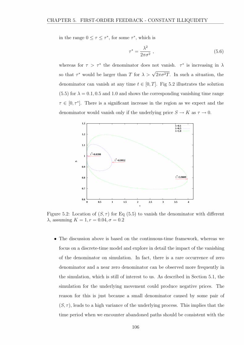
CHAPTER 5. FIRST-ORDER FEEDBACK - CONSTANT ILLIQUIDITY
in the range 0 ≤ τ ≤ τ ∗, for some τ ∗, which is
τ ∗ =λ2
2πσ2, (5.6)
whereas for τ > τ ∗ the denominator does not vanish. τ ∗ is increasing in λ
so that τ ∗ would be larger than T for λ >√
2πσ2T . In such a situation, the
denominator can vanish at any time t ∈ [0, T ]. Fig 5.2 illustrates the solution
(5.5) for λ = 0.1, 0.5 and 1.0 and shows the corresponding vanishing time range
τ ∈ [0, τ ∗]. There is a significant increase in the region as we expect and the
denominator would vanish only if the underlying price S → K as τ → 0.
0.6
0.7
0.8
0.9
1
1.1
1.2
1.3
0 0.5 1 1.5 2 2.5 3 3.5 4
S
τ
τ*=0.0398
τ*=0.9952
τ*=3.9809
λ=0.1λ=0.5λ=1.0
Figure 5.2: Location of (S, τ) for Eq (5.5) to vanish the denominator with differentλ, assuming K = 1, r = 0.04, σ = 0.2
• The discussion above is based on the continuous-time framework, whereas we
focus on a discrete-time model and explore in detail the impact of the vanishing
of the denominator on simulation. In fact, there is a rare occurrence of zero
denominator and a near zero denominator can be observed more frequently in
the simulation, which is still of interest to us. As described in Section 5.1, the
simulation for the underlying movement could produce negative prices. The
reason for this is just because a small denominator caused by some pair of
(S, τ), leads to a high variance of the underlying process. This implies that the
time period when we encounter abandoned paths should be consistent with the
106

CHAPTER 5. FIRST-ORDER FEEDBACK - CONSTANT ILLIQUIDITY
vanishing time range found in Fig 5.2. To illustrate this point, we undertake a
similar analysis to the continuous-time model and record the abandoning region
where there exist abandoned paths. The pair of (S, τ) in the abandoning region
satisfies the following inequality:
|1− λSV BSSS | ≤ ε , (5.7)
where ε denotes some small positive value. The absolute value taken here is
because either a positive or negative small value of the denominator causes
problematic simulated paths and renders the model invalid. If ε = 0, the
inequality (5.7) reduces to the form of the equation (5.4) and the solution shown
in Eq (5.5). ε also is a measure of how large the variance is. The inequality (5.7)
can be easily solved leading to:
Sin(τ) ≤ S(τ) ≤ Sout(τ) , (5.8)
or
Sin(τ) ≤ S(τ) ≤ Sout(τ) , (5.9)
where
Sin(τ) = K exp(− (r+
1
2σ2)τ + σ
√τ√
2 log λ− log(2πσ2τ(1− ε)2)), (5.10)
Sin(τ) = K exp(− (r+
1
2σ2)τ − σ√τ
√2 log λ− log(2πσ2τ(1− ε)2)
), (5.11)
Sout(τ) = K exp(− (r+
1
2σ2)τ +σ
√τ√
2 log λ− log(2πσ2τ(1 + ε)2)), (5.12)
Sout(τ) = K exp(− (r+
1
2σ2)τ −σ√τ
√2 log λ− log(2πσ2τ(1 + ε)2)
). (5.13)
Then Sin(Sout) and Sin(Sout) refer to the boundaries of the upper and lower
abandoning regions, and the subscripts ‘in’ and ‘out’ refer to the inner and
outer bounds of the abandoning region. This means that the pairs of (S, τ)
that satisfy either (5.8) or (5.9) could result in abandoned paths, otherwise
they cannot cause negative prices.
Analogously to (5.5), valid bounds (5.10)-(5.13) exist if and only if τ ∈ [0, τ ∗out]
where τ ∗out = λ2
2πσ2(1−ε)2. Comparing with the vanishing time range τ ∈ [0, τ ∗]
107
CHAPTER 5. FIRST-ORDER FEEDBACK - CONSTANT ILLIQUIDITY
where τ ∗ = λ2
2πσ2 in (5.6), the time period of abandoned paths [0, τ ∗out] is some-
what wider than the vanishing time range because τ ∗out > τ ∗ for ε > 0.
It is important to set an appropriate level of ε to define an abandoning region.
In a discrete-time stochastic underlying process S(ti) with individual time ti,
i = 0, · · · , N , we assume the negative price, S(tn+1) < 0, is observed at some
time tn+1, which is S(ti) ≥ 0 for any i ≤ n. Then, by Euler’s method, S(tn+1)
can be estimated by the prior price S(tn) > 0 and the known parameters r, σ
and ∆t:
S(tn+1) = S(tn) + rS(tn)∆t± σ
εS(tn)
√∆tZ < 0 ,
where Z is a standard normal random variable. Dividing both sides of the
inequality by S(tn) gives:
1 + r∆t± σ
ε
√∆tZ < 0 , (5.14)
then the inequality (5.14) would hold if
ε <σ|Z|√
1/∆t+ r√
∆t<
σ|Z|max√1/∆t+ r
√∆t
, (5.15)
where |Z|max is the maximum value of |Z|. The standard normal distribution
ensures the probability of the random variable Z ≤ 3.5 is 99.977%, so we can
take |Z|max = 3.5 with 99% confidence as Z follows a continuous distribution.
Notice that the range of ε given by the inequality (5.15) would lead to negative
underlying prices; therefore, a proper value ε to prevent negative prices should
be equal to ε∗, which is defined as:
ε∗ =σ|Z|max√
1/∆t+ r√
∆t. (5.16)
With ε = ε∗, the abandoning region for negative prices is determined by (5.8)-
(5.9).
To investigate how this abandoning region works for negative prices, we generate
106 sample paths which start from the price S = 1 at t0 = 0 and estimate
the price changes at the following N = 2000 discrete time points ti = i ∆t,
108
CHAPTER 5. FIRST-ORDER FEEDBACK - CONSTANT ILLIQUIDITY
i = 0, · · · , N until maturity T = 10 with the same other parameters used in
Fig 5.2. At the same time, without any caps for large prices, we only abandon
the paths that produce negative prices and record their location (S(τi), τi) with
the time left τi = T − ti, then we count the number of abandoned paths at each
τi for i = 0, · · · , N . Then setting ε∗ = 0.05 estimated by Eq (5.16) implies the
occurrence of abandoned paths if the instantaneous variance was higher than
20σ. Fig 5.3 presents the results about the location and number of abandoned
paths for λ = 0.1, 0.5 and 1.0. The abandoning region and the vanishing line
(green lines), namely the lines shown in Fig 5.2, are also indicated in the right
panel. The results from the left panel clearly suggest that abandoned paths due
to negative prices occur during the period τ ∈ [0, τ ∗ + s] for some constant s,
which is not just the vanishing time range [0, τ ∗] but also somewhat wider than
this range. In fact, s = ε∗ because the right panel of Fig 5.3 shows that all the
scattered points (S(τi), τi) (red points) leading to negative prices are located
within this estimated abandoning region between the inner and outer bounds
(blue lines) for the three cases λ = 0.1, 0.5 and 1.0. Fig 5.3 also indicates
that the abandoning region [0, τ ∗ + ε∗], i.e. [0, τ ∗out], is extended with a larger
λ, which leads to more abandoned paths than what was found in the case of
smaller λ. This is the reason why there is an increase in the total number of
abandoned paths, which are 540 (0.054%), 7702 (0.770%) and 33366 (3.337%)
for λ = 0.1, 0.5 and 1.0 respectively, although the number of abandoned paths is
a relatively small percentage of the total sample paths M = 106. For each λ, the
cumulative number of abandoned paths reaches the peak when τ approaches τ ∗
and decreases rapidly towards both sides. This can be explained by the shape
of the abandoning region which is widest around τ ∗ and becomes narrow as τ
tends to zero. Moreover, the peak time is around τ ∗ rather than τ ∗in which is
λ2
2πσ2(1+ε)2because naturally the closer points are to the vanishing lines (green
lines), the more likely they cause negative prices. Notice that Fig 5.3(a) are
somewhat different from the others becuase the abandoning region for λ = 0.1
is indeed small relative to ∆t.
109
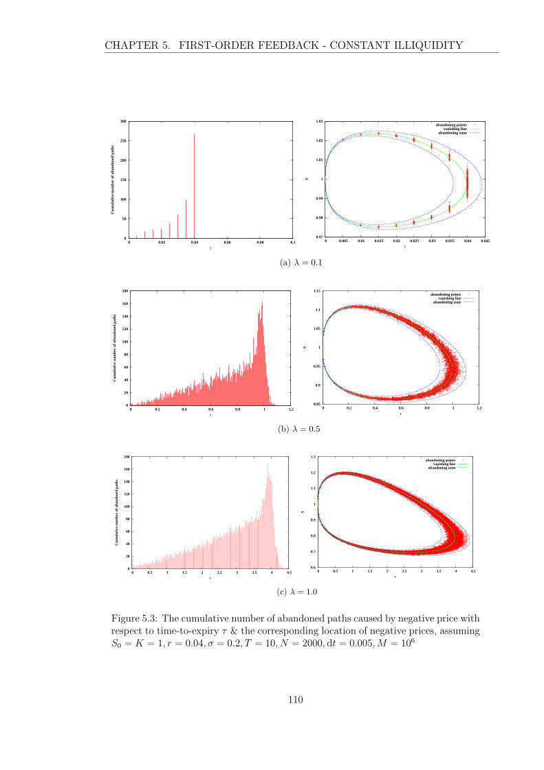
CHAPTER 5. FIRST-ORDER FEEDBACK - CONSTANT ILLIQUIDITY
0
50
100
150
200
250
300
0 0.02 0.04 0.06 0.08 0.1
Cum
ulat
ive
num
ber
of a
band
oned
pat
hs
τ
0.97
0.98
0.99
1
1.01
1.02
1.03
0 0.005 0.01 0.015 0.02 0.025 0.03 0.035 0.04 0.045
S
τ
abandoning pointsvanishing line
abandoning zone
(a) λ = 0.1
0
20
40
60
80
100
120
140
160
180
0 0.2 0.4 0.6 0.8 1 1.2
Cum
ulat
ive
num
ber
of a
band
oned
pat
hs
τ
0.85
0.9
0.95
1
1.05
1.1
1.15
0 0.2 0.4 0.6 0.8 1 1.2
S
τ
abandoning pointsvanishing line
abandoning zone
(b) λ = 0.5
0
20
40
60
80
100
120
140
160
180
0 0.5 1 1.5 2 2.5 3 3.5 4 4.5
Cum
ulat
ive
num
ber
of a
band
oned
pat
hs
τ
0.6
0.7
0.8
0.9
1
1.1
1.2
1.3
0 0.5 1 1.5 2 2.5 3 3.5 4 4.5
S
τ
abandoning pointsvanishing line
abandoning zone
(c) λ = 1.0
Figure 5.3: The cumulative number of abandoned paths caused by negative price withrespect to time-to-expiry τ & the corresponding location of negative prices, assumingS0 = K = 1, r = 0.04, σ = 0.2, T = 10, N = 2000, dt = 0.005,M = 106
110

CHAPTER 5. FIRST-ORDER FEEDBACK - CONSTANT ILLIQUIDITY
5.2.2 Put-call parity
The put-call parity condition (henceforth, PCP) formalised by Stoll (1969) should
hold in the first-order feedback model, i.e.
C +Ke−rτ = P + S , (5.17)
where C denotes the call price; P the price of the put and S the current stock price.
This can be illustrated using the linear PDE of a derivative portfolio V proposed in
Glover (2008):
∂V
∂τ+
1
2
σ2S2
(1− λSV BSSS )2
∂2V
∂S2+ rS
∂P
∂S− rV = 0 . (5.18)
Setting up a portfolio V = V1 such that V1 = P + S − Ke−rτ , then the above
PDE (5.18) yields:
∂P
∂τ+
1
2
σ2S2
(1− λSPBSSS )2
∂2P
∂S2+ rS
∂P
∂S− rP = 0 , (5.19)
with the payoff of V1 at maturity:
V1(τ = 0) =
S −K if S > K,
0 otherwise,
which is the same payoff as the call option. The PDE for the call option V2 = C is:
∂C
∂τ+
1
2
σ2S2
(1− λSCBSSS )2
∂2C
∂S2+ rS
∂C
∂S− rC = 0 , (5.20)
which shows V1 = V2 as both of them have the same payoff function and satisfy the
same form of PDE, i.e.
C = P + S −Ke−rτ .
However, following the implementation shown in Section 5.1, if we only discard the
paths with negative prices, the PCP would still fail to hold in the first-order feedback
model due to the existence of the paths with artificially high prices as discussed in
Section 5.2.1. Similar to negative prices, high prices are also caused by small values
of the denominator, where the denominator with the same sign as the standard
normal random variable leads to a positive and significant jump in the underlying,
111
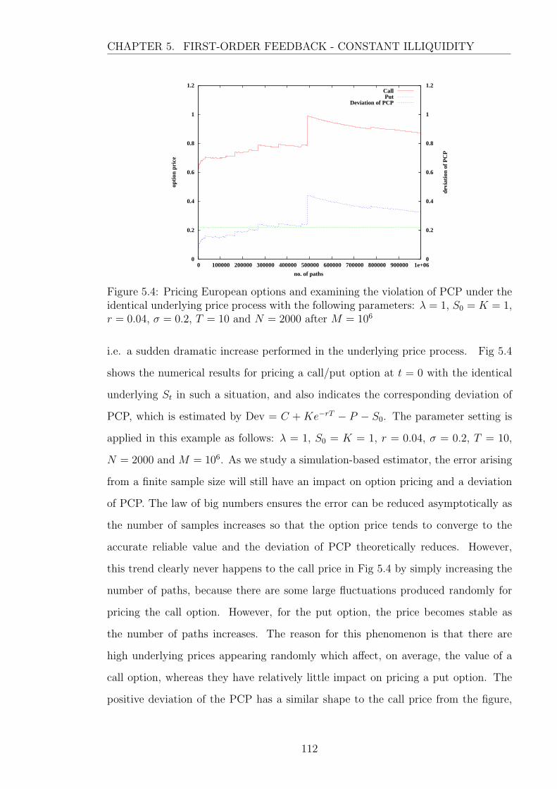
CHAPTER 5. FIRST-ORDER FEEDBACK - CONSTANT ILLIQUIDITY
0
0.2
0.4
0.6
0.8
1
1.2
0 100000 200000 300000 400000 500000 600000 700000 800000 900000 1e+06 0
0.2
0.4
0.6
0.8
1
1.2
opti
on p
rice
devi
atio
n of
PC
P
no. of paths
CallPut
Deviation of PCP
Figure 5.4: Pricing European options and examining the violation of PCP under theidentical underlying price process with the following parameters: λ = 1, S0 = K = 1,r = 0.04, σ = 0.2, T = 10 and N = 2000 after M = 106
i.e. a sudden dramatic increase performed in the underlying price process. Fig 5.4
shows the numerical results for pricing a call/put option at t = 0 with the identical
underlying St in such a situation, and also indicates the corresponding deviation of
PCP, which is estimated by Dev = C + Ke−rT − P − S0. The parameter setting is
applied in this example as follows: λ = 1, S0 = K = 1, r = 0.04, σ = 0.2, T = 10,
N = 2000 and M = 106. As we study a simulation-based estimator, the error arising
from a finite sample size will still have an impact on option pricing and a deviation
of PCP. The law of big numbers ensures the error can be reduced asymptotically as
the number of samples increases so that the option price tends to converge to the
accurate reliable value and the deviation of PCP theoretically reduces. However,
this trend clearly never happens to the call price in Fig 5.4 by simply increasing the
number of paths, because there are some large fluctuations produced randomly for
pricing the call option. However, for the put option, the price becomes stable as
the number of paths increases. The reason for this phenomenon is that there are
high underlying prices appearing randomly which affect, on average, the value of a
call option, whereas they have relatively little impact on pricing a put option. The
positive deviation of the PCP has a similar shape to the call price from the figure,
112

CHAPTER 5. FIRST-ORDER FEEDBACK - CONSTANT ILLIQUIDITY
which reveals that the failure of PCP is mainly due to the over-priced call option
obtained from the model.
Intuitively, the resolution we seek in order to make the PCP successful is to set a
maximum threshold value of the underlying price in the first-order feedback model,
which means that we need to abandon the paths whose prices exceed the maximum
value besides those paths whose prices are negative. As mentioned in the algorithm
in Section 5.1, the maximum value is called the cap of the underlying S(t), written as
S, in the subsequent discussion. Notice S can be made a function of time, t, rather
than a constant, however we study with a constant cap S over the whole option life T
for simplicity. Once S(t) > S through simulation of sample paths, we discard these
paths and restart with a new simulation. After N simulations, only live paths are
taken into account when calculating the value of the option. Fig 5.5 shows the impact
of constant caps S on pricing options compared with the situation without any caps
by setting the same parameters shown in Fig 5.4. The corresponding results for the
deviation of PCP are given in Fig 5.6. As anticipated, the estimated price tends
0.4
0.5
0.6
0.7
0.8
0.9
1
1.1
1.2
0 100000 200000 300000 400000 500000 600000 700000 800000 900000 1e+006
call
pric
e
no. of paths
noncapcap = 20cap = 10
cap = 7cap = 5
0.215
0.22
0.225
0.23
0.235
0.24
0.245
0 100000 200000 300000 400000 500000 600000 700000 800000 900000 1e+006
put
pric
e
no. of paths
noncapcap = 20cap = 10cap = 7cap = 5
Figure 5.5: European option pricing depends on the number of samples paths withvarying caps S assumed parameters: λ = 1, S0 = K = 1, r = 0.04, σ = 0.2, T = 10and N = 2000 after M = 106 runs. The left panel for a European call option and theright one for a European put option.
to converge to a limit by increasing the number of sample paths when pricing a call
option by embedding a cap to protect the underlying price S(t) from the extremely
high level, i.e. S(t) < S, as shown in the left panel of Fig 5.5. It also suggests a
decrease in S would reduce the value of a call option but increase the value of a
put option, as shown in the right panel of Fig 5.5. The small increase in the put
113

CHAPTER 5. FIRST-ORDER FEEDBACK - CONSTANT ILLIQUIDITY
price is because the put option’s payoffs taken from those paths with over-capped
price 2 are zero, in general. Therefore, eliminating those paths leads to a modest
increase in the expected value of the put option. As all of the caps employed here
are able to help to produce a convergent option price, we have to judge the four
restrictions, S = 5, 7, 10 and 20, by examining their deviation from PCP, which is
shown in Fig 5.6. By increasing the number of sample paths, the deviation of PCP
-0.2
-0.1
0
0.1
0.2
0.3
0.4
0.5
0 100000 200000 300000 400000 500000 600000 700000 800000 900000 1e+006
devi
atio
n of
PC
P
no. of paths
noncapcap = 20cap = 10
cap = 7cap = 5
Figure 5.6: The violation of PCP depends on the number of samples paths withvarying caps S assumed parameters: λ = 1, S0 = K = 1, r = 0.04, σ = 0.2, T = 10and N = 2000 after M = 106 runs.
given by the model with a cap apparently converges to some limit. The limits of the
deviation given by the different caps are generally small, but these limits are still
different and are positively related to S. We notice the case of S = 5 has a negative
value of the deviation and the magnitude of the deviation is even higher than the
case of S = 20 because of underpricing the call and relatively overpricing the put.
Therefore, a reliable cap should aim to give a small absolute deviation of PCP so
that S = 7 where the deviation is closest to zero has been chosen as the proper cap
subject to this specific parameter setting.
We employ a simple Euler scheme (5.2) in the simulation algorithm, leading to
the usual discretization error O(1/√N) on estimating the option prices which can
be eliminated by taking a sufficient number of time steps (see details in Section 2.5).
2Denotes the prices over the value of the cap applied.
114
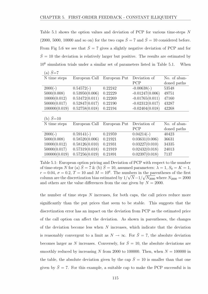
CHAPTER 5. FIRST-ORDER FEEDBACK - CONSTANT ILLIQUIDITY
Table 5.1 shows the option values and deviation of PCP for various time-steps N
(2000, 5000, 10000 and so on) for the two caps S = 7 and S = 10 considered before.
From Fig 5.6 we see that S = 7 gives a slightly negative deviation of PCP and for
S = 10 the deviation is relatively larger but positive. The results are estimated by
106 simulation trials under a similar set of parameters listed in Table 5.1. When
(a) S=7N time steps European Call European Put Deviation of No. of aban-
PCP doned paths2000(-) 0.54572(-) 0.22242 -0.00638(-) 535485000(0.008) 0.53950(0.006) 0.22229 -0.01247(0.006) 4975110000(0.012) 0.53472(0.011) 0.22269 -0.01765(0.011) 4716050000(0.017) 0.52847(0.017) 0.22190 -0.02312(0.017) 43287100000(0.019) 0.52758(0.018) 0.22194 -0.02404(0.018) 42268
(b) S=10N time steps European Call European Put Deviation of No. of aban-
PCP doned paths2000(-) 0.59141(-) 0.21959 0.04214(-) 404235000(0.008) 0.58520(0.006) 0.21921 0.03631(0.006) 3663110000(0.012) 0.58126(0.010) 0.21931 0.03227(0.010) 3433550000(0.017) 0.57319(0.018) 0.21919 0.02432(0.018) 24013100000(0.019) 0.57256(0.019) 0.21891 0.02397(0.018) 7137
Table 5.1: European option pricing and Deviation of PCP with respect to the numberof time-steps N for (a) S = 7 & (b) S = 10, assumed parameters: λ = 1, S0 = K = 1,r = 0.04, σ = 0.2, T = 10 and M = 106. The numbers in the parentheses of the firstcolumn are the discretization bias estimated by 1/
√N−1/
√N2000 whereN2000 = 2000
and others are the value differences from the one given by N = 2000.
the number of time steps N increases, for both caps, the call prices reduce more
significantly than the put prices that seem to be stable. This suggests that the
discretization error has an impact on the deviation from PCP as the estimated price
of the call option can affect the deviation. As shown in parentheses, the changes
of the deviation become less when N increases, which indicate that the deviation
is reasonably convergent to a limit as N → ∞. For S = 7, the absolute deviation
becomes larger as N increases. Conversely, for S = 10, the absolute deviations are
smoothly reduced by increasing N from 2000 to 100000. Then, when N = 100000 in
the table, the absolute deviation given by the cap S = 10 is smaller than that one
given by S = 7. For this example, a suitable cap to make the PCP successful is in
115

CHAPTER 5. FIRST-ORDER FEEDBACK - CONSTANT ILLIQUIDITY
the range between 7 and 10 subject to the number of time steps N chosen. We also
provide the number of abandoned paths with S = 7 and S = 10 in the last column of
Table 5.1. It shows that the number of abandoned paths is decreasing as N increases.
Compared with S = 7, S = 10 leads to less abandoned paths and its decrease is more
rapid than S = 7.
We previously noted that either over-capped prices or negative prices are triggered
by a nearly zero denominator, ε = 1 − λSV BSSS → 0, where ε can be positive or
negative, therefore the location (S, τ) which has the potential for over-capping prices
can be deduced by a similar analysis to that used to estimate the abandoning region
with ε∗ for negative prices (shown in Eq (5.16)). Consider a underlying price process
S(ti) generated at discrete time ti = i∆t, i = 0, · · · , N with equal time steps ∆t. If
S(tm+1) > S and S(ti) ≤ S for any i ≤ m, then the following inequalities must be
satisfied:
Zm
ε>
S/S(tm)− 1− r∆t
σ√
∆t,
Zm
ε> 0 ,
where Zm is a standard normal random variable to simulate S(tm+1). The second
inequality ensures the same signs of Zm and ε, i.e. Zm
ε= |Zm|
|ε| , then the inequalities
simply become:
|Zm||ε| >
S/S(tm)− 1− r∆t
σ√
∆t. (5.21)
We will prove that if the inequality (5.21) holds, then
ε→ 0 or S(tm) > S/(1 + r∆t) .
For any given value of S(tm) such that 0 < S(tm) < S/(1 + r∆t), (5.21) can be
written as:
|ε| < σ√
∆t|Zm|S/S(tm)− 1− r∆t
, (5.22)
which suffices to show that |ε| → 0 because the right hand of the inequality (5.22)
tends to zero as the expectation value of |Zm| → 0; otherwise, for any given value of
S(tm) such that S/(1 + r∆t) < S(tm) < S, we derive an opposite inequality:
|ε| > σ√
∆t|Zm|S/S(tm)− 1− r∆t
, (5.23)
116
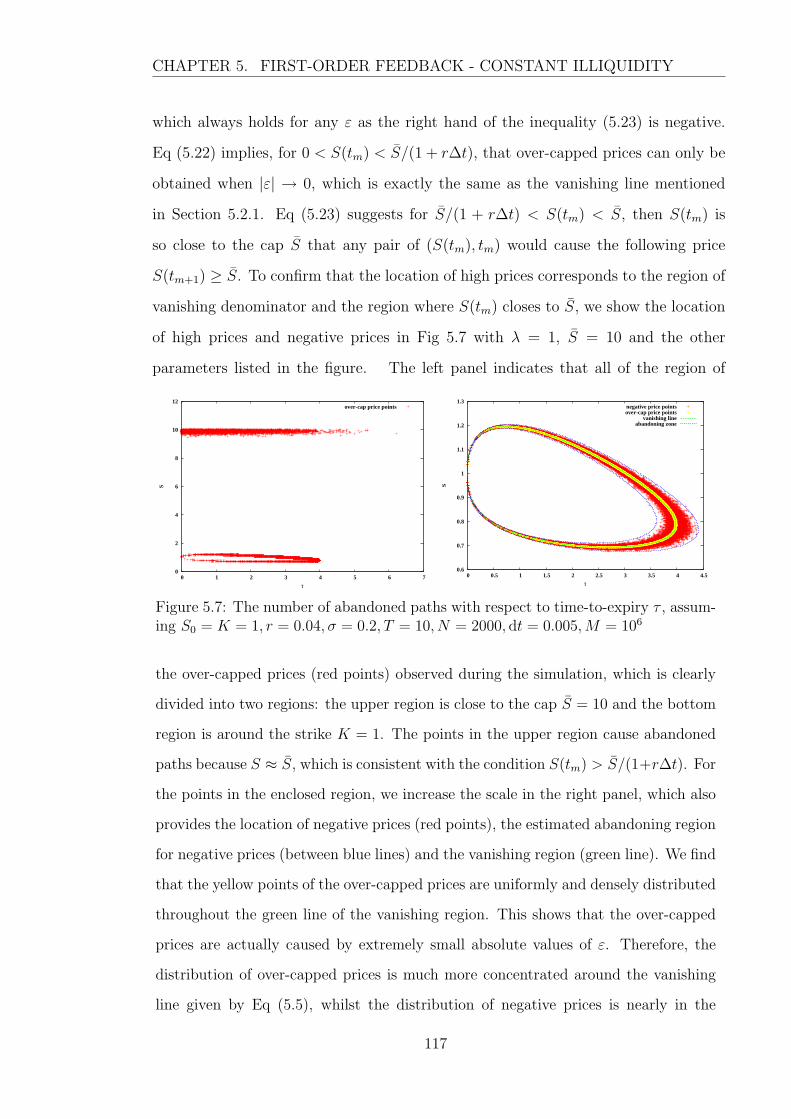
CHAPTER 5. FIRST-ORDER FEEDBACK - CONSTANT ILLIQUIDITY
which always holds for any ε as the right hand of the inequality (5.23) is negative.
Eq (5.22) implies, for 0 < S(tm) < S/(1 + r∆t), that over-capped prices can only be
obtained when |ε| → 0, which is exactly the same as the vanishing line mentioned
in Section 5.2.1. Eq (5.23) suggests for S/(1 + r∆t) < S(tm) < S, then S(tm) is
so close to the cap S that any pair of (S(tm), tm) would cause the following price
S(tm+1) ≥ S. To confirm that the location of high prices corresponds to the region of
vanishing denominator and the region where S(tm) closes to S, we show the location
of high prices and negative prices in Fig 5.7 with λ = 1, S = 10 and the other
parameters listed in the figure. The left panel indicates that all of the region of
0
2
4
6
8
10
12
0 1 2 3 4 5 6 7
S
τ
over-cap price points
0.6
0.7
0.8
0.9
1
1.1
1.2
1.3
0 0.5 1 1.5 2 2.5 3 3.5 4 4.5
S
τ
negative price pointsover-cap price points
vanishing lineabandoning zone
Figure 5.7: The number of abandoned paths with respect to time-to-expiry τ , assum-ing S0 = K = 1, r = 0.04, σ = 0.2, T = 10, N = 2000, dt = 0.005,M = 106
the over-capped prices (red points) observed during the simulation, which is clearly
divided into two regions: the upper region is close to the cap S = 10 and the bottom
region is around the strike K = 1. The points in the upper region cause abandoned
paths because S ≈ S, which is consistent with the condition S(tm) > S/(1+r∆t). For
the points in the enclosed region, we increase the scale in the right panel, which also
provides the location of negative prices (red points), the estimated abandoning region
for negative prices (between blue lines) and the vanishing region (green line). We find
that the yellow points of the over-capped prices are uniformly and densely distributed
throughout the green line of the vanishing region. This shows that the over-capped
prices are actually caused by extremely small absolute values of ε. Therefore, the
distribution of over-capped prices is much more concentrated around the vanishing
line given by Eq (5.5), whilst the distribution of negative prices is nearly in the
117

CHAPTER 5. FIRST-ORDER FEEDBACK - CONSTANT ILLIQUIDITY
entire abandoning regions. As shown in Fig 5.7, the abandoning zone covers all the
negative prices and all the over-capped prices in the lower region, which implies that
|ε| < ε∗. Moreover, in the total of 40427 abandoned paths found after simulating
106 sample paths, the number of the abandoned paths led by over-capped prices is
only 6861 whilst the number of paths with negative prices is 33566, which shows the
over-capped prices occur less frequently than the negative prices in the simulation.
5.2.3 Illiquidity λ impact on pricing option
In this subsection, we focus on how the option prices are changed by the illiquidity
λ. To be clear, we denote the volatility term, as follows:
σtot(λ) =σ
1− λSV BSSS
.
It has a hyperbolic variation with λ with a singularity at λ = 1SV BS
SS. Then the
absolute value of σtot is monotonically increasing and always larger than σ in the
region 0 ≤ λ < 1SV BS
SSand monotonically decreasing in the region λ > 1
SV BSSS
, eventually
becoming smaller than σ. It seems that the modified volatility σtot changes with
the sign of the denominator: the volatility increases in λ for positive denominators
and decreases in λ for negative denominators.3 Recall the explicit form of the zero
denominator (5.5):
S(τ) = K exp(− (r +
1
2σ2)τ ± σ
√τ√
2 log λ− log(2πσ2τ)),
subject to the restriction τ ∈ (0, τ ∗), where τ ∗ is given by (5.6):
τ ∗ =λ2
2πσ2,
which suggests that the vanishing period (0, τ ∗) increases with the square of λ (shown
in Fig 5.2). We find that negative denominators are given by those pairs (S, τ)
in the area enclosed by the curves (5.5) and the denominators remain positive for
τ ∈ (τ ∗, T ]. Due to the two opposite effects of λ on option pricing, the length of the
3The negative denominator forces the stock price changes in the opposite direction of the changeindicates by the Wiener process dW .
118

CHAPTER 5. FIRST-ORDER FEEDBACK - CONSTANT ILLIQUIDITY
period (0, τ ∗) is important in deciding which effect dominates the price process: if
the vanishing period is extended over half the maturity, we suggest that the negative
relation between option prices and λ is stronger than the positive relation, otherwise,
there is a stronger positive relation between them. Therefore, for τ ∗ = T/2, let the
particular value of λ be λ∗, which is:
λ∗ = σ√πT . (5.24)
Using the similar parameters: S0 = K = 1, r = 0.04, σ = 0.2, T = 10, N = 2000
and M = 106, then λ∗ is approximated as 1.121. There is another specific value of
λ, denoted by λ, which makes (S(τ), τ) lie in the vanishing circle when τ = T . By
Eq (5.5) with known S(τ) = K = 1 as τ = T , such λ can be expressed in an explicit
form:
λ = σ√
2πT exp((r + 1
2σ2)2T
2σ2
).
Fig 5.8 provides evidence of the impact of λ on pricing European call options in
the upper panel and European put options in the bottom panel. The Black-Scholes
prices for a perfect liquid market are also indicated by straight green lines in these
figures for comparison. We set a cap S = 10 in order to avoid those paths with
abnormally large underlying prices in this example and all the results presented in
the figures are estimated by 106 sample paths. In Fig 5.9, we also provide average
values of the volatility σtot with respect to each λ and the corresponding deviation
of PCP . From Fig 5.8, we find clear evidence that λ has two opposite effects on
option prices. Consistent with the estimator λ∗ ≈ 1.1 suggested above, we notice in
the range λ < 1.1, the option price is strictly increasing in λ, which is by implication
larger than the corresponding price given by the Black-Scholes formula. However, for
λ > 1.1, the option price is decreasing in λ in general, and eventually drops down
below the Black-Scholes price. The price changes are consistent with the volatility in
Fig 5.9(a), which shows the average volatility is increasing as λ and reaches a peak
around λ∗ = 1.1, whilst for λ > λ∗ the volatility approximately tends to decrease
with λ and would be even lower than the constant volatility value σ = 0.2 for the
Black-Scholes model when λ > 3. The reason for such a low volatility is because
119
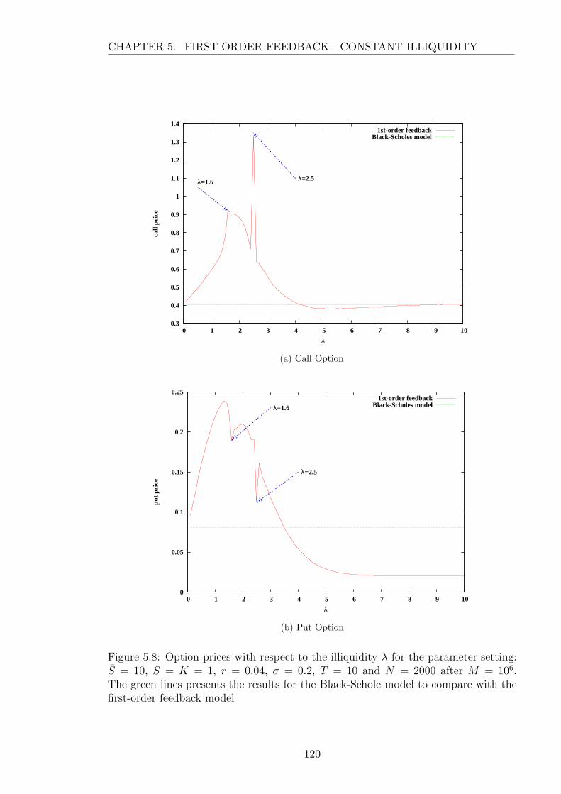
CHAPTER 5. FIRST-ORDER FEEDBACK - CONSTANT ILLIQUIDITY
0.3
0.4
0.5
0.6
0.7
0.8
0.9
1
1.1
1.2
1.3
1.4
0 1 2 3 4 5 6 7 8 9 10
call
pric
e
λ
λ=2.5λ=1.6
1st-order feedbackBlack-Scholes model
(a) Call Option
0
0.05
0.1
0.15
0.2
0.25
0 1 2 3 4 5 6 7 8 9 10
put
pric
e
λ
λ=2.5
λ=1.61st-order feedback
Black-Scholes model
(b) Put Option
Figure 5.8: Option prices with respect to the illiquidity λ for the parameter setting:S = 10, S = K = 1, r = 0.04, σ = 0.2, T = 10 and N = 2000 after M = 106.The green lines presents the results for the Black-Schole model to compare with thefirst-order feedback model
120

CHAPTER 5. FIRST-ORDER FEEDBACK - CONSTANT ILLIQUIDITY
0.05
0.1
0.15
0.2
0.25
0.3
0 1 2 3 4 5 6 7 8 9 10
aver
age
vola
tilit
y
λ
λ=1.1
λ=1.6
1st-order feedbackBlack-Scholes model
(a) Average Volatility
0
0.2
0.4
0.6
0.8
1
0 1 2 3 4 5 6 7 8 9 10
devi
atio
n of
PC
P
λ
λ=1.6
λ=2.5
1st-order feedbackBlack-Scholes model
(b) Deviation of PCP
Figure 5.9: Average volatility & deviation of PCP with respect to the illiquidity λusing the same parameter setting as the previous Fig 5.8. The green lines presentsthe results for the Black-Schole model to compare with the first-order feedback model
121

CHAPTER 5. FIRST-ORDER FEEDBACK - CONSTANT ILLIQUIDITY
the absolute value of the denominator of the volatility is larger than 1 when λ is
sufficiently large. It is clear that the case of λ > 1.1 is more complicated because
we found kinks around λ = 1.6 and λ = 2.5. At or near these kinks, the call price
jumps up while the put price just falls slightly. The biggest positive jump occurs
at λ = 2.5 which is nearly equal to the value of λ, mainly because the denominator
1−λSVss ≈ 0 at the initial time t0. Fig 5.10 reinforces this point by a comparison of
λ = 1.0 and λ = 2.5. In detail, we find the paths simulated by the first-order model
0
0.5
1
1.5
2
2.5
3
3.5
4
4.5
5
0 2 4 6 8 10
S
t
λ = 1.0
1st order feedback modelstandard model
0
0.5
1
1.5
2
2.5
3
3.5
4
0 2 4 6 8 10
S
t
λ = 2.5
1st order feedback modelstandard model
Figure 5.10: Random paths with illiquidity λ = 1.0, λ = 2.5 and λ = 0.0. The redpaths stand for 1st order feedback model and the green paths for standard Black-Scholes model (i.e. λ = 0.0). Use the same parameter setting as the previous Fig 5.8.
can fluctuate much more than the standard Black-Scholes model. For the particular
case of λ = 2.5, the underlying prices S(t1) become more volatile than the case of
λ = 1, which causes the highest abandonment rate (around 47%) when λ = 2.5. As
the restriction of the price: 0 ≤ S ≤ 10 with S(t0) = 1, there is more opportunities
for call options to earn money than put options. Furthermore, the deviation from
PCP shown in Fig 5.9(b) has a similar shape to the call prices with two significant
kinks occurring near λ = 1.6 and λ = 2.5, which implies that the deviation from
PCP is mainly determined by the estimate of the call option rather than the put
option. We also provide the impact of λ on the deviation from PCP with different
sizes of the cap: S = 5, 7 and 10 in Fig 5.11. This suggests the lower deviation
is given by the lower cap, which is consistent with the findings in Section 5.2.2, so
that using a suitable cap can ensure that the PCP is reasonably well satisfied for a
given λ. However, the idea of using a constant cap to fix all cases with different λ
122

CHAPTER 5. FIRST-ORDER FEEDBACK - CONSTANT ILLIQUIDITY
-0.4
-0.2
0
0.2
0.4
0.6
0.8
1
0 1 2 3 4 5 6 7 8 9 10
erro
r
λ
cap=5cap=7
cap=10
Figure 5.11: Error of put-call parity changes with respect to illiquidity λ in the casesof different caps S with parameters: S = K = 1, r = 0.04, σ = 0.2, T = 10 andN = 2000 after M = 105
is unrealistic. The deviation curves still have a similar shape for different caps in
Fig 5.11 with two kinks near λ = 1.6 and λ = 2.5.
To sum up, in the first-order feedback model, the option will become more expen-
sive when the market becomes more illiquid in a reasonable range λ ∈ [0, λ∗], where
there is a positive relation between λ and option prices. For λ > λ∗, the option prices
will have a negative relation with λ, consequently, it will be cheaper than in a liquid
market.
5.3 Comparison with Glover (2008) model
There is a slightly different SDE employed in Glover (2008), which is:
dS = rSdt+σS
1− λV BSSS
dW , (5.25)
where λ is some constant. The difference arises because his model only captures the
price impact of the trading volume, but we extend it to account for the price impact
of the present market value of the trading. Therefore, we apply a similar scheme
introduced in Section 5.1 to estimate option prices and check the deviation from
PCP. The parameters have been used in Glover (2008): K = 1, r = 0.04, σ = 0.2
123

CHAPTER 5. FIRST-ORDER FEEDBACK - CONSTANT ILLIQUIDITY
and T = 1 with different λ = 0, 0.09, 0.1, 1, 2, 5 and 10. The additional parameters
for our simulation are set as: S = 1, N = 2000, M = 106. It is pointed out in Glover
(2008) that there exists a vanishing denominator region, which has a similar form to
Eq (5.5), namely:
S(τ) = K exp(− (r +
3
2σ2)τ ± σ
√2τ
[(r + σ2)τ + log
( λ
σK√
2πτ
)] 12). (5.26)
Notice that for a given τ , we can gain two distinct values of S(τ) unless τ = 0 or the
following equation is satisfied:
(r + σ2)τ + log( λ
σK√
2πτ
)= 0 , (5.27)
which gives a single value of S(τ). Let τ = τ ∗ be a solution to Eq (5.27), then the
vanishing region is written as (0, τ ∗), and for τ > τ ∗, there is no chance to obtain
vanishing denominators. However, we cannot explicitly solve for τ ∗ from Eq (5.27),
which is different from our model where τ ∗ can be expressed by Eq (5.24). This
implies that a finite value of τ ∗ must be found in our model, but it might not exist in
Glover (2008) model. If there is a solution τ ∗ to Eq (5.27) and τ ∗ ∈ R, then λ must
satisfy:
λ ≤ σK√
2πτ , (5.28)
otherwise, the equation (5.27) cannot be solved, and for any τ , there always exist
two distinct values of S(τ) given by Eq (5.26). Glover (2008) studies the period of
close to maturity for relatively small λ, such as λ = 0.1 and 0.09 under the parameter
setting given above. The inequality (5.28) suggests that λ ≤ 0.50√τ . For maturity
T = 1, if we need the length of the vanishing region τ ∗ which is less than T , then
λ ≤ σK√
2πτ ≤ σK√
2πT = 0.50 . (5.29)
Fig 5.12 shows the vanishing region with respect to λ in the range 0.09 to 10 for the
Glover (2008) model and our model. We find that the region expands significantly as
λ increases. For smaller values λ = 0.09 and 0.1 that satisfy the condition (5.29), τ ∗
is shown to be around 0.03 and 0.04 respectively in the two magnified figures, which
suggests that the vanishing regions given by both models are limited and relatively
124
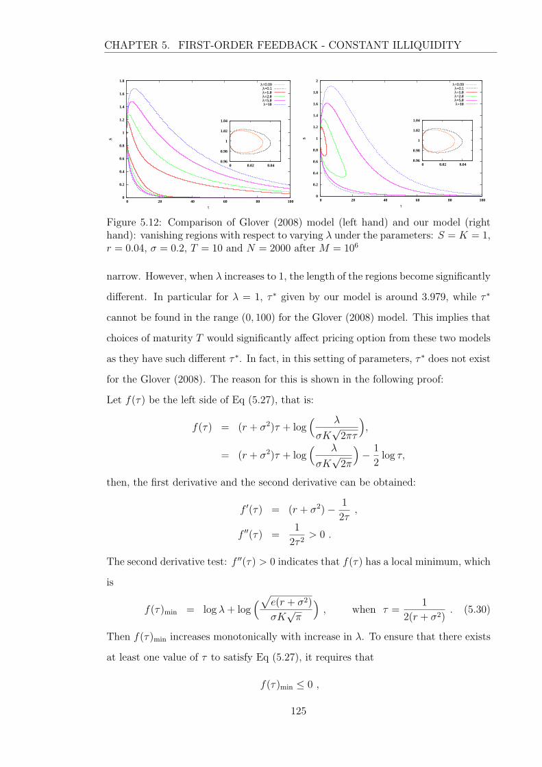
CHAPTER 5. FIRST-ORDER FEEDBACK - CONSTANT ILLIQUIDITY
0
0.2
0.4
0.6
0.8
1
1.2
1.4
1.6
1.8
0 20 40 60 80 100
S
τ
λ=0.09λ=0.1λ=1.0λ=2.0λ=5.0λ=10
0.96
0.98
1
1.02
1.04
0 0.02 0.04
0
0.2
0.4
0.6
0.8
1
1.2
1.4
1.6
1.8
2
0 20 40 60 80 100
S
τ
λ=0.09λ=0.1λ=1.0λ=2.0λ=5.0λ=10
0.96
0.98
1
1.02
1.04
0 0.02 0.04
Figure 5.12: Comparison of Glover (2008) model (left hand) and our model (righthand): vanishing regions with respect to varying λ under the parameters: S = K = 1,r = 0.04, σ = 0.2, T = 10 and N = 2000 after M = 106
narrow. However, when λ increases to 1, the length of the regions become significantly
different. In particular for λ = 1, τ ∗ given by our model is around 3.979, while τ ∗
cannot be found in the range (0, 100) for the Glover (2008) model. This implies that
choices of maturity T would significantly affect pricing option from these two models
as they have such different τ ∗. In fact, in this setting of parameters, τ ∗ does not exist
for the Glover (2008). The reason for this is shown in the following proof:
Let f(τ) be the left side of Eq (5.27), that is:
f(τ) = (r + σ2)τ + log( λ
σK√
2πτ
),
= (r + σ2)τ + log( λ
σK√
2π
)− 1
2log τ,
then, the first derivative and the second derivative can be obtained:
f ′(τ) = (r + σ2)− 1
2τ,
f ′′(τ) =1
2τ 2> 0 .
The second derivative test: f ′′(τ) > 0 indicates that f(τ) has a local minimum, which
is
f(τ)min = log λ+ log(√
e(r + σ2)
σK√π
), when τ =
1
2(r + σ2). (5.30)
Then f(τ)min increases monotonically with increase in λ. To ensure that there exists
at least one value of τ to satisfy Eq (5.27), it requires that
f(τ)min ≤ 0 ,
125

CHAPTER 5. FIRST-ORDER FEEDBACK - CONSTANT ILLIQUIDITY
which means
λ ≤ σK√π√
e(r + σ2).
Under the parameters used in Fig 5.12, the range of λ is estimated to be λ ≤ 0.760.
This is clear that λ = 1 is beyond the range, therefore, there is no solution τ (i.e. τ ∗)
to Eq (5.28) in this case.
To compare both models easily, we focus on analysing the changes of put options,
rather than call options which are more problematic due to the dependency on the
sizes of caps. In Fig 5.13, there are two different maturities T = 1 (top panels) and
0
0.02
0.04
0.06
0.08
0.1
0.12
0 100000 200000 300000 400000 500000 600000 700000 800000 900000 1e+06
put
pric
e
no. of paths
λ=0.0λ=0.09λ=0.1λ=1.0λ=2.0λ=5.0λ=10
0
0.02
0.04
0.06
0.08
0.1
0.12
0 100000 200000 300000 400000 500000 600000 700000 800000 900000 1e+06
put
pric
e
no. of paths
λ=0.0λ=0.09λ=0.1λ=1.0λ=2.0λ=5.0λ=10
(a) T = 1
0
0.05
0.1
0.15
0.2
0.25
0.3
0 100000 200000 300000 400000 500000 600000 700000 800000 900000 1e+06
put
pric
e
no. of paths
λ=0.0λ=0.09
λ=0.1λ=1.0λ=2.0λ=5.0λ=10
0
0.05
0.1
0.15
0.2
0.25
0.3
0 100000 200000 300000 400000 500000 600000 700000 800000 900000 1e+06
put
pric
e
no. of paths
λ=0.0λ=0.09
λ=0.1λ=1.0λ=2.0λ=5.0λ=10
(b) T = 10
Figure 5.13: Comparison of Glover (2008) model (left hand) and our model (righthand): put prices for T = 1 (a) and T = 10 (b) with respect to varying λ under theparameters: S = K = 1, r = 0.04, σ = 0.2, T = 10 and N = 2000 after M = 106
T = 10 (bottom panels) employed to estimate put prices. In the case of the maturity
126

CHAPTER 5. FIRST-ORDER FEEDBACK - CONSTANT ILLIQUIDITY
T = 1, both models have a similar value of τ ∗ < T for smaller values of λ (0.09 and
0.1) whilst for larger values of λ (1, 2, 5 and 10), T is clearly shorter than τ ∗ for
both models so that they have a similar impact of τ ∗. Therefore, we find that the
option prices shown in the top panels are very close to each other. Except for the
choices λ = 0.09 and 0.1, the other prices for T = 1 are lower than the corresponding
Black-Scholes prices and apparently reduced monotonically as λ increases, which is
also shown in Glover (2008). Thus, it is natural to consider that for both models
the put price first increases for relatively small λ then decreases when λ > λ∗, as
discussed in the previous section.
In the case of T = 10, the prices estimated by our model are clearly higher than
the prices given by the Glover (2008) model when λ = 1 and λ = 2, because the
maturity is long enough to show the difference of τ ∗ for two models: τ ∗ in our model
is less than 20 and much smaller than that in Glover’s model (see Fig 5.12), which
implies that the underlying in our model has more possibility of hitting the vanishing
circle. Both models produce higher put prices than Black-Scholes prices when λ < 5
because of the existence of the vanishing regions. When λ = 5 and λ = 10, the
prices become close again as the corresponding value of τ ∗ for both models are large,
which also implies that their prices are lower than the Black-Scholes price as the
vanishing regions are hard to hit. The put prices for T = 10 are still decreasing as
λ increases in results that all the values of λ here are nearly lager than λ∗. We
also give the results of call options and deviations of PCP in Fig 5.14 and show
without caps, the estimated prices of call options cannot converge by increasing the
number of paths, due to the presence of extremely high prices in the underlying.
Call options are overpriced by both models by the unexpected big jumps, and the
deviations of PCP in the bottom panel are obviously seen to be seriously affected by
the corresponding call prices. Therefore, in both models used here for pricing a call
option, we suggest estimating the associated put price and then extract the call price
from put-call parity.
127

CHAPTER 5. FIRST-ORDER FEEDBACK - CONSTANT ILLIQUIDITY
0
0.5
1
1.5
2
2.5
3
3.5
4
0 100000 200000 300000 400000 500000 600000 700000 800000 900000 1e+06
call
pric
e
no. of paths
λ=0.0λ=0.09λ=0.1λ=1.0λ=2.0λ=5.0λ=10
0
0.5
1
1.5
2
2.5
3
3.5
4
0 100000 200000 300000 400000 500000 600000 700000 800000 900000 1e+06
call
pric
e
no. of paths
λ=0.0λ=0.09λ=0.1λ=1.0λ=2.0λ=5.0λ=10
(a) call price
-0.5
0
0.5
1
1.5
2
2.5
3
3.5
0 100000 200000 300000 400000 500000 600000 700000 800000 900000 1e+06
devi
atio
n of
PC
P
no. of paths
λ=0.0λ=0.09
λ=0.1λ=1.0λ=2.0λ=5.0λ=10
-0.5
0
0.5
1
1.5
2
2.5
3
3.5
0 100000 200000 300000 400000 500000 600000 700000 800000 900000 1e+06
devi
atio
n of
PC
P
no. of paths
λ=0.0λ=0.09
λ=0.1λ=1.0λ=2.0λ=5.0λ=10
(b) deviation of PCP
Figure 5.14: Comparison of Glover (2008) model (left hand) and our model (righthand): call prices (a) and deviation of PCP (b) with respect to varying λ under theparameters: S = K = 1, r = 0.04, σ = 0.2, T = 10 and N = 2000 after M = 106
128
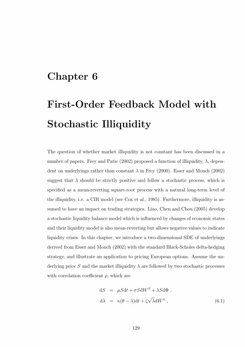
Chapter 6
First-Order Feedback Model with
Stochastic Illiquidity
The question of whether market illiquidity is not constant has been discussed in a
number of papers. Frey and Patie (2002) proposed a function of illiquidity, λ, depen-
dent on underlyings rather than constant λ in Frey (2000). Esser and Monch (2002)
suggest that λ should be strictly positive and follow a stochastic process, which is
specified as a mean-reverting square-root process with a natural long-term level of
the illiquidity, i.e. a CIR model (see Cox et al., 1985). Furthermore, illiquidity is as-
sumed to have an impact on trading strategies. Liao, Chen and Chou (2005) develop
a stochastic liquidity balance model which is influenced by changes of economic states
and their liquidity model is also mean-reverting but allows negative values to indicate
liquidity crises. In this chapter, we introduce a two-dimensional SDE of underlyings
derived from Esser and Monch (2002) with the standard Black-Scholes delta-hedging
strategy, and illustrate an application to pricing European options. Assume the un-
derlying price S and the market illiquidity λ are followed by two stochastic processes
with correlation coefficient ρ, which are
dS = µSdt+ σSdW S + λSdΦ ,
dλ = κ(θ − λ)dt+ ζ√λdW λ , (6.1)
129

CHAPTER 6. FIRST-ORDER FEEDBACK - STOCHASTIC ILLIQUIDITY
where µ and σ denote the constant drift and volatility for the underlying S; Φ is the
number of shares traded by large investors; λ follows a one-factor CIR model which
ensures the mean-reversion of illiquidity λ towards the long-run value θ with speed of
adjustment κ and the volatility of this process ζ. dW S and dW λ are two correlated
Brownian motions with correlation coefficient ρ as follows:
dW SdW λ = ρdt .
The ρ could be positive or negative, whose effects on option pricing will be addressed
in Section 6.2.2. Using Cholesky decomposition, Eq (6.1) can be rewritten with two
uncorrelated standard Brownian motions W and W
dS = µSdt+ σSdW + λSdΦ ,
dλ = κ(θ − λ)dt+ ρζ√λdW +
√1− ρ2ζ
√λdW . (6.2)
To present a complete derivation, we assume the illiquidity λ has an impact on the
number of shares Φ(t, S, λ) held by large investors, then by applying Ito’s lemma to
the function of Φ(t, S, λ), we should find
dΦ = Φtdt+ ΦSdS + Φλdλ
+1
2(ΦSSdS2 + Φλλdλ
2 + 2ΦλSdλdS)
= Φtdt+ ΦSdS + Φλdλ+1
2Φλλζ
2λdt
+1
2ΦSSdS2 + ΦλSdλdS ,
where the subscripts are used to denote partial derivatives. Substituting this into
Eq (6.2) leads to
(1− λSΦS)dS = (µ
λ+ Φt + κ(θ − λ)Φλ +
1
2Φλλζ
2λ)λSdt
+(σ + λΦλρζ√λ)SdW
+λΦλ
√1− ρ2ζ
√λSdW
+1
2λSΦSSdS2 + λSΦλSdλdS . (6.3)
Assuming the SDE of S has the general form:
dS = b(t, S, λ)dt+ v(t, S, λ)SdW + v(t, S, λ)SdW , (6.4)
130

CHAPTER 6. FIRST-ORDER FEEDBACK - STOCHASTIC ILLIQUIDITY
which implies, as dt→ 0,
dS2 = (v2 + v2)S2dt ,
dλdS = (ρv +√
1− ρ2v)ζ√λSdt .
Comparing the coefficients of each term, v, v and b can be obtained from
v(t, S, λ) =σ
1− λSΦS
+ ρλΦλζ
√λ
1− λSΦS
, (6.5)
v(t, S, λ) =√
1− ρ2λΦλζ
√λ
1− λSΦS
, (6.6)
b(t, S, λ) =λS
1− λSΦS
[µλ
+ Φt + κ(θ − λ)Φλ +1
2Φλλζ
2λ
+1
2ΦSSS
2(v2 + v2) + ζ√λΦλSS(ρv +
√1− ρ2v)
]. (6.7)
Therefore, the dynamics of S and λ are given by
dS = b(t, S, λ)dt+ v(t, S, λ)SdW + v(t, S, λ)SdW , (6.8)
dλ = κ(θ − λ)dt+ ρζ√λdW +
√1− ρ2ζ
√λdW , (6.9)
where v(t, S, λ), v(t, S, λ) and b(t, S, λ) are prescribed in Eq (6.5)-(6.7). Moreover, in
the risk-neutral world, we deduce the SDEs with a drift adjustment as
dS = rSdt+( σ
1− λSΦS
+ ρλΦλζ
√λ
1− λSΦS
)SdW
+√
1− ρ2λΦλζ
√λ
1− λSΦS
SdW , (6.10)
dλ = κ(θ − λ)dt+ ρζ√λdW +
√1− ρ2ζ
√λdW . (6.11)
Again, price takers in the first-order feedback model are assumed to use a sub-optimal
delta hedging according to the standard Black-Scholes formula, i.e. ΦS = V BSSS . For
simplicity, we consider the function of Φ is independent of the illiquidity λ i.e. Φλ = 0,
where the liquidity has no impact on the strategy of the larger trader. This leads to
a simple form of equation system for the first-order feedback models, as follows:
dS = rSdt+σS
1− λSV BSSS
dW , (6.12)
dλ = κ(θ − λ)dt+ ρζ√λdW +
√1− ρ2ζ
√λdW . (6.13)
Naturally, for the full feedback model, V BSSS is replaced by VSS.
131

CHAPTER 6. FIRST-ORDER FEEDBACK - STOCHASTIC ILLIQUIDITY
The remainder of the chapter is organized as follows: Section 6.1 briefly intro-
duces the implementation of the first-order feedback model with stochastic illiquidity
and Section 6.2 presents a detailed analysis with respect to the denominator of the
volatility term and option pricing in the stochastic illiquidity model is compared with
the constant illiquidity case.
6.1 Implementation
We apply a Monte Carlo scheme to implement pricing of the two-dimensional problem,
i.e. the first-order feedback with stochastic illiquidity λ(t) as detailed in Eq (6.12)-
(6.13). The algorithm used here is quite similar to that applied in Section 5.1 for
simulating the underlying S(t), but with varying λ(t) at time points t1, · · · , tN which
are also estimated by a simple Euler discretization of Eq (6.13). For a European call
option price V (t), a detailed implementation is given as follows:
1. Set N discrete time points ti for i = 0, · · · , N in time interval [0, T ] with the
same increment, i.e. ti+1 = ti + ∆t for the sake of easy implementation.
2. Generate M sample paths Sj(ti) for j = 1, · · · ,M by a simple Euler discretiza-
tion. As dW is an increment of Brownian motion W , by the basic property
of Brownian motion we can gain its estimate: Z√
∆t with a standard normal
random variable Z ∼ N(0, 1). Then the approximation of Eq (6.12) can be
obtained as follows:
Sj(ti+1) = Sj(ti) + rSj(ti)∆t+σSj(ti)
1− λj(ti)Sj(ti)V BSSSj
(ti)Zj(ti)
√∆t ,
where the second differential V BSSSj
(ti) is directly given by the Black-Scholes for-
mula for Gamma, given in Eq (5.3). Notice there is the same serious problem
as in the constant illiquidity model: the possibility of nearly vanishing denom-
inators of the volatility term would cause either negative prices or abnormally
high prices. As the illiquidity λ is now variable, the problem seems to be more
complicated. As before, we discard those paths with negative prices or above-
cap prices and set the relative option prices Vj(t0) = 0. The total number of
132

CHAPTER 6. FIRST-ORDER FEEDBACK - STOCHASTIC ILLIQUIDITY
abandoned paths is stored as m.
3. Simulate the corresponding value of λj(ti) at each time point ti for each path
Sj based on the square-root diffusion shown in Eq (6.13), as follows:
λj(ti+1) = λj(ti) + κ(θ − λj(ti))∆t+ ρζ√λj(ti)Zj(ti)
√∆t
+√
1− ρ2ζ√λj(ti)Zj(ti)
√∆t , (6.14)
where Zj(ti) is a standard normal random number and independent of Zj(ti).
As discussed in Section 3.5 for modelling stochastic volatility in jump diffusion
processes, the continuous-time CIR model is able to prevent λ from negative
values with a suitable parameter setting which does not work for a discrete-
time version. Thus, similar to the measure taken to deal with the occurrence
of negative values of volatility in Section 3.5.1, if λj(ti+1) < 0 in the jth path,
we resimulate the sample paths for λj(ti) and Sj(ti) from t1 to tN .
4. Calculate the option payment at maturity Vj(tN) = (Sj(tN) −K, 0)+ and dis-
count it back to initial time t0 by the discount factor e−rT to get the price of
option Vj(t0) for each paths Sj.
5. Then the expected option price is estimated as the averaged value of option
prices Vj(t0), i.e.
V (t0) =1
M −m
M∑j=1
Vj(t0) ,
where m is the number of discarded paths during the procedure. Then, the
law of large numbers ensures that the estimator V (t0) converges to the exact
expected value V (t0).
6.2 Comparison between constant and stochastic
illiquidity parameter
Esser and Monch (2002) suggest that the stochastic λ model shown (6.12)-(6.13)
should have little difference with the corresponding constant λmodel due to excluding
133

CHAPTER 6. FIRST-ORDER FEEDBACK - STOCHASTIC ILLIQUIDITY
the impact of λ on the trading strategy, i.e. setting Φλ = 0. However, we do obtain
some differences between the two models from our numerical results. In the remainder
of this section, we discuss the difference between the two models in two ways: the
changes of the denominator of the volatility term, which includes an analysis of
abandoning paths and put-call parity; and an impact of the choice of parameters on
option pricing.
6.2.1 Denominator of the volatility term
As with the constant illiquidity model, there is also a possibility of finding vanishing
denominators from the stochastic illiquidity model. To make the results from these
two models comparable, we assume the same default parameters1 for both models:
S0 = K = 1, r = 0.04, σ = 0.2, T = 10, N = 2000, M = 106, κ = 0.35, ζ = 0.2
and θ = 1; the stochastic illiquidity λ starts from λ0 = 1 and the constant illiquidity
λc = 1; the correlation between the underlying process and its illiquidity is considered
to be zero, i.e. ρ = 0. Unless otherwise stated, these parameters will be applied
throughout this section.
1. Negative Prices of Underlyings
As described in Chapter 5, the first-order constant illiquidity model has a van-
ishing zone to cause abnormal price moves, which is given by (5.5):
S(τ) = K exp(− (r +
1
2σ2)τ ± σ
√τ√
2logλ− log(2πσ2τ)),
and the corresponding abandoning region for negative prices has be found by
(5.10)-(5.11). The scales of the vanishing zone (0, τ ∗) and abandoning region
(0, τ ∗out) are totally independent of the option’s maturity T and they are only
dependent on the critical value of time-to-expiry τ ∗ = λ2
2πσ2 and τ ∗out = λ2
2πσ2(1−ε)2
respectively; λ here is assumed to be constant. However, when λ follows a
stochastic process the duration will be extended to the whole option life T .
Fig 6.1 is used to illustrate this point using three examples with T = 1 (a),
1The parameters for stochastic illiquidity are taken from Esser and Monch (2002).
134

CHAPTER 6. FIRST-ORDER FEEDBACK - STOCHASTIC ILLIQUIDITY
0
100
200
300
400
500
600
700
800
900
1000
0 0.2 0.4 0.6 0.8 1
cum
ulat
ive
num
ber
of a
band
oned
pat
hs
time to maturity τ
constant illiquidity modelstochastic illiquidity model
0.7
0.8
0.9
1
1.1
1.2
1.3
0 0.1 0.2 0.3 0.4 0.5 0.6 0.7 0.8 0.9 1
S
time to maturity τ
stochastic illiquidity modelconstant illiquidity model
(a) T = 1
0
500
1000
1500
2000
2500
0 1 2 3 4 5
cum
ulat
ive
num
ber
of a
band
oned
pat
hs
time to maturity τ
constant illiquidity modelstochastic illiquidity model
0.5
0.6
0.7
0.8
0.9
1
1.1
1.2
1.3
1.4
0 0.5 1 1.5 2 2.5 3 3.5 4 4.5 5
S
time to maturity τ
stochastic illiquidity modelconstant illiquidity model
(b) T = 5
0
200
400
600
800
1000
1200
1400
1600
0 2 4 6 8 10
cum
ulat
ive
num
ber
of a
band
oned
pat
hs
time to maturity τ
constant illiquidity modelstochastic illiquidity model
0.4
0.6
0.8
1
1.2
1.4
0 1 2 3 4 5 6 7 8 9 10
S
time to maturity τ
stochastic illiquidity modelconstant illiquidity model
(c) T = 10
Figure 6.1: The cumulative number of abandoned paths caused by negative pricewith respect to time-to-expiry τ & the corresponding location of negative prices.The results are given by 106 simulated paths
135

CHAPTER 6. FIRST-ORDER FEEDBACK - STOCHASTIC ILLIQUIDITY
5 (b) and 10 (c). We provide histograms of the distribution of the number of
abandoned paths and scatter plots of the location (τ, S) leading to negative
prices. For the case with constant illiquidity λc = 1, the estimators of τ ∗
and τ ∗out are 3.98 and 4.41 respectively. Therefore, the example aims to show
the abandoning region for negative prices in pricing options with a short-term
maturity T = 1, a medium-term maturity T = 5 and a long-term maturity
T = 10 in two models2. Fig 6.1(a) with T = 1 < τ ∗ indicates both models
have the same time period of finding negative prices as the maturity T , but
the stochastic illiquidity model has a somewhat wider abandoning zone than
the constant illiquidity model. The distributions of the cumulative number
of abandoned paths seem to be similar and the total number of abandoned
paths in the stochastic illiquidity is only slightly higher than that with constant
illiquidity, as seen in Table 6.1. As shown in Fig 6.1(b), when T = 5, the
Maturity T Constant Illiquidity Stochastic Illiquidity1 18146 196785 65640 8172110 33315 51624
Table 6.1: The number of abandoned paths with negative prices in 106 sample paths.
abandoning zone of the stochastic illiquidity in the scatter plot is somewhat
wider than the constant illiquidity. Moreover, the abandoning range τ ∈ (0, τ ∗out)
is only satisfied by the constant illiquidity model, rather than the the stochastic
illiquidity whose range is still τ ∈ (0, T ). The number of abandoned paths
presented in the histogram shows there is a strong peak around t = T − τ ∗
for the constant illiquidity model, while the stochastic illiquidity model has
a moderate peak at earlier times t ≈ 0. When the maturity increases again
in Fig 6.1(c), the constant illiquidity model retains the same shape for the
abandoning zone and the distribution of the number of abandoned paths as the
case of T = 5. However, in the stochastic illiquidity model, we find an extended
abandoning zone for all τ ∈ (0, T ) with T = 10, and the maximum cumulative
2Notice that T = 5 is close to 4.41 for τ∗out calculated in the constant illiquidity model.
136

CHAPTER 6. FIRST-ORDER FEEDBACK - STOCHASTIC ILLIQUIDITY
number of negative paths occurs at the critical time t = T − τ ∗.
The main results from Fig 6.1 reveal that negative prices are found during the
entire life in the stochastic illiquidity model, whereas they are only obtained
when τ ∈ (0, τ ∗out) in the constant illiquidity model. For each level of matu-
rity, the abandoning zone of the stochastic illiquidity model is shown to be
wider than for the constant illiquidity case. Thereby, the stochastic illiquidity
model generally produces many more negative prices than the constant illiq-
uidity model, as shown in Table 6.1. In the case of T ≤ τ ∗out, the stochastic
illiquidity model still generates more abandoned paths but the difference in the
number of abandoned paths between the two models is relatively small. Both
models obtain the maximum number of negative prices when T ≈ τ ∗.
We are also interested in values of λ when negative prices occur in the stochastic
illiquidity model. Fig 6.2 gives the relative location (τ, λ) when the underlying
0
0.5
1
1.5
2
2.5
3
0 1 2 3 4 5 6 7 8 9 10
λ
time to maturity τ
T=10T=5T=1
boundary line
Figure 6.2: The location of λ for negative prices with varying maturity T . Thescattered points is given by the results of M = 106 runs.
prices S(τ) < 0 with the same parameters used in Fig 6.1. The scatter plot
shows a clear boundary line to divide the plane into two regions: the data above
the boundary line could result in negative prices otherwise the data below the
boundary should never produce negative prices. The economic implication of
137

CHAPTER 6. FIRST-ORDER FEEDBACK - STOCHASTIC ILLIQUIDITY
the results is that there exists an arbitrage opportunity when the point (τ, λ)
is above the boundary line. This is because negative prices cause arbitrage
opportunities. The boundary can be explained as follows.
As mentioned, negative prices are caused by a nearly vanishing denominator,
|1− λSV BSSS | < ε, whose solution is given by (5.8)-(5.13). However, the expres-
sions (5.10)-(5.13) become invalid once
λ <√
2πσ2τ(1− ε)2 .
Therefore, those pairs (τ, λ) that satisfy the inequality would not cause negative
prices, which implies the boundary line is given by
λ =√
2πσ2τ(1− ε)2 .
In Fig 6.2 the boundary line estimated by ε = 0.05 is shown to confirm this.
2. Put-Call Parity
Under the stochastic volatility assumption, put-call parity remains valid in the
illiquid market. This can be illustrated by a PDE approach, as follows:
As discussed in the beginning of this chapter, the risk-adjusted process are
given by Eq (6.12) and (6.13). Applying Ito’s lemma, we can find the change
of derivative’s price V (S, λ, t) is:
dV (S, λ, t) =
[σ2S2
2(1− λSV BSSS )2
∂2V
∂S2+
ρσζ√λS
1− λSV BSSS
∂2V
∂S∂λ+ζ2λ
2
∂2V
∂λ2
+rS∂V
∂S+ κ(θ − λ)
∂V
∂λ+∂V
∂t
]dt
+
[σS
1− λSV BSSS
∂V
∂S+ ρζ
√λ∂V
∂λ
]dW
+
[√1− ρ2ζ
√λ∂V
∂λ
]dW , (6.15)
given by two independent Brownian motion W and W . By analogy with Glover
(2008) using standard hedging arguments, we construct a portfolio including
one underlying asset and two call options with different maturities3. Following
3This is because there is no underlying asset with which to hedge for the illiquidity risk. Weneed two options to eliminate two sources of uncertainty dW and dW .
138

CHAPTER 6. FIRST-ORDER FEEDBACK - STOCHASTIC ILLIQUIDITY
the standard arbitrage arguments,the derivative price V (S, λ, t) with two state
variables must obey the following PDE:
σ2S2
2(1− λSV BSSS )2
∂2V
∂S2+
ρσζ√λS
1− λSV BSSS
∂2V
∂S∂λ+ζ2λ
2
∂2V
∂λ2+ rS
∂V
∂S
+(κ(θ − λ)− f(S, λ, t))∂V
∂λ+∂V
∂t− rV = 0 , (6.16)
where the unspecified term f(S, λ, t) represents the market price of the illiquid-
ity risk as the illiquidity itself cannot be traded. Define a European call option
V C(S, λ, t) and put option V P (S, λ, t). As V P (S, λ, t) satisfies the above PDE,
we can substitute the put-call parity formula:
V P (S, λ, t) = V C(S, λ, t)− S +Ke−r(T−t)
into the PDE, then we can obtain:
σ2S2
2(1− λSV BSSS )2
∂2V C
∂S2+
ρσζ√λS
1− λSV BSSS
∂2V C
∂Sλ+ζ2λ
2
∂2V C
∂λ2+ rS
∂V C
∂S
+(κ(θ − λ)− f(S, λ, t))∂V C
∂λ+∂V C
∂t− rV C = 0 ,
which is true as the call option V C(S, λ, t) also satisfies the modified Black-
Scholes equation (6.16). This suggests that a European option can be replicated
by the portfolio: V C − S + Ke−r(T−t) which has the same payoff as the put
option at maturity. The solution to the Black-Scholes PDE shows that put-
call parity still holds. However, as mentioned in the constant illiquidity case,
the problem with put-call parity still exists in the crude simulation model with
a stochastic illiquidity, in that the model is seen to produce abnormally high
underlying prices. Fig 6.3 shows evidence that for both models there are some
unexpectedly high underlying prices that disrupt the convergence in pricing a
call option, when the number of sample paths is increasing and these lead to
deviations in put-call parity by both models. The stochastic illiquidity model
appears to overprice the call options more than the constant illiquidity model.
We can find an improved value of a call option by two methods. One approach
has been introduced in the constant illiquidity model, which is to set a cap S
139
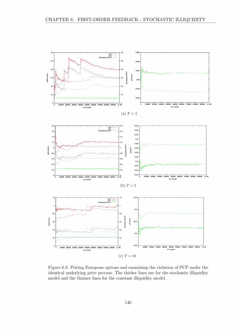
CHAPTER 6. FIRST-ORDER FEEDBACK - STOCHASTIC ILLIQUIDITY
0
0.1
0.2
0.3
0.4
0.5
0.6
0 100000 200000 300000 400000 500000 600000 700000 800000 900000 1e+06 0
0.1
0.2
0.3
0.4
0.5
0.6
opti
on p
rice
devi
atio
n of
PC
P
no. of path
CallPut
Deviation of PCP
0.056
0.058
0.06
0.062
0.064
0.066
0 100000 200000 300000 400000 500000 600000 700000 800000 900000 1e+06
put
pric
e
no. of path
(a) T = 1
0
0.2
0.4
0.6
0.8
1
1.2
1.4
1.6
1.8
0 100000 200000 300000 400000 500000 600000 700000 800000 900000 1e+06 0
0.2
0.4
0.6
0.8
1
1.2
1.4
1.6
1.8
opti
on p
rice
devi
atio
n of
PC
P
no. of path
CallPut
Deviation of PCP
0.234
0.236
0.238
0.24
0.242
0.244
0.246
0.248
0.25
0.252
0.254
0.256
0 100000 200000 300000 400000 500000 600000 700000 800000 900000 1e+06
put
pric
e
no. of path
(b) T = 5
0
0.2
0.4
0.6
0.8
1
1.2
0 100000 200000 300000 400000 500000 600000 700000 800000 900000 1e+06 0
0.2
0.4
0.6
0.8
1
1.2
opti
on p
rice
devi
atio
n of
PC
P
no. of path
CallPut
Deviation of PCP
0.205
0.21
0.215
0.22
0.225
0 100000 200000 300000 400000 500000 600000 700000 800000 900000 1e+06
put
pric
e
no. of path
(c) T = 10
Figure 6.3: Pricing European options and examining the violation of PCP under theidentical underlying price process. The thicker lines are for the stochastic illiquiditymodel and the thinner lines for the constant illiquidity model.
140

CHAPTER 6. FIRST-ORDER FEEDBACK - STOCHASTIC ILLIQUIDITY
such that we restrict S < S. The chosen value of the cap S should ensure the
smallest absolute deviation from the put-call parity. Another approach is to
estimate the value of the call option via pricing the corresponding put option.
Because put-call parity is shown to hold and the estimated price of the put
option tends to be more convergent and reliable with an increasing number of
the sample paths, as seen in the right panel of Fig 6.3, in the remainder of this
chapter we will focus on pricing put options. Then the implied call prices can
be computed by put-call parity with these known put prices.
6.2.2 Sensitivity of option price to the choice of parameters
In this section, we discuss the impact of the parameters applied in a stochastic illiq-
uidity model on option pricing, which includes maturity T , moneyness S/K, cor-
relation coefficient ρ between two dynamic processes, the adjustment speed κ and
the volatility ζ for illiquidity. Again, the remaining parameters are set as follows:
S0 = K = 1, r = 0.04, σ = 0.2 and N = 2000. Assuming the constant illiquidity
value λc = 1, then for the stochastic illiquidity we let the illiquidity start from λ0
and denote the long-term illiquidity θ with the same value as the constant illiquidity
λc, i.e. λ0 = θ = λc = 1. We will focus on European put options in the remaining
section.
1. T Impact on Option Price
A European put option price varies with the maturity T : the price generally
increases in time to maturity for a relatively short-term maturity T , but de-
creases in time to maturity for a long-term maturity, such as greater than 10
years, as seen in Fig 6.4. The figure presents the results of three models:
constant λ, stochastic λ and λ = 0. A peak of the option price appears when
T = 5: when T < 5 the option price is increasing as T rises; then for T ≥ 5
the option prices is slightly decreasing as T rises. We notice that there is a
decline in the put price for the constant illiquidity model when T = 4 because
the maturity is close to the length of the vanishing region τ ∗ which has been
141
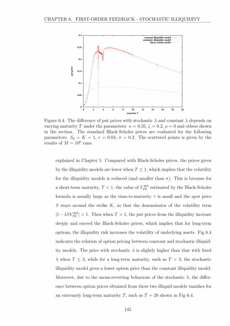
CHAPTER 6. FIRST-ORDER FEEDBACK - STOCHASTIC ILLIQUIDITY
0
0.05
0.1
0.15
0.2
0.25
0.3
0 2 4 6 8 10 12 14 16 18 20
put
pric
e
maturity T
constant illiquidity modelstochastic illiquidity model
black-scholes model
Figure 6.4: The difference of put prices with stochastic λ and constant λ depends onvarying maturity T under the parameters: κ = 0.35, ζ = 0.2, ρ = 0 and others shownin the section. The standard Black-Scholes prices are evaluated for the followingparameters: S0 = K = 1, r = 0.04, σ = 0.2. The scattered points is given by theresults of M = 106 runs.
explained in Chapter 5. Compared with Black-Scholes prices, the prices given
by the illiquidity models are lower when T ≤ 1, which implies that the volatility
for the illiquidity models is reduced (and smaller than σ). This is because for
a short-term maturity, T < 1, the value of V BSSS estimated by the Black-Scholes
formula is usually large as the time-to-maturity τ is small and the spot price
S stays around the strike K, so that the denominator of the volatility term
|1−λSV BSSS | > 1. Then when T > 1, the put prices from the illiquidity increase
deeply and exceed the Black-Scholes prices, which implies that for long-term
options, the illiquidity risk increases the volatility of underlying assets. Fig 6.4
indicates the relation of option pricing between constant and stochastic illiquid-
ity models. The price with stochastic λ is slightly higher than that with fixed
λ when T ≤ 3, while for a long-term maturity, such as T > 3, the stochastic
illiquidity model gives a lower option price than the constant illiquidity model.
Moreover, due to the mean-reverting behaviour of the stochastic λ, the differ-
ence between option prices obtained from these two illiquid models vanishes for
an extremely long-term maturity T , such as T = 20 shown in Fig 6.4.
142

CHAPTER 6. FIRST-ORDER FEEDBACK - STOCHASTIC ILLIQUIDITY
2. Moneyness S/K Impact on Option Price
The example shown in Fig 6.5 highlights the impact of moneyness on put option
prices, with particular parameters below the figure. The left panel compares
0
0.1
0.2
0.3
0.4
0.5
0.6
0.7
0.8
0.9
0 0.2 0.4 0.6 0.8 1 1.2 1.4 1.6 1.8 2
put
pric
e
moneyness S/K
PconstPstoch
Pblack-scholes
0.15
0.2
0.25
0.3
0.35
0.4
0.45
0.5
0.55
0.6
0.65
0 0.2 0.4 0.6 0.8 1 1.2 1.4 1.6 1.8 2
impl
ied
vola
tilit
y
moneyness S/K
const illiquidity modelstochastic illiquidity model
Black-Scholes model
Figure 6.5: Put prices with stochastic λ and constant λ depends on varying moneynessunder the parameters: K = 1, T = 1, κ = 0.35, ζ = 0.2, ρ = 0 and others shown inthe section. The scattered points is given by the results of M = 106 runs
the put prices produced by the three models: constant illiquidity, stochastic
illiquidity and standard Black-Scholes models using varying moneyness (S/K).
We find that the two illiquidity models give similar prices for put options with
respect to various moneyness. Compared with the Black-Scholes prices, both
models generally produce higher prices except the range: 0.9 < S/K < 1. In the
range of 0.7 < S/K < 0.9 and 1 < S/K < 1.6, the illiquidity models produce
option prices which clearly exceed the standard Black-Scholes prices and the
deviations from the Black-Scholes prices are more pronounced in the range
1 < S/K < 1.6 than those in the range 0.7 < S/K < 0.9. This implies that an
OTM option has more chance to produce a profit at expiry than an option that is
in the money when its underlying is illiquid. However, both option prices given
by the illiquidity models are close to the Black-Scholes price when the option is
deep in (S/K ¿ 0.7) or deep out of the money (S/K À 1.6). The analysis of
the deviations from the Black-Scholes prices suggest that the illiquidity model
can generate a smile and skew pattern implied volatility using the Black-Scholes
formula. From the right panel of Fig 6.5, in general, the implied volatility is
shown to be higher than the constant volatility of the Black-Scholes model. In
143
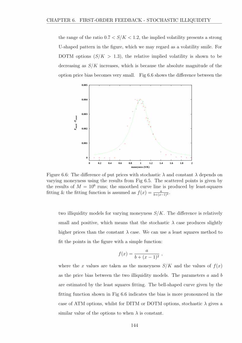
CHAPTER 6. FIRST-ORDER FEEDBACK - STOCHASTIC ILLIQUIDITY
the range of the ratio 0.7 < S/K < 1.2, the implied volatility presents a strong
U-shaped pattern in the figure, which we may regard as a volatility smile. For
DOTM options (S/K > 1.3), the relative implied volatility is shown to be
decreasing as S/K increases, which is because the absolute magnitude of the
option price bias becomes very small. Fig 6.6 shows the difference between the
0
0.001
0.002
0.003
0.004
0.005
0 0.2 0.4 0.6 0.8 1 1.2 1.4 1.6 1.8 2
Pst
och
- P
cons
t
moneyness (S/K)
Figure 6.6: The difference of put prices with stochastic λ and constant λ depends onvarying moneyness using the results from Fig 6.5. The scattered points is given bythe results of M = 106 runs; the smoothed curve line is produced by least-squaresfitting & the fitting function is assumed as f(x) = a
b+(x−1)2.
two illiquidity models for varying moneyness S/K. The difference is relatively
small and positive, which means that the stochastic λ case produces slightly
higher prices than the constant λ case. We can use a least squares method to
fit the points in the figure with a simple function:
f(x) =a
b+ (x− 1)2,
where the x values are taken as the moneyness S/K and the values of f(x)
as the price bias between the two illiquidity models. The parameters a and b
are estimated by the least squares fitting. The bell-shaped curve given by the
fitting function shown in Fig 6.6 indicates the bias is more pronounced in the
case of ATM options, whilst for DITM or DOTM options, stochastic λ gives a
similar value of the options to when λ is constant.
144
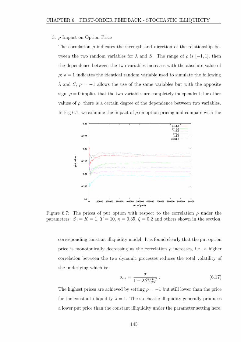
CHAPTER 6. FIRST-ORDER FEEDBACK - STOCHASTIC ILLIQUIDITY
3. ρ Impact on Option Price
The correlation ρ indicates the strength and direction of the relationship be-
tween the two random variables for λ and S. The range of ρ is [−1, 1], then
the dependence between the two variables increases with the absolute value of
ρ; ρ = 1 indicates the identical random variable used to simulate the following
λ and S; ρ = −1 allows the use of the same variables but with the opposite
sign; ρ = 0 implies that the two variables are completely independent; for other
values of ρ, there is a certain degree of the dependence between two variables.
In Fig 6.7, we examine the impact of ρ on option pricing and compare with the
0.2
0.205
0.21
0.215
0.22
0.225
0.23
0 100000 200000 300000 400000 500000 600000 700000 800000 900000 1e+06
put
pric
es
no. of paths
ρ=-1.0ρ=-0.5ρ=0.0ρ=0.5ρ=1.0
const λ
Figure 6.7: The prices of put option with respect to the correlation ρ under theparameters: S0 = K = 1, T = 10, κ = 0.35, ζ = 0.2 and others shown in the section.
corresponding constant illiquidity model. It is found clearly that the put option
price is monotonically decreasing as the correlation ρ increases, i.e. a higher
correlation between the two dynamic processes reduces the total volatility of
the underlying which is:
σtot =σ
1− λSV BSSS
. (6.17)
The highest prices are achieved by setting ρ = −1 but still lower than the price
for the constant illiquidity λ = 1. The stochastic illiquidity generally produces
a lower put price than the constant illiquidity under the parameter setting here.
145
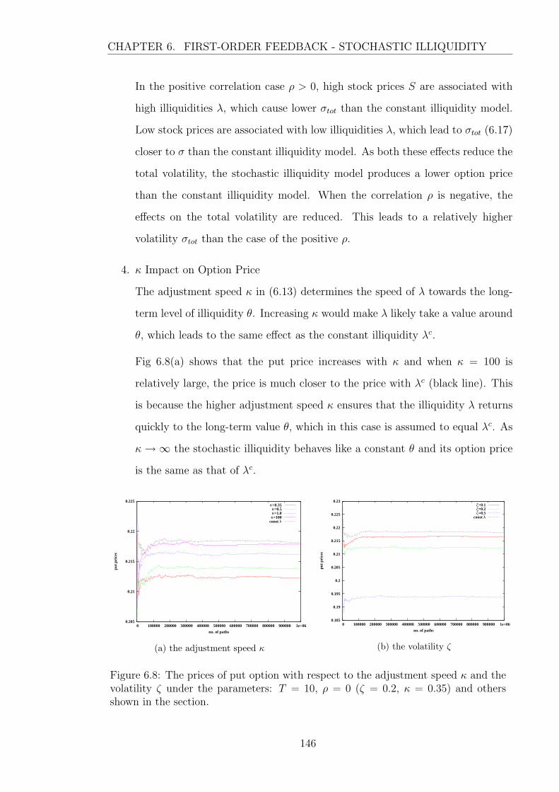
CHAPTER 6. FIRST-ORDER FEEDBACK - STOCHASTIC ILLIQUIDITY
In the positive correlation case ρ > 0, high stock prices S are associated with
high illiquidities λ, which cause lower σtot than the constant illiquidity model.
Low stock prices are associated with low illiquidities λ, which lead to σtot (6.17)
closer to σ than the constant illiquidity model. As both these effects reduce the
total volatility, the stochastic illiquidity model produces a lower option price
than the constant illiquidity model. When the correlation ρ is negative, the
effects on the total volatility are reduced. This leads to a relatively higher
volatility σtot than the case of the positive ρ.
4. κ Impact on Option Price
The adjustment speed κ in (6.13) determines the speed of λ towards the long-
term level of illiquidity θ. Increasing κ would make λ likely take a value around
θ, which leads to the same effect as the constant illiquidity λc.
Fig 6.8(a) shows that the put price increases with κ and when κ = 100 is
relatively large, the price is much closer to the price with λc (black line). This
is because the higher adjustment speed κ ensures that the illiquidity λ returns
quickly to the long-term value θ, which in this case is assumed to equal λc. As
κ→∞ the stochastic illiquidity behaves like a constant θ and its option price
is the same as that of λc.
0.205
0.21
0.215
0.22
0.225
0 100000 200000 300000 400000 500000 600000 700000 800000 900000 1e+06
put
pric
es
no. of paths
κ=0.35κ=0.5κ=1.0κ=100
const λ
(a) the adjustment speed κ
0.185
0.19
0.195
0.2
0.205
0.21
0.215
0.22
0.225
0.23
0 100000 200000 300000 400000 500000 600000 700000 800000 900000 1e+06
put
pric
es
no. of paths
ζ=0.1ζ=0.2ζ=0.5
const λ
(b) the volatility ζ
Figure 6.8: The prices of put option with respect to the adjustment speed κ and thevolatility ζ under the parameters: T = 10, ρ = 0 (ζ = 0.2, κ = 0.35) and othersshown in the section.
146

CHAPTER 6. FIRST-ORDER FEEDBACK - STOCHASTIC ILLIQUIDITY
5. ζ Impact on Option Price
The volatility of the illiquidity ζ refers to the deviation of random variables λ
from the long-term value θ. Then, compared with κ, ζ has the opposite effect
on pricing option, i.e. the price is clearly decreasing as ζ increases. As shown in
Fig 6.8(b), for ζ = 0.1, 0.2 and 0.5, the highest put price is given by the lowest
volatility ζ = 0.1, moreover the constant illiquidity λc yields the highest price
than others ζ. In fact, the constant illiquidity case can be obtained by setting
ζ = 0 assuming θ = λ0, because Eq (6.14) employed to simulate the illiquidity
process reduces to:
λj(ti+1) = λj(ti) = λ0 ,
for i = 0, · · · , N −1, which is equal to the value of λc in the constant illiquidity
model.
From the above we can see that all of the parameters can cause a difference in
option prices between the stochastic illiquidity model and the constant illiquidity
model, especially the maturity T which mainly determines if the prices given by the
stochastic illiquidity model are higher than those from the constant case. However
the stochastic illiquidity parameters, such as κ and ζ, just have a relatively modest
effect on the option pricing as the differences are somewhat small. Moreover, we also
find that the constant illiquidity is a specific case of the stochastic illiquidity process
when we choose larger κ, lower ζ or more negative correlation ρ.
6.2.3 Illiquidity θ impact on pricing option
As we mentioned before, in order to make the stochastic illiquidity model and the
constant illiquidity model comparable, we assume the long term illiquidity θ and the
initial value λ0 have the same value as the constant illiquidity λc and, i.e. λc = θ = λ0.
With respect to the impact of the stochastic illiquidity on the option prices, we focus
on the price’s sensitivity to the value of θ. Because only the European put option
interests us, no caps are applied to the model here. As the maturity T is an important
factor in affecting the differences in put prices between both models, we also test the
147

CHAPTER 6. FIRST-ORDER FEEDBACK - STOCHASTIC ILLIQUIDITY
option price behaviour with respect to varying maturities in Fig 6.9, which are the
close-to-expiry option with T = 0.1, the short-term option with T = 1 and the long-
term option with T = 10. The other parameters chosen for the examples in the
section are similar to those used in the previous sections, as follows: S1 = K = 0,
r = 0.04, σ = 0.2, ρ = 0, κ = 0.35, ζ = 0.2, N = 2000 and M = 106.
0
0.05
0.1
0.15
0.2
0.25
1 2 3 4 5 6 7 8 9 10
put
pric
e
θ (λc)
T=10T=1.0T=0.1
-0.015
-0.01
-0.005
0
0.005
0.01
0.015
0.02
1 2 3 4 5 6 7 8 9 10
Pst
och-
Pco
nst
θ (λc)
T=0.1T=1.0T=10
Figure 6.9: Pricing a European put option depends on long-term illiquidity θ (or λc)with different maturity T = 0.1, 1.0 and 10 in the left panel. The correspondingdifferences in the put prices between two models are given in the right panel, whichis calculated by the formula Pstoch − Pconst. The thicker line indicates the stochasticilliquidity model and the thinner line for the constant illiquidity model. θ is taken as0.1, 0.2, 0.3, · · · , 9.9, 1.0
We notice in the right panel of Fig 6.9 that the option prices estimated by both
models with a fixed maturity T are slightly different and the largest difference is less
than 0.02, which shows that the stochastic illiquidity does not significantly influence
the option value. For either option with short-term maturities or larger values of θ,
there is no difference between the two option prices, which indicates that both models
have the same price impact in such situations. From the left panel of Fig 6.9, for each
T there is an approximately skewed bell-shaped curve of option prices with respect
to θ (or λc for the constant illiquidity model), which is increasing in θ before the peak
price is reached at some θ∗ and afterwards the option price is generally decreasing in
θ as the variance of the underlying is relatively small. The right panel also indicates
that there are more significant differences when θ takes a value around θ∗. The value
of θ∗ is clearly relative to the maturity T and following the result in Section 5.2.3, θ∗
148
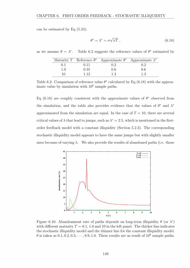
CHAPTER 6. FIRST-ORDER FEEDBACK - STOCHASTIC ILLIQUIDITY
can be estimated by Eq (5.24):
θ∗ = λ∗ = σ√πT , (6.18)
as we assume θ = λc. Table 6.2 suggests the reference values of θ∗ estimated by
Maturity T Reference θ∗ Approximate θ∗ Approximate λ∗
0.1 0.11 0.2 0.21.0 0.35 0.6 0.610 1.12 1.3 1.3
Table 6.2: Comparison of reference value θ∗ calculated by Eq (6.18) with the approx-imate value by simulation with 106 sample paths.
Eq (6.18) are roughly consistent with the approximate values of θ∗ observed from
the simulation, and the table also provides evidence that the values of θ∗ and λ∗
approximated from the simulation are equal. In the case of T = 10, there are several
critical values of λ that lead to jumps, such as λc = 2.5, which is mentioned in the first-
order feedback model with a constant illiquidity (Section 5.2.3). The corresponding
stochastic illiquidity model appears to have the same jumps but with slightly smaller
sizes because of varying λ. We also provide the results of abandoned paths (i.e. those
0
5
10
15
20
25
30
35
40
45
1 2 3 4 5 6 7 8 9 10
aban
donm
ent
rate
(%
)
θ (λc)
T=10T=1.0T=0.1
Figure 6.10: Abandonment rate of paths depends on long-term illiquidity θ (or λc)with different maturity T = 0.1, 1.0 and 10 in the left panel. The thicker line indicatesthe stochastic illiquidity model and the thinner line for the constant illiquidity model.θ is taken as 0.1, 0.2, 0.3, · · · , 9.9, 1.0. These results are as result of 106 sample paths.
149

CHAPTER 6. FIRST-ORDER FEEDBACK - STOCHASTIC ILLIQUIDITY
paths with negative prices) during the simulation in Fig 6.10. The abandonment rate
has a skewed bell-shaped curve excluding some kinks, which is similar to the option
price curve in the left panel of Fig 6.9. This is because a higher abandonment rate
implies a higher volatility of the underlying, which increases the option prices.
6.3 First-order feedback wrap-up
Chapters 5 and 6 have introduced and analyzed first-order feedback models with
constant and stochastic illiquidity parameter using a Monte Carlo simulation. To
implement the simulation, we require some additional restrictions on the simulation
process due to a problematic denominator of the volatility term in the feedback
models. The sensitivity of the option price to different parameters has been discussed
for each model and the comparison of option prices given by the both models are
presented as well. We also investigate put-call parity in these first-order feedback
models and provide an approach to decrease the error from put-call parity occurring
in the model simulation. The problem is mainly caused by mispricing call options,
hence we suggest to calculate the call option price using the corresponding put option
price.
Following the analysis of the first-order feedback models, in the next chapter we
will present a detailed analysis of the full feedback models in a simulation study.
150

Chapter 7
Full Feedback Model with
Constant Illiquidity
In this chapter we move to study an even more challenging model: a full feedback
model which is used to describe the situation in which traders realize that the market
is not perfectly liquid and perform the hedge according to a modified asset model.
The full feedback SDE has been derived by
dS = rSdt+σS
1− λSVSS
dWS , (7.1)
where the term VSS is derived by the modified SDE itself rather than by the Black-
Scholes formula, which leads to more difficulties in the implementation than the case
of the first-order feedback models discussed in the previous chapters; the illiquidity
coefficient λ is initially assumed to be constant. Following the analysis in Glover
(2008), the related non-linear PDE to the full feedback problem is
∂V
∂t+
1
2
σ2S2
(1− λSVSS)2
∂2V
∂S2+ rS
∂V
∂S− rV = 0 . (7.2)
Here, we will illustrate how to use the Monte Carlo method to simulate the path
following the stochastic process (7.1).
151
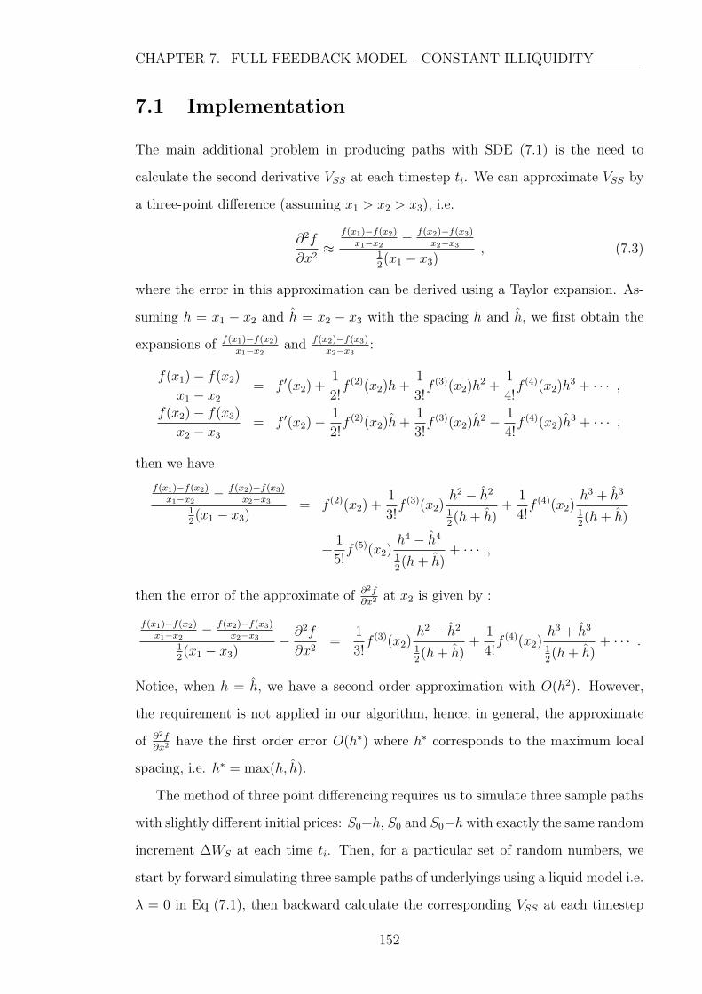
CHAPTER 7. FULL FEEDBACK MODEL - CONSTANT ILLIQUIDITY
7.1 Implementation
The main additional problem in producing paths with SDE (7.1) is the need to
calculate the second derivative VSS at each timestep ti. We can approximate VSS by
a three-point difference (assuming x1 > x2 > x3), i.e.
∂2f
∂x2≈
f(x1)−f(x2)x1−x2
− f(x2)−f(x3)x2−x3
12(x1 − x3)
, (7.3)
where the error in this approximation can be derived using a Taylor expansion. As-
suming h = x1 − x2 and h = x2 − x3 with the spacing h and h, we first obtain the
expansions of f(x1)−f(x2)x1−x2
and f(x2)−f(x3)x2−x3
:
f(x1)− f(x2)
x1 − x2
= f ′(x2) +1
2!f (2)(x2)h+
1
3!f (3)(x2)h
2 +1
4!f (4)(x2)h
3 + · · · ,f(x2)− f(x3)
x2 − x3
= f ′(x2)− 1
2!f (2)(x2)h+
1
3!f (3)(x2)h
2 − 1
4!f (4)(x2)h
3 + · · · ,
then we have
f(x1)−f(x2)x1−x2
− f(x2)−f(x3)x2−x3
12(x1 − x3)
= f (2)(x2) +1
3!f (3)(x2)
h2 − h2
12(h+ h)
+1
4!f (4)(x2)
h3 + h3
12(h+ h)
+1
5!f (5)(x2)
h4 − h4
12(h+ h)
+ · · · ,
then the error of the approximate of ∂2f∂x2 at x2 is given by :
f(x1)−f(x2)x1−x2
− f(x2)−f(x3)x2−x3
12(x1 − x3)
− ∂2f
∂x2=
1
3!f (3)(x2)
h2 − h2
12(h+ h)
+1
4!f (4)(x2)
h3 + h3
12(h+ h)
+ · · · .
Notice, when h = h, we have a second order approximation with O(h2). However,
the requirement is not applied in our algorithm, hence, in general, the approximate
of ∂2f∂x2 have the first order error O(h∗) where h∗ corresponds to the maximum local
spacing, i.e. h∗ = max(h, h).
The method of three point differencing requires us to simulate three sample paths
with slightly different initial prices: S0+h, S0 and S0−h with exactly the same random
increment ∆WS at each time ti. Then, for a particular set of random numbers, we
start by forward simulating three sample paths of underlyings using a liquid model i.e.
λ = 0 in Eq (7.1), then backward calculate the corresponding VSS at each timestep
152

CHAPTER 7. FULL FEEDBACK MODEL - CONSTANT ILLIQUIDITY
ti. Making use of the results of VSS, we reproduce the three sample paths under the
illiquid model of Eq (7.1), we then calculate VSS from these three paths at each time
point ti and the option value V (0) at initial time. The process is iterated using these
renewal values of VSS for each time to obtain a convergent value of V (0). Then the
final set of VSS is accepted by the particular set of random numbers. We then take
the average of a (large) number of estimators of V (0) from different sets of random
numbers. The general algorithm for a European call option is presented as follows:
1. Set up a discrete time framework by dividing the option’s life T into N time
steps, i.e. ti for i = 0, 1, · · · , N with t0 = 0, tN = T and equal increments
ti = ti−1 + ∆t. Suppose there are M sample paths in total, let j be the j-th
time of the simulation with j = 1, 2, ·,M . There would be some abandoned
paths during the simulation for three reasons: the underlying price is negative;
the prices of the three sample paths cross at some time; and the convergent
value V (0) cannot be achieved for some set of random numbers. Therefore, a
counter m, with m = 0 at the beginning of the simulation is used to check the
number of abandoned paths during the whole simulation.
2. Initialize VSS using Eq (7.1) when λ = 0
• choose one set of standard normal random variables for the j-th run of the
simulation (j ≤M): Zj(ti) for i = 0, 1, · · · , N − 1.
• to calculate VSS(ti) by the finite-difference method, we have to concur-
rently produce three sample paths S+j (ti), Sj(ti) and S−j (ti) rather than
one path in the first-order feedback case (and standard Monte Carlo com-
putation). Those paths can be simulated by a simple Euler discretization
as follows:
S+j (ti+1) = S+
j (ti) + rS+j (ti)∆t+ σS+
j (ti)Zj(ti)√
∆t ,
Sj(ti+1) = Sj(ti) + rSj(ti)∆t+ σSj(ti)Zj(ti)√
∆t ,
S−j (ti+1) = S−j (ti) + rS−j (ti)∆t+ σS−j (ti)Zj(ti)√
∆t ,
153

CHAPTER 7. FULL FEEDBACK MODEL - CONSTANT ILLIQUIDITY
where i = 0, 1, · · · , N − 1 and
S+j (t0) = S0 + h , Sj(t0) = S0 and S−j (t0) = S0 − h
for some small increment h serves as a price space for the underlying.
Notice that each path uses the same random variable Zj(ti) at time point
ti. Then the prices of a call option at time ti can be directly evaluated for
each path, which are:
V +j (ti) = e−r(T−ti) max
(S+
j (tN)−K, 0), (7.4)
Vj(ti) = e−r(T−ti) max(Sj(tN)−K, 0
), (7.5)
V −j (ti) = e−r(T−ti) max
(S−j (tN)−K, 0
), (7.6)
with the strike price K and exponential discount factor e−r(T−ti).
• approximate the corresponding VSSj(ti) at time ti by the three point dif-
ference method, which is given by
VSSj(ti) =
V +j (ti)−Vj(ti)
S+j (ti)−Sj(ti)
− Vj(ti)−V −j (ti)
Sj(ti)−S−j (ti)
12
(S+
j (ti)− S−j (ti)) , (7.7)
for i = 0, 1, · · · , N−1. The error in this approximation is O(h2) as h→ 0.
Then we set these values of VSSj(tj) as initial values used to simulate
SDE (7.1) with λ > 0.
3. Back to Eq (7.1) with a non-zero λ
• substitute the initial VSSj(ti) into Eq (7.1) and reproduce the three asset
paths as follows:
S+j (ti+1) = S+
j (ti) + rS+j (ti)∆t+
σS+j (ti)Zj(ti)
√∆t
1− λS+j (ti)VSSj
(ti), (7.8)
Sj(ti+1) = Sj(ti) + rSj(ti)∆t+σSj(ti)Zj(ti)
√∆t
1− λSj(ti)VSSj(ti)
, (7.9)
S−j (ti+1) = S−j (ti) + rS−j (ti)∆t+σS−j (ti)Zj(ti)
√∆t
1− λS−j (ti)VSSj(ti)
, (7.10)
where i = 0, 1, · · · , N − 1 and the same set of random variable Zj(ti) used
in Step 2. Similar to the first-order feedback model, the underlying prices
154

CHAPTER 7. FULL FEEDBACK MODEL - CONSTANT ILLIQUIDITY
from (7.8-7.10) could be negative when the term 1 − λSVSS in Eq (7.1)
is estimated to be nearly zero1. Therefore we discard the path by adding
the counter m to m+ 1 once its price becomes negative and set the value
of the option Vj(t0) = 0 for this run, then restart with the next run j + 1
from Step 2. Otherwise, we can directly obtain the prices of the call option:
V +j (ti), Vj(ti) and V −
j (ti) for each path at time ti from Eq (7.4) to Eq (7.6).
• calculate the new VSSj(ti) at each timestep by Eq (7.7) and record the
call price Vj(t0) at time zero. Notice that to avoid vanishing denominators
in Eq (7.7), any two values of the underlying prices: S+j (ti), Sj(ti) and
S−j (ti) cannot be the same. This was not a problem when λ = 0 in Step 2,
however for a non-zero λ, the underlying prices estimated by Eq (7.8-7.10)
could be nearly equal at some time ti. We discard the crossed path once
those values are equal and set m = m + 1 and Vj(t0) = 0, then restart
the next run from Step 2. When the prices of the underlying are nearly
equal, we would obtain a large value of VSSj(ti) (namely extreme values
of the Gamma), which could occur at any time ti rather than t → T in
the Black-Scholes formula. The extreme values of Gamma could cause a
sudden and considerable reduction in the total volatility of the underlying.
• repeat the above two steps to gain a new option price Vj(t0) until the
price Vj(t0) converges, i.e. the error between the current price and the
price received from last iteration is less than a prescribed tolerance ε =
10−5. In the algorithm we also set the maximum number of iterations as
Imax = 1000 to save computational costs and detect non-convergent paths.
If the current price Vj(t0) is convergent before the limit Imax is arrived, the
current price Vj(t0) is treated as the final price in the j-th run given by
the set of random variables Zj(ti); otherwise, we discard the nonconvergent
path and set the counter m = m+1 and Vj(t0) = 0, then move to the next
run j + 1 which starts from Step 2 with a new set of random variables.
1The term cannot be zero in a discrete time framework as mentioned in Chapter 5
155
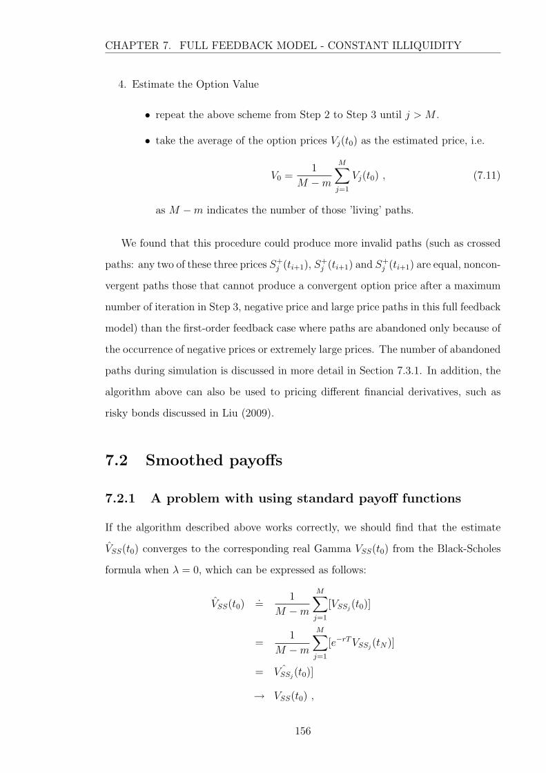
CHAPTER 7. FULL FEEDBACK MODEL - CONSTANT ILLIQUIDITY
4. Estimate the Option Value
• repeat the above scheme from Step 2 to Step 3 until j > M .
• take the average of the option prices Vj(t0) as the estimated price, i.e.
V0 =1
M −m
M∑j=1
Vj(t0) , (7.11)
as M −m indicates the number of those ’living’ paths.
We found that this procedure could produce more invalid paths (such as crossed
paths: any two of these three prices S+j (ti+1), S
+j (ti+1) and S+
j (ti+1) are equal, noncon-
vergent paths those that cannot produce a convergent option price after a maximum
number of iteration in Step 3, negative price and large price paths in this full feedback
model) than the first-order feedback case where paths are abandoned only because of
the occurrence of negative prices or extremely large prices. The number of abandoned
paths during simulation is discussed in more detail in Section 7.3.1. In addition, the
algorithm above can also be used to pricing different financial derivatives, such as
risky bonds discussed in Liu (2009).
7.2 Smoothed payoffs
7.2.1 A problem with using standard payoff functions
If the algorithm described above works correctly, we should find that the estimate
VSS(t0) converges to the corresponding real Gamma VSS(t0) from the Black-Scholes
formula when λ = 0, which can be expressed as follows:
VSS(t0).=
1
M −m
M∑j=1
[VSSj(t0)]
=1
M −m
M∑j=1
[e−rTVSSj(tN)]
= ˆVSSj(t0)]
→ VSS(t0) ,
156

CHAPTER 7. FULL FEEDBACK MODEL - CONSTANT ILLIQUIDITY
for M → ∞. However, due to the random occurrence of large values of VSS(t0), a
large number of sample paths are required to achieve the limit of VSS(t0) following
the algorithm with a standard payoff function. This can be shown in the left panel of
Fig 7.1(a) where a numerical example is used to illustrate how the estimate VSS(t0)
changes as M increases. In Fig 7.1(a), the estimate of VSS(t0) is nearly zero (around
-0.2
0
0.2
0.4
0.6
0.8
1
1.2
1.4
0 1e+06 2e+06 3e+06 4e+06 5e+06 6e+06 7e+06 8e+06 9e+06 1e+07 0
10000
20000
30000
40000
50000
60000
Est
imat
e of
VSS
(t0)
Indi
vidu
al V
SSj(t
0)
no. of paths
black-scholes formulaEstimate of VSS(t0)Individual VSSj
(t0)
(a) a standard payoff function f0(S, T )
0.25
0.3
0.35
0.4
0.45
0 100000 200000 300000 400000 500000 600000 700000 800000 900000 1e+06
VSS
(t0)
no. of paths
black-scholes formulaω=0.1ω=0.5ω=1.0
(b) a smoothing payoff function f1(S, T )
Figure 7.1: Estimate of VSS(t0) for a European call option in a perfect liquid market,i.e. λ = 0 with a standard payoff function f0(S, T ) = max(S(T ) −K, 0) in the left
panel and with a smoothing payoff function f1(S, T ) =K(S(T )−K+
√(S(T )−K)2+ω2)
K+√
K2+ω2 in
the right panel under the same parameter setting: S(t0) = K = 1, r = 0.04, σ = 0.2,T = 10, N = 2000.
10−5) at the beginning of the simulation and it abruptly jumps to a high level of
VSS(t0), followed by a general fall before the next jump occurs. This is because, for
each path j, the individual value of VSSj(ti) estimated by Eq (7.7) is always zero for
i = 0, 1, · · · , N − 1, except that those paths hit the strike price, K, i.e. satisfying the
condition S+j (tN) > K and S−j (tN) < K. These exceptions do not happen frequently,
as seen in the figure, but still result in a significant increase in the value of VSS(t0),
when there is a limit on the number of sample paths. Such jumps affect the speed
of the convergence of the estimated prices. Thus, from Fig 7.1(a), we see that 106
sample paths still cannot resolve the estimate of VSS(t0), compared to the benchmark
value given by the Black-Scholes formula. After 107 sample paths, the estimate of
VSS(t0) does indeed converge to the Black-Scholes price, because these jumps have
less impact on the estimate VSS(t0) over a significantly large number of sample paths.
157

CHAPTER 7. FULL FEEDBACK MODEL - CONSTANT ILLIQUIDITY
Therefore, we seek for a way of improving of the speed the convergence of the estimate
VSS(ti) for each time point, ti.
7.2.2 Resolution
The problem described above arises because the standard payoff function of a Eu-
ropean call option comprises two straight lines which intersect each other when
Sj(tN) = K. If these three paths S+j (ti), Sj(ti) and S−j (ti) expire either in the money
or out the money concurrently, then VSSj(t0) is equal to zero2. The only possibility
to gain a non-zero estimate of VSSj(t0) occurs when S+
j (tN), Sj(tN) and S−j (tN) do
not lie in the same line, i.e. the underlying price hits close to the strike price. In such
a situation, the non-zero Gamma is relatively large so that there are sharp jumps on
the average cumulative estimate VSS(t0) in the figure.
To overcome this limitation of the convergence, we use a sufficiently smooth payoff
function, which has a finite second derivative everywhere. We achieve this using a
smoothing function, that ensures we obtain non-zero VSS, which helps to enhance
the illiquidity effect on the stochastic process. Following Glover (2008), we assume
similar smoothing payoff functions with a parameter ω in Table 7.1. Compared with
Model f0(S, T ) f1(S, T ) f2(S, T )
European Call max(S −K, 0)K(S−K+
√(S−K)2+ω2)
K+√
K2+ω2
S−K+√
(S−K)2+ω2
2
European Put max(K − S, 0)K(K−S+
√(S−K)2+ω2)
K+√
K2+ω2
K−S+√
(S−K)2+ω2
2
Table 7.1: Smoothing payoff function for different derivatives used in Glover (2008)f2(S, T ) and our model f1(S, T ). The standard payoff function is defined as f0(S, T ).
the Glover’s payoff functions f2(S, T ) which is also used in Frey (1996), our payoff
f1(S, T ) is much closer to the value given by the standard payoff function, in particular
for the case of put options when the underlying price S = 0, where f1(S, T ) gives the
same value K as the standard payoff function whilst f2(S, T ) cannot (see Fig 7.2(b)).
Fig 7.2 provides the different payoffs’ change depends on the smoothing parameter
ω, where ω = 0.0, 0.4, 0.8 and 1.0. For European put options, both smoothed payoffs
2However, computer round-off error occurs in the calculation of VSSj (t0) for those paths withS−j (tN ) > K, which leads to a nearly zero estimate (around 10−5) rather than zero.
158

CHAPTER 7. FULL FEEDBACK MODEL - CONSTANT ILLIQUIDITY
0
0.5
1
1.5
2
2.5
0 0.5 1 1.5 2 2.5 3
Pay
off
of C
all
S
ω ↓ 0
f0(S,T)f1(S,T)f2(S,T)
(a) Call Option
0
0.2
0.4
0.6
0.8
1
1.2
1.4
0 0.5 1 1.5 2 2.5 3
Pay
off
of p
ut
S
ω ↓ 0
f0(S,T)f1(S,T)f2(S,T)
(b) Put Option
Figure 7.2: Different smoothing payoff functions depend on the illiquidity ω, whichare the standard payoff function f0(S, T ), Glover’s smoothed payoff f2(S, T ) and themodified smoothed payoff f1(S, T ).
are higher than the standard payoff value and strictly decreasing with decreases in
ω; for European call options, the payoff value f1(S, T ) shows different behaviours
with respect to ω in two region of S: for S < 2K, all values of f1(S, T ) lie above
the standard payoff f0(S, T ) and decreasing as ω reduces, whilst for S > 2K the
smoothed function f1(S, T ) lies below f0(S, T ) and increasing as ω reduces. We note
that the largest difference between the smoothing payoffs and the standard payoff
occurs at the singular point S = K. This indicates that the smoothing parameter ω
has significantly more impact on the pricing ATM options than DOTM and DITM
options. To apply the smoothed payoff f1(S, T ), we replace Eq (7.4)-(7.6) in Step 2
of Implementation (Section 7.1) with
V +j (ti) = e−r(T−ti)
K(S+
j (tN)−K +√
(S+j (tN)−K)2 + ω2
)
K +√K2 + ω2
,
Vj(ti) = e−r(T−ti)K
(Sj(tN)−K +
√(Sj(tN)−K)2 + ω2
)
K +√K2 + ω2
,
V −j (ti) = e−r(T−ti)
K(S−j (tN)−K +
√(S−j (tN)−K)2 + ω2
)
K +√K2 + ω2
.
Fig 7.1(b) shows the estimated values of Gamma VSS(t0) using the smoothed payoff
f1(S, T ). The convergence of the estimated VSS(t0), which used to be problematic in
the algorithm with the standard payoff f0(S, T ), has been greatly justified. As the
159
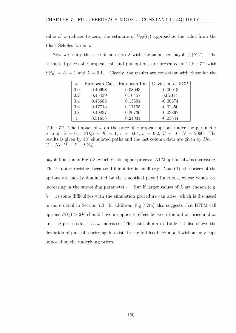
CHAPTER 7. FULL FEEDBACK MODEL - CONSTANT ILLIQUIDITY
value of ω reduces to zero, the estimate of VSS(t0) approaches the value from the
Black-Scholes formula.
Now we study the case of non-zero λ with the smoothed payoff f1(S, T ). The
estimated prices of European call and put options are presented in Table 7.2 with
S(t0) = K = 1 and λ = 0.1. Clearly, the results are consistent with those for the
ω European Call European Put Deviation of PCP0.0 0.40998 0.08043 -0.000130.2 0.45439 0.10457 0.020140.4 0.45688 0.13594 -0.008740.6 0.47713 0.17195 -0.024500.8 0.49837 0.20736 -0.038671 0.51658 0.24034 -0.05344
Table 7.2: The impact of ω on the price of European options under the parametersetting: λ = 0.1, S(t0) = K = 1, r = 0.04, σ = 0.2, T = 10, N = 2000. Theresults is given by 106 simulated paths and the last column data are given by Dev =C +Ke−rT − P − S(t0).
payoff function in Fig 7.2, which yields higher prices of ATM options if ω is increasing.
This is not surprising, because if illiquidity is small (e.g. λ = 0.1), the prices of the
options are mostly dominated by the smoothed payoff functions, whose values are
increasing in the smoothing parameter ω. But if larger values of λ are chosen (e.g.
λ = 1) some difficulties with the simulation procedure can arise, which is discussed
in more detail in Section 7.3. In addition, Fig 7.2(a) also suggests that DITM call
options S(t0) > 2K should have an opposite effect between the option price and ω,
i.e. the price reduces as ω increases. The last column in Table 7.2 also shows the
deviation of put-call parity again exists in the full feedback model without any caps
imposed on the underlying prices.
160

CHAPTER 7. FULL FEEDBACK MODEL - CONSTANT ILLIQUIDITY
7.3 Problems arising from smoothed function - fail-
ure paths
In this section, with respect to the deviation of put-call parity, we will concentrate
on European put options and focus on deeper analysis of failure paths when us-
ing smoothed payoff functions, computing with the dynamic of the underlying asset
S(t) in Eq (7.1) and the terminal condition f1(S, T ) of the European put V (S, t) in
Table 7.1.
The algorithm utilising a smoothed payoff function for the full feedback case was
found to lead to two phenomena: many more abandoned paths than the first-order
feedback model using the standard payoff function f(S, T ) in Table 7.1, and extremely
large values of the Gamma; the two phenomena are not unconnected. Because Monte
Carlo simulation is based on the law of large numbers, a high number of abandoned
paths does increase the cost of computation and can even contaminate the simulation,
with too many paths being unusable. Our studies show there exists a relation between
a smoothing parameter ω and the illiquidity parameter λ chosen to reduce the path
abandonment rate for the simulation.
7.3.1 Abandoned paths
We study the number of abandoned paths which lead to the difficulties in pricing
options. There are three standard rules to judge which paths should be discarded, as
explained in Section 7.1. One of these is the paths with negative or large prices due
to nearly vanishing denominators of the volatility term in (7.1), which are also found
in the first-order feedback model. Another is crossed paths, i.e. any two of the three
prices S+(tj), S(tj) and S−(tj) are nearly equal, which invalidates the calculation of
the Gamma. Another is the paths which cannot provide a convergent price for the
option (for example, the convergence could not be less than 10−6 after 1000 itera-
tions). To alleviate these failures of the algorithm, it is the best to abandon the paths
once they cross, go negative, are extremely large or lead to nonconvergent. At the
161

CHAPTER 7. FULL FEEDBACK MODEL - CONSTANT ILLIQUIDITY
same time, we count the number of abandoned paths out of all the simulated paths.
Fig 7.3 shows that the abandonment rate approaches some level as the number of
48.2
48.4
48.6
48.8
49
49.2
49.4
49.6
49.8
50
0 100000 200000 300000 400000 500000 600000 700000 800000 900000 1e+06
aban
donm
ent
rate
(%
)
no. of paths
Sample 1Sample 2Sample 3Sample 4Sample 5
Figure 7.3: Abandonment rate of paths in pricing a European put with S(t0) = K =1, r = 0.04, σ = 0.2, T = 10, λ = ω = 1 and N = 2000
paths increases, which the abandoned paths take up nearly 49% of all the paths in
the case λ = ω = 1. With the benefit of saving processing time, we can estimate
the abandonment rate after 105 paths run. Table 7.3 gives a detailed breakdown
of the abandonment rate when pricing a European put option. It is divided into
dt Abandonment Crossed Unconvergent Negative Over-Cap 101/200 49.19 27.00 0.06 74.24 n/a1/500 49.06 41.23 0.05 61.80 n/a1/1000 48.95 50.34 0.05 54.38 n/a
1/200 49.28 23.17 0.03 65.66 23.561/500 49.15 37.25 0.04 56.88 21.061/1000 49.03 46.68 0.03 51.13 19.37
Table 7.3: Three Causes & Four Causes Contribution to Abandonment Paths (%)for pricing a European put with S(t0) = K = 1, r = 0.04, σ = 0.2, T = 10, λ = ω = 1and N = 2000, 5000, 10000. The results are given by 106 simulations based on 64-bitmachines
two parts, which depend upon whether the over-capped price is considered or not.
We notice that the total number of abandoned paths does not change significantly if
sample paths with over-capped prices are discarded during the simulation. Without
162

CHAPTER 7. FULL FEEDBACK MODEL - CONSTANT ILLIQUIDITY
discarding the over-capped prices, the data shows an increase in the number of aban-
doned paths due to the other three reasons. This implies that the abandoned paths
with large prices are strictly related to the paths with negative prices, unconvergent
prices and nonconvergent prices. Thus, some of the results in the following tests are
obtained without discarding the paths with large prices.
Our experiment also confirms that abandoned paths are usually associated with
changes of the sign of the denominator, i.e. 1 − λSVSS in SDE (7.1), which is con-
sidered as an indicator. Fig 7.4 provides 16 independent samples with 106 paths
374000
375000
376000
377000
378000
379000
380000
1 2 3 4 5 6 7 8 9 10 11 12 13 14 15 16
no. o
f ab
ando
ned
path
s w
ith
sign
cha
nge
Sample
0
20
40
60
80
100
1 2 3 4 5 6 7 8 9 10 11 12 13 14 15 16
no. o
f liv
ing
path
s w
ith
sign
cha
nge
Sample
Figure 7.4: The number of abandoned (living) paths with the changes of the sign ofthe denominator pricing a European put with S(t0) = K = 1, r = 0.04, σ = 0.2,T = 10, λ = ω = 1 and N = 2000. Each sample is given by 106 paths.
each. The number of the living paths that experience sign change in the denominator
is normally less than 60 out of 106 sample paths, while those abandoned paths with
a sign change total more than 376000, which is a high percentage (around 80%) of
the total number of the abandoned paths. The results in Fig 7.4 show that the non-
abandoned paths rarely change their denominators’ signs, so it is intuitive to put some
constraint on the denominator to avoid abandoned paths, such as 1 − λSVSS > 0,
which is mentioned by Glover (2008) with the smoothing payoff function f2(S, T ) in
Table 7.1. We rewrite his model as:
dS = rSdt+σS
1− λVSS
dWS ,
V (S, T ) =1
2(K − S +
√(K − S)2 + ω2) ,
where the denominator of his SDE is 1 − λVSS, assuming the illiquidity function as
163

CHAPTER 7. FULL FEEDBACK MODEL - CONSTANT ILLIQUIDITY
the constant λ rather than λS in our model. By the maximum principle, Glover finds
a critical value of λ (i.e. λ = 2ω) and shows the condition:
λ < 2ω
can prevent the dominator of the volatility term from vanishing. Following similar
analysis, we derive the condition suitable for our case with the smoothing payoff
f1(S, T ), which is
λS < ω(1 +√
1 + (ω/K)2) .
Let the upper bound for underlying price S be S, then a relation between λ and ω is
given by
λ < ω(1 +√
1 + (ω/K)2)/S .
To demonstrate that this condition works well, Fig 7.5 illustrates abandonment rates
for pricing a put option for different values of λ and ω. Fig 7.5(b) is for Glover’s
0
2
4
6
8
10
0 2 4 6 8 10
λ
ω
10080604020αβ
(a) Our model
0
2
4
6
8
10
0 2 4 6 8 10
λ
ω
10080604020α
(b) Glover’s model
Figure 7.5: Contour figures of abandonment rate in the ω versus λ plane for pricinga European put with S = K = 1, r = 0.04, σ = 0.2, T = 10, N = 2000 and S = 10.The red dash lines α stand for the condition line α : λ = 2ω while the black curve βstands for the condition line β : λ = ω(1 +
√1 + (ω/K)2)/S. The data is given by
105 sample paths.
(2008) model and Fig 7.5(a) is ours. The contour lines with 100 correspond to 100%
abandonment rate and are located in the upper-left corners of both graphs, which
means the points (λ, ω) lying in this area would bear the highest risk of abandonment.
In the remainder of the domain, the abandonment rate is generally declining and the
164

CHAPTER 7. FULL FEEDBACK MODEL - CONSTANT ILLIQUIDITY
‘safest’ points appear in the lower-right corner where the abandonment rate is less
than 20%. In Fig 7.5, by comparison with the condition line α given by λ = 2ω and
the line β given by λ = ω(1+√
1 + (ω/K)2)/S, we can easily find that the condition
λ < 2ω excludes the contour lines with 100% rates as both of them are above the
condition line α. Moreover, we can apply the condition λ < ω(1 +√
1 + (ω/K)2)/S
in Fig 7.5(a), and this condition ensures the maximum abandonment rate is less than
60%. From the two contour graphs, we can generally say that Fig 7.5(a) has fewer
discarded paths because the blank area below the blue contour line with 20% is much
larger than that on the right. This means our model has an advantage of producing
valid paths over Glover’s model in the simulation study.
As for the discrete-time model we study here, the size of the time-step is also
a factor increasing the number of abandoned paths. One way to overcome this is
naturally to choose sufficiently small time-steps. For our full feedback model, Ta-
ble 7.3 shows that the percentage of the total of abandoned paths is reduced slightly
by reducing the time-steps ∆t, but its effect is not significant. According to the rea-
sons for abandoning paths, i.e. those that are crossed paths, nonconvergent paths,
negative paths or over-capped paths, we found that reducing time-steps ∆t would
lead to an obvious decline in the number of negative and overcap paths as we might
expect, but it would also increase the number of crossed paths. As a result, the total
abandonment rates remain at the same level. In addition, nonconvergent paths are
too infrequent to be considered here.
We also examine how the moneyness of options would change abandonment rates.
As shown in Fig 7.6, for the fixed strike price K = 1, the abandonment rate can be
shown as a convex-shape curve with respect to the spot price S, with the peak around
S = 0.7, which indicates that ITM options (even ATM options) are more likely to
produce the abandoned paths whilst DITM options are not. This is because for
DITM options, the smoothing payoff function is much closer to the standard payoff
function (see Fig 7.2(b)), then the value of VSS is too small to significantly reflect
the impact of the illiquidity on the underlying process. Besides the moneyness, we
consider two numerical parameters in the algorithm, the increment of spot prices h
165

CHAPTER 7. FULL FEEDBACK MODEL - CONSTANT ILLIQUIDITY
0
20
40
60
80
100
0 0.2 0.4 0.6 0.8 1 1.2 1.4 1.6 1.8 2ab
ando
ned
path
s (%
)
S
Figure 7.6: Abandonment rate of paths with different S when pricing a Europeanput with K = 1, r = 0.04, σ = 0.2, T = 10, N = 2000 and λ = ω = 1
and the tolerator ε for judging the convergence of the pricing. Table (7.4) indicates
h nearly has a little effect on the abandonment rate, whilst the rate increases slightly
by reducing ε.
Abandonment Increment h Abandonment Tolerator εRate 10−1 10−3 10−5 Rate 10−3 10−4 10−5 10−6
(%) 49.54 49.33 49.32 (%) 45.71 48.92 49.67 56.41
Table 7.4: Abandonment rate of paths with different h & ε when pricing a Europeanput with S = K = 1, r = 0.04, σ = 0.2, T = 10, N = 2000 and λ = ω = 1
7.3.2 Extreme values of Gamma
In this section, we describe more details on the interesting phenomenon of extreme
large values of Gamma. When calculating Gammas by Eq (7.7), as mentioned in
Section 7.1 we note that the denominator could be small enough to result in abnor-
mally large values of Gamma when the paths become close. Fig 7.7 illustrates how
this situation happens. In the left panel, we monitor a particular path with a large
Gamma appearing around t = 7. The corresponding difference: S+ − S, S − S− and
12(S+−S−) given in the right panel suggests the smallest absolute difference (around
2.5× 10⁻⁸) should occur around t = 7 (indicated by an arrow in the figure), which is
consistent with the time when extreme values of Gamma show up in the left panel.
Actually, the extreme values of Gamma are caused by the smallest multiplication
of these differences: |(S+ − S)(S+ − S−)(S − S−)|min, rather than the differences
166

CHAPTER 7. FULL FEEDBACK MODEL - CONSTANT ILLIQUIDITY
0
5
10
15
20
25
30
35
40
45
0 1 2 3 4 5 6 7 8 9 10
Gam
me
time t
0
1e-05
2e-05
3e-05
4e-05
5e-05
6e-05
7e-05
0 1 2 3 4 5 6 7 8 9 10
Diff
eren
ce o
f S
time t
|S-S-|0.5|S+-S-|
|S+-S|
0
2e-07
4e-07
6.8 7 7.2 7.4 7.6 7.8 8
Figure 7.7: A particular path with extreme values of Gamma in pricing a Europeanput with S = K = 1, r = 0.04, σ = 0.2, T = 10, λ = ρ = 1 and N = 2000
themselves: |(S+−S)|min, |(S+−S−)|min or |(S−S−)|min. Fig 7.8 gives an example
to illustrate this point. For a particular path with extreme values of Gamma, in the
left panel, we plot the values of Gamma against the individually differences: (S+−S),
(S − S−) and 12(S+ − S−). Most values of Gamma are significantly larger when the
S values are close, but in this region we still find there are relatively small values of
Gamma. Meanwhile, we can check the product of these differences for the same path
in the right panel of Fig 7.8. When the product of differences is close to zero, the
values of Gamma are certainly quite large. Hence, we can deduce that extreme values
of Gamma can only be produced by the smallest value of |(S+ − S)(S+ − S−)(S −S−)|min.
-20
0
20
40
60
80
100
120
140
160
180
200
-0.0004 -0.0003 -0.0002 -0.0001 0 0.0001 0.0002 0.0003
Gam
ma
Difference of S
(S+-S)0.5(S+-S-)
(S-S-)
-20
0
20
40
60
80
100
120
140
160
180
200
-6e-11 -5e-11 -4e-11 -3e-11 -2e-11 -1e-11 0 1e-11 2e-11 3e-11 4e-11
Gam
ma
Difference of S
(S+-S)(S+-S-)(S-S-)
Figure 7.8: A particular path with extreme values of Gamma in pricing a Europeanput with S = K = 1, r = 0.04, σ = 0.2, T = 10, λ = ρ = 1 and N = 2000
167

CHAPTER 7. FULL FEEDBACK MODEL - CONSTANT ILLIQUIDITY
The main effect of the extreme values of Gamma on the asset process is to elimi-
nate the volatility term of SDE (7.1) and change the risky asset to the riskless asset.
For instance, the underlying price shown in the left panel of Fig 7.9 moves like a
riskless asset before t = 5.5 and then follows a stochastic process. This strange move-
ment is explained by the right panel, which shows the existence of extreme values
of Gamma in the corresponding time horizon. The ‘Extra Values of Gamma Effect’
could be used to realize more specific financial circumstance in practise. Moreover,
0.4
0.6
0.8
1
1.2
1.4
1.6
0 1 2 3 4 5 6 7 8 9 10
Und
erly
ing
Pric
e
time t
S-
SS+
riskless asset
0
20000
40000
60000
80000
100000
120000
0 1 2 3 4 5 6 7 8 9 10
Gam
ma
time t
Figure 7.9: A particular path with extreme values of Gamma in pricing a Europeanput with S = K = 1, r = 0.04, σ = 0.2, T = 10, λ = ρ = 1 and N = 2000
Fig 7.10(a) describes a cumulative distribution of extreme values of Gamma on dif-
ferent time intervals using 105 sample paths. The histogram has a lower peak in the
middle, and higher values on the right side than the left side, which means it is more
likely that extreme values of Gamma occur when options are close to maturity. We
also investigate the maximum size of the Gammas along each path. The result pre-
sented in the Fig 7.10(b) shows the largest concentration of Gammas is in the range
[10 : 100], and the observation of extremely large values of Gamma (larger than 105)
is rare.
The extreme values of Gamma effect also contributes to the number of abandoned
paths in the algorithm. Once the value of Gamma was extremely large (for example
|VSS(ti)| > 100), the denominator always changed from positive to negative. As
mentioned earlier in Section 7.3.1, a change in sign of the denominator 1 − λSVSS
in the simulation would usually be found in abandoned paths rather than living
168

CHAPTER 7. FULL FEEDBACK MODEL - CONSTANT ILLIQUIDITY
0
5000
10000
15000
20000
0 1 2 3 4 5 6 7 8 9 10
quan
tity
in 1
0000
0 sa
mpl
es
time
(a) A cumulative distribution of the amountof extreme values of Gamma.
0
500
1000
1500
2000
2500
3000
3500
4000
4500
5000
10+2010201019101810171016101510141013101210111010109108107106105104103102101
quan
tity
Gamma size
(b) A cumulative distribution of Gammasizes.
Figure 7.10: A test by 105 sample paths with S = K = 1, r = 0.04, σ = 0.2, T =10, λ = ρ = 1 and N = 2000
paths. For large values of Gamma (says 10 ≤ VSS(ti) ≤ 100), if the sign does not
change, we can still suppose that these Gammas allow more chances for a nearly zero
denominator: 1 − λSVSS → 0, which could lead to a abandoned path. In such a
case, there would be a significant increase in the volatility term, which would make
the underlying price suddenly rise above a common price level or drop to a negative
price. When there is a drop in the underlying price, the order of S+ > S > S− would
be disrupted, as the highest price S+ reduces more sharply than the other two, so
these three paths would be more lively to cross each other (intersect) in the future
simulation. Consider both the range of the extreme values of Gamma. Intuitionally,
we may anticipate there exists a relationship between the extreme values of Gamma
and the number of abandoned paths. Fig 7.11 indicates the number of abandoned
paths and the number of living paths associated with extreme values of Gamma over
total 106 sample paths in multiple independent tests (17 times). Similar to the
results of the sign of the denominator shown in Fig 7.4, we find that in the 106
simulation paths for each test, there were few living paths with extreme values of
Gamma (less than 60) but a large number of the abandoned paths with extreme
values of Gamma, which is higher than 50% of the total number of the abandoned
paths. This strongly suggests that most paths where large values of Gamma occur
could always be abandoned.
169

CHAPTER 7. FULL FEEDBACK MODEL - CONSTANT ILLIQUIDITY
285000
286000
287000
288000
289000
290000
1 2 3 4 5 6 7 8 9 10 11 12 13 14 15 16
no. o
f ab
ando
ned
path
s w
ith
big
Gam
ma
Sample
0
20
40
60
80
100
1 2 3 4 5 6 7 8 9 10 11 12 13 14 15 16
no. o
f liv
ing
path
s w
ith
big
Gam
ma
Sample
Figure 7.11: The number of abandoned (living) paths with extreme values of Gammain pricing a European put with S(t0) = K = 1, r = 0.04, σ = 0.2, T = 10, λ = ω = 1and N = 2000. Each sample is given by 106 paths.
7.4 Illiquidity λ impact on pricing option
In this section, we investigate an impact of illiquidity on the option prices using a
standard payoff or a smoothed payoff. We also check if estimated prices of call and
put options satisfy put-call parity. As shown in Glover (2008), put-call parity should
still hold in the full feedback model. Following PDE (7.2), we find that the non-linear
PDE differs from the standard Black-Scholes PDE only as the volatility term, which
is a function of the stock price and the second derivatives for the option price, i.e.
σ = σ(t, S, VSS). Since the second derivative of the put and call options coincide, the
put-call parity should still hold in our full feedback model.
7.4.1 Option pricing with standard payoffs
We start with illiquidity λ effects on pricing European options with standard payoff
functions f0(S, T ) in Table 7.1. As mentioned in Section 7.2, the standard payoffs
can cause extremely small values of Gamma, which will eliminate illiquidity effects
on pricing options. Fig 7.12 shows how the option price changes with respect to
the different λ (0, 0.5, 1, 3 and 5) under the parameter setting: S = K = 1, r = 0.04,
σ = 0.2, T = 10, N = 2000 and h = ε = 10−5. Even without any caps on underlying
prices, both option prices converge to a particular value as the number of paths
M increases, which indicates our algorithm is reliable and valid. It also suggests
170
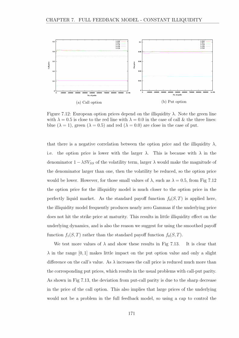
CHAPTER 7. FULL FEEDBACK MODEL - CONSTANT ILLIQUIDITY
0
0.1
0.2
0.3
0.4
0.5
0 100000 200000 300000 400000 500000 600000 700000 800000 900000 1e+06
Cal
l pri
ce
No. of paths
λ=0.0λ=0.5λ=1.0λ=3.0λ=5.0
(a) Call option
0
0.02
0.04
0.06
0.08
0.1
0 100000 200000 300000 400000 500000 600000 700000 800000 900000 1e+06
Put
pri
ce
No. of paths
λ=0.0λ=0.5λ=1.0λ=3.0λ=5.0
(b) Put option
Figure 7.12: European option prices depend on the illiquidity λ. Note the green linewith λ = 0.5 is close to the red line with λ = 0.0 in the case of call & the three lines:blue (λ = 1), green (λ = 0.5) and red (λ = 0.0) are close in the case of put.
that there is a negative correlation between the option price and the illiquidity λ,
i.e. the option price is lower with the larger λ. This is because with λ in the
denominator 1−λSVSS of the volatility term, larger λ would make the magnitude of
the denominator larger than one, then the volatility be reduced, so the option price
would be lower. However, for those small values of λ, such as λ = 0.5, from Fig 7.12
the option price for the illiquidity model is much closer to the option price in the
perfectly liquid market. As the standard payoff function f0(S, T ) is applied here,
the illiquidity model frequently produces nearly zero Gammas if the underlying price
does not hit the strike price at maturity. This results in little illiquidity effect on the
underlying dynamics, and is also the reason we suggest for using the smoothed payoff
function f1(S, T ) rather than the standard payoff function f0(S, T ).
We test more values of λ and show these results in Fig 7.13. It is clear that
λ in the range [0, 1] makes little impact on the put option value and only a slight
difference on the call’s value. As λ increases the call price is reduced much more than
the corresponding put prices, which results in the usual problems with call-put parity.
As shown in Fig 7.13, the deviation from put-call parity is due to the sharp decrease
in the price of the call option. This also implies that large prices of the underlying
would not be a problem in the full feedback model, so using a cap to control the
171
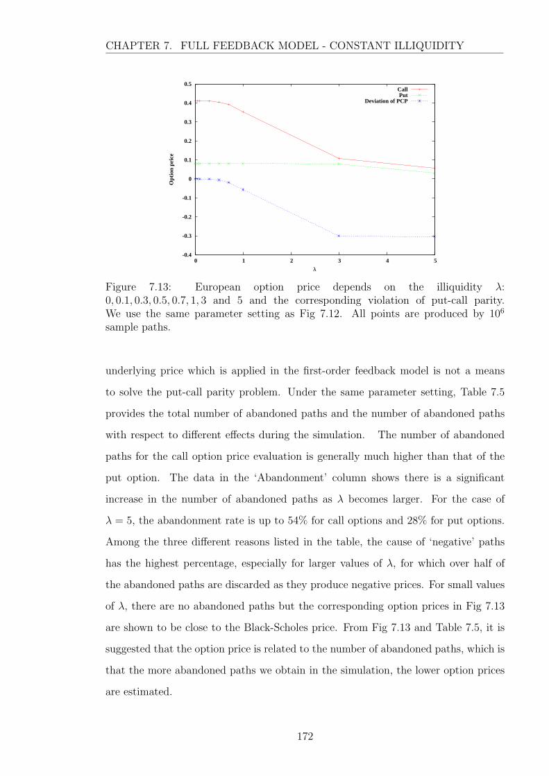
CHAPTER 7. FULL FEEDBACK MODEL - CONSTANT ILLIQUIDITY
-0.4
-0.3
-0.2
-0.1
0
0.1
0.2
0.3
0.4
0.5
0 1 2 3 4 5
Opt
ion
pric
e
λ
CallPut
Deviation of PCP
Figure 7.13: European option price depends on the illiquidity λ:0, 0.1, 0.3, 0.5, 0.7, 1, 3 and 5 and the corresponding violation of put-call parity.We use the same parameter setting as Fig 7.12. All points are produced by 106
sample paths.
underlying price which is applied in the first-order feedback model is not a means
to solve the put-call parity problem. Under the same parameter setting, Table 7.5
provides the total number of abandoned paths and the number of abandoned paths
with respect to different effects during the simulation. The number of abandoned
paths for the call option price evaluation is generally much higher than that of the
put option. The data in the ‘Abandonment’ column shows there is a significant
increase in the number of abandoned paths as λ becomes larger. For the case of
λ = 5, the abandonment rate is up to 54% for call options and 28% for put options.
Among the three different reasons listed in the table, the cause of ‘negative’ paths
has the highest percentage, especially for larger values of λ, for which over half of
the abandoned paths are discarded as they produce negative prices. For small values
of λ, there are no abandoned paths but the corresponding option prices in Fig 7.13
are shown to be close to the Black-Scholes price. From Fig 7.13 and Table 7.5, it is
suggested that the option price is related to the number of abandoned paths, which is
that the more abandoned paths we obtain in the simulation, the lower option prices
are estimated.
172
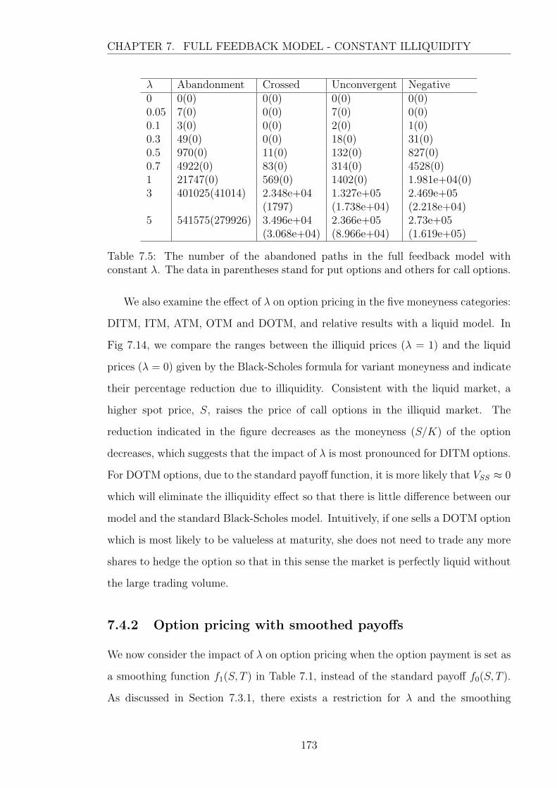
CHAPTER 7. FULL FEEDBACK MODEL - CONSTANT ILLIQUIDITY
λ Abandonment Crossed Unconvergent Negative0 0(0) 0(0) 0(0) 0(0)0.05 7(0) 0(0) 7(0) 0(0)0.1 3(0) 0(0) 2(0) 1(0)0.3 49(0) 0(0) 18(0) 31(0)0.5 970(0) 11(0) 132(0) 827(0)0.7 4922(0) 83(0) 314(0) 4528(0)1 21747(0) 569(0) 1402(0) 1.981e+04(0)3 401025(41014) 2.348e+04 1.327e+05 2.469e+05
(1797) (1.738e+04) (2.218e+04)5 541575(279926) 3.496e+04 2.366e+05 2.73e+05
(3.068e+04) (8.966e+04) (1.619e+05)
Table 7.5: The number of the abandoned paths in the full feedback model withconstant λ. The data in parentheses stand for put options and others for call options.
We also examine the effect of λ on option pricing in the five moneyness categories:
DITM, ITM, ATM, OTM and DOTM, and relative results with a liquid model. In
Fig 7.14, we compare the ranges between the illiquid prices (λ = 1) and the liquid
prices (λ = 0) given by the Black-Scholes formula for variant moneyness and indicate
their percentage reduction due to illiquidity. Consistent with the liquid market, a
higher spot price, S, raises the price of call options in the illiquid market. The
reduction indicated in the figure decreases as the moneyness (S/K) of the option
decreases, which suggests that the impact of λ is most pronounced for DITM options.
For DOTM options, due to the standard payoff function, it is more likely that VSS ≈ 0
which will eliminate the illiquidity effect so that there is little difference between our
model and the standard Black-Scholes model. Intuitively, if one sells a DOTM option
which is most likely to be valueless at maturity, she does not need to trade any more
shares to hedge the option so that in this sense the market is perfectly liquid without
the large trading volume.
7.4.2 Option pricing with smoothed payoffs
We now consider the impact of λ on option pricing when the option payment is set as
a smoothing function f1(S, T ) in Table 7.1, instead of the standard payoff f0(S, T ).
As discussed in Section 7.3.1, there exists a restriction for λ and the smoothing
173

CHAPTER 7. FULL FEEDBACK MODEL - CONSTANT ILLIQUIDITY
0
0.2
0.4
0.6
0.8
1
0 20000 40000 60000 80000 100000C
all p
rice
No. of runs
13.46%
13.50%
14.14%
14.93%
19.13%
DITMITM
ATMOTM
DOTM
Figure 7.14: Pricing a European Call Option in various moneyness: DITM (S = 1.5),ITM (S = 1.2), ATM (S = 1.0), OTM (S = 0.8) and DOTM (S = 0.5) in a liquidmarket (thinker lines) or an illiquid market (thinner lines). The following parametersare used: K = 1.0, ρ = 1.0, T = 10, r = 0.04 and σ = 0.2
parameter ω to avoid a number of abandoned paths through our path generation
algortihem, which is:
λ < ω(1 +√
1 + (ω/K)2)/S .
There are rarely abnormally large prices of the underlying asset found to affect the
convergence of pricing option in the full feedback model. We can generally assume
S = 10 to approximate a non-abandoned range of λ using the above inequality. Then,
for two kinds of smoothing parameters: a small value ω = 0.1 and a slightly large
value ω = 1.0, the inequality suggests the non-abandoned range of λ: λ < 0.020 and
λ < 0.241 respectively. Following the discussion on the standard payoffs, we illustrate
a similar example using a smoothing function in Fig 7.15 and Table 7.6.
The results in Table 7.6 show that when λ is small enough, i.e. λ lies in the
non-abandoned range, simulations generate few abandoned paths, but the option
prices given by these λ are much closer to the prices given by λ = 0, as shown in
Fig 7.15. When λ lies beyond this range, some simulated paths have been abandoned
and the number of abandoned paths increases greatly with an increase in λ. The
option prices given by these values of λ are apparently quite different from the price
for λ = 0. When ω = 0.1, both call and put option prices increase slightly, and
then generally decrease. For larger values of λ, such as 3 or 5, both options become
valueless and also a large number of abandoned paths arise in the simulation. This
174

CHAPTER 7. FULL FEEDBACK MODEL - CONSTANT ILLIQUIDITY
λA
ban
don
edC
ross
edU
nco
nve
rgen
tN
egat
ive
λA
ban
don
edC
ross
edU
nco
nve
rgen
tN
egat
ive
ω=
0 .1
ω=
1 .0
00
00
00
00
00
(0)
(0)
(0)
(0)
(0)
(0)
(0)
(0)
0.00
50
00
00.
050
00
0(0
)(0
)(0
)(0
)(0
)(0
)(0
)(0
)0.
010
00
00.
185
478
078
8(0
)(0
)(0
)(0
)(0
)(0
)(0
)(0
)0.
0260
423
7151
50.
287
710
1.24
2e+
0434
7.68
8e+
04(2
44)
(21)
(85)
(143
)(1
24)
(8)
(4)
(114
)0.
0369
3030
919
6746
920.
336
0738
7.55
9e+
0499
2.94
6e+
05(3
526)
9189
)(1
481)
(187
9)(4
284)
(421
)(2
4)(3
860)
0.04
2276
711
1895
221.
228e
+04
0.4
5888
481.
369e
+05
212
4.68
2e+
05(1
3673
)(8
35)
(700
2)(5
928)
(253
56)
(403
7)(7
4)(2
.137
e+04
)0.
0549
631
2492
2.67
8e+
042.
064e
+04
0.5
6708
701.
571e
+05
194
5.31
5e+
05(3
1703
)(2
547)
(1.8
22e+
04)
(1.1
17e+
04)
(712
76)
(1.6
19e+
04)
(66)
(5.5
63e+
04)
0.1
1217
2199
656.
892e
+04
4.36
6e+
040.
672
0984
2.11
5e+
0526
85.
249e
+05
(999
30)
(2.0
63e+
04)
(4.9
88e+
04)
(3.1
09e+
04)
(138
798)
(4.0
21e+
04)
(45)
(1.0
01e+
05)
0.3
2207
313.
735e
+04
7.54
5e+
041.
102e
+05
0.7
7580
662.
983e
+05
398
4.76
1e+
05(1
4679
4)(4
.506
e+04
)(1
.285
e+04
)(9
.241
e+04
)(2
2107
7)(7
.672
e+04
)(5
9)(1
.479
e+05
)0.
530
7497
7.57
6e+
046.
314e
+04
1.72
5e+
050.
878
7800
3.39
6e+
0596
84.
628e
+05
(183
205)
(7.3
87e+
04)
(1.9
14e+
04)
(9.3
65e+
04)
(312
176)
(1.0
32e+
05)
(57)
(2.1
34e+
05)
0.7
4399
321.
114e
+05
6.03
6e+
042.
74e+
050.
981
2254
3.26
4e+
0518
765e
+05
(221
872)
(9.6
3e+
04)
(3.8
39e+
04)
(9.0
61e+
04)
(404
800)
(1.1
32e+
05)
(114
)(2
.964
e+05
)1.
066
8473
1.63
3e+
056.
015e
+04
4.55
1e+
051.
083
2763
2.96
8e+
0521
245.
557e
+05
(281
534)
(1.2
05e+
05)
(6.6
e+04
)(9
.86e
+04
)(4
9123
0)(1
.327
e+05
)(1
78)
(3.6
47e+
05)
3.0
8149
782.
144e
+05
7.29
1e+
045.
427e
+05
3.0
9716
851.
362e
+05
1353
8.50
1e+
05(6
0016
9)(2
.723
e+05
)(1
.382
e+05
)(1
.98e
+05
)(9
6697
6)(4
.657
e+05
)(1
.059
e+04
)(5
.092
e+05
)5.
084
4152
2.19
7e+
056.
712e
+04
5.72
1e+
055.
095
5909
9.32
6e+
043.
426e
+04
8.38
4e+
05(6
3482
1)(2
.948
e+05
)(1
.343
e+05
)(2
.17e
+05
)(9
8931
4)(4
.62e
+05
)(1
.797
e+04
)(5
.302
e+05
)
Tab
le7.
6:T
he
num
ber
ofth
eab
andon
edpat
hs
for
Euro
pea
nop
tion
sin
106
sam
ple
pat
hs.
The
dat
ain
par
enth
eses
stan
dfo
rput
opti
ons
and
other
sfo
rca
llop
tion
s.
175

CHAPTER 7. FULL FEEDBACK MODEL - CONSTANT ILLIQUIDITY
-0.4
-0.3
-0.2
-0.1
0
0.1
0.2
0.3
0.4
0.5
0.6
0 1 2 3 4 5
Opt
ion
pric
e / D
evia
tion
of
PC
P
λ
CallPut
Deviation of PCP0
(a) ω = 0.1
-0.5
-0.4
-0.3
-0.2
-0.1
0
0.1
0.2
0.3
0.4
0.5
0.6
0 1 2 3 4 5
Opt
ion
pric
e / D
evia
tion
of
PC
P
λ
CallPut
Deviation of PCP0
(b) ω = 1.0
Figure 7.15: European option prices depend on the illiquidity λ and the deviationfrom put-call parity.
can be explained because, in a highly illiquid stock market, the movement of stock
price depends on hedging strategies by market traders, which leads to related option
market breakdown. When ω = 1.0, Table 7.6 shows the underlying price processes
are more sensitive to values of λ in that some λ cause over 95% abandonment rate,
which is so poor as to be almost meaningless. This is a potential reason why we
obtain irrational behaviour of option prices presented in Fig 7.15(b). When ω = 1,
the value of ATM call option could become lower than the responding value of the
put option for some values of λ, which indicates that the put-call parity fails to hold.
With regard to the put-call parity, we derive a modified relationship between call
and put options related to the smoothing payoff f1(S, T ) with ω > 0, as follows:
C + Ψ(K,ω)Ke−rT = P + Ψ(K,ω)S(t0) , (7.12)
where
Ψ(K,ω) =2K
K +√K2 + ω2
< 1 .
Then, the deviation from modified put-call parity is estimated by:
Dev := C + Ψ(K,ω)Ke−rT − P −Ψ(K,ω)S(t0) . (7.13)
Note that the results shown in Fig 7.15 are evaluated without using any caps in the
simulation, then we can calculate the deviation by Eq (7.13). Otherwise, another form
176

CHAPTER 7. FULL FEEDBACK MODEL - CONSTANT ILLIQUIDITY
of put-call parity for a barrier option should be considered (see details in Wilmott,
2007). As Fig 7.15 shows the deviation is negative for the most chosen values of λ
except for some values of λ, such as 0.5 in the case of ω = 0.1.
To show the over-capped price is not a significant factor to the deviation from
put-call parity, we test how a cap S = 10 works in the case of λ = 0.5 and ω = 0.1.
Fig 7.16 indicates that using the cap the value of call option has been slightly reduced
0.52
0.525
0.53
0.535
0.54
0 100000 200000 300000 400000 500000 600000 700000 800000 900000 1e+06
Cal
l pri
ce
No. of paths
CallcapCallnocap
0.107
0.1075
0.108
0.1085
0.109
0.1095
0.11
0 100000 200000 300000 400000 500000 600000 700000 800000 900000 1e+06
Put
pri
ce
No. of paths
PutcapPutnocap
(a) Option Value
0.08
0.085
0.09
0.095
0.1
0.105
0 100000 200000 300000 400000 500000 600000 700000 800000 900000 1e+06
Dev
iati
on o
f P
CP
No. of paths
Deviation of PCPcapDeviation of PCPnocap
(b) Deviation of PCP
Figure 7.16: Comparison of European option prices and the corresponding deviationof the put-call parity between full feedback model with a cap S = 10 and withoutany caps. The other parameters are the same values as Fig 7.15.
while the value on put options is minimal. As a result, the deviation from put-call
parity is less than the model without any caps. However, the deviation presented in
Fig 7.16 is still too large to be acceptable. For the negative values of deviation, the
capping apparently does not work, which means that capping is not an efficient way
to reduce the bias from the put-call parity in the full feedback model.
Fig 7.17 shows the histogram3 of the log returns in the full feedback model with
λ = 1, which is calculated separately for call and put options by 105 sample paths.
Compared with the exact probability density function for λ = ω = 0 indicated by
green lines in the figure, we find that when ω = 0 the histogram of the call option is
only slightly different from the density function, while the histogram of the put option
perfectly fits the density function. Thus, the distributions of the lognormal return
for call and put options are so close to each other that the option prices estimated by
3This illustration is motivated by Heston (1993)
177

CHAPTER 7. FULL FEEDBACK MODEL - CONSTANT ILLIQUIDITY
0
0.1
0.2
0.3
0.4
0.5
0.6
0.7
-5 -4 -3 -2 -1 0 1 2 3 4 5ln(ST/S0)
0
0.1
0.2
0.3
0.4
0.5
0.6
0.7
-5 -4 -3 -2 -1 0 1 2 3 4 5ln(ST/S0)
(a) ω = 0
0
0.2
0.4
0.6
0.8
1
1.2
1.4
1.6
-5 -4 -3 -2 -1 0 1 2 3 4 5ln(ST/S0)
0
0.1
0.2
0.3
0.4
0.5
0.6
0.7
0.8
0.9
1
-5 -4 -3 -2 -1 0 1 2 3 4 5ln(ST/S0)
(b) ω = 0.1
0
0.2
0.4
0.6
0.8
1
1.2
1.4
-5 -4 -3 -2 -1 0 1 2 3 4 5ln(ST/S0)
0
0.1
0.2
0.3
0.4
0.5
0.6
0.7
0.8
0.9
1
-5 -4 -3 -2 -1 0 1 2 3 4 5ln(ST/S0)
(c) ω = 1.0
Figure 7.17: Histogram for ln(ST/S0) from 105 sample paths, with lognormal densityfunction for perfect liquid assets, i.e. λ = ω = 0. Top: ω = 0, middle: ω = 0.1 andbottom: ω = 1.
178

CHAPTER 7. FULL FEEDBACK MODEL - CONSTANT ILLIQUIDITY
this pair of λ and ω almost satisfy put-call parity, as shown in Fig 7.13. However, the
problem as mentioned in Section 7.4.1 is that using a standard payoff rarely realises
the impact of illiquidity on the price moves. When non-zero smoothing parameters
are applied, the histograms for the illiquid market are significantly different from the
curve of the density function for the perfectly liquid market, which shows that the
smoothed payoff aids modelling the effect of illiquidity on the movement of stock
prices. In the standard Black-Scholes model, the stock price change is unrelated to
the strike price of options. However, from the histograms, we find in the full feedback
model, the stock price at maturity rarely hits the strike price4, and the terminal stock
price ST is more likely less than the strike price when pricing call options and greater
than the strike prices when pricing put options. This suggests that the full feedback
model tends to produce a lower option price as the stock price tends to move in the
direction where the option will expire worthless. It is also seen that there are two
distinct histograms for pricing call and put options. Moreover, the distinction for
ω = 1 is more obvious than for ω = 0.1. To put it another way, we check the prices
of both options using the exact same values of Gamma VSS which are calculated
using the put option value at each time step, because from Fig 7.17 the distribution
of histogram given by a put option is nearly symmetric around zero when ω = 0.1.
The results of the option values shown in Fig 7.18 indicate that the bias from put-call
parity is clearly not equal to zero, so the estimated prices using the same values of
VSS still cannot satisfy put-call parity. However, as we apply the same values of VSS,
the bias of put-call parity given in Eq (7.13) can be written as follows:
Bias =1
M −m
M−m∑i=1
f c1(S
iT )e−rT − 1
M −m
M−m∑i=1
fp1 (Si
T )e−rT
+ΨKe−rT −ΨS0
=1
M −m
M−m∑i=1
Ψ(SiT −K)e−rT + ΨKe−rT − ψS0
=1
M −m
M−m∑i=1
ΨSiT e
−rT −ΨS0
4In Fig 7.17, we assume the strike price K = 1 for call and put options.
179

CHAPTER 7. FULL FEEDBACK MODEL - CONSTANT ILLIQUIDITY
0
0.1
0.2
0.3
0.4
0.5
0.6
0.7
0 20000 40000 60000 80000 100000
Opt
ion
pric
e / D
evia
tion
of
PC
P
No. of paths
CallPut
Deviation of PCP
Figure 7.18: European option prices and the corresponding deviation of the put-callparity when the same values of VSS are used in the full feedback model. We assumeλ = 1, ω = 0.1 and cap S = 10; the other parameters are the same values as Fig 7.17.
= Ψe−rT( 1
M −m
M−m∑i=1
SiT − S0e
rT),
where f c and fp indicate the smoothing payoffs for call and put options; M is the
total number of sample paths and m is the number of abandoned paths among the
total samples. The bias observed from the previous examples implies that
1
M −m
M−m∑i=1
SiT 6= S0e
rT .
Therefore, to ensure the put-call parity holds, we introduce a new parameter called
‘implied rate’ r instead of r, such that
r =1
Tln
( 1
M −m
M−m∑i=1
SiT/S0
),
which gives the put-call parity in the form:
C + Ψ(K,ω)Ke−rT = P + Ψ(K,ω)S(t0) .
This parity will definitely hold and the ‘implied rate’ r arises because the riskless
rate, r, fails to work in the full feedback illiquidity market.
180

CHAPTER 7. FULL FEEDBACK MODEL - CONSTANT ILLIQUIDITY
7.5 Summary
This chapter introduces the full feedback model and illustrates the implementation
of Monte Carlo. An alternative payoff function has been suggested in our algorithm.
Compared with a standard payoff, it has been shown to produce a more convergent
estimate of option price. However, the smoothed payoff might lead to an increase
in the number of abandoned paths in the simulation. We have given a proper range
that a smoothing parameter ω should be chosen from, which is dependent on the
illiquidity λ. We also present a detailed analysis of the impact of λ on option pricing
with respect to the standard and smoothed payoffs, respectively. In addition, we
discuss the existence of put-call parity in the simulation case.
In the next chapter, stochastic illiquidity is introduced into the full feedback model
and a similar analysis is investigated.
181
Chapter 8
Full Feedback Model with
Stochastic Illiquidity
In this section, we extend the full feedback model in Chapter 7 by introducing stochas-
tic illiquidity. Following a similar analysis made in Chapter 6, we obtain the system
of stochastic differential equation for the new model, which is:
dS = rSdt+σS
1− λSVSS
dW , (8.1)
dλ = κ(θ − λ)dt+ ρζ√λdW +
√1− ρ2ζ
√λdW , (8.2)
where W and W are two independent Brownian motions.
8.1 Implementation
The valuation algorithm for option pricing under the stochastic processes (8.1) and
(8.2) is based on the algorithm introduced in Chapter 7 which is extended to a
two-dimensional framework with stochastic illiquidity λ. It consists of the following
steps: initialize Gamma values VSSiat each discrete time points ti , i = 0, 1, · · · , N
from the corresponding liquid asset paths (λ = 0) with a set of N standard normal
random numbers Zi; generate three illiquid asset paths (8.1) with the exact same
random increment dWi =√
dtZi but with slightly different initial prices S0 + h, S0
and S0 − h, and simulate a correlated sample path of the illiquidity movement (8.2)
182
CHAPTER 8. FULL FEEDBACK MODEL - STOCHASTIC ILLIQUIDITY
with two independent sets of random variables Zi and Zi; estimate the option price
from the valid asset paths, i.e. those paths are positive, convergent and never cross.
The algorithm can be briefly described as follows:
1. Choose N time steps with equal size ∆t, i.e. ti+1 = ti + ∆t, i = 0, 1, · · · , N .
Set the total number of runs as M , then Sij and λij denote the asset price and
the illiquidity at time ti in the j-th run, where j = 1, 2, · · · ,M . Add a counter
m of the number of invalid paths during the simulation. Define the difference
of the initial prices of the underlying asset as h and the convergence tolerance
of option prices as ε in each run, which h and ε are both small values.
2. Initialize VSSij
• in each run, we generate a set of N standard normal random numbers Zij,
i = 0, 1, · · · , N − 1, then simulate the three liquid asset paths S+ij , Sij and
S−ij by the following equations:
S+(i+1)j = S+
ij + rS+ij∆d+ σS+
ijZij
√∆t ,
S(i+1)j = Sij + rSij∆d+ σSijZij
√∆t ,
S−(i+1)j = S−ij + rS−ij∆d+ σS−ijZij
√∆t ,
where
S+0j = S0 + h , S0j = S0 and S−0j = S0 − h .
As the case of constant illiquidity λ, we consider a smoothing payoff func-
tion f1(SNj) in Table 7.1:
European Call f1(SNj) =K(SNj −K +
√(SNj −K)2 + ω2)
K +√K2 + ω2
,
European Put f1(SNj) =K(K − SNj +
√(SNj −K)2 + ω2)
K +√K2 + ω2
,
which give a standard payoff by setting ω = 0. Thus, the values of option
V +ij , Vij and V −
ij are estimated by discounting maturity payments, which
183

CHAPTER 8. FULL FEEDBACK MODEL - STOCHASTIC ILLIQUIDITY
are:
V +ij = e−r(T−ti)f1(S
+Nj) , (8.3)
Vij = e−r(T−ti)f1(SNj) , (8.4)
V −ij = e−r(T−ti)f1(S
−Nj) . (8.5)
• approximate the Gammas VSSijby:
VSSij=
V +ij −Vij
S+ij−Sij
− Vij−V −ijSij−S−ij
12
(S+
ij − S−ij) , (8.6)
which are assigned to the initial values of VSSijto simulate the illiquid
asset paths, i.e. λ 6= 0.
3. Simulate sample paths for the illiquid asset (8.1)
• generate the illiquidity path with a new set of N standard normal random
variables Zij as follows:
λ(i+1)j = λij + κ(θ − λij)∆t+ ζ√λij
√∆t(ρZij +
√1− ρ2Zij) ,
• iterate to generate the following asset paths:
S+(i+1)j = S+
ij + rS+ij∆t+
σS+ijZij
√∆t
1− λijS+ijVSSij
,
S(i+1)j = Sij + rSij∆t+σSijZij
√∆t
1− λijSijVSSij
,
S−(i+1)j = S−ij + rS−ij∆t+σS−ijZij
√∆t
1− λijS−ijVSSij
,
At each iteration, the corresponding Gammas VSSijare recalculated by
Eq (8.3)-(8.6). We consider that the option price V0j is convergent when
the error of option price V0j between two iterations is lower than the toler-
ance ε. If the convergence criterion is not satisfied, we repeat the process
using the updated values of VSSijuntil it reaches the maximum number of
the iteration Imax.
184

CHAPTER 8. FULL FEEDBACK MODEL - STOCHASTIC ILLIQUIDITY
• The iteration can be also stopped if S+(i+1)j, S(i+1)j and S−(i+1)j are negative
or two of them are close. The total number of the abandoned paths are
assigned to the counter m.
4. Estimate the option price V0 by
V0 =1
M −m
M∑j=1
V0j .
In the remainder of this chapter, we will focus on comparing the impact of stochastic
illiquidity on pricing options with a constant illiquidity by several numerical examples.
The analysis follows on two different payoffs, which are standard payoffs ω = 0 and
smoothing payoffs ω 6= 0. The default setting of parameters chosen here is the same
as those in Chapter 6 and Chapter 7, which is shown in Table 8.1. The parameters
Parameters Constant Illiquidity Stochastic IlliquidityS(t0) 1.0 1.0K 1.0 1.0T 10 10r 0.04 0.04σ 40.2 0.2N 2000 2000M 106 106
λc 1.0 −λ0 − 1.0θ − 1.0κ − 0.35ζ − 0.2ρ − 0.0
Table 8.1: Default parameter setting for constant illiquidity model and stochasticilliquidity model. λc stands for the default value of constant illiquidity.
for the dynamic process of the illiquidity are taken from Esser and Monch (2002).
Note that the values of long-term level of illiquidity θ and initial illiquidity λ0 at t0
are the same as the constant illiquidity λc, which ensures that the two models are
comparable.
185
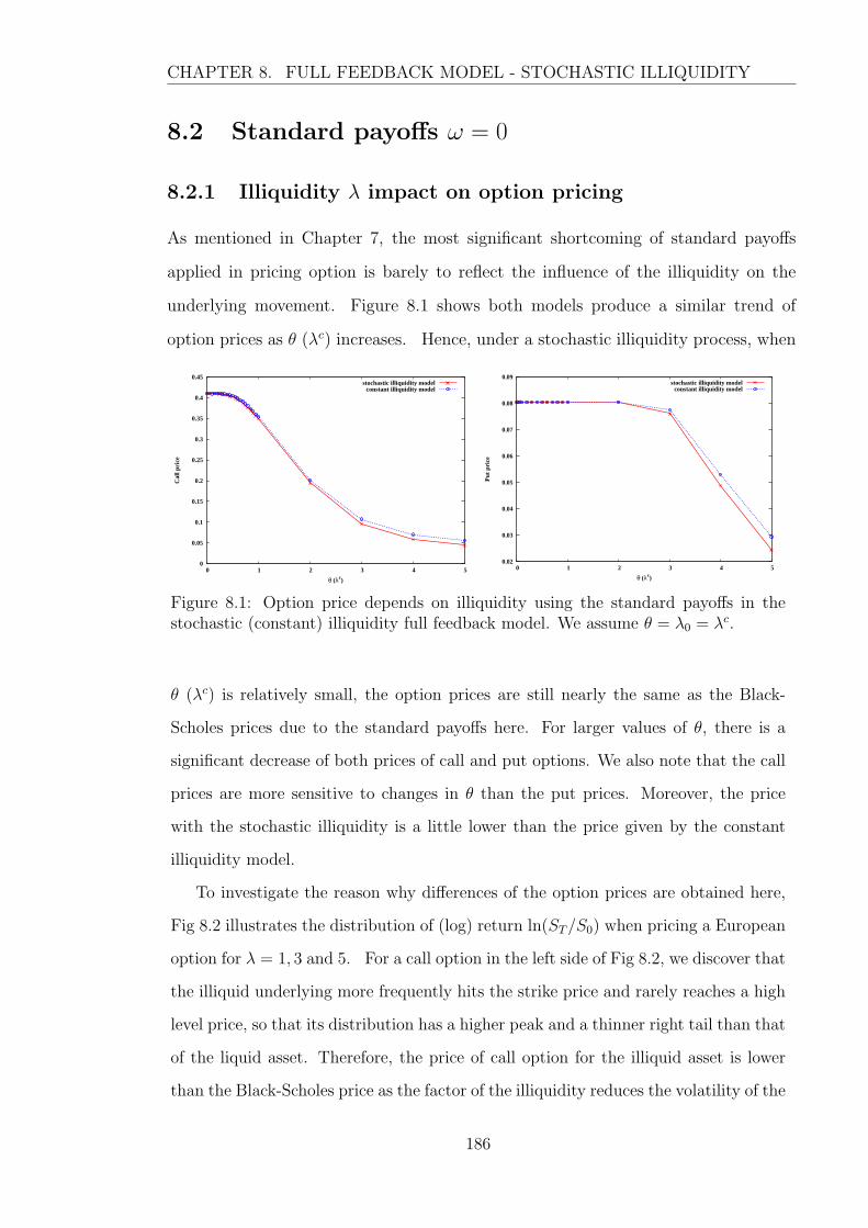
CHAPTER 8. FULL FEEDBACK MODEL - STOCHASTIC ILLIQUIDITY
8.2 Standard payoffs ω = 0
8.2.1 Illiquidity λ impact on option pricing
As mentioned in Chapter 7, the most significant shortcoming of standard payoffs
applied in pricing option is barely to reflect the influence of the illiquidity on the
underlying movement. Figure 8.1 shows both models produce a similar trend of
option prices as θ (λc) increases. Hence, under a stochastic illiquidity process, when
0
0.05
0.1
0.15
0.2
0.25
0.3
0.35
0.4
0.45
0 1 2 3 4 5
Cal
l pri
ce
θ (λc)
stochastic illiquidity modelconstant illiquidity model
0.02
0.03
0.04
0.05
0.06
0.07
0.08
0.09
0 1 2 3 4 5
Put
pri
ce
θ (λc)
stochastic illiquidity modelconstant illiquidity model
Figure 8.1: Option price depends on illiquidity using the standard payoffs in thestochastic (constant) illiquidity full feedback model. We assume θ = λ0 = λc.
θ (λc) is relatively small, the option prices are still nearly the same as the Black-
Scholes prices due to the standard payoffs here. For larger values of θ, there is a
significant decrease of both prices of call and put options. We also note that the call
prices are more sensitive to changes in θ than the put prices. Moreover, the price
with the stochastic illiquidity is a little lower than the price given by the constant
illiquidity model.
To investigate the reason why differences of the option prices are obtained here,
Fig 8.2 illustrates the distribution of (log) return ln(ST/S0) when pricing a European
option for λ = 1, 3 and 5. For a call option in the left side of Fig 8.2, we discover that
the illiquid underlying more frequently hits the strike price and rarely reaches a high
level price, so that its distribution has a higher peak and a thinner right tail than that
of the liquid asset. Therefore, the price of call option for the illiquid asset is lower
than the Black-Scholes price as the factor of the illiquidity reduces the volatility of the
186
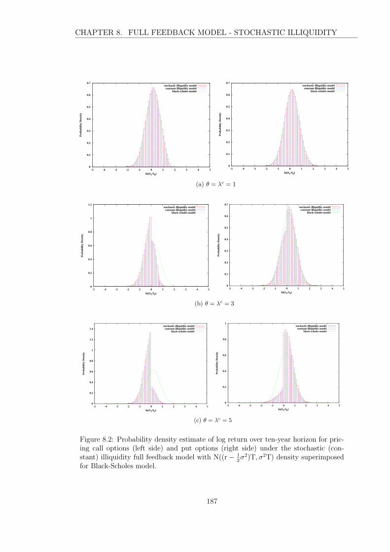
CHAPTER 8. FULL FEEDBACK MODEL - STOCHASTIC ILLIQUIDITY
0
0.1
0.2
0.3
0.4
0.5
0.6
0.7
-5 -4 -3 -2 -1 0 1 2 3 4 5
Pro
babi
lity
Den
sity
ln(ST/S0)
stochastic illiquidity modelconstant illiquidity model
black-scholes model
0
0.1
0.2
0.3
0.4
0.5
0.6
0.7
-5 -4 -3 -2 -1 0 1 2 3 4 5
Pro
babi
lity
Den
sity
ln(ST/S0)
stochastic illiquidity modelconstant illiquidity model
black-scholes model
(a) θ = λc = 1
0
0.2
0.4
0.6
0.8
1
1.2
-5 -4 -3 -2 -1 0 1 2 3 4 5
Pro
babi
lity
Den
sity
ln(ST/S0)
stochastic illiquidity modelconstant illiquidity model
black-scholes model
0
0.1
0.2
0.3
0.4
0.5
0.6
0.7
-5 -4 -3 -2 -1 0 1 2 3 4 5
Pro
babi
lity
Den
sity
ln(ST/S0)
stochastic illiquidity modelconstant illiquidity model
black-scholes model
(b) θ = λc = 3
0
0.2
0.4
0.6
0.8
1
1.2
1.4
-5 -4 -3 -2 -1 0 1 2 3 4 5
Pro
babi
lity
Den
sity
ln(ST/S0)
stochastic illiquidity modelconstant illiquidity model
black-scholes model
0
0.2
0.4
0.6
0.8
1
-5 -4 -3 -2 -1 0 1 2 3 4 5
Pro
babi
lity
Den
sity
ln(ST/S0)
stochastic illiquidity modelconstant illiquidity model
black-scholes model
(c) θ = λc = 5
Figure 8.2: Probability density estimate of log return over ten-year horizon for pric-ing call options (left side) and put options (right side) under the stochastic (con-stant) illiquidity full feedback model with N((r− 1
2σ2)T, σ2T) density superimposed
for Black-Scholes model.
187

CHAPTER 8. FULL FEEDBACK MODEL - STOCHASTIC ILLIQUIDITY
underlying. As θ increases, the histograms tend to move away from the Black-Scholes
curve and shift to the left, where the call option will expire out-of-the-money. Both
illiquidity models produce nearly the same distribution of log return, in particular
when θ = 3 and 5, the stochastic illiquidity model has a slightly higher peak which
results in a lower call price than that for the constant illiquidity model. For a put
option on the right side of Fig 8.2, there is a similar trend of underlying movements,
which is that the underlying potentially moves to a price region where the put option
will expire out-of-the-money. Nevertheless, the factor of illiquidity has less effect on
pricing a put option than a call option with the same value of θ, because the trend
is not felt until θ = 5 for the put option. This result is consistent with the price
reduction with respect to θ found in Fig 8.1.
θ = λ0 Abandonment Crossed Unconvergent Negative0 0(0) 0(0) 0(0) 0(0)0.05 0(0) 0(0) 0(0) 0(0)0.1 2(0) 0(0) 2(0) 0(0)0.3 150(0) 1(0) 50(0) 99(0)0.5 1635(0) 10(0) 349(0) 1278(0)0.7 6592(0) 67(0) 1377(0) 5151(0)1 25318(5) 397(0) 6567(5) 18391(0)3 420715(56222) 1.553e+ 04 2.266e+ 05 179969
(1700) (3.409e+ 04) (20670)5 558225(299950) 2.294e+ 04 3.438e+ 05 193334
(2.299e+ 04) (1.562e+ 05) (122174)
Table 8.2: The number of the abandoned paths in the full feedback model withstochastic λ. The data in parentheses stand for put options and others for calloptions.
We also give the corresponding data on the number of abandoned paths in Ta-
ble 8.2. Compared with the data presented in Table 7.5 for the constant illiquidity
model in Chapter 7, these suggest that the stochastic illiquidity leads to somewhat
more abandoned paths in the simulation, but its maximum abandonment rate is
around 55% when θ = 5, which is still in an acceptable range so that the algorithm
of option pricing is still useful. With regard to abandonment reasons, the main cause
here is that simulated paths fail to obtain a convergent option price. This can help to
explain why we obtain a thin right tail and normal left tail of histograms in Fig 8.2
188
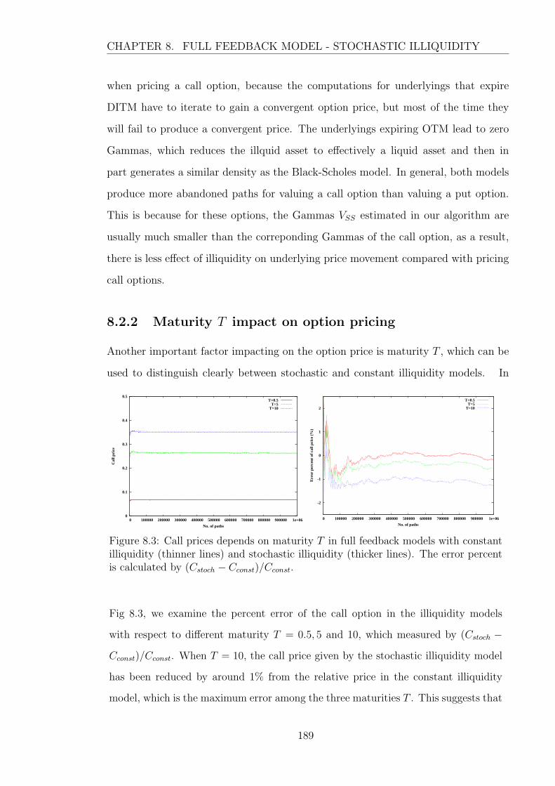
CHAPTER 8. FULL FEEDBACK MODEL - STOCHASTIC ILLIQUIDITY
when pricing a call option, because the computations for underlyings that expire
DITM have to iterate to gain a convergent option price, but most of the time they
will fail to produce a convergent price. The underlyings expiring OTM lead to zero
Gammas, which reduces the illquid asset to effectively a liquid asset and then in
part generates a similar density as the Black-Scholes model. In general, both models
produce more abandoned paths for valuing a call option than valuing a put option.
This is because for these options, the Gammas VSS estimated in our algorithm are
usually much smaller than the correponding Gammas of the call option, as a result,
there is less effect of illiquidity on underlying price movement compared with pricing
call options.
8.2.2 Maturity T impact on option pricing
Another important factor impacting on the option price is maturity T , which can be
used to distinguish clearly between stochastic and constant illiquidity models. In
0
0.1
0.2
0.3
0.4
0.5
0 100000 200000 300000 400000 500000 600000 700000 800000 900000 1e+06
Cal
l pri
ce
No. of paths
T=0.5T=5
T=10
-2
-1
0
1
2
0 100000 200000 300000 400000 500000 600000 700000 800000 900000 1e+06
Err
or p
erce
nt o
f ca
ll pr
ice
(%)
No. of paths
T=0.5T=5
T=10
Figure 8.3: Call prices depends on maturity T in full feedback models with constantilliquidity (thinner lines) and stochastic illiquidity (thicker lines). The error percentis calculated by (Cstoch − Cconst)/Cconst.
Fig 8.3, we examine the percent error of the call option in the illiquidity models
with respect to different maturity T = 0.5, 5 and 10, which measured by (Cstoch −Cconst)/Cconst. When T = 10, the call price given by the stochastic illiquidity model
has been reduced by around 1% from the relative price in the constant illiquidity
model, which is the maximum error among the three maturities T . This suggests that
189
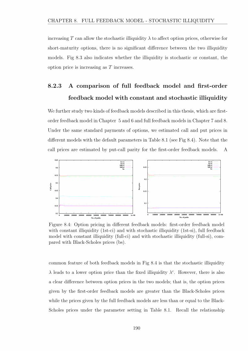
CHAPTER 8. FULL FEEDBACK MODEL - STOCHASTIC ILLIQUIDITY
increasing T can allow the stochastic illiquidity λ to affect option prices, otherwise for
short-maturity options, there is no significant difference between the two illiquidity
models. Fig 8.3 also indicates whether the illiquidity is stochastic or constant, the
option price is increasing as T increases.
8.2.3 A comparison of full feedback model and first-order
feedback model with constant and stochastic illiquidity
We further study two kinds of feedback models described in this thesis, which are first-
order feedback model in Chapter 5 and 6 and full feedback models in Chapter 7 and 8.
Under the same standard payments of options, we estimated call and put prices in
different models with the default parameters in Table 8.1 (see Fig 8.4). Note that the
call prices are estimated by put-call parity for the first-order feedback models. A
0.3
0.35
0.4
0.45
0.5
0.55
0.6
0.65
0 100000 200000 300000 400000 500000 600000 700000 800000 900000 1e+06
Cal
l pri
ce
No. of paths
1st-ci1st-si
full-cifull-si
bs
0.1
0.15
0.2
0.25
0 100000 200000 300000 400000 500000 600000 700000 800000 900000 1e+06
Put
pri
ce
No. of paths
1st-ci1st-si
full-cifull-si
bs
Figure 8.4: Option pricing in different feedback models: first-order feedback modelwith constant illiquidity (1st-ci) and with stochastic illiquidity (1st-si), full feedbackmodel with constant illiquidity (full-ci) and with stochastic illiquidity (full-si), com-pared with Black-Scholes prices (bs).
common feature of both feedback models in Fig 8.4 is that the stochastic illiquidity
λ leads to a lower option price than the fixed illiquidity λc. However, there is also
a clear difference between option prices in the two models; that is, the option prices
given by the first-order feedback models are greater than the Black-Scholes prices
while the prices given by the full feedback models are less than or equal to the Black-
Scholes prices under the parameter setting in Table 8.1. Recall the relationship
190
CHAPTER 8. FULL FEEDBACK MODEL - STOCHASTIC ILLIQUIDITY
between option prices and illiquidity λ in Fig 6.9 for the first-order feedback model,
i.e. the option price should increase beyond the Black-Scholes prices with λ first, then
afterwards it decreases with λ and might be lower than the Black-Scholes price. This
implies a problem with the application of the standard payoffs in the full feedback
model. With standard payment functions we cannot see such a increase with λ in
Fig 8.1, where the option prices estimated are shown to be close to the Black-Scholes
prices and lower than the Black-Scholes prices when illiquidity parameters chosen are
big enough, such as θ = λc > 1. Therefore, a smoothed payoff will be introduced and
discussed in the next section to complete our study of the full feedback problem.
8.3 Smoothing payoffs ω 6= 0
In this section, we focus on the smoothing function introduced in Section 7.2 where
ω = 0.1 and ω = 1, which represent a slightly smoothed payoff and a much smoothed
payoff, respectively. The impact of λ along nonzero ω on pricing European options
is illustrated and explored to investigate put-call parity. Moreover, we also analyze
implied volatilities calculated by Black-Scholes option pricing formula (see reference
in Wilmott, 2006) in the illiquidity models.
8.3.1 Illiquidity λ impact on pricing option
Fig 8.5 provides the results of option prices and the corresponding deviations from
put-call parity. It is clear that the option price estimated by the smoothed payoff
is more sensitive to small values of θ or λc than that of the price using a standard
payoff, which is similar to the Black-Scholes price in Fig 8.1. For both options,
there is a slight increase of option prices in θ, with a significant decline thereafter
in the stochastic illiquidity model, except for certain θ such as θ = 5 for pricing a
call option. Fig 8.5 also presents the corresponding option prices in the constant
illiquidity model, and shows that both illiquidity models produce similar values of
option price and deviation from put-call parity. We find that the full feedback model
with the smoothed payoff differs from that of the standard payoffs with large values
191

CHAPTER 8. FULL FEEDBACK MODEL - STOCHASTIC ILLIQUIDITY
0
0.1
0.2
0.3
0.4
0.5
0 1 2 3 4 5
Cal
l pri
ce
θ (λc)
ω=0.1
stochastic illiquidity modelconstant illiquidity model
0.1
0.15
0.2
0.25
0.3
0.35
0.4
0.45
0.5
0.55
0 1 2 3 4 5
Cal
l pri
ce
θ (λc)
ω=1.0
stochastic illiquidity modelconstant illiquidity model
0
0.02
0.04
0.06
0.08
0.1
0.12
0 1 2 3 4 5
Put
pri
ce
θ (λc)
stochastic illiquidity modelconstant illiquidity model
0
0.05
0.1
0.15
0.2
0.25
0.3
0 1 2 3 4 5
Put
pri
ce
θ (λc)
stochastic illiquidity modelconstant illiquidity model
-0.35
-0.3
-0.25
-0.2
-0.15
-0.1
-0.05
0
0.05
0.1
0 1 2 3 4 5
Dev
iati
on o
f P
CP
θ (λc)
stochastic illiquidity modelconstant illiquidity model
-0.4
-0.3
-0.2
-0.1
0
0.1
0 1 2 3 4 5
Dev
iati
on o
f P
CP
θ (λc)
stochastic illiquidity modelconstant illiquidity model
Figure 8.5: Option price depends on illiquidity in the stochastic (constant) illiquidityfull feedback model under smoothing payoffs. We also give the corresponding errorfrom put call parity assuming θ = λ0 = λc. The left panel is for ω = 0.1 and theright panel for ω = 1.0.
192

CHAPTER 8. FULL FEEDBACK MODEL - STOCHASTIC ILLIQUIDITY
of θ as there is no sign to conclude that the stochastic illiquidity leads to lower option
prices than the constant illiquidity. In particular, we find that larger values of θ would
cause abnormal behaviour of option prices, such as near zero prices or suddenly rising
prices. To investigate the behaviour, we provide the number of abandoned paths
from the relative simulations in Table 8.3. From Table 8.3, there are a significant
number of abandoned paths occurring in the simulation when θ is large, such as the
abandonment rate is around 99% at θ = 5. Therefore, a result from the simulations
cannot be used as a fair price of the option. This implies that when using a smoothed
payoff, we should take care to choose the values of θ and ω. In this example, it suggests
that to avoid high rates of abandonment in the simulation, we require that θ < 1 for
ω = 0.1 and θ < 0.5 for ω = 1. Fig 8.6 illustrate how the smoothing parameter ω
impacts on the distributions of log return ln(ST/S0) assuming θ = 1. Compared with
the case of ω = 0, there exist few paths with ln(ST/S0) ≈ 0 in the case of ω = 0.1,
i.e. the underlying rarely hits the strike price K = S0. This is also found in the case
of ω = 1. In particular, for pricing the call option, most of the simulated paths expire
out-of the money, i.e. ST < K, then the call price is estimated be extremely small.
8.3.2 Implied volatility in illiquidity models
As stated in Liu and Yong (2005), price impact leads to an endogenous stochastic
volatility, which is able to describe the ‘smile-pattern’ of the implied volatility ob-
tained in the real market. We illustrate the Black-Scholes implied volatility arising
from full feedback illiquidity models as well as the first-order feedback models shown
in Chapter 5. The illustration in Fig 8.7 takes a trial value of ω = 0.1, because a
slightly smoothed function close to the standard payoff should not vanish the com-
parability between the full feedback effect and the first-order feedback. Similarly,
we choose λc = 0.5 to ensure that the algorithm would not create a high percent-
age of abandoned paths in the simulation. Also, the example is based on pricing a
put option rather than a call option, because without capping the estimated price
of the put option is more accurate than that for the call option as mentioned in
193

CHAPTER 8. FULL FEEDBACK MODEL - STOCHASTIC ILLIQUIDITY
θA
ban
don
edC
ross
edU
nco
nve
rgen
tN
egat
ive
θA
ban
don
edC
ross
edU
nco
nve
rgen
tN
egat
ive
ω=
0 .1
ω=
1 .0
00
00
00
00
00
(0)
(0)
(0)
(0)
(0)
(0)
(0)
(0)
0.00
515
635
2262
3493
840.
0553
8998
353
13(1
2764
)(1
6)(5
830)
(692
1)(4
9)(2
)(0
)(4
7)0.
0121
247
3586
0712
608
0.1
2942
164
95
2889
9(1
7451
)(2
9)(7
740)
(968
3)(3
59)
(12)
(6)
(342
)0.
0235
998
601.
492e
+04
2102
30.
217
3798
5400
5216
9358
(295
89)
(61)
(1.2
97e+
04)
(165
71)
(461
0)(1
91)
(55)
(438
9)0.
0352
104
119
2.21
9e+
0429
819
0.3
4029
051.
762e
+04
151
3882
10(4
2961
)(1
15)
(1.8
32e+
04)
(245
44)
(215
92)
(136
8)(1
90)
(202
22)
0.04
6831
918
62.
917e
+04
3898
70.
459
0624
3.68
1e+
0429
755
9385
(567
15)
(187
)(2
.308
e+04
)(3
3473
)(6
0079
)(5
180)
(406
)(5
5157
)0.
0583
334
314
3.63
8e+
0446
702
0.5
6815
786.
101e
+04
499
6285
45(6
9168
)(3
41)
(2.6
72e+
04)
(421
67)
(120
972)
(1.4
46e+
04)
(591
)(1
0761
2)0.
113
8074
1330
5.96
4e+
0477
301
0.6
7308
918.
8e+
0494
865
3229
(112
747)
(145
2)(3
.054
e+04
)(8
0972
)(1
9832
2)(3
.07e
+04
)(6
46)
(170
389)
0.3
2359
371.
503e
+04
5.57
7e+
0416
6831
0.7
7658
461.
122e
+05
1522
6658
71(1
6211
2)(1
.674
e+04
)(8
143)
(139
313)
(285
370)
(5.2
45e+
04)
(676
)(2
3741
6)0.
532
8740
3.81
2e+
045.
438e
+04
2400
590.
879
3913
1.28
1e+
0523
2367
8729
(198
744)
(4.3
55e+
04)
(1.5
31e+
04)
(144
548)
(375
293)
(8.1
41e+
04)
(585
)(3
0048
2)0.
745
8295
6.39
7e+
045.
508e
+04
3457
020.
981
6912
1.36
6e+
0529
7669
3544
(236
266)
(6.8
e+04
)(3
.373
e+04
)(1
4092
8)(4
6183
8)(1
.194
e+05
)(6
23)
(351
053)
1.0
6620
581.
044e
+05
5.74
8e+
0451
0484
1.0
8362
511.
39e+
0534
9171
0105
(298
953)
(9.9
54e+
04)
(6.1
4e+
04)
(145
548)
(540
519)
(1.6
88e+
05)
(592
)(3
8275
1)3.
081
5877
1.84
1e+
057.
598e
+04
5696
253.
097
0848
1.16
1e+
0517
2986
5765
(600
430)
(2.4
98e+
05)
(1.3
65e+
05)
(222
848)
(967
806)
(4.1
44e+
05)
(1.0
69e+
04)
(560
194)
5.0
8447
542.
033e
+05
7.09
5e+
0458
3214
5.0
9530
358.
191e
+04
3.12
8e+
0484
7145
(636
092)
(2.7
71e+
05)
(1.3
56e+
05)
(232
017)
(989
322)
(4.2
98e+
05)
(1.9
35e+
04)
(557
518)
Tab
le8.
3:T
he
num
ber
ofth
eab
andon
edpat
hs
for
Euro
pea
nop
tion
sin
106
sam
ple
pat
hs.
The
dat
ain
par
enth
eses
stan
dfo
rput
opti
ons
and
other
sfo
rca
llop
tion
s.
194
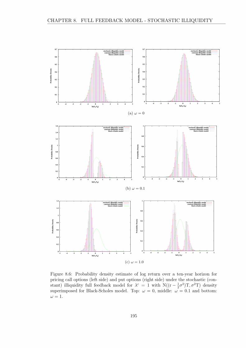
CHAPTER 8. FULL FEEDBACK MODEL - STOCHASTIC ILLIQUIDITY
0
0.1
0.2
0.3
0.4
0.5
0.6
0.7
-5 -4 -3 -2 -1 0 1 2 3 4 5
Pro
babi
lity
Den
sity
ln(ST/S0)
stochastic illiquidity modelconstant illiquidity model
black-scholes model
0
0.1
0.2
0.3
0.4
0.5
0.6
0.7
-5 -4 -3 -2 -1 0 1 2 3 4 5
Pro
babi
lity
Den
sity
ln(ST/S0)
stochastic illiquidity modelconstant illiquidity model
black-scholes model
(a) ω = 0
0
0.2
0.4
0.6
0.8
1
1.2
1.4
1.6
-5 -4 -3 -2 -1 0 1 2 3 4 5
Pro
babi
lity
Den
sity
ln(ST/S0)
stochastic illiquidity modelconstant illiquidity model
black-scholes model
0
0.2
0.4
0.6
0.8
1
-5 -4 -3 -2 -1 0 1 2 3 4 5
Pro
babi
lity
Den
sity
ln(ST/S0)
stochastic illiquidity modelconstant illiquidity model
black-scholes model
(b) ω = 0.1
0
0.2
0.4
0.6
0.8
1
1.2
1.4
-5 -4 -3 -2 -1 0 1 2 3 4 5
Pro
babi
lity
Den
sity
ln(ST/S0)
stochastic illiquidity modelconstant illiquidity model
black-scholes model
0
0.2
0.4
0.6
0.8
1
-5 -4 -3 -2 -1 0 1 2 3 4 5
Pro
babi
lity
Den
sity
ln(ST/S0)
stochastic illiquidity modelconstant illiquidity model
black-scholes model
(c) ω = 1.0
Figure 8.6: Probability density estimate of log return over a ten-year horizon forpricing call options (left side) and put options (right side) under the stochastic (con-stant) illiquidity full feedback model for λc = 1 with N((r− 1
2σ2)T, σ2T) density
superimposed for Black-Scholes model. Top: ω = 0, middle: ω = 0.1 and bottom:ω = 1.
195
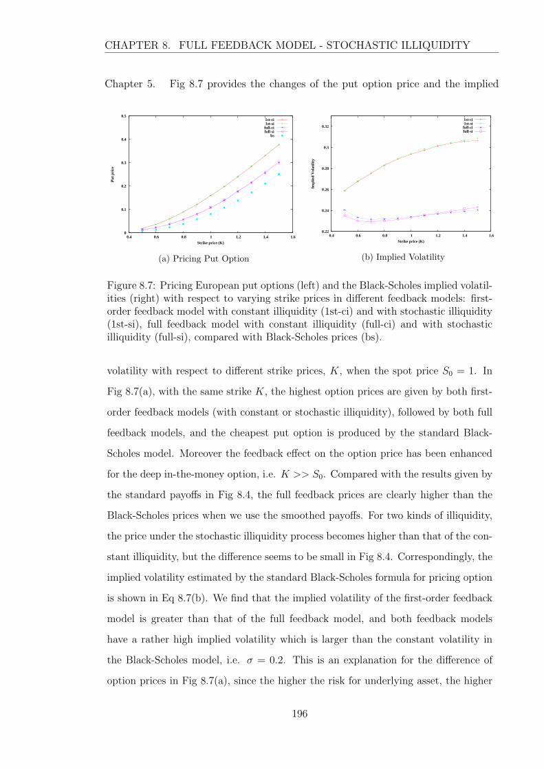
CHAPTER 8. FULL FEEDBACK MODEL - STOCHASTIC ILLIQUIDITY
Chapter 5. Fig 8.7 provides the changes of the put option price and the implied
0
0.1
0.2
0.3
0.4
0.5
0.4 0.6 0.8 1 1.2 1.4 1.6
Put
pri
ce
Strike price (K)
1st-ci1st-si
full-cifull-si
bs
(a) Pricing Put Option
0.22
0.24
0.26
0.28
0.3
0.32
0.4 0.6 0.8 1 1.2 1.4 1.6
Impl
ied
Vol
atili
ty
Strike price (K)
1st-ci1st-si
full-cifull-si
(b) Implied Volatility
Figure 8.7: Pricing European put options (left) and the Black-Scholes implied volatil-ities (right) with respect to varying strike prices in different feedback models: first-order feedback model with constant illiquidity (1st-ci) and with stochastic illiquidity(1st-si), full feedback model with constant illiquidity (full-ci) and with stochasticilliquidity (full-si), compared with Black-Scholes prices (bs).
volatility with respect to different strike prices, K, when the spot price S0 = 1. In
Fig 8.7(a), with the same strike K, the highest option prices are given by both first-
order feedback models (with constant or stochastic illiquidity), followed by both full
feedback models, and the cheapest put option is produced by the standard Black-
Scholes model. Moreover the feedback effect on the option price has been enhanced
for the deep in-the-money option, i.e. K >> S0. Compared with the results given by
the standard payoffs in Fig 8.4, the full feedback prices are clearly higher than the
Black-Scholes prices when we use the smoothed payoffs. For two kinds of illiquidity,
the price under the stochastic illiquidity process becomes higher than that of the con-
stant illiquidity, but the difference seems to be small in Fig 8.4. Correspondingly, the
implied volatility estimated by the standard Black-Scholes formula for pricing option
is shown in Eq 8.7(b). We find that the implied volatility of the first-order feedback
model is greater than that of the full feedback model, and both feedback models
have a rather high implied volatility which is larger than the constant volatility in
the Black-Scholes model, i.e. σ = 0.2. This is an explanation for the difference of
option prices in Fig 8.7(a), since the higher the risk for underlying asset, the higher
196

CHAPTER 8. FULL FEEDBACK MODEL - STOCHASTIC ILLIQUIDITY
the option price. The implied volatility in the first-order feedback models increases
when the option tends to be in-the-money, while the implied volatility given by the
full feedback models looks more like a skewed smile, which means a relatively high
volatility is also obtained for deep out-of-the-money options. In addition, stochastic
illiquidity is shown to have more impact on the implied volatility in the full feedback
models than the first-order feedback models. That is, the model with the stochastic
illiquidity provides a more skewed smile, where the increase of the volatility for deep
in-the-money options is found to be more pronounced than the increase for the deep
out-of-the-money. Therefore, the full feedback model with a stochastic illiquidity is
to be considered a more accurate model to capture the famous important feature of
the smile and skew volatility.
In summary, the numerical pricing option in the full feedback model is much more
complicated than in the first-order feedback model. Following our analysis above, it
turns out that the smoothed payoff is able to value the option price for small values of
the illiquidity θ or λc. However, there exists the difficulty of evaluating the price when
θ is relatively large because in such cases, the smoothing parameter, ω, accompanied
with the illiquidity, θ, could cause a number of abandoned paths and eventually
damage the simulation. Therefore, instead of the smoothed payoffs, for a severe
illiquidity situation, such as θ > 1, we recommend the use of a standard payoff to
price options, which is shown to have a better performance in the option valuation.
Besides the option pricing, we also explore that the Black-Scholes implied volatility
in the feedback models. With a proper setting of parameters θ and ω, the results
support that proposition that the full feedback model with stochastic illiquidity can
be regarded as better than other models in capturing the smile pattern of implied
volatility.
197
Chapter 9
Conclusions
... derivatives are financial weapons of mass destruction, carrying
dangers that, while now latent, are potentially lethal.
– Warren Buffett, Chairman of Berkshire Hathaway,
in the 2002 “Chairman’s Letter” to shareholders
9.1 Summaries
In this thesis, we have investigated applications of Monte Carlo methods to price
financial derivatives under practical models: jump diffusion models and illiquid asset
models with a feedback effect from large trades in markets.
For the jump diffusion processes introduced by Merton (1973), we develop a
simulation-based algorithm for pricing European options and Bermudan options.
There have been three modified jump diffusion models proposed in Chapter 3: multi-
dimensional jump models, one-dimensional jump models with stochastic volatility
and multi-dimensional jump models with stochastic volatility. To extend solution
to multi-dimensional option pricing problems, there is a difficulty in calculating the
correlation matrix for different underlying assets. The correlation in jump diffusion
models is shown be more complicated than in standard Black-Scholes models, because
we have to consider correlations not only for diffusion terms but also for jump terms
with regard to jump size and jump frequency. Following Clift (2007), we assume that
198
CHAPTER 9. CONCLUSIONS
the number of jumps is the sum of two independent Poisson random numbers, where
one is individual to the specific asset and the other is common, shared by all assets.
The jump size is determined by a multinormal distribution. Furthermore, we explore
the two factor jump diffusion asset model with correlated stochastic volatility that
follows a mean reverting jump diffusion process. Correlation is considered for differ-
ent assets and the different volatilities of the relative assets on two aspects: diffusion
term and jump term. The two-factor model requires roughly a doubling of compu-
tation cost to simulate the asset process compared with the one-factor model. The
rate of increase in costs is linearly with the number of dimensions, which is slower
than the rate of other numerical methods for high dimensional pricing problems (see
Hull, 2009).
In Chapter 3 we focus on the analysis of pricing Bermudan options using the
least-squares Monte-Carlo method proposed by Longstaff and Schwartz (2001). The
method has been improved to achieve enhanced accurate results with an extrapolation
process (see Duck et al., 2005). Through the results presented in Chapter 3, we
conclude that a proper set of the number of sample paths is particularly important
to correctly calculate Bermudan option prices when the extrapolation technique is
employed. The convenient choice as suggested by Duck et al. (2005) is to set the
number of sample paths as M = 2000, 4000 and 8000 respectively for the least-
squares regression, which implies that the option prices calculated by these three
samples are accurate. Furthermore, our results show that the extrapolation method
should be recommended to deal with pricing Bermudan option with a number of
exercise opportunities, which produces a more correct option price.
From Chapter 4 to Chapter 8, another kind of practical model is studied here
to realize the feedback trading which has a price impact on underlying assets. Our
feedback models are derived mainly from Glover (2008) and we also provide an ex-
tended version of feedback model with undetermined volatility. For first-order feed-
back model in Chapter 5 and Chapter 6, the implementation of Monte Carlo is quite
straightforward using the exact value of the second derivative of options with respect
to stock prices from the Black-Scholes formula. There exists a potential problem
199

CHAPTER 9. CONCLUSIONS
underlying asset price simulation for this model, which is production of (financially
unreal) negative prices of the asset. We analyze the cause of the occurrence of neg-
ative prices and find the ‘dangerous’ area with respect to stock prices S and time to
maturity τ , where the following price S(τ −∆t) simulated by S(τ) is usually nega-
tive, assuming ∆t is the size of timesteps used in the simulation. Our suggestion for
these negative prices is to interrupt the particular path and to start simulating the
next sample path. When the volatility follows a stochastic process, the asset price
tends to be more volatile, leading to more negative prices occurring the simulation.
It is important to subtract the number of negative paths from the total sample paths
when calculating the expected value of option price.
For full feedback models in Chapter 7 and Chapter 8, we suggest estimating the
second derivative (i.e. Gamma) using a three-point difference method. In order to
apply this method, three sample paths are required, starting with a slightly different
stock price, but simulating with the same set of random numbers for each timestep.
We also need some additional conditions on the numerical method: the three sample
paths cannot cross at each time point, otherwise the method fails; the resulting
option price from the iteration process is shown to be convergent; the estimate of
asset prices is strictly positive. We have to abandon sample paths that violate these
necessary conditions. Assuming the law of large number still holds here, then the
option price can be computed from the live simulated paths. However, the total
number of abandoned paths should be noted and high levels of abandonment rate
avoided via a proper set of parameters. A smoothed payoff function for European
options has an advantage over the standard payoffs because it can realize more non-
zero values of Gammas to reflect the price impact. We present the results of the
standard payoffs and smoothing payoffs in the case of full feedback models. When
considering a stochastic volatility process, the option price is shown to be slightly
different from the price with the constant volatility.
There is another finding in these feedback models, which is the use of put-call
parity. Our results show that the model is more suitable to price put options than call
options, because some simulated asset prices can be extremely large when evaluating
200

CHAPTER 9. CONCLUSIONS
a convergent price for call options.
9.2 Further research
Further research could study the illiquid asset model with jumps. The basic illiquid-
ity model is able to capture price changes according to trading volume in the market,
while the jump diffusion model is used to explain price movements as partly responsi-
ble for unexpected market crashes (irrelevant to the trading itself). Combining these
two kinds of models, one might obtain a more reasonable model to capture realistic
price movement in a stock market. Incorporating a stochastic volatility and/or a
stochastic interest rate is another possible direction to complete our model. It is im-
portant to investigate the correlations between these state variables in the extended
model, meanwhile the extended model may involve more computational difficulties
in multi-dimensional framework.
Monte Carlo has been shown to be a feasible tool for pricing complex options in
the more complex (and, we trust, more realistic) environment beyond Black-Scholes-
Merton described in this thesis, such as Bermudan options, exotic options and multi-
asset options. The Bermudan options priced using a LSM algorithm can still be
evaluated in the illiquid model with jumps. Monte Carlo valuation for exotic options:
barrier options, Asian options and Parisian/ParAsian option (see Xiao, 2007), has
a significant advantage in terms of ease of implementation over most other numer-
ical methods; the extension to options with other more exotic boundary conditions
should follow naturally. One could then use the Monte Carlo method to mimic the
behaviour of these exotic options in the feedback model with jumps. These options
can be straightforwardly extended to multi-asset options, whose valuation is gener-
ally required less computational cost using the Monte Carlo methods as its O(1/√n)
convergence rate holds for all dimensions.
Alternatively, we can also pay attention to the efficiency of Monte Carlo estima-
tors, in particular, for pricing complex options. Several basic and popular variance
reduction techniques and discretization have been introduced in Chapter 2. We can
201

CHAPTER 9. CONCLUSIONS
adopt these technologies to improve the Monte Carlo simulation for more sensible
feedback models.
We have neglected calibration of the asset models presented in this thesis, which
is an interesting area to investigate how to estimate these models using market data.
The importance of different variables (e.g. illiquidity lambda, jump size, jump fre-
quency, etc.) will be explored through these empirical test.
202

Appendix A
Basic Notation and Abbreviation
We adopt the following notation and abbreviations throughout the thesis.
Symbol DescriptionP (real-world) probability measureQ (risk-neutral) probability measure:= defined as or denoted byx> transpose of the vector x∼ with distributionE expectation operatorV ar variance operatorCov covariance operatorlog natural logarithmN(µ, σ2) Normal distribution with mean µ and variance σ2
Poisson(λ) Poisson distribution with mean λGamma(k, λ) Gamma distribution with mean kλ and varaince kλ2
(a, b) the open interval a < x < b[a, b] the closed interval a ≤ x ≤ bf ′ the first derivative of a function ff ′′ the second derivative of a function ff (i) the ith derivative of a function f∂if∂xi the ith order partial derivative of a function f with respect to xO(n−m) the approximation error is of order less than n−m
(the order of magnitude of n−m)
Table A.1: Mathematical Symbols
203

APPENDIX A. BASIC NOTATION AND ABBREVIATION
Symbol Descriptionr riskless interest rateσ volatility parameter of the stockW Wiener process (Brownian motion)τ time to maturityt current timeT maturity timeSt underlying price at time tK strike price
Table A.2: Elements of options
Abbreviations Descriptiona.s. almost surelyi.i.d. independent and identical distributedw.r.t. with respect tor.v. random variableCIR Cox Ingersoll Ross modelMC Monte CarloPDE Partial Differential EquationQMC Quasi Monte CarloSDE Stochastic Differential Equation
Table A.3: Abbreviations
204

Appendix B
Computational Time for 1D-MJD
Models
Number of Number of N = 5 N = 50 N = 100 N = 300sample paths runs
1000 5000 27.57 61.63 103.45 314.6210000 62.87 131.45 216.42 640.32
2000 5000 63.10 133.92 219.28 654.6010000 125.63 273.67 446.65 1312.33
4000 5000 134.27 275.78 467.68 1366.6710000 275.95 557.68 937.18 2703.33
6000 5000 206.82 425.22 719.78 2068.3510000 420.17 856.37 1425.00 4146.62
Table B.1: The total computational time (minutes) required for 1D-MJD models.The parameters employed are the same as those in Fig 3.5
205

References
Abramowitz, M. and Stegun, I. (1972), Handbook of mathematical functions with
formulas, graphs, and mathematical tables, Courier Dover Publications.
Amin, K. and Ng, V. (1993), ‘Option valuation with systematic stochastic volatility’,
The Journal of Finance 48(3), 881–910.
Andersen, L. (2000), ‘A simple approach to the pricing of Bermudan swaptions in the
multi-factor LIBOR market model’, Journal of Computational Finance 3(2), 5–
32.
Andersen, L. and Andreasen, J. (2000), ‘Jump-diffusion processes: volatility smile
fitting and numerical methods for option pricing’, Review of Derivatives Research
4, 231–262.
Andersen, L. and Broadie, M. (2004), ‘Primal-dual simulation algorithm for pricing
multidimensional American options’, Management Science 50(9), 1222–1234.
Andersen, T., Bollerslev, T., Diebold, F. and Labys, P. (2001), ‘The distribution of
realized exchange rate volatility’, Journal of the American Statistical Association
96(453), 42–55.
Bakshi, G., Cao, C. and Chen, Z. (1997), ‘Empirical performance of alternative option
pricing models’, The Journal of Finance 53(5), 2003–2049.
Bakstein, D. and Howison, S. (2003), ‘A non-arbitrage liquidity model with observable
parameters’, Mathematical Finance .
206
REFERENCES
Ball, C. and Torous, W. (1985), ‘On jumps in common stock prices and their impact
on call option pricing’, The Journal of Finance 40(1), 155–173.
Bally, V., Pages, G. and Printems, J. (2002), ‘First-order schemes in the numerical
quantization method’, Mathematical Finance 13(1), 1–16.
Bally, V., Pages, G. and Printems, J. (2005), ‘A quantization method for pricing
and hedging multi-dimensional American style options’, Mathematical Finance
15(1), 119–168.
Bank, P. and Baum, D. (2004), ‘Hedging and portfolio optimization in financial
markets with a large trader’, Mathematical Finance 14(1), 1–18.
Barraquand, J. and Martineau, D. (1995), ‘Numerical valuation of high dimensional
multivariate American securities’, The Journal of Financial and Quantitative
Analysis 30(3), 383–405.
Bates, D. (1996), ‘Jumps and stochastic volatility: exchange rate processes implicit
in deutsche mark options’, The Review of Financial Studies 9(1), 69–107.
Benhamou, E. (2002), ‘Smart Monte Carlo: various tricks using Malliavin calculus’,
Quantitative Finance 2(5), 329–336.
Birge, J. (1995), Quasi-Monte Carlo approaches to option pricing, Technical re-
port 94-19, Department of Industrial and Operations Engineering, University
of Michigan, Ann Arbor, MI 48109.
Black, F. and Scholes, M. (1973), ‘The pricing of options and corporate liabilities’,
The Journal of Political Economy 81(3), 637–654.
Bolia, N. and Juneja, S. (2005), ‘Monte Carlo methods for pricing financial options’,
Sadhana 30(2&3), 347–385.
Bossaerts, P. (1989), ‘Simulation estimators of optimal early exercise’, working paper,
Carnegie Mellon University, Pittsburgh, PA .
207
REFERENCES
Box, G. and Muller, M. (1958), ‘A note on the generation of random normal deviates’,
The Annals of Mathematical Statistics 29(2), 610–611.
Boyle, P. (1977), ‘Options: a Monte Carlo approach’, Journal of Financial Economics
4(3), 323–338.
Boyle, P., Broadie, M. and Glasserman, P. (1997), ‘Monte Carlo methods for security
pricing’, Journal of Economic Dynamics and Control 21, 1267–1321.
Bratley, P., Fox, B. and Schrage, L. (1987), A guide to simulation, 2nd edn, Springer-
Verlag, New York.
Broadie, M. and Glasserman, P. (1996), ‘Estimating security price derivatives using
simulation’, Management Science 42(2), 269–285.
Broadie, M. and Glasserman, P. (1997), ‘Pricing American-style securities using sim-
ulation’, Journal of Economic Dynamics and Control 21(8-9), 1323–1352.
Broadie, M. and Glasserman, P. (2004), ‘A stochastic mesh method for pricing high-
dimensional American options’, Journal of Computational Finance 7(4), 35–72.
Carr, P. and Yang, G. (2001), Simulating Bermudan interest rate derivatives, in
M. Avellaneda, ed., ‘Quantitative Analysis in Financial Markets: collected pa-
pers of the New York University Mathematical Finance Seminar’, Vol. 2, World
Scientific, pp. 295–316.
Carriere, J. (1996), ‘Valuation of the early-exercise price for options using simula-
tions and nonparametric regression’, Insurance: Mathematics and Economics
19(1), 19–30.
Cerrato, M. and Cheung, K. (2007), Valuing American style options by least squares
method, Money Macro and Finance (MMF) Research Group Conference 2006 49,
Money Macro and Finance Research Group.
Cetin, U., Jarrow, R. and Protter, P. (2004), ‘Liquidity risk and arbitrage pricing
theory’, Finance and Stochastics 8(3), 311–342.
208
REFERENCES
Cetin, U., Jarrow, R., Protter, P. and Warachka, M. (2006), ‘Pricing options in an
extended Black Scholes economy with illiquidity: theory and empirical evidence’,
The Review of Financial Studies 19(2), 493–529.
Cetin, U. and Rogers, L. (2006), ‘Modeling liquidity effects in discrete time’, Mathe-
matical Finance 17(1), 15–29.
Chan, W. (2003), ‘A correlated bivariate Poisson jump model for foreign exchange’,
Empirical Economics 28(4), 669–686.
Clement, E., Lamberton, D. and Protter, P. (2002), ‘An analysis of a least
squares regression method for American option pricing’, Finance and Stochastics
6(4), 449–472.
Clewlow, L. and Strickland, C. (1998), Pricing interest rate exotics by Monte Carlo
simulation, in B. Dupire, ed., ‘Monte Carlo: Methodologies and Applications for
Pricing and Risk Management’, Risk Publications, London, chapter 17.
Clift, S. (2007), Linear and non-linear monotone methods for valuing financial options
under two-factor, jump-diffusion models, PhD thesis, University of Waterloo.
Cox, J., Ingersoll, J. and Ross, S. (1985), ‘A theory of the term structure of interest
rates’, Econometrica 53(2), 385–407.
Cox, J. and Ross, S. (1976), ‘The valuation of options for alternative stochastic
processes’, Journal of Financial Economics 3(1-2), 145–166.
Cuoco, D. and Cvitanic, J. (1998), ‘Optimal consumption choices for a ‘large’ in-
vestor’, Journal of Economic Dynamics and Control 22(3), 401–436.
Cvitanic, J. and Ma, J. (1996), ‘Hedging options for a large investor and forward-
backward SDEs’, The Annals of Applied Probability 6, 370–398.
Duck, P., Newton, D., Widdicks, M. and Leung, Y. (2005), ‘Enhancing the accuracy
of pricing American and Bermudan options’, Journal of Derivatives 12(4), 34–
44.
209

REFERENCES
Duffie, D. and Glynn, P. (1995), ‘Efficient Monte Carlo simulation of security prices’,
The Annals of Applied Probability 5(4), 897–905.
Duffie, D., Pan, J. and Singleton, K. (2000), ‘Transform analysis and asset pricing
for affine jump-diffusions’, Econometrica 68(6), 1343–1376.
Duffy, D. (2008), ‘Numerical analysis of jump diffusion models: a partial differential
equation approach’, Datasim Financial Website .
*http://www.datasimfinancial.com/UserFiles/articles/PIDE.pdf
El-Borai, M., El-Nadi, K., Mostafa, O. and Ahmed, H. (2005), ‘Numerical methods
for some nonlinear stochastic differential equations’, Applied Mathematics and
Computation 168(1), 65–75.
Eraker, B., Johannes, M. and Polson, N. (2003), ‘The impact of jumps in volatility
and returns’, The Journal of Finance 58(3), 1269–1300.
Esser, A. and Monch, B. (2002), ‘Modeling feedback effects with stochastic liquidity’,
SSRN eLibrary .
Feller, W. (1951), ‘Two singular diffusion problems’, The Annals of Mathematics
54(1), 173–182.
Fournie, E., Lasry, J., Lebuchoux, J. and Lions, P. (2001), ‘Applications of Malli-
avin calculus to Monte-Carlo methods in Finance II’, Finance and Stochastics
5(2), 201–236.
Fournie, E., Lasry, J., Lebuchoux, J., Lions, P. and Touzi, N. (1999), ‘Applications of
Malliavin calculus to Monte Carlo methods in finance’, Finance and Stochastics
3, 391–412.
Frey, R. (1996), ‘The pricing and hedging of options in finitely elastic markets’, SSRN
eLibrary .
210

REFERENCES
Frey, R. (2000), Market illiquidity as a source of model risk in dynamic hedging, in
R. Gibson, ed., ‘Model risk: concepts, calibration and pricing’, Risk Publication,
London, pp. 125–136.
Frey, R. and Patie, P. (2002), Risk management for derivatives in illiquid markets:
a simulation study, in K. Sandmann, P. Schonbucher and D. Sondermann, eds,
‘Advances in finance and stochastics: essays in honour of Dieter Sondermann’,
Springer, pp. 137–159.
Frey, R. and Stremme, A. (1997), ‘Market volatility and feedback effects from dy-
namic hedging’, Mathematical Finance 7(4), 351–374.
Garcia, D. (2003), ‘Convergence and biases of Monte Carlo estimates of American
option prices using a parametric exercise rule’, Journal of Economic Dynamics
and Control 27(10), 1855–1879.
Glasserman, P. (2003), Monte Carlo Methods in Financial Engineering, Springer.
Glasserman, P., Heidelberger, P. and Shahabuddin, P. (1999), ‘Asymptotically opti-
mal importance sampling and stratification for pricing path-dependent options’,
Mathematical Finance 9(2), 117–152.
Glasserman, P. and Yu, B. (2004), ‘Number of paths versus number of basis functions
in American option pricing’, The Annals of Applied Probability 14(4), 2090–2119.
Glover, K. (2008), The analysis of PDEs arising in nonlinear and non-standard option
pricing, PhD thesis, University of Manchester.
Guasoni, P. and Robertson, S. (2008), ‘Optimal importance sampling with explicit
formulas in continuous time’, Finance and Stochastics 12(1), 1–19.
Halton, J. (1960), ‘On the efficiency of certain quasi-random sequences of points in
evaluating multi-dimensional integrals’, Numerische Mathematik 2(1), 84–90.
Haugh, M. and Kogan, L. (2004), ‘Pricing American options: a duality approach’,
Operations Research 52(2), 258–270.
211

REFERENCES
Heston, S. (1993), ‘A closed-form solution for options with stochastic volatility with
applications to bond and currency options’, The Review of Financial Studies
6(2), 327–343.
Higham, D. (2001), ‘An algorithmic introduction to numerical simulation of stochastic
differential equations’, SIAM Review 43(3), 525–546.
Higham, D. (2004), An introduction to financial option valuation: mathematics,
stochastics and computation, Cambridge University Press.
Higham, D. and Mao, X. (2005), ‘Convergence of Monte Carlo simulations involv-
ing the mean-reverting square root process’, Journal of Computational Finance
8(3), 35–62.
Huang, X. and Tauchen, G. (2005), ‘The relative contribution of jumps to total price
variance’, Journal of Financial Econometrics 3(4), 456–499.
Hull, J. (2009), Options, futures, and other derivatives, 7th edn, Pearson Prentice
Hall.
Hull, J. and White, A. (1987), ‘The pricing of options on assets with stochastic
volatilities’, The Journal of Finance 42(2), 281–300.
Ito, K. (1951), ‘On stochastic differential equations’, Memoirs of the American Math-
ematical Society 4.
Jarrow, R. (1992), ‘Market manipulation, bubbles, corners and short squeezes’, The
Journal of Financial and Quantitative Analysis 27(3), 311–336.
Jarrow, R. (1994), ‘Derivative securities markets, market manipulation and option
pricing theory’, The Journal of Financial and Quantitative Analysis 29(2), 241–
261.
Jarrow, R. and Rosenfeld, E. (1984), ‘Jump risks and the intertemporal capital asset
pricing model’, The Journal of Business 57(3), 337–351.
212
REFERENCES
Jensen, M. and Svenstrup, M. (2005), ‘Efficient control variates and strategies for
Bermudan swaptions in a Libor market model’, Journal of Derivatives 12(4), 20–
33.
Jorion, P. (1988), ‘On jump processes in the foreign exchange and stock markets’,
The Review of Financial Studies 1(4), 427–445.
Joy, C., Boyle, P. and Tan, K. (1996), ‘Quasi-Monte Carlo methods in numerical
finance’, Management Science 42(6), 926–938.
Kloeden, P. and Platen, E. (1999), Numerical solution of stochastic differential equa-
tion, Springer.
Kou, S. (2002), ‘A jump-diffusion model for option pricing’, Management Science
48(8).
Kwok, Y. (2008), Mathematical models of financial derivatives, Springer.
Law, A. and Kelton, W. (1991), Simulation modeling and analysis, 2nd edn, McGraw-
Hill, New York.
Lehmer, D. (1951), Mathematical methods in large-scale computing units, in ‘Pro-
ceedings of the 2nd Symposium on Large-Scale Digital Calculating Machinery’,
Cambridge, MA: Harvard University Press, pp. 141–146.
Lewis, A. (2001), ‘A simple option formula for general jump-diffusion and other
exponential Levy processes’, SSRN eLibrary .
Liao, H., Chen, T. and Chou, T. (2005), ‘Multi-period corporate short-term credit
risk assessment— a state-dependent stochastic liquidity balance model’, SSRN
eLibrary .
Liu, B. (2009), Extensions on defaultable bond valuation with Parasian and nonlin-
earity features, PhD thesis, University of Manchester.
Liu, H. and Yong, J. (2005), ‘Option pricing with an illiquid underlying asset market’,
Journal of Economic Dynamics and Control 29(12), 2125–2156.
213

REFERENCES
London, J. (2004), Modeling derivatives in C++, John Wiley and Sons.
Longstaff, F. and Schwartz, E. (2001), ‘Valuing American options by simulation: a
simple least-squares approach’, The Review of Financial Studies 14(1), 113–147.
Martzoukos, S. (2003), ‘Contingent claims on foreign assets following jump-diffusion
processes’, Review of Derivatives Research 6(1), 27–45.
Matei, S. (2005), A multivariate jump-diffusion model and pricing of multi-currency
options, Master’s thesis, University of Zurich.
Matsuda, K. (2004), ‘Introduction to Merton jump diffusion model’, working paper .
Merton, R. (1973), ‘The theory of rational option pricing’, The Bell Journal of Eco-
nomics and Management Science 4(1), 141–183.
Merton, R. (1976), ‘Option pricing when underlying stock returns are discontinuous’,
Journal of Financial Economics 3(1-2), 125–144.
Miller, I. and Miller, M. (2004), John E. Freund’s mathematical statistics with appli-
cations, 7th edn, Pearson Prentice Hall.
Milstein, G. (1975), ‘Approximate integration of stochastic differential equations’,
Theory of Probability and its Applications 19(3).
Milstein, G. (1979), ‘A method of second-order accuracy integration of stochastic
differential equations’, Theory of Probability and its Applications 23, 396–401.
Moreno, M. and Navas, J. (2003), ‘On the robustness of least-squares Monte
Carlo (LSM) for pricing American derivatives’, Review of Derivatives Research
6(2), 107–128.
Niederreiter, H. (1992), Random number generation and quasi-Monte Carlo methods,
Society for Industrial and Applied Mathematics (SIAM), Philadelphia, PA.
Owen, A. (1997), ‘Scrambled net variance for integrals of smooth functions’, The
Annals of Statistics 25(4), 1541–1562.
214
REFERENCES
Paskov, S. and Traub, J. (1995), ‘Faster valuation of financial derivatives’, The Jour-
nal of Portfolio Management 22(1), 113–123.
Platen, E. and Schweizer, M. (1998), ‘On feedback effects from hedging derivatives’,
Mathematical Finance 8(1), 67–84.
Rasmussen, N. (2005), ‘Control variates for Monte Carlo valuation of American op-
tions’, Journal of Computational Finance 9(1), 83–118.
Raymar, S. and Zwecher, M. (1997), ‘Monte Carlo estimation of American call options
on the maximum of several stocks’, Journal of Derivatives 5(1), 7–24.
Rogers, L. (2002), ‘Monte Carlo valuation of American options’, Mathematical Fi-
nance 12(2), 271–286.
Rogers, L. and Singh, S. (2006), ‘Modeling liquidity and its effects on price’, working
paper .
Schonbucher, P. and Wilmott, P. (2000), ‘The feedback effect of hedging in illiquid
markets’, SIAM Journal on Applied Mathematics 61(1), 232–272.
Scott, L. (2002), ‘Pricing stock options in a jump-diffusion model with stochastic
volatility and interest rates: applications of Fourier inversion methods’, Mathe-
matical Finance 7(4), 413–426.
Seydel, R. (2009), Tools for computational finance, 4th edn, Springer.
Sircar, K. and Papanicolaou, G. (1998), ‘General Black-Scholes models accounting
for increased market volatility from hedging strategies’, Applied Mathematical
Finance 5(1), 45–82.
Sobol, I. (1967), ‘On the distribution of points in a cube and the approximate evalua-
tion of integrals’, USSR Computational Mathematics and Mathematical Physics
7(4).
Stein, E. and Stein, J. (1991), ‘Stock price distributions with stochastic volatility: an
analytic approach’, The Review of Financial Studies 4(4), 727–752.
215

REFERENCES
Stoll, H. (1969), ‘The relationship between put and call option prices’, The Journal
of Finance 24(5), 801–824.
Talay, D. (1984), Efficient numerical schemes for the approximation of expectations
of functionals of the solution of a S.D.E. and applications, in ‘Lecture Notes in
Control and Information Sciences’, Vol. 61, Springer, pp. 294–313.
Talay, D. and Tubaro, L. (1990), ‘Expansion of the global error for numerical schemes
solving stochastic differential equations’, Stochastic Analysis and Applications
8(4), 483–509.
Tilley, J. (1993), ‘Valuing American options in a path simulation model’, Transactions
of the Society of Actuaries 45, 83–104.
Tsitsiklis, J. and Van Roy, B. (2001), ‘Regression methods for pricing complex
American-style options’, IEE Transaction on Neural Networks 12(4), 694–703.
Van Der Corput, J. (1935), ‘Verteilungsfunctionen’, Nederl. Akad. Wetensch. Proc.
38, 813–820.
Wilmott, P. (2006), Paul Wilmott on quantitative finance, 2nd edn, John Wiley and
Sons.
Wilmott, P. (2007), Paul Wilmott introduces quantitative finance, 2nd edn, John
Wiley and Sons.
Wilmott, P., Howison, S. and Dewynne, J. (1995), The mathematics of financial
derivatives: a student introduction, Cambridge University Press.
Xiao, X. (2007), Advanced Monte Carlo techniques: an approach for foreign exchange
derivative pricing, PhD thesis, University of Manchester.
Yan, G. and Hanson, F. (2006), ‘Option pricing for a stochastic-volatility jump-
diffusion model with log-uniform jump-amplitudes’, Proceedings of 2006 Amer-
ican Control Conference pp. 2989–2994.
216

REFERENCES
Zhu, Z. and Hanson, F. (2005), A Monte-Carlo option-pricing algorithm for log-
uniform jump-diffusion model, in ‘Proceedings of the 44th IEEE Conference on
Decision and Control and European Control Conference’, pp. 5221–5226.
217