MONTE CARLO SIMULATION TO ASSESS PERFORMANCE VARIABILITY IN THE FRAM

Riccardo Patriarca, Giulio Di Gravio, Francesco Costantino

Sapienza University of Rome

Department of Mechanical and Aerospace Engineering

Via Eudossiana, 18 – 00184 Rome (Italy)

The 10th FRAMily meeting/workshop,

June 1-3 2016

University of Lisbon, Portugal

OUR STARTING POINT

FTA, ETA, etc.

- Systems and places of work are well-designed and correctly maintained.

- Procedures are comprehensive, complete, and correct.

- People at the sharp end behave as they are expected to, and as they have been trained to. (WAD=WAI)

- Designers have foreseen every contingency and have provided the system with appropriate response capabilities.

OUR STARTING POINT

…and other Safety-II assumptions

Hollnagel, E. (2014). Safety-I and Safety-II: The

Past and Future of Safety Management. Farnham,

UK: Ashgate.

Monte Carlo simulation

OUR TARGET

+

Monte Carlo simulation allows building models of possible results by substituting arange of values—a probability distribution—for any factor that has inherentuncertainty.

It then calculates results over and over, each time using a different set of randomvalues from the probability functions. Depending upon the number of uncertainties andthe ranges specified for them, a Monte Carlo simulation could involve thousands ortens of thousands of recalculations before it is complete.

Monte Carlo simulation produces distributions of possible outcome values.

JUST «TWO» WORDS

FRAM STEPS (the traditional ones, but…)

Step 1: Identification and description of system’s functions

Step 2: Identification of performance variability *

Step 3: Aggregation of variability *

Step 4: Management of variability *

*Steps modified by the innovative

formulation we propose

FRAM STEP 0

Mainly built for risk assessment, but applicable also for accident analysis (let’s talk about it)

The aim of this approach is proactively manage transient causes and links among functions, to

characterize WAD: Looking for combinations of failures and latent conditions that may

constitute a risk

FRAM STEP 1

Name of function

Description

Variability

AspectInput

Output

Precondition

Resource

Control

Time

Simple solution: Describe function variability based on two phenotypes (Timing and Precision)

FRAM STEP 2

𝑶𝑽𝒋 = 𝑽𝒋𝑻 ∙ 𝑽𝒋

𝑷

𝑉𝑗𝑇 represents the upstream output 𝑗 score in terms of timing

𝑉𝑗𝑃 represents the upstream output 𝑗 score in terms of precision

HP: The phenotpypes are statistically independent and thus we can evaluate their product to

summarize their combined effect on Output Variability (𝑂𝑉𝑗)

VARIABILITY SCORE

TIMING

On time 1

Too early 2

Too late 3

Not at all 4

PRECISION

Precise 1

Acceptable 2

Imprecise 3

Wrong 4

FRAM STEP 2

We can assign a score to each variable level, which allow the product. FOR EXAMPLE:

Is a SINGLE numeric score able to properly describe function’s variability?

BUT remember that resonance

IS NOT stochastic

but IS functional because

what people do IS NOT random…

FRAM STEP 2

Probability distributions may better define the variability …

FRAM STEP 2

For this purpose, Monte Carlo simulation helps evaluating the products

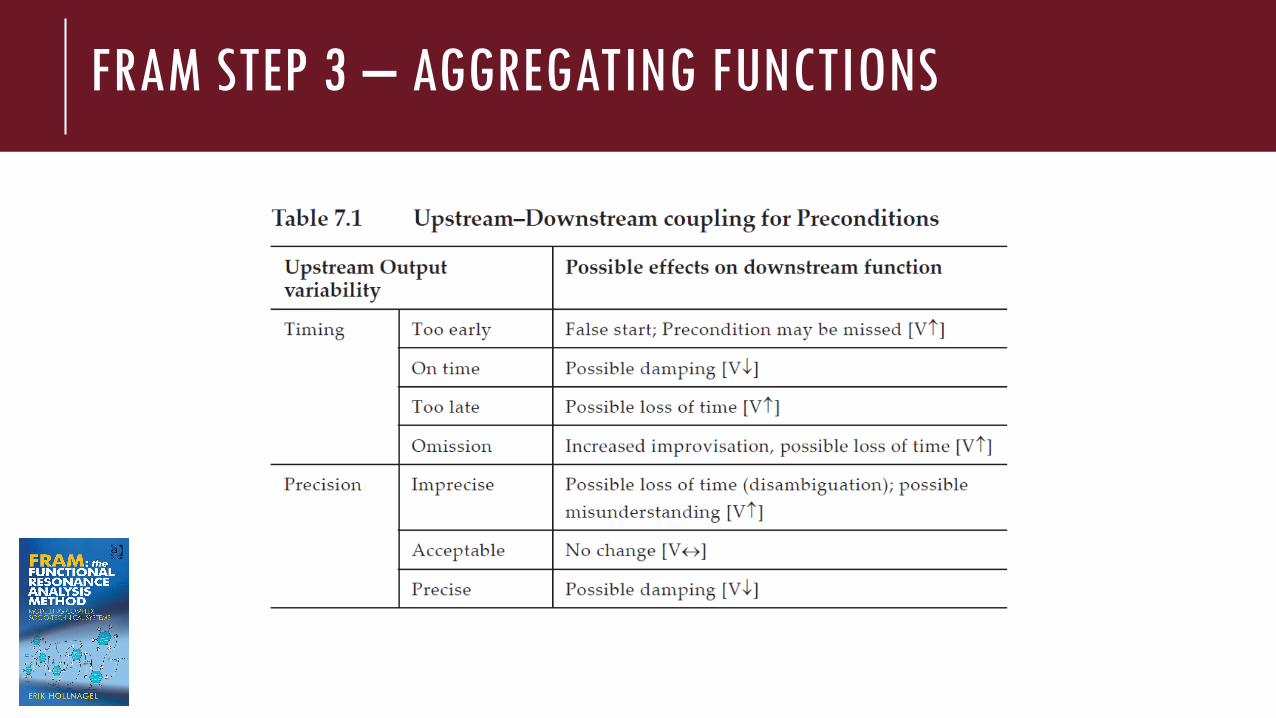
FRAM STEP 3 – AGGREGATING FUNCTIONS

𝑪𝑽𝒊𝒋 = 𝑶𝑽𝒋 ∙ 𝒂𝒊𝒋𝑻 ∙ 𝒂𝒊𝒋

𝑷

𝑎𝑖𝑗𝑇 represents the amplifying factor for the upstream output 𝑗 and the downstream function 𝑖, in terms of timing

𝑎𝑖𝑗𝑃 represents the amplifying factor for the upstream output 𝑗 and the downstream function 𝑖, in terms of precision

𝑎𝑖𝑗𝑇 (or 𝑎𝑖𝑗

𝑃 )

> 1 in case the upstream output has an amplyfing effect on the downstream function= 1 in case the upstream output has no effect on the downstream function< 1 in case the upstream output has a damping effect on the downstream function

Note that 𝑎𝑖𝑗𝑇 (or 𝑎𝑖𝑗

𝑃 ) may assume the following values:

We add damping/amplification coefficients to realte the output variability to the functions’ aspects

FRAM STEP 3 – AGGREGATING FUNCTIONS

FRAM STEP 3 – DIFFERENT INSTANTIATIONS

𝑺𝑷𝑪𝟏 𝑺𝑷𝑪𝟐 … 𝑺𝑷𝑪𝒎

Function 1 𝑏11 𝑏1

2 𝑏1𝑚

Function 2 𝑏21 𝑏2

2 𝑏2𝑚

…

Function n 𝑏𝑛1 𝑏𝑛

2 𝑏𝑛𝑚

𝑏𝑗𝑘

= 1 in case the 𝑆𝑃𝐶𝑘 has a high impact on the j function

< 1 in case the 𝑆𝑃𝐶𝑘 has a moderate impact on the j function

= 0 in case the 𝑆𝑃𝐶𝑘 has no impact on the j function

𝑏𝑗𝑘 identifies the effect of the

𝑆𝑃𝐶𝑘 on the 𝑗 function.

To define a particular instantiation of the model, it is necessary to define a specific number 𝑚of variables, capable of identifying the scenarios to analyze, i.e. Scenario Performance

Conditions 𝑆𝑃𝐶𝑘, where 𝑘 = 1,… ,𝑚, and their potential effect

A particular combination of 𝑆𝑃𝐶𝑘 constitutes an operating scenario. It is possible to build the S matrix, which relates each scenario to the identified 𝑆𝑃𝐶𝑘, by the 𝑆𝑃𝐶𝑧

𝑘. 𝑆𝑃𝐶𝑧𝑘

represents the 𝑆𝑃𝐶𝑘 amplifying effect in the z scenario 𝑆𝑧, 𝑧 = 1,… , 𝑍

FRAM STEP 3 – DIFFERENT INSTANTIATIONS

𝑺𝑷𝑪𝟏 𝑺𝑷𝑪𝟐 … 𝑺𝑷𝑪𝒎

Instantiation 1 𝑆𝑃𝐶11 𝑆𝑃𝐶1

2 𝑆𝑃𝐶1𝑚

Instantiation 2 𝑆𝑃𝐶21 𝑆𝑃𝐶2

2 𝑆𝑃𝐶2𝑚

…

Instantiation Z 𝑆𝑃𝐶𝑍1 𝑆𝑃𝐶𝑍

2 𝑆𝑃𝐶𝑍𝑚

𝑆𝑃𝐶𝑧𝑘 =

𝑆𝑃𝐶𝑧𝑘′ 𝐻𝑖𝑔ℎ 𝑉𝑎𝑟𝑖𝑎𝑏𝑖𝑙𝑖𝑡𝑦 𝑒𝑓𝑓𝑒𝑐𝑡 𝑜𝑓 SPCk

𝑆𝑃𝐶𝑧𝑘′′ 𝐿𝑜𝑤 𝑉𝑎𝑟𝑖𝑎𝑏𝑖𝑙𝑖𝑡𝑦 𝑒𝑓𝑓𝑒𝑐𝑡 𝑜𝑓 SPCk

𝑆𝑃𝐶𝑧𝑘′′′ 𝑁𝑜 𝑉𝑎𝑟𝑖𝑎𝑏𝑖𝑙𝑖𝑡𝑦 𝑒𝑓𝑓𝑒𝑐𝑡 𝑜𝑓 SPCk

𝑆𝑃𝐶𝑧𝑘 =

210

FRAM STEP 3 – DIFFERENT INSTANTIATIONS

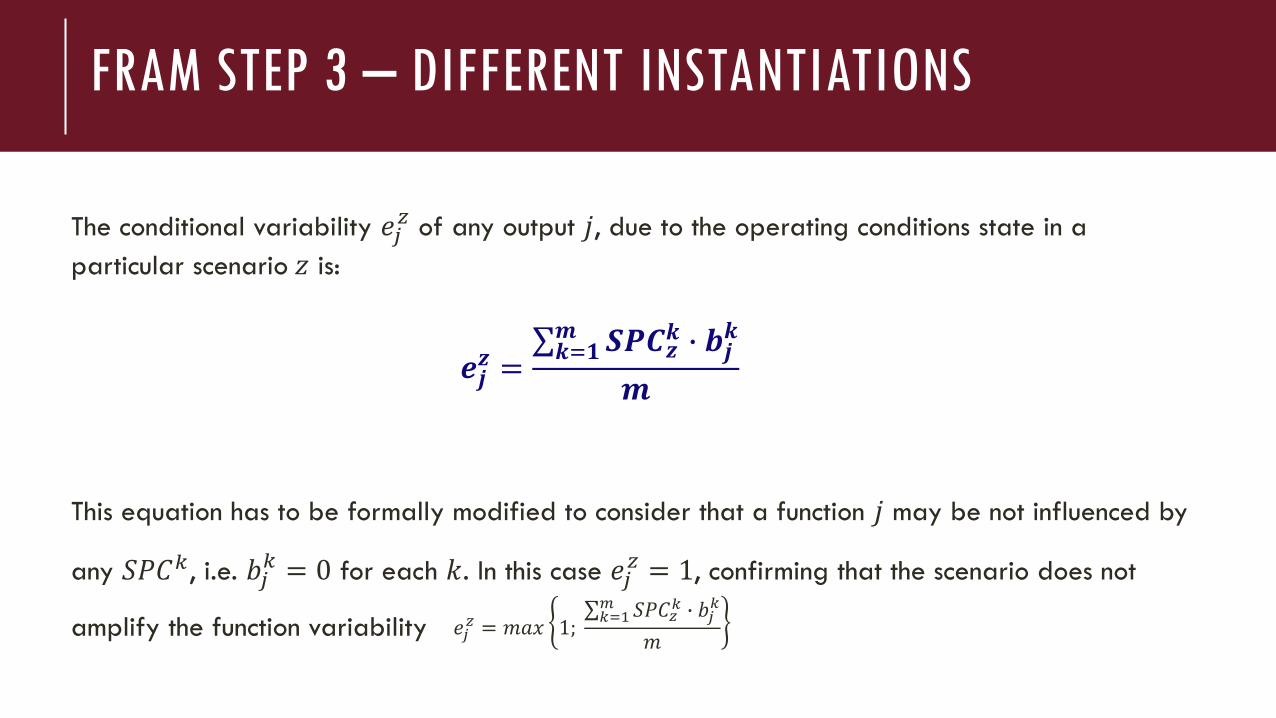
The conditional variability 𝑒𝑗𝑧 of any output 𝑗, due to the operating conditions state in a

particular scenario 𝑧 is:

𝒆𝒋𝒛 =

𝒌=𝟏𝒎 𝑺𝑷𝑪𝒛

𝒌 ∙ 𝒃𝒋𝒌

𝒎

This equation has to be formally modified to consider that a function 𝑗 may be not influenced by

any 𝑆𝑃𝐶𝑘, i.e. 𝑏𝑗𝑘 = 0 for each 𝑘. In this case 𝑒𝑗

𝑧 = 1, confirming that the scenario does not

amplify the function variability 𝑒𝑗𝑧 = 𝑚𝑎𝑥 1;

𝑘=1𝑚 𝑆𝑃𝐶𝑧

𝑘 ∙ 𝑏𝑗𝑘

𝑚

𝑽𝑷𝑵𝒊𝒋𝒛 = 𝑽𝒋

𝑻 ∙ 𝑽𝒋𝑷 ∙ 𝒂𝒊𝒋

𝑻 ∙ 𝒂𝒊𝒋𝑷 ∙ 𝒆𝒋

𝒛

FRAM STEP 3 – OVERALL INDEX

The overall index for each coupling, which address its variability according timing and precision phenotypes, in an operating scenario z can be derived as:

function

variability

upstream/

downstream

link

scenario

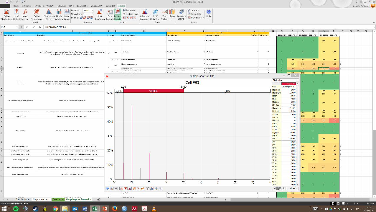
Once assigned the variability following the distributions, it is possible to define criticalcouplings and paths, based on the 𝑽𝑷𝑵𝒊𝒋

𝒛 and then mitigating actions.

A coupling is considered critical if the cumulative distribution over a threshold is minor than a confidence level.

FRAM STEP 4

The distribution in this area (for example) represents

possible combinations of variability with critical

impact on performance (if minor than the confidence

level, the coupling becomes critical)

SIMPLE SOLUTION: IS IT ALWAYS ENOUGH?

T I M E

P R E C I S I O N

S P E E D

O B J E C T

D I R E C T I O N

F O R C E

Nominal

Too late or too early

- no impact on

mission success and

safety

Too late or too early

- low impact on

mission success

Too late or too early

- impact on mission

success and safety

1 2 3 4

Nominal

Acceptable - no

impact on mission

success and safety

Imprecise - low

impact on mission

success

Imprecise - impact

on mission success

and safety

1 2 3 4

Nominal

Too slow or too fast

- no impact on

mission success and

safety

Too slow or too fast

- low impact on

mission success

Too slow or too fast

- impact on mission

success and safety

1 2 3 4

Nominal Detectable FailedNot Detectable

Failed

1 3 4

Nominal

Not nominal

direction - no

impact on mission

success and safety

Imprecise direction -

low impact on

mission success

Wrong direction -

impact on mission

success and safety

1 2 3 4

Nominal

Too much or too

little - no impact on

mission success and

safety

Too much or too

litlle - low impact on

mission success

Too much or too

little - impact on

mission success and

safety

Score

Possible Output variability with regard to object

Score

Possible Output variability with regard to time

Score

Possible Output variability with regard to precision

Score

PH=1

Time

variability

PH=2

Precision

Variability

PH=3

Speed

Variability

PH=4

Possible Output variability with regard to speed

Object

Variability

PH=5

Direction

Variability

PH=6

Possible Output variability with regard to direction

Score

Possible Output variability with regard to force

Force

Variability

Each function variability can be described

by six phenotypes of variability

COMPLEX SOLUTION

𝑶𝑽𝒋 = 𝑽𝒋𝑻 ∙ 𝑽𝒋

𝑷 ∙ 𝑽𝒋𝑺 ∙ 𝑽𝒋

𝑶∙ 𝑽𝒋𝑫 ∙ 𝑽𝒋

𝑭

We develop the Phenotype Rule Block (PRB)

Multiplying the factors

is not statistically representative

COMPLEX SOLUTION

Similarly, for evaluating the coupling we develop the Coupling Rule Block (CRB), which allows defining

the Variability Priority Number (VPNij) of each coupling.

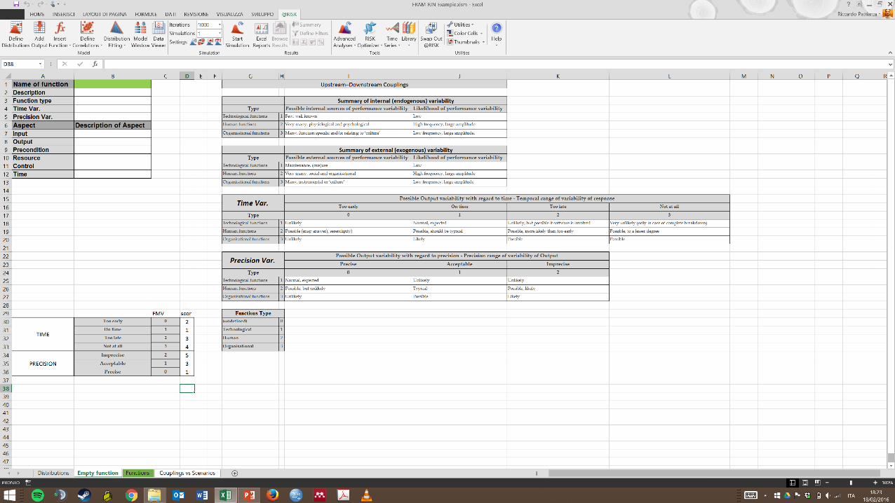
This approach required an IT support tool, and so we developed a VBA-based code

THAT’S «FUNNY», BUT HOW TO APPLY IT?

FRAM Model

Visualizer

MS ExcelPalisade @Risk

WALKTHROUGH

A brief description of how the tool works and how it could help our analysis

Just a summary…

Estimate distribution’s parameters

HOW TO DEFINE THE DISTRIBUTIONS’ PARAMETERS?

Chategorize functions into

H/T/O

Retrieve data from literature

Run Monte

Carlo

simulation

Isolate critical

paths

Develop

dedicate

report forms

for everyday

work

Analyze the

reports

FRAM model(the traditional

one)

Data from sharp-end reports

(simulation, judgments,etc.)

Define mitigating actions(improve training, change a procedure, etc.)

EXAMPLE OF APPLICATION: RUNWAY INCURSION

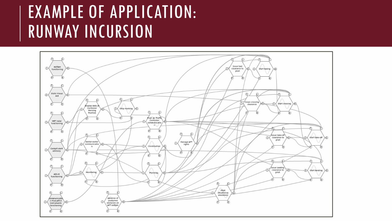
EXAMPLE OF APPLICATION: RUNWAY INCURSION

Downstream function Upstream function Scenarios

Name of

functionAspect

Name of

function

Description

of Aspect

Scenario

1

Scenario

2

Scenario

3

Scenario

4

Scenario

5

Scenario

6

Absence of

undesired

obstacles on APT

surface

ControlNOTAM

functioningNOTAM issued 0 0 0 0 0.004 0.004

Sector-sector

communication

InputADS-B

functioningADS-B data 0 0 0 0 0.004 0.004

Resource CoordinationCoordinated

personnel0 0.001 0.001 0.001 0.001 0.001

Pilot/ATCO

communication

Input

Communication

Pilot/ATCO

instruments

functioning

Pilot/ATCO

communication

link active

0 0.001 0.001 0.158 0.158 0.158

Start crossing InputPilot/ATCO

communication

Clarified

instructions0 0.275 0.275 0.275 0.275 0.770

EXAMPLE OF APPLICATION: RUNWAY INCURSION

EXAMPLE OF APPLICATION: APOLLO 11 POWERED DESCENT

http://history.nasa.gov/afj/

Presented at the 8th IAASS Conference on Advancement of Space Safety (18-20 May 2016, Melbourne, FL)

EXAMPLE OF APPLICATION: APOLLO 11 POWERED DESCENT

EXAMPLE OF APPLICATION: APOLLO 11 POWERED DESCENT

Railway safety

Ground Handling safety

Healthcare (perioperative care)

Industrial plants

…

OUR CURRENT RESEARCH THEMES…

Now have a look to our tool and our VBA code

A WALKTHROUGH THE CODE

FRAM Model

Visualizer

MS ExcelPalisade @Risk

One of the most serious accidents ever happened:

Deaths: >1’000’000

Destroyed more than 18 highly technolgical planes

What is this?

Have a look to this video!

AND NOW…A «SERIOUS» REFLECTION

« Great shot kid, that was one in a million »

Han Solo, Star Wars Ep. IV

Death star seems an ultrasafe system, so my questions are…(may be you need to look again the films)

If you were an imperial soldier, how would you prevent the death star’s destruction?

If a rebel, how to make that distruction just not a lucky case (due to Luke’s jedi skills)?

and moreover..

Do you think is it useful to «filter» the traditional functions?

Which way of filtering them is the most useful one?

Is a multi-layer representaion really useful?

Do you think is it useful an Excel-based representation?

Would you like to use this Excel tool? Do you think is there required any modifications?

AND SEVERAL FUTURE SERIOUS CHALLENGES

THANK YOU ALL

MAY THE…FRAM BE WiTH You