monte carlo simulation of solid rocket exhaust plumes...
TRANSCRIPT
Monte Carlo Simulation of Solid Rocket Exhaust Plumes at High Altitude
by
Jonathan Matthew Burt
A dissertation submitted in partial fulfillment of the requirements for the degree of
Doctor of Philosophy (Aerospace Engineering)
in The University of Michigan 2006
Doctoral Committee:
Professor Iain D. Boyd, Co-Chair Professor Wei Shyy, Co-Chair Professor Philip L. Roe Research Professor Michael R. Combi

© Jonathan Matthew Burt
All rights reserved
2006

To my parents, and to Alissa.
ii
Acknowledgements
I’d first like to thank my advisor, Prof. Iain Boyd, for continual guidance and
encouragement over the last four years. Much of my work, knowledge and interest in
rarefied gas dynamics is a result of your teaching and oversight, and I am grateful for the
opportunity you have given me to pursue this as a career path. I’d also like to
acknowledge my committee members, Profs. Shyy, Roe and Combi, and all of the other
faculty members who have provided suggestions, answered questions, and in many other
ways made my graduate school experience more productive and enjoyable.
A number of other people have provided important input for the research presented in
this thesis. While there are far too many to name here, I’d like to acknowledge a few
people who have been particularly helpful, and without whom I would not have been able
to perform much of my dissertation research. First, I’d like to thank Tom Smith, Dean
Wadsworth and Jay Levine at the Air Force Research Laboratory for overseeing my
research and for providing the generous financial support that enabled me to perform this
work. Ingrid Wysong, Sergey Gimelshein and Matt Braunstein have also been
enormously helpful over the past several years, through their many suggestions and
comments, and through the discussions and e-mail exchanges we have had on the
progress and direction of my research.
iii

My experience at the University of Michigan would have been far less enjoyable had
it not been for the many students I have met and friends I have gained while here. Again I
cannot name everyone, but in particular I’d like to thank Anish, Yoshi, Matt, Anton,
Michael M., John Y., Jose, Kooj, Jerry, Tom, Allen, Andy, Andrew, Javier P., Javier D.,
Quanhua, Leo, Dave and Chunpei. You have helped me to grow and mature as a student,
a researcher and an individual.
I’d also like to thank my family, and particularly my parents, for your unconditional
support and encouragement, and for providing me with the self confidence and
motivation that has allowed me to become the person that I am today. Lastly, I’d like to
thank Alissa, for your comfort and support during my time spent writing this thesis, and
for the happiness you have brought to me.
iv
Table of Contents
Dedication ii
Acknowledgements iii
List of Figures ix
List of Tables xiii
List of Appendices xiv
Chapter
I. Introduction and Background 1
1.1 Applications of solid rocket plume analysis 1 1.2 The physics of high altitude SRM exhaust flows 4 1.2.1 Particle formation inside the motor 5 1.2.2 Particle phase change 6 1.2.3 Gas properties in the plume 9 1.2.4 The farfield plume region 10 1.3 A short history of high altitude SRM exhaust flow modeling efforts 11 1.3.1 Nozzle flow simulations 13 1.3.2 Continuum approaches for simulating high altitude plume flows 17 1.3.3 The direct simulation Monte Carlo method 19 1.4 Outline of the thesis 22
II. The Simulation of Small Particles in a Rarefied Gas 27
2.1 The two phase DSMC approach 27 2.2 Application to a free expansion flow 31 2.2.1 Evaluation of the two phase simulation method 32 2.2.2 Additional results 44 2.3 Simulation of nonspherical particles 52 2.3.1 Collision angle distribution function 54
v

2.3.2 Average collision cross section 55 2.3.3 Effective particle size and density 56 2.4 Extension to rotating particles 57 2.4.1 The potential importance of particle rotation 57 2.4.2 The Green’s function approach 59 2.4.3 Force on a rotating particle 61 2.4.4 Moment due to particle rotation 64 2.4.5 Heat transfer rate 65 2.4.6 DSMC Implementation 69
III. Numerical Procedures for Two-Way Coupled Flows 70
3.1 Derivation of a model for two-way coupling 70 3.1.1 Specular reflection 71 3.1.2 Diffuse reflection 72 3.1.3 Two-way coupling in DSMC 75 3.2 Demonstration of momentum and energy conservation 79 3.2.1 Simulation parameters 80 3.2.2 Results and discussion 81 3.3 Two-way coupling procedures for rotating particles 87
IV. Additional Models for SRM Plume Simulation 91
4.1 Overview 91 4.2 Interphase coupling parameters 93 4.2.1 Gas-to-particle momentum coupling 94 4.2.2 Particle-to-gas momentum coupling 96 4.2.3 Gas-to-particle energy coupling 96 4.2.4 Particle-to-gas energy coupling 98 4.2.5 Implementation in DSMC 99 4.3 Particle phase change 100 4.4 Application to a representative plume flow 104 4.4.1 Simulation parameters 104 4.4.2 Variation in calculated flow properties with cutoff values 106 4.4.3 Relation between cutoff values and simulation efficiency 112 4.4.4 Additional results 114
V. An Alternate Approach for Gas Simulation in Near-Equilibrium Regions 116
5.1 Overview and motivation 116 5.1.1 Problems inherent in the DSMC simulation of SRM plume flows 117 5.1.2 The NS-DSMC hybrid approach 119 5.1.3 An all-particle hybrid scheme 120 5.2 Numerical procedure 123 5.2.1 Reassignment of particle velocities 123 5.2.2 Rotational energy resampling 126
vi
5.2.3 Momentum and energy conservation 129 5.2.4 A correction factor for the rotational relaxation rate 131 5.3 Homogeneous rotational relaxation 133 5.4 Nozzle flow simulation 135 5.4.1 Simulation setup and boundary conditions 136 5.4.2 Comparison of flowfield property contours 138 5.4.3 Centerline property variation 140 5.4.4 Comparison of results along a radial plane 143 5.4.5 Evaluation of continuum breakdown 147 5.4.6 Considerations of computational expense 149
VI. A Monte Carlo Model for Particle Radiation 153
6.1 Introduction 153 6.2 Radiation modeling procedures 156 6.2.1 Determination of initial power for an energy bundle 157 6.2.2 Procedures for absorption and scattering 159 6.2.3 Contribution to the particle energy balance 162 6.2.4 Nozzle searchlight emission 164 6.2.5 Plume radiance calculations 166 6.3 Extension to soot particles 169
VII. Simulation of a Representative Plume Flow 173
7.1 Background and simulation setup 173 7.1.1 Application to the BSUV-2 plume flow 174 7.1.2 Gas phase calculations 175 7.1.3 Boundary conditions 177 7.1.4 Plume radiation properties 178 7.1.5 Additional simulation parameters 181 7.1.6 Test for grid convergence 183 7.2 Simulation results 184 7.2.1 Gas bulk velocity 185 7.2.2 Gas and particle mass density 186 7.2.3 Particle temperatures 190 7.2.4 Particle phase change 193 7.2.5 Convective and radiative heat transfer rates 195 7.2.6 Radiative energy flux 198 7.2.7 Plume spectral radiance 201 7.3 Parametric study for gas/particle interaction 206 7.3.1 Additional simulations for comparison 207 7.3.2 Gas translational temperature 209 7.3.3 Temperature of small particles 211 7.3.4 Temperature of large particles 213 7.3.5 Radiative energy flux 215 7.3.6 UV spectral radiance 217
vii
7.4 Parametric study for particle radiation 218 7.4.1 Additional simulations 219 7.4.2 Effect of particle radiation on the gas 220 7.4.3 Particle temperatures 221 7.4.4 Radiative energy flux 223 7.4.5 UV spectral radiance 225 7.5 Potential influence of soot on plume radiation 227 7.5.1 Soot concentration and input parameters 228 7.5.2 Soot density and temperature 229 7.5.3 Radiative energy flux 232 7.5.4 UV spectral radiance 234
VIII. Summary and Future Work 236
8.1 Summary 236 8.2 Modeling difficulties and proposed future work 240 8.2.1 Unified nozzle/plume flow simulations 240 8.2.2 Monte Carlo methods for near-equilibrium flows 241 8.2.3 Gas radiation modeling 243 8.2.4 Radiation modeling for Al2O3 particles 244 8.2.5 The need for future experiments 245
Appendices 246
Bibliography 259
viii

List of Figures
Figure 2.1 Grid geometry and boundary conditions. 33
2.2 Contours of gas Mach number for a source pressure of 34.5 mmHg. 38
2.3 Particle number flux profiles along outflow boundary. 38
2.4 Values of 1/A2 as a function of source pressure, based on the numerical results.
41
2.5 Source pressure vs. experimental values of δ. 41
2.6 Variation with source pressure of terminal particle velocity along the central axis.
42
2.7 Comparison of relative particle Mach numbers along the central axis for simulations at three different source pressures.
45
2.8 Particle speed along the central axis. 45
2.9 Drag force on particles along the central axis. 46
2.10 Particle Knudsen number along the central axis. 46
2.11 Magnitude of the average particle heat transfer rate along the axis. 49
2.12 Variation along the axis in average particle temperatures. 50
2.13 Fractional change in average particle speed associated with an increase in particle temperature.
51
2.14 Angles used to determine the mean tangential velocity <ut>. 62
3.1 Coordinate systems and angles used in the evaluation of f(δ) for diffuse reflection.
72
3.2 Comparison of distribution functions for the deflection angle δ. 75
ix

3.3 Grid dimensions and boundary types. 80
3.4 Longitudinal variation in average gas and particle speeds. 82
3.5 Gas and particle number densities. 83
3.6 Variation in gas and particle temperatures. 83
3.7 Variation in longitudinal momentum transfer rates with downstream distance.
84
3.8 Energy transfer rates for gas and particles. 84
4.1 Maximum downstream distance for interphase coupling. 107
4.2 Axial velocity component for 0.3 µm diameter particles as a function of cutoff value C1 for gas-to-particle coupling.
107
4.3 Axial velocity component for 1 µm particles as a function of cutoff value. 108
4.4 Axial velocity component for 6 µm particles as a function of cutoff value. 108
4.5 Temperature of 0.3 µm particles as a function of cutoff value. 109
4.6 Temperature of 1 µm particles as a function of cutoff value. 109
4.7 Temperature of 6 µm particles as a function of cutoff value. 110
4.8 Variation in liquid mass fraction for 1 µm particles. 110
4.9 Total cpu time per time step at steady state, normalized by CPU time for the zero cutoff values case.
113
4.10 Contours of mass-averaged particle temperature (top) and gas translational temperature.
115
4.11 Sauter mean particle diameter (top) and liquid mass fraction of particles. 115
5.1 Time variation in temperatures for rotational relaxation. 134
5.2 Grid geometry for ES-BGK and DSMC simulations. 137
5.3 Mach number contours for ES-BGK (top) and DSMC (bottom). 139
5.4 Density contours for ES-BGK (top) and DSMC (bottom). 140
5.5 Density variation along the nozzle centerline. 141
5.6 Variation of rotational and translational temperature along the centerline. 142
5.7 Density variation along a radial plane at x/Rt=18.7. 143
5.8 Temperature variation along a radial plane at x/Rt=18.7. 144
5.9 Axial velocity profiles at x/Rt=18.7. 146
x

5.10 Continuum breakdown parameters along the nozzle centerline. 148
7.1 Grid geometry for simulations of the BSUV-2 flow. 175
7.2 Domains for DSMC and ES-BGK simulation methods. 177
7.3 Measured IR absorption index values for Al2O3. 179
7.4 UV absorption index values for Al2O3. 180
7.5 Sensor viewing regions for plume radiance calculations. 182
7.6 Gas translational temperature along the extraction line. 184
7.7 Location of the extraction line. 184
7.8 Gas streamlines and contours of bulk velocity magnitude. 186
7.9 Contours of mass density for particle and gas. 187
7.10 Contours of average particle diameter and Sauter mean diameter. 188
7.11 Average temperature contours for 0.4 and 4 µm diameter particles. 191
7.12 Close-up view of particle temperature contours. 192
7.13 Contours of liquid mass fraction for 4 and 6 µm diameter particles. 194
7.14 Magnitude of average convective and radiative heat transfer rates per particle along the centerline.
196
7.15 Contours of the direction-averaged spectral energy flux at wavelengths of 2.2 µm and 0.24 µm.
198
7.16 Spectral radiance at onboard and remote sensors. 201
7.17 UV spectral radiance measured at the onboard sensor. 203
7.18 Gas translational temperature along the extraction line. 210
7.19 Temperature variation along the extraction line for 0.4 µm particles. 212
7.20 Temperature variation along the extraction line for 4 µm particles. 214
7.21 Net direction-averaged radiative energy flux along the extraction line. 216
7.22 UV spectral radiance at the onboard sensor. 218
7.23 Temperature of 0.4 µm particles along the extraction line. 222
7.24 Temperature of 4 µm particles along the extraction line. 222
7.25 Variation along the extraction line in the net direction-averaged radiative energy flux.
224
7.26 Dependence of UV spectral radiance on radiation model parameters. 226
xi

7.27 Contours of soot mass and average temperature. 230
7.28 Contours of soot temperature for simulations with and without Al2O3 particles.
231
7.29 Effect of soot on the net radiative energy flux along the extraction line. 233
7.30 Effect of soot on UV radiance at the onboard sensor. 235
xii

List of Tables
Table 1.1 Approaches for SRM nozzle simulation. 12
1.2 Approaches for high altitude SRM plume simulation. 13
4.1 Particle properties at the nozzle exit. 105
xiii

List of Appendices
Appendix A. Nomenclature 247
B. Derivation of a Formula for the Deflection Angle 257
xiv

Chapter I
Introduction and Background
1.1 Applications of solid rocket plume analysis
Propulsion of aircraft and spacecraft through the combustion of solid fuels has both
an extensive history and a wide range of applications. For reasons of production cost, low
maintenance, simplicity, scalability and safety, solid propellant motors have for the past
several decades been a popular alternative to liquid-based chemical rocket propulsion
systems. Solid rocket motors (SRMs) have found wide use as a means of satellite orbit
insertion and orbit transfer, as well as in ballistic missile defense systems and similar
applications where the lack of throttle control or reignition capabilities are outweighed by
cost savings or safety advantages over liquid propellant rocket engines.
While most liquid propellant engines consist of a large number of components,
including fuel and oxidizer pumps, temperature control systems, storage tanks and a
separate combustion chamber, a typical SRM has a relatively simple structure consisting
of a large enclosure where the propellant grain is both stored and combusted, and a
convergent-divergent (De Laval) nozzle where combustion products are accelerated to
provide thrust. The simple construction and lack of moving parts allow an SRM to be
constructed for considerably less expense than a liquid rocket engine with the same thrust
1
and propellant mass. At the same time, the solid propellant tends to require far less long
term maintenance and generally presents fewer safety hazards than liquid fuels, making
SRM systems preferred for applications involving storage on ships or submarines. SRM
boosters are commonly used to augment the thrust from primary propulsion systems on
satellite launch vehicles, and reusable solid rocket boosters on the space shuttle provide
much of the thrust required for orbit insertion.
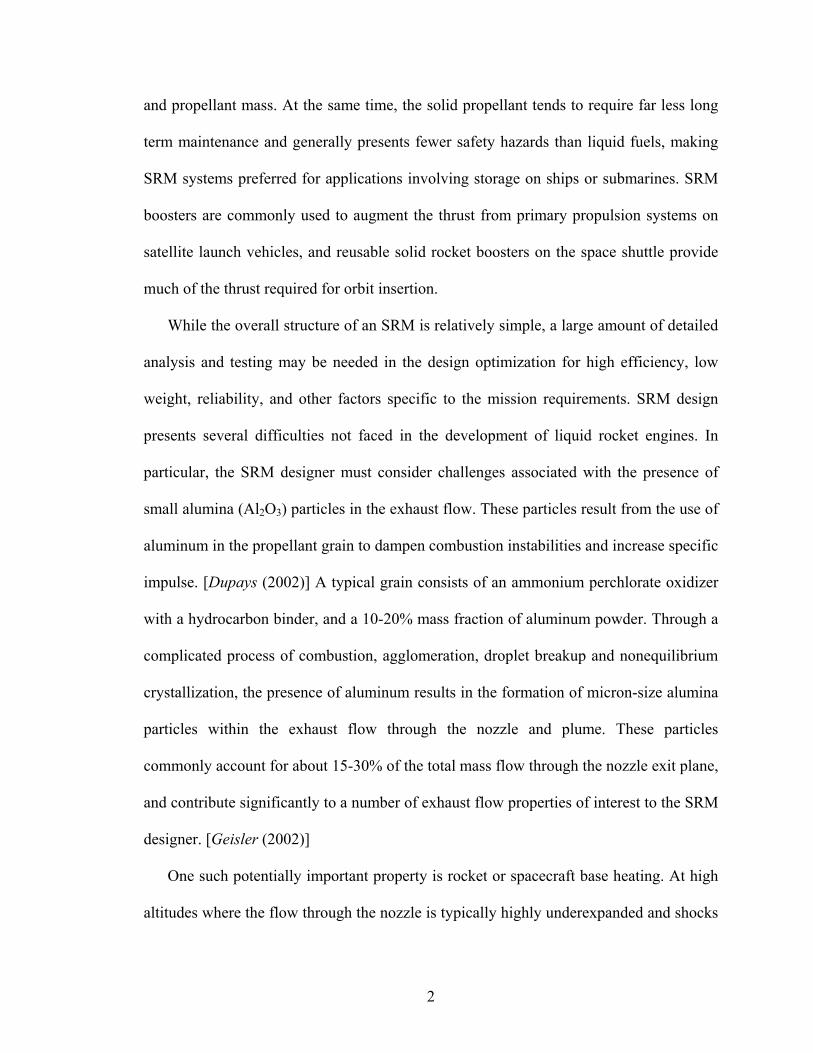
While the overall structure of an SRM is relatively simple, a large amount of detailed
analysis and testing may be needed in the design optimization for high efficiency, low
weight, reliability, and other factors specific to the mission requirements. SRM design
presents several difficulties not faced in the development of liquid rocket engines. In
particular, the SRM designer must consider challenges associated with the presence of
small alumina (Al2O3) particles in the exhaust flow. These particles result from the use of
aluminum in the propellant grain to dampen combustion instabilities and increase specific
impulse. [Dupays (2002)] A typical grain consists of an ammonium perchlorate oxidizer
with a hydrocarbon binder, and a 10-20% mass fraction of aluminum powder. Through a
complicated process of combustion, agglomeration, droplet breakup and nonequilibrium
crystallization, the presence of aluminum results in the formation of micron-size alumina
particles within the exhaust flow through the nozzle and plume. These particles
commonly account for about 15-30% of the total mass flow through the nozzle exit plane,
and contribute significantly to a number of exhaust flow properties of interest to the SRM
designer. [Geisler (2002)]
One such potentially important property is rocket or spacecraft base heating. At high
altitudes where the flow through the nozzle is typically highly underexpanded and shocks
2

due to plume-atmosphere interaction are suppressed, the alumina particles tend to
develop large temperature lags relative to the surrounding gas. Particle emission may
dominate the radiative energy balance throughout the plume, and contribute greatly to
radiative heating of rocket or spacecraft components within the plume line of sight. The
surface temperatures of these components may increase by several hundred degrees due
to radiative heat transfer from the particles, so an understanding and accurate estimation
of this effect may be crucial in designing for acceptable thermal loading.
Another unwanted characteristic of alumina particles in the plume is the potential for
impingement and contamination on the rocket or spacecraft surface. One common
application of SRMs is as secondary thrusters for stage separation, orbit stabilization or
small trajectory corrections. As particles are forced outward from the nozzle centerline by
the rapidly expanding gas in a high altitude side thruster plume, there is some possibility
that particles ejected from the thruster will collide with downstream spacecraft surfaces.
This presents problems of systems operation and reliability, and must be addressed as
part of the design process.
The presence of alumina particles also creates challenges in SRM design for low
observable signatures. These particles tend to dominate plume radiative emission in much
of the IR through near-UV range (wavelengths of 0.2 to 5 µm) and may dramatically alter
the optical thickness and scattering properties of the plume as well. [Simmons (2000)] In
the development of SRM propulsion and control systems for ballistic missile
applications, accurate determination of particle radiation characteristics may therefore be
required.
3

Radiation analysis for solid rocket plumes plays another important role in the missile
defense community. Ballistic missile defense systems require a database of emission
characteristics for existing SRM designs, so that observed threats may be quickly and
accurately identified. In addition, the kill vehicle must be able to distinguish the hard
body (i.e. the rocket or reentry vehicle) from the plume, and needs to quickly identify the
target location based on IR emission characteristics.
Ideally, the required performance, contamination and radiation analysis could be
carried out through experiments involving full-scale SRM exhaust flows in low density
test chambers. Due however to the extensive time, cost, and general impracticality of this
approach, numerical simulations are a far more popular means of determining plume
properties of interest, and historically much of the effort involved in SRM plume analysis
has been devoted to the development and application of detailed numerical models.
1.2 The physics of high altitude SRM exhaust flows
While the computational analysis of high altitude solid rocket plume flows presents
several major advantages over experimental measurement, significant disadvantages do
exist in the numerical approach. A number of complex or poorly understood physical
phenomena within the combustion chamber, nozzle and plume can make accurate
simulation extremely difficult or expensive. Several potentially important physical
processes have generally been overlooked in the interest of reducing computational
expense or code complexity, and the coupling between some flowfield characteristics has
been neglected in even the most ambitious numerical studies. A number of processes
involving the alumina particles are particularly challenging to include in simulations, but
4

may need to be modeled for accurate determination of various flowfield and radiation
properties. To provide a general sense of the physical phenomena related to alumina
particle formation, size distribution, phase composition, and interaction with the
surrounding gas, a brief outline of relevant processes in SRM exhaust flows is presented
here.
1.2.1 Particle formation inside the motor
During the burning process in an SRM, aluminum particles embedded within the
propellant grain are continually exposed to the advancing surface on which most of the
combustion takes place. These exposed particles tend to rapidly melt and coalesce into
larger agglomerates, with a diameter typically on the order of 100 µm, which
immediately begin a process of surface oxidation. Some of the aluminum content on the
agglomerate surface may vaporize and react with oxygen in the surrounding gas to form a
detached flame front, while heterogeneous combustion on the particle surface creates a
liquid Al2O3 shell.
As the particle is accelerated into the intensely turbulent stream of hot exhaust gases
flowing toward the nozzle entrance, surface pressure and shear stresses tend to break off
portions of the material into smaller droplets, exposing additional unburned aluminum
and further promoting the oxidation process. A large number of micron-size liquid
droplets, termed “smoke” particles, may be sheared off the agglomerate surface during
this stage. At the nozzle entrance, the particle phase is typically made up of a bimodal
distribution of agglomerate and smoke particles, both in liquid form. [Simmons (2000),
Geisler (2002)]
5

Within the subsonic convergent nozzle region, the particle size distribution is further
modified due to breakup and agglomeration processes. As the gas rapidly expands and
accelerates in a transition from thermal to bulk kinetic energy, the agglomerate particles
develop large velocity lags relative to the surrounding gas. This increases the surface
forces on a particle, and further promotes breakup.
Due to the size dependence in the ratio of surface forces to particle mass, the velocity
lag on a particle is a strong function of its size. Within the convergent nozzle region, the
smallest particles tend to move along gas streamlines at roughly the local gas bulk
velocity. Larger particles are more gradually accelerated, and may move along
trajectories which diverge significantly from the gas streamlines. The difference in speed
and direction between particles of different sizes tends to promote collisions between
these particles. Some fraction of the collisions result in agglomeration, and the newly
created agglomerate particles then rotate according to the dynamics of off-center
coalescing collisions. This rotation in turn may trigger an additional breakup mode,
where the agglomerate breaks into smaller droplets because centrifugal forces outweigh
the restoring influence of surface tension. Ultimately, the combination of breakup and
agglomeration processes tends to produce a polydisperse particle size distribution within
the nozzle, with particles ranging in diameter from about 0.1 to 10 µm.
1.2.2 Particle phase change
As the gas and particles are accelerated through the nozzle throat, the gas temperature
quickly drops to well below the melting temperature of the particle material (about 2325
K) and particle phase change processes may begin. As with velocity lags, temperature
6

lags depend strongly on particle size due to the size dependence in the ratio of surface
heat transfer to heat capacity. While larger particles tend to retain a relatively constant
temperature (to within a few hundred K) during their course through the nozzle, smaller
sub-micron scale particles experience rapid temperature changes as a result of convective
heat transfer with the cooler surrounding gas. As a result, the smallest particles are the
first to experience phase change within the nozzle.
While the mechanics of alumina particle crystallization are extremely complicated
and not fully understood, the general processes may be summarized as follows: First,
when a liquid droplet has supercooled to some temperature well below its melting
temperature, homogeneous nucleation occurs at locations at or near the surface. (Due to
convective cooling, the surface temperature is slightly lower than the temperature at
points closer to the particle center.) Heterogeneous crystallization fronts then quickly
progress from these nucleation points to cover the surface of the particle, after which a
single unified crystallization front moves inward from the fully solidified surface. Heat
released during the phase change process tends to increase the particle temperature,
which in turn reduces the speed of the crystallization front and slows the overall rate of
phase change.
The polycrystalline lattice structure behind the front may be that of several different
metastable solid phases, collectively termed the γ phase. A further process of phase
transition immediately begins in the region behind the front, where γ phase structures are
converted to a stable α phase and some additional heat is released. [Rodionov et al.
(1998)] As this secondary phase change process is suppressed when particles are cooled
at a sufficiently fast rate, the smallest particles – those experiencing the most rapid
7

cooling – may retain a large γ phase mass fraction throughout the divergent nozzle region
and plume.
For larger particles, the crystallization process may begin well downstream of the
nozzle exit, and will continue at a significantly slower rate. This slower rate results from
the fact that convective heat transfer is reduced as the gas density decreases with
downstream distance, so the heat released during the phase change process is opposed by
a smaller heat transfer to the gas than occurs further upstream. Thus, during
crystallization the temperature of these larger particles increases to just below the melting
temperature. At this increased temperature the velocity of the crystallization front
approaches zero, and the heat release associated with phase change balances the heat lost
to convective and radiative cooling. As a result, the particle temperature may for some
time remain nearly constant. [Plastinin et al. (1998)] Another phenomenon observed in
the larger particles (greater than 2 µm in diameter) is the creation of gas bubbles thought
to contain water vapor which is exposed during the crystallization process. Scanning
electron microscope (SEM) images of alumina particles collected from an SRM exhaust
flow have been found to include hollow shells, and the measured material density for
these particles was well below that expected for solid alumina. [Gosse et al. (2003)]
One important characteristic of SRM exhaust flows is the strong dependence of the
particle size distribution on nozzle size. For a given set of chamber and atmospheric
conditions, a larger nozzle results in a more gradual acceleration of the gas. With a
greater residence time in the nozzle, large agglomerate particles may develop
significantly lower velocity lags, which inhibits breakup due to surface forces and skews
the particle size distribution at the nozzle exit in favor of larger particles. Agglomeration
8

processes within the nozzle are also affected, as particles are more likely to experience
coalescing collisions when the nozzle residence time increases. As with velocity lags,
particle temperature lags are also lower in a larger nozzle. This tends to delay the onset of
crystallization, and results in a greater mass fraction of the stable α phase further
downstream in the plume.
1.2.3 Gas properties in the plume
Due to the large mass fraction of alumina particles through much of the flowfield,
bulk properties of the exhaust gas may be significantly influenced by the presence of
these particles. Velocity lags, particularly among the larger particles, can result in two
phase flow losses, where momentum transfer between the particles and gas pushes the
sonic line at the throat somewhat further downstream and reduces the gas velocity
through much of the nozzle and plume. At the same time, interphase energy transfer may
account for an increase in gas temperatures. Heat addition to the particles through
heterogeneous combustion and crystallization results in an increase in temperature lags
between particles and the surrounding gas, while energy exchange during interphase
collisions can reduce temperature lags through an increase in gas temperatures. The effect
of the particles on the gas depends on the local particle mass fraction, which in turn is a
strong function of both location in the flowfield and aluminum content in the propellant
grain.
A typical SRM exhaust flow at high altitudes (above 100 km) is highly
underexpanded, so that the gas experiences a rapid pressure drop just downstream of the
nozzle exit. While a diffuse shock may form within the plume-atmosphere interaction
9

region far from the plume centerline, the repeating pattern of barrel shocks, shock
reflections and Mach discs found in lower altitude exhaust flows is typically absent.
[Simmons (2000)] Streamlines may curve by over 90° around the nozzle lip, so that a
backflow region forms upstream of the nozzle exit plane. In the rapid expansion
occurring within this region, the gas velocity distribution begins to diverge significantly
from the Maxwellian distribution expected at equilibrium, and thermal energy is
increasingly distributed nonuniformly among the various translational and internal
degrees of freedom. Along streamlines far from the central axis in a single-nozzle
axisymmetric exhaust flow, the gas may experience considerable thermal nonequilibrium
within a short distance of the nozzle exit. Rotational freezing can occur as a result of the
low collision frequency in this region, and flow characteristics may approach the free
molecular limit where quantities such as the scalar pressure lose their physical
significance. Similar features may be found further downstream near the plume
centerline.
1.2.4 The farfield plume region
In the rapid expansion process around the nozzle exit, both velocity and temperature
lags for the alumina particles may jump significantly, and the rate of change in particle
temperatures may fall due to the reduction in heat transfer rates associated with a drop-off
in gas density beyond the nozzle exit. As within the nozzle, velocity and temperature lags
are strong functions of particle size, so that smaller particles will be more rapidly
accelerated in both radial and axial directions following the local gas bulk velocity. As a
result, the smallest particles will experience the largest curvature in trajectories within the
10

nearfield plume region around the nozzle lip, and far downstream in the plume these
particles will have a greater maximum divergence angle than particles of larger size.
As the gas density continues to decrease with downstream distance, heat and
momentum transfer between particles and the surrounding gas becomes negligible.
Particles far downstream of the nozzle tend to move along straight trajectories at constant
velocity, and the particle energy balance within these farfield plume regions is dominated
by radiative heat transfer. Depending on the motor size and grain composition, these
regions will likely have some intermediate optical thickness, so that long-range radiative
energy exchange may significantly influence particle temperatures.
1.3 A short history of high altitude SRM exhaust flow modeling efforts
Published numerical and analytical studies of solid rocket exhaust flows may be
divided into two broad categories: those that focus on flow properties within the motor,
and those that primarily consider properties of the plume. To accurately simulate an SRM
plume flow, some detailed knowledge of gas and particle phase characteristics within the
nozzle is generally required. Studies in the second category therefore tend to rely on
results from those in the first. A brief historical outline for both types is presented here,
with an emphasis on numerical investigations of SRM exhaust flows under the typical
conditions, as described above, encountered in space or at very high altitudes. Note that
this description is not intended as a comprehensive review, but as a general overview of
historical modeling efforts with brief summaries of illustrative work over the past several
decades.
11

To clarify the following discussion of various simulation methods for SRM exhaust
flows, brief lists of methods appropriate for nozzle and plume flow simulation are
provided in Tables (1.1) and (1.2). References for a number of nozzle simulation
approaches are shown in Table (1.1), along with a short description of some advantages
and disadvantes for each approach. Table (1.2) contains similar information for the
simulation of high altitude SRM plume flows.
Method Examples Advantages Disadvantages Quasi-1D Bailey et al.
(1961), Hunter et al. (1981)
Very inexpensive May easily add physics
models, 2-way coupling
Inaccurate particle radial distribution
No boundary layers, wall interaction
Method of characteristics
Kliegel and Nickerson (1961)
Inexpensive Accounts for 2D gas
effects
Limited to divergent nozzle region
Assumes inviscid gas 2 phase CFD: Eulerian tracking
Chang (1980)
Low memory requirements
Simple 2-way coupling
Numerical diffusion Poorly suited for range
of particle sizes 2 phase CFD: Lagrangian tracking
Hwang and Chang (1988), Najjar et al. (2003)
No unphysical particle diffusion
Allows direct particle physics models
High memory requirements
Expensive Potential for scatter
Table 1.1. Approaches for SRM nozzle simulation.
12

Method Examples Advantages Disadvantages Method of characteristics
Clark et al. (1981), Rattenni (2000)
Inexpensive May apply to large
expansion angles
Assumes inviscid gas Neglects rarefaction
effects
Navier Stokes Candler et al. (1992), Vitkin et al. (1997)
Robust, efficient May easily integrate
with nozzle flow simulation
Requires empirical correlations for gas-particle interaction
Valid only for low Kn DSMC Hueser et
al. (1984) Accurate at high Kn Unconditionally stable Allows direct
molecular-level physics models
Very expensive Large memory
requirements
Table 1.2. Approaches for high altitude SRM plume simulation.
1.3.1 Nozzle flow simulations
Much of the early numerical work on SRM exhaust flows focused on gas and particle
properties in the nozzle, with an emphasis on nozzle design, efficiency and thrust
prediction. Some of these early studies are described in a review paper of Hoglund
(1962), which discusses computational and analytical treatments of two phase nozzle
flows within a few distinct categories.
The first of these categories is the quasi-one dimensional flow, where nozzle
dimensions are used to prescribe gas properties at a number of points along the length of
the nozzle, and the flow is generally assumed isentropic and chemically frozen. Particle
drag and heat transfer correlations are employed to plot the variation of velocity and
temperature through the nozzle for a given particle size. The resulting particle velocity
and temperature lags may then be used to roughly determine overall efficiency and
performance characteristics, and particle loss terms can be brought into the governing
equations for the gas to account for two phase flow losses. In one of the most ambitious
13

of these early studies, Bailey et al. (1961) compute the quasi-one dimensional nozzle
flow solution for a reacting gas, and use a post-processing approach to determine the two
dimensional trajectories and temperatures for particles of various sizes through the
nozzle.
In a more complicated treatment, the method of characteristics (MOC) is employed to
model a supersonic inviscid gas flow through the divergent portion of the nozzle, and
representative particles are tracked through the resulting flowfield using a Lagrangian
scheme. This allows the inherently two dimensional nature of the gas flowfield solution
to influence particle properties, and provides a somewhat more realistic approximation of
the nozzle flow problem. Kliegel and Nickerson (1961) apply this technique with a
modification for two-way coupling, where bulk gas properties downstream of the nozzle
throat are affected by the presence of the particle phase.
With advances in both computer power and numerical schemes, later efforts at SRM
nozzle simulation have involved progressively greater complexity and physical modeling
capabilities. Around two decades after the first quasi-one dimensional studies appear in
the literature, Chang (1980) presents results from a series of geometrically complex two
phase flows through the transonic portion of the nozzle. A finite difference Eulerian
formulation is used to compute properties for both the gas and particles, and source terms
in the governing equations for each phase allow for potentially strong two way interphase
coupling of momentum and energy. While the gas is assumed chemically frozen and
inviscid (with the exception of viscous characteristics in gas-particle interaction) the
model does incorporate effects such as particle radiative heat loss and variable particle
velocity and temperature lags through regions of subsonic as well as supersonic flow.
14
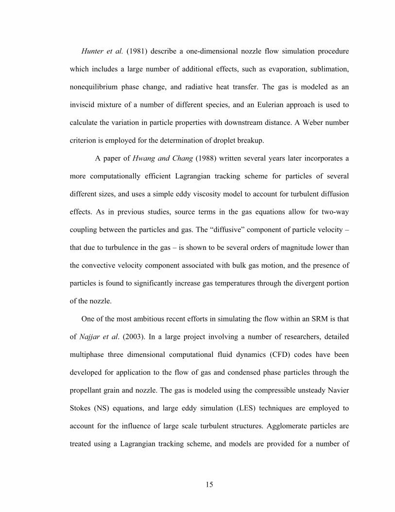
Hunter et al. (1981) describe a one-dimensional nozzle flow simulation procedure
which includes a large number of additional effects, such as evaporation, sublimation,
nonequilibrium phase change, and radiative heat transfer. The gas is modeled as an
inviscid mixture of a number of different species, and an Eulerian approach is used to
calculate the variation in particle properties with downstream distance. A Weber number
criterion is employed for the determination of droplet breakup.
A paper of Hwang and Chang (1988) written several years later incorporates a
more computationally efficient Lagrangian tracking scheme for particles of several
different sizes, and uses a simple eddy viscosity model to account for turbulent diffusion
effects. As in previous studies, source terms in the gas equations allow for two-way
coupling between the particles and gas. The “diffusive” component of particle velocity –
that due to turbulence in the gas – is shown to be several orders of magnitude lower than
the convective velocity component associated with bulk gas motion, and the presence of
particles is found to significantly increase gas temperatures through the divergent portion
of the nozzle.
One of the most ambitious recent efforts in simulating the flow within an SRM is that
of Najjar et al. (2003). In a large project involving a number of researchers, detailed
multiphase three dimensional computational fluid dynamics (CFD) codes have been
developed for application to the flow of gas and condensed phase particles through the
propellant grain and nozzle. The gas is modeled using the compressible unsteady Navier
Stokes (NS) equations, and large eddy simulation (LES) techniques are employed to
account for the influence of large scale turbulent structures. Agglomerate particles are
treated using a Lagrangian tracking scheme, and models are provided for a number of
15
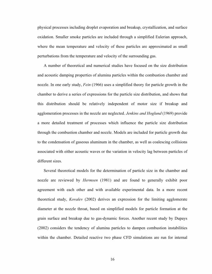
physical processes including droplet evaporation and breakup, crystallization, and surface
oxidation. Smaller smoke particles are included through a simplified Eulerian approach,
where the mean temperature and velocity of these particles are approximated as small
perturbations from the temperature and velocity of the surrounding gas.
A number of theoretical and numerical studies have focused on the size distribution
and acoustic damping properties of alumina particles within the combustion chamber and
nozzle. In one early study, Fein (1966) uses a simplified theory for particle growth in the
chamber to derive a series of expressions for the particle size distribution, and shows that
this distribution should be relatively independent of motor size if breakup and
agglomeration processes in the nozzle are neglected. Jenkins and Hoglund (1969) provide
a more detailed treatment of processes which influence the particle size distribution
through the combustion chamber and nozzle. Models are included for particle growth due
to the condensation of gaseous aluminum in the chamber, as well as coalescing collisions
associated with either acoustic waves or the variation in velocity lag between particles of
different sizes.
Several theoretical models for the determination of particle size in the chamber and
nozzle are reviewed by Hermsen (1981) and are found to generally exhibit poor
agreement with each other and with available experimental data. In a more recent
theoretical study, Kovalev (2002) derives an expression for the limiting agglomerate
diameter at the nozzle throat, based on simplified models for particle formation at the
grain surface and breakup due to gas-dynamic forces. Another recent study by Dupays
(2002) considers the tendency of alumina particles to dampen combustion instabilities
within the chamber. Detailed reactive two phase CFD simulations are run for internal
16

SRM exhaust flows, and a correlation is found between aluminum combustion and
unsteady flow properties in the gas.
1.3.2 Continuum approaches for simulating high altitude plume flows
While a number of computational studies have focused on the characteristics of low
altitude plume flows from solid propellant rockets (see, for example, Dash et al. (1985))
the two phase simulation of high altitude SRM plumes has a comparatively recent and
sparse history. In what may be one of the first such numerical studies, Clark, Fisher and
French (1981) consider the distribution of alumina particles in the plume back-flow
region for an SRM exhausting into a vacuum. An uncoupled method of characteristics
(MOC) approach is used to determine gas properties in the plume, and corrections are
made for boundary layer growth along the inner wall of the nozzle. Representative
particles are then tracked through the plume using a predictor-corrector technique. Forces
on these particles are determined through a rough empirical correlation for the particle
drag coefficient.
A similar simulation procedure has been used more recently by Rattenni (2000) to
calculate convective and radiative surface heat transfer rates from a spacecraft-mounted
SRM used for orbit insertion. A quasi-one dimensional method is employed to determine
gas properties and species concentrations within the nozzle, with an equilibrium
chemistry model in the convergent nozzle region and a model for turbulent boundary
layer growth along the nozzle wall. A MOC technique is used to model both the gas and
particles within the plume, where the particle phase consists of five discrete sizes and
some modeling capabilities are included for droplet crystallization. Particle radiative heat
17

transfer is then computed through a post-processing approach, following assumptions that
gas phase IR emission is negligible and the plume is optically thin.
In the early 1990s a series of two phase CFD calculations were performed to simulate
the SRM plume flow from a high altitude flight experiment [Erdman et al. (1992)]
involving UV radiation measurements from a set of onboard sensors. Candler et al.
(1992) present results from axisymmetric simulations at altitudes between about 105 and
120 km, where gas properties are computed using the steady state compressible NS
equations and an Eulerian approach is used for particle phase calculations. Spectral
radiance is measured through a line-of-sight procedure which assumes that the gas is
transparent and the particle phase is optically thin. There is reasonable agreement in the
shape of the UV radiance profile between the calculations and experimental data,
although particle phase enthalpies at the nozzle exit must be modified by a nonphysical
scaling factor for quantitative agreement.
As discussed by these authors, the NS equations are likely invalid under the highly
rarefied conditions expected through much of the flowfield, so a continuum-based CFD
approach can at best give only rough approximations of flowfield properties through the
plume. Slightly better agreement with experimental radiance values is found through a
similar set of two phase CFD simulations by Anfimov et al. (1993) where particle
emissive properties are determined by a complicated system of absorption index
correlations for four different mechanisms of intrinsic radiation from liquid or solid phase
alumina.
In a comprehensive numerical study on plume radiation by Vitkin et al. (1997) a
simulation is performed for a two phase axisymmetric SRM plume expanding into a
18

vacuum. An Eulerian description is used for the alumina particles, and the governing
equations are adjusted to flow-aligned coordinates to more accurately characterize the
large curvature of streamlines around the nozzle lip. While no experimental data is used
for comparison, a detailed evaluation is made on the relative influence of gas thermal,
chemiluminescent, and particle radiation mechanisms on the total plume radiation
intensity. Continuum particle radiation is found to dominate over nearly all of the visible
through IR wavelengths considered, while a CO2 vibrational band creates a sharp spike
within the IR range.
1.3.3 The direct simulation Monte Carlo method
Some generalized NS-based CFD codes have more recently been applied to two
phase highly underexpanded SRM plume flows, including plumes expanding into a
vacuum. (See for example York et al. (2001).) While a number of physical models are
included and the codes may include impressive capabilities for the simulation of
geometrical complex unsteady flows, the governing NS equations may break down under
conditions expected through much of the flowfield at very high altitudes. This creates
uncertainty in the overall accuracy of the results, and leads to interest in alternate
simulation methods which remain valid for more rarefied flow regimes.
One such method is the direct simulation Monte Carlo (DSMC) method of Bird
(1994), which has over several decades gained acceptance as an accurate, robust and
broadly applicable technique for modeling gas flows under nonequilibrium conditions.
DSMC falls into the more general category of Monte Carlo methods, which involve the
use of quasi-random number generators to find approximate solutions to mathematical
19

problems. While these methods tend to suffer from effects of statistical scatter and can
require long run times depending on the desired level of precision in output values, they
may offer significant advantages over deterministic methods (efficiency, stability, ease of
implementation) particularly when the problem is geometrically complex or involves a
large number of degrees of freedom.
The DSMC method approximates a numerical solution to the Boltzmann equation –
the governing equation for dilute gas flows based on a statistical representation of
molecular velocities – by decoupling in time the advection and collision terms in the
equation. These terms are shown on the left and right sides, respectively, of Eq. (1.1).
( ) ( ) ( ) ( )g i g i gi i
n u n Fnx u
f f ft
∂ ∂ ∂+ + =
∂ ∂ ∂G f (1.1)
Here f is the gas velocity distribution function; ui is a point in velocity space (given in
index notation); xi is a point in physical space; Fi is the net body force per unit mass, ng is
the local number density; and G(f) is a nonlinear integral term which accounts for the
production and removal of gas particles at each point in velocity space through collisions.
A derivation of Eq. (1.1) and a detailed evaluation of the collision term are given by
Vincenti and Kruger (1986).
In DSMC a large number of particles, each representing a large number of atoms or
molecules, are tracked through a computational grid, and are sorted into cells according
to their location. (Note that the term “particle” is used here by convention, and does not
refer to condensed phase particles as described above.) During each time step, some
fraction of the particles in a cell collide with each other, and probabilistic techniques are
used for calculations of individual collisions. All particles are then moved through the
grid according to assigned velocities, and particles are created or removed at inflow and
20

outflow boundaries. Finally, macroscopic quantities are sampled by averaging various
particle properties in each cell, and the process is then repeated at the next time step.
As no assumptions are made about the shape of the gas velocity distribution, the
DSMC method retains validity for all flow regimes between free molecular and
continuum, so long as binary collisions are the dominant type of molecular interaction.
The equilibrating effect of these collisions may be characterized by the Knudsen number
(Kn), which is defined as the ratio of the gas mean free path to a macroscopic length scale
based on boundary dimensions, flow structures or gradients in bulk gas properties. While
some CFD methods can give accurate solutions up to Knudsen numbers around 0.1,
higher Knudsen number flows (in the transitional through free molecular regimes)
typically require alternate methods based on approximate solutions to the Boltzmann
equation. DSMC is the most mature of these alternate methods, and has the most
extensive history of application to engineering problems.
Although several studies in the literature involve the DSMC simulation of freely
expanding or highly rarefied plumes (see for example Boyd et al. (1992) and Nyakutake
and Yamamoto (2003)) few published DSMC simulation results exist for high altitude
SRM plume flows. Among these SRM plume flow studies is a paper of Hueser et al.
(1984). Here a MOC/DSMC hybrid approach is used to model axisymmetric SRM
plumes expanding into a vacuum or near-vacuum, and the influence of alumina particles
is neglected. A continuum breakdown parameter based on gas density gradients is used to
prescribe a handoff surface between MOC and DSMC simulation domains, where DSMC
is used only in regions of significant nonequilibrium. An iterative procedure is employed
so that a DSMC solution for the flow around the nozzle lip provides information for
21
MOC calculations in the near-equilibrium region downstream of the nozzle exit. While
these simulations likely provide very accurate results for gas density and species
concentrations far from the plume centerline, other flow properties which may be of
interest – particularly plume radiation characteristics – cannot be accurately determined
without inclusion of the particle phase.
The scarcity of published SRM flow results is likely due to some combination of
three factors: First, DSMC is in general far more computationally expensive than
continuum CFD methods for the simulation of a given flow. As a result, DSMC has only
recently gained widespread acceptance as a solution method for large scale flow
problems, following increases in processor speed and dramatic reductions in the price of
memory. Second, a large fraction of applications requiring SRM plume simulations are
related to missile defense or other military technology development programs, so many
simulation efforts have not been published in the open literature. Lastly, at the inception
of the research project described in this thesis, no DSMC codes included general
capabilities for modeling a condensed particle phase in a manner appropriate for SRM
plume simulations. As alumina particles may contribute significantly to a number of
plume flow properties, the accurate simulation of these flows generally requires
consideration of particle-gas interactions.
1.4 Outline of the thesis
The work described in this thesis has been performed with the goal of extending the
applicability of DSMC as a tool for simulating high altitude SRM exhaust flows. A series
of physical models and numerical methods are developed to improve the accuracy and
22

efficiency of SRM plume simulations, and the influence of various physical phenomena
on flowfield and radiation properties is gauged for a representative flow. Particular
emphasis is placed on modeling particle-gas interactions, particle radiation, and gas
characteristics in flows where the local Knudsen number will vary by several orders of
magnitude between different flowfield regions.
In Chapter 2, a series of numerical procedures is presented for the inclusion of small
solid particles in the DSMC simulation of a nonequilibrium gas flow. As a test case, these
procedures are applied to a particle beam flow through a convergent nozzle into a
vacuum. Simulation results are compared with experimental data through an analysis of
the relation between the source pressure and the shape of the particle beam. Following an
assumption of locally free molecular flow, equations for momentum and energy transfer
between a particle and the surrounding gas are generalized to include conditions where
the particle has a nonspherical shape, or where the particle is rotating. A formula for the
moment on a rotating particle is derived as well, and closed form solutions are presented
for the heat transfer and moment on a rotating particle under near-equilibrium conditions.
Chapter 3 covers the extension of the two phase DSMC procedures to flows for which
interphase momentum and energy exchange may significantly influence properties of the
gas. A two-way coupling model is developed so that gas molecule velocities and internal
energies may be influenced by the presence of the particle phase, and a simple test case is
used to show that the two-way coupling method allows for momentum and energy
conservation in a time-averaged sense. Calculation procedures are then extended to cover
two-way coupled flows involving rotating particles.
23

In Chapter 4, additional models are presented for physical processes which are
potentially important in the SRM plume flows of interest. First, a series of
nondimensional parameters is derived to evaluate the influence of interphase momentum
and energy coupling on properties of both the particles and gas. These parameters are
used to automatically disable certain calculation procedures during a two phase DSMC
simulation. A representative plume flow simulation is employed to determine appropriate
parameter cutoff values, and to demonstrate the potential reduction in simulation time
associated with the selective disabling of coupling calculations. A model is also
introduced for nonequilibrium crystallization of liquid Al2O3 droplets. Emphasis is placed
on the heat release associated with crystallization, which may have a significant effect on
particle and gas temperatures throughout the plume.
In Chapter 5, a modification to DSMC gas collision procedures is presented for
efficiently simulating regions of near-equilibrium flow. The model described here is
based on the ellipsoidal statistical Bhatnagar-Gross-Krook (ES-BGK) equation of
Holway (1966), which is a simplified approximation of the Boltzmann equation, and
which is most appropriate for Knudsen number regimes between those for which DSMC
and continuum NS methods are generally applied. Due to the large gas densities in the
nearfield plume region just downstream of the nozzle exit, the DSMC method becomes
extremely expensive in this region. A relatively simple hybrid scheme is therefore
proposed to increase overall simulation efficiency. In this scheme, calculations based on
the ES-BGK equation replace DSMC collision procedures in high density near-
equilibrium regions, and standard DSMC techniques are used through the rest of the
simulation domain.
24

With the ES-BGK equation as a starting point, a particle method is developed to
include effects of rotational nonequilibrium, and to enforce exact conservation of
momentum and energy. A homogeneous rotational relaxation problem is employed to
demonstrate that the proposed scheme is consistent with both DSMC and theoretical
results for the rate of relaxation toward equilibrium. The method is then applied to the
simulation of a rarefied nozzle expansion flow involving a diatomic gas, and relatively
good agreement is found with DSMC results and experimental measurements.
A detailed model for particle radiation is presented in Chapter 6. Procedures are
described for incorporating a Monte Carlo ray trace (MCRT) radiation model into a two
phase DSMC code, to generate information on plume emission signatures and to account
for the potentially strong coupling between flowfield properties and particle radiation
characteristics. The model allows for spectrally resolved radiative transport calculations
in an emitting, absorbing and scattering medium of arbitrary optical thickness, and is
built on a series of correlations and approximations which are particularly appropriate for
consideration of Al2O3 particles. Modifications to the model are described so that soot
particles may be included in the simulation, and procedures are discussed for the
inclusion of continuum emission from within the nozzle.
In Chapter 7, numerical procedures and models described in Chapters 2 through 6 are
used to simulate the flow around a single-nozzle solid propellant rocket at very high
altitude (114 km). A number of flowfield properties are presented, and plume spectral
radiance values are calculated for comparison with previous numerical results and
measured data from a flight experiment. Results are generally encouraging, and show that
the proposed calculation procedures allow for a relatively high degree of overall
25

accuracy. As the level of accuracy is subject to a range of simplifying approximations
and assumptions, a series of parametric studies is performed to determine the effects of
various models and input values on flowfield and radiation properties of interest.
Three categories of model parameters are independently considered. For the first
category, results are compared among simulations for which interphase momentum and
energy transfer procedures are modified. The second category involves particle radiation
modeling. Here elements of coupling between the radiative transfer calculations and the
flowfield simulation are disabled, and input parameters are altered for various particle
radiation properties. Finally, the potential influence of soot particles on plume radiation is
considered. Results from these parametric studies demonstrate the complex interaction
between several different effects, and should help to clarify the influence of a number of
physical phenomena on flowfield and radiation characteristics.
Chapter 8 contains concluding remarks, including a summary of current progress in
the simulation of rarefied SRM plume flows. Modeling difficulties are discussed, and
several areas of future work are proposed.
26

Chapter II
The Simulation of Small Particles in a Rarefied Gas
2.1 The two phase DSMC approach
The Direct Simulation Monte Carlo (DSMC) method has in recent years become a
standard tool for analyzing rarefied gas flows, and allows relatively efficient modeling of
flows for which continuum CFD techniques are generally invalid. One such flow is the
free expansion of a gas into a near-vacuum, as occurs in high-altitude rocket exhaust
plumes. The DSMC method is therefore an ideal foundation for the simulation of the two
phase plume flows of interest. In a recent paper by Gallis et al. (2001), equations are
derived for the average force and heat transfer rates to a small spherical solid particle
moving through a gas with a delta-function incident velocity distribution. These
equations can be used as the basis for the inclusion of solid particles in a DSMC code,
and therefore as a starting point for a general method of simulating two phase rarefied
flows.
Through the use of these equations, the DSMC code MONACO [Dietrich and Boyd
(1996)] has been modified to allow for the creation, tracking, and cell-averaged property
calculations of a solid particle phase within a two dimensional planar or axisymmetric
gas flow simulation. The particles are assumed to be chemically inert, spherical, and
27
small enough so that each particle is only influenced by gas molecules located in the
same grid cell as the particle center. (For simplicity, the term “molecule” is used here to
signify molecules in a diatomic or polyatomic gas as well as individual atoms for a
monatomic gas species.) In addition, heat is assumed to travel far more efficiently within
the particle than between the particle and gas (i.e. the thermal conductivity of the particle
material is assumed to be much higher than the product of the particle diameter and the
gas convective heat transfer coefficient) so that a low Biot number approximation
[Incropera and DeWitt (1996)] is used and the temperature is assumed to be spatially
uniform within each particle. Particle-particle collisions and interphase mass transfer are
not considered, and an initial assumption is made of one-way coupled flow: The gas
phase momentum and energy flux are assumed to be much greater than the momentum
and energy transfer rates respectively from the particles to the gas, so that the two latter
processes can be neglected.
A Lagrangian particle representation is used, where each computational particle
tracked through the grid represents a large number of solid particles in the actual flow
being modeled. Standard DSMC techniques are employed for tracking particle center
locations through an arbitrary unstructured grid, and particle movement – as with gas
molecule movement – is decoupled from the momentum and energy transfer to the
particles during each time step. As is the case in SRM plume flows and nearly all two
phase flows involving condensed phase particles within a carrier gas, the particle mass is
assumed to be much greater than the mass of the gas molecules, so that Brownian motion
of the particles can be ignored without much loss of accuracy.
28
As described by Gallis et al. (2001), the average rates of momentum and energy
transfer to a solid particle from a computational gas molecule within the same grid cell
can be calculated by considering the computational gas molecule as a large spatially
homogeneous collection of individual gas molecules, which move through the cell at a
uniform incident velocity. A fraction of these molecules will collide with the particle
during a given time step, and those that do collide will be deflected off the particle
surface in one of three ways: either by specular reflection, by isothermal diffuse
reflection with full accommodation to the particle temperature, or by adiabatic diffuse
reflection where the molecule speed relative to the particle is unchanged in the collision.
Previous analysis of experimental data (see for example Epstein (1924)) has shown that
gas-solid interactions in rarefied flow can generally be modeled with a high degree of
accuracy as involving only the first two types of reflection, and most DSMC simulations
in the literature involving gas-solid interactions have included only specular and
isothermal diffuse reflection. Adiabatic diffuse reflection is therefore not considered in
the current implementation of the method. While these equations are intended for use in a
DSMC simulation involving a monatomic gas, modifications have been made for
consideration of diatomic gases by assuming that in a gas-solid collision involving
isothermal diffuse reflection, the translational, rotational and vibrational energy modes of
the gas molecule are all fully accommodated to the particle temperature.
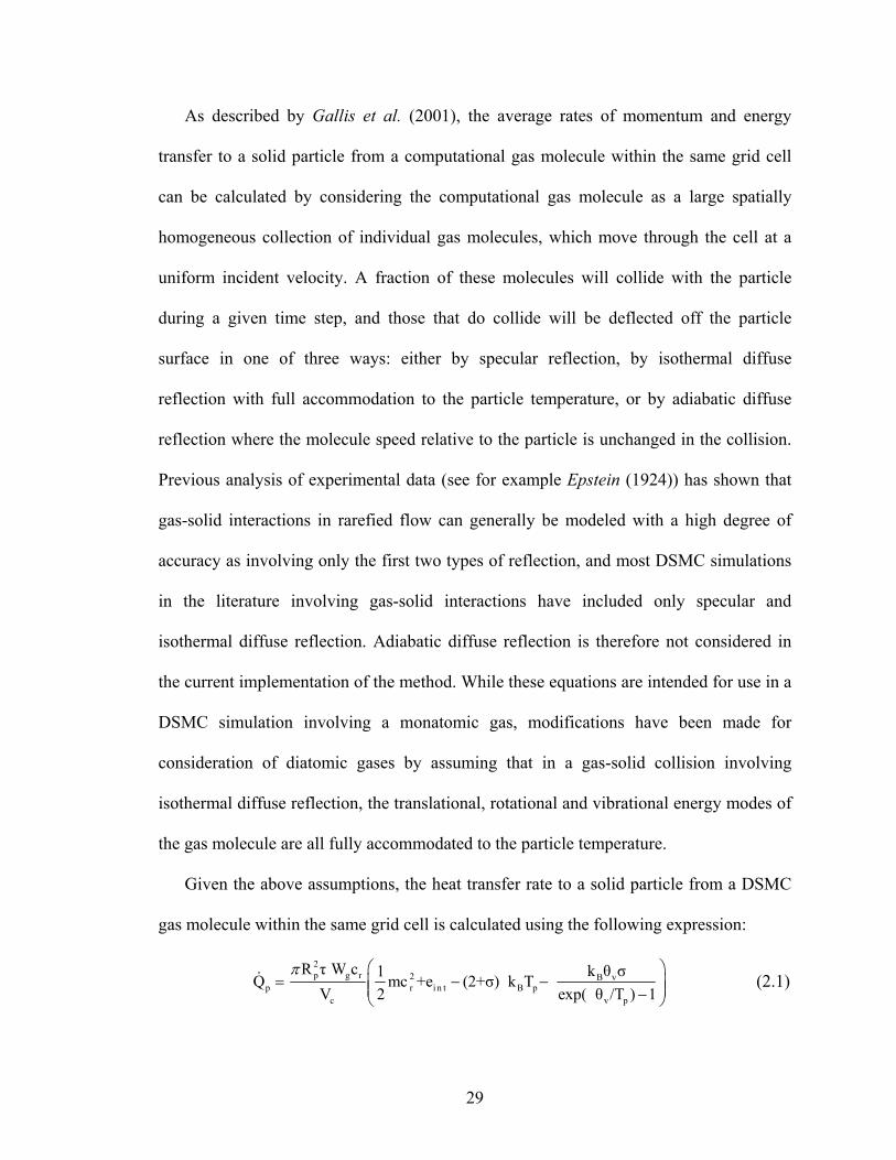
Given the above assumptions, the heat transfer rate to a solid particle from a DSMC
gas molecule within the same grid cell is calculated using the following expression:
2p g r 2 B v
p r i n t B pc v
R τ W c k θ σ1Q mc +e (2+σ) k TV 2 exp( θ /T ) 1
π ⎛ ⎞= − −⎜ ⎟⎜ ⎟−⎝ ⎠p
(2.1)
29

Here Rp is the radius of the solid particle, Vc is the cell volume, τ is the thermal
accommodation coefficient for the particle, Wg is the gas molecule relative weight (the
number of real molecules represented by each computational gas molecule), cr is the
relative speed of the computational molecule with respect to the particle, m is the mass of
an individual gas molecule, and eint is the total internal energy (including rotational and
vibrational modes) of the computational molecule. Additionally, kB is Boltzmann’s
constant, Tp is the particle temperature, θv is the characteristic temperature of vibration
for the gas species, and σ is a dimensionless parameter set to equal one for a diatomic gas
or zero for a monatomic gas. Under the assumption that the vast majority of the energy
lost by a gas molecule during the collision process is transferred to the particle as thermal
energy, Eq. (2.1) can be used to compute the rate of heat transfer to the particle. The
corresponding force on the particle can be given as
Fp = 2p g
r Bc
R W τmc + 2 m k TV 3
ππ⎛
p⎞
⎜ ⎟⎝ ⎠
ur (2.2)
where ur is the relative velocity of the gas molecule with respect to the particle.
Note that the thermal accommodation coefficient τ is equal to the fraction of
interphase collisions which involve diffuse reflection, and that the remaining fraction (1-
τ) of collisions involves specular reflection. Also note that no consideration is made for
the effect of collisions between reflected molecules and incident molecules surrounding
the particle, so that the gas is assumed to be locally free-molecular for the calculation of
gas-particle interactions. As a result, this method neglects the potentially significant
variation in the gas velocity distribution over the particle surface expected when the
30

particle Knudsen number – the ratio of the freestream mean free path to the particle
diameter – is of order one or smaller.
As implemented in the code, the temperature and velocity of a particle are updated
during each time step by summing over the force and heat transfer contributions of every
computational gas molecule within the same grid cell, using Eqs. (2.1) and (2.2). The
resulting change in particle temperature is then calculated as the total heat transfer rate
multiplied by a factor ∆t/(mpcs), where ∆t is the size of the time step, mp is the particle
mass, and cs is the specific heat of the particle. Likewise, the change in particle velocity is
equal to the total force multiplied by ∆t/mp. Particle positions are then varied during each
time step by the vector product of ∆t and the average of initial and final velocities.
2.2 Application to a free expansion flow
To evaluate the overall accuracy of the numerical procedures described above, and to
ensure proper implementation in MONACO, a series of simulations are performed for
comparison with the results of an experimental study by Israel and Friedlander (1967)
which examines the aerodynamic focusing of aerosol beams through a vacuum. As
described by the authors, a particle-air mixture is ejected through a convergent nozzle
into a near-vacuum, with a small plate oriented normal to the nozzle axis placed some
distance downstream. In the nearfield free expansion region just beyond the nozzle exit,
the gas and particles interact in such a way that the particle trajectories, and therefore the
size of the particle beam, will depend on the source pressure po of the gas. The solid
angle δ of the beam is determined by measuring the area of the particle deposition on the
plate.
31

2.2.1 Evaluation of the two phase simulation method
As discovered by Israel and Friedlander, there is a particular source pressure, or
range of pressures, for which the value of δ is minimized. This is explained by the
following logic: As the gas freely expands in the region just beyond the nozzle exit, a
force is exerted on the particles in the outward radial direction, following the streamlines
of the gas. This outward force counters the initially inward-directed momentum of the
particles as they tend, due to inertia, to follow straight trajectories after exiting through
the convergent nozzle. At relatively high values of po, the influence of the gas outweighs
the influence of particle inertia, so that the particles are redirected by the gas into outward
radial trajectories, and the particle-gas interaction acts to increase the value of δ.
Likewise, at very low source pressures, the gas exerts little influence on the particles in
the near-field expansion region, and the particles tend to follow relatively straight
trajectories that pass through the central axis, then continue in radially outward directions
further downstream. Thus, at some intermediate po value, the countering influences of
drag and particle inertia will cancel each other out. Particle trajectories will then be
nearly parallel to the nozzle axis in the far-field plume region, and the size of the particle
beam will be minimized.
Experiments were conducted by Israel and Friedlander over a wide range of source
pressures, using three different sizes of spherical latex particles. As the largest particles
were found to have Knudsen numbers too small for accurate modeling using the
equations discussed above, and as particle depositions corresponding to the smallest
particle size were found in the experiment to show a less conclusive trend, only the
32

medium-sized particles – of diameter 0.365 µm – are considered in the simulations used
for comparison with experimental results. While these experiments only allow for direct
validation of the Gallis momentum transfer formulation as implemented in the current
code, the existence of a source pressure for which the beam size is minimized – as well as
agreement in the value of this pressure – can provide convincing evidence of the overall
accuracy and functionality of the code.
Figure 2.1. Grid geometry and boundary conditions.
Due to both the enormous computational expense of DSMC simulations involving
regions of relatively high density gas, and the fact that the DSMC method often requires
massive computation time to produce accurate flow rates in simulations involving very
low Mach numbers, the grid domain in all simulations described here includes only the
comparatively high Mach number (M≥0.2), low density section of the nozzle within 1
mm of the throat. Following the description of nozzle geometry in the experimental
paper, the inflow boundary then corresponds to a local nozzle radius of 0.2352 mm, with
a specularly reflecting wall converging at a constant angle of 3.25 degrees toward a throat
of radius 0.0785 mm. Additional boundary conditions imposed in the simulations include
a specularly reflecting wall along the plane of the nozzle exit, outflow boundaries parallel
and normal to the central axis which runs through the nozzle, and a symmetry boundary
along this axis. Grid dimensions and boundary types are shown in Fig. (2.1).
33

Although gas properties within the nozzle could, in theory, be more accurately
modeled through the use of diffusely reflecting – rather than specular – wall boundaries,
the resulting boundary layer along the nozzle wall would be very thin relative to the size
of the grid. As large gas property gradients are expected within this boundary layer,
accurate simulation would require a reduction in cell size along the nozzle wall, and the
computational expense of each simulation would increase considerably. Moreover, it can
be assumed that the existence of a thin boundary layer along the nozzle wall would have
little if any influence on particle properties in the farfield plume region.
Not counting the region within the nozzle, the grid used in all simulations extends an
axial distance of 6mm and a radial distance of 0.8 mm, comprising a total of about 31,600
cells. As described in the experimental paper, a skimmer is used to aid in evacuating the
gas in the region just beyond the nozzle exit, while not interfering with particle
trajectories in the beam. Because insufficient details are given of the skimmer geometry,
it is neglected in the boundary conditions of the simulations described here. Moreover,
the skimmer is used in the experiments only to better facilitate the desired far-field
vacuum condition, so it should not in principle need to be considered in simulations
where this condition can be prescribed through the use of DSMC outflow boundaries.
The gas here is a mixture of N2 and O2, with mass fractions of 0.79 and 0.21
respectively. For all cases considered, the source temperature is 298 K, and assumptions
of one-dimensional isentropic flow within the nozzle give an inflow Mach number of
0.20, with a corresponding gas static temperature of 295.63 K and axial gas velocity of
69.176 m/s. Note that all of these values are independent of the source pressure. The
inflow static pressure is determined using the isentropic relation between the inflow and
34

source temperatures and pressures. The gas number density along the inflow boundary is
then calculated from the inflow temperature and pressure, using the ideal gas law.
For simplicity, and with likely little influence on the simulation results, the radial
component of the inflow gas velocity is set to zero. Following an assumption that the
particles experience very little temperature variation through the low Mach number
section of the nozzle not included in the grid domain, the inflow particle temperature is
set to equal the source temperature of 298 K. Further, the axial component of the inflow
particle velocity is assumed to equal that of the gas, and the corresponding particle radial
velocity is calculated so that, within the plane of symmetry defined by the grid, all
particle velocity vectors along the inflow boundary are parallel to the wall.
This last approximation, while greatly oversimplifying the particle trajectories at the
inflow boundary, can be assumed to allow for accurate representation of the particle
properties within the plume. As evidence of the validity of this assumption, consider the
following two cases: First, when the source pressure is relatively high, the particles tend
to follow the gas streamlines throughout the nozzle, so that any significant difference
between the local gas and particle radial velocity components at the inflow boundary will
quickly disappear a short distance downstream. Second, if the source pressure is very
low, then the particles will not follow the streamlines within the nozzle, and particles will
tend to impact the walls and pass through the central axis in a manner that seems
physically consistent with the inflow condition described here. For comparison, a few
simulations are repeated using values of the particle inflow radial velocity component
that scale with distance from the central axis, such that particle trajectories along the
inflow boundary are parallel to the nozzle wall only at the point where the inflow and
35

wall boundaries meet. As described below, these simulations result in very small beam
sizes for low source pressures, as the lack of particle-wall collisions allows for a very
small “focal point” of the beam, some distance downstream of the nozzle, where the
beam diameter approaches zero as the source pressure is reduced. While focal points
were observed in the experiments involving the largest particle size (which is not
considered here) the lack of particle-wall collisions, and the assumption that particles
follow the gas streamlines even for very low source pressures, does not reflect the
expected physical characteristics of the flow, and the results from these simulations can
be considered less valid than those for which the inflow particle velocity is constant.
Axisymmetric simulations are performed over a range of source pressures po from
14.8 mmHg to 96 mmHg, each corresponding to a po value used in the experiment. The
gas molecule relative weight Wg varies from 3×10⁸ to 6×10⁸ depending on the source
pressure, so that approximately 200,000 computational gas molecules are simultaneously
tracked through the grid. For all cases considered, the analogous relative weight Wp of
the particle phase is set to equal one, and the inflow particle mass flux mp is 0.12 kg/m2s.
This corresponds to a particle number density of about 6.1×10¹³ particles/m3 along the
inflow boundary, and a total of between 10,000 and 15,000 particles simultaneously
within the grid domain. Following experimentally determined properties for latex or
similar materials, all particles are given a specific heat of 2180 J/kg K, a material density
of 1120 kg/m3, and a thermal accommodation coefficient of 0.89.
Note that collisions between particles, as well as the effect of interphase collisions on
the gas, are not considered, so that the magnitude of mp will have no influence on any
flow properties other than particle phase fluxes and bulk densities. Of the properties
36

which are affected, all trends (for example, the shape of iso-contour lines) will still be
independent of the value of mp. As no values for particle flux or flow rate are given by
Israel and Friedlander, the value of 0.12 kg/m2s used here is chosen only so that the
number of particles tracked through the grid is large enough to allow for relatively low
statistical scatter, but not so large that excessive computational expense is required for
convergence to steady state.
Flow properties in each cell are averaged over approximately 300,000 time steps
following convergence. Figure (2.2) is included here for clarification of basic flowfield
characteristics, and shows the Mach number of the gas at an intermediate source pressure
of 34.5 mmHg. For all simulations, the particle number flux along the planar outflow
boundary is plotted in Fig. (2.3) as a function of distance r from the axis.
Ideally, the profiles shown in Fig. (2.3) would have relatively flat regions near the
central axis, followed in each case by a sharp drop-off to zero at a radial value ro that
could be interpreted as the “edge” of the particle beam. The corresponding beam solid
angle could then be calculated as δ = πro2/L2 where L = 6 mm. Unfortunately, as
displayed in the figure, the radial decay in the number flux is approximately exponential,
particularly for the lower source pressures considered. While the edge of a particle beam
could therefore be defined as the r value for which the number flux drops below some
given value, the resulting δ values would then be highly dependent on both the cutoff
value chosen and the assumption that, in all experiments for which the simulation results
are to be compared, the particle deposition was collected over approximately the same
time interval.
37
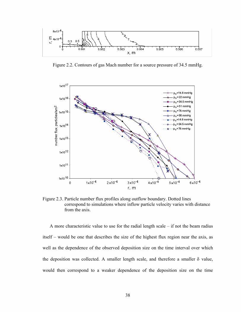
Figure 2.2. Contours of gas Mach number for a source pressure of 34.5 mmHg.
Figure 2.3. Particle number flux profiles along outflow boundary. Dotted lines
correspond to simulations where inflow particle velocity varies with distance from the axis.
A more characteristic value to use for the radial length scale – if not the beam radius
itself – would be one that describes the size of the highest flux region near the axis, as
well as the dependence of the observed deposition size on the time interval over which
the deposition was collected. A smaller length scale, and therefore a smaller δ value,
would then correspond to a weaker dependence of the deposition size on the time
38

interval, so that running the experiment for longer would do little to increase the
deposition size. Based on the observation that the outflow particle number flux scales
roughly exponentially with r for most source pressures considered, the following radial
length scale is used: For each set value of the source pressure po, f(r) = B exp(-Ar) is the
exponential trend line for the outflow particle number flux profile, where A and B are
constants determined from a least-squares fit. A larger value of A then corresponds to a
number flux distribution more closely concentrated toward the central axis. Thus, by
dimensional reasoning, the particle deposition radius ro should scale roughly with 1/A,
which can then be used as the relevant length. Finally, as the solid angle δ is proportional
to ro2, it follows that δ should scale with 1/A2. The simulation results shown in Fig. (2.3)
are used to obtain A values corresponding to each source pressure po considered, so that
the variation of δ with po can be approximated from the simulations and compared to
analogous experimental results.
Note that, in addition to the simplifying assumptions used to define boundary
conditions and other simulation parameters, a major potential problem with this
validation method is that values of A will depend on the radial distance over which the
least-squares trend line fit is performed, as well as the distribution of grid points along the
outflow boundary. This dependence is particularly large at higher source pressures, where
the outflow number flux distribution is shown in Fig. (2.3) to vary significantly from an
exponential shape. For consistency, all A values are calculated using exponential trend
lines that extend over the entire radial distance for which the outflow particle number flux
is nonzero. It can be argued that equally valid but very different values of A could be
found by performing each least-squares fit over a different set of grid points, or by
39

neglecting the points where the particle number flux is nearly zero. Subject to these
inherent problems and simplifications, it is still expected that, if the simulations
accurately model the flows considered in the experiments, the plot of po against 1/A2
from the simulation results will have the same general shape as a plot of po against δ from
the experiments.
Figures (2.4) and (2.5) show, respectively, the dependence of 1/A2 on po from the
simulations, and experimental values of δ as a function of po. A comparison of the trends
on the two plots reveals some major differences: The sharp increase in beam size at very
low source pressures, as found in the experiment, is far less pronounced in the numerical
results. The range of po values for which the beam size varies little with po is much
smaller in Fig. (2.4) than in Fig. (2.5), where this range extends from po = 34.5 mmHg
through 96 mmHg, the largest source pressure considered in the simulations.
Two very important trends are however found in both sets of results. First, in both
Figs. (2.4) and (2.5), there is a reduction in beam size as po is increased from the lowest
value (14.8 mmHg), with a consistently positive curvature that leads to a minimum beam
size, followed by an increase in beam size with source pressure as po is further increased.
Second, the po value for which the beam size is minimized is the same (34.5 mmHg) in
both figures. Furthermore, the comparatively rapid increase in beam size with po
observed on the right side of Fig. (2.4) can be attributed to the fact that, for the
corresponding simulations, the outflow number flux profiles are not very well correlated
with the exponential trend lines used to define the beam size.
40
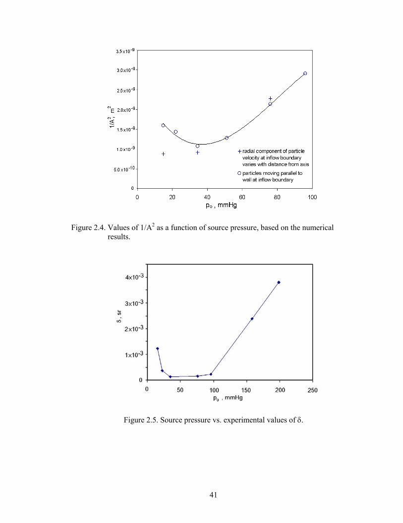
Figure 2.4. Values of 1/A2 as a function of source pressure, based on the numerical
results.
Figure 2.5. Source pressure vs. experimental values of δ.
41

Note the data points in Fig. (2.4) marked with “+” symbols, which correspond to the
simulations for which the radial component of particle velocity along the inflow
boundary is set to vary with distance from the axis. As discussed above, these simulations
should under-predict the beam size for lower source pressures, so that the trend observed
in Fig. (2.4) of a monotonic increase in beam size with po should not be thought to reflect
the overall accuracy of the simulation method.
Figure 2.6. Variation with source pressure of terminal particle velocity along the central axis.
Figure (2.6) shows the dependence on po of the average terminal particle velocity up∞
along the central axis, as measured from the simulation results at the outflow boundary 6
mm downstream from the nozzle exit plane. Because a denser gas exerts greater force on
the particles as it expands within and beyond the nozzle, the trend of increasing up∞ with
po observed in Fig. (2.6) is very much expected. Experimental measurements of up∞ give
values of roughly 200 m/s for source pressures of both 34.5 mmHg and 65 mmHg,
42

subject to errors of approximately 10 m/s. While the difference in trends between
experimental and simulation results is significant here, it should be noted that the
terminal bulk gas velocity along the axis is found numerically to exceed 700 m/s, so that,
as a fraction of the terminal gas speed, the differences in particle speed are relatively
small. Also note that the discrepancy observed in Fig. (2.6) involves only one of the two
experimental data points, and that as discussed by Israel and Friedlander (1967), the
experimental method for measuring up∞ is inherently imprecise and prone to potentially
large errors.
Subject to the assumptions and simplifications described above, the simulation results
agree well with data from the experiments. In general then, it can be assumed that both
the two phase DSMC method of Gallis et al. (2001) and the current implementation of
this method do function as expected, and allow for relatively accurate simulation of two
phase rarefied flows. Note however that only dilute particle concentrations have been
considered, as the Gallis procedures only allow for simulations of one-way coupled flow
where the influence of the particle phase on the gas can be neglected. While not explicitly
stated by Israel and Friedlander, it is assumed that particle concentrations in the
experiments are small enough that the rate of momentum transfer from the gas to the
particles is consistently much lower than the gas momentum flux, so that two-way
coupling effects are negligible and the Gallis method is appropriate for the simulation of
these flows. However, the assumption of one-way coupling is not always valid for the
SRM plume flows of interest, where the particle phase mass fraction is relatively high
and interphase momentum and energy transfer may significantly alter the properties of
the gas. A detailed numerical model for two-way coupling is therefore necessary for more
43

general simulations of rarefied particle-gas flows. One such model is introduced in
Chapter 3.
2.2.2 Additional results
Additional simulation results are provided here for the particle beam flows described
in the previous section. These results, although not usable for comparison with the
experiments, demonstrate the utility of the method while allowing for a deeper
understanding of the physical characteristics of the flows considered here.
Figure (2.7) shows the variation in the relative Mach number Mp of the particles with
respect to the surrounding gas. Mp is defined as the magnitude of the vector difference
between the particle and the gas bulk velocities, divided by the local sonic speed of the
gas. Values of Mp are plotted along the central axis for simulations at source pressures of
14.8, 34.5 and 96 mmHg. The first and last of these pressures are, respectively, the lowest
and highest po values considered in this study. The inclusion of results from these three
simulations should therefore allow for an understanding of the full range of flow
conditions. Note that points with x-coordinate values between 0 and 0.001 m are located
within the nozzle, and all other points are in the plume.
Neglecting effects of statistical scatter in the far-field plume region, the relative Mach
number is found in all three simulations to continuously increase with downstream
distance. This follows from the fact that throughout both the nozzle and plume, the gas
velocity is increasing and the gas temperature is decreasing, while the particle velocity
varies far less rapidly. To reinforce this last point, a corresponding plot of average
particle speed along the central axis is included here as Fig. (2.8).
44

Figure 2.7. Comparison of relative particle Mach numbers along the central axis for simulations at three different source pressures.
Figure 2.8. Particle speed along the central axis.
45

Figure 2.9. Drag force on particles along the central axis.
Figure 2.10. Particle Knudsen number along the central axis.
46

As discussed above in the comparison with experimental results, the particles are
shown in Fig. (2.8) to reach a near-terminal velocity within a short distance of the nozzle
exit, and the magnitude of this terminal velocity increases with the source pressure po. An
interesting trend observed in Fig. (2.8) is that the size of the near-field region of the
plume where particle acceleration is significant has little, if any, dependence on the value
of po.
Figure (2.9) shows the magnitude of the average drag force Fp on the particles along
the axis. Under steady state conditions, this force is equal to the dot product of the
particle velocity with the velocity gradient tensor, multiplied by the particle mass. Thus,
|Fp| can be thought to scale roughly with the slope of the particle speed curves plotted in
Fig. (2.9). A comparison with Fig. (2.9) then explains the general trends observed in Fig.
(2.8), most notably that the lack of variation in far-field particle velocity corresponds to a
sharp drop-off in the force exerted on the particles by the expanding gas.
Another prominent trend in Fig. (2.9) is that for all three simulations considered, the
values of |Fp| are far greatest around the nozzle exit, with a global maximum at the exit
plane. This can be explained by the following logic: At the inflow boundary, the average
particle and gas velocities are approximately equal. Thus, even though the gas density is
greatest at this boundary, the drag force should be relatively small. (The thermophoretic
force due to the gas temperature gradient may be significant here, and accounts in part for
the fact that Fp is still much greater at the inflow boundary than in the far-field region of
the plume.) As the gas expands and accelerates through the nozzle, the particle velocity
lag dramatically increases, so that |Fp| values increase greatly with downstream distance
through the nozzle. The particle velocity lag continues to grow as the gas expands beyond
47
the nozzle exit, but there is a rapid reduction in gas density that offsets the increasing
relative velocity of the gas. As a result, values of |Fp| will decrease throughout the plume.
The force exerted on the particles therefore reaches a maximum value at the nozzle exit,
beyond which the slope of the |Fp| profile changes sign. Furthermore, the requirement that
|Fp| values be relatively small within a short distance both upstream and downstream of
the nozzle exit gives rise to a sharp spike in the force profile at the exit plane, as shown in
the figure.
The variation in particle Knudsen number along the central axis is displayed in Fig.
(2.10). For all three simulations, the particles are found to be in the transition regime
within and just beyond the nozzle, and well within the free molecule regime further
downstream. Note the distinction between the particle Knudsen number, which
characterizes the effect of collisions in creating local variation in the gas properties near
the particle surface, and the Knudsen number of the flow, which characterizes the overall
influence of collisions on average properties in the gas.
All simulations used for comparison with experimental results are characterized by a
lack of significant energy transfer between the particles and gas. This is reflected in the
fact that particle temperatures are found to be nearly uniform throughout the grid domain.
In order to consider the effects of interphase energy transfer, the simulation boundary
conditions must then be changed in ways that do not reflect the flow characteristics in the
experiments. As particle temperatures are almost universally greater than the local gas
temperature in the two phase SRM plume flows of interest, a simple and desirable way to
evaluate the heat transfer formulation is to perform simulations where the particle
temperature at the inflow boundary is much greater than the local temperature of the gas,
48

and where all other parameters are unchanged from the simulations described above.
Thus, the simulations corresponding to source pressures of 14.8, 34.5, and 96 mmHg are
repeated with the inflow particle temperature increased by 100 K to 398 K.
Figure 2.11. Magnitude of the average particle heat transfer rate along the axis.
Figure (2.11) shows the variation in the magnitude of the interphase energy transfer
rate along the central axis, for all three of these simulations. While the temperature
difference between the gas and particles is found to increase continuously with
downstream distance in both the nozzle and plume, the heat transfer rate from the
particles to the gas is shown in the figure to continuously decrease. This trend can be
attributed to the reduction in gas density through the nozzle, and the far more rapid
reduction in gas density within the plume. This density effect outweighs the influence of
the growing temperature lag, so that even as the average energy transferred per interphase
collision increases with downstream distance, the decline in collision frequency results in
an overall reduction in the heat transfer rate as particles move downstream. Because the
drop-off in gas density is most prominent in the near-field region of the plume, the
49

decrease in the heat transfer rate should be greatest in this region just beyond the nozzle
exit, as is shown in Fig. (2.11).
Figure 2.12. Variation along the axis in average particle temperatures.
The average heat transfer rate to an individual particle can be expressed as
=mpQ pcsup·∇Tp, where mp is the particle mass, cs is the specific heat of the particle
material, up is the mean particle velocity, and Tp is the average particle temperature. The
gradient of Tp should then scale roughly with the magnitude of the heat transfer rate. This
trend is observed for all three simulations through a comparison of Fig. (2.11) with Fig.
(2.12), which shows the variation of average particle temperature with distance along the
axis. As displayed in Fig. (2.12), the particle temperature varies significantly through the
nozzle and the near-field plume region, then reaches a nearly constant value within a
short distance of the nozzle exit. This final value is found to be highly dependent on the
gas source pressure. Note that analogous trends for the particle speed are observed in Fig.
(2.11).
50

As shown in Eq. (2.2), the force exerted on a particle by a colliding gas molecule will
depend on the temperature of the particle. It follows that a change in particle temperature
must alter the magnitude of the average force on the particles, so that the distribution of
particle speed will also change. Figure (2.13) shows the ratio of the cell-averaged particle
speed cp in all three simulations to a corresponding particle speed cpo in simulations
where the inflow particle temperature is set to the original value of 298 K. This ratio
(cp/cpo) is plotted over 100 points along the central axis.
Figure 2.13. Fractional change in average particle speed associated with an increase in particle temperature.
From Eq. (2.2), it is expected that an increase in particle temperature will result in a
greater force exerted on the particles by the accelerating gas. As Tp increases, values of cp
should then increase, and the ratio (cp/cpo) should be greater than one. This is observed in
Fig. (2.13), where (with the exception of a very few points near the inflow boundary
which are not shown, and where cp/cpo is just slightly below unity) the ratio of particle
speeds is found to be consistently greater than one. In addition, the values of (cp/cpo) tend
51

to rise with downstream distance, because the force – and therefore the spatial gradient in
the particle speed – will increase with particle temperature. The considerable statistical
scatter observed in Fig. (2.13) is a consequence of the fact that even though the particle
speed is influenced by the value of Tp, this influence is relatively small, and the ratio
(cp/cpo) is consistently very close to unity.
2.3 Simulation of nonspherical particles
While experimental studies have shown that alumina (Al2O3) particles in solid rocket
exhaust flows tend to be nearly spherical, surface forces on a solidifying alumina droplet
may result in particle shapes which differ noticeably from a perfect sphere. [Reed and
Calia (1993), Gosse et al. (2003)] Nonspherical particles are also prominent in similar
flows involving a two phase free expansion, including liquid propellant rocket plume
flows and spacecraft fuel venting flows. In particular, ice particles from condensed water
vapor in rocket exhausts, and soot particles associated with heterogeneous combustion in
both solid and liquid propellant rockets, may have highly nonspherical shapes. [Kassal
(1974), Simmons (2000)]
Following the assumptions discussed in Section 2.1 on which the method of Gallis et
al. (2001) is based, these nonspherical particles can also be considered through the
following analysis. First, a few additional assumptions must be made for any
nonspherical particle: The particle is assumed to have a convex shape, which is defined
here as a shape bounded by a surface through which no straight line can pass more than
twice. In addition, the particle is assumed to move through the gas with an isotropic
distribution of orientations relative to any fixed coordinate system, so that no one
52

orientation is more likely than any other. While this implies that a nonspherical particle
must be rotating, it is further assumed that any rotation effects – particle angular
momentum, the side force due to an asymmetric surface pressure distribution, rotation-
induced time variation in interphase momentum and heat transfer, etc. – are relatively
small and can be neglected. These assumptions are expected to be valid over most
relevant flow regimes for a variety of particle types. Note however that particle rotation
effects will be considered in more detail in Section 2.4, where some of these assumptions
are relaxed.
Subject to the above assumptions, the convective heat transfer rate between a solid
particle and the surrounding gas will depend on the particle shape only through the value
of the average collision cross section for interphase collisions, given here as σ.
Furthermore, the average momentum transfer rate will depend on the particle shape only
through the value of σ and through the distribution function of the collision angle θ. Here
θ is defined as the angle between the relative velocity ur = um – up of an incident gas
molecule and the inward normal vector at the collision point on the particle surface,
where um and up are the velocities of the gas molecule and particle, respectively, in a
fixed reference frame. Thus, if the particle shape dependence for σ and the distribution
function f(θ) can be found, then subject to the assumptions described above, the influence
of particle shape on the rates of interphase momentum and energy transfer can be
determined.
53

2.3.1 Collision angle distribution function
First consider the dependence of f(θ) on the particle shape. For an arbitrary convex
particle, let the particle surface be divided into a large number N of flat surface elements,
each of area ∂A. Now assume that a gas molecule collides with the particle on a
particular surface element i. If all orientations of the particle for which this collision may
occur are equally likely, then the relative velocity vector of the incident molecule has an
isotropic distribution over θ∈[0,π/2]. This vector will be contained within a solid angle
element of size sinθdθdφ, where φ is the azimuthal angle relative to some reference
direction in the plane of the surface element. Therefore f(θ) must be proportional to the
size of the solid angle, so that f(θ)∝sinθ.
Now, if we remove the requirement that the collision occurs on the surface element i,
and only assume that a collision does occur somewhere on the particle surface, then the
probability that the collision point will be located on element i must be proportional to
the projected area of this element in the direction of the relative velocity vector ur. Thus
f(θ) is proportional to this projected area ∂Acosθ, so that f(θ)∝cosθ. By the above
arguments, f(θ) must then be proportional to sinθcosθ. Applying a trigonometric identity
and the normalization condition , we find that /2
0(θ) θ = 1f d
π
∫
f(θ) = sin2θ. (2.3)
As this distribution function is valid for any surface element, it must also be valid for the
particle as a whole. Note that f(θ) will have no dependence on the particle shape, so long
as the above assumptions are valid.
54
2.3.2 Average collision cross section
Next consider the particle shape dependence of the average collision cross section σ.
As above, assume that the particle surface is made up of a large number N of flat surface
elements, each with area ∂A. Now define θi as the angle between the inward normal
vector on a given element i and the relative velocity vector ur of an incident gas
molecule. Under the assumption that the gas molecule is much smaller than the particle,
the instantaneous collision cross section σ’ will be the sum of the projected areas of all
exposed faces:
σ’ (2.4) N
1
A maxcosθ ,0ii=
= ∂∑
The average collision cross section σ can then be approximated as the average of a
large number M of σ’ values, each of which corresponds to a randomly chosen particle
orientation relative to ur. If θij is the value of θ on surface element i for the jth realization
of σ’, then σ can be given by
M N
M 1 1
1lim A maxcosθ ,0M
σ ijj i→∞= =
= ∂∑∑
N M
M1 1
1A lim maxcosθ ,0M ij
i j→∞= =
⎛ ⎞= ∂⎜ ⎟
⎝ ⎠∑ ∑
( )N
01
A (θ ) maxcosθ ,0 θi ii
g dπ
=
= ∂∑ ∫ i (2.5)
Here g(θi) is the distribution function of θi for a collision which may occur anywhere on
the particle surface. From the solid angle argument used in the derivation of Eq. (2.3), it
can be shown that g(θi) ∝ sinθi if the particle has no preferred orientation relative to ur.
55

Applying the normalization condition , we find that g(θi i0(θ ) θ = 1g d
π
∫ i) = ½ sinθi for
θi∈[0,π], so = ¼. If the total surface area of the particle is
A
0(θ )maxcosθ ,0 θi ig
π
∫ id
s = ∂A then substitution into Eq. (2.5) gives the final result that σ = ¼ AN
1i=∑ s. Thus, for a
convex particle of arbitrary shape, the average collision cross section will be one fourth
of the particle surface area.
2.3.3 Effective particle size and density
As f(θ) has no particle shape dependence and σ depends only on the particle surface
area, then subject to the assumptions discussed above, any convex particle can be
modeled as a spherical particle of the same surface area for calculations of interphase
momentum and energy transfer. Following a standard convention [Crowe et al. (1998)]
let the particle shape be characterized by a shape factor ψ ≡ Ao/As , where Ao is the
surface area of a sphere with the same volume as the particle. Define Ro as the radius of
this same sphere, which for most particle shapes will be comparable to one-half of some
characteristic average particle length. The effective particle radius Rp, for use in
momentum and energy transfer calculations, can then be determined from known values
of ψ and Ro through the following relation:
Rp = Roψ - 1/2 (2.6)
As Rp ≥ Ro it follows that a convex nonspherical particle in locally free-molecular
flow will behave like a spherical particle of equal mass but greater volume. Thus, the
larger effective radius for a nonspherical particle will be accompanied by a reduction in
56

the effective particle density. If the particle mass mp is calculated as mp=4/3πρpRp3 then
the effective particle density ρp can be found through the relation ρp = ρoψ3/2, where ρo is
the actual density of the particle material.
Through this analysis, the solid particle model of Gallis et al. (2001), as well as a
two-way coupling method discussed in the following section, can be extended and
applied to a variety of nonspherical particles. While the analysis is not strictly valid for
particles with highly complicated non-convex shapes, such as soot agglomerates, it is
thought that this can provide at least a first-order approximation for the properties of such
particles when included in a simulation.
2.4 Extension to rotating particles
The procedures described in Section 2.1 may be further extended for consideration of
rotating particles in a locally free-molecular nonequilibrium gas. Following a discussion
on the relevance of particle rotation to the plume flows of interest, a series of equations
are derived to compute the net force, heat transfer, and moment on a rotating sphere for
an arbitrary gas velocity distribution. Procedures are then presented for these equations to
be used as part of a numerical scheme for the simulation of two phase rarefied flows.
2.4.1 The potential importance of particle rotation
Despite the long history of SRM plume modeling efforts described in Chapter 1, little
study has been devoted to the effects of Al2O3 particle rotation in the flow regimes
common to rocket exhaust plumes, and rotation has generally been neglected in plume
modeling and analysis. In order to understand and quantify the influence of particle
57

rotation on various flow properties, the mechanisms by which particles in the plume
develop angular momentum must first be considered.
As discussed in Section 1.2, liquid Al2O3 droplets are continually formed during the
combustion process inside an SRM, with a bimodal size distribution concentrated around
diameters of roughly 1 µm and 100 µm. [Salita (1991)] The droplets are then accelerated
through the rocket nozzle, where they may encounter several different phenomena that
tend to contribute angular momentum. First, smaller droplets are accelerated by the
expanding gas far more rapidly than the larger droplets, so that droplets of different sizes
develop widely varying velocities. The high number density and considerable relative
velocities between droplets of different sizes allow for a large number of collisions,
which results in the coalescence of droplets into larger agglomerates. These agglomerates
in turn tend to rotate due to the off-center nature of most coalescing collisions. [Vasenin
et al. (1995)] At the same time, larger droplets tend to break apart within the nozzle due
to collisions or surface stresses imposed by the accelerating gas, and these breakup
processes may impose significant angular momentum on the resulting droplet products.
Within the subsonic converging nozzle region, larger droplets may diverge
considerably from gas streamlines and accumulate in the boundary layers along the
nozzle wall, where large transverse gradients in the bulk gas velocity can also induce
rotation. [Crowe et al. (1998)] As the droplets cool and solidify into solid particles,
inelastic collisions between particles may contribute to rotation as well. Turbulent and
acoustic fluctuations in the gas can intensify many of these rotation mechanisms.
As particles exiting the nozzle in an SRM exhaust flow may have large angular
velocities, a question arises regarding how rotation affects particle properties within the
58

plume. Due to the potentially nonequilibrium velocity distribution and locally free-
molecular nature of the gas surrounding these particles, existing continuum-based
correlations for the force and moment on a rotating sphere are not generally valid. The
accurate simulation of high altitude SRM plume flows involving rotating particles may
therefore require the use of a gas kinetics-based approach.
Over the past several decades, a number of authors have studied various properties
associated with the rotation of solid bodies within a free-molecular equilibrium gas.
Epstein (1924) derived the moment imparted on a rotating sphere, subject to several
constraints including a lack of translational motion. Wang (1972) determined the drag
and lift coefficients for a rotating sphere, and showed that the direction of the transverse
“lift” force is opposite that of the Magnus force for continuum flow. Ivanov and Yanshin
(1980) derived force and moment equations for various bodies of revolution. While all of
these authors have developed closed form solutions which are applicable to the general
flow regimes of interest, the formulas they provide are limited by the assumption of
Maxwellian gas velocity distribution, and none have considered the effect of rotation on
interphase heat transfer. In addition, these formulas tend to be very complicated and
poorly suited for evaluation within a larger numerical scheme for the simulation of high-
altitude plume flows. A more appropriate set of formulas may be derived as an extension
to the force and heat transfer equations of Gallis et al. (2001) presented in Section 2.1.
2.4.2 The Green’s function approach
Equations (2.1) and (2.2) are based on Green’s functions derived by Gallis et al. for
momentum and energy transfer rates to a nonrotating solid sphere in a free-molecular
59

nonequilibrium gas. As described by these authors, the net force Fp,net and convective
heat transfer rate Qp,net on the sphere may be calculated as
p,net p r r r( ) ( )f d=∫F F u u u (2.7)
p,net p r r rQ Q ( ) ( )f d=∫ u u u (2.8)
where ur is the gas velocity in a particle-centered coordinate system, f(ur) is the gas
velocity distribution function (neglecting the influence of gas molecules reflected off the
body surface), the integration in Eqs. (2.7) and (2.8) is carried out over all velocity space,
and the symbols Fp and Qp represent Green’s functions for the force and heat transfer
rates respectively. Following the assumptions in Section 2.1, and an additional
assumption that all nonrotational modes of internal energy are unexcited, these Green
functions can be given as follows:
Fp(ur) = 2p g r B p
τR n mc + 2 m k T3
π π⎛ ⎞⎜ ⎟⎝ ⎠
ur (2.9)
2 2p r p g r r r r B p
1 1Q ( ) R τ n c mc +e (2+ ζ )k T2 2
π ⎛ −⎜⎝ ⎠
u = ⎞⎟ (2.10)
Here cr = |ur|, ζr is the number of rotational degrees of freedom for the gas, er is the mean
rotational energy per gas molecule, ng is the gas number density, and all other symbols
are as described in Section 2.1. (Note that Eqs. (2.9) and (2.10) are not true Green’s
functions in a strict mathematical sense. The term “Green’s function” is however used
here for consistency with the analysis of Gallis et al.)
60

2.4.3 Force on a rotating particle
In considering the Green’s function Fp(ur) for the force imparted by the gas on a
rotating spherical particle, first note that Fp is equal to the product of the interphase
collision frequency and the average momentum transferred to the particle per
collision. The average momentum transfer can be divided into a term due to the
momentum of incident gas molecules, a term which accounts for the average momentum
exchange during specular reflection, and a corresponding term for diffuse reflection. It
can be shown that the first term is equal to mu
2p g rR n cπ
r, the second is zero, and only the third
term may be affected by the particle angular velocity.
Next, using the velocity superposition principle, the momentum transfer due to
diffuse reflection is separated into a component independent of rotation and a component
which depends on the particle angular velocity ωp but is independent of Tp . This latter
component is the only contributor in a time-averaged sense to the force Green’s function
Frot due to rotation, and allows the Green’s function for the total force on the particle to
be computed as Fp = Fnr + Frot where the nonrotational force component Fnr is found
using Eq. (2.9).
Following the above logic, the rotational force term Frot is equal to the product of the
collision frequency for diffusely reflecting collisions and the rotational component of the
average momentum transferred during diffuse reflection. Hence
(2.11) 2rot r p g r t( )= R n c m< >−π τF u u
where ut is the tangential velocity of the particle surface at the collision point in a
particle-centered reference frame. In order to evaluate <ut> we first define two Cartesian
coordinate systems (x1, y1, z1) and (x2, y2, z2). In both coordinate systems the origin is at
61

the particle center, the z1 and z2 axes are located along a line normal to the plane
containing the vectors ur and ωp , and the y1 and y2 axes are oriented in the directions of
–ur and ωp respectively. Unit vectors along the axes can be given as
r1
r
ˆcuj =− p r
1r p
ˆc sin
uk
×=
ω φ
ω 1 1
ˆ ˆ ˆi 1j k= ×
p2
p
j =ω
ω 2 1
ˆ ˆk k= 2 2ˆ ˆ ˆi j k2= × (2.12)
where ωp = |ωp|, and φ is the angle between the x1 and x2 axes as well as between the y1
and y2 axes. Two additional angles must also be used here: θ is defined as the angle
between the outward normal vector at the collision point nc and the y1 axis, and ε is the
angle between the x1 axis and the projection of nc onto the x1-z1 plane. All angles are
shown in relation to relevant vectors in Fig. (2.14).
Figure 2.14. Angles used to determine the mean tangential velocity <ut>.
62

Based on the above definitions, the tangential particle surface velocity ut can be
determined through the following procedure. First, we express the unit vector nc in the
(x1, y1, z1) coordinate system and relate the two coordinate systems to each other:
c 1 1ˆ ˆ ˆsin cos cos sin sinn i j= θ ε + θ + θ ε 1k
2ˆ⎥
⎥
(2.13)
1 2
1
1 2
ˆ ˆcos sin 0ˆ sin cos 0ˆ ˆ0 0 1
⎡ ⎤ ⎡ ⎤φ − φ⎡ ⎤⎢ ⎥ ⎢ ⎥⎢= φ φ⎢ ⎥ ⎢ ⎥⎢⎢ ⎥ ⎢ ⎥⎢ ⎥⎣ ⎦⎢ ⎥ ⎢ ⎥⎣ ⎦ ⎣ ⎦
i i
j j
k k
(2.14)
Substitution then gives
T2
c
2
ˆsin cos cos cos sinˆcos cos sin cos sinˆsin sin
i
n 2j
k
⎡ ⎤θ ε φ+ θ φ⎡ ⎤ ⎢ ⎥⎢= θ φ− θ ε φ⎥ ⎢ ⎥⎢ ⎥ ⎢ ⎥⎢ ⎥θ ε⎣ ⎦ ⎢ ⎥⎣ ⎦
. (2.15)
From Eqs. (2.12) and (2.15) and the relation ut = ωp × (Rpnc), we find a formula for ut in
the (x2, y2, z2) coordinate system.
(2.16) (t p p 2 2ˆ ˆR sin sin sin cos cos cos sin⎡ ⎤=ω θ ε − θ ε φ+ θ φ⎣ ⎦u i )k
Next, viewing angle arguments are used to derive the following joint distribution
function for the angles θ and ε:
( ) 1, cof sπ
θ ε = θ (2.17)
where θ∈[0, π/2] and ε∈[0, 2π]. Finally, to determine <ut> we integrate over all solid
angle elements dΩ = sinθdθdε corresponding to possible directions of nc. From Eqs.
(2.12), (2.16) and (2.17) we find:
( )2 /2 p
t t p0 0r
R2, sin d d3 c
fπ π
< > = θ ε θ θ ε = − ×∫ ∫u u ω ru (2.18)
63

Substitution into Eq. (2.11) gives the Green’s function for the rotational component of the
force imparted by a locally free-molecular gas on a rotating spherical particle.
3rot r p g p r
2( )= R mn3π
τ ×F u uω (2.19)
By substituting the sum of the Eqs. (2.9) and (2.19) into Eq. (2.7), the total force on the
particle can then be determined.
2.4.4 Moment due to particle rotation
Absent any additional forces which are not associated with interphase collisions, the
rotating particle will experience a damping moment about the particle center which will
tend over time to reduce the magnitude of the angular velocity ωp. Depending on the
angle between the vector ωp and the gas bulk velocity relative to the particle, the moment
may also have a component orthogonal to ωp which tends to change the axis about which
the particle rotates. This moment can be determined using the same Green’s function
approach as above. Again, incident and specularly reflected gas molecules do not
contribute to the moment, and the average moment contribution during diffuse reflection
can be shown to depend only on the tangential velocity of the particle surface. The
Green’s function Mp(ur) for this moment can then be expressed as the product of the
collision frequency for diffuse reflection and the negative average angular momentum
about the particle center imparted on diffusely reflected gas molecules:
(2.20) 2p r p g r p c t( )= R n c m<R >π− τ ×M u n u
The term <Rpnc×ut> is evaluated using Eqs. (2.15), (2.16) and (2.17), by integrating over
θ and ε.
64

( )2 /2
p c t p c t0 0R R , sinf
π π< × > = × θ ε θ θ∫ ∫n u n u d dε
2 2p p 2
1 ˆ ˆR cos sin (3 cos )4 2
⎡ ⎤= ω − φ φ + − φ⎣ ⎦i j (2.21)
From Eqs. (2.12) and the relation r pr p
1cosc
uφ =− ⋅ω
ω , the bracketed terms in Eq. (2.21) can
be rewritten in terms of ur and ωp. Substitution into Eq. (2.20) then gives an explicit
formula for the particle moment Green’s function:
r p4p r p g r r2
r
1( )= R mn c 34 cπ
⋅⎛p
⎞τ −⎜ ⎟
⎝ ⎠
uM u u
ωω (2.22)
The total moment imposed on a rotating particle in a locally free-molecular gas flow
can be determined by multiplying Eq. (2.22) by the gas velocity distribution function f(ur)
then integrating over all velocity space.
2.4.5 Heat transfer rate
As discussed in Section 2.1, it is assumed that the translational and rotational energy
modes of a diffusely reflected gas molecule are fully accommodated to the particle
temperature. As neither energy mode will be affected during a specularly reflecting
collision, the heat transfer Green’s function must be proportional to the frequency of
diffusely reflecting collisions. For a nonrotating particle, this function will include a term
which accounts for the lost kinetic energy of an incident gas molecule, a term for the
kinetic energy gained by this molecule as it is diffusely reflected off the particle surface,
and a term for the corresponding change in the average rotational energy of the molecule.
For clarity, Eq. (2.10) may be rewritten as
65
2 2 *p r p g r r kin r r B p
1 1Q ( )= R n c mc e e k T2 2
π ⎡ ⎤⎛ ⎞τ −< >+ − ζ⎜ ⎟⎢ ⎥⎝ ⎠⎣ ⎦u (2.23)
where the three terms described above are expressed separately within the brackets, and
where < > = 2k*kine BTp is the average kinetic energy of diffusely reflected gas molecules
in a particle-fixed coordinate frame.
In the case of a rotating particle, two additional considerations must be made. First,
the average post-collision kinetic energy term < > will be greater than 2k*kine BTp, and will
depend on the local tangential velocity of the particle surface. Second, the total rate of
energy transfer from the gas to the particle is equal to the sum of the heat transfer rate and
a work term associated with the force and moment on the particle. It can be shown
through asymptotic analysis that the total energy transfer rate becomes independent of the
force if the particle is much more massive than the gas molecules, but this is not true for
the moment. Thus, in determining the heat transfer Green’s function for a rotating
particle, a term
p rQ ( )u
p r( ) ⋅M u ωp must be subtracted from the total energy transfer rate to
account for the rate at which work is performed on the particle by the gas.
To determine the average kinetic energy of a gas molecule diffusely reflected off the
rotating particle, consider a single particle surface element with outward normal unit
vector nc which moves at a tangential velocity ut. In a particle-centered reference frame,
the average kinetic energy of a gas molecule diffusely reflected off this element is found
to be
*kin B p t t
1e 2 k T m2
u u= + ⋅ . (2.24)
66

The average kinetic energy of molecules diffusely reflected off any point on the particle
surface can then be determined by integrating over all surface elements where a collision
may occur. From Eqs. (2.16), (2.17) and (2.24):
( )2 /2* * 2 2
kin kin B p p p0 0
1e e , sin d d 2k T m R 3 c8
fπ π 2os⎡ ⎤< > = θ ε θ θ ε = + ω − φ⎣ ⎦∫ ∫ (2.25)
By substituting this result into Eq. (2.23) then subtracting , we find the heat
transfer Green’s function for a rotating particle:
p r p( ) ⋅M u ω
2
r p2 2 2 2p r p g r r r B p r p p 2 2
r p
( )1 1 1Q ( )= R n c mc 2 k T e m R 32 2 8 c
π⎡ ⎤⎛ ⎞⋅⎛ ⎞τ − + ζ + + ω −⎢ ⎥⎜⎜ ⎟ ⎜ ω⎝ ⎠
⎟⎟⎢ ⎥⎝ ⎠⎣ ⎦
uu
ω (2.26)
Note from Eq. (2.26) that the rotational component of the heat transfer rate scales
with the square of the particle angular velocity, so that a greater value of ωp corresponds
to an increase in heat transfer from the gas to the particle. This property can be justified
physically by considering a single surface element in a coordinate frame which is fixed to
the local tangential surface velocity. In this coordinate frame the average kinetic energy
of diffusely reflected gas molecules will be independent of ωp, while the average kinetic
energy of incident gas molecules tends to increase as ωp2. Thus, the only effect of particle
rotation here is to increase the interphase energy transfer associated with the kinetic
energy of incident gas molecules which are involved in diffusely reflecting collisions.
In the special case where a particle which moves at the bulk velocity of a Maxwellian
simple gas, Eq. (2.8) may be integrated analytically to provide a closed form solution for
the net heat transfer rate. The gas velocity distribution function here can be written as
(2.27) 3/2 3 2 2r r r( )d = exp df π − ⎡ ⎤β −β⎣ ⎦u u u ur
67

where B gm/(2k T )β= is the inverse of the gas thermal speed scale and Tg is the equilibrium
gas temperature. By integrating the product of Eqs. (2.26) and (2.27) over all , we
find
3ru ∈
( ) ( )2 1 2 2p,net p g r B g p p p
2Q = R n 4 k T T m R3
π − ⎡ ⎤τβ + ζ − + ω⎢ ⎥⎣ ⎦ . (2.28)
From Eq. (2.22), the corresponding moment imparted on the particle by the surrounding
gas is found to be
4 1p, net p g p
4= R3
π ρ −− τβM ω . (2.29)
It follows from Eqs. (2.28) and (2.29) that the component of associated with
particle rotation is equal in magnitude to one-half the rate
p,netQ
p, net p⋅M ω at which rotational
work is performed on the particle. Thus, half of the particle rotational energy lost through
the moment is transformed into thermal energy within the particle, and the
remainder of the lost rotational energy is transferred to the gas. Also note from Eq. (2.28)
that increases with ω
p, netM
p,netQ p independent of the relation between the particle temperature
and that of the surrounding gas. Thus, in the typical case where Tp>Tg, the two bracketed
terms in Eq. (2.28) are of opposite sign. Assuming the first of these terms is greater in
magnitude than the second, we find that particle rotation tends to reduce the magnitude of
the net heat transfer rate . p,netQ
68

2.4.6 DSMC Implementation
The proposed scheme for inclusion of rotating particles in a DSMC simulation is
similar to that described in Section 2.1. Representative solid particles are tracked along
with DSMC gas molecules through a computational grid, and during each time step the
total force, moment, and heat transfer rate for each particle are determined by adding
contributions from all gas molecules which are assigned to the same cell.
The force, moment and heat transfer contributions to a particle from a single DSMC
gas molecule are computed by evaluating Eqs. (2.9), (2.19), (2.22) and (2.26) with the
number density ng replaced by the ratio of the gas numerical weight Wg to the cell
volume. Once all Ng molecules in the cell have been considered, the particle velocity,
angular velocity and temperature are altered according to the relations
gN
p p ii 1p
t∆ = ( )m
u F=
∆ ∑ gN
p p i2i 1p p
t∆ = ( )2/5 m R
M=
∆µ ∑ω
gN
p p ii 1p s
t∆T = (Q )m c =
∆ ∑ (2.30)
where the subscript “i” denotes the contribution from a single DSMC gas molecule, and µ
is the ratio of the particle moment of inertia to that of a uniform density sphere with the
same size and mass. The particle position is then updated by the product of ∆t with the
average of initial and final velocities, following an assumption that the particle
experiences uniform acceleration over the time interval ∆t.
69

Chapter III
Numerical Procedures for Two-Way Coupled Flows
3.1 Derivation of a model for two-way coupling
As discussed in Chapter 1, high altitude SRM plume flows are often characterized by
a considerable transfer of momentum and energy between the gas and solid particles,
such that the properties of each phase are significantly affected by the presence of the
other. Under these conditions, the assumption of one-way coupling in the model of Gallis
et al. (2001) is invalid, and the influence of particles on the surrounding gas must be
considered. While the procedure outlined in Section 2.1 may still be used to model the
time-variation of particle properties, additional steps must be included in the calculations
to account for potentially significant two-way coupling effects. The following analysis
provides a physical model for the effect of an interphase collision on a gas molecule, and
allows for a numerical procedure through which two-way coupling may be considered.
First, note that all assumptions discussed in Section 2.1 for the method of Gallis et al.
(2001) are again used for consideration of momentum and energy transfer from a particle
to the surrounding gas. Most importantly, the particle is assumed to be in a locally free
molecular flow, so that any influence of reflected gas molecules on an incident molecule
can be neglected during the collision process. The characteristics of the collision will
70

therefore depend only on the properties of the particle and the single gas molecule
involved in the collision. Further, all interphase collisions must involve either specular
reflection or diffuse reflection with full thermal accommodation.
3.1.1 Specular reflection
Consider the collision process between an individual gas molecule and a spherical
solid particle. As shown in Section 2.3, the collision angle θ between the initial relative
velocity vector ur and the local particle surface normal at the collision point will have a
range of [0,π/2] and a distribution function given by Eq. (2.3). Let δ represent the
deflection angle in the collision, defined as the angle between -ur and the post-collision
relative velocity vector ur* = um
*– up*, where um
* and up* are the absolute velocity vectors
of the gas molecule and the particle respectively following the collision. (The superscript
“*” is used here to denote any post-collision value.) Thus, a δ value of zero is equivalent
to the relation ur* = -ur . For a collision involving specular reflection, any given θ will
correspond to a δ value of 2θ. The distribution functions for θ and δ can then be related
by f(δ)dδ = f(θ)dθ, so that, from Eq. (2.3), the deflection angle for a specularly reflecting
collision will have the following distribution:
f(δ) = ½ sinδ for δ∈[0,π] (3.1)
Note that the azimuthal angle ε of the vector ur*, relative to a fixed direction in the
plane normal to ur , must have a uniform distribution over [0,2π]. From comparison with
the distribution function g(θi) discussed in Section 2.3, it can then be shown that Eq. (3.1)
corresponds to a total lack of directional dependence in ur*. Thus, following a specularly
71

reflecting collision, the relative velocity of the gas molecule will have a magnitude of
cr=|ur| and may be oriented with equal probability in any direction.
3.1.2 Diffuse reflection
If the collision instead involves diffuse reflection, then the collision dynamics are far
more complicated, and a more involved procedure must be used to efficiently sample the
deflection angle δ from the correct distribution function f(δ). In order to determine the
shape of f(δ), two coordinate systems must now be used: First, let a coordinate system
(x,y,z) be defined so that the origin is at the particle center, the y-axis is parallel to the
initial relative velocity vector ur , and the collision point is located on the x-y plane. For
the second coordinate system (x’,y’,z’), the origin is at the collision point, the y’-axis is
along the local surface normal, and the particle center is on the x’-y’ plane. Both
coordinate systems are shown in Fig. (3.1), as are the relevant angles described below.
Figure 3.1. Coordinate systems and angles used in the evaluation of f(δ) for diffuse reflection.
72

Next, let ϕ denote the angle between the post-collision relative velocity vector ur* and
the y’-axis, and designate as χ the azimuthal angle between the x’-axis and the projection
of ur* onto the x’-z’ plane. While specular reflection requires that ϕ = θ and χ = 0, in the
case of diffuse reflection ϕ will have a continuous distribution over [0,π/2] and χ will be
uniformly distributed over [-π,π]. Through further analysis, it can be shown that the
probability that the post-collision trajectory of a diffusely reflecting molecule will be
contained within the differential solid angle dχdϕsinϕ centered at (ϕ,χ) must be
proportional to both cosϕ and the size of the solid angle. By imposing the normalization
condition and a trigonometric identity, we find the following form for the distribution
function of ϕ:
f(ϕ) = sin(2ϕ) for ϕ ∈[0,π/2] (3.2)
The angles θ, ϕ, and χ can then be related to the total deflection angle δ by
1/ 22
2
1 (sin sin χ)cosδ (cosθ sin θ tan cos χ)1 (tan cos χ)
⎡ ⎤− ϕ= − ϕ ⎢ ⎥+ ϕ⎣ ⎦
. (3.3)
A derivation of Eq. (3.3) is provided in Appendix B.
A Monte Carlo integration method may be employed to determine the shape of the
distribution function for δ. First, a value of θ is generated by applying the inverse
cumulative distribution function method [Bird (1994)] to Eq. (2.3). Here a random
number R in [0,1] is related to the desired θ value by
R (3.4) θ θ 2
0 0sin (2θ') θ' 2 sin θ' cos θ' θ' sin θd d= = =∫ ∫
Applying the same technique to Eq. (3.2), a value for ϕ is found by setting a second
random number equal to sin2 ϕ. The azimuthal angle χ is then randomly generated with
73

uniform probability over the range [-π,π]. Once θ, ϕ, and χ are known, Eq. (3.3) is used
to calculate the corresponding value of δ. This procedure is repeated a large number of
times, and δ values are sorted into bins of finite width ∆δ. The frequency that δ values
fall within each bin is then recorded to produce a histogram that approximates the shape
of the distribution function for δ over [0,π]. The resulting shape is found to be closely
approximated by the following sixth-order polynomial:
f(δ) = 0.02042δ6 – 0.2515δ5 + 1.104δ4 – 1.903δ3 + 0.4938δ2 + 1.248δ (3.5)
As an alternate procedure, an analogy with radiation transport may be used to find an
exact closed-form solution for f(δ). Siegel and Howell (1981) derive an expression for the
scattering phase function Φ(β) for the angle β between incident and scattered radiation
from a diffusely reflecting sphere with dimensions much larger than the wavelengths of
interest. They find
Φ(β) 8 sin cos3
β β βπ
= − . (3.6)
A comparison of the above analysis with the derivation of Eq. (3.6) shows that β is
analogous to (π –δ) and f(δ) is proportional to sinδ⋅Φ(π –δ). From Eq. (3.6) and the
normalization condition it follows that 0
(δ) δ = 1f dπ
∫
f(δ) ( )(4 sin δ sin δ δ cos δ3
ππ
= + − ) . (3.7)
It can be shown that the deflection angle δ and post-collision relative speed cr* are
statistically independent in a diffusely reflecting collision, hence Eqs. (3.5) and (3.7) are
valid for any molecule-particle collision pair for which diffuse reflection is involved.
Note that a spherical particle has been used here for simplicity, but the analysis in Section
74

2.3 allows Eqs. (3.5) and (3.7) to be extended to a range of nonspherical particles. Both
the numerical solution and the polynomial approximation are shown in Fig. (3.2), along
with the equivalent distribution function for specular reflection given as Eq. (3.1). Note
that a plot of Eq. (3.7), which is not shown in the figure, is nearly identical to that of Eq.
(3.5).
Figure 3.2. Comparison of distribution functions for the deflection angle δ.
3.1.3 Two-way coupling in DSMC
The above distributions are utilized in the following procedure, which allows a solid
particle in a two phase DSMC simulation to influence the surrounding gas. We first
determine which, if any, computational gas molecules will collide with the particle during
each time step. A modification of the no time counter (NTC) method of Bird (1994) is
used to find the number Ns of computational gas molecules that are selected as potential
collision partners for the particle. The value of ns is given by
75

Ns = floor( Wp Ng πRp2 (cr)max∆t/Vc+ R) (3.8)
where the operator “floor” rounds to the nearest smaller integer; R is a random number in
[0,1]; Wp is the particle numerical weight (i.e. the number of actual solid particles
represented by each computation particle); Ng is the number of computational gas
molecules assigned to the same grid cell as the particle; Rp is the particle radius; ∆t is the
time step; Vc is the cell volume; and (cr)max is the maximum pre-collision relative speed,
over a large number of time steps, for any molecule-particle pair in this cell. Once Ns
randomly selected molecules have been chosen as potential collision partners, those that
do collide are selected with probability cr/(cr)max. It can be shown that this selection
scheme corresponds to a probability
Pcoll = πWpRp2cr∆t/Vc (3.9)
that the particle will collide with a given molecule in the cell. Due to time step limitations
inherent in DSMC, it has been found that Pcoll values are almost universally several
orders of magnitude smaller than one, so that the number of collisions per particle per
time step is usually zero and is rarely greater than one.
If a given computational gas molecule is found to collide with the particle, then the
collision is determined to involve either isothermal diffuse reflection, with a probability
equal to the particle thermal accommodation coefficient τ, or specular reflection, with
probability 1–τ. If a specularly reflecting collision takes place, then the relative speed cr
is unchanged in the collision, and the post-collision relative velocity ur* is found by
multiplying cr by a unit vector n which is sampled from an isotropic distribution. (An
efficient algorithm for calculating n is discussed by Bird (1994).) If diffuse reflection
occurs, then a value of δ is found by applying Eq. (3.3) to values of θ, ϕ, and χ
76

determined using the sampling techniques described above. Depending on the efficiency
of the random number generator, it may instead be more efficient to sample δ values
directly by applying the acceptance-rejection method to Eq. (3.7). In this procedure, a
value of δ is randomly generated with uniform probability in the interval [0,π], and a
second random number R is generated between zero and the maximum of the function
f(δ) over [0,π]. If f(δ)>R then this δ value is accepted and used in subsequent calculations.
Otherwise the δ value is rejected, and the procedure is repeated.
Next, the azimuthal angle ε of the post-collision relative velocity ur* around the initial
relative velocity vector ur is randomly generated from a uniform distribution over [0,2π].
As kinetic energy is not conserved in diffusely reflecting collisions, the post-collision
relative speed cr* cannot be assumed to equal the initial relative speed cr . Instead, a value
of cr* must be determined by applying the acceptance-rejection method to the distribution
function
f(cr*) = 2β4cr
*3exp(-β2 cr*2) (3.10)
where β = [m/(2kBTp)]½ is the inverse of the most probable thermal speed for an
equilibrium gas at the particle temperature Tp, m is the gas molecule mass, and kB is
Boltzmann’s constant. For the case of a diffusely reflected polyatomic gas molecule, the
post-collision value of the rotational energy er must also be altered. As shown by Bird
(1994), the rotational energy of a diffusely reflected diatomic molecule can be calculated
as
er = – ln(R)kBTP (3.11)
where R is a randomly generated number in (0,1]. Note that vibrational activation is
assumed here to be negligible for all flows of interest, so that the vibrational term in Eq.
77

(2.2) can be neglected and conservation of energy requires that the gas molecule
vibrational energy not be altered during an interphase collision.
Now let ur, vr, and wr be the components of ur in the global coordinate system used in
the simulation. The corresponding components of ur* can be computed from the values of
ur, vr, and wr, the pre- and post-collision relative speeds cr and cr*, and the angles δ and ε
using equations similar to those derived by Bird (1994) for binary elastic collisions. We
first define three unit vectors n, t1 and t2 such that
r / c= −n u r 1
ˆˆ
×=
×n it
| n i | 2 1= ×t t n (3.12)
where is the unit vector along the x-axis in the global coordinate system. Next, ui r* may
be given in terms of the above unit vectors as
ur* = cr
* ( )1 2cosδ sin δcos ε sin δsin ε+ +n t t (3.13)
Substitution of Eqs. (3.12) into Eq. (3.13) gives the following expressions for the
components of ur*:
2 2 ½rr r r r
r
** cu = -u cosδ+sinδ sinε(v +w )
c⎡ ⎤⎣ ⎦
r r r rr r 2 2 ½
r r r
** c sin δ(c w cosε u v sin ε)v v cosδ
c (v +w )r⎡ ⎤+
= − −⎢ ⎥⎣ ⎦
(3.14)
r r r rr r 2 2 ½
r r r
** c sin δ(c v cosε u w sin ε)w w cosδ
c (v +w )r⎡ ⎤−
= − +⎢ ⎥⎣ ⎦
Eqs. (3.14) are evaluated to find ur* if the collision involves diffuse reflection. Once
the components of ur* have been calculated for either type of collision, the absolute gas
molecule velocity is updated to a final value of um*= ur
*+ up , where up is the velocity
assigned to the solid particle. Note that the collision-induced velocity difference for the
78

particle is assumed much smaller than that of the molecule. This follows from the
previous assumption that the particle is much more massive than the particle, and allows
the true post-collision particle velocity up* to be replaced by up for the calculation of um
*.
This procedure is repeated for each representative solid particle during every time
step. It can be shown, by multiplying collision energy and momentum transfer
expressions by Eqs. (3.1), (3.7), and (3.10) then integrating over the intervals δ∈[0,π] and
cr*∈[0,∞), that the average momentum and energy imparted on a gas molecule through a
collision are equal in magnitude, respectively, to the average momentum and energy
transfer rates to the solid particle (given by Eqs. (2.1) and (2.2)) multiplied by the ratio of
the time step ∆t to the collision probability Pcoll. This property has been verified for both
specular and diffuse reflection, and confirms that the method described here is consistent
with the force and heat transfer equations of Gallis et al. (2001) In addition, and in
contrast to the one-way coupled method described in Section 2.1, the two-way coupling
procedure allows the total momentum and energy of the flow to be conserved in a time-
averaged sense.
3.2 Demonstration of momentum and energy conservation
In order to demonstrate the consistency of the two-way coupling method with the
one-way coupling procedures discussed in Section 2.1, a sample simulation is performed.
All flow properties are based on those expected along the axis and just beyond the nozzle
exit plane in the exhaust flow of a small solid propellant rocket. The simulation geometry
is simplified in order to isolate the effects of gas-particle interaction, and only a small
domain is considered to limit the computational expense. The simulation is performed on
79

a rectangular two-dimensional grid, consisting of 0.1 mm long uniform inflow and
outflow boundaries, separated on either end by 20 mm long specularly reflecting walls.
The grid geometry is shown in Fig. (3.3). As no energy or longitudinal momentum may
be transferred through the walls, it can be expected that, if the new two-way coupling
method is physically consistent, the total momentum and energy flux will be the same
over any transverse plane which passes through the grid.
Figure 3.3. Grid dimensions and boundary types.
3.2.1 Simulation parameters
The gas in this simulation is a mixture of H2, CO and N2, with inflow number
densities of 2×10²³m-3, 1×10²³ m-3 and 1×10²³ m-3 respectively. At the inflow boundary
the gas is assigned a bulk speed of 2000 m/s and a temperature of 1000K. The solid phase
consists of spherical alumina particles, of diameter 3×10⁻⁶ m and 6×10⁻⁶ m, with a mass
flow fraction of 40% divided equally between particles of either size. All particles have a
velocity of 1200 m/s and a temperature of 2200 K at the inflow boundary, with a total
particle mass flux of 13.33 kg/s-m2.
The grid is divided into 5000 square cells of length 2×10⁻⁵ m, or approximately two
mean free paths. Collisions within the gas phase are considered using the variable hard
80

sphere (VHS) model, with reference molecular diameters given by Bird (1994). The time
step size is 1.5×10⁻⁹ s and the relative weights Wg and Wp are set so that, at steady state,
about 270,000 computational gas molecules and 10,000 solid particles are contained
within the grid. This corresponds to roughly 54 computational gas molecules and 2 solid
particles per cell. Once steady state has been reached, various gas and particle properties
are evaluated, and averaging is performed over approximately 200,000 time steps.
3.2.2 Results and discussion
Simulation results are shown in Figs. (3.4), (3.5) and (3.6), based on values extracted
along a line between the centers of the inflow and outflow boundaries. Due to the
relatively small changes in the characteristics of either phase expected over the limited
grid domain, the interphase transfer of momentum and energy should be nearly constant
with downstream distance, so that most flow properties will vary linearly through the
grid. The expected linear variation is observed in Fig. (3.4), where average gas and
particle speeds are plotted against longitudinal distance from the inflow boundary. The
slower particle phase is found to accelerate at a nearly constant rate, while the faster gas
decelerates as momentum is transferred to the particles.
Figure (3.5) shows the corresponding trends in the gas and particle number densities.
Neglecting the significant statistical scatter, the particle number density is found to
decrease approximately linearly and the gas number density is found to increase linearly,
as is expected from comparison with Fig. (3.4) and considerations of mass conservation.
In Fig. (3.6) the longitudinal variations in the average particle temperature and gas
translational temperature are shown. The gas and particle temperatures are found to
81

increase and decrease respectively with downstream distance, as energy is transferred to
the gas from the higher temperature particles.
As noted in Section 3.1, the accuracy and consistency of the two-way coupling
method can be determined by verifying that momentum and energy are transferred
between the two phases at equal rates, so that the total momentum or energy transfer rate
will be the same through any transverse plane which intersects the grid domain. In order
to show this, momentum and energy transfer rates of each phase are calculated along nine
equally spaced planes. While approximations for these rates could be easily found
through algebraic manipulations of the cell-averaged velocities, densities, and
temperatures, the small size of the grid and the extreme sensitivity of flux values to
statistical scatter require that a more direct approach be used.
Figure 3.4. Longitudinal variation in average gas and particle speeds.
82

Figure 3.5. Gas and particle number densities.
Figure 3.6. Variation in gas and particle temperatures.
83

Figure 3.7. Variation in longitudinal momentum transfer rates with downstream distance.
Figure 3.8. Energy transfer rates for gas and particles.
84

The procedure used here for calculating fluxes is as follows: During every time step
for which sampling is performed, additional calculations are carried out to determine
which computational gas molecules or solid particles pass through each of the nine
planes. Values are recorded for the mass, momentum, and energy transferred through
each plane, to which the mass, longitudinal momentum, kinetic energy, and internal
energy of each of these objects is either added or subtracted, depending on the direction
in which the object passes through the plane. Resulting values are then divided by the
time step size ∆t, and averaging is performed over all sampling time steps. Each time-
averaged momentum and energy transfer value is then divided by the ratio of the
corresponding mass transfer rate to the average mass transfer rate assigned at the inflow
boundary (equal to 0.002 kg/s for the gas and 0.001333 kg/s for the particles).
Note that the last step is required to account for statistical fluctuations in the number
of objects which pass through the selected planes. This is also necessary to correct for a
slight reduction in the gas number flux with downstream distance, due to the fact that
computational gas molecules may exit the grid through the inflow boundary. The
correction is only on the order of 0.1%, but is found to significantly improve the accuracy
of results, as the values of interest will vary only slightly through the length of the grid.
The variation in longitudinal momentum transfer rates is shown in Fig. (3.7). While
different scales are used for the particles and gas, the ranges of both scales are equal, so
that trends in the two profiles can be easily compared. As expected, momentum is found
to be removed from the gas at nearly the exact rate that momentum is added to the
particle phase. Both data sets are closely approximated by linear least-squares trend lines,
85

with slopes that differ in magnitude by less than 2%. Similar trends can be found in Fig.
(3.8), which shows the variation in energy transfer rates with downstream distance.
Again, the magnitudes of linear trend lines are nearly equal, and energy is observed to be
removed from the particles at approximately the same rate that energy is added to the gas.
The small discrepancies which are observed in Figs. (3.7) and (3.8), and the local
variation in the total momentum and energy transfer rates which these discrepancies
imply, can be explained by a number of factors. First, some error may be due to the
collision selection scheme given by Eq. (3.8), as gas molecules most likely to collide with
a given particle may not be chosen as potential collision partners. This may slightly
reduce the interphase collision frequency, and is a problem inherent in the NTC method
of Bird (1994) on which the collision selection scheme is based.
A more likely error source is the fact that momentum and energy are conserved only
in a time-averaged sense, as the instantaneous momentum and energy transfer arising
from a single interphase collision is not modeled in the same manner for calculations
used to alter properties of the two different phases. This difference in collision modeling
arises from the wide disparity expected in number density between solid particles and gas
molecules, so that the interphase collision frequency for a single solid particle is likely
several orders of magnitude larger than that of a gas molecule. (For the simulation
described here, these two collision frequencies differ by a factor of about 4×10¹².)
The lack of exact momentum and energy conservation should give rise to random
walk errors, which are magnified in the results of Figs. (3.7) and (3.8) due to the extreme
numerical sensitivity of the observed trends. However, these errors are shown to be
relatively small, and are expected to further decrease when the sampling period is
86

lengthened. As the DSMC method generally requires time (or ensemble) averaging over a
large number of time steps, instantaneous momentum and energy conservation should not
be required to achieve levels of accuracy in the simulation results within the expected
statistical scatter. It can therefore be assumed that Figs. (3.7) and (3.8) do adequately
demonstrate the conservation of momentum and energy, so that the two-way coupling
method is physically consistent with the procedures for momentum and energy exchange
described in Section 2.1. The initial one-way coupling method is shown in Chapter 2 to
exhibit a relatively high degree of overall accuracy, so it follows from the above
arguments that the new method should be reasonably accurate as well.
3.3 Two-way coupling procedures for rotating particles
For the DSMC simulation of two-way coupled two phase flows involving rotating
solid particles, the two-way coupling scheme must be consistent with the Green’s
function approach outlined in Section 2.4. In this case the net momentum exchange
between a particle and the surrounding gas will include a transverse “lift” term associated
with particle rotation, and the moment, rotational work and rotation-induced heat transfer
on the particle must be included in procedures for two-way coupling.
As discussed in Section 2.4, particle rotation will have no effect on interphase
collisions involving specular reflection, and the interphase collision frequency will be
unaffected by particle rotation as well. Two-way coupling procedures involving rotating
particles will therefore be similar to those described in Section 3.1.3: First, a number Ns
of randomly selected potential collision partners are chosen for each representative
particle during each time step, where the value of Ns is calculated using Eq. (3.8). Some
87
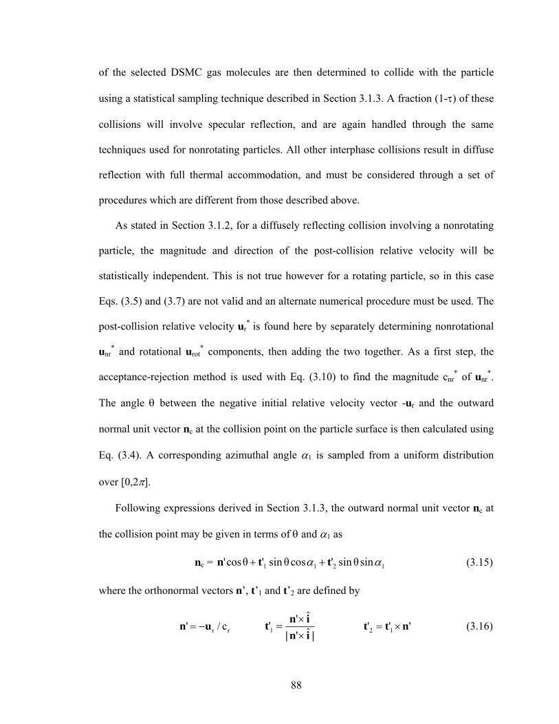
of the selected DSMC gas molecules are then determined to collide with the particle
using a statistical sampling technique described in Section 3.1.3. A fraction (1-τ) of these
collisions will involve specular reflection, and are again handled through the same
techniques used for nonrotating particles. All other interphase collisions result in diffuse
reflection with full thermal accommodation, and must be considered through a set of
procedures which are different from those described above.
As stated in Section 3.1.2, for a diffusely reflecting collision involving a nonrotating
particle, the magnitude and direction of the post-collision relative velocity will be
statistically independent. This is not true however for a rotating particle, so in this case
Eqs. (3.5) and (3.7) are not valid and an alternate numerical procedure must be used. The
post-collision relative velocity ur* is found here by separately determining nonrotational
unr* and rotational urot
* components, then adding the two together. As a first step, the
acceptance-rejection method is used with Eq. (3.10) to find the magnitude cnr* of unr
*.
The angle θ between the negative initial relative velocity vector -ur and the outward
normal unit vector nc at the collision point on the particle surface is then calculated using
Eq. (3.4). A corresponding azimuthal angle α1 is sampled from a uniform distribution
over [0,2π].
Following expressions derived in Section 3.1.3, the outward normal unit vector nc at
the collision point may be given in terms of θ and α1 as
nc = 1 1 2'cosθ ' sinθcos ' sinθsin 1α α+ +n t t (3.15)
where the orthonormal vectors n’, t’1 and t’2 are defined by
r r' /= −n u c 1
ˆ'' ˆ'×
=×
n it| n i |
2 1' ' '= ×t t n (3.16)
88

and is the unit vector along the x-axis in the global coordinate system. Substitution of
Eqs. (3.16) into Eq. (3.15) gives expressions for the three components of n
i
c.
2 2 ½c, x r r r
r
1n = u cos sin sin (v w )c 1⎡ ⎤− θ + θ +⎣ ⎦α
r r r rc, y r 2 2 ½
r r r
sin (c w cos u v sin )1n = v cosc (v w )
1 1⎡ ⎤θ +− θ −⎢ ⎥+⎣ ⎦
α α (3.17)
r r r rc, z r 2 2 ½
r r r
sin (c v cos u w sin )1n = w cos c (v w )
1 1⎡ ⎤θ −− θ +⎢ ⎥+⎣ ⎦
α α
Next, we find the angle ϕ between the vectors nc and unr* as in Section 3.1.2 by
sampling sin2ϕ from a uniform distribution over [0,1]. An azimuthal angle α2 relative to a
plane normal to the x-axis is sampled from a uniform distribution over [0,2π]. Once the
normal vector nc is known and values have been selected for ϕ, α2 and cnr*, the
nonrotational component unr* of the post-collision relative velocity is determined. This
velocity can be expressed as
unr* = cnr
* ( )c 1 2 2cos " sin cos " sin sin 2α αϕ + ϕ + ϕn t t (3.18)
where the unit vectors t”1 and t”2 are defined by
c1
c
ˆ" ˆ
×=
×n it
| n i | 2 1" " c= ×t t n (3.19)
The following expressions may be derived from Eqs. (3.18) and (3.19) to find the
components of unr*:
unr*= cnr
* 2 ½c, x c, xn cos sin sin (1 n )α2⎡ ⎤ϕ + ϕ −⎣ ⎦
vnr*= cnr
* c, z c, x c, yc, y 2 ½
c, x
sin (n cos n n sin )n cos
(1 n )α α2 2⎡ ⎤ϕ −
ϕ +⎢ ⎥−⎢ ⎥⎣ ⎦
(3.20)
89

wnr*= cnr
* c, y c, x c, zc, z 2 ½
c, x
sin (n cos n n sin )n cos
(1 n )α α2 2⎡ ⎤ϕ +
ϕ −⎢ ⎥−⎢ ⎥⎣ ⎦
Finally, the rotational component of ur* is computed as urot
* = Rp ωp×nc where Rp and ωp
are the particle radius and angular velocity respectively, and the gas molecule velocity is
reassigned to the post-collision value up+unr*+urot
*. For a diffusely reflecting collision
involving a diatomic gas molecule, the rotational energy of the molecule must also be
resampled from an equilibrium distribution at the particle temperature, as given by Eq.
(3.11).
90

Chapter IV
Additional Models for SRM Plume Simulation
4.1 Overview
While the DSMC method allows for a high degree of accuracy in the simulation of
rarefied gas flows, excessive computational cost is often cited as a major drawback. The
same is true for the two-phase model described in Chapters 2 and 3; calculations are
generally very expensive, such that any improvement in efficiency will help extend the
applicability of the method to larger-scale flows. With this in mind, a series of coupling
parameters are developed to quantitatively evaluate the importance of interphase
momentum and energy exchange for both the particles and gas. If coupling in a particular
direction and location is determined to have a negligible effect on bulk flow
characteristics, corresponding calculations for momentum or energy exchange can then
be avoided, and the overall numerical efficiency will increase.
In the current implementation, four different nondimensional parameters are
periodically evaluated in each cell within the computational grid, and time-averaged
parameter values are compared to set cutoff values to assess the significance of
interphase coupling in either direction. Derivations are provided for all parameters, and a
time-averaging scheme used to reduce memory requirements is described.
91

As discussed in Chapter 1, phase change processes involving liquid Al2O3 may have a
significant impact on a variety of SRM plume flow properties, so that the accurate
simulation of high altitude plume flows generally requires inclusion of a model for Al2O3
particle phase change. Propulsive efficiency, particle radiation, particle size distributions
and other flow characteristics are strongly dependent on the phase composition of
particles within the nozzle and plume. [Reed and Calia (1993)]
At the nozzle exit plane, the smallest particles are typically made up of some
combination of stable α and metastable γ solid phases, while the largest particles consist
entirely of liquid Al2O3. Particles of intermediate size may exist as multiphase “slush
balls” within the plume nearfield region, where finite-rate crystallization kinetics and
steam release allow for combinations of liquid, multiple solid phases, and trapped water
vapor within a single particle. [Gosse et al. (2003)] Phase composition and phase change
processes will have direct and significant effects on the refractive index and the
temperature distribution for the particles, as well as other flow characteristics which may
be of interest. Accurate plume simulation therefore requires the consideration of particle
phase change, particularly the initial crystallization process for liquid Al2O3.
A nonequilibrium particle phase change model is presented here, following procedures
of Henderson (1977), Hunter et al. (1981) and Plastinin et al. (1998) In this model, it is
assumed that homogeneous crystallization begins on the surface of a liquid droplet, at a
nucleation temperature well below that required for equilibrium melting. A
heterogeneous crystallization front then progresses toward the particle center, at a
velocity which varies as a function of the particle temperature. During this process, the
particle temperature may either increase or decrease, depending on the balance between
92

convective heat transfer and heat release during crystallization. A simple model for
particle melting is also implemented to account for any phase change effects associated
with particle-shock interactions. [Hunter et al. (1981)] Following a detailed description
of the phase change model, results from a series of subscale plume flow simulations are
used to indicate the potential importance of particle phase change, and to find appropriate
cutoff values for the determination of regions with significant interphase coupling.
4.2 Interphase coupling parameters
To reduce the computational cost of two-phase DSMC plume flow simulations,
calculations for momentum and energy exchange between the gas and particles should
ideally be made only where the flow is locally determined to involve significant
interphase coupling. A series of coupling parameters are proposed so that this
determination may be made automatically during a simulation. Coupling parameters are
periodically evaluated in each grid cell during two-phase DSMC calculations, and regions
of interphase coupling are identified through a comparison between time-averaged
parameter values and predetermined cutoff values.
Four separate coupling parameters are used here. The first parameter P1m quantifies
the importance of momentum coupling from the gas to the particles; a smaller value of
P1m indicates that the gas has less influence on the particle phase momentum flux. A
second parameter P1e relates to energy coupling from the gas to the particles, while
parameters P2m and P2e indicate the significance of momentum and energy coupling,
respectively, from the particles to the gas. These parameters are formulated with the goal
93

of minimizing the cost of parameter evaluations, while allowing for reasonable accuracy
over a wide range of flow regimes.
4.2.1 Gas-to-particle momentum coupling
The gas-to-particle momentum coupling parameter P1m is defined here to scale with
the fractional change in average particle speed, due to interphase momentum transfer,
over the mean time required for particles to move a streamwise distance L. The variable
L here represents some global characteristic length scale; for a plume flow we set L to
equal the nozzle exit diameter. Neglecting spatial variation in the particle speed
gradient pc∇ , it follows that
P1m ∝ p pp 2
p p p
1 cL cc c t c
u ∂⎛ ⎞ ∇ =⎜ ⎟ ∂⎝ ⎠i L (4.1)
where up and cp are the local bulk velocity and speed of the particle phase, respectively.
To evaluate the pct
∂∂
term, we use the fact that mppct
∂∂
is roughly equal to the product
of the average interphase collision frequency fp for a single particle and the magnitude of
the average momentum transferred per collision. (In the special case where every particle
in the cell has the same mass and velocity, it can be shown that mppct
∂∂
is equal to the dot
product of this average momentum transfer and fpup/cp.) If all particles are much larger
than gas molecules and the thermal speed of the particle phase is small, then the collision
frequency may be approximated as
fp = ¼ πngcr2Dp2 (4.2)
94

where ng is the gas number density, Dp is the average particle diameter, and cr2 is the
average gas molecule speed relative to up. If there are Ng DSMC gas molecules in the
computational cell of interest, each with some velocity um,i, then the quantity cr2 can be
given by
cr2 =g
gm,i p
i = 1
N
N
1 | |u u−∑ . (4.3)
In determining the average momentum transfer per collision, we assume that all
particles are much more massive than gas molecules, and that following an interphase
collision the gas molecule velocity is on average equal to that of the particle. As shown in
Section 3.1, the latter assumption is exact for specularly reflecting collisions, and is a
reasonably good approximation for diffusely reflecting collisions. Under these
assumptions, the average momentum transfer magnitude is roughly equal to mcr1, where
m is the mass per gas molecule, and cr1 is the magnitude of the difference between up and
the gas bulk velocity ug. The magnitude of the average force exerted by the gas on a
single particle can then be given as
mppct
∂∂
= fp m cr1 = ¼ πρg cr2 Dp2 cr1 . (4.4)
where ρg=mng is the mass density of the gas. Next, Eq. (4.4) is rearranged and substituted
into Eq.(4.1), and the average particle mass mp is approximated as 6π ρpDp
3. Ignoring a
multiplicative constant of order one, we then have the final formulation for the
momentum coupling parameter P1m:
P1m g r1 r2
2p pp
ρ c c Lρ c D
= (4.5)
95

4.2.2 Particle-to-gas momentum coupling
An expression for the parameter P2m, which characterizes momentum coupling from
the particles to the gas, is derived in a similar manner as that of P1m above. Following
Crowe et al. (1998), P2m is proportional to the magnitude of the total drag force on the
particle phase per unit volume, divided by the streamwise gas momentum flux and
nondimensionalized through multiplication by the length scale L. The streamwise gas
momentum flux is approximated here as ρgcg12, and from Eq. (4.4) the magnitude of the
force per unit volume is ¼π ρgcr2Dp2cr1np where np is the particle number density and cg1
is the bulk gas speed. Neglecting a constant of order one, the parameter P2m may then be
defined by
P2m = npDp2L r1 r2
2g1
c cc
. (4.6)
In comparing Eqs. (4.5) and (4.6), note that an identical formulation for P1m could be
found by substituting an approximate particle momentum flux mpnpcp2 for the gas
momentum flux in the derivation of P2m. The above derivation for Eq. (4.5) is used only
to show the physical significance of this parameter.
4.2.3 Gas-to-particle energy coupling
The definition of the parameter P1e for energy coupling from the gas to the particles is
analogous to that of P1m: Here P1e scales with the fractional change in average particle
temperature Tp over the time required for particles to travel a streamwise distance L.
P1e ∝ p pp
p p p
1 TL TT c t c T
u ∂⎛ ⎞ ∇ =⎜ ⎟ ∂⎝ ⎠i
p
L (4.7)
96

The time-derivative of Tp is related to the average heat transfer rate pQ per particle by
pp s p
TQ c mt
∂=
∂ where cs is the particle specific heat. Approximating mp as
6π ρpDp
3, we
then have
P1e ∝ p3
p pp p s
6 Q Lρ D c c Tπ
⎛ ⎞⎜ ⎟⎜ ⎟⎝ ⎠
. (4.8)
Note that pQ is equal to the product of the interphase collision frequency fp and the
average heat transfer per collision. To evaluate the latter term, a few initial assumptions
are used: First, we assume that the interphase heat transfer process is dominated by the
exchange of gas translational energy. It is also assumed that the ratio of |up–ug| to the
local sonic speed of the gas (the average particle Mach number) is much less than one.
Under such conditions the mean translational energy of a colliding gas molecule in a
particle-centered coordinate system can be approximated as 2r3
2
3m c The variable cr3 is
defined here as the root-mean-squared gas molecule speed relative to the bulk particle
velocity up, and may be calculated as
cr3 =
1/2g
2m,i p
g i = 1
N
N
1 | |u u⎛ ⎞⎜ −⎜⎝ ⎠
∑ ⎟⎟
(4.9)
If the collision involves diffuse reflection with full thermal accommodation to the
particle temperature, then the average post-collision translational energy will be 2kBTp.
Otherwise specular reflection is assumed, and the gas molecule will retain its initial
translational energy relative to the particle. From the above approximations, it follows
that
97

pQ = 6π ngcr2Dp
2 τ ( )2B pr3m c 3 k T− . (4.10)
By definition, all coupling parameters here must be greater than or equal to zero, so the
absolute value of pQ is used in the equation for P1e. Substitution into Eq. (4.8) then gives
the following result:
P1e = g 2r2r3
p p p s p
ρ 3k TcL τ cD c ρ c T m
− B p (4.11)
While Eq. (4.11) has been derived for a flow in which the average particle Mach
number is low and gas internal energy transfer is negligible during interphase collisions,
this parameter should be able to accurately characterize energy coupling over a very wide
range of flow regimes. If, for example, the parameter were derived under the assumption
that the particles move hypersonically with respect to the gas, the coefficient 3 in Eq.
(4.11) would be replaced by 4, and all other terms would be identical. Moreover, this last
term becomes negligible in comparison with as the relative Mach number increases,
so that Eq. (4.11) should be equally valid at the high and low Mach number limits.
2r3c
4.2.4 Particle-to-gas energy coupling
The final coupling parameter P2e, which determines the importance of energy coupling
from the particle phase to the gas, has a similar definition to that of P2m. Again following
Crowe et al. (1998), P2e is proportional to the interphase energy transfer rate per unit
volume, and inversely proportional to the streamwise energy flux of the gas Φ
E
g. In
determining the energy transfer rate, we neglect particle rotation effects and assume that
all particles are much more massive than gas molecules. It follows from these
98

assumptions that =E pQ np, so nondimensionalization by the length scale L gives the
relation P2e∝ pQ npL/Φg.
Next, pQ is given by Eq.(4.10), and the energy flux Φg is approximated as the product
of the streamwise gas number flux and the average energy per molecule. For simplicity
we consider the special case of a monatomic simple gas, where the latter term will equal
½mg2g2c and Φg ≈ ½ρg
2g1 g2c c . Here the variable cg2 represents the root-mean-squared gas
molecule velocity, and may be calculated as
cg2 =
1/2g
m,i m,ig i = 1
N
N
1u u
⎛ ⎞⎜ ⋅⎜⎝ ⎠
∑ ⎟⎟
. (4.12)
Neglecting a coefficient of order one, substitution into the above relation for P2e gives the
formula
P2e = npL Dp2 B p2r2
r32g1 g2 g
3k Tc τ cc c m
− . (4.13)
4.2.5 Implementation in DSMC
As implemented in the DSMC code MONACO for two-phase flow simulations, all
four coupling parameters are periodically evaluated at each cell within the computational
grid. For the local determination of interphase coupling, a few additional symbols are
required: Let C1 represent a user-defined cutoff value for momentum and energy coupling
from the gas to the particle phase, and define C2 as the equivalent value for coupling from
the particles to the gas. If maxP1m,P1e≥C1 then a parameter Ψ1 is set to equal one;
otherwise Ψ1 will equal zero. A similar parameter Ψ2 will be one if maxP2m,P2e≥C2 or
99

zero if maxP2m,P2e<C2. Next, define <Ψ1> and <Ψ2> as the average of a large number
of evaluations of Ψ1 and Ψ2, respectively, in a given cell. In the case of a steady flow
simulation, these averages are taken over all Ψ1 and Ψ2 values calculated for the cell
following the attainment of steady state conditions.
The values of <Ψ1> and <Ψ2> are then used to determine the importance of coupling.
At any given cell, interphase momentum and energy transfer are assumed to significantly
affect particle properties only if <Ψ1> ≥ ½ . (This is equivalent to the condition that
maxP1m,P1e≥C1 is satisfied at least 50% of the time.) Various properties of particles in
the cell are therefore altered due to particle-gas interaction only if this condition is met.
Otherwise all related calculations are avoided, and numerical efficiency is improved
through a reduction in the total number of operations. Similarly, calculations described in
Chapter 3 for use in modifying local gas phase properties are performed only if <Ψ2> ≥½.
The procedure described here is expected to significantly reduce the overall
computational cost of a variety of two-phase DSMC simulations. This is particularly true
for the high altitude SRM plume flows of interest, where interphase coupling in either
direction may be important only within a small fraction of the flowfield under
consideration. The reduction in total simulation time associated with this procedure will
be considered for a representative plume flow in Section 4.4.
4.3 Particle phase change
As discussed in Chapter 1, the phase composition of an individual particle within an
SRM plume flow is typically a strong function of particle size, position in the plume,
nozzle geometry and several other factors. Phase change processes will in turn influence
100

the particle temperature, as well as that of the surrounding gas, and may greatly affect
radiative properties throughout the plume. Several previous studies involving SRM
exhaust flow simulations have included consideration of the nonequilibrium phase
change processes typical to such flows. [Reed and Calia (1993), Henderson (1977)]
However, little effort has been devoted to the detailed characterization of particle phase
composition in high altitude plume flows, where the flow around an individual particle is
locally free-molecular and gas-particle interactions must be considered through a kinetic
theory based approach.
Following the model of Hunter et al. (1981) we consider only the dominant
crystallization process involving formation of the metastable γ phase, and neglect the γ-
to-α transition which typically occurs among smaller particles in the nearfield plume
region. The omission of a secondary phase change model is justified by both a lack of
experimental data and an assumption that the γ-to-α transition has a relatively small
effect on most flowfield properties of interest. However, any reduction in simulation
accuracy associated with this omission is corrected in part by the fact that the value used
here for the latent heat of fusion (hf = 1.07×10⁶ J/kg) accounts for the full transition of
particle material from liquid alumina to the stable α phase.
The standard model for crystallization kinetics in Al2O3 particles involves an
assumption that the phase change process is initiated only after a spherical liquid droplet
has supercooled to a nucleation temperature Tf significantly below the equilibrium
melting temperature Tm. Once this occurs, nucleation takes place uniformly over the
outer surface of the particle, and a heterogeneous crystallization front then progresses
101

toward the particle center at a rate given by
c1m p
p
cnAdr = (T T )dt R
− − (4.14)
where Tp and Rp are the particle temperature and radius respectively, r1 is the ratio of the
crystallization front radius to Rp, and Ac and nc are constants with Ac = 2.7×10⁻⁶ ms-1K-1.8
and nc = 1.8 as given by Plastinin et al. (1996) This variation in r1 in turn affects the
particle temperature through the energy balance equation
p 2 1s p p f p 1
dT drc m =Q 3 h m rdt dt
− . (4.15)
As currently implemented, the relation between the interphase heat transfer rate pQ and
the temporal variation in particle temperature is divided into three separate cases:
solidification, melting, and constant-phase heating or cooling. First, if Tp < Tf and r1 = 1,
or if Tp < Tm and r1∈(0,1), then the particle is determined to be in the process of
solidification, and r1 is updated according to Eq. (4.14). The temperature change ∆Tp is
then given by
( )p 3fp
s p s
Q t hT = rc m c
∆∆ − ∆ 1 (4.16)
where ∆(r13) is the variation in r1
3 during the time step of length ∆t. This case must be
considered for all particles throughout the grid domain, even in regions where gas-to-
particle coupling is neglected.
The relatively large local ∆t values which can be encountered for solidifying particles
within uncoupled regions may produce significant discretization errors in ∆Tp, such that
Tp can exceed the melting temperature Tm during the crystallization process. To avoid
this possibility, a variable Ns is set to equal the smallest integer for which Ns >
102

50×∆Tp/Tm. If Ns > 1 then the initial values of Tp and r1 are reassigned to the particle, the
time step is divided into Ns intervals of length ∆t/ Ns, and the above procedure is
iteratively repeated Ns times to find the final values of Tp and r1.
If Tp ≥ Tm, r1 < 1 and pQ > 0, then the particle is in the process of melting. In this case
we assume that Tp is held constant and all thermal energy transferred to the particle is
used in the phase transition. Note that for a melting particle, the normalized
crystallization front radius r1 does not physically represent a phase transition surface, but
is used instead to record the cube-root of the liquid volume fraction. The current
implementation enforces energy conservation by allowing for the special case when, in a
single time step, the last solid material in the particle melts and the remaining collision
energy is used to increase the particle temperature. Following Hunter et al. (1981) the
normalized front radius is first updated according to Eq.(4.16), where ∆Tp is set equal to
zero. If the resulting r1 value is greater than one, then the particle temperature is
increased by
( 3fp 1
s
h∆T = r 1c )− (4.17)
after which r1 is set to equal one. In the last case, where the particle is neither solidifying
nor melting, the temperature is varied as
pp
s p
Q ∆t∆T =
c m (4.18)
following the standard procedure for Lagrangian tracking of single-phase particles.
103

4.4 Application to a representative plume flow
In order to evaluate the above models, demonstrate capabilities of the code, and
determine appropriate coupling parameter cutoff values, simulations are performed for a
subscale SRM exhausting into a vacuum. Inflow conditions along the nozzle exit plane
are based on values provided by Anfimov et al. (1993) for a Star 27 SRM used in the Bow
Shock Ultraviolet 2 test flight discussed in Chapter 1, with dimensions reduced by a
factor of 10 for a nozzle exit inner diameter of 7.85 cm. While the reduction in scale
should ideally be accompanied by increases in particle velocity and temperature lags, the
goal here is to determine general characteristics of a representative plume flow, so this
error source can be tolerated with the understanding that the precise modeling of an
actual flow is not desired here. The scale reduction allows for a dramatic decrease, by
about two orders of magnitude, in overall computational cost.
4.4.1 Simulation parameters
The gas is a mixture of N2, H2 and CO, and the variable hard sphere (VHS) collision
model [Bird (1994)] is used for collisions within the gas phase. At the nozzle exit, the gas
is assigned a bulk speed of 3113 m/s, a temperature of 1433 K and a density of 0.011
kg/m3, with mole fractions of 0.38 for H2 and 0.31 for both N2 and CO. The particle mass
loading at the nozzle exit is approximately 30%, and particles are divided into a discrete
size distribution with seven diameter values ranging from 0.3 to 6 µm. Due to a lack of
available flowfield information at the nozzle exit, most particle properties given by
Anfimov et al. (1993) are assumed uniform over the exit plane. The one exception is in
the initial particle directions; for both particles and gas, bulk velocities along the nozzle
104
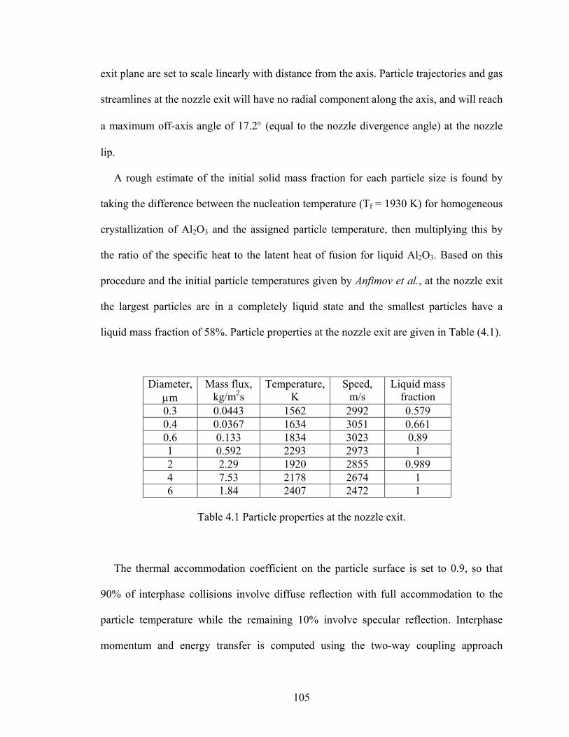
exit plane are set to scale linearly with distance from the axis. Particle trajectories and gas
streamlines at the nozzle exit will have no radial component along the axis, and will reach
a maximum off-axis angle of 17.2° (equal to the nozzle divergence angle) at the nozzle
lip.
A rough estimate of the initial solid mass fraction for each particle size is found by
taking the difference between the nucleation temperature (Tf = 1930 K) for homogeneous
crystallization of Al2O3 and the assigned particle temperature, then multiplying this by
the ratio of the specific heat to the latent heat of fusion for liquid Al2O3. Based on this
procedure and the initial particle temperatures given by Anfimov et al., at the nozzle exit
the largest particles are in a completely liquid state and the smallest particles have a
liquid mass fraction of 58%. Particle properties at the nozzle exit are given in Table (4.1).
Diameter, µm
Mass flux, kg/m2s
Temperature, K
Speed, m/s
Liquid mass fraction
0.3 0.0443 1562 2992 0.579 0.4 0.0367 1634 3051 0.661 0.6 0.133 1834 3023 0.89 1 0.592 2293 2973 1 2 2.29 1920 2855 0.989 4 7.53 2178 2674 1 6 1.84 2407 2472 1
Table 4.1 Particle properties at the nozzle exit.
The thermal accommodation coefficient on the particle surface is set to 0.9, so that
90% of interphase collisions involve diffuse reflection with full accommodation to the
particle temperature while the remaining 10% involve specular reflection. Interphase
momentum and energy transfer is computed using the two-way coupling approach
105

described in Chapters 2 and 3, and the crystallization of liquid Al2O3 droplets is
considered using the phase change model outlined in Section 4.3.
An axisymmetric simulation is performed on an unstructured rectangular grid
extending from the nozzle exit plane 100 m downstream and 40 m outward from the
central axis. The simulation is repeated for several different coupling parameter cutoff
values, where values for both gas-to-particle and particle-to-gas coupling are equal and
range from 0 to 0.1. Each case requires about 200 CPU hours on four 1.4 GHz AMD
Opteron processors.
4.4.2 Variation in calculated flow properties with cutoff values
Figure (4.1) shows the variation in the maximum downstream distance for interphase
coupling in either direction as a function of the cutoff values. Except for the largest cutoff
values considered, the length of the coupling domain is found to vary as roughly the
inverse square-root of the corresponding cutoff value. It follows that, as expected, smaller
cutoff values result in greater residence time for either particles or gas molecules within
the region where they may be influenced by interphase momentum or energy transfer.
In Fig. (4.2), the axial velocity component for the smallest particle size is plotted as a
function of the cutoff value for gas-to-particle coupling, at two different points located
50 m downstream from the nozzle exit plane and distances of 3.5 m and 14 m from the
central axis. Corresponding plots are given as Figs. (4.3) and (4.4) for particles of
intermediate size (1 µm diameter) and for the largest particles, respectively. As shown on
all three plots, farfield particle velocity varies significantly with the cutoff value C1 for
C1 > 10-4, while a relatively weak dependence is found for C1 ≤ 10-4.
106

Figure 4.1. Maximum downstream distance for interphase coupling.
Figure 4.2. Axial velocity component for 0.3 µm diameter particles as a function of cutoff
value C1 for gas-to-particle coupling.
107

Figure 4.3. Axial velocity component for 1 µm particles as a function of cutoff value.
Figure 4.4. Axial velocity component for 6 µm particles as a function of cutoff value.
108

Figure 4.5. Temperature of 0.3 µm particles as a function of cutoff value.
Figure 4.6. Temperature of 1 µm particles as a function of cutoff value.
109

Figure 4.7. Temperature of 6 µm particles as a function of cutoff value.
Figure 4.8. Variation in liquid mass fraction for 1 µm particles.
110

A similar trend is observed in Figs. (4.5) through (4.7), which show the variation with
C1 in particle temperature for the same three particle sizes and at the same two locations.
Again particle temperature is generally found to be a strong function of the cutoff value
only for C1 > 10-4. The one exception to this trend is found in Fig. (4.6), for 1 µm
diameter particles at the point (50,3.5). In this case, the average particle temperature
initially decreases as C1 is reduced from the maximum value of 0.1, due to the
corresponding increase in particle residence time within the gas-to-particle coupling
region where heat is transferred from particles to the colder surrounding gas. However,
for C1 < 10-3 the average particle temperature increases as C1 is further reduced. This is
explained by the fact that for this particular case, the residence time of 1 µm particles
within the gas-to-particle coupling region is great enough for a fraction of the initially
liquid particles to cool below the homogeneous crystallization temperature Tf = 1930 K.
Once the temperature of a liquid particle reaches Tf, the solidification process
immediately begins and the particle temperature increases following the energy balance
of Eq. (4.15). The fraction of 1 µm particles for which this process takes place will
increase for smaller values of C1, so the average temperature of these particles will
increase as a result.
This trend is further illustrated by Fig. (4.8), which shows the variation in liquid mass
fraction with C1 for the same particle size and location. For C1 > 10-3 all 1 µm particles at
this point are found to be entirely liquid, while the liquid mass fraction decreases for
smaller C1 to a value of 0.728 at C1 = 0. In both Figs. (4.6) and (4.8) the data point for
C1 = 0 is represented by a horizontal line through the vertical axis. Note that all other data
sets in Figs. (4.5) to (4.7) show monotonic trends through the full C1 range, as the phase
111

composition for these cases does not vary as a function of C1. At both locations and for
the full range of C1 values considered here, all 0.3 µm particles have completely
solidified, and all 6 µm particles are entirely liquid. In addition, 1 µm particles are
entirely liquid at the point (50,14) due to the reduced interphase heat transfer which
results from the relatively low gas number density far from the axis.
Various gas properties were examined at the same two flowfield locations, to
determine any dependence on the cutoff value C2 for particle-to-gas coupling. Of the
properties considered, only a weak dependence could be found for the gas translational
temperature, while the variation in all other properties was within statistical scatter. The
lack of C2 dependence can be attributed to the very small domains for particle-to-gas
coupling, as well as the dominance of the expansion process over interaction with the
particle phase in determining bulk gas properties far from the nozzle.
4.4.3 Relation between cutoff values and simulation efficiency
Figure (4.9) shows the variation with cutoff values (C1 = C2) in overall simulation
efficiency. The vertical axis here gives the total cpu time per time step at steady state,
normalized by the corresponding value when both cutoff values are set to zero. As
expected, simulation time is shown to decrease monotonically as cutoff values are
increased. For a given level of precision in simulation results, the use of coupling
parameters allows for a roughly 20% reduction in calculation time when cutoff values are
set to 10-6, or a 65% reduction when these values are set to 0.1.
Based on a comparison of Fig. (4.9) with the results discussed above, a cutoff value of
10-4 is recommended for both C1 and C2 in order to balance overall numerical efficiency
112

and accuracy in computed flow characteristics for both the particles and gas. As shown in
Fig. (4.9), the utilization of coupling parameters to identifying regions of negligible
interphase coupling results in a 30% reduction in simulation time when this cutoff value
is used. While no universal cutoff value can be found to optimize this balance under all
flow conditions, particularly when particle phase change is important, a value of 10-4 can
in general be expected to provide both reasonably good accuracy and efficiency.
Note however that the increase in efficiency associated with the use of these coupling
parameters does correspond to an unavoidable reduction in overall accuracy. While a
roughly 30% savings may not be considered sufficiently large to warrant implementation
of the method described here, the efficiency increase may under certain conditions be
much greater, particularly when the grid is extended to include the full domain of interest
for plume radiation signature analysis.
Figure 4.9. Total cpu time per time step at steady state, normalized by CPU time for the
zero cutoff values case.
113

4.4.4 Additional results
Selected results for the case where C1 = C2 = 10-4 are displayed in Figs. (4.10) and
(4.11). Figure (4.10) shows the contours of mass-averaged particle temperature and gas
translational temperature. As expected, particle temperatures are uniformly higher than
that of the surrounding gas, with the lowest particle temperatures occurring far from the
central axis where the smaller particles are concentrated. A slight reduction in average
particle temperature is found close to the axis, as a result of the increased heat transfer
toward the center of the plume nearfield region where the gas number density is greatest.
Contours of the Sauter mean particle diameter are shown in Fig. (4.11), along with the
overall liquid mass fraction for the particles. (The Sauter mean diameter is the diameter
of a particle with a volume-to-surface area ratio equal to that of the particle phase as a
whole, and is calculated as the ratio of mean-cubed to mean-squared particle diameters in
each cell.) The concentration of larger particles toward the axis is found to result in a
greater content of liquid alumina within this region, as the reduced surface area-to-
volume ratio among larger particles allows for a more gradual process of cooling and
solidification. Note that no streamwise variation is visible among any particle properties
shown in Figs. (4.10) or (4.11), due to the large difference in scale between the
simulation domain and the regions of significant interphase momentum and energy
exchange.
114

Figure 4.10. Contours of mass-averaged particle temperature (top) and gas translational
temperature. All values are in SI units.
Figure 4.11. Sauter mean particle diameter (top) and liquid mass fraction of particles.
115

Chapter V
An Alternate Approach for Gas Simulation
in Near-Equilibrium Regions
5.1 Overview and motivation
In this chapter a particle method is presented for the numerical simulation of rarefied
gas flows, based on the ellipsoidal statistical Bhatnagar-Gross-Krook (ES-BGK) model
of the Boltzmann equation. [Holway (1966)] The simulation procedure includes
consideration of rotational nonequilibrium, and enforces exact momentum and energy
conservation for a mixture involving monatomic and diatomic species. This method is
applied to the simulation of a rarefied nozzle expansion flow, and flowfield
characteristics are compared with experimental data as well as results from DSMC and
Navier-Stokes simulations of the same flow.
The ES-BGK method is shown from this comparison to allow for a relatively high
degree of accuracy in transitional flow regimes, while avoiding the intermolecular
collision calculations which typically make the DSMC simulation of low Knudsen
number flows prohibitively expensive. The procedures described here are intended for
implementation in a hybrid scheme along with traditional DSMC, to be used only in high
116
density flowfield regions where DSMC is particularly inefficient. Results from a series of
SRM plume simulations using this hybrid scheme are presented in Chapter 7.
5.1.1 Problems inherent in the DSMC simulation of SRM plume flows
As described in Chapter 1, the gas phase in a high altitude SRM exhaust plume
typically experiences a high degree of thermal nonequilibrium through much of the
flowfield. During the rapid expansion process just beyond the nozzle exit, the gas
velocity distribution begins to diverge significantly from the equilibrium limit, and
thermal energy is increasingly distributed non-uniformly among the translational and
internal degrees of freedom. Further downstream, these nonequilibrium effects continue
to increase as the gas rapidly expands and thermal energy is converted into energy
associated with bulk motion of the exhaust flow. Geometric effects lead to an imbalance
in the distribution of translational energy, where the translational temperature tends to be
higher in the streamwise direction than along transverse directions. [Boyd (2003)]
Rotational freezing occurs due to the combination of large gradients and low collision
frequency, and the flow ultimately approaches a near-free molecular regime where the
influence of collisional processes becomes negligible.
In engineering practice, the simulation of such highly rarefied flows is most often
performed using the DSMC method as discussed in Chapter 1. The DSMC method has
been shown to provide accurate solutions for highly rarefied nozzle and plume flows (see
for example Boyd et al. (1992)) and retains validity through the full range of possible
Knudsen numbers for a dilute gas. In theory then, DSMC may be applied to the entire
flowfield for a high altitude SRM exhaust plume.
117

The main obstacle, however, to DSMC calculations for this type of flow is the
enormous computational cost of simulating the higher density gas through much of the
plume nearfield region. There are three major factors which tend to make DSMC
prohibitively expensive, even on large parallel machines, for the simulation of relatively
high-density flows: First, for accurate simulation the cell size should ideally be much
smaller than any characteristic length scale for gradients in macroscopic flow quantities,
and nonphysical diffusion effects become increasingly significant as the cell size
increases. [Bird (1994), Breuer et al. (1995)] This generally limits cell dimensions to
roughly one mean free path, so that a very large number of cells may be required for the
simulation of even small-scale flows when the gas density is high. Second, the temporal
decoupling of collision and advection processes is in general a valid approximation only
if the time step is no larger than the local mean collision time. This means that for a high
density or low Knudsen number flow, a very large number of time steps may be required
to reach steady state conditions.
The above two requirements may be relaxed somewhat when macroscopic gradient
length scales are very large compared to the mean free path, so that the flow approaches a
near-homogeneous state. However, a third limiting factor for high density flows cannot
be relaxed under near-homogeneous conditions: The collisional process driving a flow
toward equilibrium is modeled in DSMC through the probabilistic calculation of
individual collisions between pairs of representative particles. (By convention, the term
“particle” is used throughout this chapter to designate a computational gas molecule
which represents a large number of actual molecules or atoms.) The collision frequency
increases with the gas density, so that for a fixed set of simulation parameters, a higher
118

density flow corresponds to an increase in the average number of collisions experienced
per particle during each time step. Under conditions typical in the plume nearfield region
of a high altitude SRM exhaust plume, this last requirement can make DSMC simulation
of such flows prohibitively expensive on all but the largest parallel machines.
5.1.2 The NS-DSMC hybrid approach
In practice, these plume flow simulations may be performed using a finite volume
representation of the Navier-Stokes (NS) equations in the high density regions where the
continuum and quasi-equilibrium assumptions underlying these equations are considered
valid. The DSMC method is then used only in the lower density regions where these
assumptions break down, and where a DSMC flowfield calculation is feasible using
available computational resources. The interface between NS and DSMC regions is
modeled either through an uncoupled matching of boundary conditions for two
independent simulations, or using a single hybrid code where the interface location may
be varied dynamically during the simulation through the evaluation of one or more
continuum breakdown parameters.
For either approach, the accurate determination of the boundary beyond which the NS
solution is invalid may be difficult and expensive. As a result, there is generally some
significant tradeoff between overall simulation accuracy and efficiency. Increased
accuracy results from a more precise or conservative determination of the proper
boundary for the NS domain. This in turn requires a greater computational load, either
through an iterative procedure to evaluate the boundary then update the overall flowfield
119

solution, or through an extension of the DSMC domain into regions which may be
accurately handled by the NS solver.
5.1.3 An all-particle hybrid scheme
This tradeoff between accuracy and efficiency may to some extent be avoided if an
alternate simulation approach is used in flowfield regions where the validity of the NS
equations is questionable, but the application of DSMC is particularly expensive. This
alternate method should be more efficient than DSMC in modeling relatively high density
flows, able to account for nonequilibrium phenomena which characterize a transition
Knudsen number regime out of range of NS solutions, and in good quantitative
agreement with both NS and DSMC for near-equilibrium flows. One such method is
presented here, using a particle-based probabilistic solution to the ellipsoidal statistical
Bhatnagar-Gross-Krook (ES-BGK) model of the Boltzmann equation.
In recent years, several authors have developed particle methods in which standard
DSMC collision operations are replaced by alternate procedures that account for the
collisional drive toward equilibrium, while avoiding the calculation of individual
collisions. [Montanero et al. (1998), Gallis and Torczynski (2000), Macrossan (2001),
Bruno, Longo, and Capitelli (2002), Bruno and Longo (2002)] In place of collision
calculations on pairs of representative particles, some fraction of particles is randomly
selected during each time step, and these particles are assigned new velocities according
to predetermined distribution functions.
In several of these methods, the collision process in each cell within the
computational grid is based on the homogeneous form of the Bhatnagar-Gross-Krook
120

(BGK) equation. [Bhatnagar, Gross, and Krook (1954)]
g g e(n ) / n ( )d f dt f f= −ν (5.1)
Here f is the velocity distribution function for a simple monatomic gas, fe is a Maxwellian
distribution with the same average and variance as f, ng is the number density, and ν is a
characteristic relaxation rate. This is a simplified linear model of the highly nonlinear
Boltzmann equation, valid under spatially homogeneous conditions. (See Chapter 1 for a
discussion of the Boltzmann equation, given as Eq. (1.1).) The detailed physics of the
collision term in the Boltzmann equation is ignored here in favor of a Maxwell-type
molecular model in which the entire distribution function f decays toward equilibrium at
a velocity-independent rate.
As proposed by Macrossan (2001) and independently implemented by Gallis and
Torczynski (2000) and Andries et al. (2000), the method may be modified for better
quantitative agreement with the Boltzmann equation as a solution to
g g G(n ) / n ( )d f dt f f= −ν (5.2)
where fG is an anisotropic Gaussian distribution function. This modification to the BGK
equation was proposed by Holway (1966) to correct for the nonphysical constraint in the
BGK model of unity Prandtl number, and has recently been shown to satisfy Boltzmann’s
H-theorem for entropy production. [Andries and Perthame (2001)] Following Cercignani
(1988), this is referred to here as the ellipsoidal statistical BGK (ES-BGK) model.
In addition to potential advantages in efficiency and accuracy over a NS/DSMC
hybrid scheme, an important advantage should be noted for the simulation of SRM plume
flows using a hybrid scheme involving DSMC and a particle method based on Eq. (5.2).
As described in previous chapters, the accurate simulation of these plume flows requires
121

implementation of a variety of models for the inclusion of solid and liquid particles,
including capabilities for strong two-way coupling between gas and condensed phase
properties. The hybrid NS/DSMC simulation of such multiphase flows may require a
large number of physical models to be independently implemented in the continuum NS
solver, in a manner which is consistent and easily integrated with corresponding models
in the DSMC code. By contrast, in an ES-BGK/DSMC hybrid scheme, only collision
calculations on gas phase particles are altered in high density regions, and all other
calculation procedures are left unchanged through the entire computational domain. As
no additional physical models are required in regions of near-equilibrium flow, ES-BGK
particle methods offer a significant advantage over NS solvers in ease of implementation
for the hybrid simulation of high altitude SRM plume flows.
In the remainder of this chapter, particle methods of Macrossan (2001) and Gallis
and Torczynski (2000) based on Eqs. (5.1) and (5.2) are extended for consideration of a
gas mixture involving monatomic and diatomic species, and a procedure is described to
enforce exact momentum and energy conservation in a flow involving rotational
nonequilibrium. A simple homogeneous test case is then used to verify the accuracy of
the proposed rotational relaxation model. Next, the method is applied to a nozzle flow
test case involving a small cold-gas thruster with N2 propellant exhausting into a vacuum,
and results are compared with DSMC, NS, and experimental data for the same flowfield.
Relatively good agreement is found between ES-BGK, DSMC and experimental results,
particularly in higher density regions near the nozzle throat. It is also shown that the ES-
BGK flowfield solution incorporates some nonequilibrium effects which are captured as
well by DSMC but neglected in the NS calculation.
122

5.2 Numerical procedure
As discussed in the previous section, all procedures unrelated to intermolecular
collisions in the ES-BGK particle method are identical to those in DSMC. However, the
process of calculating individual representative collisions is replaced by a procedure
which involves the resampling of particle properties from predetermined distributions.
All steps in these resampling calculations are described in this section, with a particular
emphasis on operations related to rotational nonequilibrium effects. The ES-BGK method
presented here is the first to allow for consideration of translational-rotational energy
exchange while enforcing exact conservation of momentum and energy.
5.2.1 Reassignment of particle velocities
Consider the ES-BGK collision procedure in a cell containing Ng particles, where
each particle may be assigned to one of several different monatomic or diatomic gas
species. We assume vibrational and electronic energy modes are unexcited, and the
variable hard sphere (VHS) collision model [Bird (1994)] is used to approximate the
variation of dynamic viscosity µ with translational temperature Tt. As a first step in the
method, Tt is calculated as a function of the average momentum and translational energy
of all particles in the cell:
(g 22t
B g
N1T m m3k (N 1) aaa= −
−u u )/ m (5.3)
Here m and u are the mass and velocity respectively of an individual particle, kB is
Boltzmann’s constant, the operator a designates an average over all particles in the
123

cell, and the notation x2 for any vector x is used to represent x⋅x. The coefficient
Ng/(Ng–1) in Eq. (5.3) corrects for a statistical error which appears when the traditional
formula for Tt based on the velocity distribution is applied to a discrete set of particle
velocities. [Sun and Boyd (2005)]
Using a first order Chapman-Enskog expansion of the ES-BGK equation, it can be
shown that the correct relations for heat flux and shear stress are recovered in a near-
equilibrium flow if the relaxation rate is given by
Pr pνµ
= ⋅ (5.4)
where Pr is the Prandtl number and p is the pressure. [Mieussens and Struchtrup (2004)]
From the ideal gas equation of state and the VHS approximation that µ scales with
temperature to some constant power ω, Eq. (5.4) may be rewritten as
ref 1g B t
ref
TPr n k Tω
ωνµ
−⎛ ⎞⎟⎜= ⋅ ⎟⎜ ⎟⎜⎝ ⎠ (5.5)
where Tref is a reference temperature and µref is the dynamic viscosity at Tref. For a simple
VHS gas, this viscosity can be calculated as a function of ω and the molecular collision
diameter dref at the reference temperature:
( )
( )( )
1/2B ref
ref 2ref
30 mk T /4 5 2 7 2 d
πµω ω
=− − (5.6)
Note that in most cases the value of dref is itself determined from experimental
measurements of µref. Eq. (5.6) is useful however in a hybrid code (discussed in Section
5.1) involving both DSMC and the method proposed here, as reference collision
diameters are among the required input parameters for DSMC collision calculations. A
simple approximate extension of Eq. (5.6) to a gas mixture may be obtained by summing
124
the product of µref and the time-averaged species mass fraction in the cell over all gas
species.
Once a relaxation rate ν has been determined, Eq. (5.2) may be integrated to give the
distribution function f after some finite time step ∆t as a linear combination of the initial
distribution f(0) and a corresponding anisotropic Gaussian distribution fG.
(5.7) (G( t) (0)exp( t) + 1 exp( t)f f fν∆ = − ∆ − − ∆ )ν
)
From Eq. (5.7), we determine the number of particles Nv selected for reassignment of
velocity components as
([ ]floorv gN N 1 exp( t) Rν= − − ∆ + (5.8)
where ν is evaluated using Eq. (5.5), R is a random number in [0,1] and the operator
“floor” rounds to the nearest smaller integer. Note that a time-averaged value of the
number density ng should be used in Eq. (5.5) to avoid an error associated with statistical
fluxuations in the calculated relaxation rate. Once Nv is known, this number of unique
particles is then randomly selected and assigned to a list for velocity resampling. (In
order to reduce calls to the random number generator, if Nv>½Ng then Ng–Nv randomly
chosen particles are removed from a list which initially includes all particles in the cell,
and the remaining particles are used for resampling.) In the special case where Nv = 1,
momentum conservation requires that the velocity of the selected particle remains
constant, so that Nv values of zero and one are equivalent during the resampling
procedure. To correct for the resulting error, if Nv is calculated as one through Eq. (5.8)
then an additional random number is generated and Nv is set with equal probability to
either zero or two.
After Nv particles have been selected, all velocity components of these particles are
125
resampled from a normalized Maxwellian distribution. Each velocity component is set to
either
*i 1 2u cos(2 ) ln( )/R Rπ= − m or *
i 1 2u sin(2 ) ln( )/R Rπ= − m
u
(5.9)
where the subscript i denotes the direction, m is the particle mass, and R1 and R2 are
random numbers between 0 and 1. Two statistically independent values of ui* may be
obtained if Eqs. (5.9) are evaluated for the same values of R1 and R2, so that only a single
random number must be generated per velocity component. Following Gallis and
Torczynski (2000), all resampled velocities are then modified to give new values ci(1)
which conform to an anisotropic Gaussian distribution:
(5.10) (1) *ij jiu S=
where
( )gij ij i j i j ij
B t g
N1 Pr 1S mu u mu mu / m2Pr k T N 1 aaa aδ δ
⎡ ⎤− ⎢ ⎥= − −⎢ ⎥−⎣ ⎦−
eq
(5.11)
Here δij is the Kronecker delta, ui and uj are particle velocity components before
resampling, Tt is evaluated using Eq. (5.3), and the superscript (1) indicates a newly
reassigned value.
5.2.2 Rotational energy resampling
To account for the effect of collisions on the rotational energy distribution among
diatomic gas species, we define a rotational relaxation rate νr such that, in a
homogeneous gas, the instantaneous cell-averaged rotational temperature Tr will vary as
r r rT / (T T )d dt ν= − − (5.12)
Here Teq is the equilibrium temperature to which both Tr and Tt converge after a long
126

period of time, and Tr is given by
r r aaB
2T /kE ζ= r (5.13)
The above symbols Er and ζr denote rotational energy and rotational degrees of freedom,
respectively, for an individual particle. Substitution of Eq. (5.13) into Eq. (5.12) gives the
familiar equation of Jeans (1916) for the relaxation of internal energy modes.
The equilibrium temperature Teq can be expressed as a weighted sum of the rotational
and translational temperatures
( )t,eff t r r t,eff r eqaT Tζ ζ ζ ζ+ = + a T (5.14)
where ζt,eff is the effective number of translational degrees of freedom for all particles in
the cell. If all Ng particles are together considered as an isolated system, then it follows
from Eqs. (5.3) and (5.13) and energy conservation arguments that
0g2 aa B t r B rag
N -1m / m 3 k T k T
Nddt
ζ⎡ ⎛ ⎞⎟⎜⎢ ⎥+ +⎟⎜ ⎟⎟⎜⎜⎢ ⎥⎝ ⎠⎣ ⎦u
⎤= (5.15)
while momentum and mass conservation require that the first term within the brackets be
constant in time as well. By comparing Eqs. (5.14) and (5.15) and noting that Teq is a
time invariant quantity, it can be shown that there are effectively 3(Ng-1)/Ng translational
degrees of freedom in the cell, so that the equilibrium temperature may be given from Eq.
(5.14) as
( )( )( )g g t r a
eqg g r a
3 N -1 /N T TT
3 N -1 /Nζζ
+=
+r
(5.16)
Note that the arguments used to derive Eq. (5.16) make no assumptions regarding
how the translational and rotational temperatures relax toward the equilibrium state, so
that this equation should also be valid for DSMC and other methods for which a discrete
127

set of particle velocities is used to describe the velocity distribution of a gas in rotational
nonequilibrium. As there are exactly three translational degrees of freedom for any real
gas under consideration here, this derivation reveals the existence of a deterministic error
which scales as (Ng-1)/Ng and may significantly influence calculated bulk flow properties
when the average number of particles per cell is very small. While it appears that no
previous references to this error source exist in the literature, the upper bound of the
resulting error should be relatively small (less than 5%) when particle numerical weights
are set such that over 20 particles are assigned to each cell, as is standard practice in
DSMC.
The rotational relaxation rate νr shown in Eq. (5.12) is defined here as the frequency
of inelastic collisions, given as the ratio of the collision frequency Fcoll to the rotational
collision number Zr. To determine Fcoll, consider a cell containing particles of Nspec
different species, each with a mass mi, VHS reference collision diameter dref,i and number
density ni averaged over a large number of time steps. Assuming a near-equilibrium flow,
we can efficiently calculate the collision frequency as
coll
specN i1B ref t
i j ij ijg ref i 1 j 1
4 k T Tn n A (2 )
n 2 TF
ωδ
π
−
= =
⎛ ⎞⎟⎜= −⎟⎜ ⎟⎜⎝ ⎠ ∑ ∑ (5.17)
where
( )2 i jij ref,i ref,j
i j
m mA d +d
4 mπ +
=m
and ng is the sum of ni values over all Nspec species. Note that no implied summations are
used in the index notation of Eq. (5.17).
The rotational collision number Zr is calculated using a modified form of a formula
given by Parker (1959).
128

rr 1/2 * 1/2 2 *
eq eq
3/5 ZZ
1 ( /2)(T /T ) ( / 4)(T /T )π π π
∞=+ + + (5.18)
The above constants Zr∞ and T* are determined for N2 as Zr
∞=23.0 and T*=91.5 K. [Bird
(1994)] As a modification to Parker’s formula, the equilibrium temperature Teq is used
here in place of Tt following observations of Boyd (1990) that, for a single intermolecular
collision, Zr tends to vary as a function of both the translational and rotational collision
energies. The 3/5 factor in the numerator, also not in Parker’s original formula, accounts
for the fact that Zr is defined here to characterize the rate at which Tr relaxes toward Teq,
not toward Tt as used by Parker and others. [Bird (1994)]
By analogy with Eq. (5.8), Eq. (5.12) can be integrated in time to give an initial
estimate of the number of particles Nr for which to resample rotational energy as
collr g
rN N 1 exp t
ZF⎛ ⎛ ⎟⎟⎜ ⎜≈ − − ∆ ⎟⎟⎜ ⎜ ⎟⎟⎜ ⎜⎝ ⎝
⎞⎞⎠⎠
R
(5.19)
where Fcoll and Zr are evaluated using Eqs. (5.17) and (5.18) respectively. (The exact
determination of Nr requires a more involved procedure, and is discussed in detail
below.) In the implementation proposed here, Nr particles are randomly selected from the
list of Nv particles which have already been tagged for velocity resampling, and the
rotational energy Er of each selected diatomic particle is reassigned to a normalized value
(5.20) (1)r ln( )E = −
where a unique random number R∈(0,1] is used for each particle.
5.2.3 Momentum and energy conservation
To avoid random walk errors and permit overall accuracy for a near-equilibrium flow
comparable to that of either DSMC or NS simulations, we desire for both momentum and
129
energy to be exactly conserved during the resampling procedures. It follows that all
reassigned velocities u(1) and rotational energies Er(1) must be modified to final values u(2)
and Er(2) such that
(2) (0)v
m m=u uv (5.21)
and
(2) 2 (2) (0) 2 (0)v r r v rv r v
1 1N m( ) N N m( ) N2 2
E E+ = +u u r r (5.22)
where the operators v and r denote averages over all particles used in the
resampling of velocity and rotational energy respectively. Further, to satisfy energy
equipartition at the equilibrium limit, translational and rotational temperatures based on
reassigned values must be equal. This condition can be written as
( )2v (2) 2 (2) (2)v r rv v rB v B
1 N 2m( ) m / m /
3k (N 1) kE ζ− =
−u u r (5.23)
where ζr is the number of rotational degrees of freedom for an individual particle. For
each of the Nv particles selected for velocity resampling, the final velocity is calculated as
((2) (1) (1)vv
m / mC= + −u u uB )
r
(5.24)
while each of the Nr particles with resampled rotational energies is given a final value of
. (5.25) (2) (1)rE DE=
By algebraic manipulation of Eqs. (5.21) through (5.25), it can be shown that momentum
conservation, energy conservation and energy equipartition are all satisfied if the vector
B and scalar constants C and D are chosen as follows:
(0)vv
m / m= uB (5.26)
130
( )( )
( )1/22(0) 2 (0) (0)
v r v rv v v r2(1) 2 (1)v r r r vv v
m( ) m / m 2 N /N3 N 13 N 1 N m( ) m / m
EC
ζ
⎡ ⎛ − + ⎟⎜⎛ ⎞−⎢ ⎥⎟⎜⎟⎜ ⎟= ⎜⎟⎢ ⎥⎜ ⎟⎟⎜⎟⎜ ⎟− +⎝ ⎠⎢ ⎥⎜ ⎟− ⎟⎜⎝ ⎠⎢ ⎥⎣ ⎦
u u
u u
⎞⎤ (5.27)
( )
( )2(0) 2 (0) (0)v r v rv r v v
(1)v r r r r r
m( ) m / m 2 N /NN3 N 1 N 2
ED
Eζ
ζ
⎛ ⎞− + ⎟⎜⎛ ⎞ ⎟⎜⎟⎜ ⎟= ⎜⎟⎜ ⎟⎟⎜⎟⎜ ⎟− +⎝ ⎠⎜ ⎟⎟⎜⎝ ⎠
u ur (5.28)
5.2.4 A correction factor for the rotational relaxation rate
From the definition of rotational temperature indicated by Eq. (5.13), the right hand
side of Eq. (5.28) may be expressed as a ratio of temperatures: The denominator gives the
rotational temperature based on values of Er(1), while the numerator gives the temperature
corresponding to the conditions of Eq. (5.23). Thus, Eq. (5.28) may be used to show that
the temperature T(2) based on resampled and renormalized values of either particle
velocity u(2) or rotational energy Er(2) can be given as
( )2v B r(2) (0) 2 (0) (0)
v rv vv r r vr
N /k NT m( ) m / m3 N 1 N N
Eζ
⎛ ⎞⎛ ⎛⎟⎜ ⎟⎜ ⎜= − +⎟ ⎟⎜ ⎜ ⎜ ⎟⎜ ⎜⎟⎟⎜ ⎝ ⎝− +⎝ ⎠u u
r2 ⎞ ⎞⎟⎟⎟⎠ ⎠ . (5.29)
As particles are randomly chosen for velocity or rotational energy resampling, the
averaged quantities in Eq. (5.29) will, on average, equal the corresponding quantities
averaged over all N particles in the cell. If we denote the equivalent temperature based on
cell-averaged values as Ta(2), then it follows from substitution of Eqs. (5.3) and (5.13)
into Eq. (5.29) that
( )( )( )v r t r(2) a
av r r a
3 N -1 /N T TT
3 N -1 /Nζζ
+=
+r . (5.30)
As the temperature Ta(2) is generally not equal to the equilibrium temperature Teq
determined from Eq. (5.16), the procedure used to calculate Nr must be based on a
relaxation rate other than the true characteristic rate for rotational relaxation νr = Fcoll/ Zr.
131

A correction factor β is therefore introduced as the ratio of this required relaxation rate to
νr, so that in a homogeneous adiabatic flow,
. (5.31) (2)r r rT / (T T )d dt βν= − − a
From a comparison of Eqs. (5.12) and (5.31), it follows that
(2)r eq r a(T T ) (T T )β = − − . (5.32)
Substituting Eqs. (5.16) and (5.30) into Eq. (5.32), we find
( )( )
β*
r r va
r g ga
3 N / N3 N / N
ζζ
+=
+-1-1 (5.33)
where Nr* is an approximation to the integer value Nr based on an exact solution to Eq.
(5.31). If Eq. (5.31) is integrated over the time step interval ∆t, then the same reasoning
used to find Nv by Eq. (5.8) may be used to calculate Nr* as
coll*r
rN = 1 exp ∆t
ZFβgN ⎛ ⎛ ⎟⎟⎜ ⎜− − ⎟⎟⎜ ⎜ ⎟⎟⎜ ⎜⎝ ⎝
⎞⎞⎠⎠ . (5.34)
Note from Eqs. (5.33) and (5.34) that β and Nr* cannot be independently determined,
but must instead be calculated simultaneously using an iterative method. In the
implementation proposed here, β is initially set to one and Nr* is found by Eq. (5.34),
after which β and Nr* are updated using Eqs. (5.33) and (5.34) respectively. This
procedure is repeated four additional times, after which the number of particles to select
for rotational energy resampling is computed as Nr = floor[Nr* +R] where R is a random
number in [0,1]. This simple “brute force” approach is found to give a reasonable balance
of accuracy and efficiency over a wide range of conditions, and more complicated
iterative schemes with faster convergence should not generally be required due to the
insignificant contribution of this procedure to the total computational expense.
132

5.3 Homogeneous rotational relaxation
To verify the accuracy of the scheme for rotational relaxation, all procedures
described in the previous section are implemented in a modified version of the DSMC
code MONACO [Dietrich and Boyd (1996)] and applied to a zero-dimensional test case
based on simulations of Bird (1994). An isolated control volume of N2 gas is given initial
conditions involving translational equilibrium at 500 K and a rotational temperature of
0 K. The simulation domain consists of a single cell with specularly reflecting walls and
10,000 particles, and the time step is set to 1/2 of the initial mean collision time. The
rotational collision number is found from Eqs. (5.16) and (5.18) to hold a constant value
of Zr = 4.31, so that the rotational and translational temperatures will vary in time
according to analytical expressions similar to those derived by Bird (1994).
r tcoll coll
t tT , T4.31τ τ
300 1 exp 300 200 exp4.31
⎛ ⎛ ⎞⎞ ⎛⎟⎟ ⎟⎜ ⎜ ⎜⎟⎟ ⎟⎜ ⎜ ⎜= − − = + −⎟⎟ ⎟⎜ ⎜ ⎜⎟⎟ ⎟⎟⎟ ⎟⎜ ⎜ ⎜⎜ ⎜ ⎜⎝ ⎝ ⎠⎠ ⎝
⎞
⎠
'
(5.35)
Here both temperatures Tt and Tr are given in K, t is the total elapsed time and τcoll is a
characteristic mean collision time. The variable τcoll may be defined in terms of the
instantaneous mean collision frequency Fcoll as
coll collt t' tτ-1t
0( )F d⎡ ⎤= ⎢ ⎥⎣ ⎦∫ (5.36)
where Fcoll is calculated for a VHS gas using Eq. (5.17).
133

Figure 5.1. Time variation in temperatures for rotational relaxation.
Figure (5.1) shows the variation in both Tr and Tt as functions of the normalized time
t/τcoll. Results from the ES-BGK simulation are presented along with results from a
DSMC simulation under identical conditions, and theoretical curves based on Eqs. (5.35)
are also shown for comparison. For consistency, a constant rotational collision number of
4.31 is used in the DSMC simulation. The ES-BGK data points are found to be in close
agreement with both theory and DSMC, while a slight underprediction is observed in the
relaxation rate from the ES-BGK simulation. This discrepancy can be traced to the fact
that only a fraction of particles are chosen for velocity resampling during each time step.
If the artificial condition Nv=Ng is imposed, then nearly perfect agreement is found
between the ES-BGK and theoretical curves of Fig. (5.1).
As discussed by Bird (1994), even DSMC results for homogeneous rotational
relaxation with constant Zr can only be approximated by an analytical solution, and the
134

scale of the disagreement between DSMC and theoretical curves is comparable to that
between theory and ES-BGK. Both DSMC and ES-BGK results have some dependence
on the VHS temperature exponent ω, so by comparison with DSMC we can conclude that
rotational relaxation is modeled with acceptable accuracy by the method proposed here.
5.4 Nozzle flow simulation
Relatively little published experimental data may be considered appropriate for
evaluation of the proposed ES-BGK method under conditions similar to those expected in
the SRM plume flows of interest. The most detailed set of flowfield property
measurements for a suitable rarefied expansion flow is likely that of Rothe (1971), where
an electron beam technique is used to measure density and rotational temperature for the
flow of N2 through a very small nozzle into a vacuum chamber.
Both NS and DSMC simulations of the internal nozzle flow have been performed by
Chung et al. (1995) In the DSMC simulation by these authors, the computational domain
is restricted to the lower density regions beyond the nozzle throat, with inflow conditions
at the throat based on a NS simulation of the flow within the convergent section of the
nozzle. Generally good agreement is found between DSMC results and experimental
data, while a NS simulation of the entire nozzle flow gives relatively poor agreement
with the experiment in areas downstream of the throat where nonequilibrium effects
become significant.
135

5.4.1 Simulation setup and boundary conditions
To evaluate the accuracy of the ES-BGK approach presented here, ES-BGK and
DSMC simulations are performed for the divergent nozzle and nearfield plume flow
investigated by Rothe (1971). Identical grids, boundary conditions and numerical weights
are used for the two simulations, with the same grid geometry and inflow conditions at
the nozzle throat employed in the DSMC simulation of Chung et al. (1995) As the ES-
BGK particle method is based on assumptions of near-equilibrium flow, we can
investigate the applicability of the method to higher Knudsen number regimes by
comparing ES-BGK results with both DSMC and experimental data.
Following Chung et al. we use a VHS temperature exponent (ω) of 0.24 and assume
fully diffuse reflection for particle collisions with the nozzle wall. These authors
investigated a number of different models for translational energy transfer during
particle-wall collisions, and found best agreement with experimental data when all
collisions are assumed diffuse, with a 10% probability of thermal accommodation to the
wall temperature of 300 K. Energy exchange between translational and rotational modes
was calculated using a detailed model which allows the exchange probability to vary as a
function of the total incident energy of the colliding particle.
As noted by Chung et al., a lack of experimental measurements on the interaction of
N2 gas with solid graphite (the nozzle wall material) leaves some doubt as to the validity
of this energy exchange model. A more commonly accepted procedure for modeling
rotational energy transfer during particle-wall collisions in DSMC involves an
assumption that particle rotational energy is resampled from an equilibrium distribution
at the wall temperature with some uniform probability. Therefore, as a simplification to
136

the procedure described by Chung et al., it is assumed here that 10% of particle-wall
collisions involve full accommodation of both translational and rotational energy to the
wall temperature, and the remaining 90% of these collisions involve adiabatic diffuse
reflection. In the latter type of collision, the post-collision direction of the particle
trajectory is randomly assigned according to the equilibrium velocity distribution for
particles which pass through a plane, while the incident values of both translational and
rotational energy are retained.
Figure 5.2. Grid geometry for ES-BGK and DSMC simulations.
Axisymmetric ES-BGK and DSMC simulations are performed on a 1.4 GHz AMD
Athlon cluster, with static domain decomposition among eight separate tasks. Each
calculation is run for 24 hours, with roughly 15 million particles at steady state and an
unstructured grid of about 41,000 triangular cells scaled according to the local mean free
path. The grid geometry is shown in Fig. (5.2) following that used by Chung et al. Not
visible in the figure is the wall curvature at the throat, where the radius of curvature is
one half the throat radius of 2.55 mm. The nozzle divergence angle is 20°, the exit-to-
throat area ratio is 66, and the simulation domain extends 14 mm downstream of the exit
137
plane. To avoid unphysical flow characteristics beyond the exit plane due to the small
domain size, we neglect the effect of ambient pressure in the vacuum chamber and use
outflow boundaries within the plume region.
5.4.2 Comparison of flowfield property contours
Mach number contours for both ES-BGK and DSMC simulations are shown in Fig.
(5.3), where the top half and bottom half of the figure give ES-BGK and DSMC results
respectively. Excellent agreement between the two methods is found in the area around
the nozzle throat. In both simulations, a significant reduction in Mach number is found
toward the centerline in this region, as results from a weak compression wave due to the
curvature of streamlines at the throat. [Chung et al. (1995)] Mach number contours along
the nozzle wall are also nearly identical, and both results show a termination of the sonic
line at the nozzle lip due to the rapid acceleration expected at the lip in any highly
underexpanded nozzle flow.
In contrast, prominent differences between the two results appear along the centerline
beyond a point about 1 cm downstream of the throat. As the degree of rarefaction
increases with downstream distance, the centerline Mach number gradient in the DSMC
simulation becomes significantly greater than in the ES-BGK simulation, so that the
intersection of the Mach 4 contour line with the axis occurs roughly 2.6 cm further
upstream in DSMC than in ES-BGK results. This difference in Mach number is likely a
result of the unphysical lack of velocity dependence in the collisional relaxation rate of
Eq. (5.2), which should correspond to some reduction in the streamwise temperature
gradient within areas of low collision frequency. The difference between the results is
138

however largely restricted to a narrow region along the axis, and very good agreement
between the two sets of contours is still found well downstream of the throat at points
further from the centerline. Note that no contour lines are shown within the plume
backflow region beyond the nozzle lip, due to the small sample size in this very low
density region.
Figure 5.3. Mach number contours for ES-BGK (top) and DSMC (bottom).
Contours of density are shown in Fig. (5.4), again with ES-BGK results in the top half
and DSMC results in the bottom half of the figure. All values are normalized by the
stagnation density ρo = 5.323×10⁻³ kg/m3. As in Fig. (5.3) we find excellent agreement
around the nozzle throat and further downstream in regions far from the centerline. Both
results show an off-axis local maximum in the density profile just downstream of the
throat, which is consistent with a weak compression wave described by Chung et al.
(1995) and mentioned above in the discussion of Mach number contours. As above, the
139
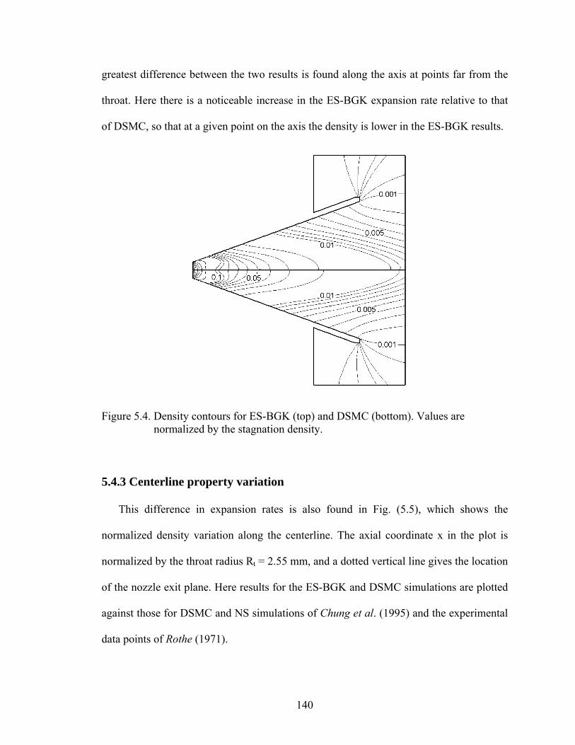
greatest difference between the two results is found along the axis at points far from the
throat. Here there is a noticeable increase in the ES-BGK expansion rate relative to that
of DSMC, so that at a given point on the axis the density is lower in the ES-BGK results.
Figure 5.4. Density contours for ES-BGK (top) and DSMC (bottom). Values are normalized by the stagnation density.
5.4.3 Centerline property variation
This difference in expansion rates is also found in Fig. (5.5), which shows the
normalized density variation along the centerline. The axial coordinate x in the plot is
normalized by the throat radius Rt = 2.55 mm, and a dotted vertical line gives the location
of the nozzle exit plane. Here results for the ES-BGK and DSMC simulations are plotted
against those for DSMC and NS simulations of Chung et al. (1995) and the experimental
data points of Rothe (1971).
140

Figure 5.5. Density variation along the nozzle centerline.
For x/Rt < 10 very similar centerline density profiles are found for the two
simulations presented here, and a slight difference is observed between these and the
DSMC and NS contours given by Chung et al. The reason for this discrepancy is not
clear, but two likely possibilities are some difference in grid resolution within this region
between the two sets of simulations, or a discretization of flow conditions at the nozzle
throat from the use of a finite number of uniform inflow boundaries. In general, the ES-
BGK result agrees very well with both DSMC density profiles and the experimental
values. A significantly higher level of overall accuracy is found in the ES-BGK results
than in those from the NS simulation, particularly far downstream of the throat where
density is slightly underpredicted by ES-BGK but greatly overpredicted by the NS
approach.
141

Figure 5.6. Variation of rotational and translational temperature along the centerline.
Figure (5.6) shows the variation in translational and rotational temperature along the
nozzle centerline for ES-BGK and both DSMC simulations, along with the NS centerline
temperature and rotational temperature values of Rothe (1971). All temperatures here are
normalized by the stagnation temperature To = 300 K. In comparing the two temperature
profiles from the ES-BGK simulation, note that the rotational temperature is uniformly
higher than the translational temperature, and that the difference between the two values
increases with downstream distance. This trend is also observed in both sets of DSMC
results, and demonstrates the rotational energy lag expected in rarefied expansion flows
due to a finite rotational relaxation time. The quantitative level of agreement between the
experimental measurements and ES-BGK results is in general comparable to that
between the experiment and DSMC, although the ES-BGK rotational temperature near
the nozzle exit is significantly higher than that found using the other methods.
142
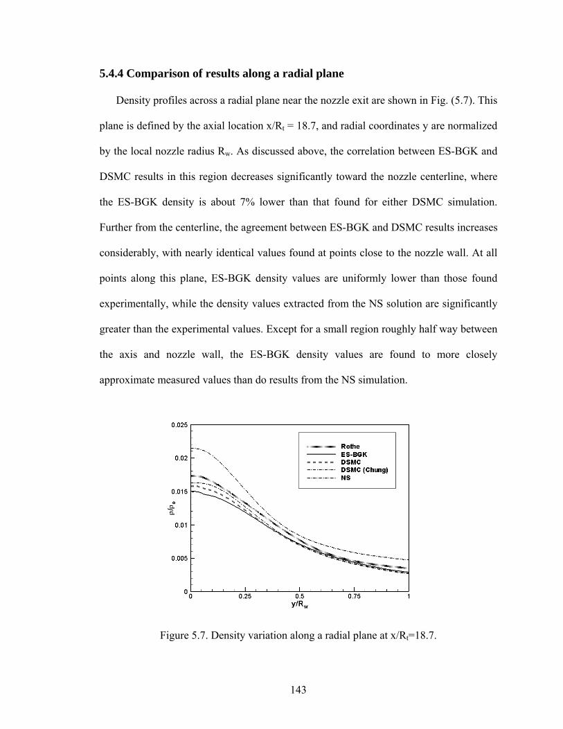
5.4.4 Comparison of results along a radial plane
Density profiles across a radial plane near the nozzle exit are shown in Fig. (5.7). This
plane is defined by the axial location x/Rt = 18.7, and radial coordinates y are normalized
by the local nozzle radius Rw. As discussed above, the correlation between ES-BGK and
DSMC results in this region decreases significantly toward the nozzle centerline, where
the ES-BGK density is about 7% lower than that found for either DSMC simulation.
Further from the centerline, the agreement between ES-BGK and DSMC results increases
considerably, with nearly identical values found at points close to the nozzle wall. At all
points along this plane, ES-BGK density values are uniformly lower than those found
experimentally, while the density values extracted from the NS solution are significantly
greater than the experimental values. Except for a small region roughly half way between
the axis and nozzle wall, the ES-BGK density values are found to more closely
approximate measured values than do results from the NS simulation.
Figure 5.7. Density variation along a radial plane at x/Rt=18.7.
143

Figure 5.8. Temperature variation along a radial plane at x/Rt=18.7.
Profiles of rotational and translational temperature along the same radial plane are
shown in Fig. (5.8). In comparing the ES-BGK rotational temperature profile with that
from the DSMC simulation performed here, we find an overestimate of about 13% in the
ES-BGK values near the axis, and a slight underestimate (less than 1%) at the nozzle
wall. The same general pattern is also observed in a comparison of translational
temperature profiles, although the translational temperature is underpredicted in the ES-
BGK simulation by roughly 3% at the wall. While some of these discrepancies are
significant, the general trends shown in the DSMC results are qualitatively reproduced
very well by the ES-BGK method: The rotational temperature is slightly higher than the
translational temperature for y/Rw < 0.7, with a sign reversal in the temperature difference
beyond this point. At the nozzle wall, the translational temperature is almost fully
144

accommodated to the wall temperature, while the rotational temperature is considerably
lower.
The difference between translational and rotational temperatures at the wall in both
the ES-BGK and DSMC results may be attributed to the wall collision model. All
particle-wall collisions are diffuse, so that the translational component of average thermal
energy for reflected particles corresponds to either the wall temperature or the local
stagnation temperature as measured by the velocity of incident particles. As the wall and
stagnation temperatures are nearly equal, we expect a very small difference between the
wall surface temperature and the gas translational temperature at the wall. In contrast, the
average post-collision rotational energy of particles involved in adiabatic diffuse
reflection corresponds to the rotational component of the gas static temperature, not the
stagnation temperature. Rotational energy accommodation occurs for only a small
fraction of wall collisions, so there should be relatively little difference in the average
rotational energy between incident and reflected particles.
In low density regions where the rotational relaxation time is large compared to other
characteristic time scales for the flow, a significant lag may develop between rotational
and translational temperatures. As the region under consideration has both a large
rotational relaxation time and a boundary condition which tends to disproportionately
increase the translational temperature, the trends observed at the wall in Fig. (5.8) seem
physically justified.
Note that the NS simulation does not account for rotational nonequilibrium, so only a
single temperature for this simulation is shown in the figure. The NS temperature profile
shows relatively poor agreement with all of the other results, and gives a gas temperature
145

at the wall between the translational and rotational temperatures found using the other
methods. A no-slip adiabatic boundary condition is used for the wall in the NS
calculation, so some temperature discontinuity at the wall is expected.
Figure 5.9. Axial velocity profiles at x/Rt=18.7.
Profiles of bulk axial velocity are shown in Fig. (5.9), again at the radial plane near
the nozzle exit defined by x/Rt = 18.7. Velocities here are normalized by the most
probable thermal speed at the stagnation temperature So = (2RTo)½ = 422 m/s. Nearly
identical profiles are found for the ES-BGK and the two DSMC simulations, with a
deviation between the three results of less than 5% at all points on the plot. The NS
velocity profile shows excellent agreement with the other results at the centerline, but
diverges significantly within a short distance from the axis. While the ES-BGK and
DSMC simulations give a wall slip velocity equal to about 28% of the centerline velocity,
the NS no-slip boundary condition results in a velocity of zero at the wall. If a Maxwell-
type slip model (based on the velocity gradient at the wall) had been employed in the NS
146
simulation, we expect that better agreement would be found between the NS velocity
profile and those for the other methods. A slip model would however affect density and
temperature profiles as well, so it is not clear that its inclusion would lead to a net gain in
overall accuracy for the NS simulation of this flow.
5.4.5 Evaluation of continuum breakdown
Figure (5.10) displays the variation along the centerline of continuum breakdown
parameters, based on the DSMC simulation performed for this study. As defined by
Boyd, Chen and Candler (1995), the local degree of thermal nonequilibrium may be
roughly characterized by the maximum value of a gradient length local Knudsen number
KnGLL(Q), where
GLLQKn (Q)
Q sλ ∂=
∂ (5.37)
and Q is set to either the density, translational temperature or bulk speed of the gas. The
symbol λ here denotes the mean free path, and ∂Q/∂s is the partial derivative of Q in the
direction of maximum gradient. As radial derivatives of macroscopic flow quantities are
by definition zero along the centerline, ∂s here is in the axial direction. Significant scatter
is observed among data points in the figure, as a result of both statistical noise and
subtractive cancellation error in the evaluation of the derivatives. Tenth order polynomial
trend lines, based on a least-squares fit, are therefore used to more clearly show the
general trends among the three different parameters.
147

Figure 5.10. Continuum breakdown parameters along the nozzle centerline.
As is generally expected for a near-adiabatic expansion flow, the parameter based on
density KnGLL(ρ) gives the largest value through nearly the entire range considered.
Based on this parameter, a local maximum in the degree of nonequilibrium is found a
short distance downstream of the throat. This maximum can be attributed to the large
curvature of streamlines around the throat, and the associated weak compression wave
mentioned in the discussion of Figs. (5.3) and (5.4). The flow then equilibrates somewhat
before rarefaction effects again become more prominent further downstream. A
maximum KnGLL(ρ) value of slightly less than 0.025 is ultimately reached in the nearfield
plume region just upstream of the outflow boundary. Trends in this parameter are found
to correlate well with the general level of agreement between ES-BGK and DSMC results
as shown in Figs. (5.3) through (5.6). As the value of KnGLL(ρ) increases with
downstream distance along the centerline, translational and rotational temperatures are
148
increasingly overpredicted by the ES-BGK method, while density and Mach number are
underpredicted.
5.4.6 Considerations of computational expense
It should be noted that the comparison of ES-BGK simulation results with DSMC, NS
and experimental data is intended to assess the validity of the assumptions and
approximations behind the method itself, and not to evaluate the tradeoff between
efficiency and accuracy at larger time steps where advantages of the ES-BGK method
over DSMC become apparent. However, if computational expense is measured as the
mean calculation time per particle per time step at steady state, the ES-BGK simulation
presented here is about 9% less expensive than the DSMC simulation. While this figure
may seem discouraging, the ES-BGK calculations are not performed under conditions for
which this method is intended in a practical engineering application, but instead under
conditions where traditional DSMC techniques are more appropriate due to the relatively
large Knudsen number regimes encountered here.
Throughout the computational domain, the time step used in both ES-BGK and
DSMC simulations is no greater than the local mean collision time, as is standard practice
in DSMC. (Through much of the flowfield, the time step is in fact several times smaller
than the mean collision time.) The use of such a small time step contributes to a high
degree of confidence in the overall accuracy of the DSMC simulation, and allows the ES-
BGK simulation to be performed under conditions where several assumptions behind this
method are known to be valid. In particular, the temporal decoupling of particle
advection and collision processes in both ES-BGK and DSMC is strictly valid only when
149

this decoupling occurs over time scales smaller than the mean collision time. The above
comparison should therefore be viewed as an evaluation of the ES-BGK method under
ideal conditions where the accuracy of this method in a rarefied expansion flow can be
properly assessed.
As discussed in Section 5.1, the proposed scheme is not intended as an alternative to
DSMC as a general simulation method for nonequilibrium gas flows, but instead is meant
for implementation in a hybrid code to simulate flows involving a wide range of Knudsen
number regimes. In the intended application of this code, standard DSMC techniques are
used in regions of highly nonequilibrium flow where DSMC is most appropriate, and ES-
BGK calculations are performed only in higher density transition regime and continuum
flow regions where DSMC may be prohibitively expensive. The boundary between
DSMC and ES-BGK domains is determined according to standard continuum breakdown
parameters such as Eq. (5.37). With the exception of areas close to this boundary, the ES-
BGK procedures will be applied primarily to regions where, for computational efficiency,
the time step and cell size are significantly larger than the mean collision time and mean
free path respectively.
As the time step and cell size increase, some additional loss of accuracy is expected in
the ES-BGK results, due to an error associated with the temporal and spatial decoupling
of collision and advection processes in the gas, as well as a nonphysical equilibration of
flow properties in each cell and an increase in numerical diffusion effects. [Breuer et al.
(1995)] At the same time, the computational expense of collision procedures will
approach an asymptotic limit where all particle velocity and rotational energy values are
reassigned during each time step. In contrast, DSMC collision procedures either give
150

roughly linear scaling of computational expense with time step size (as in the no time
counter scheme of Bird (1994)) or permit the occurrence of nonphysical collisions for
which the collision probability is greater than one when the time step is sufficiently large
(as in the scheme of Baganoff and McDonald (1990)).
While the simulations presented here have not been performed under conditions
where the time step is much greater than the mean collision time, we can assume with
confidence that the overall accuracy of the ES-BGK method under these conditions is
comparable to that of a number of existing particle methods for the simulation of near-
equilibrium flows. In particular, for a simple monatomic gas, the method presented here
should give identical results to particle methods of Pullin (1980) and Macrossan et al.
(2005) at the limit where the ratio of the time step to the local mean collision time
approaches infinity. At this limit, all particle velocities are effectively resampled from a
Maxwellian distribution, as is done in these other particle schemes. For ease of
discussion, methods such as those of Pullin and Macrossan et al. which involve the
reassignment of particle velocities from equilibrium distributions are referred to here
collectively as direct resampling methods.
The velocity equilibration process in direct resampling methods can instead be
accomplished in DSMC through the use of collision limiters, where every particle
collides no more than a set number of times during each time step. [Bartel et al. (1994)]
While the application of collision limiters in near-equilibrium regions provides a
relatively simple approach to simulating flows which involve a wide range of Knudsen
number regimes, a number of collisions are typically required for each particle in order to
approximate a Maxwellian distribution. As a result, direct resampling methods – where
151
particle velocities are modified only once per time step – tend to require significantly
fewer operations, so allow for a potentially large increase in overall efficiency.
As in direct resampling methods, the proposed ES-BGK method requires that particle
velocities be reassigned no more than once per time step, so that the new method retains
this efficiency advantage over collision limiter schemes for the simulation of near-
equilibrium flows. However, unlike direct resampling methods, the ES-BGK method can
account for nonequilibrium phenomena when the time step and cell dimensions are
sufficiently small. For integration with DSMC in a hybrid simulation, these latter
requirements are typically met in regions near the boundary between DSMC and ES-
BGK domains. Thus, the use of this method in a hybrid scheme with DSMC should
enable simulation results to be relatively insensitive to the location of the DSMC/ES-
BGK domain boundary, while preserving the efficiency advantages of direct resampling
methods in near-equilibrium regions.
152

Chapter VI
A Monte Carlo Model for Particle Radiation
6.1 Introduction
Much of the current and historical interest in flowfield simulation for high altitude
SRM plumes is a result of the need for accurate prediction of plume radiation signatures.
As outlined in Chapter 1, plume radiation analysis is required in the development of
missile defense technologies, and radiative heating of rocket or spacecraft components is
often a major concern during the vehicle design process. Radiative heating is a
particularly important issue in SRM exhaust flows, as continuum radiation fluxes from
liquid and solid Al2O3 may be orders of magnitude greater than gas phase emission
through much of the plume. Particle radiation tends to dominate emissive properties of
high altitude SRM plumes over a wide range of wavelengths, and gas contributions to
plume spectral radiance profiles are typically limited to a few narrow spikes associated
with gas species absorption and emission lines. [Vitkin et al. (1997), Reed and Calia
(1993), Duval, Soufiani and Taine (2004), McGregor et al. (1992), Plastinin et al.
(2001)] As a result, most previous efforts at radiation analysis for the plume flows of
interest have focused on particle radiation, and the gas has commonly been assumed to be
optically transparent. [Rattenni (2000), Candler et al. (1992)]
153

One characteristic of these flows which has not received much attention is the
potential for strong two-way coupling between particle radiation and flowfield properties.
The total intensity and spectral dependence of Al2O3 particle radiation are strong
functions of particle temperature and phase composition, which in turn both depend on
the heat transfer history of particles within the plume. Radiative emission and absorption
may have a significant effect on particle temperatures, and to a lesser extent on gas
temperatures and related flowfield properties. As the particle temperature appears in
expressions for interphase momentum transfer given in Chapters 2 and 3, radiative heat
transfer may influence particle and gas bulk velocities as well.
Most previous studies of rocket exhaust plume radiation – particularly those which
have considered spectrally resolved emission, absorption and scattering properties of
condensed phase particles – have used a post-processing approach to radiation analysis.
[Reardon (1993), Garrison, Ozawa and Levin (2005)] In this approach, a detailed
numerical simulation is first performed for the plume flow of interest. Radiation terms in
the gas or particle energy balance are either neglected entirely or introduced in greatly
simplified form, where absorption and scattering properties are ignored and particles are
modeled as gray-body emitters. Simulation results are then used as input values for a
separate code used to compute plume radiation signatures.
While this uncoupled approach allows for relatively inexpensive calculations and
likely produces very accurate results for a wide range of flows, it leaves the potential
impact of strong two-way coupling between flowfield and radiation properties an open
question. As described above, a lack of consideration for this effect in an SRM exhaust
154

plume simulation may produce large errors in both calculated radiation and flowfield
characteristics.
To demonstrate the potential impact of radiation-flowfield coupling on plume
characteristics, consider a greatly simplified example which is roughly based on the
simulations in Chapter 4. In this example, 1 µm diameter Al2O3 particles are expelled
from a small-scale SRM into a vacuum, and we want to find the effect of radiative heat
loss on particle temperatures and emissive power 100 m downstream of the nozzle exit.
We assume that particle properties are affected by the surrounding gas only within a very
small nearfield plume region, and that at the outer edge of this region all particles have a
speed cp = 3000 m/s and a temperature Tp,init = 2000 K. Particles are modeled as gray-
body emitters of emissivity ε = 0.01, and radiative absorption is neglected. Outside of the
nearfield plume region, the particle energy balance can be written as
p 2 4p s p p p
Tm c c 4 R T
xdd
= − επ σ (6.1)
where cs = 1225 J/kg K is the specific heat of the particle material, Rp is the particle
radius, and σ is the Stefan-Boltzmann constant. Equation (6.1) may be rearranged and
integrated to find the temperature Tp,final at a distance ∆x = 100 m downstream:
2p3
p s pp,final p,init
1/312 R x
T Tm c c
−
−⎡ ⎤ε∆
= +⎢ ⎥⎢ ⎥⎣ ⎦
π σ (6.2)
Equation (6.2) is used to calculate a final temperature of 1654.6 K, so that particles
are found in this example to cool by nearly 350 K due to radiative heat loss. As gray-
body radiation intensity scales with the fourth power of temperature, this reduction in Tp
corresponds to a particle emissive power which decreases to a fraction (Tp,final/Tp,init)4 =
0.4684 of the initial value. Thus, radiation-flowfield coupling is shown here to account
155

for a reduction in farfield emissive power of over 50%. It can be inferred from this simple
calculation that radiative heat transfer plays a potentially important role in a range of flow
characteristics for the SRM exhaust plumes of interest. The traditional approach to plume
radiation modeling, where radiation calculations are performed for a predetermined
flowfield, may therefore introduce a significant error into the calculated results. To avoid
this error source, a new procedure is proposed for the coupled DSMC simulation and
radiation analysis of high altitude SRM plume flows.
In the following sections, a particle radiation model is presented for use with
procedures described in Chapters 2 through 5 for the simulation of a high altitude SRM
plume flow. First, a detailed description of the method is given, including a discussion of
procedures related to emission, absorption, scattering and two-way coupling between
radiation and flowfield characteristics. Techniques are then outlined for consideration of
nozzle searchlight emission and the calculation of spectral radiance. Finally, the method
is extended for use with flows involving soot particles, so that the effect of soot on SRM
plume radiation can be evaluated. The inclusion of soot particles also allows the
procedures in this chapter to be used in the simulation of high altitude exhaust plumes
from liquid propellant rockets. All models described here are applied to a detailed SRM
plume flow simulation in Chapter 7, where the relative contributions of a number of
particle radiation properties and input parameters are assessed.
6.2 Radiation modeling procedures
The proposed particle radiation model uses a Monte Carlo ray trace (MCRT)
approach, where a Lagrangian representation is used to track large groups of photons
156
through the computational grid. [Farmer and Howell (1994), Mahan (2002)] As a first
step, the portion of the spectrum of interest for radiative heat transfer – wavelengths of
roughly 0.5 to 5 µm – is divided into a series of spectral bands. Following a standard
convention, these bands are termed wave number bins and are assigned according to the
wave numbers η at their centers. (The wave number is the inverse of the wavelength.)
Given Nη different bins, each of width ∆ηi and centered at a wave number ηi, a large
number Nb of representative “energy bundles” are generated once every few time steps at
randomly selected source particles throughout the grid. An equal number of energy
bundles is assigned to each of the Nη bins.
As in any MCRT scheme, each energy bundle represents some quantity of radiative
power over a finite wave number range ∆ηi. A newly generated bundle is given a
direction of propagation according to a randomly generated unit vector u. The bundle is
also given some initial power Pb, based on the assigned wave number bin and the
properties of the source particle.
6.2.1 Determination of initial power for an energy bundle
Following a correlation of Reed and Calia (1993) based on Mie theory calculations of
Plass (1965), the band-averaged spectral emissivity of the source particle at bin i may be
approximated as
i p i4k(T , )Rp iε = η η (6.3)
where Tp and Rp are the temperature and radius of the particle respectively, and k is a
value for the absorption index of Al2O3 at temperature Tp and wave number ηi. Due to
both a lack of experimental data and an extreme sensitivity of k for solid particles on
157
lattice defects and impurities, any dependence of k on the particle phase composition is
neglected here. [Reed and Calia (1993)] By applying Eq. (6.3) to Planck’s function for
the spectral distribution of emissive power [Siegel and Howell (1981)], we can compute
the source particle emissive power Pp,i within the wave number range to which the bundle
is assigned:
(6.4) 2 2 3p,i 0 p i pP 32 c hR (T= Ωπ )
where
4
ii
0 Bi
k(T, ) d(T)exp(hc / k T) 1∆η
η η ηΩ =
η −∫ (6.5)
In Eqs. (6.4) and (6.5) the symbol co is the speed of light through a vacuum, h is Planck’s
constant, and kB is Boltzmann’s constant.
Once Pp,i is known, the initial power of the bundle Pb may be determined as
pb p p,i
b
N NP W
Nη= P (6.6)
where Np is the total number of representative particles in the grid and Wp is the
numerical weight of the source particle. Values of Ωi(T) are calculated at simulation
startup for each wave number bin, at temperatures T for which experimentally
determined k(T,ηi) values are available. The evaluation of Ωi(Tp) in Eq. (6.4) is then
performed through linear interpolation to the particle temperature Tp.
(Note in Eq. (6.4) that particles are modeled here as volumetric emitters, as emissive
power is assumed to scale with Rp3. [Reed and Calia (1993)] With some limitations,
radiation calculations may therefore be extended to the nonspherical particles considered
in Chapter 2 if Rp is taken as the radius for a sphere of equal volume.)
158

6.2.2 Procedures for absorption and scattering
Once created, each energy bundle is tracked through the grid during the current time
step until it exits through an inflow, outflow, or absorbing wall boundary. As an energy
bundle passes through a cell in which particles are located (or have been located during
previous time steps) a fraction of the assigned power will be absorbed, and there is some
probability that the bundle will be scattered. Absorption and scattering properties in the
cell for a given wave number bin are determined, respectively, by the band-averaged
spectral absorptance αi and scattering coefficient σi. The spectral absorptance αi is
defined so that, over a differential distance ds through a homogeneous absorbing
medium, the change in radiation intensity Ii within the wave number range ∆ηi will be
dIi = –αi Ii ds assuming that both emission and scattering within the medium are
negligible. Likewise, the scattering coefficient may be defined by dIi = –σi Ii ds if both
emission and absorption are neglected.
Consider a simulation involving Nspec different particle species j, where species are
designated according to the particle radius Rj. In the cell of interest, each species has an
average temperature Tj and a number density nj, where averaging is performed over a
large number of time steps for both Tj and nj. By applying Eq. (6.3) and Kirchkoff’s law
[Siegel and Howell (1981)] to the definition of spectral absorptance, we can compute αi
as the product of the band-averaged absorption cross section πRj2εi and number density
nj, summed over all particle species.
(6.7) specN
3i i j i j
j 14 k(T , )R n
=
α = η η∑π j
159
The value of k(Tj,ηi) for each species is found by interpolating tabulated k values to the
temperature Tj. The corresponding scattering coefficient σi is also given as a summation
over all particle species:
(6.8) specN
2i i, j
j 1R n
=
σ = Θ∑π j j
The symbol Θi,j in Eq. (6.8) is the scattering efficiency factor for wave number bin i
and particle species j. Values of Θi,j are calculated at simulation startup, using a first-
order Mie theory approximation of Siegel and Howell (1981). Assuming that ni>>k,
where ni is the real part of the index of refraction for the particle material at wave number
ηi, Θi,j may be given as a function of the nondimensional parameter xi,j=2πηiRj.
2
2 24 i i
i, j i, j i, j2 2i i
n 1 n 28 3x 1 x3 n 2 5 n 2
2⎡ ⎤⎛ ⎞⎛ ⎞− −
Θ = +⎢ ⎥⎜ ⎜ ⎟⎜+ +⎟⎟⎢ ⎥⎝ ⎠⎝ ⎠⎣ ⎦
(6.9)
While Eq. (6.9) can be assumed accurate for Al2O3 when xi,j<<1, it greatly
overpredicts Θi,j for larger values of xi,j. To allow for use with a wider range of xi,j values,
we impose a limiting condition Θi,j ≤ 2. This gives relatively good agreement with Mie
theory calculations of Plass (1965), and avoids the detailed calculations required to find
an exact Mie theory solution. Note that we neglect here any dependence of ni on the
particle temperature, following observations that ni values for Al2O3 are nearly constant
over a wide range of temperatures. [Plass (1965)] While experiments have shown some
increase in ni with particle size [Laredo and Netzer (1993)], we neglect this dependence
as well due to a lack of available experimental data.
When an energy bundle enters a given cell, the total distance De to exit the cell along
the initial trajectory is determined along with αi and σi values corresponding to the
160

assigned wave number bin. The distance Ds to a scattering event is then determined by
evaluating the probability Pns that the bundle will not have been scattered after it has
traveled a distance Ds, where
nsi ns
sD= −σ
dP Pd
. (6.10)
Solving for Ds and setting Pns equal to a random number R∈(0,1], we find
si
1D ln R= −σ
. (6.11)
If Ds>De then the particle will exit the cell along its initial trajectory. Otherwise the
bundle will be scattered. If scattered, the bundle is moved a distance Ds along the
trajectory, after which its direction is reassigned and the procedure is repeated.
The anisotropic nature of the scattering process is approximated through the use of
the Henyey Greenstein scattering phase function. [Everson and Nelson (1993)]
( )
2
3/ 22
1 g( )4 1 g 2gcos
−Φ θ =
+ − θπ (6.12)
The free parameter g in Eq. (6.12) is the average cosine of the scattering angle θ. We can
recover the corresponding distribution function f(θ) = 2πΦ(θ)sinθ if we set
' '
02 ( )sin 'R d
θ= Φ θ θ θ∫π (6.13)
for a random number R between 0 and 1. Following Eqs. (6.12) and (6.13), we determine
θ through the formula
22
21 1 gcos g 12g 2g g 1R
⎡ ⎤⎛ − ⎞⎢ ⎥θ = + − ⎜ − − ⎟⎢ ⎥⎝ ⎠⎣ ⎦
. (6.14)
The unit vector u* in the final direction of propagation is then calculated as
161

*1 2cos sin cos sin sinu u t t= θ + θ φ + θ φ (6.15)
where the azimuthal angle φ is assigned a random value in [0,2π], u is the initial
direction, and the unit vectors t1 and t2 are given by
1
ˆˆ
u itu i
×=
× and 2 1t t u= × . (6.16)
For convenience, is defined here as the unit vector along the x-coordinate axis. i
The procedure involving the evaluation of Eqs. (6.11), (6.14) and (6.15) is repeated
until the bundle exits the cell. Given a total distance Dt which the bundle has traveled
through the cell, the assigned power Pb is then reduced by a fraction 1–exp(–αiDt) to
account for the effect of particle phase absorption on the transmitted radiation intensity.
[Farmer and Howell (1994)]
6.2.3 Contribution to the particle energy balance
As the energy bundle passes through a cell, the power ∆Qabs absorbed by an
individual particle within the cell may be given as the product of the total absorbed power
Pb[1–exp(–αiDt)] and the fraction of this absorbed power attributed to the particle. From
the derivation of Eq. (6.7), ∆Qabs can be expressed as
(2p i
abs b i ti c
RQ P 1 exp
Vε
)D∆ = ⎡ − −α ⎤⎣ ⎦α
π (6.17)
where Rp is the particle radius, Vc is the cell volume and Pb is the initial power assigned
to the bundle on entering the cell. As the contribution of the bundle to the direction-
averaged radiative energy flux ∆qi for the corresponding wave number bin is the ratio of
∆Qabs to the absorption cross section πRj2εi, it follows that
162

(bi
i c
P 1 exp DV
q )i t∆ = ⎡ − −α ⎤⎣ ⎦α. (6.18)
In an optically thin cell where αiDt<<1 the evaluation of Eq. (6.18) may result in a
large subtractive cancellation error. To correct for this error, when αiDt<10-5 we calculate
∆qi using a linearized form of Eq. (6.18)
b ti
c
P DV
q∆ = (6.19)
based on a Taylor expansion of the exponential term. Note that Eq. (6.19) gives an exact
solution for ∆qi in regions outside the particle domain where αi is zero.
During each time step for which energy bundles are tracked through the grid, energy
flux values in every cell are determined by summing contributions ∆qi from all bundles
which pass through the cell, using Eqs. (6.18) and (6.19). The resulting values are then
averaged over a large number of time steps to reduce statistical scatter. Once the
flowfield has reached steady state conditions, averaging may be performed over all
subsequent time steps during which radiation calculations are made. Otherwise a
subrelaxation technique of Sun and Boyd (2005) is used for the time-averaging
procedure, so that increased weighting may be applied to more recent time steps.
As discussed in Section 6.1, strong two-way coupling may exist between flowfield
characteristics and plume radiation. Radiative heat transfer can significantly affect
particle temperatures, and may indirectly influence other properties such as the particle
phase composition, material density, and the rates of momentum and energy transfer
between the particles and gas. To account for the effect of radiative emission and
absorption on particle temperatures, the temperature Tp of every representative particle is
modified during each time step by
163

p radp s
tTm c
∆∆ = Q
2
(6.20)
where ∆t is the time step interval, mp is the particle mass, cs is the specific heat of the
particle material, and is the net rate of radiative heat transfer to the particle. Note
that the particle temperature is assumed spatially uniform, based on a low Biot number
approximation which follows from the small particle size and relatively high thermal
conductivity of Al
radQ
2O3. [Incropera and DeWitt (1996)]
The radiative heat transfer rate in Eq. (6.20) is calculated for each particle as radQ
N
3rad p i p i i 0 i p
i 1Q 4 R k(T , ) 8 c h (T )q
η
=
⎡ ⎤= η η − Ω⎣ ⎦∑π π (6.21)
following Kirchkoff’s law [Siegel and Howell (1981)] and Eqs. (6.3) and (6.4). The
above symbol qi is the time-averaged and direction-averaged energy flux within a wave
number bin i, for the cell in which the particle is located. This value is found, as
described above, by summing flux contributions ∆qi from energy bundles that pass
through the cell then averaging over a large number of time steps.
6.2.4 Nozzle searchlight emission
In the plume flows of interest, radiative emission from within the nozzle has been
found to significantly increase radiation intensity near the exit plane. [Reed et al. (1992)]
This emission is generated primarily by the high-temperature interior walls in the
divergent section of the nozzle, and is generally termed “searchlight emission” under past
assumptions that its dominant source is upstream of the throat. Depending on the optical
thickness of the exhaust flow, emission from particles within the nozzle may also
contribute significantly. As searchlight emission is expected to influence the temperature
164

and phase composition of particles in the plume, a coupled approach to radiation and
flowfield simulation should include consideration of this effect. We account for
searchlight emission here through the generation of additional energy bundles along
inflow boundaries at the nozzle exit.
Each inflow boundary on the exit plane is represented as a blackbody wall at some
characteristic temperature Tw. Along every cell face located on an inflow boundary, a
number Nf of new bundles are generated during each time step for which radiation
calculations are performed. Each bundle is randomly assigned to a wave number bin i,
and is given an initial direction u such that
1/2f = cos = u n R⋅ θ (6.22)
where nf is the inward normal unit vector at the cell face, θ is the zenithal angle of u
relative to the face, and R is a random number between 0 and 1.
Equation (6.22) is derived in a similar manner to Eq. (3.4), and the derivation may be
summarized as follows: For a flat diffusely emitting surface of area ∂A, the probability
that a photon will be emitted within the differential solid angle sinθdθdφ centered at an
angle θ to the surface normal is proportional to the projected surface area ∂Acosθ in this
direction. The distribution function for θ is therefore proportional to the product
sinθcosθ, and is in fact identical to Eq. (2.3). Applying the inverse cumulative
distribution function method [Bird (1994)] to this distribution function, we find R = sin2θ
= 1–cos2θ. As R and 1–R are equivalent in a statistical sense, the quantity cos2θ may be
set to a random number R as in Eq. (6.22).
Once θ is known, the unit vector u is determined through a procedure similar to that
described in Section 6.2.2 for finding the directional vector u* for a newly scattered
165

energy bundle. The initial power Pb is then computed using Eq. (6.23) as the product of
the face area Af, a weighting factor Nη/Nf, and the integral of Planck’s function over the
interval ∆ηi for the corresponding wave number bin. [Siegel and Howell (1981)]
3
2b 0 f
f 0 B wi
N dP 2 c h AN exp(hc / k T )
η
∆η
η η=
1η −∫π (6.23)
6.2.5 Plume radiance calculations
One primary output value of interest in the radiation analysis of SRM plume flows is
the spectral radiance. This measure of plume radiative emission is important for a variety
of missile defense applications, and can be used for comparison between numerical
results and experimental measurements to assess the accuracy of simulation techniques.
(Such a comparison is performed in Chapter 7.) For a participating medium, the spectral
radiance may be defined as the incident monochromatic radiative energy flux within a
differential solid angle, on a flat surface oriented normal to the flux direction, per unit
solid angle and per unit wavelength. [Siegel and Howell (1981)]
For calculations of plume radiance in the scheme presented here, one or more
simulated sensors are positioned either within or outside the grid domain. Consider a
sensor located outside the grid which has a surface area As, outward normal unit vector
ns, and angular resolution defined by the zenithal angle ω. When each energy bundle
exits the grid, we determine whether it will intersect the sensor surface along a trajectory
given by the unit vector u for the bundle direction. If an intersection occurs and the
condition
s cosu n− ⋅ ≥ ω (6.24)
166

is met, then the power Pb assigned to the bundle is added to the total absorbed power ΣPi
for the corresponding wave number bin during the current time step. An instantaneous
value of the band-averaged spectral radiance Ii may then be calculated as the ratio of ΣPi
to the product of the sensor area, solid angle for absorbed radiation, and wavelength
range of the bin. We find
ii
s i
PI2 (1 cos )A
Σ=
− ω ∆λπ (6.25)
where
( )
ii
22i i
1
4
∆η∆λ =
η − ∆η.
A similar procedure is used to calculate Ii values for a sensor located within the grid
domain. In this case, any energy bundle which passes through a predetermined region
surrounding the sensor is considered during each position reassignment for absorption on
the sensor surface. If a bundle is within this region, then the distance Dp to the sensor
surface along the direction of propagation u is computed. If this distance is smaller than
the distance to the next cell face or scattering event, then the bundle is moved by the
distance Dp along its trajectory. The resulting bundle position is then compared to the
position of the sensor center to determine whether the bundle will be absorbed on the
sensor surface.
For a circular sensor of radius Rs centered at the point xs, the distance Dp from the
initial bundle location xb to the plane of the sensor can be calculated as the ratio of the
vector projection (xb–xs)⋅ns to the cosine of the angle between the unit vectors ns and u:
( )s b
ps
sD
x x nu n− ⋅
=⋅
(6.26)
167

If Dp is smaller than the distance to the nearest face or scattering event, and if
b p sDx u x sR+ − ≤ (6.27)
and the condition of Eq. (6.24) is satisfied, then the power Pb assigned to the bundle is
added to the summation ΣPi used in Eq. (6.25) to find the radiance Ii for the
corresponding wave number bin. Note that Eqs. (6.26) and (6.27) are not valid for an
axisymmetric simulation, where to preserve the required symmetry, the sensor surface
must be modeled as a surface of revolution around the central axis. In this case a more
complicated system of equations must be used to determine the point of intersection
between the bundle trajectory and the curved sensor surface.
Once values of Ii for each bin have been calculated as described above, these values
are averaged over a large number of time steps to reduce scatter. Sampling is begun here
only after the flowfield has reached steady state conditions, so the averaging procedure
should be performed over all time steps since steady state is first achieved for which
energy bundles are generated and moved through the grid. As energy bundles are
randomly assigned with equal probability to any of the wave number bins used in the
simulation, the rate of statistical convergence in the resulting radiance values will be
roughly equal for every bin. While a much faster convergence rate is possible if we apply
a reverse Monte Carlo method involving the generation of additional energy bundles at
the sensor [Everson and Nelson (1993)], the procedure proposed here allows for
relatively fast convergence without adding much to the complexity of the radiation model
implementation.
168

6.3 Extension to soot particles
In addition to condensed phase particles of Al2O3, an SRM exhaust plume at high
altitude may contain a significant concentration of soot particles. Soot is produced during
the combustion process in a wide range of chemical-propellant rocket propulsion
systems, and is thought to appear primarily as a result of local chemical nonequilibrium
within reacting flow regions. [Simmons (2000)] Due to the complex nature of soot
formation, and a general lack of understanding for the relevant physical processes, much
uncertainty exists in the characterization of soot as part of the flowfield simulation and
radiation analysis of SRM plume flows. However, experimental measurements in a high
altitude test chamber have shown a relatively high soot content in off-axis regions of a
SRM exhaust plume. [Girata and McGregor (1983)] Soot has been incorporated into
detailed models for the simulation of low altitude SRM plume flows [Plastinin et al.
(2001)] but an extensive literature search revealed no efforts at the simulation of high
altitude SRM plumes which include consideration of soot radiation.
A simple model is proposed here so that soot may be included in coupled flowfield
and radiation calculations for the high altitude plume flows of interest. Soot is included as
an additional condensed phase particle species, with a Lagrangian tracking scheme
similar to that outlined in Chapters 2 and 3. Due to the small mass and heat capacity of
soot particles relative to Al2O3 particles, procedures described in Chapter 2 for updating
particle velocity and temperature must be modified for application to soot. Instead of
calculating the net force and heat transfer rates then updating the particle velocity and
temperature once per time step, the time step is divided into smaller equally spaced
intervals, and velocity and temperature updates are performed sequentially for each of
169

these intervals. This use of “substeps” is required to reduce errors associated with the
temporal discretization of particle force and energy balance equations, as these errors are
particularly prominent for the smaller soot particles. (As given by Simmons (2000), the
most probable diameter of soot particles is in the range of 0.04 µm, whereas Al2O3
particles in the flows of interest are concentrated toward the 1 µm range.) Note the
similarity of this substep procedure to that described in Section 4.3 for Al2O3 particle
phase change calculations.
For inclusion of soot in the radiation model, all procedures are nearly identical to
those used for Al2O3 particles as described in Section 6.2. The only exception is in the
calculation of spectral emissivity; Eq. (6.3) is not valid for use with soot, so an alternate
expression must be found for use in determining soot particle emission and absorption
properties. As a starting point, Mie theory gives the following expression for the spectral
absorptance αλ at a wavelength λ for particles of radius Rp<λ/2π :
( )
4v
22 2 2 2
36 10 nk
n k 2 4n k
fπ−
λ
×α = ⋅
λ− + + (6.28)
Here k is the particle absorption index, n is the refractive index (n+ki make up the
complex index of refraction at the wavelength λ) and fv is the particle volume fraction,
defined as the product of the particle number density np and the volume per particle
4/3πRp3. Note that Eq. (6.28) differs from the formula provided by Plastinin et al. (2002)
and Simmons (2000) in the inclusion of the factor 10-4. This factor is required so that αλ⋅λ
will be a nondimensional quantity. (In both of the references mentioned, αλ is given in
cm-1 while λ has units of µm.)
170
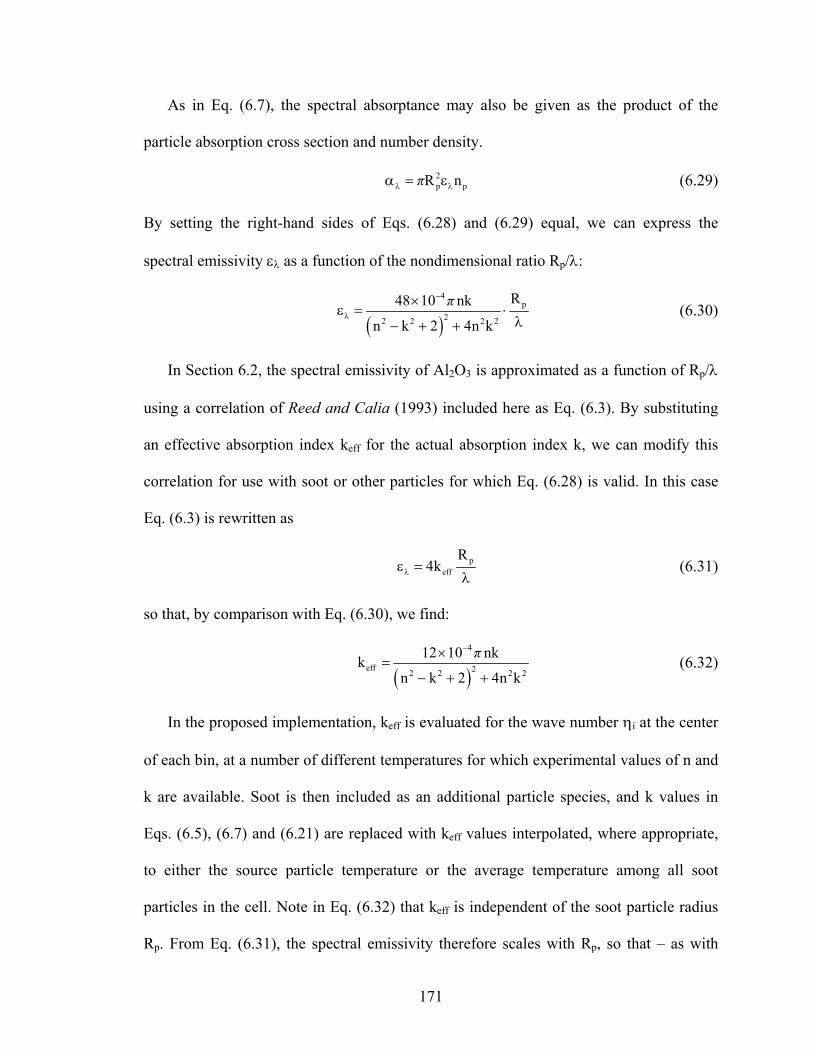
As in Eq. (6.7), the spectral absorptance may also be given as the product of the
particle absorption cross section and number density.
2pR nπλ λ pα = ε (6.29)
By setting the right-hand sides of Eqs. (6.28) and (6.29) equal, we can express the
spectral emissivity ελ as a function of the nondimensional ratio Rp/λ:
( )
4p
22 2 2 2
R48 10 nk
n k 2 4n k
π−
λ
×ε = ⋅
λ− + + (6.30)
In Section 6.2, the spectral emissivity of Al2O3 is approximated as a function of Rp/λ
using a correlation of Reed and Calia (1993) included here as Eq. (6.3). By substituting
an effective absorption index keff for the actual absorption index k, we can modify this
correlation for use with soot or other particles for which Eq. (6.28) is valid. In this case
Eq. (6.3) is rewritten as
peff
R4kλε =
λ (6.31)
so that, by comparison with Eq. (6.30), we find:
( )
4
eff 22 2 2
12 10 nkkn k 2 4n k
π−×=
− + + 2 (6.32)
In the proposed implementation, keff is evaluated for the wave number ηi at the center
of each bin, at a number of different temperatures for which experimental values of n and
k are available. Soot is then included as an additional particle species, and k values in
Eqs. (6.5), (6.7) and (6.21) are replaced with keff values interpolated, where appropriate,
to either the source particle temperature or the average temperature among all soot
particles in the cell. Note in Eq. (6.32) that keff is independent of the soot particle radius
Rp. From Eq. (6.31), the spectral emissivity therefore scales with Rp, so that – as with
171

Al2O3 particles – soot is modeled here as a volumetric emitter. [Reed and Calia (1993)]
Also note that no consideration is made for the presence of larger soot agglomerates.
While agglomerate particles are expected in the plume flows of interest, they are ignored
here due to the inherent complexity of any modeling procedures for particle-gas
interaction and radiative energy transfer involving particles of such highly nonspherical
shapes. [Simmons (2000)]
172

Chapter VII
Simulation of a Representative Plume Flow
7.1 Background and simulation setup
Several of the simulation procedures and physical models developed in previous
chapters have been evaluated through application to small-scale flows and comparison
with experimental measurements or theoretical results. These evaluations do not,
however, lead to confidence in the overall accuracy of the proposed simulation method
for the high altitude SRM plume flows of interest. To characterize the general utility of
the numerical scheme described in Chapters 2 through 6, simulation results based on this
scheme should ideally be compared to available experimental data for a high altitude
SRM exhaust plume. Such an approach is presented in the following sections.
First, a comparison is made between calculated UV radiation characteristics and
corresponding experimental measurements for a representative SRM plume flow.
Additional simulations are performed for which individual models are disabled or input
parameters are varied, in an effort to determine the importance of several physical
processes and numerical approximations on flowfield and radiation properties. Results
are presented with the general goal of quantifying the influence and interaction of various
173

phenomena, so that less uncertainty over the importance of these phenomena may exist in
future simulation efforts for similar flows.
7.1.1 Application to the BSUV-2 plume flow
For ease of comparison and to limit the required computer resources, experimental
measurements are desired for a plume flow which can be modeled through an
axisymmetric simulation. The exhaust flow should therefore be expelled through a single
nozzle, and the rocket should be oriented at a relatively small inclination to its direction
of motion. As found from an extensive literature search, the only experimental
measurements for a single-nozzle high altitude SRM plume flow in the open literature are
those of Erdman et al. (1992) described in Chapter 1. In a flight experiment termed “Bow
Shock Ultraviolet 2” (BSUV-2), onboard sensors were used to measure spectral radiance
in the near-UV range (wavelengths of 0.2 to 0.4 µm) from upper stage SRM exhaust
plumes at altitudes between roughly 100 and 120 km. The plume from the third stage
Star-27 SRM at an altitude of 114 km is used as a test case here, and while no
experimental data is available for flowfield properties, we can to a limited extent infer
overall simulation accuracy from a comparison of radiation characteristics between
numerical and experimental results.
Following previous simulations of Candler et al. (1992) for the same flow at 114 km,
we perform a series of axisymmetric simulations on a rectangular grid which extends
from 10 m upstream to 75 m downstream of the nozzle exit plane, and 30 m radially
outward from the nozzle centerline. The nozzle exit diameter is 0.78 m, and the rocket
174

surface geometry is approximated as a blunted cone-cylinder shape of length 3.1 m. The
grid geometry is shown in Fig. (7.1).
Figure 7.1. Grid geometry for simulations of the BSUV-2 flow.
7.1.2 Gas phase calculations
To account for the high degree of gas thermal nonequilibrium expected through much
of the grid domain, the direct simulation Monte Carlo (DSMC) method is used to
calculate gas properties in regions of relatively low density flow. The variable hard
sphere (VHS) collision model is employed to approximate the variation in transport
properties with temperature, and the Larsen-Borgnakke model [Bird (1994)] is used
together with a total collision energy model for the probability of inelastic collisions
[Boyd (1990)] to determine energy exchange between translational and rotational modes.
175

As discussed in Chapter 5, the gas density in plume core regions downstream of the
nozzle may be far too high to meet standard DSMC cell size requirements, so an alternate
approach for gas phase simulation must be used in these regions. The traditional
collision-limiter approach [Bartel et al. (1994)] provides a simple solution, but is
considerably less efficient and arguably less accurate than alternate methods which
involve resampling some fraction of gas particle velocities during each time step from
predetermined distribution functions. Both types of approaches can produce large
artificial diffusion errors, and tend to enforce a near-equilibrium gas velocity distribution
that may not be physically justified when cell dimensions are much greater than a mean
free path. [Breuer et al. (1995)] However, these approaches are generally far simpler to
implement than alternate methods, such as hybrid CFD/DSMC codes, for simulating
flowfields that include both continuum regions and nonequilibrium regions in which a
DSMC calculation is desired. This is particularly true for simulations involving a large
number of additional physical models, as is the case here, or those for which strong two-
way coupling may exist between continuum and nonequilibrium regions.
For simulation of the BSUV-2 flow, gas properties in the high density, near-
equilibrium plume core region are calculated using the ES-BGK particle method
presented in Chapter 5. The location of the boundary between DSMC and ES-BGK
domains is determined using a standard cutoff value (0.05) of the maximum gradient-
length local Knudsen number KnGLL given by Eq. (5.37). [Boyd, Chen and Candler
(1995)] This parameter is calculated throughout the grid for an initial simulation where
the ES-BGK scheme is applied to regions of both high and low gas density, and the ES-
BGK method is subsequently used only in regions where the condition
176

maxKnGLL<0.05 is satisfied in the initial simulation. Domains for ES-BGK and DSMC
methods are shown in Fig. (7.2). Note that nearly the entire plume region downstream of
the nozzle exit is contained within the ES-BGK domain. We expect, however, that a
larger portion of the plume would be within the DSMC domain if the grid extended
further downstream where, as described in Chapter 1, the reduced gas density should
make nonequilibrium effects more prominent.
Figure 7.2. Domains for DSMC and ES-BGK simulation methods.
7.1.3 Boundary conditions
Following simulations of Anfimov et al. (1993) for the same BSUV-2 flow, the Al2O3
particle phase is assumed to account for 30% of the mass flow rate at the nozzle exit, and
is made up of seven discrete particle sizes ranging from 0.3 to 6 µm in diameter.
Properties for each particle size are independently specified along inflow boundaries at
the nozzle exit plane. These inflow properties, as well as those of the gas, are taken from
a nozzle flow simulation by the same authors, and are identical to those used in the
177

subscale plume simulations of Chapter 4. Particle phase inflow properties are provided in
Table (4.1).
As in Chapter 4, the exhaust gas species are limited to H2, N2 and CO, with initial
mole fractions of 0.38, 0.31 and 0.31 respectively. At atmospheric inflow boundaries
shown in Fig. (7.1), the gas has mole fractions of 0.78 for N2 and 0.22 for O2, with a
temperature of 288 K, a density of 5.79×10⁻⁸ kg/m3, and a freestream Mach number of
13.5. Following the simulations of Chapter 4, a thermal accommodation coefficient of 0.9
is used for collisions between gas molecules and condensed phase particles, while the
outer surfaces of the rocket are modeled as diffusely reflecting walls at 300 K with full
thermal accommodation.
7.1.4 Plume radiation properties
In the particle radiation model presented in Chapter 6, values of the absorption index
k are calculated as a function of temperature and wavelength. Within the IR range where
most radiative energy transfer through the plume is concentrated, absorption index values
are taken from experimental measurements of Konopka, Reed and Calia (1983). Based
on this data, we use 10 wave number bins within the IR range corresponding to
wavelengths of 1.0 to 4.5 µm. Of the two SRM exhaust flows from which particles were
collected and investigated by these authors, the second (rocket 2) was found to give k
values more in line with other experimental data and correlations in the literature. [Duval,
Soufiani and Taine (2004)] Values calculated from scanning electron microscope (SEM)
measurements for the second flow are therefore used here.
178
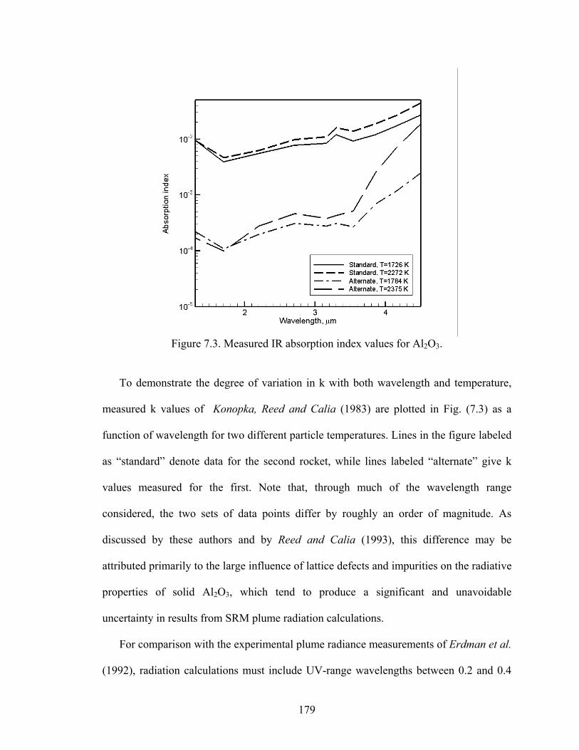
Figure 7.3. Measured IR absorption index values for Al2O3.
To demonstrate the degree of variation in k with both wavelength and temperature,
measured k values of Konopka, Reed and Calia (1983) are plotted in Fig. (7.3) as a
function of wavelength for two different particle temperatures. Lines in the figure labeled
as “standard” denote data for the second rocket, while lines labeled “alternate” give k
values measured for the first. Note that, through much of the wavelength range
considered, the two sets of data points differ by roughly an order of magnitude. As
discussed by these authors and by Reed and Calia (1993), this difference may be
attributed primarily to the large influence of lattice defects and impurities on the radiative
properties of solid Al2O3, which tend to produce a significant and unavoidable
uncertainty in results from SRM plume radiation calculations.
For comparison with the experimental plume radiance measurements of Erdman et al.
(1992), radiation calculations must include UV-range wavelengths between 0.2 and 0.4
179

µm. While very few data sets exist for Al2O3 absorption index values in this range, the
correlations employed in plume calculations of Anfimov et al. (1993) are stated as valid
over the UV wavelengths of interest. These correlations involve a summation over four
different intrinsic emission/absorption mechanisms, and as in the data of Konopka, Reed
and Calia (1983), k values here depend on both wavelength and temperature but are
independent of the particle phase composition. Plots of the UV absorption index as a
function of wavelength are shown in Fig. (7.4) for three different particle temperatures,
based on these correlations. (The two additional lines in the figure – those for constant
emissivity and constant absorption index – will be discussed in Section 7.2.)
Figure 7.4. UV absorption index values for Al2O3.
To incorporate UV radiation calculations into the plume simulation, an additional
eight wave number bins are added to cover the wavelength range between 0.2 and 1.0
µm, with most of these bins concentrated toward smaller wavelengths (0.2 to 0.4 µm) for
180

which experimental plume radiance values are available. Absorption index values over
this entire range are taken from the correlations of Anfimov et al. (1993).
For all 18 wave number bins over the wavelength range between 0.2 and 4.5 µm, the
real part n of the particle index of refraction is computed as a function of the wave
number ηi at the center of each bin through a correlation given by Duval, Soufiani and
Taine (2004)
( )5p 2 2
i i
1/21.024 1.058 5.281n 0.9904 2.02 10 T 1
1 0.00376 1 0.01225 1 321.4−
2i
⎡ ⎤= + × + + +⎢ ⎥− η − η − η⎣ ⎦
(7.1)
where the weak temperature dependence in Eq. (7.1) is neglected by assuming a particle
temperature Tp of 2000 K. Following Reed et al. (1992), the average cosine of the
scattering angle in the Henyey Greenstein scattering phase function [Everson and Nelson
(1993)] is set to g = 0.5, and an effective temperature of Tw = 1300 K is used for
searchlight emission at the nozzle exit.
7.1.5 Additional simulation parameters
Spectral radiance calculations are made for two different simulated sensors. The first
of these is positioned near the rocket surface, with its center 2 m upstream of the nozzle
exit plane and 0.6 m from the central axis. The conical viewing region has a maximum
zenithal angle of ω = 2°, and is centered along a line oriented at a 4° inclination to the
axis. The sensor position and direction are set here for comparison between calculated
radiance values and measurements taken through a periscope-mounted onboard
radiometer in the BSUV-2 flight experiment.
181

Figure 7.5. Sensor viewing regions for plume radiance calculations.
An additional simulated sensor is positioned outside the grid domain, and is used to
characterize plume emission as would be measured from ground or air-based remote
sensors. (No such measurements were made for the BSUV-2 flight.) This second sensor
is centered at a point 50 m downstream of the nozzle exit and 100 m radially outward
from the axis, with a conical viewing region oriented normal to the axis and bounded by
the zenithal angle ω = 10°. Locations and viewing regions for both sensors are shown in
Fig. (7.5). Note that, while axial symmetry must be preserved in the shape of the sensor
surfaces (both sensors are modeled as curved surfaces of revolution around the central
axis) the conical shape of the sensor viewing regions implies a lack of symmetry. The
non-axisymmetric nature of the sensor geometry is taken into account through Eq. (6.22),
by finding the cosine in three-dimensional space between the direction vector u for an
182

incoming energy bundle and an outward normal unit vector ns within the grid plane at the
sensor surface.
Calculations are run for approximately 60 hours on eight 1.4 GHz AMD Athlon
processors. Domain decomposition is used to roughly evenly divide the computational
load among all processors, and cell size, time step and numerical weights are carefully
varied throughout the grid to balance overall simulation accuracy with computational
efficiency. The unstructured grid is divided into about 87,000 triangular cells, through
which around 7.5 million DSMC gas particles and 160,000 representative Al2O3 particles
are tracked at steady state.
7.1.6 Test for grid convergence
To assure grid convergence, a second simulation is run for which all cell dimensions
are halved, and a variety of flow property values are compared between the two sets of
simulation results. The most sensitive of the properties considered – the gas translational
temperature Tt – is found to vary by no more than a few percent between simulations
using the original and refined grids. Values of Tt for both simulations are plotted in Fig.
(7.6) along a straight extraction line which runs from the midpoint along the nozzle exit
radius to a point 75 m downstream and 25 m radially outward. This extraction line runs
roughly along the gas streamline which passes half way between the nozzle lip and
central axis, and is used in subsequent sections as a convenient measure for the variation
of gas and particle properties through the plume. The location of this line is shown in Fig.
(7.7).
183

Figure 7.6. Gas translational temperature along the extraction line.
Figure 7.7. Location of the extraction line.
7.2 Simulation results
In this section, selected results from the BSUV-2 flow simulation are presented, and a
comparison is made between calculated radiance values and experimental measurements.
This comparison can, to a limited extent, be used to evaluate the overall accuracy of the
184

simulation procedures. However, the inherent uncertainty in inflow conditions and input
parameters for the radiation model, as well as a complete lack of experimental data on
flowfield properties, lead to some doubt in the adequacy of this evaluation method. As no
other experimental results are available for a similar plume flow, the comparison of UV
spectral radiance profiles presented here seems to be a reasonable, if not completely
sufficient, method by which to assess the overall accuracy of the simulation scheme.
7.2.1 Gas bulk velocity
Some general characteristics of the simulated flowfield are displayed in Fig. (7.8),
which gives a close-up view of gas bulk velocity contours and streamlines in a 10 m long
region surrounding the rocket. The figure shows a highly diffuse bow shock, with a large
boundary layer along the front portion of the rocket surface. Further downstream, a thick
mixing layer forms along the region of plume-atmosphere interaction, and a small plume
backflow region is found just upstream of the nozzle exit and within a few meters of the
rocket. Within the plume, streamlines and velocity contours show the characteristics of a
near-free expansion flow – including a complete absence of shocks – as expected for a
highly underexpanded plume at very high altitude. [Simmons (2000)] Note the well
resolved boundary between the plume and atmospheric flow regions.
185

Figure 7.8. Gas streamlines and contours of bulk velocity magnitude. Contour line values
are given in m/s.
7.2.2 Gas and particle mass density
Contours of mass density throughout the grid are shown in Fig. (7.9). Particle phase
mass density is displayed on the top half of the figure, while the lower half gives contours
of gas density. Note first that particles are only found in roughly half of the simulation
domain, as the maximum divergence angle for the particle phase is restricted by particle
mass. Within much of the region where particles are found, the particle mass density is
shown to continuously increase with distance from the axis. This trend can be explained
as follows: As described in Section 4.4, all particles are given initial trajectories between
0° and 17.2° off the centerline along inflow boundaries at the nozzle exit, where the angle
186

for each initial particle trajectory scales linearly with distance from the axis. In the plume
nearfield region just beyond the nozzle exit, particles are forced outward from the
centerline by the expanding gas. As the drag force on a particle scales with the square of
the particle diameter Dp and the particle mass is proportional to Dp3, the radial
acceleration of an individual particle in this region will vary as roughly 1/ Dp. Thus, in a
given radial plane, smaller particles will be found over a range which extends further
from the axis. As shown in the top half of Fig. (7.9), this results in a gradual decrease in
particle mass density with distance from the axis, due to the presence of a range of
particle sizes.
Figure 7.9. Contours of mass density for particle and gas. Values are shown in kg/m3.
187
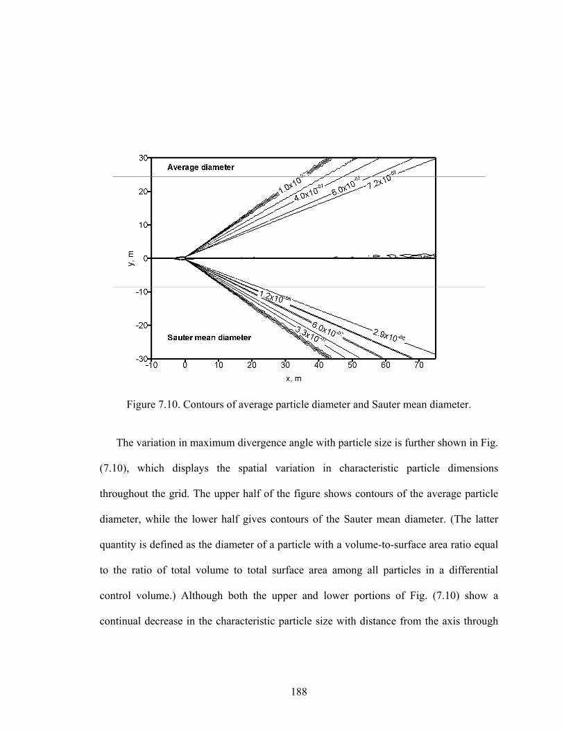
Figure 7.10. Contours of average particle diameter and Sauter mean diameter.
The variation in maximum divergence angle with particle size is further shown in Fig.
(7.10), which displays the spatial variation in characteristic particle dimensions
throughout the grid. The upper half of the figure shows contours of the average particle
diameter, while the lower half gives contours of the Sauter mean diameter. (The latter
quantity is defined as the diameter of a particle with a volume-to-surface area ratio equal
to the ratio of total volume to total surface area among all particles in a differential
control volume.) Although both the upper and lower portions of Fig. (7.10) show a
continual decrease in the characteristic particle size with distance from the axis through
188

much of the grid, the slope of this decrease is not constant due to the use of a discrete
particle size distribution.
As the dimensions of the simulation domain are about two orders of magnitude
greater than the nozzle exit radius, particle characteristics observed in both Figs. (7.9) and
(7.10) primarily reflect trends in the farfield region where interphase momentum transfer
can be assumed negligible. The particles move along nearly straight trajectories far from
the nozzle, so the contour lines shown projecting from the nozzle exit can be assumed
straight if we neglect effects of statistical scatter and interpolation between cell centers.
The continuous reduction in particle mass density with downstream distance found in
Fig. (7.9) is due to the divergence of particle trajectories, and the restricted maximum
divergence angle is shown in the figure to result in centerline values of the particle phase
mass fraction (the ratio of particle mass density to total mass density for both particles
and gas) which increase with distance from the nozzle. In comparing the upper and lower
halves of Fig. (7.9), we observe a monotonic increase in the particle mass fraction along
the central axis, with a final value 75 m downstream of the nozzle exit which is about 2.1
times greater than the initial value of 0.3.
The gas density is shown in the lower half of Fig. (7.9) to decrease continuously with
downstream distance through much of the simulation domain, as is expected for any
highly underexpanded plume flow. A sharp upward spike in gas density is observed in
the plume-atmosphere interaction region, where a diffuse shock forms as a result of both
the presence of a solid body and the convergence of streamlines between areas of
atmospheric and exhaust flows. The reduction in gas density found near the central axis is
a non-physical characteristic of axisymmetric simulations using particle methods; to
189

populate cells near the axis with a sufficient number of gas particles, the numerical
weight of particles in these regions will often need to be reduced. This in turn leads to
random walk errors, which tend to decrease the accuracy of simulation results at points
near the axis.
7.2.3 Particle temperatures
Contours of average particle temperature are shown in Fig. (7.11) for two different
sizes of Al2O3 particles. The upper half of the figure gives temperatures for 0.4 µm
diameter particles, which are toward the lower end of the particle size distribution, while
temperature contours in the lower half of the figure are for much larger particles of 4 µm
diameter. Note first the difference in the regions occupied by particles of the two
different sizes. As discussed above, smaller particles experience a greater radial
acceleration in the plume nearfield region just beyond the nozzle exit, so the maximum
divergence angle is greater for the smaller particle size. Also note that the temperature of
the smaller 0.4 µm particles is uniformly shown to be about 1200 K lower than that of the
4 µm particles. This follows primarily from the relation between particle heat capacity,
which scales as Dp3, and the convective heat transfer rate, which is proportional to Dp
2. It
can be shown from these scaling relations that the rate of change in particle temperature
tends to vary as 1/Dp, so that smaller particles will be more rapidly cooled by the
surrounding gas in the plume nearfield region where convective heat transfer is
significant.
190

Figure 7.11. Average temperature contours for 0.4 and 4 µm diameter particles. Values
are in K.
For both particle sizes in Fig. (7.11), the average temperature is generally found to
increase with distance from the central axis. This is due to the fact that, on the scale of the
simulation domain, most trends in particle temperature are dominated by the influence of
convective heat transfer. As the convective heat transfer rate is proportional to the local
gas density, we expect that particles which pass through the lower-density portions of the
plume nearfield region further from the axis will experience less heat loss to the cooler
surrounding gas. Particles further from the axis will therefore retain higher temperatures
far downstream, as is shown in the figure. The increase in particle temperatures at points
very close to the axis is also related to the radial variation in gas density within the plume
191
nearfield region. As explained in the above discussion of Fig. (7.9), random walk errors
in cells near the axis produce an artificially low gas density, which in turn reduces
convective heat transfer rates for particles which pass through these cells.
Most of the streamwise reduction in temperature shown for both particle sizes in Fig.
(7.11) is a result of radiative heat loss. Due to the large scale of the simulation domain in
relation to the size of the rocket, the regions where convective heat transfer and phase
change make significant contributions to the particle energy balance are restricted to a
small area within a few meters of the nozzle exit. A close-up view of average particle
temperatures in this area, again for particles of diameter 0.4 and 4 µm, is shown in Fig.
(7.12).
Figure 7.12. Close-up view of particle temperature contours. Values are given in K.
192

Note the contrast between Figs. (7.11) and (7.12) in the magnitude of observed
temperature variation with downstream distance for both particle sizes. Particle
temperatures are found to vary far more rapidly in the plume nearfield region displayed in
Fig. (7.12) than in regions further downstream, shown in Fig. (7.11), which make up most
of the simulation domain. This difference in temperature gradients is due primarily to the
rapid reduction in gas density with downstream distance. As shown in Fig. (7.9), the gas
density is far higher in the nearfield plume region just downstream of the nozzle than
elsewhere in the plume, so convective heat transfer rates will be far higher as well near
the nozzle exit.
7.2.4 Particle phase change
A close observation of 4 µm particle temperature contours in Fig. (7.12) reveals a
rapid temperature jump about 0.4 m downstream of the nozzle exit. This jump is
associated with the initiation of the phase change process, and results from the release of
the latent heat of fusion for liquid Al2O3. As described in Chapter 4, 4 µm particles are
assumed to be in a completely liquid state at inflow boundaries along the nozzle exit, and
are rapidly cooled by the surrounding gas until they reach the nucleation temperature (Tf
= 1930 K) for homogeneous crystallization. Once this temperature is reached, a radially
symmetric crystallization front progresses from the surface of a particle toward its center.
The heat release associated with the phase change process causes a sudden increase in
particle temperature, and this temperature increase in turn slows the progress of the
crystallization front. For some time a quasi-equilibrium state may be reached, where the
heat release during crystallization is balanced by convective and radiative heat loss, and
193

the particle maintains a nearly uniform temperature. Further downstream, as the liquid
mass fraction approaches zero and the rate of heat release is reduced, the particle
temperature again begins to decrease as observed in Fig. (7.12).
Figure 7.13. Contours of liquid mass fraction for 4 and 6 µm diameter particles.
To demonstrate the correlation between phase change and the variation in particle
temperatures, a contour plot of the liquid mass fraction is included here as Fig. (7.13).
The top half of the figure shows cell-averaged liquid mass fractions for 4 µm particles,
while the lower half gives contours for even larger particles of 6 µm diameter. (As given
in Table (4.1), most particles of smaller sizes are assumed to be in a completely solid
state at the nozzle exit, so crystallization processes occur within the plume only for the
larger particles.) A comparison of characteristics for 4 µm particles between Figs. (7.13)
194

and (7.12) shows that, as described above, the particle temperature jump about 0.4 m
downstream of the nozzle exit is accompanied by the initiation of phase change and a
rapid reduction in the liquid mass fraction. Particle temperatures level off further
downstream, as the gradient in the liquid mass fraction decreases, and the particles
ultimately approach a completely solid state.
In comparing liquid mass fraction contours for the two different particle sizes shown
in Fig. (7.13), we find that phase change begins significantly further downstream for the
larger 6 µm particles. As explained above, the rate of temperature decrease due to
convective heat transfer tends to vary as roughly the inverse of the particle diameter, so
that larger particles will experience a longer residence time in a completely liquid state
before reaching the nucleation temperature Tf at which crystallization may begin.
For both 4 and 6 µm particles, the onset of crystallization is shown in Fig. (7.13) to
occur progressively downstream for particles which move along trajectories further from
the axis. As with the radial variation in particle temperatures, this trend is a result of the
decrease in gas density with distance from the axis. Particles which pass through regions
of lower gas density will cool more slowly through convective heat transfer, so these
particles tend to reach the nucleation temperature Tf at points further downstream.
7.2.5 Convective and radiative heat transfer rates
Figure (7.14) shows the variation with downstream distance in the magnitude of mean
convective and radiative heat transfer rates, as calculated per particle and averaged over
all particle sizes. Values are extracted along a line which runs very close to the central
axis, but is sufficiently far from the axis to be relatively unaffected by random walk
195
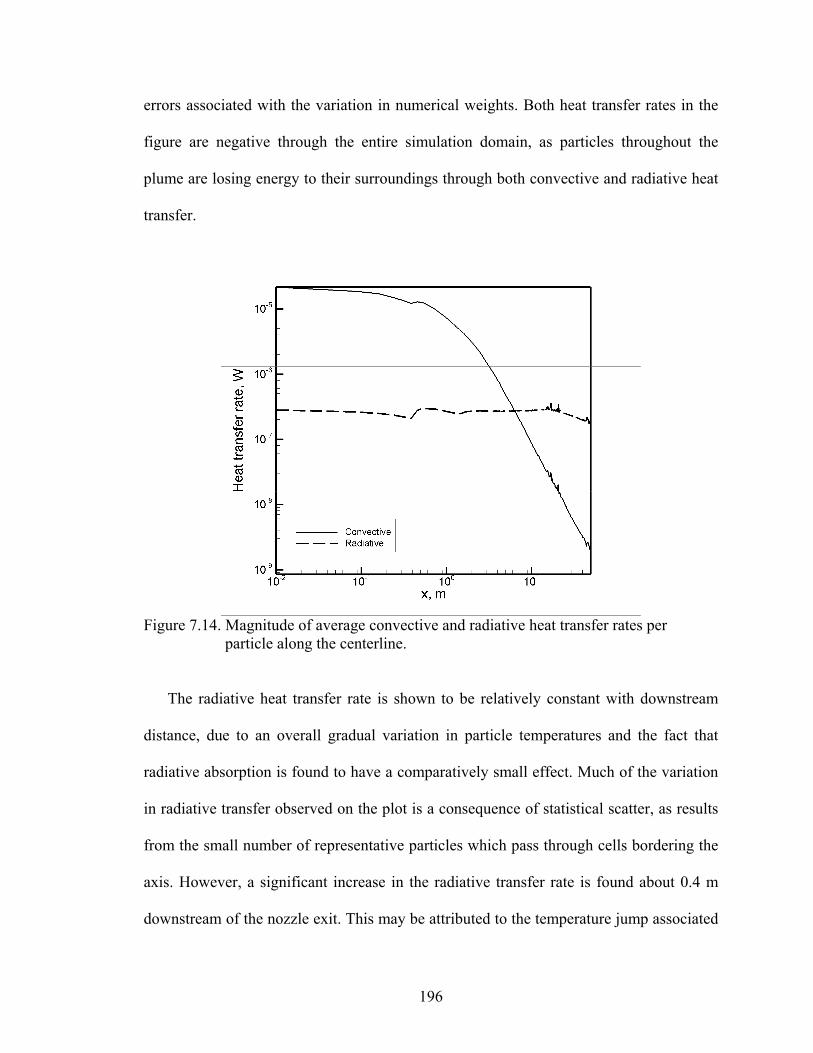
errors associated with the variation in numerical weights. Both heat transfer rates in the
figure are negative through the entire simulation domain, as particles throughout the
plume are losing energy to their surroundings through both convective and radiative heat
transfer.
Figure 7.14. Magnitude of average convective and radiative heat transfer rates per
particle along the centerline.
The radiative heat transfer rate is shown to be relatively constant with downstream
distance, due to an overall gradual variation in particle temperatures and the fact that
radiative absorption is found to have a comparatively small effect. Much of the variation
in radiative transfer observed on the plot is a consequence of statistical scatter, as results
from the small number of representative particles which pass through cells bordering the
axis. However, a significant increase in the radiative transfer rate is found about 0.4 m
downstream of the nozzle exit. This may be attributed to the temperature jump associated
196

with the onset of phase change in 4 µm particles, which account for roughly 60% of the
total Al2O3 mass within the plume.
The slow reduction in radiative heat transfer observed to begin about 10 m
downstream of the nozzle is also the result of a variation in particle temperature. As
particle temperatures decrease due to radiative heat loss in the farfield plume region, the
magnitude of the radiative energy transfer rate will decrease as well due to the strong
temperature dependence of particle emissive power.
In contrast to the relatively uniform rate of radiative heat transfer, the mean
convective heat transfer rate is shown in Fig. (7.14) to decrease rapidly with downstream
distance. The spatial variation in convective heat transfer occurs mainly as a result of the
downstream decrease in gas density. As the gas approaches a free molecular state far
from the nozzle, the gas density will decrease along the centerline as the inverse square of
the distance from the nozzle exit. The farfield convective heat transfer rate will therefore
have the same inverse square variation, as is shown in the figure.
A convenient definition of the plume nearfield region in a freely expanding SRM
plume flow is the range beyond the nozzle exit where the particle energy balance is
dominated by convective heat transfer to the gas. By this definition, the nearfield region
extends along the centerline about 6 m (or 8 nozzle exit diameters) downstream of the
nozzle exit, beyond which radiative emission becomes the dominant mechanism for
energy transfer between a particle and its surroundings.
197

7.2.6 Radiative energy flux
In Fig. (7.15), contours are shown for the direction-averaged spectral radiative energy
flux Eλ at wavelengths of 2.2 µm and 0.24 µm. This flux is defined as the rate per unit
wavelength at which photons within a narrow wavelength range impinge on a spherical
surface, divided by the cross sectional area of the sphere. Following the procedures
described in Chapter 6, Eλ may be calculated as the ratio of the energy flux qi to the
wavelength range ∆λi for a given wave number bin i.
Figure 7.15. Contours of the direction-averaged spectral energy flux at wavelengths of
2.2 µm and 0.24 µm. Values are in W/m2µm.
Note that the wavelength λ corresponding to each calculated value of Eλ is equidistant
from the wavelengths which bound the wave number bin, so λ will not exactly equal the
198

inverse of the wave number ηi at the center of this bin. In general, λ may be related to ηi
by
( )i
22i i
1
4
ηλ =
η − ∆η (7.2)
where ∆ηi is the wave number range for the given bin.
While Eλ values have little physical significance outside of the radiation model
presented in Chapter 6, contours of Eλ provide a convenient means of quantifying the
variation in spectrally resolved radiation intensity throughout the simulated flowfield.
The upper half of Fig. (7.15) can therefore be viewed as a measure of IR radiation
intensity through the grid, while the lower half shows the intensity at a representative
wavelength in the UV range. In comparing Eλ contours for the two different wavelengths,
we find that the IR radiation intensity is consistently about four orders of magnitude
greater than the UV intensity, as follows from the fact that thermal radiative emission at
the particle temperatures shown in Figs. (7.11) and (7.12) is typically concentrated in the
IR range. [Reed and Calia (1993)]
A significant difference is also found in the shape of contour lines between the two
wavelengths shown in Fig. (7.15). This difference may be attributed to the variation with
wavelength in the temperature dependence for thermal emission. At smaller wavelengths
the spectral emissive power for a blackbody tends to depend far more strongly on the
temperature of the body. [Siegel and Howell (1981)] This characteristic is preserved in
Eqs. (6.4) and (6.5), which give the emissive power output of a source particle used in the
radiation model. As shown in Fig. (7.11), particles further from the axis tend to have
higher temperatures, so experience a greater rate of radiative heat loss. This temperature
199

difference has a stronger correlation to emissive power in the UV range than in the IR
range, so a more pronounced ridge is shown in the UV energy flux contours near the
location of higher temperature particles.
As shown in Fig. (7.15), the energy flux for both wavelengths is greatest at the nozzle
exit, due primarily to the corresponding maximum in particle mass density and a
reduction in the intensity of searchlight emission with distance from the nozzle. Particles
are modeled through Eq. (6.3) as volumetric emitters [Reed and Calia (1993)], so the
magnitude of radiative energy flux should scale roughly with the local particle mass
density. As this density decreases with downstream distance due to the divergence of
particle trajectories through the plume, a continuous reduction in radiative energy flux is
found in the axial direction.
A reduction in energy flux is also observed in the radial direction, particularly outside
the region where particles are found. This follows from the fact that, in an axisymmetric
simulation, the ratio of cell volume to the projected area on the grid will scale with
distance from the axis. The average number of energy bundles which pass through a cell
is proportional to the projected area of that cell, and the contribution of each bundle to the
energy flux is proportional to the inverse of the cell volume. We therefore expect the net
energy flux through cells outside the particle domain to scale approximately with the
inverse of the distance from the axis, as is shown in both the upper and lower halves of
Fig. (7.15).
200

7.2.7 Plume spectral radiance
In Fig. (7.16) values are presented for the plume spectral radiance Ii as observed at the
onboard and remote simulated sensors shown in Fig. (7.5). Values in the figure are
averaged over results from eight different simulations. In each of these simulations the
random number generator is initialized at a different point, but all are otherwise identical.
The error bars for the onboard sensor values give 95% confidence intervals based on a
wavelength-averaged standard deviation σavg,i from the eight simulations, and show that
the stochastic nature of the radiation model produces significant scatter in these values.
Error bars for radiance values from the remote sensor are too small to include in the
figure. (The variation in scatter between the two sets of values is mainly the result of
differences in sensor surface area, viewing angle and angular resolution as shown in Fig.
(7.5).)
Figure 7.16. Spectral radiance at onboard and remote sensors.
201

To determine the height of the error bars shown in Fig. (7.16), we assume a Gaussian
distribution of radiance values among the eight simulations for each wave number bin i,
and we further assume that the ratio of the standard deviation σi to the mean radiance Ii
from the eight simulations is independent of wavelength. It follows from these
assumptions that error bars for a 95% confidence interval should be spaced a distance of
about 1.96σavg,i from the corresponding mean value Ii [Hogg and Tanis (1997)], where
σavg,i = Ii<σj/Ij> and the averaging operation <> is taken over all wave number bins.
Both data sets plotted in Fig. (7.16) display a relatively small wavelength dependence
through much of the IR range, and a sharp drop-off in the visible and UV regions. These
trends, as well as the general shape of the radiance profiles, are consistent with Planck’s
solution for the spectral distribution of blackbody emissive power. It can further be
shown through Wien’s displacement law that the wavelength of maximum radiance for
both sensors, around 0.8 µm, corresponds to a blackbody temperature of roughly 3600 K.
[Siegel and Howell (1981)] While no particles in the simulation actually reach that
temperature, we expect that, if a greater spectral resolution is used in radiation
calculations and if the wavelength dependence in particle emissivity is disabled, the
corresponding blackbody temperature would be significantly lower.
As described in Section 7.1.5, the location and orientation of the simulated onboard
sensor corresponds to that of a periscope-mounted radiometer used to measure UV
spectral radiance during the BSUV-2 flight experiment. These measured values are
presented in Fig. (7.17) along with corresponding simulation results in the wavelength
range between 0.2 and 0.4 µm. Published numerical results of Candler et al. (1992) and
Anfimov et al. (1993) are also included for comparison. Both of these previous
202

simulations employ continuum CFD methods which for this flow may be less appropriate
than the kinetic approach used here, particularly in the highly rarefied regions within the
DSMC domain shown in Fig. (7.2). Still, somewhat better agreement is found with
experiment for these results than for those from the present simulations, particularly at
wavelengths below around 0.25 µm. Note however that in the simulations of Candler et
al., particle phase enthalpies at the nozzle exit were selected for best agreement between
calculated and experimental radiance values at the 0.23 µm wavelength. This procedure
effectively rescales the UV radiance profile to match experimental results, and makes any
quantitative comparison with experiment of questionable value.
Figure 7.17. UV spectral radiance measured at the onboard sensor.
In comparing the level of agreement between the different sets of results, also note
that radiance values determined by Anfimov et al. (1993) are subject to uncertainty
associated with correlations for the particle absorption index introduced by these same
203

authors. The correlations exhibit a strong temperature and wavelength dependence that
has not been verified elsewhere in the literature, and they do not account for extrinsic
properties (such as impurity concentrations and lattice defects) that have been found to
dominate radiation characteristics of solid phase particles. [Reed and Calia (1993)] As
the same correlations are employed for the simulations presented here, the resulting
uncertainty in radiance values for both the new simulations and those of Anfimov et al.
leads to some doubt regarding the validity of using these values to assess overall
simulation accuracy.
To determine the effect of the UV absorption index correlations on radiance values,
two additional simulations are performed. In the first simulation, the absorption index is
given a constant value of 0.01 through the UV range. As shown in Fig. (7.4), this value
roughly characterizes an average of values taken from the correlations of Anfimov et al.
(1993) over a range of temperatures and wavelengths. In the second simulation the UV
absorption index is set so that, for a given particle size, the spectral emissivity ελ in the
UV range is constant. It follows from Eq. (6.3) that, for a constant emissivity, the
absorption index k in this range must be proportional to the wavelength λ. For a given
particle radius Rp, we can relate k to λ by
p
k4R
λε ⋅ λ= . (7.3)
Particles are modeled through Eq. (6.3) as volumetric emitters, so that in an
isothermal enclosure containing particles with a range of sizes, the emissive heat flux per
unit volume will scale with the mean-cubed particle radius. As this flux should also scale
with the average over all particle sizes of the quantity ελRp2, an effective emissivity
204

which is independent of the particle radius must be proportional to the ratio of the mean-
cubed radius to the mean-squared radius. This ratio is equal to one-half the Sauter mean
diameter, which may be substituted for Rp in Eq. (7.3) for use with an effective emissivity
which is independent of particle size.
Thus, to allow for values of the UV absorption index which give a uniform effective
emissivity, we assume a characteristic Sauter mean diameter of 3.2 µm (as is found
through much of the plume region occupied by particles) and use an emissivity of 0.2.
From Eq. (7.3), this corresponds to the relation k = 0.031λ. As shown in Fig. (7.4) the
resulting k values for this “constant emissivity” case are generally of the same order as
those found through the correlations of Anfimov et al. (1993), and are very much in line
with values used in the simulation involving a constant absorption index.
Radiance values from both additional simulations are shown in Fig. (7.17), and
exhibit significantly better agreement with experiment than do base simulation results.
(The term “base simulation” refers here to simulations performed using the input
parameters described in Section 7.1, including the absorption index correlations of
Anfimov et al.) In particular, the constant emissivity simulation gives excellent agreement
with the experimental data at smaller wavelengths where the correlations of Anfimov et
al. produce the greatest disagreement. While the choice of constant emissivity or
absorption index values is to some extent arbitrary, the resulting consistency with
experiment gives us some confidence in the overall accuracy of the simulations.
In drawing conclusions from the results shown in Fig. (7.17), it should be emphasized
that this comparison is in no way sufficient to validate the physical models and numerical
procedures introduced here. Although the relatively good agreement observed between
205
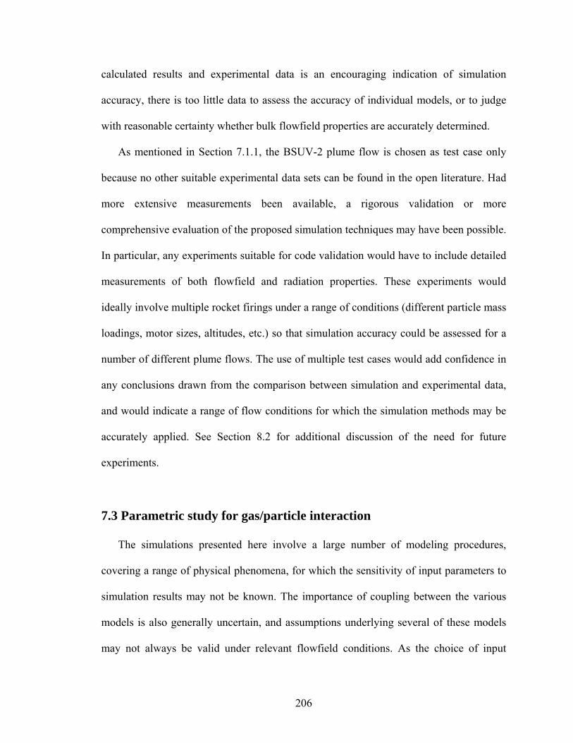
calculated results and experimental data is an encouraging indication of simulation
accuracy, there is too little data to assess the accuracy of individual models, or to judge
with reasonable certainty whether bulk flowfield properties are accurately determined.
As mentioned in Section 7.1.1, the BSUV-2 plume flow is chosen as test case only
because no other suitable experimental data sets can be found in the open literature. Had
more extensive measurements been available, a rigorous validation or more
comprehensive evaluation of the proposed simulation techniques may have been possible.
In particular, any experiments suitable for code validation would have to include detailed
measurements of both flowfield and radiation properties. These experiments would
ideally involve multiple rocket firings under a range of conditions (different particle mass
loadings, motor sizes, altitudes, etc.) so that simulation accuracy could be assessed for a
number of different plume flows. The use of multiple test cases would add confidence in
any conclusions drawn from the comparison between simulation and experimental data,
and would indicate a range of flow conditions for which the simulation methods may be
accurately applied. See Section 8.2 for additional discussion of the need for future
experiments.
7.3 Parametric study for gas/particle interaction
The simulations presented here involve a large number of modeling procedures,
covering a range of physical phenomena, for which the sensitivity of input parameters to
simulation results may not be known. The importance of coupling between the various
models is also generally uncertain, and assumptions underlying several of these models
may not always be valid under relevant flowfield conditions. As the choice of input
206

parameters and modeling approximations is of great importance in assessing the overall
accuracy of the simulation approach, we desire to evaluate the relative contributions and
interactions among a number of the modeling procedures discussed in previous chapters.
For this evaluation, results from the base simulation described above are compared with
those from a series of simulations for which individual models are turned off or input
parameters are varied. The first category of physical models and numerical
approximations to be assessed are those involved in momentum and energy exchange
between the particles and gas.
7.3.1 Additional simulations for comparison
First, the influence of momentum and energy coupling from particles to the
surrounding gas is considered by deactivating the two-way coupling model, then
performing a simulation for which gas properties are not affected by the presence of the
particle phase. The effects of particle rotation are considered next, through the activation
of models presented in Chapter 2 for the exchange of angular momentum, linear
momentum and energy between a rotating sphere and a locally free molecular
nonequilibrium gas.
Following Vasenin et al. (1995), we assume that coalescing collisions between liquid
droplets within the nozzle are the dominant contributors to particle rotation. The
maximum allowable particle angular velocity magnitude is then determined by a criterion
for the centrifugal breakup of liquid droplets. A normalized angular velocity
pp
liq
m45 3
π= ω
σΩ (7.4)
207

is set to equal some critical value Ωcrit for all particles at the nozzle exit, where mp is the
particle mass, σliq is the liquid surface tension, and ωp is the magnitude of the particle
angular velocity ωp. While ωp values will be equal for all particles of a given diameter at
the nozzle exit, the initial direction of ωp for each particle is randomly selected on a plane
normal to the central axis. Salita (1991) uses momentum and energy conservation
arguments to show that the collision-induced rotation rate of spherical liquid
agglomerates should be limited by Ωcrit=3.31. Following these arguments, we perform a
simulation for which initial particle angular velocities correspond to Ω=3.31 in order to
evaluate potential upper bounds for the influence of particle rotation on various flow
characteristics.
Another property considered here is the influence of particle shape. While Al2O3
particles extracted from SRM exhaust flows have been found to be roughly spherical,
some authors have discussed an expected deviation of particle shapes from a perfect
sphere due to surface forces on a solidifying droplet, or due to gas release during
crystallization. [Reed and Calia (1993), Gosse et al. (2003)] To quantitatively evaluate
effects of particle shape, a simulation is performed for which particles are assumed to
have the same surface area-to-volume ratio as a cube. Following the analysis in Chapter 2
of momentum and energy transfer rates between a rotating nonspherical particle and a
locally free-molecular gas, the effective particle radius and material density are modified
in order to approximate the influence of a cube-shaped surface. While this represents a
deviation from spherical shape well out of the expected range, a comparison with base
simulation results can be used to establish upper bounds for the influence of particle
shape on plume radiation and flowfield properties.
208

A final characteristic of gas-particle interaction considered here is the effect of the
thermal accommodation coefficient (TAC) at the particle surface. For all simulations
described above, the TAC value is set for all particles to 0.9, so that 90% of interphase
collisions involve diffuse reflection with full accommodation to the particle temperature,
and the remaining 10% involve specular reflection. While this TAC value is within the
general range observed experimentally [Epstein (1924)], the phenomenological nature of
the collision model and a potentially strong dependence on surface and gas properties
lead to some uncertainty over what value would be most appropriate. To assess the
influence of the TAC value on flowfield properties, an additional simulation is performed
for which the TAC is set to 0.45, so that interphase collisions are half as likely to involve
diffuse reflection as in the base simulation.
Results from these simulations are compared by evaluating flowfield properties along
the extraction line shown in Fig. (7.6). As discussed in Section 7.1.6, the extraction line
roughly follows a gas streamline originating midway between the nozzle lip and the
intersection of the central axis with the nozzle exit plane. This line is chosen to give a
general sense of the downstream variation in gas and particle properties through the
plume, while avoiding regions near the central axis which are particularly prone to effects
of random walk error and statistical scatter.
7.3.2 Gas translational temperature
In Fig. (7.18), the gas translational temperature for each of the simulations described
above is plotted as a function of distance from the nozzle exit along the extraction line.
The temperature variation with downstream distance for the base simulation shows
209

generally expected trends for a plume flow expanding into a near-vacuum: The largest
temperature gradients occur in the nearfield region just downstream of the nozzle exit,
following a rapid conversion of thermal energy into bulk kinetic energy within this
region. The rate of change decreases with downstream distance as collisional processes
become progressively less significant, and the translational temperature asymptotically
approaches a farfield value near 0 K. Note that effects of rotational freezing allow for a
potentially much higher asymptotic rotational temperature.
Figure 7.18. Gas translational temperature along the extraction line.
In comparing results with those from the base simulation, the one-way coupling case
is found to give significantly lower gas translational temperatures, particularly within the
nearfield plume region close to the nozzle exit. When the heat transfer from Al2O3
particles to the cooler surrounding gas is neglected, gas temperatures may be reduced by
well over 100 K. In contrast, the effect of particle rotation is found here to be negligible,
210

as the gas temperature is shown to be nearly identical between the base simulation and
the simulation for which particles leave the nozzle with maximum possible angular
velocities.
Particle shape is shown in Fig. (7.18) to have a potentially noticeable, although small,
influence on gas temperatures through much of the plume. When particles of fixed mass
are given greater surface area, the interphase collision frequency will increase, and higher
gas temperatures will result from a corresponding rise in convective heat transfer rates
between the particles and gas. The simulation for which the particle TAC is set to 0.45
also gives translational temperature values noticeably different from those of the base
simulation. When the probability that an interphase collision involves diffuse reflection is
halved, the heat transfer rate between the particles and gas will be reduced by roughly
50%, and particles will be considerably less effective in heating the surrounding gas. As a
result, the gas translational temperature is found to decrease by up to approximately 50 K
when the TAC is varied from 0.9 to 0.45.
7.3.3 Temperature of small particles
Average temperatures along the extraction line for 0.4 µm diameter particles are
shown in Fig. (7.19). As described in Section 7.2, the downstream reduction in particle
temperatures occurs primarily as a result of convective heat transfer in the nearfield
plume region close to the nozzle, while radiative heat transfer dominates further
downstream. In comparing results between the base simulation and the one-way coupling
simulation, for which effects on the gas of interphase momentum and energy exchange
are neglected, we find trends similar to those described above for the gas temperature. As
211
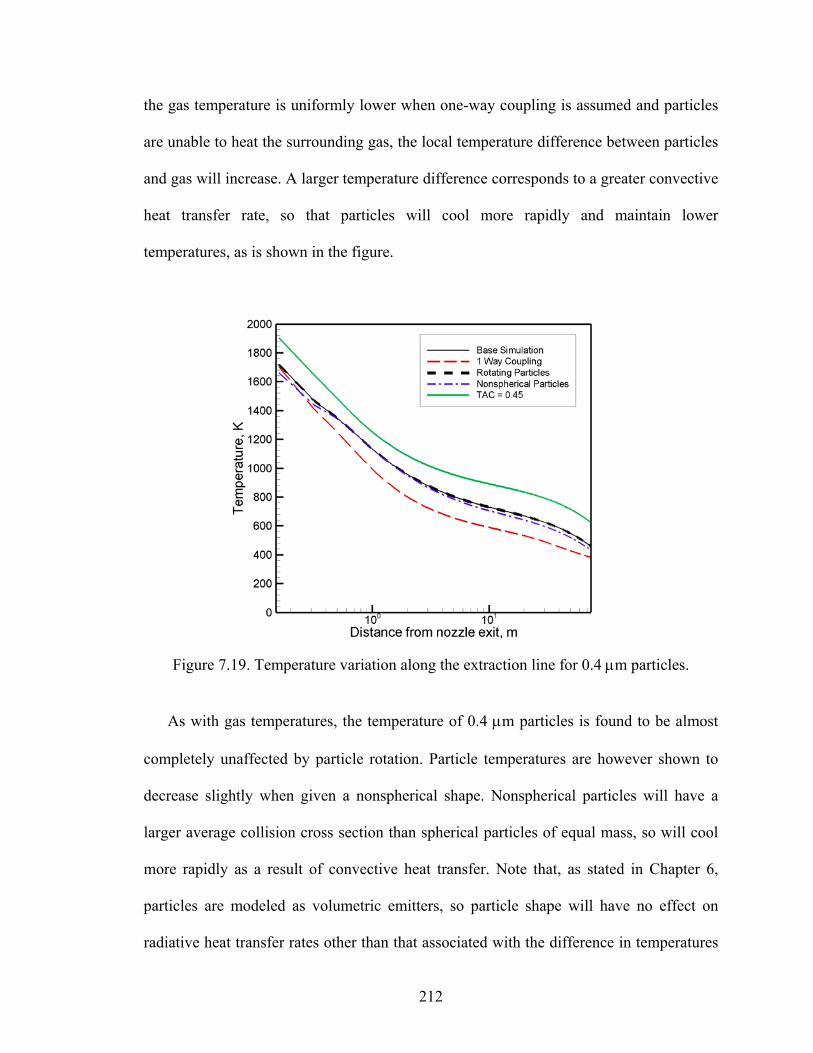
the gas temperature is uniformly lower when one-way coupling is assumed and particles
are unable to heat the surrounding gas, the local temperature difference between particles
and gas will increase. A larger temperature difference corresponds to a greater convective
heat transfer rate, so that particles will cool more rapidly and maintain lower
temperatures, as is shown in the figure.
Figure 7.19. Temperature variation along the extraction line for 0.4 µm particles.
As with gas temperatures, the temperature of 0.4 µm particles is found to be almost
completely unaffected by particle rotation. Particle temperatures are however shown to
decrease slightly when given a nonspherical shape. Nonspherical particles will have a
larger average collision cross section than spherical particles of equal mass, so will cool
more rapidly as a result of convective heat transfer. Note that, as stated in Chapter 6,
particles are modeled as volumetric emitters, so particle shape will have no effect on
radiative heat transfer rates other than that associated with the difference in temperatures
212

shown in Fig (7.19). From the temperature plot for the simulation where TAC = 0.45, we
find that the TAC value significantly influences 0.4 µm particle temperatures throughout
the plume. As convective heat transfer rates are roughly 50% lower in this simulation, the
temperature of 0.4 µm particles is found to be uniformly about 100 K higher than in the
base simulation.
7.3.4 Temperature of large particles
Figure (7.20) shows the variation along the extraction line in average temperature for
4 µm diameter particles. The non-monotonicity of all results in the figure is a
consequence of the nonequilibrium crystallization process described in Section 7.2.4, and
the general trends observed here can be explained as follows: Particles of this size are
assumed to exit the nozzle as liquid droplets. Through convective and radiative cooling,
the temperature of a droplet is ultimately reduced to a temperature (1930 K) at which
homogeneous crystallization may occur over its surface. Heterogeneous crystallization
then begins, as a crystallization front progresses toward the particle center and the
particle temperature rapidly increases due to heat release during the phase change
process. This temperature increase results in a drop in the crystallization rate, and for
some time the particle maintains a nearly constant temperature while the heat released
through crystallization is balanced by convective and radiative energy transfer. Finally, as
the liquid mass fraction approaches zero, the particle temperature again begins to
decrease due primarily to radiative heat loss.
213

Figure 7.20. Temperature variation along the extraction line for 4 µm particles.
A comparison between the base simulation results in Fig. (7.20) and those from the
other simulations shows some surprising characteristics. When the TAC is reduced,
convective heat transfer rates decrease and the location at which phase change begins is
moved further downstream. While this results in higher particle temperatures in the
farfield plume region, the delay in phase change initiation leads to significantly lower
particle temperatures in a small region upstream of the temperature spike. This region,
where a lower TAC corresponds to reduced particle temperatures, is shown in the figure
at locations between 0.5 and 1.1 m from the nozzle exit. Likewise, the increase in
convective heat transfer rates associated with both nonspherical particles and an
assumption of one-way coupling tends to force the phase change initiation point
upstream. Note however that the one-way coupling simulation gives farfield particle
214
temperatures nearly identical to those from the base simulation, while particle shape
effects are found to be potentially significant throughout the plume.
As in Figs. (7.18) and (7.19), particle rotation is shown to have no noticeable effect
here. This is in fact true of all flowfield characteristics considered, so we can conclude
that, for this flow, particle rotation has a negligible influence on all simulation results of
interest. This conclusion is however subject to assumptions regarding the mechanisms by
which particles develop angular momentum. If collisions involving partially or fully
solidified particles are considered, the appropriate value of the maximum normalized
angular velocity Ωcrit may be far higher. Higher Ωcrit values may also result from
consideration of the interaction between solid particles and either nozzle walls or large-
scale turbulent structures within the nozzle.
7.3.5 Radiative energy flux
Figure (7.21) shows the variation in net direction-averaged radiative energy flux
along the extraction line. This flux is defined as the integral of the spectral radiative
energy flux, shown in the contour plots of Fig. (7.15), over the entire wavelength range
(0.2 to 4.5 µm) considered in the radiation model. As described in the discussion of Fig.
(7.15), the radiative energy flux is found to decrease continuously with downstream
distance through the plume, primarily as a result of the divergence of particle trajectories.
The greatest variation from base simulation results is observed for the simulation with
TAC = 0.45, for which the energy flux through much of the farfield plume region is
significantly higher. Much of this increase can be attributed to the difference in
temperatures for 4 µm particles between the two simulations. These particles are shown
215

in Fig. (7.20) to experience the greatest temperature difference about 25 m downstream
of the nozzle exit. This location corresponds nearly exactly to the point in Fig. (7.21)
where the maximum difference in energy flux is observed. As 4 µm particles make up
roughly 60% of the total Al2O3 mass in the plume, and as the net emissive heat transfer
rate increases with particle temperature, this correlation between trends shown in Figs.
(7.20) and (7.21) is both logical and expected.
Figure 7.21. Net direction-averaged radiative energy flux along the extraction line.
A similar correlation between the two figures is observed in comparing results for the
base simulation and the simulation involving nonspherical particles. Spherical particles of
4 µm diameter are found in Fig. (7.20) to maintain significantly higher temperatures
through much of the plume than nonspherical particles of equal mass. This temperature
difference corresponds to a noticeable reduction in the radiative energy flux when
nonspherical particles are used. In contrast, simulations involving one-way interphase
216

coupling and rotating particles are both shown in Fig. (7.21) to give energy flux values
which are, within the scale of the figure, identical to those taken from base simulation
results.
Note in Fig. (7.20) that the variation in TAC has a significant effect on 4 µm particle
temperatures in the nearfield plume region within a few meters of the nozzle exit,
although no similar effect is found on energy flux values in this region. Nearfield
differences in the temperature of 4 µm particles when two-way coupling is disabled, or
when nonspherical particles are employed, are also not reflected in Fig. (7.21). The lack
of a correlation here between particle temperatures and energy flux is likely due to some
combination of factors: First, smaller particles cool more quickly than larger 4 µm
particles, so the relative effect of smaller particles on radiative energy flux will be greater
at locations further upstream. Second, the net radiative energy flux at any point in the
flowfield is a function of particle temperatures throughout the plume, so that
contributions to the energy flux associated with large temperature variations in the
nearfield plume region will to some extent be “smoothed out” over the length of this
region. Finally, nozzle searchlight emission is expected to have a significant influence on
the energy flux near the nozzle exit, so that Al2O3 particle emission will have a
comparatively smaller effect on flux values here than at locations further downstream.
7.3.6 UV spectral radiance
In Fig. (7.22) UV spectral radiance values at the onboard sensor are shown for the
base simulation and for all other simulations described in Section 7.3.1, and the measured
UV radiance profile from the BSUV-2 flight experiment is included here for reference.
217

Ideally a comparison of radiance values from these simulations would give us some
insight as to which numerical approximations and assumptions contribute most
significantly to the discrepancy between simulation and experimental results. However,
no clear trends are observed among the calculated radiance values, and through most of
the UV range shown here, the variation between results from the different simulations is
within the level of statistical uncertainty given by the error bars. We can at least conclude
from this comparison that none of the modeling assumptions evaluated in this section are
alone responsible for the discrepancy between experimental and calculated UV radiance
profiles.
Figure 7.22. UV spectral radiance at the onboard sensor.
7.4 Parametric study for particle radiation
In addition to numerical approximations and assumptions used for gas/particle
interaction, the overall accuracy of simulation results is subject to a number of
218

approximations in procedures for particle radiation modeling. To assess the influence of
the radiation model on output properties of interest, further simulations are performed for
which elements of flowfield-radiation coupling are disabled or input parameters for the
radiation model are modified.
7.4.1 Additional simulations
First, the influence of radiative absorption is neglected by modifying the code so that
MCRT energy bundles have no influence on the temperature of particles assigned to cells
through which the energy bundles pass. (As described in Chapter 6, each energy bundle
represents a large collection of photons over some finite wavelength range.) This in effect
decouples radiative absorption calculations from the flowfield simulation. Next, another
simulation is run using the traditional post-processing approach to plume radiation
analysis, where all radiative terms are neglected in the particle energy balance. Here both
absorption and emission are effectively decoupled from the calculation of flowfield
properties.
Results from additional simulations are used for comparison to determine the
influence of particle absorption index values on flowfield and radiation characteristics. In
one simulation, the alternate set of IR absorption index values from measurements of
Konopka et al. (1983) are used. As shown in Fig. (7.3), these values are generally about
one order of magnitude lower than those used in the base simulation, although the ratio of
corresponding values between the two data sets of Konopka et al. is a strong function of
both wavelength and particle temperature. The inclusion of both data sets should allow us
to evaluate the sensitivity of simulation results to the large inherent uncertainty in Al2O3
219

IR absorption index values. Results are also considered from the two simulations
discussed in Section 7.2.7 for which either UV absorption index or spectral emissivity
values are assumed independent of both temperature and wavelength.
Two additional simulations are included here for comparison. In the first of these, the
anisotropic scattering model employed in all other cases is disabled, and isotropic
scattering is instead assumed. (See Section 6.2.2 for a detailed description of the
scattering model.) In the second simulation, the effect of searchlight emission (i.e.
continuum radiation from the interior of the nozzle) is neglected, so that all energy
bundles used in the radiation calculations originate at source particles within the interior
of the grid.
7.4.2 Effect of particle radiation on the gas
In comparing results between all simulations for which parameters of the radiation
model are varied, we find no significant differences in gas flow properties. This is not
surprising, as the gas is assumed here to be optically transparent and may therefore be
influenced by plume radiation only indirectly through momentum and energy exchange
between the particles and gas. Radiative heat transfer is shown in Section 7.2 to
significantly affect particle properties only in the farfield plume region where interphase
momentum and energy exchange become negligible, so that plume radiation is expected
to have little if any influence on gas flow characteristics throughout the simulation
domain.
220

7.4.3 Particle temperatures
In Fig. (7.23), temperatures for 0.4 µm diameter particles along the extraction line are
compared among all simulations described in Section 7.4.1. The corresponding
temperature variation for 4 µm particles is shown in Fig. (7.24). Note that every
modification to the radiation model considered in Section 7.4.1 has virtually no effect on
particle temperatures in the plume nearfield region within a few meters of the nozzle exit.
Here radiative heat transfer has a negligible contribution to the particle energy balance,
and particle residence time in this region is too small for the emissive heat loss to have
any significant cumulative effect. Any changes to radiation input parameters or modeling
approximations should therefore have no impact on particle temperatures in this region,
as is observed in Figs. (7.23) and (7.24).
In comparing temperatures of both 0.4 µm and 4 µm particles between the base
simulation and those for which elements of flowfield-radiation coupling are disabled, we
find that radiative absorption has no significant effect on particle temperatures even in the
farfield plume region toward the downstream edge of the simulation domain. In contrast,
particle temperatures in this region may increase considerably when the contribution of
emissive heat transfer is neglected.
221

Figure 7.23. Temperature of 0.4 µm particles along the extraction line.
Figure 7.24. Temperature of 4 µm particles along the extraction line.
222

When full radiation-flowfield coupling is included and IR absorption index values are
reduced by roughly an order of magnitude to the “alternate” values of Konopka et al.
(1983), the farfield temperature for both small and large particles is shown in Figs. (7.23)
and (7.24) to increase significantly. Based on findings of Konopka et al. that the
difference between standard and alternate values plotted in Fig. (7.3) represents the
typical uncertainty in the IR absorption index range for Al2O3 particles in a SRM plume
flow, we can assume that the difference between temperature curves for the base
simulation and the simulation with alternate IR absorption index values corresponds to an
unavoidable error margin in the results.
In contrast, the use of alternate absorption index values in the UV range produces no
significant change in particle temperatures, due to the relatively small contribution of UV
emission to the total radiative heat transfer rate. Results from the simulations where
anisotropic scattering or searchlight emission are neglected also appear nearly identical to
those from the base simulation. Both searchlight emission and the angular dependence of
scattering probabilities are therefore found to have no significant influence on the
temperature of 0.4 µm or 4 µm diameter particles throughout the plume.
7.4.4 Radiative energy flux
Values of the net direction-averaged radiative energy flux are shown in Fig. (7.25) for
all simulations involving modifications to the radiation model. Note first that no
difference is observed between results from the base simulation and those from the
simulation where the influence of radiative absorption on flowfield properties is
neglected. However, a lack of radiation-flowfield coupling for both absorption and
223

emission is found to significantly increase energy flux values far downstream of the
nozzle, as results from the corresponding increase in particle temperatures shown in Figs.
(7.23) and (7.24).
Figure 7.25. Variation along the extraction line in the net direction-averaged radiative
energy flux.
The choice of values for the IR particle absorption index is found to significantly
influence energy flux values through the entire plume. When the lower “alternate” values
are used, the net energy flux is considerably reduced in both nearfield and farfield plume
regions. This is due to the fact that thermal radiative emission in the relevant temperature
range for Al2O3 particles occurs primarily at IR wavelengths. As spectral emissivity is
assumed in the radiation model to scale linearly with the absorption index, any large
change to IR absorption index values will result in a comparable change to values of the
net radiative energy flux.
224
We find no significant difference in the net energy flux when UV absorption index
values are varied, as a relatively small fraction of emissive heat loss occurs in the UV
range. A similar lack of influence on the energy flux is found in the scattering model;
results shown in Fig. (7.25) for the simulation with isotropic scattering are virtually
identical to those for the base simulation.
Nozzle searchlight emission is observed in the figure to account for over 50% of the
net radiative energy flux around the nozzle exit, while providing a negligible contribution
to flux values at distances greater than a few meters from the nozzle. Much of the
downstream reduction in the radiative energy flux within the plume nearfield region can
be attributed to the corresponding decrease in the intensity of radiation emitted inside the
nozzle. When nozzle searchlight emission is disabled, a far more gradual downstream
reduction in energy flux is found in this region.
7.4.5 UV spectral radiance
Figure (7.26) shows values of UV spectral radiance at the onboard sensor for all
simulations described in Section 7.4, and data points from the BSUV-2 flight experiment
are plotted for comparison. As mentioned in the discussion of Fig. (7.17), when either the
UV absorption index or emissivity is assumed to be independent of wavelength,
significantly better agreement is found with experimental radiance values in the 0.2 to
0.25 µm range where a particularly large discrepancy is observed between experimental
values and those from the base simulation. The simulation for which both emission and
absorption are uncoupled from flowfield calculations shows consistently higher radiance
225

values than most other simulations, as results from the corresponding increase in particle
temperatures.
Figure 7.26. Dependence of UV spectral radiance on radiation model parameters.
The level of statistical scatter in Fig. (7.26) is great enough that few definite
conclusions can be drawn from any trends observed in the figure. We do find, however,
that of all the modifications to the radiation model considered here, only adjustments to
the UV absorption index produce a statistically significant effect on calculated UV
radiance values. It follows from this comparison that most other modifications to the
radiation model cannot be assumed to measurably improve overall simulation accuracy,
to the extent that simulation accuracy is established by the level of agreement between
experiment and simulation results. Note that no broad conclusions can be drawn here for
the general application of the radiation model to high altitude SRM plume flows. If, for
example, a much larger scale plume of greater optical thickness had been considered, we
226
expect that modifications to the scattering model would have a far more significant effect
on the calculated radiance. The influence of both the scattering model and searchlight
emission would also likely be much greater if the sensor field of view were aligned more
closely to the nozzle exit plane. [Reed et al. (1992)]
7.5 Potential influence of soot on plume radiation
As discussed in Section 6.3, soot production takes place in a wide range of chemical
propulsion systems involving a hydrocarbon propellant, and is thought to occur primarily
as a result of local chemical nonequilibrium during the combustion process. While few
papers in the open literature include measurements of soot concentrations in an SRM
exhaust flow, soot has been found experimentally as an exhaust product during SRM
firings in a low density test chamber [Girata and McGregor (1983)]. In both
experimental and numerical radiation studies for liquid-propellant rocket plumes, soot is
often cited as a major contributor to plume emission characteristics. [Wright et al. (1998),
Simmons (2000), Garrison et al. (2005)]
As much uncertainty exists in the potential contribution of soot to radiation properties
for the high altitude SRM plume flows of interest, additional simulations are run for the
BSUV-2 flow in which soot is included as an additional particle species. In particular, we
hope to determine the effect of soot on calculated UV radiance values at the onboard
sensor, so that the influence of soot particles on the discrepancy between experimental
and numerical results may be quantitatively evaluated.
227

7.5.1 Soot concentration and input parameters
Based on previous simulations [Wright et al. (1998)] and experimental measurements
of soot concentrations in exhaust flows from liquid-propellant rocket engines [Simmons
(2000)], we assume a 2% mass loading of soot at the nozzle exit. Although no
corresponding data can be found for an SRM exhaust flow, the 2% value represents a
reasonable – although very rough – estimate of the expected soot concentration in the
simulated flowfield. We assume for simplicity that the soot concentration is uniform over
the nozzle exit plane, and soot particles are given initial temperatures and velocities
which are identical to those used for the gas. While noticeable soot velocity and
temperature lags may exist inside the nozzle, the very small mass and heat capacity of
soot particles allow these particles to rapidly equilibrate to local gas properties within the
plume nearfield region. The approximation of full equilibration at the nozzle exit should
therefore have little or no impact on most flowfield properties of interest.
Following the expected soot particle size distribution given by Simmons (2000), all
soot particles are given a diameter of 0.04 µm. Input parameters for the radiation model
include wavelength and temperature-dependent values of both the refractive and
absorption indices, based on an analysis of experimental data also compiled by Simmons
(2000).
Two additional simulations are performed to assess the potential influence of soot in
the BSUV-2 flow. The first simulation includes soot among the exhaust products as
described above, and is in all other ways identical to the base simulation. In the second
simulation, Al2O3 particles are entirely removed, so that the contribution of soot to plume
radiation characteristics may be independently evaluated. Note however that the second
228

simulation neglects any effects of soot absorption and scattering on radiation emitted by
Al2O3 particles, so the removal of Al2O3 particles allows for only an approximate
assessment of the influence of soot.
7.5.2 Soot density and temperature
Figure (7.27) shows contours of soot mass density and temperature throughout the
grid domain, for the simulation where both soot and Al2O3 particles are included. In
comparing soot density contours (in the upper half of the figure) to the density contours
for Al2O3 particles in Fig. (7.9), we find a significantly larger maximum divergence angle
for soot, so that soot particles are found over a larger portion of the simulated flowfield.
As explained in Section 7.2.2, smaller particles experience a greater radial acceleration
due to interphase momentum exchange in the plume nearfield region. Soot particles are
far smaller than any Al2O3 particles in the simulation, so will be deflected at potentially
much larger angles to the central axis by the rapidly expanding gas. As the gas density
through most of the plume is too low for soot particles to be noticeably accelerated far
downstream of the nozzle, these particles move along nearly ballistic trajectories through
much of the grid domain. We therefore expect a roughly inverse-square variation in soot
density with downstream distance, as is observed in Fig. (7.27). Note the similar trend in
Al2O3 particle density contours shown in Fig. (7.9).
Contours of average soot temperature are displayed in the lower half of Fig. (7.27).
First note that these temperatures are uniformly several hundred degrees lower than
Al2O3 particle temperatures shown in Fig. (7.11), as follows from the far smaller heat
capacity of soot particles and the relation between particle heat capacity and the rate of
229

convective heat transfer. (A detailed explanation of the expected temperature variation
with particle size is provided in Section 7.2.3.) As in Fig. (7.11), soot particles which
move along trajectories at large angles to the central axis are shown in Fig. (7.27) to
experience higher temperatures than particles closer to the axis, due to the reduction in
convective heat loss which results from a decrease in gas density with radial distance.
Higher temperatures are also observed for particles very close to the axis. This trend is
found in Fig. (7.11) as well, and is likely an unphysical result of inaccurate gas property
calculations near the axis. (See Sections 7.2.2 and 7.2.3 for further discussion of this
problem.)
Figure 7.27. Contours of soot mass and average temperature.
Note the spike in farfield soot temperature contours for particles with trajectories
inclined about 20° to the central axis; particles within a relatively narrow region seem to
230

cool significantly more slowly than particles with either larger or smaller divergence
angles. This difference can be attributed in part to the influence of radiative absorption.
As shown in Fig. (7.15) the magnitude of the radiative energy flux tends to be somewhat
larger near regions populated by higher temperature Al2O3 particles. This creates an
elevated level of incident radiation for soot particles which pass through regions shown in
Fig. (7.11) near the maximum divergence angle for 4 µm Al2O3 particles, and allows
these soot particles to experience an increased rate of radiative absorption. This trend can
be more clearly observed in Fig. (7.28), in which soot temperature contours are compared
between the simulation where both soot and Al2O3 particles are included, and the
simulation which includes only soot.
Figure 7.28. Contours of soot temperature for simulations with and without Al2O3
particles. Temperatures are given in K.
231

Note that the spike in farfield temperature for particles with a roughly 20° divergence
angle is completely absent in the lower half of Fig. (7.28), which shows results from the
simulation where Al2O3 particles are excluded. Soot temperatures are found to be
uniformly about 100 K lower in this second simulation, due in part to the decrease in
radiative absorption associated with the greatly reduced incident intensity when Al2O3
particles are left out of the simulation. Much of the difference in temperatures observed
between the upper and lower halves of Fig. (7.28) may also be caused by the influence of
Al2O3 particles on gas temperatures in the nearfield plume region, where significant
convective heat transfer occurs between soot particles and the gas.
7.5.3 Radiative energy flux
The variation in net radiative energy flux along the extraction line is shown in Fig.
(7.29). Results are presented here for the base simulation, the simulation involving both
soot and Al2O3 particles, and the simulation where only soot particles are included. In
comparing results between the first two simulations, we find that soot has a very small
effect on the net energy flux over the entire length of the extraction line. When soot
particles are considered independently, the total radiation intensity is found to be about
35% lower around the nozzle exit, and over two orders of magnitude lower at a distance
of about 75 m downstream.
The divergence in simulation results with downstream distance can be traced in part
to the large difference in temperature gradients between soot and Al2O3 particles, due to
convective heat transfer in the nearfield plume region. As discussed in Section 7.5.2, soot
particles will cool far more rapidly than the much larger Al2O3 particles through energy
232

exchange with the surrounding gas. Thermal radiation intensity scales with roughly the
fourth power of the source temperature, so the downstream increase in the average
temperature difference between soot and Al2O3 particles corresponds to a far larger
difference in radiation intensity contributions from the two types of particles.
Figure 7.29. Effect of soot on the net radiative energy flux along the extraction line.
Another factor in the downstream increase in differences between simulation results
shown in Fig. (7.29) is the influence of nozzle searchlight emission. As discussed in
Section 7.4.4, the contribution of searchlight emission to the radiative energy flux
decreases continuously with distance from the nozzle exit, so that particle emission,
absorption and scattering play a comparatively larger role with increasing downstream
distance. The intensity of searchlight emission is equal for all three simulations
considered here, so we expect that differences among these simulations in particle
233

radiation characteristics will result in a downstream increase in the variation between
calculated energy flux values.
7.5.4 UV spectral radiance
Figure (7.30) shows profiles of the plume UV spectral radiance, as measured at the
onboard sensor for the base simulation and the two simulations which include soot. By
comparing results from these simulations to the experimental values also shown in the
figure, we can roughly assess the expected contribution of soot to the discrepancy
between experiment and simulation results. An examination of Fig. (7.30) reveals that,
for this particular flow and for the estimated soot concentration used here, soot has no
significant influence on the calculated UV radiance values. All differences between
radiance values for the base simulation and those for the simulation involving both soot
and Al2O3 particles are within the error bars for statistical scatter, and values for the
simulation which includes only soot are uniformly over four orders of magnitude lower.
The fact that soot has such a small effect on plume UV radiance can be attributed to
the very small soot mass loading used in the simulations (less than 7% that of Al2O3
particles), and particularly to the large difference between soot and Al2O3 particle
temperatures throughout the plume. Note that thermal radiation intensity in the UV range
is particularly sensitive to source particle temperatures, while most of the radiative
energy flux throughout the simulated flowfield is concentrated at IR wavelengths where
particle radiative emission is a weaker function of temperature. The relative contribution
of soot is therefore found to be far smaller in Fig. (7.30) than in the net radiative energy
flux values displayed in Fig. (7.29).
234

Figure 7.30. Effect of soot on UV radiance at the onboard sensor.
235

Chapter VIII
Summary and Future Work
8.1 Summary
The simulation of high altitude exhaust plumes from solid propellant rockets presents
a number of modeling difficulties, and involves consideration of several complex
physical processes which are not entirely understood. The work presented in this thesis
has been performed with the goal of advancing the current state of modeling capabilities
for these flows, and assessing the relative influence and interaction between potentially
important phenomena. While the current effort does not resolve many of the known
sources of inaccuracy in the simulation of high altitude SRM plume flows, it does address
several flow physical processes that have received little previous attention in the
literature, and allows these processes to be considered together within a unified numerical
scheme.
Using the well-established DSMC method as a basis, procedures are developed here
for the integration of condensed-phase particles into the simulation of a rarefied gas flow.
We begin with the method of Gallis et al. (2001) for the determination of interphase
momentum and energy exchange rates between a locally free molecular monatomic gas
and a solid sphere. The method is extended for use with nonspherical particles or rotating
236

particles, and a further proposed modification allows for consideration of rotational
energy exchange in a diatomic gas.
Next, a series of procedures is developed for the simulation of two phase rarefied
flows involving two-way coupled momentum and energy transfer between the particles
and gas. The influence of particles on the surrounding gas is considered through Monte
Carlo procedures which involve the probabilistic modeling of individual interphase
collisions, and an alternate scheme is included for application to two-way coupled flows
involving rotating particles. A sample calculation is used to demonstrate momentum and
energy conservation in a time-averaged sense.
Following the introduction of Monte Carlo schemes for two phase flow simulation, a
set of nondimensional coupling parameters is developed for use in quantifying the effect
of interphase momentum and energy exchange. When evaluated periodically throughout
the grid, these parameters may be used to determine when a number of numerical
procedures for interphase coupling can be neglected without significantly influencing
simulation results. A model for nonequilibrium crystallization of liquid Al2O3 droplets is
presented, and is used in simulations of a subscale SRM plume flow to demonstrate the
potential efficiency benefits of simulation procedures which utilize the coupling
parameters.
One major difficulty in simulating the plume flows of interest is the enormous cost
associated with the DSMC simulation of near-equilibrium, high density regions within
the plume. We attempt to address this problem through the introduction of a new gas
simulation scheme for near-equilibrium flowfield regions. This is shown to be well suited
for integration in a DSMC code and for simulation of two phase flows using the models
237

described above. Using as a basis previous Monte Carlo methods for the ES-BGK model
of the Boltzmann equation, we develop a series of procedures which enforces momentum
and energy conservation and allows for rotational-translational energy exchange in a
diatomic gas. Homogeneous relaxation simulations are used to demonstrate that
rotational relaxation occurs at the correct rate, and the overall accuracy of the method is
assessed through simulations of a rarefied nozzle flow.
As a final addition to the proposed simulation method, a MCRT model is presented
for plume radiation analysis and for integration of radiative heat transfer effects into the
particle energy balance. Condensed phase emission, absorption and anisotropic scattering
are considered, and a model for nozzle searchlight emission is included as well. No
assumptions are made regarding plume optical thickness, although all gas species are
assumed to be optically transparent. The radiation model is fully integrated with flowfield
simulation procedures, to account for potentially significant two-way coupling between
radiation and flowfield properties. Additional procedures are described for the integration
of soot or other very small particles into the simulation.
In an effort to evaluate the overall accuracy of the proposed scheme, a series of
simulations is performed for a representative SRM plume flow. A number of simulation
results are presented, and various flowfield characteristics are discussed. Limited
comparisons are made between calculated UV radiance values and measured values from
a flight experiment. While no definite conclusions can be drawn from these comparisons,
relatively good agreement is observed between simulation and experimental results. Note
that a rigorous assessment of simulation accuracy is not possible due a lack of more
238

detailed experimental data, although the level of agreement observed here is an
encouraging indication of overall accuracy.
A series of parametric studies involving simulations of the same SRM plume flow is
used to evaluate the influence of several physical processes and input parameters. The
first of these studies considers models for gas-particle interaction. Here we find that
particle and gas temperatures through much of the plume may be significantly affected by
two-way interphase momentum and energy exchange. Values of the particle thermal
accommodation coefficient are found to greatly influence flowfield properties as well as
radiation intensity in the farfield plume region, while effects of particle rotation are
shown to be negligible.
Another parametric study examines models and parameters related to plume
radiation. In this study, we find that only the choice of particle UV absorption index
values can account for the discrepancy observed between simulation and experimental
values of plume spectral radiance in the 0.2 to 0.25 µm wavelength range. Most of the
disagreement with the experimental data can therefore be traced to a large inherent
uncertainty in the determination of absorption index values. Within the IR range, these
values are also found to strongly influence particle temperatures and net radiation
intensity through much of the plume. Nozzle searchlight emission is shown to
significantly contribute to net radiation intensity in the nearfield plume region, while
particle radiative emission – but not absorption – has a considerable effect on particle
temperatures further downstream.
In a third parametric study, we consider the potential influence of soot on plume
radiation properties. Soot is found to have a very small effect on net radiation intensity
239

throughout the plume, with a contribution relative to that of Al2O3 particles which
decreases continuously with downstream distance. As measured from a simulated
onboard sensor, UV spectral radiance values associated with soot are roughly four orders
of magnitude smaller than base simulation values, so that the presence of soot may be
safely ruled out as a significant contributor to the differences observed between
simulation results and experimental data.
8.2 Modeling difficulties and proposed future work
While it is hoped that the work introduced here represents significant progress in the
development of capabilities for high altitude SRM plume simulation, the inherent
complexity and challenges associated with these simulations leave extensive room for
future progress. A number of research areas exist for the improvement of simulation
accuracy or computational efficiency, while a sufficient evaluation of simulation
techniques likely requires that additional flight experiments be performed.
8.2.1 Unified nozzle/plume flow simulations
One important area of future work is in the development of codes and numerical
methods for the unified simulation of SRM exhaust flows, where multiphase flow
processes within the propellant grain, nozzle and plume are considered together within a
single numerical framework. As internal and external rocket exhaust flows typically
require different simulation capabilities and present different challenges, the integration
of simulation techniques valid for all flowfield regimes in high altitude SRM exhaust
flows may be a very demanding task. However, such an integrated simulation scheme
240

would allow for far more rapid, and potentially more accurate, characterization of
flowfield and radiation properties of interest. More detailed and spatially nonuniform
flow property information could be easily obtained in the region around the nozzle exit,
and two-way coupling effects between the nozzle and plume flow regions could more
simply and accurately be addressed. These coupling effects may be particularly important
for consideration of radiative heat transfer, and for accurate characterization of the
subsonic boundary layer and sonic point around the nozzle lip.
8.2.2 Monte Carlo methods for near-equilibrium flows
As discussed in Chapter 5, the wide range of the Knudsen number regimes
encountered in the flowfields of interest – from continuum to near free-molecular –
presents a particularly difficult problem in the development of a unified numerical
framework. While the DSMC method may be required to accurately simulate portions of
the plume and atmospheric flow regions, DSMC is very inefficient when applied to
higher density plume regions and is completely inappropriate for the simulation of
internal SRM exhaust flows. The use of hybrid CFD-DSMC schemes, as has been
employed in past simulation efforts for these flows [Hueser et al. (1984)], may require
the development and application of a number of compatible modeling procedures for
physical processes occurring in both continuum and rarefied flow regions. For example,
the use of separate models for radiative heat transfer and particle-gas interaction may be
needed for regions within the CFD and DSMC calculation domains.
One potentially simpler alternative to this approach is the use of alternate Monte
Carlo methods for gas phase simulation in near-equilibrium regions, as is proposed in
241

Chapter 5. The gas simulation scheme introduced here is one of a number of relatively
new particle methods for the simulation of continuum to moderately rarefied flows,
which can be easily integrated with standard DSMC to avoid many of the problems
associated with the hybrid CFD-DSMC approach. Although this and similar schemes
have been successfully applied to flowfield regimes relevant to the current effort, a few
potentially important error sources make these schemes generally unsuitable for
widespread use.
As shown by Breuer et al. (1995) for simulations employing a DSMC collision
limiter procedure, errors associated with artificial thermal equilibration tend to occur
when the cell size greatly exceeds the local mean free path. The gas thermal energy may
be partitioned nearly equally among the various translational and internal degrees of
freedom, even when this equilibration does not take place in the flow being simulated.
Given the inherent limitations of available computational resources, it is often unfeasible
to use cell dimensions on the order of a mean free path, and this artificial equilibration
effect may be unavoidable.
While the artificial equilibration error may be considerable in a moderately rarefied
flow, it does become insignificant for very low Knudsen number flows where the high
collision frequency promotes near-complete thermal equilibration. However, another
error source remains important even at the continuum flow limit. Breuer et al. (1995)
describe the numerical viscosity error which develops as a result of thermal velocity
fluctuations when cell dimensions are much larger than a mean free path. For gas
simulation techniques where particle advection and collision processes are decoupled
during each time step, and where collisional processes are not influenced by the relative
242

position of particles within a cell, it can be shown that the numerical viscosity, thermal
conductivity and mass diffusion coefficients will all scale linearly with the characteristic
cell size. As the corresponding physical transport coefficients tend to scale with the mean
free path, the ratio of numerical to physical coefficients will increase as the ratio of the
cell size to the mean free path. This may lead to large artificial diffusion errors in the
simulation of low Knudsen number flows, and tends to make these techniques generally
less accurate and practical for the characterization of high density SRM exhaust flow
regions than continuum CFD methods.
To improve overall accuracy and applicability of Monte Carlo gas simulation
techniques for continuum to moderately rarefied flows, these error sources should be
addressed. In order to reduce errors associated with artificial equilibration and numerical
diffusion, one likely direction for future work may involve the use of Brownian motion
theory to simultaneously move particles through the grid and resample particle velocities.
This avoids the approximation of temporal decoupling between advection and collision
procedures, and may reduce the dependence of various transport properties on cell size
and time step.
8.2.3 Gas radiation modeling
Other proposed areas of future work include the extension of the radiation model
presented in Chapter 6 to gas phase emission, absorption, and scattering. While the
expected contribution of gas species to radiation characteristics of most SRM plume
flows is relatively small, the inclusion of gas radiation may considerably increase the
precision and spectral resolution of plume radiance calculations. Few efforts at
243
noncontinuum gas radiation analysis through MCRT models can be found in the
literature, although procedures described by Modest (1992) seem well suited for
integration into the condensed phase radiation model presented here.
8.2.4 Radiation modeling for Al2O3 particles
Although the inclusion of gas radiation effects should improve simulation capabilities
and marginally increase the overall accuracy of radiation calculations, the uncertainty in
Al2O3 radiation characteristics far outweighs the influence of the gas. As discussed in
Chapter 7, radiative properties of Al2O3 particles are extremely complex and difficult to
model. In particular, calculations requiring spectrally resolved Al2O3 absorption and
emission characteristics are subject to significant uncertainty, due to the large number of
flowfield and material properties which must be considered for reasonably accurate
results. The spectral emissivity and absorption index of these particles has been observed
to vary as a strong function of particle size, phase composition, temperature, impurity
concentrations and the prevalence of lattice defects. [Reed and Calia (1993)]
While previous simulation efforts for similar flows have used detailed Al2O3 radiation
models which incorporate parameters not considered here [Plastinin et al. (2001)], the
inherent uncertainty in input values makes the utility of including additional parameters
seem questionable. For example, impurity concentrations may vary widely between
different SRM exhaust flows, and between different regions of the same flow. [Konopka,
Reed and Calia (1983)] Even when the strong dependence of emissive characteristics on
impurities is incorporated into the radiation model, the inherent lack of accurate input
values may lead to a large margin of error in simulation results. While no solutions to this
244

problem seem apparent, the issue is sufficiently important for the analysis of SRM plume
radiation that much further study is warranted.
8.2.5 The need for future experiments
One final proposed area of future work is the detailed experimental measurement of
both flowfield and radiation properties for a representative high altitude SRM exhaust
plume. As no such combined measurements appear to exist in the open literature, the
unavailability of experimental data makes the assessment of simulation techniques and
analysis tools extremely difficult. Although it is useful, the limited comparison with
experiment included in Chapter 7 is inadequate to sufficiently evaluate the overall
accuracy of simulation procedures presented here. A proper evaluation of these
procedures would require a more detailed comparison of simulation results with
measured flowfield and radiation characteristics. To allow for this type of comparison in
the future, additional data will be needed from either flight experiments or SRM firings in
a vacuum chamber. (Such data is in fact believed to exist in the classified literature, based
on tests conducted at the Arnold Engineering Development Center in Tennessee. A more
feasible alternative to costly experiments may therefore be a limited declassification for
some of this data.)
245

Appendices
246

Appendix A
Nomenclature
Abbreviations
BSUV-2 bow shock ultraviolet 2 flight experiment
CFD computational fluid dynamics
DSMC direct simulation Monte Carlo
ES-BGK ellipsoidal statistical Bhatnagar-Gross-Krook equation
MCRT Monte Carlo ray trace radiation model
MOC method of characteristics
NS Navier Stokes equations
NTC no time counter collision selection scheme
SRM solid rocket motor
TAC thermal accommodation coefficient
VHS variable hard sphere collision model
Symbols
A coefficient for radial distance in a least-squares fit of the particle number flux profile
247

Ac crystallization rate coefficient
Af area of a cell face
As particle surface area; surface area of a radiation sensor
cg1 gas bulk speed
cg2 root-mean-squared gas molecule speed
cnr* magnitude of non-rotational component of post-collision relative velocity
cp particle speed
cr gas molecule relative speed
cr* post-collision relative speed
(cr)max maximum pre-collision relative speed
cr1 magnitude of the difference between up and ug
cr2 average gas molecule speed relative to up
cr3 root-mean-squared gas molecule speed relative to up
cs particle specific heat
C1 cutoff value for gas-to-particle coupling
C2 cutoff value for particle-to-gas coupling
dref molecular collision diameter at the reference temperature
De distance required for an energy bundle to exit the currently assigned cell
Dp average particle diameter; distance to the surface of a radiation sensor along the direction of propagation for an energy bundle
Ds distance along energy bundle trajectory to a scattering event
Dt total distance that an energy bundle has traveled through the currently assigned cell
eint total internal energy per molecule
248

*kine post-collision gas kinetic energy
er mean rotational energy per gas molecule
E interphase energy transfer rate per unit volume
Er DSMC gas particle rotational energy
Eλ direction-averaged spectral radiative energy flux
f` gas velocity distribution function
fe equilibrium (Maxwellian) velocity distribution function
fG anisotropic Gaussian velocity distribution function
fp average interphase collision frequency per particle
fv particle phase volume fraction
Fcoll gas collision frequency
Fi net body force per unit mass
Fp force on a solid particle; particle force Green’s function
Fp,net net particle force based on Green’s function integration
Frot force Green’s function associated with particle rotation
g average cosine of the scattering angle
hf particle latent heat of fusion
Ii band-averaged spectral radiance for wave number bin i
k particle absorption index
keff effective absorption index value for soot
KnGLL gradient length local Knudsen number
L global characteristic length scale
m mass per gas molecule
249

mp particle mass
mp particle mass flux
Mp particle Mach number
Mp Green’s function for the moment on a rotating particle
Mp,net net moment on a rotating particle
n particle index of refraction
nc crystallization rate exponent
nc outward normal vector at the collision point
nf inward normal unit vector at a cell face
ng gas number density
nj time-averaged number density for particle species j
ns outward unit normal vector for a radiation sensor surface
Nb number of energy bundles created per time step
Nf number of energy bundles generated per cell face along inflow boundaries
Ng number of DSMC gas molecules in a cell
Nr number of particles selected for reassignment of rotational energy
Ns number of DSMC gas molecules selected for potential collisions; number of substeps for phase change calculations
Nspec number of different gas or particle species
Nv number of particles selected for velocity reassignment
Nη number of wave number bins
p scalar pressure
po source pressure
Pb power assigned to an energy bundle
250

Pcoll collision probability
Pp,i source particle emissive power for wave number bin i
Pr Prandtl number
P1e gas-to-particle energy coupling parameter
P1m gas-to-particle momentum coupling parameter
P2e particle-to-gas energy coupling parameter
P2m particle-to-gas momentum coupling parameter
qi direction-averaged radiative energy flux for wave number bin i
pQ particle heat transfer rate; heat transfer Green’s function
Qp,net net particle heat transfer rate based on Green’s function integration
radQ net rate of radiative heat transfer to a particle
r1 ratio of the crystallization front radius to the particle radius
R random number between 0 and 1
Rj radius for particle species j
Rp particle radius
Rs radius of the radiation sensor surface
Rt nozzle throat radius
Rw nozzle inner radius at a given axial location
Sij anisotropic Gaussian transformation matrix
So most probable gas thermal speed at the stagnation temperature
Ta(2) temperature equivalent to T(2) based on cell-averaged quantities
Teq equilibrium gas temperature based on translational and rotational temperatures
251

Tf nucleation temperature for homogeneous crystallization
Tg gas total temperature
Tj cell-averaged temperature of particle species j
Tm equilibrium melting temperature
Tp particle temperature
Tr gas rotational temperature
Tref reference temperature
Tt cell-averaged gas translational temperature
To gas stagnation temperature
T(2) gas temperature based on resampled velocities and rotational energies
u unit vector in the final direction of propagation for an energy bundle
ui point in velocity space
ug gas bulk velocity
um absolute velocity of a gas molecule
um* post-collision absolute gas molecule velocity
unr* non-rotational component of post-collision relative velocity
up particle velocity, average velocity of particles in a cell
ur gas molecule relative velocity
ur* post-collision relative velocity
urot* rotational component of post-collision relative velocity
ut tangential velocity on the particle surface
u(0) initial gas particle velocity before resampling procedures
u(1) resampled gas particle velocity
252

u(2) gas particle velocity following renormalization for momentum and energy conservation
Vc cell volume
Wg gas relative weight
Wp particle relative weight
xb location of an energy bundle
xs location of the center of a radiation sensor surface
Zr rotational collision number
αi band-averaged spectral absorptance for wave number bin i
αλ particle spectral absorptance
β inverse of gas thermal speed scale
β correction factor for the rotational relaxation rate
δ solid angle for a particle beam; collision deflection angle
ε total emissivity
εi band-averaged particle spectral emissivity for wave number bin i
ελ particle spectral emissivity
ζr number of gas rotational degrees of freedom
ζt,eff effective translational degrees of freedom
η wave number
ηi wave number at center of bin i
θ interphase collision angle; scattering angle
θv characteristic temperature of vibration
λ gas mean free path; wavelength
253

µ ratio of particle moment of inertia to that of a uniform density sphere
µ gas dynamic viscosity
µref viscosity at reference temperature
ν characteristic translational relaxation rate
νr rotational relaxation rate
ρg mass density of the gas
ρp particle material density
ρo gas stagnation density
σ logical variable for a diatomic gas; interphase collision cross section
σavg,i wavelength-averaged standard deviation of calculated spectral radiance
σi scattering coefficient for wave number bin i; standard deviation of spectral radiance
σliq liquid surface tension τ particle thermal accommodation coefficient
τcoll characteristic mean collision time
φ angle between angular velocity and relative velocity vectors
φ azimuthal angle corresponding to θ
ϕ angle between surface normal vector and ur*
χ azimuthal angle corresponding to ϕ
ψ particle shape factor
ω maximum absorption angle for a radiation sensor
ω VHS temperature exponent
ωp particle angular velocity
254

ωp angular velocity magnitude
∆qi contribution from an energy bundle to the direction-averaged radiative energy flux for wave number bin i
∆Qabs net rate of radiative energy absorption for an individual particle
∆t local DSMC time step
∆ηi wave number interval for bin i
∆λi wavelength interval for wave number bin i
Θi,j band-averaged scattering efficiency factor
ΣPi total absorbed power on a sensor surface for wave number bin i
Φ scattering phase function
Φg gas streamwise energy flux
Ψ1 logical variable for gas-to-particle coupling
Ψ2 logical variable for particle-to-gas coupling
Ωcrit critical value for the normalized angular velocity
Ωi function of temperature used to compute particle emissive power
Constants
co speed of light through a vacuum (2.99792458×10⁸ m/s)
h Planck’s constant (6.626068×10⁻³⁴ kg m2/s)
kB Boltzmann’s constant (1.3806503×10⁻²³ m2 kg s-2 K-1)
σ Stefan-Boltzmann constant (5.670×10⁻⁸ W m-2K-4)
255

Numerical operators
floor nearest smaller integer
a average over all DSMC gas particles in a cell
r average over gas particles used for rotational energy resampling
v average over gas particles used for velocity resampling
256

Appendix B
Derivation of a Formula for the Deflection Angle
A derivation is provided here for the relation between the angles θ, φ, χ, and δ given
as Eq. (3.3), based on the geometry shown in Fig. (3.1). This relation allows the
deflection angle δ in a diffusely refleccting interphase collision to be calculated as a
function of parameters which may be efficiently sampled from known distributions. First,
we define a unit vector n in the direction of the post-collision relative velocity vector ur*,
with components (nx, ny, nz) and (nx’,ny’,nz’) in the (x,y,z) and (x’,y’,z’) coordinate
systems respectively. Two additional angles must also be defined: Denote as ξ the angle
between ur* and the projection of ur
* onto the x’-y’ plane, and let ω be the angle between
this projection and the y’-axis.
The following expressions can be found for ω, χ, and ϕ in terms of the components of
the unit vector n:
tan ϕx' y'tanω = n /n 2 2x' z' y'n +n n= 2 2
x' x' z'cosχ = n n +n
Substitution then gives
tan ω = tan ϕ cos χ (B.1)
Similarly, the relations
257

sin ϕz'sin ξ = n 2 2x' z'= n +n 2 2
z' x' z'sin χ = n n +n
are used to find an expression for ξ in terms of ϕ and χ:
sin ξ = sin ϕ sin χ (B.2)
Next, δ can be related to θ, ω, and ξ by recognizing that
ycos δ = n 2 2y xcos(θ+ω) = n n +n y 2 2
x ycosξ= n +n
Then by substitution and a trigonometry identity:
cos δ = cos ξ cos (θ+ω) = cos ξ (cos θ cos ω - sin θ sin ω) (B.3)
Note that both ξ and ω are confined to the range [-π/2, π/2], hence 2cosξ= 1-sin ξ ,
, and ( 1/ 22cosω 1 tan ω−
= + ) ( ) 1/ 22sinω tanω 1 tan ω−
= + . Using these relations, Eqs. (B.1) and
(B.2) are substituted into Eq. (B.3) to give an expression for δ in terms of θ, χ, and ϕ.
After some algebraic simplification, this expression can be written as
1/ 22
2
1 (sin sin χ)cos δ (cosθ sin θ tan cos χ)
1 (tan cos χ)− ϕ
= − ϕ+ ϕ
⎡ ⎤⎢ ⎥⎣ ⎦
. (B.4)
258

Bibliography
259

Bibliography
P. Andries, J. Bourgat, P. Le Tallec, and B. Perthame. Numerical Comparison Between the Boltzmann and ES-BGK Models for Rarefied Gases. Institut National de Recherche en Informatique et en Automatique, Report No. 3872, 2000. P. Andries and B. Perthame. The ES-BGK Model Equation with Correct Prandtl Number. Proceedings of the 22nd International Symposium on Rarefied Gas Dynamics, AIP Conference Proceedings, 426-433, 2001. N. A. Anfimov, G. F. Karabadjak, B. A. Khmelinin, Y. A. Plastinin, and A. V. Rodionov. Analysis of Mechanisms and Nature of Radiation from Aluminum Oxide in Different Phase States in Solid Rocket Exhaust Plumes. AIAA Paper 93-2818, 1993. D. Baganoff and J. D. McDonald. A Collision-Section Rule for a Particle Simulation Method Suited to Vector Computers. Physics of Fluids A, 2(7):1248-1259, 1990. W. S. Bailey, E. N. Nilson, R. A. Serra, and T. F. Zupnik. Gas Particle Flow in an Axisymmetric Nozzle. ARS Journal, 793-798, June 1961. T. J. Bartel, T. M. Sterk, J. L. Payne, and P. Preppernau. DSMC Simulation of Nozzle Expansion Flow Fields. AIAA Paper 94-2047, 1994. P. L. Bhatnagar, E. O. Gross, and M. Krook. Model for Collision Processes in Gases, I. Physical Review E, 94:511, 1954. G. A. Bird. Molecular Gas Dynamics and the Direct Simulation of Gas Flows. Clarendon Press, 1994. I. D. Boyd. Analysis of Rotational Noequilibrium in Standing Shock Waves of Nitrogen. AIAA Journal, 28(11):1997-1999, 1990. I. D. Boyd. Predicting Breakdown of the Continuum Equations Under Rarefied Flow Conditions. Proceedings of the 23nd International Symposium on Rarefied Gas Dynamics, AIP Conference Proceedings, 663(1):899-906, 2003.
260

I. D. Boyd, G. Chen, and G. V. Candler. Predicting Failure of the Continuum Fluid Equations in Transitional Hypersonic Flows. Physics of Fluids, 7(1):210-219, 1995. I. D. Boyd, P. F. Penko, D. L. Meissner, and K. J. DeWitt. Experimental and Numerical Investigations of Low-Density Nozzle and Plume Flows of Nitrogen. AIAA Journal, 30(10):2453-2461, 1992. K. S. Breuer, E. S. Piekos, and D. A. Gonzales. DSMC Simulations of Continuum Flows. AIAA Paper 95-2088, 1995. D. Bruno, M. Capitelli, and S. Longo. A BGK/MC Method for the Simulation of Shock Waves in Binary Mixtures. AIAA Paper 2002-2895, 2002. D. Bruno and S. Longo. Monte Carlo Simulation of Nearly Kinematic Shock Fronts in Rarefied Gases. European Physical Journal, Applied Physics, 17:233-241, 2002. G. V. Candler, D. A. Levin, J. Brandenburg, R. Collins, P. Erdman, E. Zipf, C. Howlett. Comparison of Theory with Plume Radiance Measurements from the Bow Shock Ultraviolet 2 Rocket Flight. AIAA Paper 92-0125, 1992. C. Cercignani. The Boltzmann Equation and its Applications. Applied Mathematical Sciences, Springer Verlag, 1988. I. Chang. One and Two-Phase Nozzle Flows. AIAA Paper 80-0272, 1980. C. Chung, S. C. Kim, R. M. Stubbs, and K. J. De Witt. Low Density Nozzle Flow by the Direct Simulation Monte Carlo and Continuum Methods. Journal of Propulsion and Power, 11(1):64-70, 1995. M. S. Clark, S. C. Fisher, and E. P. French. The Flow of Very Small Alumina Particles in a Solid Rocket Plume. AIAA Paper 81-1384, 1981. C. Crowe, M. Sommerfeld, and Y. Tsuji. Multiphase Flows with Droplets and Particles. CRC Press, 1998. S. M. Dash, D. E. Wolf, R. A. Beddini, and H. S. Pergament. Analysis of Two-Phase Flow Processes in Rocket Exhaust Plumes. Journal of Spacecraft, 22(3):367-380, 1985. S. Dietrich and I. D. Boyd. Scalar and Parallel Optimized Implementation of the Direct Simulation Monte Carlo Method. Journal of Computational Physics, 126:328-342, 1996. J. Dupays. Two-phase Unsteady Flow in Solid Rocket Motors. Aerospace Science and Technology, 6(6):413-422, 2002.
261

R. Duval, A. Soufiani, and J. Taine. Coupled Radiation and Turbulent Multiphase Flow in an Aluminised Solid Propellant Rocket Engine. Journal of Quantitative Spectroscopy and Radiative Transfer, 84(4):513-526, 2004. P. S. Epstein. On the Resistance Experienced by Spheres in their Motion through Gases. Physical Review, 24:710-733, 1924. P. W. Erdman, E. Zipf, P. Espy, C. Howlett, D. A. Levin, and G. V. Candler. In-Situ Measurements of UV and VUV Radiation from a Rocket Plume and Re-entry Bow Shock. AIAA Paper 92-0124, 1992. J. Everson and H. F. Nelson. Development and Application of a Reverse Monte Carlo Radiative Transfer Code for Rocket Plume Base Heating. AIAA Paper 93-0138, 1993. J. T. Farmer and J. R. Howell. Monte Carlo Prediction of Radiative Heat Transfer in Inhomogeneous, Anisotropic, Nongray Media. Journal of Thermophysics and Heat Transfer, 8(1):133-139, 1994. H. L. Fein. A Theoretical Model for Predicting Aluminum Oxide Particle Size Distributions in Rocket Exhausts. AIAA Journal, 4(1):92-98, 1966. M. A. Gallis and J. R. Torczynski. The Application of the BGK Model in Particle Simulations. AIAA Paper 2000-2360, 2000. M. A. Gallis, J. R. Torczynski, and D. J. Rader. An Approach for Simulating the Transport of Spherical Particles in a Rarefied Gas Flow via the Direct Simulation Monte Carlo Method. Physics of Fluids, 13(11):3482-3492, 2001. M. Garrison, T. Ozawa and D. Levin. An Improved CO2, H20 and Soot Infrared Radiation Models for High Temperature Flows. AIAA Paper 2005-4777, 2005. R. L. Geisler. A Global View of the Use of Aluminum Fuel in Solid Rocket Motors. AIAA Paper 2002-3748, 2002. P. T. Girata and W. K. McGregor. Particle Sampling of Solid Rocket Motor (SRM) Exhausts in High Altitude Test Cells. AIAA Paper 83-245, 1983. S. Gosse, V. Sarou-Kanian, E. Veron, F. Millot, J. C. Rifflet, and P. Simon. Characterization and Morphology of Alumina Particles in Solid Propellant Subscale Rocket Motor Plumes. AIAA Paper 2003-3649, 2003. C. B. Henderson. Effect of Crystallization Kinetics on Rocket Performance. AIAA Journal, 15(4):600-602, 1977. R. W. Hermsen. Aluminum Oxide Particle Size for Solid Rocket Motor Performance Prediction. AIAA Paper 81-0035, 1981.
262

R. V. Hogg and E. A. Tanis. Probability and Statistical Inference. Prentice Hall, 1997. R. F. Hoglund. Recent Advances in Gas-Particle Nozzle Flows. ARS Journal, 662-671, May 1962. L. H. Holway. Kinetic Theory of Shock Structure Using an Ellipsoidal Distribution Function. Proceedings of the Fourth International Symposium on Rarefied Gas Dynamics, AIP Conference Proceedings, 193-215, 1966. J. E. Hueser, L. T. Melfi, G. A. Bird, and F. J. Brock. Analysis of Large Solid Propellant Rocket Exhaust Plumes Using the Direct Simulation Monte Carlo Method. AIAA Paper 84-0496, 1984. S. C. Hunter, S. S. Cherry, J. R. Kliegel, and C. H. Waldman. Gas-Particle Nozzle Flows with Reaction and Particle Size Change. AIAA Paper 81-0037, 1981. C. J. Hwang and G. C. Chang. Numerical Study of Gas-Particle Flow in a Solid Rocket Nozzle. AIAA Journal, 682-689, June 1988. T. Hyakutake and Kyoji Yamamoto. Numerical Simulation of Rarefied Plume Flow Exhausting from a Small Nozzle. AIP Conference Proceedings, 663(1):604-611, 2003. F. P. Incropera and D. P. DeWitt. Fundamentals of Heat and Mass Transfer. John Wiley and Sons, 1996. G. Israel and K. Friedlander. High-Speed Beams of Small Particles. Journal of Colloid and Interface Science, 24:330-337, 1967. S. G. Ivanov and A. M. Yanshin. Forces and Moments Acting on Bodies Rotating About a Symmetry Axis in a Free Molecular Flow. Fluid Dynamics, 15(3):449-453, 1980. J. H. Jeans. The Dynamical Theory of Gases. Cambridge University Press, 1916. R. M. Jenkins and R. F. Hoglund. A Unified Theory of Particle Growth in Rocket Chambers and Nozzles. AIAA Paper 69-541, 1969. T. T. Kassal. Scattering Properties of Ice Particles Formed by Release of H2O in Vacuum. Journal of Spacecraft, Vol.11(1):54-56, 1974. J. R. Kliegel and G. R. Nickerson. Flow of Gas-Particle Mixtures in Axially Symmetric Nozzles. ARS Preprint, 1715-1761, April 1961. W. L. Konopka, R. A. Reed, and V. S. Calia. Measurements of Infrared Optical Properties of Al2O3 Rocket Particles. AIAA Paper 83-1568, 1983.
263

O. B. Kovalev. Motor and Plume Particle Size Prediction in Solid Rocket Motors. Journal of Propulsion and Power, 18(6):1199-1210, 2002. D. Laredo and D. W. Netzer. The Dominant Effect of Alumina on Nearfield Plume Radiation. Journal of Quantitative Spectroscopy and Radiative Transfer, 50(5):511-530, 1993. M. N. Macrossan. A Particle Simulation Method for the BGK Equation. Proceedings of the 22nd International Symposium on Rarefied Gas Dynamics , AIP Conference proceedings, 426-433, 2001. M. N. Macrossan, M. V. Metchnik, and P. A. Pinto. Hypersonic Flow over a Wedge with a Particle Flux Method. Proceedings of the 24nd International Symposium on Rarefied Gas Dynamics , AIP Conference proceedings, 650-655, 2005. J. R. Mahan. Radiation Heat Transfer: a Statistical Approach. John Wiley and Sons, 2002. W. K. McGregor, J. A. Drakes, K. S. Beale, and F. G. Sherrell. The AlCl Absorption Feature in Solid Rocket Plume Radiation. AIAA Paper 92-2917, 1992. L. Miessens and H. Struchtrup. Numerical Comparison of Bhatnagar-Gross-Krook Models with Proper Prandtl Number. Physics of Fluids, 16(8):2797-2813, 2004. M. F. Modest. The Monte Carlo Method Applied to Gases with Spectral Line Structure. Developments in Radiative Heat Transfer, ASME HTD 203:79-84, 1992. J. M. Montanero, A. Santos, J. W. Duffy, and J. F. Lutsko. Stability of Uniform Shear Flow. Physical Review E, 57(1):546-556, 1998. F. M. Najjar, A. Haselbacher, J. P. Ferry, B. Wasistho, S. Balachandar, and R. D. Moser. Large-Scale Multiphase Large-Eddy Simulation of Flows in Solid-Rocket Motors. AIAA Paper 2003-3700, 2003. J. G. Parker. Rotational and Vibrational Relaxation in Diatomic Gases. Physics of Fluids, 2:449-462, 1959. G. N. Plass. Temperature Dependence of the Mie Scattering and Absorption Cross Sections for Aluminum Oxide. Applied Optics, 4(12):1616-1619, 1965. Y. A. Plastinin, N. A. Anfimov, G. G. Baula, G. F. Karabadzhak, B. A. Khmelinin, and A. V. Rodionov. Modeling of Aluminum Oxide Particle Radiation in a Solid Propellant Motor Exhaust. AIAA Paper 96-1879, 1996.
264

Y. A. Plastinin, G. Karabadzhak, and B. Khmelinin. Ultraviolet, Visible and Infrared Spectra Modeling for Solid and Liquid-Fuel Rocket Exhausts. AIAA Paper 2001-660, 2001. Y. A. Plastinin, H. P. Sipatchev, G. F. Karabadzhak, B. A. Knmelinin, E. Y. Szhenov, A. G. Khlebnikov, and Y. N. Shishkin. Experimental Investigation of Alumina Particles’ Phase Transition and Radiation. AIAA Paper 98-0862, 1998. D. I. Pullin. Direct Simulation Methods for Compressible Inviscid Ideal-Gas Flow. Journal of Computational Physics, 34:231-244, 1980. L. Rattenni. Solid Motor Plume Analysis for the STAR-1 Spacecraft. AIAA Paper 2000-3190, 2000. J. Reardon. Rocket Plume Base Heat Transfer Methodology. AIAA Paper 93-2823, 1993. R. A. Reed, K. S. Beale, D. W. Neese, F. G. Sherrell, D. W. Roberds, and S. M. Oliver. The Effect of Seachlight Emission on Radiation from Solid Rocket Plumes. AIAA Paper 92-2918, 1992. R. A. Reed and V. S. Calia. Review of Aluminum Oxide Rocket Exhaust Particles. AIAA Paper 93-2819, 1993. A. V. Rodionov, Y. A. Plastinin, J. A. Drakes, M. A. Simmons, and R. S. Hiers. Modeling of Multiphase Alumina-Loaded Jet Flow Fields. AIAA Paper 98-3462, 1998. D. E. Rothe. Electron-Beam Studies of Viscous Flow in Supersonic Nozzles. AIAA Journal, 9(5):804-811, 1971. M. J. Salita. Use of Water and Mercury Droplets to Simulate Al2O3 Collision/Coalescence in Rocket Motors. Journal of Propulsion and Power, 7(4):505-512, 1991. R. Siegel and J. R. Howell. Thermal Radiation Heat Transfer. McGraw-Hill, 1981. F. S. Simmons. Rocket Exhaust Plume Phenomenology. Aerospace Press, 2000. Q. Sun and I. D. Boyd. Evaluation of Macroscopic Properties in the Direct Simulation Monte Carlo Method. Journal of Thermophysics and Heat Transfer, 19(3):329-335, 2005. I. M. Vasenin, R. K. Narimanov, A. A. Glazunov, N. E. Kuvshinov, and V. A. Ivanov. Two-Phase Flows in the Nozzles of Solid Rocket Motors. Journal of Propulsion and Power, 11(4):583-592, 1995.
265

W. G. Vincenti and C. H. Kruger. Introduction to Physical Gas Dynamics. Krieger Publishing, 1986. E. I. Vitkin, V. G. Karelin, A. A. Kirillov, A. S. Suprun, and J. V. Knadyka. A Physico-Mathematical Model of Rocket Exhaust Plumes. International Journal of Heat and Mass Transfer, 40(5):1227-1241, 1997. C. Wang. Free Molecular Flow Over a Rotating Sphere. AIAA Journal, 10(5):713-714, 1972. M. J. Wright, R. M. Rao, G. V. Candler, J. S. Hong, T. A. Schilling, D. A. Levin. Modeling Issues in the Computation of Plume Radiation Signatures. AIAA Paper 98-3622, 1998. B. J. York, R. A. Lee, N. Sinha, and S. M. Dash. Progress in the Simulation of Particulate Interactions in Solid Propellant Rocket Exhausts. AIAA Paper 2001-3590, 2001.
266