MONTE CARLO SIMULATION IN DERIVATIVE

PRICING MODELS

Kai Zhang

Numerical Algorithms GroupWarwick Business School

The Thalesians Quantitative Finance SeminarCanary Wharf, London

December 15, 2009

1 / 35

Outline

Monte Carlo Overview

Monte Carlo Evolution Type

Monte Carlo for Generic SDEWiener Path GeneratorDiscretization SchemeExact Simulation

References on Monte Carlo

2 / 35

Derivative Pricing with Monte Carlo

Comparison with Lattice or PDE

1. Monte Carlo can deal with high-dimensional models.

2. Suitable for path-dependent options.

Issues

1. Different answer each simulation (supplied with standard error).

2. Slower convergence than PDE in low-dimension (1-2) case.

3. Special treatment needed for options with embedded decision.

3 / 35

Principals of Monte Carlo

Estimation of Expectation

1. Simulate a sample distribution.

2. Estimate the expectation by sample mean.

3. Estimate error bound from standard deviation.

In Derivative Pricing Models

1. Simulate a path of asset values,X = (X0, X1, · · · , XN).

2. Compute payoff from the path,V(X).

3. Compute numeraire from the path,N(X).

4. Compute option value asN0EN

(

VN

)

.

Crucial step is path simulation.

4 / 35

Monte Carlo Evolution Type I

Notations for Sample Paths

X = {Xji}

j=1,2,··· ,Mi=0,1,··· ,N

1. i is the index for time steps.

2. j is the index for sample paths.

Four Evolution Types

1. Element-wise

2. Path-wise

3. Slice-wise

4. Holistic

5 / 35

Monte Carlo Evolution Type II

Element-Wise

X10 → X1

1 → X12 · · ·X1

N → X20 → X2

1 → X22 · · ·X2

N → X30 → X3

1 · · ·

1. Low level evolution type.

2. A single value at a time.

3. Not necessarily to evolve the entire path.

4. For knock out barrier option, can stop when barrier is hit.

6 / 35

Monte Carlo Evolution Type III

Path-Wise

(X̂10, · · · , X̂1

N)↓

(X̂j0, · · · , X̂j

N)↓

(X̂M0 , · · · , X̂M

N )

1. One path at a time.

2. Suitable for path-dependent option.

3. Suitable for valuing and hedging a book of options.

4. An application is adjoint method (Giles and Glasserman (2006)).

7 / 35

Monte Carlo Evolution Type IV

Slice-Wise

X̂10...

X̂M0

→

X̂12...

X̂M2

→ · · ·

X̂1i...

X̂Mi

· · · →

X̂1N...

X̂MN

1. One slice at a time.

2. Do not always evolve forward in time.

3. Suitable for using variance reduction.

4. An example is Brownian bridge with stratified sampling.

5. Another application is Longstaff and Schwartz Monte Carlo.

8 / 35

Monte Carlo Evolution Type V

Holistic

X̂10, · · · , X̂1

N

X̂20, · · · , X̂2

N...

...X̂M

0 , · · · , X̂MN

1. The whole set of sample paths at one time.

2. Suitable when the whole set of paths is needed.

3. Variance reduction: moment matching methods.

4. Has to store everything.

9 / 35

Implementing a Monte Carlo

To Simulate a Path of Asset Value One Needs

1. A random number generator.

2. A Wiener path generator.

3. A scheme for discretizing SDE.

Simulation Procedure

1. A discrete Wiener path,W = (W0, W1, · · · , WN).

2. Back out normal variables,Zi = Wi − Wi−1, i = 1, · · · , N.

3. Choose a proper discretization scheme for SDE.

4. UseZi to construct a path for SDE,S = (S0, S1, · · · , SN).

I will talk about these in turn.

10 / 35

Wiener Path Generator I

Definition of Wiener Path

1. Independent increment:∆Wi = Wi − Wi−1, i = 1, · · · , N.

2. Gaussian increment:Wi − Wi−1 ∼ N(0,∆t).

3. Continuous int a.s.

4. W0 = 0 a.s.

Ways of Simulating a Discrete Wiener Path

1. Euler discretization.

2. Brownian bridge.

3. Spectral decomposition (do not discuss).

11 / 35

Wiener Path Generator II

Euler Discretization

1. Wi = Wi−1 +√

∆tǫi, ǫi ∼ i.i.d. N(0, 1).

2. Forward evolution,W0 → W1 → W2 → · · · → WN .

3. N multiplications andN − 1 additions.

Brownian Bridge

1. GivenWi andWk, simulateWj, i < j < k, as

Wj =

(

tk − tjtk − ti

)

Wi +

(

tj − titk − ti

)

Wk +

√

(tj − ti)(tk − tj)tk − ti

ǫ

whereǫ ∼ N(0, 1).

2. Binary chop evolutionW0 → WN → WN/2 → WN/4 → W3N/4 → WN/8 → W3N/8 · · · .

3. 3N multiplications and 2N additions.

12 / 35

Wiener Path Generator III

Sobol Brownian Bridge

1. First few draws determine the main skeleton of the Wiener path.

2. Fill the first draw (final point) with stratified samples.

3. Fill up the subsequent draws using Sobol numbers.

4. Can also use a mixture of Sobol and random numbers.

NAG Library Functions

1. FunctionG05YMF in Fortran Mark 22.

2. Generates Sobol numbers up to 50,000 dimensions.

3. Sufficient for any reasonable applications.

4. Digital scrambling Sobol generator can have standard error.

5. .DLL callable from Excel/VBA.

6. Brownian bridge is in the next release.

7. Will have GPU version of Sobol Brownian bridge.

13 / 35

Wiener Path Generator: Numerical Example

Geometric Average Rate Option

1. Option on geometric average of values at reset dates.

2. Closed-form formula (Kemma and Vorst (1990)).

Model Parameters (GBM)

1. Initial asset value,S0 = 100.

2. Constant interest rate,r = 0.05.

3. Asset volatility,σ = 0.2.

Option Parameters

1. Maturity T = 1yr.

2. StrikeX = 100.

3. Reset datesTi =i

16, i = 0, 1, · · · , 16.

14 / 35

Wiener Path Generator: Convergence Results

0 10 20 30 40 50 60 70 80 90 100−0.3

−0.2

−0.1

0

0.1

0.2

0.3

0.4

Replication

Pic

ing

Bia

s

Sobol Brownian Bridge with Different Levels of Stratifications

0 Stratification (E=3.6E−2)1 Stratification (E=5.4E−4)4 Stratifications (E=5.2E−5)16 Stratifications (E=4.2E−8)

Figure: Convergence with Different Levels of Stratifications,∆t = 1/16,EfficiencyE = SE2 × CPU, Explicit Value 5.8417

15 / 35

Wiener Path Generator: Be Aware of the Deterministic Bias

0 10 20 30 40 50 60 70 80 90 100−4

−3.5

−3

−2.5

−2

−1.5

−1

−0.5

0

0.5

1x 10

−3

Replication

Pric

ing

Bia

s

Fully Stratified Sobol Brownian Bridge

Figure: Deterministic Bias of Fully Stratified Sobol Brownian Bridge

16 / 35

Discretization Scheme I

General Asset SDE

dX = a(t, X)dt + b(t, X) · dW

1. X = (X1t , · · · , Xd

t )′ is a vector of factors.

2. W = (W1t , · · · , Wd

t )′ is d-dimensional Brownian motion.

3. a = ad×1, b = bd×d andbb′ = D, the factor covariance matrix.

Discretization

1. Chose a mesh sizeδ = maxi ∆ti.

2. ApproximateXt by its time discrete versionXδt .

3. Need Lipschitz and linear growth bound conditions ona andb.

4. Measure the closeness ofXδt to Xt by weak and strong criterions.

17 / 35

Discretization Scheme II

Weak and Strong Convergence

1. Strong convergence

E|XT − XδT | 6 Cδβ

whereδ = maxi ∆ti andC independent ofδ.

2. Weak convergence

|E[f (XT)] − E[f (XδT)]| 6 Cδβ

wheref ∈ C2(β+1) with polynomial growth.

3. β is known as the order of convergence.

We look at Euler, Milstein and higher order Itô-Taylor schemes.

18 / 35

Discretization Scheme III

Euler Scheme

X̂i+1 = X̂i + a(t, X̂i)∆t + b(t, X̂i) · ∆Wi

1. a ≡ a(t, X̂i) andb ≡ b(t, X̂i), for t ∈ [ti, ti+1].

2. O(∆t) weak convergence,O(√

∆t) strong convergence.

3. Simplest but crude.

Milstein Scheme

X̂ki+1 = X̂k

i + ak∆t +∑

l

bk,l∆W li +

∑

l,m,n

∂bk,l

∂Xn bn,mIm,l

whereIm,l =∫ ti+1

ti

∫ tti

dWms dW l

t .

1. Weak convergenceO(∆t), strong convergenceO(∆t).

2. Need evaluation ofIm,l.

19 / 35

Discretization Scheme IV

Iterated Itô Integral Im,l

1. Can show

Im,m =12

[

(∆Wmi )2 − ∆t

]

,

Im,l + Il,m = ∆Wmi ∆W l

i .

2. If∂bk,l

∂Xn bn,m =∂bk,m

∂Xn bn,l, ∀l, m, n, can takeIm,l =12∆Wm

i ∆W li .

3. For weak approximations, can approximate by moment matching

Im,l ≈ ∆Wmi ∆W l

i + Vm,l

whereP(Vm,l = ±∆t) = 12.

4. For strong approximations, see Kloeden and Platen (1999).

20 / 35

Discretization Scheme V

Strong O(∆t3/2) Itô-Taylor

∆Xi =ai∆t +∑

j

bi,j∆W j +∑

j1,j2,k

bk,j1∂bi,j2

∂Xk Ij1,j2

+∑

j

∂bi,j

∂t+

∑

k

ak∂bi,j

∂Xk +12

∑

j1,k,l

bk,j1bl,j1∂2bi,j

∂Xk∂Xl

I0,j

+∑

j,k

bk,j∂ai

∂Xk Ij,0 +12

∂ai

∂t+

∑

k

ak∂ai

∂Xk +12

∑

j,k,l

bk,jbl,j∂2ai

∂XkXl

∆t2

+∑

j1,j2,j3,k,l

bl,j1

(

∂bk,j2

∂Xl

∂bk,j3

∂Xk + bk,j2∂2bi,j3

∂Xk∂Xl

)

Ij1,j2,j3

whereIj1,j2,j3 =∫ t+∆t

t

∫ s2t

∫ s1t dW j1

u dW j2s1dW j3

s2, I0,j =∫ t+∆t

t

∫ st dudW j

s

andIj,0 =∫ t+∆t

t

∫ st dW j

uds.21 / 35

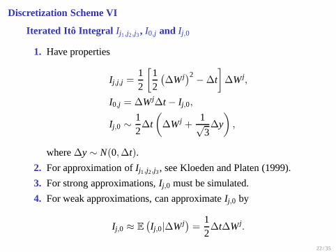
Discretization Scheme VI

Iterated Itô Integral Ij1,j2,j3, I0,j and Ij,0

1. Have properties

Ij,j,j =12

[

12

(

∆W j)2 − ∆t

]

∆W j,

I0,j = ∆W j∆t − Ij,0,

Ij,0 ∼ 12∆t

(

∆W j +1√3∆y

)

,

where∆y ∼ N(0,∆t).

2. For approximation ofIj1,j2,j3, see Kloeden and Platen (1999).

3. For strong approximations,Ij,0 must be simulated.

4. For weak approximations, can approximateIj,0 by

Ij,0 ≈ E(

Ij,0|∆W j) =12∆t∆W j.

22 / 35

Discretization Scheme VII

Weak O(∆t2) Itô-Taylor

∆Xi =ai∆t +∑

j

bi,j∆W j +∑

j1,j2,k

bk,j1∂bi,j2

∂Xk Ij1,j2

+∑

j

∂bi,j

∂t+

∑

k

ak∂bi,j

∂Xk +12

∑

j1,k,l

bk,j1bl,j1∂2bi,j

∂Xk∂Xl

I0,j

+∑

j,k

bk,j∂ai

∂Xk Ij,0 +12

∂ai

∂t+

∑

k

ak∂ai

∂Xk +12

∑

j,k,l

bk,jbl,j∂2ai

∂XkXl

∆t2

1. Do away withIj1,j2,j3.

2. I0,j ≈ Ij,0 ≈ 12∆t∆W j.

3. Ij1,j2 ≈ ∆W j1∆W j2 + Vj1,j2 whereP(Vm,l = ±∆t) = 12.

23 / 35

Discretization Scheme VIII

O(∆t) Predictor-Corrector

X̂i+1 =X̂i + [p · a(t, Xi+1) + (1− p) · a(t, X̂i)]∆t

+ [q · b(t, Xi+1) + (1− q) · b(t, X̂i)] · ∆Wi,

whereXi+1 = X̂i + a(t, X̂i)∆t + b(t, X̂i) · ∆Wi,

and

ai = ai − q∑

j,k

bj,k∂bi,k

∂Xj .

1. Easy to implement when∂bi,k

∂Xj = 0, ∀i, j, k.

2. Important scheme for LIBOR market model.

We apply various schemes to GBM and Vasicek processes.24 / 35

Discretization Scheme - GBM Example I

GBM Process

dX = rXdt + σXdW

◮ Euler scheme∆X = X(r∆t + σ∆W).

◮ Milstein scheme

∆X = X

[(

r − 12σ2

)

∆t + σ∆W +12σ2∆W2

]

.

◮ Strong O(∆t3/2) Itô-Taylor

∆X =

(

r − 12σ2

)

X∆t + σX∆W +12σ2X∆W2 +

16σ3X∆W3

+12

r2X∆t2 + (r − 12σ2)σX∆W∆t.

25 / 35

Discretization Scheme - GBM Example II

GBM Process

dX = rXdt + σXdW

◮ Weak O(∆t2) Itô-Taylor

∆X = X

[(

r +12

r2∆t − 12σ2

)

∆t + σ(1 + r∆t)∆W +12σ2∆W2

]

.

◮ O(∆t) Predictor-Corrector

∆X = X +[

1 + p(r − qσ2)∆t + qσ∆W]

X − qσ2X∆t,

whereX = X(1 + r∆t + σ∆W).

26 / 35

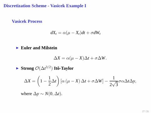
Discretization Scheme - Vasicek Example I

Vasicek Process

dXt = α(µ − Xt)dt + σdWt

◮ Euler and Milstein

∆X = α(µ − X)∆t + σ∆W.

◮ Strong O(∆t3/2) Itô-Taylor

∆X =

(

1− 12∆t

)

[α (µ − X)∆t + σ∆W] − 1

2√

3σα∆t∆y,

where∆y ∼ N(0,∆t).

27 / 35

Discretization Scheme - Vasicek Example II

Vasicek Process

dXt = α(µ − Xt)dt + σdWt

◮ Weak O(∆t2) Itô-Taylor

∆X =

(

1− 12α∆t

)

[α (µ − X)∆t + σ∆W] .

◮ O(∆t) Predictor-Corrector

∆X = (1− pα∆t)X,

whereX = X + α(µ − X)∆t + σ∆W.

28 / 35

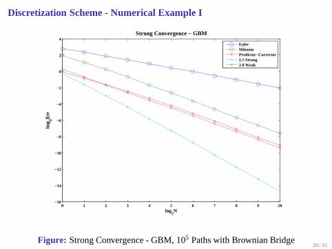
Discretization Scheme - Numerical Example I

0 1 2 3 4 5 6 7 8 9 10−16

−14

−12

−10

−8

−6

−4

−2

0

2

4

log2N

log

2Err

Strong Convergence − GBM

EulerMilsteinPredictor−Corrector1.5 Strong2.0 Weak

Figure: Strong Convergence - GBM, 105 Paths with Brownian Bridge29 / 35

Discretization Scheme - Numerical Example II

0 1 2 3 4 5 6 7 8 9 10−20

−15

−10

−5

0

5

10

log2N

log 2E

rr

Weak Convergence − GBM

EulerMilsteinPredictor−Corrector1.5 Strong2.0 Weak

Figure: Weak Convergence - GBM, 105 Paths with Brownian Bridge, WeakFunctionf = [XT − E(XT)]2

30 / 35

Discretization Scheme - Numerical Example III

0 1 2 3 4 5 6 7 8 9 10−40

−35

−30

−25

−20

−15

−10

log2N

log 2E

rr

Strong Convergence − Vasicek

Euler (Milstein)1.5 Strong2.0 WeakPredictor−Corrector

Figure: Strong Convergence - Vasicek, 105 Paths with Brownian Bridge31 / 35

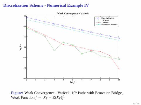
Discretization Scheme - Numerical Example IV

0 1 2 3 4 5 6 7 8 9 10−45

−40

−35

−30

−25

−20

−15

log2N

log 2E

rr

Weak Convergence − Vasicek

Euler (Milstein)1.5 Strong2.0 WeakPredictor−Corrector

Figure: Weak Convergence - Vasicek, 105 Paths with Brownian Bridge,Weak Functionf = [XT − E(XT)]2

32 / 35

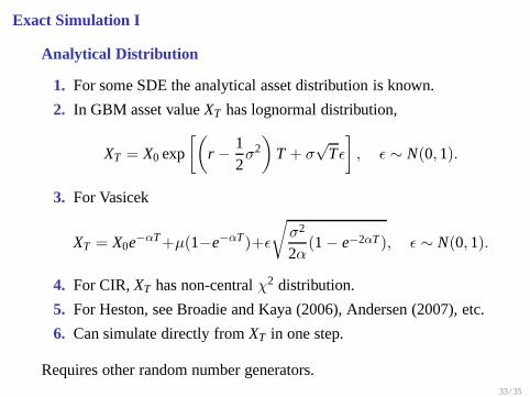
Exact Simulation I

Analytical Distribution

1. For some SDE the analytical asset distribution is known.

2. In GBM asset valueXT has lognormal distribution,

XT = X0 exp

[(

r − 12σ2

)

T + σ√

Tǫ

]

, ǫ ∼ N(0, 1).

3. For Vasicek

XT = X0e−αT +µ(1−e−αT)+ǫ

√

σ2

2α(1− e−2αT), ǫ ∼ N(0, 1).

4. For CIR,XT has non-centralχ2 distribution.

5. For Heston, see Broadie and Kaya (2006), Andersen (2007), etc.

6. Can simulate directly fromXT in one step.

Requires other random number generators.33 / 35

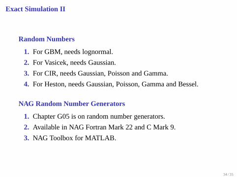
Exact Simulation II

Random Numbers

1. For GBM, needs lognormal.

2. For Vasicek, needs Gaussian.

3. For CIR, needs Gaussian, Poisson and Gamma.

4. For Heston, needs Gaussian, Poisson, Gamma and Bessel.

NAG Random Number Generators

1. Chapter G05 is on random number generators.

2. Available in NAG Fortran Mark 22 and C Mark 9.

3. NAG Toolbox for MATLAB.

34 / 35

References on Monte Carlo

Monte Carlo in Finance

1. Peter Jäckel (2002), a good introduction.

2. Paul Glasserman (2003), deeper in theory.

Discretization SchemesKloeden and Platen (1999), numerical solutions of SDE.

Computation

1. Mark Joshi (2008), a good introduction on C++ OOP.

2. Nick Webber (Wiley forthcoming), more on OOP C++ and VBA.

3. NAG library documentation on Monte Carlo components.

Benchmark with Closed-Form Formulae

1. NAG library Chapter S30 (Black-Scholes, Merton, Heston, etc).

2. Available in NAG Fortran Mark 22 and C Mark 9.

35 / 35