monte carlo simulation algorithms for the pricing of american options
TRANSCRIPT

Monte Carlo simulation algorithmsfor the pricing of American options
�Peter BQ Lin
Lady Margaret Hall
University of Oxford
A dissertation submitted for the degree of
Masters of Science
Trinity 2008

Acknowledgements
Peter BQ Lin is grateful for the support and guidance that Professor Mike
Giles has provided in the duration of the dissertation.

Abstract
One looks at the pricing of American options using Monte Carlo simula-
tions. The selected theories on the low-biased and high-biased algorithms
are reviewed. Numerical results from the implementations of the chosen
algorithms are presented and analysed. One also investigates the effects of
applying antithetic variables to the high-biased algorithm, showing that
the variance reducing technique provides great improvements to the ex-
isting algorithm.
Contents
1 Introduction 1
2 Theory on Monte Carlo pricing methods for American options 4
2.1 Problem formulation . . . . . . . . . . . . . . . . . . . . . . . . . . . 4
2.1.1 General formulation . . . . . . . . . . . . . . . . . . . . . . . 4
2.1.2 Dynamic programming formulation . . . . . . . . . . . . . . . 6
2.2 Low-biased estimators . . . . . . . . . . . . . . . . . . . . . . . . . . 8
2.2.1 Longstaff-Schwartz algorithm . . . . . . . . . . . . . . . . . . 10
2.2.2 Alternative low-biased estimator . . . . . . . . . . . . . . . . . 11
2.3 High-biased estimator . . . . . . . . . . . . . . . . . . . . . . . . . . . 12
2.3.1 Dual problem . . . . . . . . . . . . . . . . . . . . . . . . . . . 13
2.3.2 Martingales for the high estimate algorithm . . . . . . . . . . 15
3 Implementation and numerical results 17
3.1 Low-biased estimates . . . . . . . . . . . . . . . . . . . . . . . . . . . 18
3.1.1 Some analysis on the results . . . . . . . . . . . . . . . . . . . 19
3.1.2 Sources of errors of the estimates . . . . . . . . . . . . . . . . 20
3.2 High-biased estimate . . . . . . . . . . . . . . . . . . . . . . . . . . . 22
3.2.1 Results for two different numbers of sub-paths . . . . . . . . . 22
3.2.2 Antithetic variables . . . . . . . . . . . . . . . . . . . . . . . . 23
4 Summary and concluding comments 26
A Appendix 29
A.1 The implementation of Longstaff-Schwartz algorithm . . . . . . . . . 29
A.2 The implementation for the alternative low-biased algorithm . . . . . 33
i

A.3 The implementation of high-biased algorithm . . . . . . . . . . . . . . 35
Bibliography 40
ii

List of Figures
2.1 Optimal exercise boundary for a vanilla American put. . . . . . . . . 6
3.1 Vanilla American priced by the penalty method with 10000 time steps 17
3.2 Compare low-biased estimates with FD estimates . . . . . . . . . . . 20
3.3 The effects of varying the number of time steps and the number of
basis functions on the low-biased estimates . . . . . . . . . . . . . . . 21
3.4 High-biased estimates for American puts using different numbers of
sub-paths . . . . . . . . . . . . . . . . . . . . . . . . . . . . . . . . . 24
iii
Chapter 1
Introduction
What differs American-style options from European-style options is that the latter
can only be exercised at one single fixed date, i.e. the maturity date of the option,
whereas the former can be exercised any time up to the maturity. This difference
has made American options more difficult to price that European ones. For the
valuation of the European contracts, it is sufficient to take the expectations of the
discounted payoffs at the contracts’ maturities, since one can only exercise at the
terminal dates. For the American contracts, the problems of what the best excise
strategies are needs to be considered before the valuations can be done. One type
of the more simple American options is the vanilla American call with no dividends,
whose optimal exercising time is the maturity date, making it to have the same value
as its European counterpart. Apart from this simple case, the optimal exercising
time for most of American options are never this trivial. This embedded optimisation
problem that needs to be addressed, makes American options being valuated in more
complex approaches.
One type of numerical methods being successfully applied to the valuation of
American options is through the finite difference approach. This involves treating
the valuation as a linear complementarity problem. It then solves the numerical
PDEs, that the options follow, backwards in time from the maturity date. The linear
complementarity problem that uniquely determines the price of a simple American
1

options, V (S, t), is in the form of
LV (S, t) ≥ 0 (1.1)
V (S, t) ≥ h(S, t)
LV (S, t) · (V (S, t)− h(S, t)) = 0,
where h(S, t) is the payoff at time t with underlying asset S and
LV (S, t) =∂V
∂t− 1
2σ2S2∂2V
∂S2− rS
∂V
∂S+ rV,
is the classic Black-Scholes operator function. The details on different algorithms for
this approach are discussed in Chapter 27 and 28 of [5]. The finite difference approach
is very efficient for valuating American options in low dimensions, producing estimates
with high degrees of accuracies. Its computing speed however suffers greatly due to
the “curse of dimensionality” when it is applied to products with high dimensions. An
example of these is the valuation of fixed income contracts under the LIBOR market
model. Consequently, practical applications of finite difference approach is limited to
low dimensional problems.
As Monte Carlo simulations are not affected by the “curse of dimensionality”,
American option pricing methods of this kind have been looked at and developed in
recent years. Bossaerts in [1] and Tilley in [11] were among the first in attempting
to value the American options using simulation methods. One class of techniques
is based on the ideas proposed by Carriere in [3], Longstaff and Schwartz in [9] and
Tsitsiklis and Van Roy in [12, 13]. It approximates the values by formulating the
problem through dynamic programming and using regression to approximate contin-
uation values, which are the prices for holding on to contracts instead of exercising
them at exercise dates. The aim of this dissertation is to investigate the algorithms
that adopt this approach.
Three different algorithms will be assessed. As the estimators for Monte Carlo
simulation algorithms are biased in valuing the American contracts, two low-biased
algorithms and one high-biased algorithm are being considered. The low-biased algo-
rithms are the Longstaff-Schwartz algorithm, which was proposed by Longstaff and
Schwartz in [9], and an alternative low-biased algorithm based on a sub-optimal ex-
ercising policy. The high-biased algorithm originates from dual formulations, which
2

were first established by Haugh and Kogan in [8] and Rogers in [10] as a minimisation
problem. The main feature in this algorithm is the use of sub-paths in approximating
a certain type of conditional expectations required for the valuation. For the imple-
mentation of any algorithm, the accuracies of the estimates are always affected by
different sources of limitations present in practice. For all Monte Carlo simulations,
the limitation on the number of samples that can be taken causes variations within
the estimates. This dissertation also presents the other sources of limitations inherent
in these algorithms, as well as testing the effects that the limitations can have on the
estimates. It also applies a variance reducing technique to the high-biased algorithm.
The resulting estimates achieve the same accuracies as the original algorithm, which
requires 5 times the length of the former’ computational time.
The dissertation is organised as follows. Chapter 2 gives a review of the relevant
theories that the algorithms are based upon, as well as the actual details on the
algorithms. In Chapter 3, one presents and analyses the numerical results from the
implementation of these algorithms to price vanilla American put options. The results
from applying antithetic variables are also shown and compared in that chapter.
Chapter 4 is the final chapter that summaries the findings from the dissertation and
suggests plausible extensions that can be done on this dissertation.
3
Chapter 2
Theory on Monte Carlo pricingmethods for American options
This chapter presents some of the basic theories behind the different algorithms for
pricing American-style contracts. This is done in order to demonstrate how and
why the algorithms work before presenting results of the implementations. First,
the American pricing problem is formulated formally. This is followed by a closer
examination on each individual algorithms. Most of the ideas from this chapter come
from [8] and Chapter 8 of [6] .
2.1 Problem formulation
This section formulates the American option pricing problem in a general sense as
well as through dynamic programming approach. The latter is the basis on which the
regression algorithms were derived from.
2.1.1 General formulation
The problem is formulated in an economy with a set of dynamically complete markets,
with an underlying probability space Σ, the associated sigma algebra F and the
associated risk-neutral probability measure Q. With the markets being complete
and under some mild regularity assumptions, the risk-neutral probability measure,
Q is infact unique. This allows all contingent claims to be priced as the expected
value of their discounted cash flows. This idea of valuing financial contracts through
probabilistic approach is well explained in [7]. In this economy, the structure of
information is represented by the natural augmented filtration {Ft : t ∈ [0, T ]},
4
generated by Wt, a d-dimensional standard Brownian motion. Thus the state of the
economy is represented by an Ft-adapted Markovian process: {Xt ∈ <d : t ∈ [0, T ]}.For the payoff of the option, it is represented by a non-negative adapted process
ht = h(Xt), where the holder receives an amount ht at time t if he chooses to exercise
it then. One also defines the risk-less discount process as:
Ds,t = exp
(−
∫ t
s
rudu
),
where rt is the instantaneous risk-free return rate, such as an interest rate received
from a bank account. Further it is assumed that the discounted payoff processes
satisfies the following integrability condition
EQ0 ( maxt∈[0,T ]
|D0,tht|) < ∞
where EQt [·] is the conditional expectation taken under the risk-neutral probability
triples (Σ,Ft,Q).
The American options’s price process, Vt is conditioned on the option was not
exercised before time t. It satisfies the equation:
Vt = supτ≥tEQt (Dt,τhτ ), (2.1)
where τ belongs to a class of admissible stopping times T with values in [t, T ]. This
now forms a well-known characterisation of American options. The pricing equa-
tion in (2.1) states that the price of an American contract should be the discounted
expectation of its payoff on the date prescribed by the optimal exercise policy.
As an example, vanilla American put options are formulated here under the general
framework from above. This is also because the algorithms are implemented to price
this type of contracts. The vanilla put has a strike of K on a single underlying
financial asset St and has the immediate exercise value of
h(S(t)) = (K − S(t))+. (2.2)
The risk-neutral dynamics of S is modelled with geometric Brown motion, such that
it’s governed by the following SDE{
dS(t) = rS(t)dt + σS(t)dW (t), for t > 0S(0) = S0
(2.3)
5
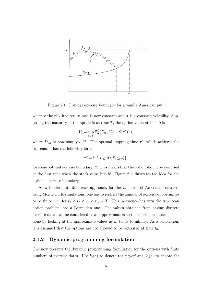
Figure 2.1: Optimal exercise boundary for a vanilla American put.
where r the risk-free return rate is now constant and σ is a constant volatility. Sup-
posing the maturity of the option is at time T , the option value at time 0 is
V0 = supτ∈T
EQ0 (D0,τ (K − S(τ))+),
where D0,τ is now simply e−rτ . The optimal stopping time τ ∗, which achieves the
supremum, has the following form
τ ∗ = inf{t ≥ 0 : St ≤ b∗t},
for some optimal exercise boundary b∗. This means that the option should be exercised
at the first time when the stock value hits b∗t . Figure 2.1 illustrates the idea for the
option’s exercise boundary.
As with the finite difference approach, for the valuation of American contracts
using Monte Carlo simulations, one has to restrict the number of exercise opportunites
to be finite, i.e. for t1 < t2 < ... < tm = T . This in essence has turn the American
option problem into a Bermudan one. The values obtained from having discrete
exercise dates can be considered as an approximation to the continuous case. This is
done by looking at the approximate values as m tends to infinity. As a convention,
it is assumed that the options are not allowed to be exercised at time t0.
2.1.2 Dynamic programming formulation
One now presents the dynamic programming formulation for the options with finite
numbers of exercise dates. Use hi(s) to denote the payoff and Vi(s) to denote the
6

value of the option at time ti with the asset price Si = s. As discussed above, Vi(s)
is defined with the assumption that the option was not exercised before time ti. To
determine the value V0(S0), a backward recursion is employed as follows:
Vm(s) = hm(s) (2.4)
Vi−1(s) = max{hi−1(s),E(Di−1,iVi(Si)|Si−1 = s)}, (2.5)
i = 1, ..., m.
As the expectation is always taken under the unique risk-neutral probability measure,
one has dropped the superscriptQ from EQ(·) for convenience. It is stated in (2.4) that
the option value at maturity is just the payoff price at that time, since there are no
more opportunities for exercising. Equation (2.5) implies that the value at exercise
time ti−1 is the maximum value between the immediate payoff and the discounted
conditional expectation of the option price at the i-th exercise time.
As this project will focus on the valuation of V0(S0), one could suppress the explicit
discounting by introducing hi(s) and Vi(s). They are defined as
hi(s) = D0,i(s)hi(s), i = 1, ..., m, (2.6)
and
Vi(s) = D0,i(s)Vi(s), i = 0, 1, ..., m. (2.7)
Whereas the Vi represents the value of the option in time-ti units of currency, Vi
expresses the value in time-t0 units. From the definitions in (2.6) and (2.7) it can be
concluded that
Vm(s) = hm(s)
and
Vi−1 = D0,i−1Vi−1(s)
= D0,i−1 max{hi−1(s),E(Di−1,iVi(Si)|Si−1 = s)}= max{hi−1(s),E(D0,i−1Di−1,iVi(Si)|Si−1 = s)}= max{hi−1(s),E(Vi(Si)|Si−1 = s)}.
7

These results transform the recursion formulation of (2.4) and (2.5) into a simplified
one:
Vm(s) =hm(s) (2.8)
Vi−1(s) = max{hi−1(s),E(Vi(Si)|Si−1 = s)}. (2.9)
i = 1, 2, ..., m
As one is prevented from exercising at time t0, at i = 1 equation (2.9) is actually
V0(S0) = E(Vi(Si)|S0),
which is the value of the option at the start of the contract. For the rest of the
dissertation, all the valuation will be done in time-t0 units.
Continuation values are crucial in the valuation of American contracts. In time-t0
units of current, the continuation value Ci at state s and time ti is defined as
Ci(s) = E(Vi+1(Si+1)|Si = s), (2.10)
for i = 0, .., m − 1. This is the value with which hi(s) compares against in (2.9).
Therefore the continuation value is the value of keeping the option alive rather than
exercising it. The key challenge faced by Monte Carlo approach in valuing American
option, is the estimation of the continuation value. With this in mind, one now
presents low-biased algorithms which use the idea of regression to estimate Ci.
2.2 Low-biased estimators
The regression-based approach assumes that Ci(s) in (2.10) can be represented as
a linear combination of basis functions from a countable Fti−1-measurable set. This
assumption is formally justified in [4] where the conditional expectation in (2.10) is
an element of the L2 space of square-integrable functions. In practice, the method
suggests that with a set of simulated Markov chain sample paths, each continuation
value Ci(s) can be approximated by a linear combination of known functions of the
current state. Typically least-square regression is used to estimate the best possible
coefficients for the approximation.
8

Suppose that the continuation valuations can be represented by a finite set of
basis functions. Then conditional expectation in (2.10) can be written as
E(Vi+1(Si+1)|Si = s) =M∑
r=1
βirψr(s), (2.11)
for some basis function ψr : <d 7→ < and constants βir, r = 1, ..., M . This is then
equivalent to
Ci(s) = βᵀi ψ(s),
where
βᵀi = (βi1, ..., βiM), ψ(s) = (ψ1(s), ..., ψM(s))ᵀ.
If one assumes that there exists a relation in the form of (2.11), then the vector
βi is given by
βi = (E(ψ(Si)ψ(Si)ᵀ))−1E(ψ(Si)Vi+1(Si+1)) ≡ B−1
ψ BψV . (2.12)
In (2.12), Bψ is an M ×M matrix, which is assumed to be nonsingular, and BψV is
a vector of length M . In side the expectation of (2.12), the variables (Si, Si+1) have
the joint distribution of the state of the underlying Markov chain at time ti and ti+1.
The coefficients βir are estimated through observing the pairs (Sij, Vi+1(Si+1,j)), j =
1, ..., b, each consisting of the state at time ti and the corresponding option value at
time ti+1. Suppose that there are independent paths (S1j, ..., Smj), j = 1, ..., b and
that the values Vi+1(Si+1) are known. Then the least-square estimate of βi through
regression is in the form of
βi = B−1ψ BψV ,
where Bψ and BψV are the sample equivalents of Bψ and BψV . This means that Bψ
is a M ×M matrix with qr entry
1
b
b∑j=1
ψq(Sij)ψr(Sij)
and BψV is a size M vector with rth entry
1
b
b∑
k=1
ψq(Sik)Vi+1(Si+1,k).
9

Function values Vi+1 at pairs of consecutive nodes (Sij, Si+1,j), j = 1, ..., b are used
to calculate Bψ and BψV . This is not possible in practice as Vi+1,j is unknown at time
ti+1. Therefore its estimation, ˆVi+1, has to be derived from the simulated paths. For
this, Tsitsiklis and Van Roy in [12, 13] suggests choosing the maximum between the
immediate exercise value hi+1 and the estimated continuation value ˆCi+1. This form
of estimation follows from the original dynamic programming problem in (2.9). In
[9] Longstaff and Schwartz however suggests a different method, which is shown later
shortly. Once the βi is obtained, it can then be used to define
ˆCi(s) = βᵀi ψ(s), (2.13)
the estimate of the continuation value at an arbitrary point s in the state space <d.
Once the continuation values have been estimated, the backward recursion from the
dynamic programming in (2.8,2.9) can be started to estimate the price at time t0.
2.2.1 Longstaff-Schwartz algorithm
With the technique of estimating continuation values through regression discussed,
one can now present the Longstaff-Schwartz algorithm.
1. Start by simulating b independent sample paths {S1j, ..., Smj}, j = 1, ..., b of
Markov chain
2. At the final state, assign each ˆVmj = hm(Smj), j = 1, ..., b.
3. Apply the following backward recursion: for i = m− 1, ..., 1,
• evaluate βi = B−1ψ BψV with the estimated values ˆVi+1,j, j = 1, ..., b by
least-square regression;
• estimate the function value as
ˆVij =
{hi(Sij), hi(Sij ≥ ˆCi(Sij);ˆVi+1,j hi(Sij < ˆCi(Sij).
(2.14)
where ˆCi is valued in the same way as (2.13).
4. Finally let ˆV0 = ( ˆV11 + ... + ˆV1b)/b.
10

The convergence of Longstaff-Schwartz method, as b →∞, was proved by Clement,
Lamberton and Protter in [4]. This sample estimate limit is the true price V0 if the
equality in (2.11) holds, meaning that only finite number of basis functions are re-
quired. If (2.11) does not hold then the limit is the value under a suboptimal exercise
policy, thus it underestimates the true value V0(S0) . In practice, the latter is true and
the method of approximating function values in (2.14) leads to low-biased estimates.
The choice for the the basis functions varies from polynomials to Fourier series.
In [9], the set of (weighted) Laguerre polynomials were used. They are of the form
Ln(S) = exp(−S/2)eS
n!
dn
dSn(Sne−S).
In this dissertation, one uses
Pn(Sij) =
(Sij − θj
θj
)n
, for n = 0, 1, ..., N, (2.15)
where θj = 1b
∑bj=1 Sij. This is a simple set of polynomials that is damped by the
average of the samples at each time step. The polynomials in (2.15) should suffice for
the pricing of the vanilla put.
2.2.2 Alternative low-biased estimator
It is possible to form an alternative low-biased estimators with the coefficients βi
obtained from the steps of Longstaff-Schwartz algorithm. One defines a stopping
time
τ = min{i : hi(Si) ≥ ˆCi(Si)},where ˆCi(Si) is obtained with βi through (2.13). The stopping time defines an exercise
policy. The policy states that the holder must exercise on the first time when the
immediate exercise value is as large as the estimated continuation value. This leads
to an estimator for a single path defined as
v = hτ (Sτ ),
which is the payoff from stopping at time τ . This estimator is low-biased because
no exercise policy can be better than an optimal policy. Conditioning on the mesh
generated by the sample paths, fixes the stopping rule and leads to
E(v|S1, ...,Sm) ≤ V0(S0),
11

where Si = (Si1, ..., Sip). The same inequality holds true for unconditional expecta-
tion. Broadie and Glasserman proved in [2] that under certain conditions, this low
estimator is asymptotically unbiased, meaning that E(v) → V0(S0) as b →∞.
This alternative low estimator can be implemented in the following algorithm:
1. First, simulate a new set of sample paths S0j, S1j, ..., Smj, j = 1, ..., p, of the
underlying Markov chain, independent of the paths used to calculate βi
2. Initialise vj = hm(Smj) and EFj = 0, j = 1, ..., p. EFj are flags indicating
whether the option has been exercised (indicated by 1) or not (indicated by 0)
on the j-th path.
3. Apply forward recursion: for i = 1, ..., m− 1,
• check if each path has 0 in their corresponding flag entry, and if
hi(Sij) ≥ ˆCi(Si), j = 1, ..., p,
where the estimate of continuation values are calculated with βi obtained
from Longstaff-Schwartz algorithm;
• for the paths with both conditions satisfied, assign hi(Sij) and 1 to their
corresponding vj and EFj.
4. The final estimate is the mean of v1, ..., vp.
2.3 High-biased estimator
So far in this chapter, two different low-biased estimators for the American options
were presented. It is also crucial to bound the true value V0(S0) from above. The rest
of the chapter will be devoted to a high-biased estimator, which is obtained through
dual formulations. The theoretical work on the dual formulations, in which the price
is represented through a minimization problem, were done by Haugh and Kogan in
[8] and Rogers in [10].
12

2.3.1 Dual problem
The dynamic programming recursion in (2.9) leads to the result that
Vi(Si) ≥ E(Vi+1(Si+1)|Si), (2.16)
for all i = 0, 1, ..., m − 1. The inequality in (2.16) is the main characteristic of a
supermartingale. Recursion (2.9) also implies that Vi(Si) ≥ hi(Si) for all i. In fact,
the process Vi(Si), i = 0, 1, ...,m, is the smallest supermartingale dominating hi(Si).
This characterisation is extended in [8] to formulate the pricing of American options
as a minimisation problem.
A continuous-time duality result is proved in [10] but a discrete-time version of
this presented here. Suppose M = {Mi, i = 0, ..., m} is a martingale with M0 = 0.
The optional stopping property of martingales states that, for any stopping time τ
with values in {1, ..., m},E(Mτ ) = M0 = 0,
which implies that
E(hτ (Sτ )) = E(hτ (Sτ )−Mτ ) ≤ E( maxk=1,...,m
(hk(Sk)−Mk)).
This leads to
E(hτ (Sτ )) ≤ infME( max
k=1,...,m(hk(Sk)−Mk)), (2.17)
where the infimum is taken over all possible martingales with initial value 0. As the
inequality in (2.17) is true for all τ , it is also true with the supremum over τ . It can
then be concluded that
supτE(hτ (Sτ )) ≤ inf
ME( max
k=1,...,m(hk(Sk)−Mk)).
With V0(S0) = supτ E(hτ (Sτ )), one arrives at the dual problem
V0(S0) ≤ infME( max
k=1,...,m(hk(Sk)−Mk)). (2.18)
One now proceeds to show that the inequality in (2.18) can be replaced with
equality. This is done by constructing a martingale M , that satisfies the required
equality relationship. Define
∆i = Vi(Si)− E(Vi(Si)|Si−1), for i = 1, ..., m, (2.19)
13

and also let
Mi = ∆1 + · · ·+ ∆i, for i = 1, ..., m, (2.20)
with M0 = 0. To prove that the process Mi is a martingale, firstly observe that
E(∆i|Si−1) = E(Vi(Si)− E(Vi(Si)|Si−1))
= E(Vi(Si)|Si−1)− E(Vi(Si)|Si−1)
= 0 (2.21)
for all i = 1, ..., m. This then leads to conclusion that
E(Mi|Si−1) = E(∆1 + · · ·+ ∆i|Si−1)
= ∆1 + · · ·+ ∆i−1 + E(∆i|Si−1)
= Mi−1
for all i = 1, ..., m. Hence Mi is a martingale.
The following uses an induction argument to show that
Vi(Si) = max{hi(Si), hi+1(Si+1)−∆i+1, ...,
h(Sm)−∆m − · · · −∆i+1}, (2.22)
for all i = 1, ..., m. This is true for i = m as Vm(Sm) = hm(Sm). Suppose (2.22) is
true at i, then by using (2.9) and (2.19) it is realised that
Vi−1(Si−1) = max{hi−1(Si−1),E(Vi(Si)|Si−1)}= max{hi−1(Si−1), Vi(Si)−∆i}= max{hi−1(Si−1), hi(Si)−∆i, ..., h(Sm)−∆m − · · · −∆i}.
This leads to the conclusion that (2.22) is true at i − 1. Thus, using Mathematical
induction, the result in (2.22) holds for all i.
The price of the option at time 0 is in the form of
V0(S0) = E(V1(S1)|S0) = V1(S1)−∆1.
Finally, by substituting V1(S1) in the above equation with (2.22), it is deduced that
V0(S0) = maxk=1,...,m
(hk(Sk)−Mk). (2.23)
14
This result verifies that equality holds in (2.18) and that the minimisation is achieved
using the martingale set out in (2.19) and (2.20).
The challenge now is to find a martingale M which is close to the optimal mar-
tingale M , so that
maxk=1,...,m
(hk(Sk)− Mk) (2.24)
can be used to calculate a high-biased estimator for the American option price.
2.3.2 Martingales for the high estimate algorithm
There are different ways to construct the martingales in (2.24), this project however
focuses on the approach that uses the approximate value functions. The approximate
value function is ˆVi(s) = max{hi(s),ˆCi(s)}. The coefficients βi obtained through
Longstaff-Schwartz algorithm are used again here to calculate ˆCi’s, the estimates of
the continuation values.
To evaluate the martingales along a simulated path S0, S1, ..., Sm, one needs the
martingale differences in (2.19). From an approximate value function, this is done by
evaluating
∆i = ˆVi(Si)− E( ˆVi(Si)|Si−1). (2.25)
The approximate value function on the right hand side can be evaluated through the
simulated path of Markov chain. The conditional expectation term however, requires
a nested simulation on the sample path from before. This is done by generating
n successors S(1)i , ..., S
(n)i , from each step Si−1 of the path. Thus, the estimate for
the conditional expectation of Vi(Si) given Si−1 is the average of those successors,
1n
∑nl=1
ˆVi(S(l)i ). This then implies that the martingale differences are
∆i = ˆVi(Si)− 1
n
n∑
l=1
ˆVi(S(l)i ), (2.26)
for all i = 1, ...,m. It is easy to check that these estimates are indeed the differences
of the required martingales. This requires verifying that they satisfy the conditionally
15

unbiased property in (2.21). Taking the conditional expectation of (2.26) leads to
E(∆i|Si−1) = E( ˆVi(Si)− 1
n
n∑
l=1
( ˆVi(S(l)i )|Si−1)
= E( ˆVi(Si)|Si−1)− 1
n
n∑
l=1
E( ˆVi(S(l)i )|Si−1)
= 0.
Using the ∆i from (2.26), an estimator for the American option can be found through
(2.24). This estimator is high-biased follows trivially from the inequality in (2.17).
The algorithm for producing the high-biased estimate has the following steps:
1. Simulate q independent paths {S1j, ..., Smj}, j = 1, ..., q of the Markov chain.
2. Set M0j = 0 and U0j = 0 for all j.
3. Start a forward recursion: for i = 1, ..., m− 1
• for each of the Si−1,j, simulate n successors S(l)i,j , l = 1, ..., n;
• calculate the martingale differences ∆ij using (2.26), noting that all theˆCi are generated using the coefficients βi from the Longstaff-Schwartz al-
gorithm;
• update so that Mij = Mi−1,j + ∆ij for all j, then set
Uij = max(Ui−1,j, hij(Sij)− Mij).
4. For the final step assign Umj = max(Um−1,j, hij(Sij)). The final estimate is the
average of the Umj for j = 1, ..., q.
This concludes the theories behind the three different algorithms that are used to
price American options. For the next chapter, the algorithms are put into practice
to produce some results for assessing their performance.
16
Chapter 3
Implementation and numericalresults
This chapter presents the results obtained from implementing the algorithms of the
three estimators described by the previous chapter. The computational codes for
these algorithms are found in the appendix section of this project. There are compar-
isons made for these estimates with estimates produced by a method from the finite
difference approach.
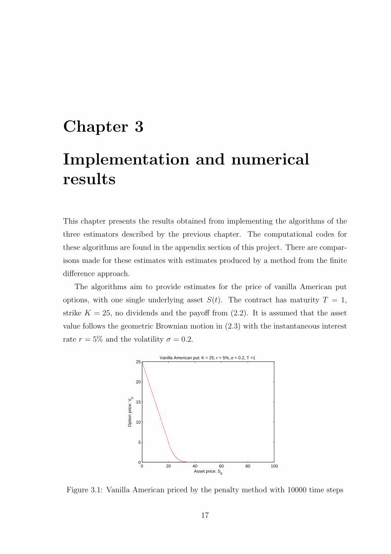
The algorithms aim to provide estimates for the price of vanilla American put
options, with one single underlying asset S(t). The contract has maturity T = 1,
strike K = 25, no dividends and the payoff from (2.2). It is assumed that the asset
value follows the geometric Brownian motion in (2.3) with the instantaneous interest
rate r = 5% and the volatility σ = 0.2.
0 20 40 60 80 1000
5
10
15
20
25Vanilla American put: K = 25, r = 5%, σ = 0.2, T =1
Asset price: S0
Opt
ion
pric
e: V
0
Figure 3.1: Vanilla American priced by the penalty method with 10000 time steps
17
For the finite difference estimates, one uses the Crank-Nicholson scheme with the
penalty method. The idea of this method is to ’penalise’ if the inequality in (1.1) is
violated, by solving
Lu = ρ max(g − u, 0)
with a positive penalty parameter ρ. More details on this method is presented in
Chapter 28 of [5]. Figure 3.1 is a graph showing the estimates for the American puts
calculated with penalty method and 10000 time steps. The error tolerant level for
this method is set at 10−8, which implies that the produced estimates give a very
good representation of the true values. The curve in Figure 3.1 is shown here to get
an overview of the option prices with a range of initial stock values.
3.1 Low-biased estimates
This section presents some numerical results for the low-biased estimates. As the
option is path-dependent, the asset values at each of the exercise times need to be
simulated for all sample paths. For this, Euler-Maruyama method is used to approx-
imate the stochastic differential equation in (2.3). Hence for all i, with a given Si,
the asset estimate for the next time step is produced by the discretisation:
Si+1 = Si(1 + rh + σ√
hZi), (3.1)
where h is the size of the interval between two consecutive exercise times, and Zi is a
normally distributed random variable with mean 0 and variance 1. Samples of Zi are
obtained through Marsaglia’s ziggurat algorithm, a random number generator. For
the implementation of Longstaff-Schwartz algorithm, one has discretised the duration
of the option into 100 equal sized exercise times. The number of sample paths taken
for the Monte Carlo simulation are 10000. The basis functions, used for the least-
square regressions applied along the paths, are the first 4 terms of the polynomials
stated in (2.15). Thus, the continuation values, Ci, are estimated by
ˆCi(s) =4∑
n=0
βᵀi
(Sij − θj
θj
)n
.
As well as estimating the value of the option at time t0, a record of the coefficients ˆbetai
for all i = 1, ..., m − 1 estimated through regression is also kept in memory for later
18
uses in the other algorithms. The alternative low-biased estimates are generated with
a second set of 10000 sample paths, independent of the paths used for the Longstaff-
Schwartz estimates. The βi obtained from the regressions are used to calculate the
approximated continuation values at each of the 100 exercise times.
3.1.1 Some analysis on the results
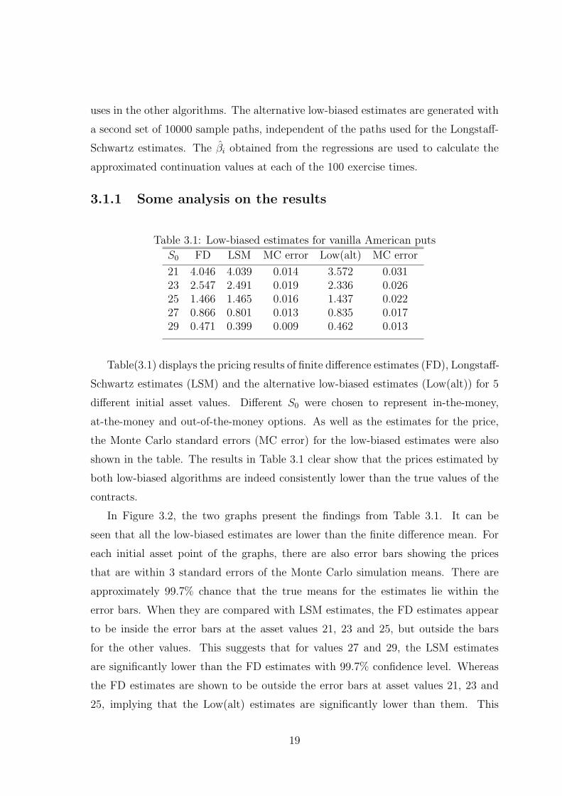
Table 3.1: Low-biased estimates for vanilla American puts
S0 FD LSM MC error Low(alt) MC error
21 4.046 4.039 0.014 3.572 0.03123 2.547 2.491 0.019 2.336 0.02625 1.466 1.465 0.016 1.437 0.02227 0.866 0.801 0.013 0.835 0.01729 0.471 0.399 0.009 0.462 0.013
Table(3.1) displays the pricing results of finite difference estimates (FD), Longstaff-
Schwartz estimates (LSM) and the alternative low-biased estimates (Low(alt)) for 5
different initial asset values. Different S0 were chosen to represent in-the-money,
at-the-money and out-of-the-money options. As well as the estimates for the price,
the Monte Carlo standard errors (MC error) for the low-biased estimates were also
shown in the table. The results in Table 3.1 clear show that the prices estimated by
both low-biased algorithms are indeed consistently lower than the true values of the
contracts.
In Figure 3.2, the two graphs present the findings from Table 3.1. It can be
seen that all the low-biased estimates are lower than the finite difference mean. For
each initial asset point of the graphs, there are also error bars showing the prices
that are within 3 standard errors of the Monte Carlo simulation means. There are
approximately 99.7% chance that the true means for the estimates lie within the
error bars. When they are compared with LSM estimates, the FD estimates appear
to be inside the error bars at the asset values 21, 23 and 25, but outside the bars
for the other values. This suggests that for values 27 and 29, the LSM estimates
are significantly lower than the FD estimates with 99.7% confidence level. Whereas
the FD estimates are shown to be outside the error bars at asset values 21, 23 and
25, implying that the Low(alt) estimates are significantly lower than them. This
19

observation may suggest that the Longstaff-Schwartz algorithm is best used for pricing
out-of-the-money contracts, whereas the alternative low-biased for pricing in-the-
money contracts.
22 24 26 28
0.5
1
1.5
2
2.5
3
3.5
4
Compare FD and LSM
S0
V0
FDLSM
22 24 26 28
0.5
1
1.5
2
2.5
3
3.5
4
Compare FD and Low(alt)
S0
V0
FDLow(alt)
Figure 3.2: Compare low-biased estimates with FD estimates
3.1.2 Sources of errors of the estimates
There are three different sources of errors that affect the accuracies of the low-biased
estimates. The first one is associated with the discretisation of the exercise dates,
which makes the exercise policy of the estimators suboptimal. To reduce this, more
time steps can be taken in the implementation of the algorithm. Another source
of errors comes from the least-square regression used to estimate the continuation
values, Ci. As the regression employs only finite numbers of polynomials for basis
functions, continuation values are not represented with total accuracy. One could
increase the number of basis functions to form better estimates for the continuation
values. Finally, there are also the usual errors from using finite number of sample
paths for Monte Carlo simulations. To reduce the standard errors from Monte Carlo,
a larger number of sample paths can be taken for estimation.
After listing the possible ways that the accuracy of the estimates are affected,
one would like to investigate the effects on the estimates caused by the limitations in
practice. This is done by varying the parameters and inputs that cause inaccuracies
20
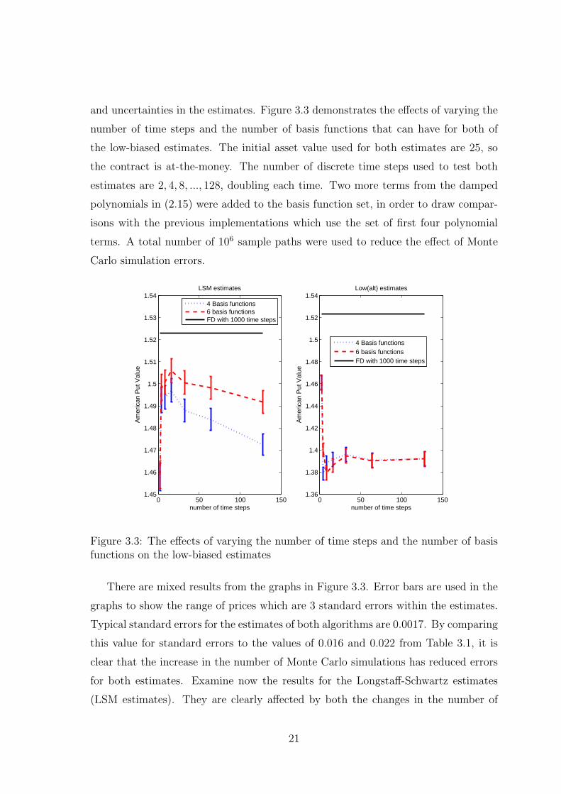
and uncertainties in the estimates. Figure 3.3 demonstrates the effects of varying the
number of time steps and the number of basis functions that can have for both of
the low-biased estimates. The initial asset value used for both estimates are 25, so
the contract is at-the-money. The number of discrete time steps used to test both
estimates are 2, 4, 8, ..., 128, doubling each time. Two more terms from the damped
polynomials in (2.15) were added to the basis function set, in order to draw compar-
isons with the previous implementations which use the set of first four polynomial
terms. A total number of 106 sample paths were used to reduce the effect of Monte
Carlo simulation errors.
0 50 100 1501.45
1.46
1.47
1.48
1.49
1.5
1.51
1.52
1.53
1.54
number of time steps
Am
eric
an P
ut V
alue
LSM estimates
4 Basis functions6 basis functionsFD with 1000 time steps
0 50 100 1501.36
1.38
1.4
1.42
1.44
1.46
1.48
1.5
1.52
1.54
number of time steps
Am
eric
an P
ut V
alue
Low(alt) estimates
4 Basis functions6 basis functionsFD with 1000 time steps
Figure 3.3: The effects of varying the number of time steps and the number of basisfunctions on the low-biased estimates
There are mixed results from the graphs in Figure 3.3. Error bars are used in the
graphs to show the range of prices which are 3 standard errors within the estimates.
Typical standard errors for the estimates of both algorithms are 0.0017. By comparing
this value for standard errors to the values of 0.016 and 0.022 from Table 3.1, it is
clear that the increase in the number of Monte Carlo simulations has reduced errors
for both estimates. Examine now the results for the Longstaff-Schwartz estimates
(LSM estimates). They are clearly affected by both the changes in the number of
21

basis functions and the number of time steps. It appears that the estimates with
the higher number of basis functions consistently outperform the one with less basis
functions. This observation is most clear for time steps 25, 26 and 27, since there
are no overlappings for the error bars in these time steps. Within the same set of
basis functions, the estimates are affected by the number of time steps. This is most
significant at very low number of time steps, with a large increase between using 2
and 4 as the numbers of times steps. Before they drop lower at 27 time steps, the
estimates were quite consistent between 25 and 26, demonstrated by having a clear
overlapping for their error bars. The decrease in the value of the estimates at 27 is
most significant for the implementation using only four basis functions. Its estimate
at 27 is more than 3 standard errors away from the estimate at 26. This may indicate
that there are no complete independency between the errors caused by the number
of basis functions and by the number of discrete exercise dates. The results from
alternative low-biased estimates (Low(alt) estimates) are quite different to the ones
from LSM estimates. There are almost no indications of difference between two sets
of estimates using different number of basis functions, especially for 25, 26 and 27
numbers of time steps. This is shown by the consistent overlappings of their error
bars. There are also less variations caused by changing the number of exercise dates,
apart from the results with really low numbers. This suggests that the alternative
low-biased estimates are less likely to be affected by changes made in the number of
basis functions and in the number of exercise dates. Whereas the opposite seems to
be true for LSM estimates.
3.2 High-biased estimate
This section presents results obtained through implementing the high-biased estimate
algorithm. It also shows the effects on the estimates when antithetic variables are
used in the algorithm with the view of reducing possible errors.
3.2.1 Results for two different numbers of sub-paths
The parameters used in the implementation are the same as the low-biased estimates.
The number of discrete time steps used for all the high-biased estimates is 100. The
number of Monte Carlo simulations used is 1000. One chooses 10 and 100 as the
22
numbers of sub-paths used for estimating ∆i from (2.26). This is done so that the
effects of changing in the number of sub-paths can be observed. These results are
then recorded in Table 2.24.
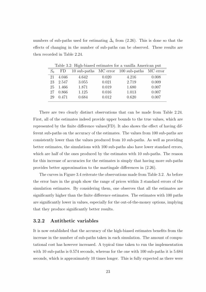
Table 3.2: High-biased estimates for a vanilla American put
S0 FD 10 sub-paths MC error 100 sub-paths MC error
21 4.046 4.642 0.020 4.216 0.00823 2.547 3.055 0.021 2.719 0.00925 1.466 1.871 0.019 1.680 0.00727 0.866 1.125 0.016 1.013 0.00729 0.471 0.684 0.012 0.620 0.007
There are two clearly distinct observations that can be made from Table 2.24.
First, all of the estimates indeed provide upper bounds to the true values, which are
represented by the finite difference values(FD). It also shows the effect of having dif-
ferent sub-paths on the accuracy of the estimates. The values from 100 sub-paths are
consistently lower than the values produced from 10 sub-paths. As well as providing
better estimates, the simulations with 100 sub-paths also have lower standard errors,
which are half of the ones produced by the estimates with 10 sub-paths. The reason
for this increase of accuracies for the estimates is simply that having more sub-paths
provides better approximation to the martingale differences in (2.26).
The curves in Figure 3.4 reiterate the observations made from Table 3.2. As before
the error bars in the graph show the range of prices within 3 standard errors of the
simulation estimates. By considering them, one observes that all the estimates are
significantly higher than the finite difference estimates. The estimates with 100 paths
are significantly lower in values, especially for the out-of-the-money options, implying
that they produce significantly better results.
3.2.2 Antithetic variables
It is now established that the accuracy of the high-biased estimates benefits from the
increase in the number of sub-paths taken in each simulation. The amount of compu-
tational cost has however increased. A typical time taken to run the implementation
with 10 sub-paths is 0.574 seconds, whereas for the one with 100 sub-paths it is 5.684
seconds, which is approximately 10 times longer. This is fully expected as there were
23

21 22 23 24 25 26 27 28 290.5
1
1.5
2
2.5
3
3.5
4
4.5
High−biased estimates for American put options
S0
V0
FD100 sub−paths10 sub−paths
Figure 3.4: High-biased estimates for American puts using different numbers of sub-paths
10 times more simulations done at each step of the calculations. It is possible to
apply variance reduction techniques to provide better estimates without increasing
the number of sub-paths. One of those techniques involves introducing antithetic
variables into the algorithm.
As the successors in the sub-paths of high-biased algorithm can also be generated
by the Euler-Maruyama method in (3.1), one can estimate the approximate values in
the second term on the right hand side of (2.25) with
ˆVi(S(l)i ) ≈ ˆVi(Si−1(1 + rh)) +
∂ ˆV
∂sσ√
hSi−1Z(l)i . (3.2)
This implies that the variability of ˆVi comes from the stochastic term. Antithetic
variables can be used to reduce (3.2) to the leading order term, as the value is ap-
proximately linear. This means that for every sub-path, as a sample of random
variable Z(l) is generated, −Z(l) is introduced as another sample. Chapter 4 of [6]
provides more details on the antithetic variates technique.
In Table 3.3, the estimates produced by using standard algorithm with 100 sub-
paths (Std(100)) are compared with the estimates provided by adding antithetic vari-
ables into the algorithm and using only 10 sub-paths (AntiVar(10)). The last column
of Table 3.3 shows the ranges that are within 3 standard errors of the estimates with
24

Table 3.3: Applying antithetic variates to the high-biased estimates of American puts
S0 Std(100) MC error AntiVar(10) MC error 3 MC errors range
21 4.216 0.008 4.120 0.007 (4.101, 4.140)23 2.719 0.009 2.663 0.007 (2.644, 2.682)25 1.680 0.007 1.647 0.006 (1.631, 1.664)27 1.013 0.007 0.994 0.005 (0.978, 1.011)29 0.620 0.007 0.611 0.006 (0.594, 0.629)
antithetic variables. There are two very clear improvements made by introducing the
antithetic variables into the high-biased algorithm. The first observation is that the
standard errors for both implementations of the algorithm is practically the same.
A typical computing time for producing estimates with antithetic variables is 1.123
seconds, about a fifth of the time required for the estimates of Std(100) algorithm.
The time is only about twice the one required for the estimates with 10 sub-paths
but without antithetic variables. This demonstrates that, by having antithetic vari-
ables there are indeed reductions made to variance in the form of standard errors. It
can be seen that almost all of the estimates from Std(100) algorithm are higher than
and outside of the corresponding ranges provided by AntiVar(10) algorithm. This
is significantly enough to suggest that the latter algorithm produces lower estimates
than the former. This means that the AntiVar(10) estimates are closer to the true
values than the Std(100) estimates. With the two observations from above, one con-
cludes that including antithetic variables in the high-biased algorithm leads to better
estimates for the true price of American puts.
This then concludes the current chapter on the numerical results obtained through
the implementation of the three different algorithms. The next and final chapter will
be a summary of the dissertation and provides some closing remarks on the topic of
pricing American options using Monte Carlo simulations.
25

Chapter 4
Summary and concludingcomments
In this dissertation, three different pricing algorithms of American option contacts
using Monte Carlo simulation were investigated. The pricing of the American style
options using simulation, aims to solve discretised dynamically programming prob-
lem. This leads to the approximation of the continuation values for each discrete
exercise date. All of the algorithms presented here use regression techniques, i.e.
the least-square regression, to estimate the continuation values. Longstaff-Schwartz
algorithm first simulates one single single set of stock sample paths. By stepping
back in time it then applies the regression to estimate the continuation values, de-
riving approximate values to the price at time zero in the process. The alternative
low-biased algorithm uses the regression results from Longstaff-Schwartz algorithm
and an sub-optimal exercise policy, to price the option with an independent set of
sample paths. The theory developed on dual problems shows that the valuation of
the option is a maximisation problem involving a certain class of martingales. The
high-biased algorithm looks to estimate the conditional expectations in the differences
of these martingales using sub-paths in its simulation. The regression results from
Longstaff-Schwartz algorithm are again used in this final algorithm.
The three algorithms were then implemented to price vanilla American puts, so
that numerical results were produced for analysis. Values obtained from a finite dif-
ference scheme were used as reference to represent the true prices of these contracts.
A simple set of damped polynomials were chosen as the basis functions used for
regression. The results showed that both Long-Schwartz and the alternative biased-
26
low algorithms produced estimates that were consistently lower than the true price.
There were also observations that the Longstaff-Schwartz algorithm produced closer
estimates for out-of-the-money contracts, whereas the alternative low-biased algo-
rithm were better for in-the-money contracts. It is then suggested that the accuracy
of the estimates is affected by three different sources of errors. They are from the
discretisation of the exercise dates, the estimation of continuation values with finite
number of basis functions and the finiteness of the Monte Carlo simulations. The ef-
fects of alterations in these areas on the estimates were examined. It was shown that
standard errors were reduced by having more Monte Carlo simulations. There were
significantly indications that the estimates from Longstaff-Schwartz algorithm varied
for having different numbers of time steps and different numbers of basis functions.
This is however not the case for the alternative low-biased estimates as they do not
show any significant variations. The results from high-biased algorithm confirmed
that the estimates are consistently higher than the true values. The effects of differ-
ent numbers of sub-paths were evident, such that having more sub-paths increased
the accuracy of the results but in the expense of spending more computational time.
This then leads to an investigation on introducing antithetic variables into the algo-
rithm. The resulting table shows that the estimates using 10 sub-paths and antithetic
variables were as accurate as, if not better than, the estimates produced by only using
100 sub-paths. The computing cost for the former estimates were a fifth of the latter
estimates.
There are few possible improvements and extensions that can be made for this
dissertation. One of which is to apply these algorithms to more exotic American
options, especially the contracts with high dimensions. As it was discussed in the
introduction, the finite difference approach works very well for options at low dimen-
sions but suffers from the “curse of dimensionality” for high dimensions. It would be
of great interest to investigate whether in practice the algorithms provide effective
lower and upper bounds with less computational time in comparison to finite differ-
ence methods. Another area that could be looked at is how to utilise these algorithms
in deriving Greeks of the contracts. The Longstaff-Schwartz algorithm’s estimate to
the values at each time step is discontinuous, which would be a problem for using
the path-wise sensitivity method for the Greeks. Effects of applying other variance
27

reduction techniques to the high-biased estimates could also be looked at. One such
technique extends the idea of (3.2) further. By taking the expectation of ˆVi(Si) given
Si−1, one concludes that
E( ˆVi(Si)|Si−1) ≈ ˆVi−1(Si−1(1 + h)),
which leads to the realisation that
ˆVi(Si)− E( ˆVi(Si)|Si−1) ≈ ∂ ˜Vi
∂sσ√
hSi−1Zi.
This suggests that one could look to estimate the martingale differences in (2.26) with
∆i =∂ ˆVi
∂sσ√
hSi−1Zi,
where ∂ ˆVi
∂scan be calculated by simply differentiating the estimated continuation val-
ues. As the continuation values are approximated using polynomials, the estimates
of the partial derivatives can be easily calculated. Valuing ∆i this way requires less
computing time than the original high-biased algorithm as well as the one with anti-
thetic variables. This is essentially because there are no sub-paths required for this
approach. It would be interesting to see whether this works in practice and how it
compares to the existing results from this dissertation.
28
Appendix A
Appendix
A.1 The implementation of Longstaff-Schwartz al-
gorithm
% Pricing American Put using Longstaff-Schwartz method
% Stock underlying dynamics: dS = r*S dt + sig*S dW
clear all; close all
randn(’state’,0)
format long
savefile = ’Beta_2.mat’;
tic;
r = 0.05;
sig = 0.2;
T = 1;
S0 = 23;
K = 25;
N = 100;
M = 1e+4;
Beta_save = cell(2,1);
29

sum1 = zeros(2,1);
sum2 = sum1;
h = T/N;
% Discount value for each time step:
Disc = exp(-r*h);
% Recording betas
beta = zeros(4,N-1);
beta1 = zeros(6,N-1);
%
% Simulate M independent paths first,
% for regression.
%
S = ones(M, N+1);
S(:,1) = S0*ones(M,1);
for n = 1:N
dW = sqrt(h)*randn(M,1);
S(:,n+1) = S(:,n).*(1+r*h+sig*dW);
end
%
% Discount all values to become time-0 units
%
DiscAll = cumprod(Disc*ones(M,N),2);
CE = DiscAll.*max(K-S(:,2:end),0);
V1 = CE(:,end);
V2 = V1;
30

%
% Working backwards to evaluate continuation values
% and then Max(payoff, continuation).
%
for q = (N:-1:2)
A = S(:,q);
eA = mean(A);
% L-S recommends taking only in-the-money nodes
% index = logical(max(K-A,0));
index = true(M,1);
X = A(index);
Y1 = V1(index);
Y2 = V2(index);
eX = mean(X);
% First set has (1, S, S^2, S^3):
regression_matrix_1 = [ones(size(X,1),1),(X-eX)/eX,((X-eX)/eX).^2,...
((X-eX)/eX).^3];
% Second has (1, S, S^2, ... , S^5):
regression_matrix_2 = [ones(size(X,1),1),(X-eX)/eX,((X-eX)/eX).^2,...
((X-eX)/eX).^3,((X-eX)/eX).^4,((X-eX)/eX).^5];
%Regression are done by finding the beta’s.
beta(:,q-1) = regression_matrix_1\Y1;
beta1(:,q-1) = regression_matrix_2\Y2;
% Estimated continuation values:
CC1 = [ones(size(A,1),1) (A-eA)/eA ((A-eA)/eA).^2 ((A-eA)/eA).^3]...
*beta(:,q-1);
31

CC2 = [ones(size(A,1),1) (A-eA)/eA ((A-eA)/eA).^2 ...
((A-eA)/eA).^3 ((A-eA)/eA).^4 ((A-eA)/eA).^5]*beta1(:,q-1);
% Comparing exercise values and continuation values
index1 = (CE(:,q-1)>=CC1);
index2 = (CE(:,q-1)>=CC2);
% Longstaff-Schwartz method:
V1(~index1) = V1(~index1);
V2(~index2) = V2(~index2);
% % Tsitsiklis and Van Roy:
% V1(~index1)= CC1(CE(index,q-1)<CC1);
% V2(~index2)= CC2(CE(index,q-1)<CC2);
V1(index1)= CE(index1,q-1);
V2(index2)= CE(index2,q-1);
end
sum1(1) = sum(V1);
sum1(2) = sum(V2);
sum2(1) = sum((V1).^2);
sum2(2) = sum((V1).^2);
VLS = sum1/M
sd = sqrt((sum2/M-VLS.^2)/M)
Beta_save{1} = beta;
Beta_save{2} = beta1;
% Saving the state of the generator
32

rstate = randn(’state’);
toc
% Save results for betas in file for Low and High-biase valuation.
save(savefile, ’Beta_save’,’S0’,’r’,’K’,’T’,’sig’,’rstate’,’N’);
A.2 The implementation for the alternative low-
biased algorithm
%Alternative Low-biased Estimates
clear all; close all
format long
% load Betas got from regression.
load(’Beta_2.mat’)
randn(’state’,rstate)
tic;
M = 1e+4;
h = T/N;
% Discount value for each time step:
Disc = exp(-r*h);
% load betas from regression done with LSM
beta = Beta_save{1};
beta1 = Beta_save{2};
sum1 = zeros(2,1);
sum2 = zeros(2,1);
33

for m = 1:1
S = ones(M, N+1);
S(:,1) = S0;
% Simulate Markov chain paths
for n = 1:N
dW = sqrt(h)*randn(M,1);
S(:,n+1) = S(:,n).*(1+r*h+sig*dW);
end
CE = max(K-S(:,end),0);
% Set inital value to the discounted payoff at terminal.
VLow1 = Disc^N*CE;
VLow2 = Disc^N*CE;
% Set flags initially to be 0.
index1 = true(M,1);
index2 = index1;
for n = 1:N-1
X = S(:,n+1);
e = mean(X);
CE = Disc^n*max(K-X,0);
% Calculating continuation values
CC1 = [ones(size(X,1),1) (X-e)/e ((X-e)/e).^2 ((X-e)/e).^3]...
*beta(:,n);
CC2 = [ones(size(X,1),1) (X-e)/e ((X-e)/e).^2 ((X-e)/e).^3 ...
((X-e)/e).^4 ((X-e)/e).^5]*beta1(:,n);
34

% Check if the ’yet-to-be’ exercised paths have
% its immediate exercise value greater than continuation values.
% Flags are updated.
index1 = ((CE.*index1)>=(CC1.*index1));
index2 = ((CE.*index2)>=(CC2.*index2));
% Update the values.
VLow1(index1) = CE(index1);
VLow2(index2) = CE(index2);
end
sum1(1) = sum1(1) + sum(VLow1);
sum1(2) = sum1(2) + sum(VLow2);
sum2(1) = sum((VLow1).^2) + sum2(1);
sum2(2) = sum((VLow2).^2) + sum2(2);
end
avrg = sum1/(m*M)
sd = sqrt((sum2/(m*M)-avrg.^2)/(m*M))
toc
A.3 The implementation of high-biased algorithm
% High-biased American Put Valuation
clear all; close all
format long
% load Betas got from regression.
35

load(’Beta_2.mat’)
randn(’state’,rstate)
tic;
M = 1000;
Mini_Path = 10;
h = T/N;
% Discount value for each time step:
Disc = exp(-r*h);
sum1 = zeros(2,1);
sum2 = zeros(2,1);
beta = Beta_save{1};
for m = 1:1
%
% Simulate M independent paths first
%
S = ones(M, N+1);
S(:,1) = S0*ones(M,1);
for n = 1:N
dW = sqrt(h)*randn(M,1);
S(:,n+1) = S(:,n).*(1+r*h+sig*dW);
end
CC_nested = zeros(M, Mini_Path);
CC_nested_Anti = CC_nested;
% Set zeros to the estimates and the martingale for both
36

% with and without antithetic varialbes
VHigh = zeros(M,1);
VHigh_Anti = VHigh;
MAccum = zeros(M,1);
MAccum_Anti = MAccum;
for n = 1:N-1
A = S(:,n+1);
A_pre = S(:,n);
e = mean(A);
CE = Disc^n*max(K-A,0);
% First term on the right hand side
V_est = max(CE, [ones(M,1) (A-e)/e ((A-e)/e).^2 ((A-e)/e).^3]...
*beta(:,n));
% Sub-paths required for estimating conditional expectation
dW = sqrt(h)*randn(M,Mini_Path);
% Successor values
A_Con = (1+r*h+sig*dW).*repmat(A_pre,1,Mini_Path);
A_Con_Anti = (1+r*h-sig*dW).*repmat(A_pre,1,Mini_Path);
e_pre = mean(A_Con);
e_pre_Anti = mean(A_Con_Anti);
for k = 1:Mini_Path
% Continuation values for the sub-paths
CC_nested(:,k) = [ones(M,1),(A_Con(:,k)-e_pre(k))/e_pre(k),...
((A_Con(:,k)-e_pre(k))/e_pre(k)).^2,...
((A_Con(:,k)-e_pre(k))/e_pre(k)).^3]*beta(:,n);
CC_nested_Anti(:,k) = [ones(M,1),(A_Con_Anti(:,k)-...
e_pre_Anti(k))/(e_pre_Anti(k)),...
(A_Con_Anti(:,k)-e_pre_Anti(k))/...
37

e_pre_Anti(k)).^2,((A_Con_Anti(:,k)...
-e_pre_Anti(k))/e_pre_Anti(k)).^3]*beta(:,n);
end
% Second term of the right hand side
V_nested = max(Disc^n*max(K-A_Con,0), CC_nested);
V_nested_Anti = max(Disc^n*max(K-A_Con_Anti,0), CC_nested_Anti);
% Update the martingales
MAccum = MAccum+(V_est-mean(V_nested,2));
MAccum_Anti = MAccum_Anti+(V_est-mean([V_nested V_nested_Anti],2));
% Update the estimates
VHigh = max(VHigh, CE-MAccum);
VHigh_Anti = max(VHigh_Anti, CE-MAccum_Anti);
end
% Final time step
CE = Disc^N*max(K-S(:,end),0);
A_pre = S(:,N);
dW = sqrt(h)*randn(M,Mini_Path);
A_Con = (1+r*h+sig*dW).*repmat(A_pre,1,Mini_Path);
A_Con_Anti = (1+r*h-sig*dW).*repmat(A_pre,1,Mini_Path);
V_nested = Disc^N*max(K-A_Con,0);
MAccum = MAccum+(CE-mean(V_nested,2));
VHigh = max(VHigh, (CE-MAccum));
V_nested_Anti = Disc^N*max(K-A_Con_Anti,0);
MAccum_Anti = MAccum_Anti+(CE-mean([V_nested V_nested_Anti],2));
VHigh_Anti = max(VHigh_Anti, (CE-MAccum_Anti));
38

sum1(1) = sum1(1) + sum(VHigh);
sum1(2) = sum1(2) + sum(VHigh_Anti);
sum2(1) = sum(VHigh.^2) + sum2(1);
sum2(2) = sum(VHigh_Anti.^2) + sum2(2);
end
avrg = sum1/(m*M)
sd = sqrt((sum2/(m*M)-avrg.^2)/(m*M))
toc
39

References
[1] P. Bossaerts. Simulation estimators of optimal early exercise, working paper,
1988.
[2] M. Broadie and P. Glasserman. A stochastic mesh method for pricing high-
dimensional american options. Journal of Compuatational Finance, 7, 2004.
[3] J Carrie. Valuation of early-excercise price of options using simulations and
nonparametric regression. Insurance: Mathematics and Economics, 19:19–30,
1996.
[4] E. Clement, D. Lamberton, and P. Protter. An analysis of the longstaff-schwartz
algorithm for american option pricing. Finance and Stochasics, 6:449–471, 2002.
[5] D.J. Duffy. Finite Difference Methods in Financial Engineering: A Partial Dif-
ferential Equation Approach. Wiley, 2006.
[6] P. Glasserman. Monte Carlo Methods in Financial Engineering. Springer, 2004.
[7] J.M. Harrison and D. Kreps. Martingales and arbitrage in multiperiod securities
markets. Journal of Economic Theory, 20:381–408, 1979.
[8] M. Haugh and L. Kogan. Pricing american options: a duality approach. Opera-
tions Research, 52:258 – 270, 2001.
[9] F.A. Longstaff and E.S. Schwartz. Valuing american options by simulation: a
simple least-squares approach. The Review of Financial Studies, 14:113–147,
2001.
[10] L.C.G. Rogers. Monte carlo valuation of american options. Mathematical Fi-
nance, 12:271–286, 2002.
40

[11] J.A. Tilley. Valuing american options in a path simulation model. Transactions
of the Society of Actuaries, 45:83–104, 1993.
[12] J. Tsitsiklis and B. Van Roy. Optiomal stopping of markov processes: Hilbert
space theory, approximation algorithms, and an application to pricing high-
dimensional financial derivatives. IEEE Transactions on Automatic Control,
44:1840–1851, 1999.
[13] J. Tsitsiklis and B. Van Roy. Regression methods for pricing complex american-
style options. IEEE Transactions on Neural Networks, 12:694–703, 2001.
41