1

Monsoon 2013 – A Report, No ESSO/IMD/Synoptic Met/01-2014/15, India Meteorological Department

Chapter 7

PERFORMANCE OF NWP MODELS FOR SHORT RANGE AND MEDIUM RANGE WEATHER FORECASTS

S.K. Roy Bhowmik, V.R. Durai, Ananda K. Das, S.D. Kotal and M. Rathee

This chapter discusses the verification of operational forecasts in the short range

(Up to 3 days) and medium range (up to 7 days) weather forecasts based on GFS and

WRF models issued for the 2013 southwest monsoon season.

5.1 Introduction

The Global Forecast System (GFS), adopted from National Centre for

Environmental Prediction (NCEP), at T382L64 (~ 35 km in horizontal) resolution was

implemented at India Meteorological Department (IMD), New Delhi on IBM based High

Power Computing Systems (HPCS) in May 2010. The upgraded version of the GFS (GSI

3.0.0 and GSM 9.1.0) model at T574L64 (~ 25 km) resolution has been also operated in

the experimental mode since 1 June 2011 and real-time outputs are made available

through the national web site of IMD (www.imd.gov.in).

The objective of this report is to document the performance skill of this model in

spatial and temporal scale during summer monsoon 2013. Rainfall is one of the most

2

difficult parameter to predict due to its large spatial and temporal variation. A detailed

rainfall prediction skill of the model is described in this report. For the comparison

purpose, performance statistics of multi-model ensemble (MME) forecasts and global

model forecasts of other centers are also included. Daily rainfall analysis generated at

the resolution of 0.5o resolution from the use of daily rain gauge observations (IMD) and

satellite (TRMM) derived quantitative precipitation estimates is used as the observed

dataset for the validation purpose.

The results showing the ability of the model to predict genesis of low pressure

system and other characteristic flow features of south west monsoon are also discussed.

GFS T574 performance statistics of upper level wind, temperature and relative humidity

forecasts over Indian monsoon regions are also described.

5.1.2 The Global Forecast System (GFS)

The Global Forecasting System (GFS) run at IMD is a primitive equation spectral

global model with state of art dynamics and physics (Kanamitsu 1989, Kalnay et al. 1990,

Kanamitsu et al. 1991; Durai and Roy Bhowmik. 2013). The GFS, adopted from National

Centre for Environmental Prediction (NCEP), at T382L64 (~ 35 km in horizontal)

resolution was implemented at India Meteorological Department (IMD), New Delhi on IBM

based High Power Computing Systems (HPCS) in May 2010. The upgraded version of the

GFS (GSI 3.0.0 and GSM 9.1.0) model at T574L64 (~ 25 km) resolution has been also

operated in the experimental mode since 1 June 2011 and real-time outputs are made

available to the national web site of IMD (www.imd.gov.in). More details about the global

model GFS are available at http://www.emc.ncep.noaa.gov/gmb/moorthi/gam.html. The

main objective of this study is to investigate the precipitation forecast skill of the GFS

T574 in the medium range time scale over Indian region during South West Monsoon

2013. Daily rainfall analysis from National data center (NDC) , IMD Pune generated at

the resolution of 0.5 degree resolution from the use of daily rain gauge observations

(IMD) and satellite (TRMM) derived quantitative precipitation estimates is used as the

observed dataset for the validation purpose.

The list of type of data being used in Global Data Assimilation System at IMD is

available at IMD web site. The Global Data Assimilation (GDAS) cycle runs 4 times a day

(00, 06, 12 and 18 UTC). The assimilation system is a global 3-dimensional variational

technique, based on NCEP Grid Point Statistical Interpolation (GSI 3.0.0) scheme, which

is the next generation of Spectral Statistical Interpolation (SSI). Forecast Integration for 7

days. The analysis and forecast for 7 days is performed using the HPCS installed in IMD

3

Delhi. One GDAS cycle and seven day forecast (168 hour) at T574L64 (~ 20 km in

horizontal) resolution takes about 1 hour 30 minutes on IBM Power 6 (P6) machine using

20 nodes with 7 tasks (7 processors) per node.

5.1.3 Verification Procedures

In this study, rainfall verifications were carried out for GFS T574 model run at 00

UTC against daily rainfall analysis at the resolution of 50 km based on the merged rainfall

data combining gridded rain gauge observations prepared by IMD Pune for the land areas

and TRMM 3B42RT data for the Sea areas (Durai et al. 2010b). In order to examine the

performance of the model in different homogeneous part of the country, we selected six

representative region (square/rectangular domain) for (a) All India (land areas: (Lon: 68oE

– 98oE, Lat: 9

oN – 37

oN), (b) Central India (CE: Lon: 75

oE – 80

oE, Lat: 19

o – 24

oN),

covering Vidarbha and neighborhoods, (c) East India (EI: Lon: 75oE – 80

oE, Lat: 19

o –

24oN), covering Orissa and neighborhoods, (d) North-east India (NE: Lon: 90

oE – 95

oE,

Lat: 24oN -29

oN), (e) North-west India (NW: Lon: 75

oE – 80

oE, Lat: 25

oN -30

oN),

covering Rajasthan and Haryana, (f) South Peninsular India (SP: Lon: 76oE - 81

oE, Lat:

12oN- 17

oN), covering Kerala and neighborhood and (g) West coast of India (WC: Lon:

70oE - 75

oE, Lat: 13

oN - 18

oN), covering Konkan-Goa. Performance for each region is

evaluated by computing grid point by point comparisons (Durai et al. 2010b; Roy

Bhowmik. et al. 2008). The temporal and spatial distribution of observed and model

predicted rainfall has been studied. Direct comparison is made of accumulated values of

seasonal mean error (bias), root mean square Error (RMSE) and correlation coefficient

(CC). These are defined as follows:

Mean error (Bias) )(1

1N

i

iiNOXBIAS

Root mean square error 2

1

1 )(

N

i

iiNOXRMSE

Anomaly Correlation coefficient:

2

1

2

1

1

)()(

))((

N

i

ii

N

i

ii

ii

N

i

ii

OOXX

COCX

ACC

Where N is the total number of samples, i = 1, 2… N and X is the GFST574

rainfall estimation, C is the observed climatology and O is the gauge observation

at the grids. In addition to these simple measures, a number of categorical

statistics are applied.

4

5.1.4 Verification Results

5.1.4.1 Rainfall Prediction Skill

5.1.4.1.1 Observed and forecast fields

Fig.5.1 illustrates the spatial distribution of mean rainfall (mm/day) of the season

based on the observations and Day-1 to Day-5 forecast from GFS T574 for the period

Fig.5.1: Spatial distribution of seasonal mean observed rainfall and Day-1, Day-3 and Day-5 forecast rainfall (mm/day) from GFS T574 for the period from 1 June to 30 September 2013

5

from 1 June to 30 September 2013. The observed rainfall distribution shows a north south

oriented belt of heavy rainfall along the west coast with a peak of ~ 15 - 20 mm/day. It

over predict rainfall over some parts of North East India in all day-1 to day-5 forecast. The

sharp gradient of rainfall between the west coast heavy rainfall and the rain shadow

region to the east, which is normally expected, is noticed in the observed field. A rainfall

belt of order 10 -15 mm is noticed over the eastern central parts of the country over the

domain of monsoon low. In, general, the forecast fields of seasonal mean rainfall of GFS

T574, could reproduce the heavy rainfall belts along the west coast, over the northeast

Bay of Bengal and over the domain of monsoon low. However, some spatial variations in

magnitude are noticed during the summer monsoon season of 2013.

5.1.4.1.2 Spatial characteristics of seasonal (JJAS) rainfall Error

The spatial distribution of monthly mean error (forecast-observed) rainfall (mm/day)

based on day-1 to day-5 forecast of GFS T574 Day-1 (top panel), Day-3 (middle pane)

and Day-5 (bottom panel) forecast over Indian monsoon region for monsoon 2013 is

depicted in Fig.2. Results show that the magnitude of mean errors is 5 mm/day for all the

month and all day-1 to day-5 forecast (~ of the order -5 to +5 mm/day) over most parts of

the country except over Sub Himalayan West Bengal (SHWB) and Myanmar coast, where

it is in the order of +10 to +15 mm/day. The spatial pattern of the areas of positive

(excess) and negative (deficient) errors are more or less uniform in all the month during

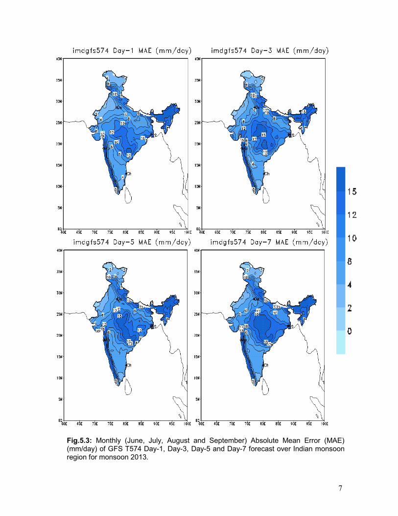
the season. The seasonal Mean Absolute Error (MAE) in mm/day for day-1, day-3 day-5

and day-7 rainfall forecast of GFS T574 over India is shown in Fig.3. The Mean Absolute

Error (MAE) is a scalar measure of forecast accuracy. The MAE is the arithmetic average

of the absolute values of the differences between forecast and observation. Clearly the

MAE is zero if the forecasts are perfect, and increases as discrepancies between the

forecasts and observations become larger. In all days (24 to 168 hr) of forecast, the area

of maximum and minimum MAE is consistent with slight increase in magnitude of MAE

with forecast lead time.

6

Fig.5.2: Monthly (June, July, August and September) Mean Error (mm/day) of GFS T574 Day-1 (top panel), Day-3 (middle pane) and Day-5 (bottom panel) forecast over Indian monsoon region for monsoon 2013.

7

Fig.5.3: Monthly (June, July, August and September) Absolute Mean Error (MAE) (mm/day) of GFS T574 Day-1, Day-3, Day-5 and Day-7 forecast over Indian monsoon region for monsoon 2013.

8

Fig.5.4: Seasonal Root Mean Squared Error (RMSE in mm/day) of GFS T574 Day-1, Day-3, Day-5 and Day-7 Forecast over Indian monsoon region for the period from 1 June 30 September 2013.

9

The spatial distribution of seasonal root mean square error (rmse) rainfall (mm/day)

based on day-1,day-3,day-5 and day-7 forecast of GFS T574 for the period from 1 June

to 30 September 2013 is shown in Fig.5.4. RMSE is a measure of the random component

of the forecast error. The values of rmse are higher over the regions where the daily

rainfall variability is also high. The less rmse over southern peninsular India indicates that

the day to day rainfall variability over this region is also small as compared to other

regions. The rmse of day-1 to day-7 forecasts of the model has a magnitude between 10

and 25 mm, except over the Sub Himalayan West Bengal (SHWB), west coast of India

and central India where the magnitude of rmse exceeds 30 mm. The spatial distribution of

rmse pattern of all day-1 to day-7 forecast is consistent with the area of maximum and

minimum rmse values. The spatial pattern of rmse of the model day-1 to day-5 forecast

shows that the errors are of a more systematic in forecasts lead time.

The Anomaly correlation coefficient (ac) between the observed and the model

forecasts precipitation for day-1 to day-5 of GFS T574 is shown in Fig.5.5. Over most of

the country, the magnitude of day-1 and day-2 anomaly CC lies between 0.3 and 0.5,

while over the monsoon trough regions, the magnitude of anomaly CC exceeds 0.5. A

small area over south west Rajasthan has a magnitude of anomaly CC exceeding 0.6 in

GFS 574 in day-1 to day-3 forecast. The anomaly CC exceeding 0.3 is considered to be

good for precipitation forecast. The spatial distribution of the values of anomaly CC

decreases with longer forecast length. This indicates that the trend in precipitation in the

day-1 to day2 forecasts of the model is in good phase relationship with the observed trend

over a large part of the country. The magnitude of anomaly CC decreases with the

forecast lead time, and by day 5 anomaly CC values over most of India are between 0.1

and 0.2, except in pockets near the east coast and south peninsular India where the

anomaly CC values are below 0.1. The standard WMO method of the verification of

outputs (WMO 1992) is not adequate for precipitation due to its great temporal and spatial

variability. The statistical parameters based on the frequency of occurrences in various

classes are more suitable for determining the skill of a model in predicting precipitation.

10

Fig.5.5: Spatial distribution of anomaly correlation coefficient (ac) between the

observed and the model predicted rainfall for day-1 to day-5 of GFS T574 for the

period from 1 June to 30 September 2013

11

5.1.4.1.3 Rainfall Forecast skill score

The standard WMO method of the verification of outputs (WMO 1992) is not

adequate for precipitation due to its great temporal and spatial variability. The statistical

parameters based on the frequency of occurrences in various classes are more suitable

for determining the skill of a model in predicting precipitation. The aspect of model

behaviour is further explored in Fig.5.6 probability of detection (POD) and Fig.5.7 thread

score (TS) for rainfall threshold of 10 mm/day are presented.

The probability of detection (POD) is equal to the number of hits divided by the total

number of rain observations; thus it gives a simple measure of the proportion of rain

events successfully forecast by the mode. From Fig.5.6, it is seen that the probability of

detection is more than 50% for rainfall threshold value of 10 mm/day for day-1 and day-3

forecast, while it is further below for day-5 and day-7 forecast. It is also seen that skill is a

strong function of forecast lead time (day-1 to day-7) , with the POD decreasing from more

than about 50% in day-1 forecast over most parts of the country to less than 50 % in day-

7 forecast for rain amount of 10 mm/day.

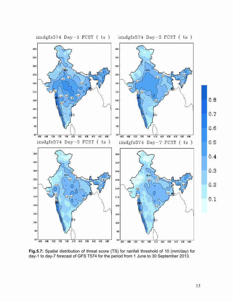
Threat score (TS), also known as the critical success index (CSI, e.g., Schaefer,

1990); or equitable threat score (ETS) which is a modification of the threat score to

account for the correct forecasts due to chance (Gilbert, 1884), is for verification of the

skill in precipitation forecasting. The threat score (TS) is the ratio of the number of correct

model prediction of an event to the number of all such events in both observed and

predicted data. It can be thought of as the accuracy when correct negatives have been

removed from consideration, that is, TS is only concerned with forecasts that count. It

does not distinguish the source of forecast error and just depends on climatological

frequency of events (poorer scores for rarer events) since some hits can occur purely due

to random chance. The higher value of a threat score indicates better prediction, with a

theoretical limit of 1.0 for a perfect model. The threat score (TS) of the model day-1,day-

3,day-5 and day-7 forecasts for monsoon 2013 is shown Fig.5.7. The TS for rainfall

amount of 10 mm/day are more than 0.5 over monsoon trough regions in day-1 forecast.

12

All India : Daily spatial cc : 2012

0

0.2

0.4

0.6

0.8

1 16 31 46 61 76 91 106 121

RA

INF

AL

L in

mm

/day

DAY-1 DAY-2 DAY-3 DAY-4 DAY-5(a)

Fig.5.6: Spatial distribution of POD between the observed and the model predicted rainfall for 10 mm/day, day-1 to day-5 of GFS T574 for the period from 1 June to 30 September 2013.

13

Fig.5.7: Spatial distribution of threat score (TS) for rainfall threshold of 10 (mm/day) for day-1 to day-7 forecast of GFS T574 for the period from 1 June to 30 September 2013.

14

Fig.5.8: Seasonal mean TS and ETS of GFS T574 Day-1 to Day-7 forecast over Indian monsoon region for the period from 1 June 30 September 2013.

The higher value of a threat score indicates better prediction, with a theoretical limit

of 1.0 for a perfect model. The TS and equitable threat score (ETS) of the model day-1 to

day-7 forecasts for monsoon 2013 is shown Fig5.8. The threat score starts close to 0.65

for rainfall threshold of 0.1 mm/day and then decreases to 0.3 near the 10 mm mark.

Interestingly, the day-1 to day-7 threat score follow the same pattern of high score for

rainfall at low threshold and low score for at high rainfall threshold. The TS skill remains

relatively slightly higher in all the threshold ranges. Among the wide variety of

performance measures available for the assessment of skill of deterministic precipitation

forecasts, the equitable threat score (ETS) might well be the one used most frequently.

The ETS is often used in the verification of rainfall in NWP models because its

"equitability" allows scores to be compared more fairly across different regimes.If the ETS

= 1, it indicates that there is no error in the forecasting. ETS = 0 indicates that none of the

grid points are correctly predicted. The ETS skill for the model, day-1 to day-7 forecasts

are ranged between 0.1 to 0.2 for rainfall threshold values of 0.1 to 30 mm/day. GFS has

significant skill for precipitation in lower threshold and it falls off rapidly for larger

precipitation amounts and also for longer lead time.

ETS : MON:2013

0

0.02

0.04

0.06

0.08

0.1

0.12

0.14

0.16

0.18

0.2

0.1 2.5 5 10 15 20 25 30 35 65

mmRainfall threshold in mm

ET

S s

core

DAY-1 DAY-2

DAY-3 DAY-4

DAY-5 DAY-6

DAY-7

Thread Score :MON 2013

0

0.1

0.2

0.3

0.4

0.5

0.6

0.7

0.1 2.5 5 10 15 20 25 30 35 65

mmrainfall threshold in mm

Th

read

Sco

re

Day-1 Day-2

Day-3 Day-4

Day-5 Day-6

Day-7

15

RMSE (mm/day) :Day-1

0

20

40

60

80

1-Ju

n-20

13

6-Ju

n-20

13

11-J

un-2

013

16-J

un-2

013

21-J

un-2

013

26-J

un-2

013

1-Ju

l-201

3

6-Ju

l-201

3

11-J

ul-2

013

16-J

ul-2

013

21-J

ul-2

013

26-J

ul-2

013

31-J

ul-2

013

5-A

ug-2

013

10-A

ug-2

013

15-A

ug-2

013

20-A

ug-2

013

25-A

ug-2

013

30-A

ug-2

013

4-Se

p-20

13

9-Se

p-20

13

14-S

ep-2

013

19-S

ep-2

013

24-S

ep-2

013

29-S

ep-2

013

RM

SE in

mm

/day

.

CI

EI

NE

NW

SP

RMSE (mm/day) :Day-5

0

20

40

60

80

1-Ju

n-20

13

6-Ju

n-20

13

11-J

un-2

013

16-J

un-2

013

21-J

un-2

013

26-J

un-2

013

1-Ju

l-20

13

6-Ju

l-20

13

11-J

ul-2

013

16-J

ul-2

013

21-J

ul-2

013

26-J

ul-2

013

31-J

ul-2

013

5-A

ug-2

013

10-A

ug-2

013

15-A

ug-2

013

20-A

ug-2

013

25-A

ug-2

013

30-A

ug-2

013

4-Se

p-20

13

9-Se

p-20

13

14-S

ep-2

013

19-S

ep-2

013

24-S

ep-2

013

29-S

ep-2

013

RM

SE in

mm

/day

.

CI

EI

NE

NW

SP

RMSE (mm/day) :Day-7

0

20

40

60

80

1-Ju

n-20

13

6-Ju

n-20

13

11-J

un-2

013

16-J

un-2

013

21-J

un-2

013

26-J

un-2

013

1-Ju

l-20

13

6-Ju

l-20

13

11-J

ul-2

013

16-J

ul-2

013

21-J

ul-2

013

26-J

ul-2

013

31-J

ul-2

013

5-A

ug-2

013

10-A

ug-2

013

15-A

ug-2

013

20-A

ug-2

013

25-A

ug-2

013

30-A

ug-2

013

4-Se

p-20

13

9-Se

p-20

13

14-S

ep-2

013

19-S

ep-2

013

24-S

ep-2

013

29-S

ep-2

013

RM

SE in

mm

/day

.

CI

EI

NE

NW

SP

RMSE (mm/day) :Day-3

0

20

40

60

80

1-Ju

n-20

13

6-Ju

n-20

13

11-J

un-2

013

16-J

un-2

013

21-J

un-2

013

26-J

un-2

013

1-Ju

l-20

13

6-Ju

l-20

13

11-J

ul-2

013

16-J

ul-2

013

21-J

ul-2

013

26-J

ul-2

013

31-J

ul-2

013

5-A

ug-2

013

10-A

ug-2

013

15-A

ug-2

013

20-A

ug-2

013

25-A

ug-2

013

30-A

ug-2

013

4-Se

p-20

13

9-Se

p-20

13

14-S

ep-2

013

19-S

ep-2

013

24-S

ep-2

013

29-S

ep-2

013

RM

SE in

mm

/day

.

CI

EI

NE

NW

SP

Fig.5.9: Time series of daily all India domain mean RMSE (mm/day) of day-1, day-3,

day-5 and day-7 forecast during monsoon 2013.

16

The daily time series of all India domain mean RMSE (mm/day) of day-1, day-3,

day-5 and day-7 forecast over Indian monsoon region for the period from 1 June 30

September 2013 is shown in Fig.5.9. GFS T574 shows the daily mean RMSE in the

range of 15 -20 mm/day for all India, while it is varying from 25 -30 mm/day for central

India in day-1 to day-7 forecast. For the north-east and west coast of India, the RMSE is in

the range of 15-20 mm/day. The magnitude of RMSE over southern peninsular India is

small in all day-1 to day-7 during monsoon 2013.The seasonal mean daily rainfall over

NE, WC and central India regions are high as compared to other regions of India. Hence,

the higher rainfall over these regions leads to higher values of RMSE during monsoon

season. In general, the daily RMSE is relatively high in all the regions and in all day-1 to

day-7 forecast during July and August as compared June and September months. The

seasonal mean RMSE of GFS T574 Day-1 to Day-7 forecast over Indian monsoon region

for the period from 1 June 30 September 2013 is shown in Fig.5.10. The daily domain

average RMSE is high for central, west coast of India and NE India regions and relatively

small for the southern peninsular India region in all day-1 to day-7 forecasts during the

monsoon periods 1 June - 30 September 2013.

RMSE

0

5

10

15

20

25

30

35

A-India CE EI NE NW SP WC

RM

SE

in

mm

/da

y

DAY-1

DAY-2

DAY-3

DAY-4

DAY-5

DAY-6

DAY-7

Fig.5.10: seasonal mean RMSE of GFS T574 Day-1 to Day-7 forecast over Indian monsoon region for the period from 1 June 30 September 2013.

17

SPATIAL CC :MONSOON 2013

00.2

0.4

0.6

0.8

1-J

un

-20

13

8-J

un

-20

13

15

-Ju

n-2

013

22

-Ju

n-2

013

29

-Ju

n-2

013

6-J

ul-

201

3

13

-Ju

l-2

01

3

20

-Ju

l-2

01

3

27

-Ju

l-2

01

3

3-A

ug

-20

13

10

-Au

g-2

013

17

-Au

g-2

013

24

-Au

g-2

013

31

-Au

g-2

013

7-S

ep-2

01

3

14

-Sep

-20

13

21

-Sep

-20

13

28

-Sep

-20

13

Sp

atia

l C

C

Day-1 (0.124)

Day-3 (0.126)

Day-5 (0.110)

Day-7 (0.106)

Spatial CC :ALL INDIA

0

0.05

0.1

0.15

0.2

0.25

0.3

0.35

Day-1 Day-2 Day-3 Day-4 Day-5 Day-6 Day-7

CC

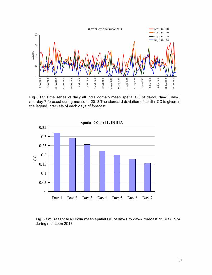
Fig.5.11: Time series of daily all India domain mean spatial CC of day-1, day-3, day-5 and day-7 forecast during monsoon 2013.The standard deviation of spatial CC is given in the legend brackets of each days of forecast.

Fig.5.12: seasonal all India mean spatial CC of day-1 to day-7 forecast of GFS T574 during monsoon 2013.

18

The time series of daily all India domain mean spatial CC of GFS T574 day-

1, day-3, day-5 and day-7 forecast and its standard deviation of spatial CC during

monsoon 2013 is given in Fig.11. The standard deviation is given in the legend

brackets of each days of forecast. The daily time series of spatial correlation

coefficient (CC) shows that the spatial CC is high in day-1 and decreases with

forecast lead time. The daily spatial CC for day-1 forecast is varying from 0.3 to

0.6 and its mean value is around 0.35. For day-5 forecast, the CC is oscillating

between 0.2 to 0.4 and mean is around 0.20 and standard deviation is 0.110 .The

daily mean spatial CC is falling from 0.35 in day-1 to 0.15 in day-7 forecasts over

Indian monsoon regions. The day-1 and day-3 spatial CCs are higher and is in the

acceptable significant level. The seasonal mean all India mean spatial CC of day-1

to day-7 forecast of GFS T574 during monsoon 2013 is shown in Fig.5.12. The

domain average spatial CC is 0.35 for day-1 and became 0.15 in day-7 forecast.

The value of spatial CC decreases with forecast lead time.

5.1.4.2 Monsoon Circulation Features

5.1.4.2.1 Seasonal Mean wind pattern

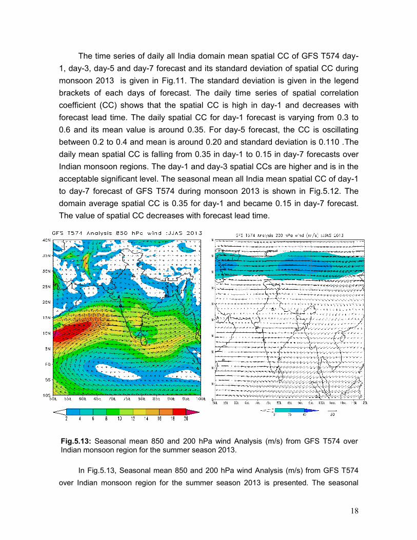
In Fig.5.13, Seasonal mean 850 and 200 hPa wind Analysis (m/s) from GFS T574

over Indian monsoon region for the summer season 2013 is presented. The seasonal

Fig.5.13: Seasonal mean 850 and 200 hPa wind Analysis (m/s) from GFS T574 over Indian monsoon region for the summer season 2013.

19

(JJAS) mean wind analysis could capture low level westerly jet with a peak strength over

the south west Arabian sea and the monsoon trough extending from northwest Bay of

Bengal to northwest wards across the country. During the early summer months,

increased solar heating begins to heat the Indian subcontinent, which would tend to set up

a monsoon circulation cell between southern Asia and the Indian Ocean. However, the

subtropical jet stream occupies its winter position at about 30° N latitude, south of the

Himalayan Mountains (Fig.5.13). As summer progresses, the subtropical jet slides

northward. The extremely high Himalayas present an obstacle for the jet; it must "jump

over" the mountains and reform over central Asia. When it finally does so, a summer

monsoon cell develops, supported by the tropical jet stream overhead.

In Fig.5.14, Seasonal mean wind (at 850 hPa) Error (m/s) of GFS T574 day-1, day-

3, day-5 and day-7 forecast over India during monsoon 2013 is presented. GFS T574

forecast shows bias of westerly wind over most parts of the parts of country extending up

to the foot hills (indicating weak monsoon trough) south-westerly bias over the north west

India and northeast Arabian sea, and northerly bias over east coast of India and adjuring

Bay of Bengal extending southwards up to 15o N in July and August month. Over the

Myanmar it has been westerly bias. The magnitude of bias is found to grow with the

forecast lead time. The westerly bias over NE Arabian Sea and adjoining Gujarat coast is

found to be slightly stronger in the day3 and day-5 forecast during July and August. The

monthly mean 200 hPa wind Analysis and Error (m/s) (200 hPa) from GFS T574 over

Indian monsoon region for the month of June, July and August 2013 depicted in Fig.5.15.

The subtropical jet stream occupies its position over India during June is around 35° N

latitude, north of the Himalayan Mountains. As summer progresses, the subtropical jet

slides northward and located around 40° N in July and 45° N in August 2013. The day-3

and day-5 forecast during July and August have easterly bias north of 20° N over India

and southwesterly bias over SW Arabian Sea during July and August month.

20

Fig.5.14: Seasonal 850 hPa wind Error (m/s) from GFS T574 day-1, day-3, day-5 and day-7 forecast over India during monsoon 2013.

21

Fig.5.15: Seasonal 200 hPa wind Error (m/s) from GFS T574 day-1, day-3, day-5 and day-7 forecast over India during monsoon 2013.

22

5.1.4.2.2 Forecast Error in Specific humidity

Fig.5.16: Vertical cross-section of Long (68 -98 E) averaged GFS T574 specific humidity Error (g/kg) over Indian monsoon region for the period from 1 June 30 September 2013.

23

In Fig.5.16, zonally averaged (long 60o E to 100o E) vertical cross-section specific

humidity (g /kg) of day-1, day-3, day-5 and day-7 forecast errors from GFS T574 for

monsoon 2013 is presented. In order to understand the characteristic features of

monsoon captured by the model, the model performance is examined in terms of vertical

structure of zonally averaged (long 60o E to 100o E) specific humidity error (bias) at 77o E

during 1 June to 30 September 2013. The specific humidity error analysis shows similar

pattern with under estimation of specific humidity below 600 hPa. GFS T574 forecast

errors shows negative bias between 850 hPa and 600 hPa, extending northward up to

30o N with two minima, one at the equator and another between 15 o N - 20 o N around

800 hPa. In the lower levels from surface between lat 10o N and 15o N, there is a

negative bias of specific humidity. Above 550 hPa, the error is positive with a maximum

value between 600 hPa and 500 hPa and Lat 10o N -15 o N. The magnitude of bias

increases with the forecast lead time

5.2 Performance of Operational WRF Model during Southwest Monsoon 2013

This section of the report discusses about the performance of Weather Research

and Forecast (WRF) model operational at India Meteorological Department, New Delhi

during monsoon 2013. The verification of the forecasts has been conducted as per the

availability of verification analyses which are the rainfall analysis (0.5oX0.5o) of IMD and

mesoscale analyses generated through WRFDA assimilation system. The study covered

continuous scores and a few categorical scores for rainfall forecast over whole India and

over seven selected zones. The standard spatial error maps for a few meteorological

variables have been produced relevant to performance verification.

Along with its assimilation component WRF Data Assimilation (WRFDA), the

mesoscale modeling system is in operation in IMD for short-range forecasting of weather

events up to three days. The performance verification of the WRF forecasts has been

carried out in the annual reports of monsoon published in IMD from the year 2010 to 2013

(Das, et al., 2011). The standard well known scores have usually been computed

especially for quantitative precipitation forecast (QPF). Other parameters have also been

evaluated through diagnostic methods for better understanding of the errors. The

verification practice in IMD using continuous and categorical scores within a framework of

neighborhood technique has limitation in evaluating model performance at higher

resolution (Hogan et al., 2010). But, the use of advanced diagnostic methods of

verification is restricted due to the unavailability of reference data set (observations or

verification analyses) with a reasonable resolution (temporal and spatial) to match the

24

resolution of model forecasts. The NWP division in IMD, New Delhi every year carries out

standard verification exercises for different model forecasts (generated or utilized) during

southwest monsoon season. This present report only focuses on evaluation of real-time

forecasts of WRF model during southwest monsoon 2013.

During southwest monsoon season 2013, the WRF model (ARW) with its double

nested configuration has been operational to deliver three days forecasts twice daily at 00

UTC and 12 UTC. The data assimilation component, WRF Data Assimilation (WRFDA)

takes global GFS analysis and all other quality controlled observations as its input and

generates mesoscale analysis. The analyses with modified boundary condition (available

from GFS) are then provided to WRF model for operational forecasting. The model

domains (mother - 27 km and a nested domain - 9 km) covered the area of responsibility

for Regional Specialized Meteorological Center (RSMC), New Delhi and Indian region

respectively. The observational data from GTS and other sources after decoding and

quality control has been preprocessed to create PREPBUFR files (in NCEP-BUFR format)

which is used as an input to WRFDA system. Observations are accumulated within ±3

hour time-window from a specific hour to generate corresponding PREPBUFR file. In the

assimilation system, all conventional observations over a domain (20o S to 45o N; 40o E to

115o E) have been ingested to create improved mesoscale analysis.

WRF model is a non-hydrostatic high-resolution mesoscale model. The model has

been configured with full physics for during day to day operational run. The summary of

the model configuration used for operational purpose in IMD is given in table 1. The detail

description can be found out in the relevant model documentation (WRF, 2011)

maintained by National Center for Atmospheric Research (NCAR), USA.

The post-processing programs WPP (WRF Post Processor) and NCL (NCAR

Command Language) package have been utilized for the processing of model forecasts

so that it can utilized by the MET (Model Evaluation Tools). WPP program converted WRF

forecasts to grib2 format and NCL prepared “netcdf” files for observed and forecast

rainfall.

The performance evaluation has been carried out with verification analyses

available during the period. Rainfall analyses (Mitra et al., 2009) were available at 0.5o

resolution at National Data Center, IMD Pune. A sub-domain over Indian region (specified

by latitude range 6.5o N to 38.5o N and longitude range 66.5o E to 100.5o E) has been

considered for concrete verification over the region. The accumulation period of the

rainfall forecast has been matched with the verification analysis which is from 03 UTC of a

25

day to 03 UTC of next day. The scope of verification of WRF-ARW model has been

restricted only to mother

The categorical verification scores along with standard continuous scores for rainfall

have been computed to evaluate model performance. The different rainfall categories are

defined on the basis of the classification used in India Meteorological Department

(described in table 3). In this study, last two categories above heavy rain class are not

considered for the verification purpose. In this document, categorical skill scores, Critical

Success Index (CSI or threat score), BIAS score (FBIAS) and Gilbert Skill Score (GSS or

equitable threat score) have been computed over seven specified zones and over India as

a whole. The standard scores e.g. mean error (ME) and root mean square error (RMSE)

have also been calculated for verification. The locations and extents of seven selected

zones are shown in figure 17 and their description has been given in table-5.2.

The relevant description on the spatial error patterns for mean sea level pressure,

and wind at 850 and 200 hPa has been added along with rainfall forecast verification. The

error in model forecast averaged over a month has been analyzed to bring out

inadequacies of the model to portray monsoon circulation in a realistic manner. Spatial

distribution of mean error and RMSE only for middle monsoon months July and August

have been described. The elaboration for very much relevant parameters e.g.

temperature, relative humidity and geopotential height have been skipped to shorten the

length of the report. Many figures in results and discussion section have been dropped

due to obvious supposition projected from the existing figures.

5.2.1 Results and Discussion

The discussion of the report is collectively partitioned in three parts described below.

Although, three partitions are separated by notion for better readability but time to time the

obvious linkages are put forth within the write up of each portion.

a) Verification of rainfall

(i) The evaluation of daily rainfall forecasts series averaged over country as a whole

during southwest monsoon season 2012 against observation and climate normal.

(ii) Continuous scores and categorical skill scores for different rainfall threshold are

calculated over India and over other seven specified zones.

b) Verification of wind components and mean sea level pressure (MSLP), relative

humidity, temperature and geopotential height at 500 hPa.

26

Verification of Rainfall

(i) Times series of daily rainfall has been derived for observation and WRF forecasts

for three days. The average over Indian domain mentioned in earlier section has been

done to calculate the daily rain rate over the country as a whole. The figure 18,

representing daily time series of all India rainfall rates. Vertical bars in green gives

observed rainfall time series along with daily normal value plotted in red curve. Other lines

of the figure shows the daily rainfall rates in day 1, day 2 and day 3 forecasts which are

plotted along with observed and normal values. It was evident that the forecast series

could not capture reasonably the lull periods of the season in which observed rainfall was

below normal. The active i.e. the peaks in the observed field has never been missed in the

model forecasts. The day 1 forecast has larger tendencies to overestimate all India rainfall

merely throughout the season compared to other forecast hours. Model produced daily

rainfall rate gradually decreases along with forecast hours. The days with peaks rain

spells are fairly detected but sharp drops for certain days have been missed out by the

model.

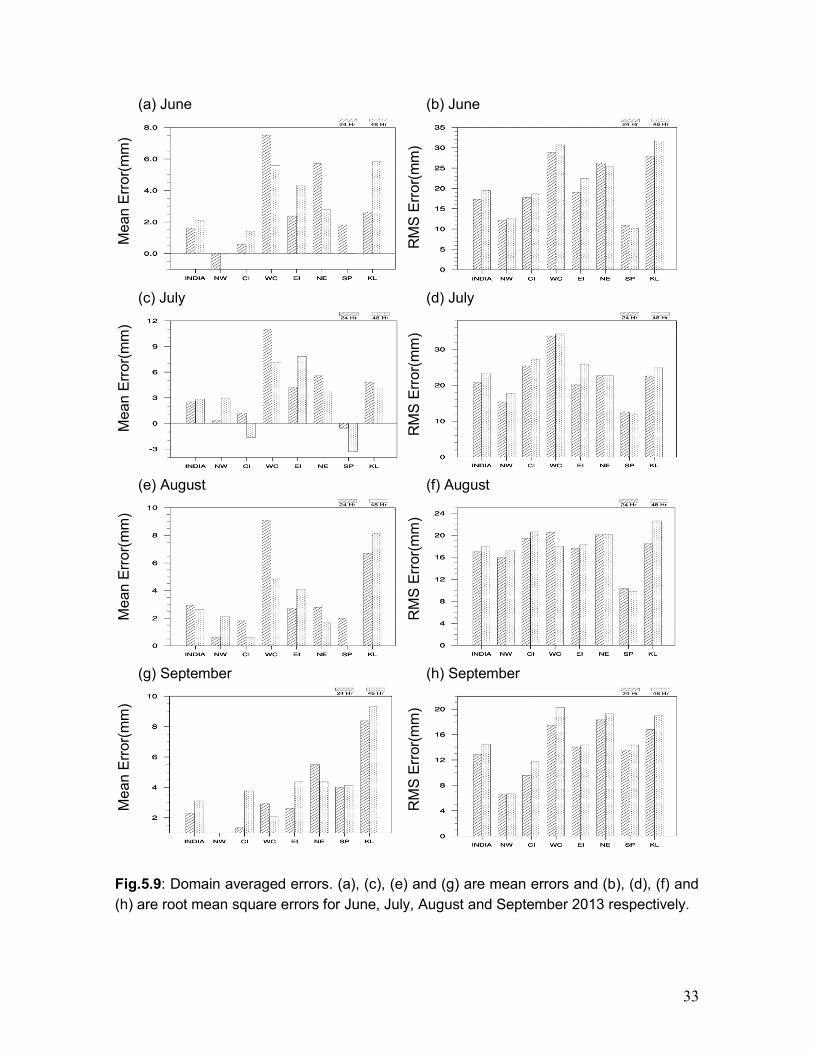
(ii) Fig.19a and Fig.19.b give concise representation of errors over seven different

zones and India for June. Mean error tells that the overestimation is prevalent over the

regions with higher rainfall e.g. over KRL, WC and NE India. RMSE values are also higher

for the zones with higher rainfall as ME contribute hugely in that and it reduces in the later

months of the monsoon season. Only NW zone is showing underestimation as the rainfall

during June over the region has been contributed hugely by pre-monsoon

thundershowers. Figure 19c and d have summarized the fact for July in terms of ME and

RMSE. ME shows the overestimation all over India in day 1 forecast. The tendency of

positive bias for the higher rainfall belts persists as it has been seen in June. The mean

errors have low values over CI and SP zone. The lower values of RMSE over SP but

higher over CI indicates that the forecasts are consistent over southern peninsula and

randomness prevails over central India. Overall decrease in errors can be seen in August

and September. In September, as the rainfall amount reduces over India due to

withdrawal of monsoon, the errors decrease except comparatively large overestimation

over Kerala. The error values over central zones suggests that the rainfall belt generated

due to migrating low pressure systems have been forecasted well by the model in day 1

forecast although the localized areas of highest rain might not been forecasted accurately

as the categorical skill scores deteriorated in categories for higher rain (Fig.5.20). The

continuous scores for whole India gives an impression that the model prediction has a

tendency of overestimation. But, while the categorical skill have been considered for

27

different rain threshold and averaged over grid points in the region, the model

performance for higher rain categories have been found to contradict the general notion.

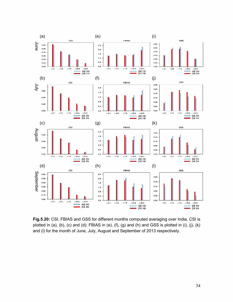
The Fig.5.20 shows the CSI, FBIAS and GSS for four monsoon months considering

five rain categories. Left panels in the figure show the CSI values for all categories and

only two forecast hours (day 1 and 2) have been considered for discussion. CSI score in

every month depict that the forecast quality deteriorates with increasing rain threshold. On

the basis of CSI, it may also be inferred that the model forecasted poorly for the starting

month of June compared to other months as the month has lower number rainy days over

the grid points throughout the region. But, FBIAS and GSS shows the forecasts for June

have comparable accuracy along with other months. Two most rainy months July and

August resemble similar kind of model performance. CSI score for the month of

September show moderate decline in model performance. The better score for lower rain

threshold may be biased with correct “no rain” forecasts. In this regard, GSS score

signifies the real worthiness of forecasts in medium rain categories as the taller bars can

be found for those categories. FBIAS values for every category is more than 1.0 and

higher values for higher rain categories. This illustrates overestimation tendency of the

model for any rain amount. The lower values of GSS in the categories with lower rain

values implicate that the forecasts of rainy days over several grid points are found to be

correct by chance. But, the heavy rainfall points have been either missed or misplaced in

the model forecasts. GSS score reflects no marked month to month variation in model

efficiency. In every skill scores, day 1 and 2 produced comparable performances but up to

medium rainfall categories day 2 forecast found to be marginally better than day 1. As CSI

values drop below 0.3 and GSS below 0.1 after rather heavy rainfall category, the model

forecast cannot be considered reliable. But, the high resolution forecasts have a practical

tendency to generate localized spatial distribution of heavy rainfall. The comparison of the

said forecast (even after up scaling) with low resolution reference (observation) analyses

has an evident drawback of smoothing. On the other hand, grid-point by grid-point

verification method suffers with double penalty with a displaced zone of rainfall occurred in

the forecast compared with observation analysis. Spatial variations of skill have been

examined thereafter to assess the strength and weakness over any certain area. Figure

21 gives skill scores for two different rain categories above 7.5 mm and 35.5 mm

averaged over whole India and over seven specific zones as well. The scores over

individual zones show variation and deteriorate with an increase in rain amount. The

model shows consistent degradation of forecast accuracy for a few zones for all rainfall

28

categories e.g. SP, EI, and NE zones. Whereas, the established forecast accuracy has

been maintained over west coast and Kerala.

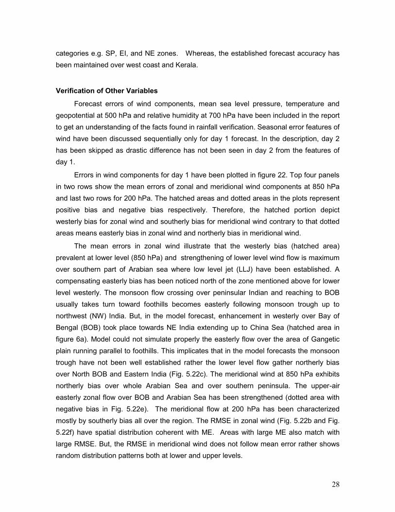
Verification of Other Variables

Forecast errors of wind components, mean sea level pressure, temperature and

geopotential at 500 hPa and relative humidity at 700 hPa have been included in the report

to get an understanding of the facts found in rainfall verification. Seasonal error features of

wind have been discussed sequentially only for day 1 forecast. In the description, day 2

has been skipped as drastic difference has not been seen in day 2 from the features of

day 1.

Errors in wind components for day 1 have been plotted in figure 22. Top four panels

in two rows show the mean errors of zonal and meridional wind components at 850 hPa

and last two rows for 200 hPa. The hatched areas and dotted areas in the plots represent

positive bias and negative bias respectively. Therefore, the hatched portion depict

westerly bias for zonal wind and southerly bias for meridional wind contrary to that dotted

areas means easterly bias in zonal wind and northerly bias in meridional wind.

The mean errors in zonal wind illustrate that the westerly bias (hatched area)

prevalent at lower level (850 hPa) and strengthening of lower level wind flow is maximum

over southern part of Arabian sea where low level jet (LLJ) have been established. A

compensating easterly bias has been noticed north of the zone mentioned above for lower

level westerly. The monsoon flow crossing over peninsular Indian and reaching to BOB

usually takes turn toward foothills becomes easterly following monsoon trough up to

northwest (NW) India. But, in the model forecast, enhancement in westerly over Bay of

Bengal (BOB) took place towards NE India extending up to China Sea (hatched area in

figure 6a). Model could not simulate properly the easterly flow over the area of Gangetic

plain running parallel to foothills. This implicates that in the model forecasts the monsoon

trough have not been well established rather the lower level flow gather northerly bias

over North BOB and Eastern India (Fig. 5.22c). The meridional wind at 850 hPa exhibits

northerly bias over whole Arabian Sea and over southern peninsula. The upper-air

easterly zonal flow over BOB and Arabian Sea has been strengthened (dotted area with

negative bias in Fig. 5.22e). The meridional flow at 200 hPa has been characterized

mostly by southerly bias all over the region. The RMSE in zonal wind (Fig. 5.22b and Fig.

5.22f) have spatial distribution coherent with ME. Areas with large ME also match with

large RMSE. But, the RMSE in meridional wind does not follow mean error rather shows

random distribution patterns both at lower and upper levels.

29

Fig.5.23 is attributed to error features of MSLP and relative humidity at 700 hPa.

The top two panels shows ME of MSLP and RH for day 1 averaged over whole season.

The pressure depression bias is widespread over whole monsoon region which intensifies

towards northern latitudes which increases in day 2. The bias did not show uniform nature

but with comparative lower values over central India and Sri Lanka. In turn a comparative

high formation is noticed in mean error over CI. This probably nudges the rainfall pattern

towards overestimation. Although, monsoon flow along with pressure depression bias in

MSLP stimulate strong monsoon but the negative bias in relative humidity at 700 hPa

shows that the model has a dry bias in lower tropospheric levels. On contrary, the

moistening bias over Somali jet region over Arabian Sea suggests the model has to be

tuned for proper distribution of moisture in lower levels.

Seasonal mean errors for temperature and geopotential at mid-tropospheric level

(500 hPa) have been plotted in Fig. 5.24. Whole monsoon area at 500 hPa is

characterized by warm bias in the model forecast which remains nearly unchanged from

day 1 to day 2. Cooling bias takes place over Tibetan high, Arab and south-east Asia. The

warming a bias produced in model forecast has a nominal value ~ 0.4o C but

comparatively cooling is mild with a value ~ 0.2o C. Geopotential has a –ve bias consistent

with warm bias (Fig. 23b and d) over the region. Higher values of mean error over central

India suggests the model cause zone of high GPH at the vicinity of low (over central and

peninsular India) generally caused due to monsoon lows. The outward height gradient

from central India decreases from day 1 to day 2 forecast (Fig. 23b and d). Location low

GPH established due to migrated monsoon lows has not been properly demonstrated in

model forecasts.

5.6 Summary and Concluding remarks

This report assesses the performance of GFS T574 over Indian region in spatial and

temporal scale during summer monsoon season of 2013. The verification of rainfall is

done in the spatial scale of 50 km, in a spatial scale and also country as a whole in terms

of skill scores, such as mean error, root mean square error, correlation efficient, time

series and categorical statistics such as, POD, TS and ETS. The study demonstrates that

the performance of GFS T574 in predicting rainfall varies with geographical location and

synoptic regime. Magnitude of RMSE is found to be slightly higher for GFS T574,

indicating higher variability in the performance of the model. Validation results show that

the T574 forecasts, in general, is skillful over the regions of climatologically heavy rainfall

domains. Performance of the model is also examined in terms of tropospheric wind

circulation and vertical cross section of specific humidity bias to understand the monsoon

30

rainfall features captured by the model. The skill of wind forecast of the model during

monsoon season is also examined. From the result presented above, the following

Conclusions may be drawn. The observed variability of daily mean precipitation over India

is reproduced remarkably well by the day-1 to day-7 forecasts of GFS T574. It also have

reasonably good capability to capture large scale rainfall features of summer monsoon,

such as heavy rainfall belt along the west coast, over the domain of monsoon trough and

along the foot hills of the Himalayas. In general, GFS T574 showed considerable skill in

predicting the daily rainfall over India during monsoon periods.

In general, the performance verification of WRF model shows that the model has a

consistent tendency of over prediction in rainfall. The positive bias in the rainfall

distribution shows systematic nature for each specific zone in every months of monsoon.

Therefore, bias correction is a viable option to improve forecast quality. The shift due to

irregular movement of low pressure systems from Bay of Bengal towards land has been

depicted to be a consistent limitation of the model forecasts. The wind biases found in the

forecasts indicated the fact the evolution of large scale monsoon systems within monsoon

environment have also not been captured well by the model. The dynamics of the WRF

model may be improved for better prediction of weather systems in terms of monsoon

lows.

Table-5.1 WRF model configuration summary.

Characteristic feature Selected configuration

Double nested domains

Horizontal resolution

27 Km outer domain and 9 km inner domain

Horizontal grid Arakawa C grid (staggered)

Vertical coordinate Terrain following 38 σ levels (staggered)

Time integration Third order Runge-Kutta Scheme

Cloud Microphysics WRF single moment 5-class cloud microphysics

Cumulus convection Grell 3 dimensional ensemble cumulus physics scheme

Planetary boundary layer Mellor-Yamada-Janjic planetary boundary layer scheme

Short-wave radiation

Long-wave radiation

Goddard short-wave radiations physics

Radiation Rapid radiative transfer model (RRTM) long-wave

Land-surface model Eta and Noah Land Surface Model for surface physics

31

Table-5.2 Seven geographical regions considered for rainfall verification

Zone

Name

Geographical Region

of India

Abbreviated

name

Zone 1 Kerala KRL

Zone 2 West Coast WC

Zone 3 Southern Peninsula SP

Zone 4 Central India CTR or CI

Zone 5 East India EI

Zone 6 North-East India NE

Zone 7 North-West India NW

Table-5.3 Classification of Rainfall based on intensity

Descriptive Term Rainfall amount in mm

No Rain 0.0

Very light Rain 0.1- 2.4

Light Rain 2.5 – 7.5

Moderate Rain 7.6 – 35.5

Rather Heavy 35.6 – 64.4

Heavy Rain 64.5 – 124.4

Very Heavy Rain 124.5 – 244.4

Extremely Heavy Rain ≥ 244.5

Exceptionally Heavy

Rain

When the observation is near about the highest recorded

rainfall at or near the station for the month or season.

However, this term will be used only when the actual

rainfall exceeds 120 mm.

32

Fig.5.17: Locations of seven geographical regions for rainfall verification along with GPCC

climate normal rainfall in mm/day.

Fig.5.18: All India daily rainfall time series during southwest monsoon season 2013.

33

(a) June (b) June

M

ean E

rro

r(m

m)

RM

S E

rro

r(m

m)

(c) July (d) July

M

ean E

rro

r(m

m)

RM

S E

rro

r(m

m)

(e) August (f) August

M

ean E

rro

r(m

m)

R

MS

Err

or(

mm

)

(g) September (h) September

M

ean E

rro

r(m

m)

R

MS

Err

or(

mm

)

Fig.5.9: Domain averaged errors. (a), (c), (e) and (g) are mean errors and (b), (d), (f) and

(h) are root mean square errors for June, July, August and September 2013 respectively.

34

(a) (e) (i)

Ju

ne

(b) (f) (j)

Ju

ly

(c) (g) (k)

Au

gu

st

(d) (h) (l)

Se

pte

mb

er

Fig.5.20: CSI, FBIAS and GSS for different months computed averaging over India. CSI is

plotted in (a), (b), (c) and (d); FBIAS in (e), (f), (g) and (h) and GSS is plotted in (i), (j), (k)

and (l) for the month of June, July, August and September of 2013 respectively.

35

(a) (d)

(b) (e)

(c) (f)

Fig.5.21: Mean values of CSI, FBIAS and GSS during whole monsoon season 2013

which are computed averaging over all India and other seven selected zones. (a) CSI, (b)

BIAS and (c) GSS for rainfall category greater than 7.5 mm; (d), (e) and (f) represent the

same for the category > 35.6 mm.

36

(a) ME of U at 850 hPa (b) RMSE of U at 850 hPa

(c) ME of V at 850 hPa (d) RMSE of V at 850 hPa

(e) ME of U at 200 hPa (f) RMSE of U at 200 hPa

(g) ME of V at 200 hPa (h) RMSE of V at 200 hPa

37

Fig.5.22: Day 1 forecast errors in wind components (a), (b) and (c), (d) at 850 hPa; (e), (f)

and (g), (h) at 200 hPa for u wind and v wind respectively.

(a) Day 1 ME in MSLP (hPa) (b) Day 1 ME in RH (%)

(c) Day 2 ME in MSLP (hPa) (d) Day 2 ME in RH (%)

Fig.5.23: Spatial distribution of seasonal mean errors in MSLP and relative humidity at

700 hPa. (a) And (b) for day 1 and (c) and (d) for day 2 respectively.

(a) Day 1 ME of T (o C) at 500 hPa (b) Day 1 ME of GPH at 500 hPa

38

(c) Day 2 ME of T (o C) at 500 hPa (d) Day 2 ME of GPH at 500 hPa

Fig.5.24: Spatial distribution of seasonal mean errors in temperature and geopotential

height at 500 hPa. (a) And (b) for day 1 and (c) and (d) for day 2 respectively.

References

Das A K, M Rathee, M Bhowmick, H Fatima, 2011 : WRFDA and WRF-ARW

Modelling system at IMD –HQ. Annual NWP performance report 2010. IMD Met.

Monograph No. NWP/Annual Report/01/2011

Durai V.R. and Roy Bhowmik, S.K., 2013, Prediction of Indian summer monsoon in

short to medium range time scale with high resolution global forecast system (GFS) T574 and T382, Climate Dynamics 2013, online DOI No. 10.1007/s00382-013-1895-5

Durai V R , Roy Bhowmik S K and Mukhopadhaya B., 2010a “Performance

Evaluation of precipitation prediction skill of NCEP Global Forecasting System (GFS) over Indian region during Summer Monsoon 2008” Mausam 2010, 61(2), 139-154

Durai V R, Roy Bhowmik S K and Mukhopadhaya B., 2010b “Evaluation of Indian summer monsoon rainfall features using TRMM and KALPANA-1 satellite derived precipitation and rain gauge observation” Mausam 2010, 61(3), 317-336

Hogan R J, Christopher A T F, I T Jolliffe, D B Stephenson, 2010: Equitability

revisited: Why the „equitable threat score‟ is not equitable. Wea Forecasting, 25, 710-726

39

Kalnay, M. Kanamitsu, and W.E. Baker, 1990: Global numerical weather prediction at the National Meteorological Center. Bull. Amer. Meteor. Soc., 71, 1410-1428.

Kanamitsu, M., 1989: Description of the NMC global data assimilation and forecast system. Weather and Forecasting, 4, 335-342.

Kanamitsu, M., J.C. Alpert, K.A. Campana, P.M. Caplan, D.G. Deaven, M. Iredell, B. Katz, H.-L. Pan, J. Sela, and G.H. White, 1991: Recent changes implemented into the global forecast system at NMC. Weather and Forecasting, 6, 425-435.

MET version 3.0 comprehensive user documentation. (2011) January,

Developmental Testbed Center, Boulder, USA, (Available online at

http://www.dtcenter.org/met/users/docs/users_guide/MET_Users_Guide_v3.0.2.pdf

Mitra A K, A K Bohra, M N Rajeevan and T N Krishnamurti, 2009: Daily Indian

precipitation analysis formed from a merge of rain-gauge data with the TRMM TMPA

satellite-derived rainfall estimates. J Met Soc Japan, 87A, 265-279

Roy Bhowmik ,S.K., V.R. Durai, Ananda K Das and B. Mukhopadhaya, Performance of IMD Multi-model Ensemble based District Level Forecast System during Summer Monsoon 2008, Met Mon No. synoptic meteorology 8/2009, 43 pp, India Meteorological Department.

WRF ARW Version 3 Modeling System User‟s Guide. (2011) April, Mesoscale &

Microscale Meteorology Division, National Center for Atmospheric Research, USA,

Available online at http://www.mmm.ucar.edu/wrf/users/docs/arw_v3.pdf