Copyright © 2006, 2009 by Andrei Hagiu

Working papers are in draft form. This working paper is distributed for purposes of comment and discussion only. It may not be reproduced without permission of the copyright holder. Copies of working papers are available from the author.

Monopolistic Competition Between Differentiated Products With Demand For More Than One Variety Andrei Hagiu

Working Paper

09-095

Monopolistic Competition Between Differentiated Products

With Demand For More Than One Variety

Andrei Hagiu∗

July 15 2006

Abstract

We analyze the existence of pure strategy symmetric price equilibria in a gener-

alized version of Salop (1979)’s circular model of competition between differentiated

products - namely, we allow consumers to purchase more than one brand. When con-

sumers purchase all varieties from which they derive non-negative net utility, there is no

competition, so that each firm behaves like an unconstrained monopolist. When each

consumers is interested in purchasing an exogenously given number (n) of varieties, we

show that there is no pure strategy symmetric price equilibrium in general (for n > 2

with linear transportation costs). In turn, if the limitation on the number of varieties

consumers purchase comes from a budget constraint then we obtain a multiplicity of

symmetric price equilibria, which can be indexed by the number of varieties consumers

purchase in equilibrium.

Keywords: Monopolistic competition, Product Variety.

JEL Classifications: L1, L2, L8

∗Harvard Business School, ahagiu@hbs.edu

1. Introduction

We are interested in developing a theoretical framework for studying price competition

between multiple firms, with the following characteristics: (i) firms offer differentiated

products; (ii) consumers have unitary demand for any given product, i.e. every consumer

will buy either 0 or 1 units of any brand; (iii) consumer preferences are heterogeneous and

"localized" in the sense that they differ in the identity of their ideal brand and each con-

sumer values brands less the further they are in preference space from his ideal brand; (iv)

each consumer is potentially interested in buying more than one product. Two examples

of markets which fit the description outlined by the four points above are software applica-

tions and videogames. There are thousands of software applications as well as games, and

different users are interested in different applications/games. A given software or game

user’s tastes may overlap with another’s, yet they may have nothing in common with a

third’s. Thus, although there is a sense in which competition is localized (any given firm

competes only with firms, whose brands are similar to its own), it is not clear how the fact

that consumers are generally interested in purchasing multiple products affects the type of

competition waged among firms.

We are motivated by the observation that the two main standard models of monopo-

listic competition do not seem to be well-suited for illustrating this type of competition.

Indeed, the spatial framework proposed by Salop (1979) treats competition as a localized

phenomenon and satisfies conditions (i) through (iii) above, but not (iv): each consumer

is interested in purchasing a single brand. In turn, the representative consumer framework

of Spence (1976) and Dixit and Stiglitz (1977) satisfies (iv) (consumers purchase positive

quantities of all brands), but not (i), (ii) and (iii) (all products are interchangeable for all

consumers). Subsequent papers have generalized each of these models and derived more

2

solid foundations for their basic assumptions (Sattinger (1984), Perloff and Salop (1985)).

There have also been some theoretical attempts to reconcile the two frameworks, the most

significant of which is Deneckere and Rotschild (1992). However, none of them has specifi-

cally studied price competition in a setting combining the consumer heterogeneity, localized

competition and unitary demand per brand features of spatial models with the preference

for diversity (demand for multiple products) property of the symmetric aggregate demand

formulation.

The framework we propose combines features from both strands of the literature in

the following way. We take Salop’s circle representation of consumer preferences and firms’

locations as the starting point for our model and make the important modifying assumption

that each consumer is interested in purchasing several brands, rather than just one.

Therefore all the action in our model depends on what we assume it is that determines

how many varieties are purchased. We investigate three possibilities. The first variant

of our model postulates that each consumer purchases all brands from which he derives

positive net utility: in this case, there is no competition whatsoever among the firms, so

that each of them sets its price as an unconstrained monopolist. Second, we assume each

consumer is only interested in purchasing an exogenously given number (n) of brands. The

striking result in this case is that a symmetric price equilibrium does not exist in general

(when transportation costs are linear this is true for all n greater than 2). Third, we assume

consumers face a budget constraint. Here, by contrast with the previous case, it turns out

that there is a multiplicity of symmetric price equilibria.

The paper is structured as follows: the next section spells out the backbone of our

modelling framework. Section 3, 4 and 5 analyze respectively the cases when consumers

purchase all varieties offering positive net utility; when they are interesetd in purchasing

an exogenously given number of products and when they face a budget constraint. Section

3

6 concludes.

2. General framework

In this section, we lay out the common modelling features to the three alternative formu-

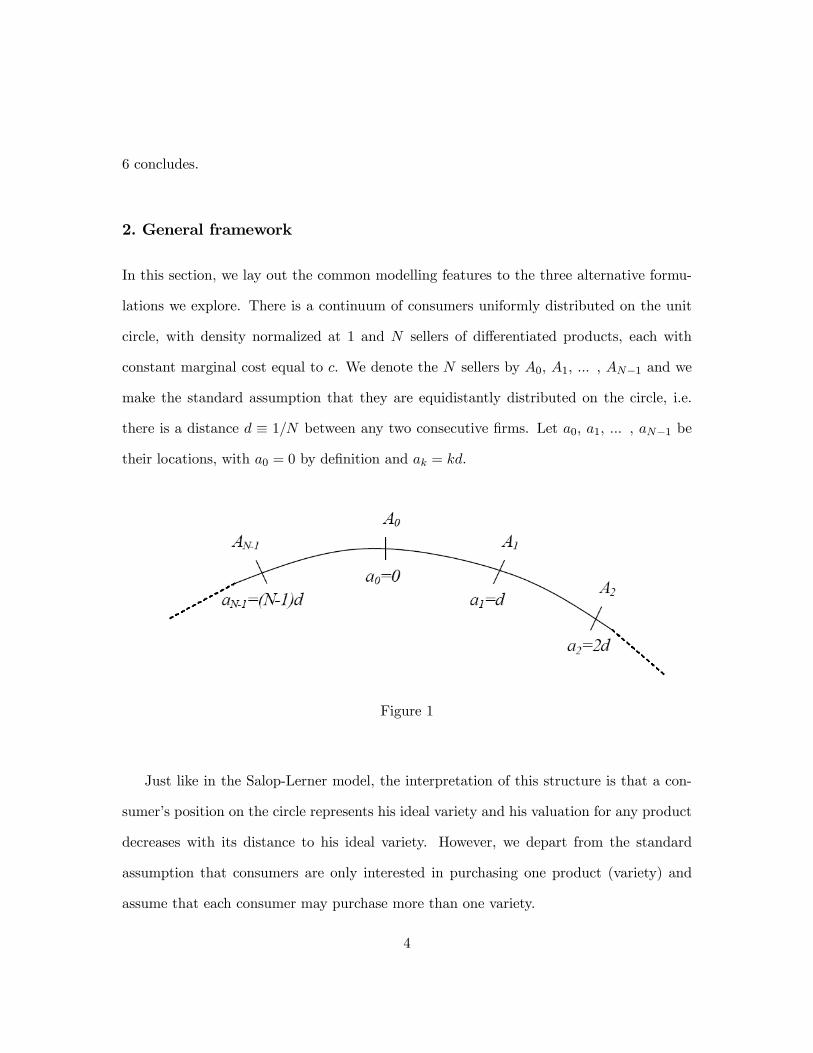
lations we explore. There is a continuum of consumers uniformly distributed on the unit

circle, with density normalized at 1 and N sellers of differentiated products, each with

constant marginal cost equal to c. We denote the N sellers by A0, A1, ... , AN−1 and we

make the standard assumption that they are equidistantly distributed on the circle, i.e.

there is a distance d ≡ 1/N between any two consecutive firms. Let a0, a1, ... , aN−1 be

their locations, with a0 = 0 by definition and ak = kd.

Figure 1

Just like in the Salop-Lerner model, the interpretation of this structure is that a con-

sumer’s position on the circle represents his ideal variety and his valuation for any product

decreases with its distance to his ideal variety. However, we depart from the standard

assumption that consumers are only interested in purchasing one product (variety) and

assume that each consumer may purchase more than one variety.

4

We take the equidistant location of firms as given (we are not interested in studying

differentiation incentives here). A simple way of justifying the assumption of equidistant

locations is to say that from the point of view of producers the location of any consumer’s

ideal product has equal chances of being anywhere on the circle.

The gross utility that any consumer derives from her ideal variety is v. In most of

the paper we deal with linear transportation costs. Thus, the net utility that a consumer

located at x on the circle derives from buying product Ai is given by:

u (x,Ai) = v − t |x− ai|− pai

where |a− b| stand for the distance between points a and b measured on the contour

of the circle.

This implies that, in ranking two products Ai and Aj , a consumer compares t |x− ai|+

pai with t |x− aj |+ paj .

Given that we think of "distances" in our model as distances in preference space rather

than in physical space (the latter being the common interpretation in spatial differentiation

models), it makes sense not to think of "transportation costs" literally. Consequently, t is

best interpreted as a taste parameter measuring how quickly the valuation of a consumer

for a variety falls with the "distance" to her ideal variety. In other words, t determines how

willing each consumer is to "explore" other varieties and thereby how many differentiated

products a consumer will end up purchasing.

In each of the three alternative formulations below, our goal will be to find a symmetric

price equilibrium, taking as given all the other parameters of the problem.

5

3. The case when demand is constrained by transportation costs

The first modelling option we explore is to let demand for differentiated products be con-

strained solely by the positive utility requirement. In other words, we allow each consumer

to buy all varieties which offer him non-negative utility, net of price and transportation

costs. Thus, the net utility of a consumer located at x on the circle is1:

U (x) =X

i∈{1,..N}v−t|x−aik |−pAi≥0

(v − t |x− ai|− pAi)

It is then clear that each firm has market power and since its demand and profits are

independent of the prices charged by and the number of other firms present in the market:

DAi (pAi) = 2(v − pAi)

t

ΠAi (pAi) = (pAi − c)DAi (pAi) =2 (pAi − c) (v − pAi)

t

Therefore, each firm’s profit-maximizing price and resulting profits are:

p (c) =v + c

2

Π (c) =(v − c)2

2t

With a more general expression of transportation costs, T (|x− ai|), T 0 > 0, we would

1Throughout the paper we assume that when a consumer is indifferent between buying and not buyinga variety, he will choose to buy.

6

obtain:

p (c) = argmaxp2 (p− c)D (p)

Π (c) = 2 (p (c)− c)D (p (c))

where D (p) ≡ T−1 (v − p)

The two expressions make clear that each firm acts like a monopoly. Moreover, note

that we would have obtained the same expressions (modulo a factor 2) if, rather than

starting with a circular distribution, we had assumed instead that consumers’ valuations

for each product were i.i.d. draws from the interval [0, v] according to a distribution

F (x) = 1− T−1 (v − x) = 1−D (x).

Lastly, we can determine consumer total and expected surplus2. They are given by:

Eu (N, c) = 2N

Z v−p(c)t

0(v − p (c)− tx) dx =

(v − p (c))2N

t

=(v − c)2N

4t

Using the generalized notation above, this expression becomes:

Eu (N, c) = N

Z v

p(c)D (x) dx

Overall, this case is not particularly interesting as all competition is removed when

consumers buy all products from which they derive non-negative utility. Thus, in order to

make our discussion interesting, we need to impose some kind of constraint on the number

of brands consumers can buy.

2They are equal because we normalized consumer mass to 1.

7

4. The number of varieties demanded is exogenously given

In the second formulation we introduce such a constraint by assuming that there is an

exogenously given number of varieties that consumers are interested in buying. Denote

this number by n, n < N . Then, a consumer located at x solves the following problem:

max{i1,i2,...,in}⊂{1,..N}

n³v − t |x− ai1 |− pAi1

´+ ...+

¡v − t |x− ain |− pAin

¢o

We also assume that v is large enough so that each consumer will in effect buy the n

varieties he prefers the most.

4.1. The case n = 2

We start by analyzing the case n = 2 in order to illustrate the basic mechanisms at work

in this case.

First, let us look for a candidate symmetric price equilibrium. In order to do so, suppose

all firms except one, say A0, charge the same price p, whereas A0 charges p0. Also, assume

p0 is close enough to p, more specifically:

¯̄p0 − p

¯̄< dt

This assumption ensures that there exists a unique location at which consumers are

indifferent between A0 and A1 and that it is strictly between a0 and a1 (and symmetrically

for AN−1 and A0). This location is given by:

x1 =d

2+

p− p0

2t

8

Similarly, consumers indifferent between A0 and A2 are located at:

x2 = d+p− p0

2t

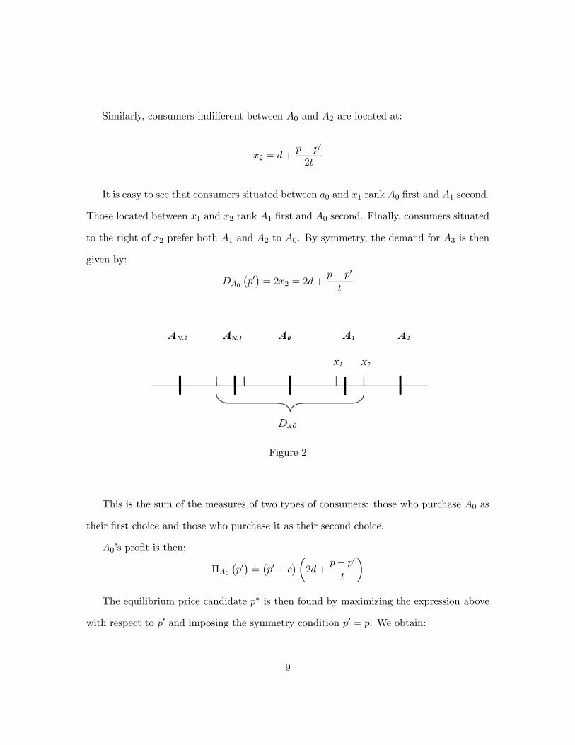
It is easy to see that consumers situated between a0 and x1 rank A0 first and A1 second.

Those located between x1 and x2 rank A1 first and A0 second. Finally, consumers situated

to the right of x2 prefer both A1 and A2 to A0. By symmetry, the demand for A3 is then

given by:

DA0

¡p0¢= 2x2 = 2d+

p− p0

t

Figure 2

This is the sum of the measures of two types of consumers: those who purchase A0 as

their first choice and those who purchase it as their second choice.

A0’s profit is then:

ΠA0¡p0¢=¡p0 − c

¢µ2d+

p− p0

t

¶The equilibrium price candidate p∗ is then found by maximizing the expression above

with respect to p0 and imposing the symmetry condition p0 = p. We obtain:

9

p∗ = c+ 2dt

At this price, all firms earn a profit of:

Π (p∗) = 4d2t

We now have to make sure that this price is indeed a Nash equilibrium, i.e. to check

whether there is no profitable deviation for A0, given that everyone else charges p∗. More

specifically we have to check whether there are no profitable deviations to p0 such that

|p0 − p∗| ≥ dt (we already know that p is better than any p0 such that |p0 − p∗| < dt).

It is precisely the feasibility of these larger deviations that makes the analysis here more

complex than the Salop model with demand for a single brand. Indeed, in that framework,

the candidate price equilibrium is c + dt and the non-existence of profitable deviations

larger than dt is immediate: undercutting by more than dt falls below cost and increasing

the price by at least dt clearly loses all demand.

In our case, the effect of introducing demand for more than one variety is to relax price

competition: equilibrium candidate prices are higher, which opens the possibility for more

numerous undercutting strategies, even though we will prove that they are not profitable

in the case n = 2.

If A0 charges p0 > p∗ + dt then demand for A0 will be 0: all consumers prefer at least

AN−1 and A1 over A0. Also, A0 has no interest in charging p0 ≤ p∗ − 2dt, since such a

price falls below cost.

Consider now the case p∗−2dt < p0 < p∗−dt, or c < p0 < c+dt. Clearly, all consumers

prefer A0 over A1. This is because the difference in prices between the two varieties is

too high in order to be compensated by any feasible difference in transportation costs.

10

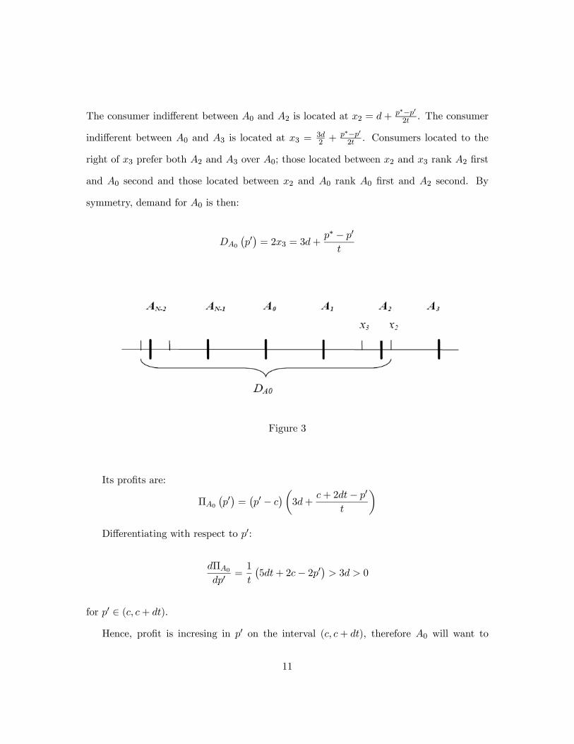
The consumer indifferent between A0 and A2 is located at x2 = d+ p∗−p02t . The consumer

indifferent between A0 and A3 is located at x3 = 3d2 +

p∗−p02t . Consumers located to the

right of x3 prefer both A2 and A3 over A0; those located between x2 and x3 rank A2 first

and A0 second and those located between x2 and A0 rank A0 first and A2 second. By

symmetry, demand for A0 is then:

DA0

¡p0¢= 2x3 = 3d+

p∗ − p0

t

Figure 3

Its profits are:

ΠA0¡p0¢=¡p0 − c

¢µ3d+

c+ 2dt− p0

t

¶Differentiating with respect to p0:

dΠA0dp0

=1

t

¡5dt+ 2c− 2p0

¢> 3d > 0

for p0 ∈ (c, c+ dt).

Hence, profit is incresing in p0 on the interval (c, c+ dt), therefore A0 will want to

11

charge p0 as close as possible to p∗ − dt = c+ dt:

limp0→p∗−dt,p0<p∗−dt

Π¡p0¢= 4d2t

and Π (p0) < 4d2t for p0 < p∗ − dt.

The reason we have to take a limit above is that demand is dicontinuous at p0 = p∗−dt.

Indeed, if A0 charges p0 = p∗ − dt, then all consumers to the right of A1 are indifferent

between A0 and A1. Consumers located between A0 and A1 rank A0 first and A1 second.

The rest is unchanged from the previous case. Hence, demand for A0 is now:

DA0 (p∗ − dt) = 2

µ3d

2+1

2× d

2

¶=7d

2

and its profit:

ΠA0 (p∗ − dt) =

7d2t

2< 4d2t

Lastly, assume A0 charges p0 = p∗ + dt. Consumers located to the right of A0 will be

indifferent between AN−1 and A0 and prefer A1 to both. The consumer indifferent between

A0 and A2 is located at d2 . Hence, demand and profit for A0 are:

DA0 (p∗ + dt) = 2× 1

2× d

2=

d

2

ΠA0 (p∗ + dt) =

3d2t

2< 4d2 /t

All these properties are illustrated in the following two diagrams, which represent the

demand and profit for A0 as functions of the price p0 it charges.

12

Figure 4

Figure 5

13

We have thus shown that there is no profitable deviation, which ensures that p∗ =

c+ 2dt is indeed a Nash equilibrium of the price game with differentiated products, when

consumers demand exactly 2 varieties. However, as we have seen and as is illustrated in

the second diagram above, this is "barely" an equilibrium, in the sense that there is an

undercutting strategy which does almost at least as well.

The next section proves the remarkable result that this strategy does strictly better

than the one prescribed by the candidate equilibrium and thus precludes the existence of

a symmetric equilibrium for n > 2.

4.2. The general case

Let now n be any integer strictly bigger than 1. The following proposition contains the

central result of this section.

Proposition 1. With linear transportation costs and equidistant locations, there is no

symmetric price equilibrium if the number of varieties demanded by consumers is strictly

higher than 2.

Proof. The determination of the candidate price equilibrium follows the same lines as

above and is straightforward. Suppose everyone charges p, except A0, who charges p0, with

|p0 − p| < dt. For every Ak with k > 0, the consumer indifferent between A0 and Ak exists

and is located at:

xk =kd

2+

p− p0

2t

It is easy to see that consumers located between xk and xk+1 rank A0 in (k + 1) th

position. Therefore, the last consumer to the right of A0 who will buy variety A0 is the

14

one located at xn. Demand for A0 is then:

DA0

¡p0¢= 2

µnd

2+

p− p0

2t

¶

The following diagram illustrates the case n = 4.

Figure 6

Maximizing profit and imposing that the solution be equal to p yields:

p∗n = ndt+ c

At this price, each seller has a market share of:

x∗n = nd

and makes a profit of:

Π (p∗n) = n2d2t

The range of potentially profitable deviations is¡−ndt,+E

¡n2

¢dt¤. Indeed, if A0

charges more than p∗n + E¡n2

¢dt, even the consumer located exactly at a0 will rank A0

15

in¡2E¡n2

¢+ 1¢th position and will not buy it since 2E

¡n2

¢+ 1 ≥ n + 1 > n. Since this

consumer is the most likely to buy A0, demand for A0 will be 0.

However, we will prove that undercutting strategies at non-discontinuous points are

enough to eliminate the symmetric price equilibrium candidate.

Assume that:

p0 ∈ (p∗n − (k + 1) dt, p∗n − kdt) , for some k ∈ [1, n− 1]

When A0 charges such a price, all consumers rank A0 before A1, A2, .., Ak and the first

variety to the right of A0 for which there exist some consumers that prefer it to A0 is Ak+1.

The last consumer to the right of A0 who will purchase A0 is then the one who is indifferent

between A0 and Ak+n, located at xk+n =(k+n)d2 + p∗n−p0

2t . The following diagram illustrates

this for n = 4 and k = 2:

Figure 7

16

Demand and profits for A0 are then:

DA0

¡p0¢= 2xk+n = (k + n) d+

p∗n − p0

t

ΠA0¡p0¢=

¡p0 − c

¢µ(k + n) d+

p∗n − p0

t

¶

Differentiating with respect to p0 and using the fact that p0 ∈ (c+ (n− (k + 1)) dt, c+ (n− k) dt),

we obtain:

dΠA0dp0

=1

t

¡(k + 2n) dt+ 2c− 2p0

¢>

1

t((k + 2n) dt+ 2c− 2 (c+ (n− k) dt))

= 3kd > 0

Hence profit is increasing on each interval (c+ (n− (k + 1)) dt, c+ (n− k) dt) and:

limp0→(p∗−kdt)−

ΠA0¡p0¢= (n− k) (2k + n) d2t =

¡n2 + kn− 2k2

¢d2t

Taking k = 1, the limit above is equal to:

¡n2 + n− 2

¢d2t > n2d2t = Π (p∗n) for n ≥ 3

This means that for n ≥ 3, there always exists a profitable undercutting strategy (any

price inferior but close enough to p∗ − kdt will do) and thus there is no symmetric price

equilibrium. This concludes the proof.

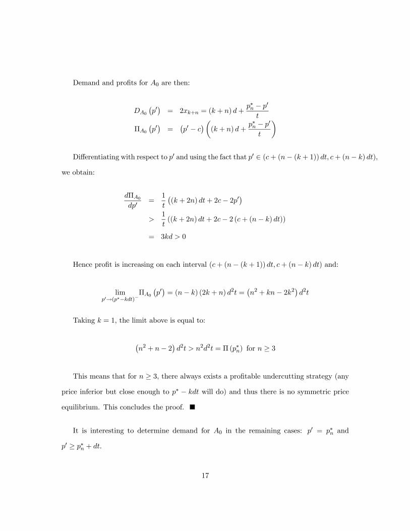
It is interesting to determine demand for A0 in the remaining cases: p0 = p∗n and

p0 ≥ p∗n + dt.

17

Let p0 = p∗n − kdt, for some k ∈ [1, n]. It is straightforward to prove (same as in the

case n = 2):

DA0

¡p0¢= 2

µxn+k−1 +

1

2(xn+k − xn+k−1)

¶=

µn+ 2k − 1

2

¶d

ΠA0¡p0¢= (n− k)

µn+ 2k − 1

2

¶d2t

=

µn2 +

µk − 1

2

¶n− k

µ2k − 1

2

¶¶d2t <

¡n2 + kn− 2k2

¢d2t

Next, let p0 ∈ (p∗n + kdt, p∗n + (k + 1) dt) = (c+ (n+ k) dt, c+ (n+ k + 1) dt). Then,

the consumer located at x = a0 ranksA0 in position 2k+1, i.e. afterAN−k, ..., AN−1, A1, ..., Ak.

The last consumer to the right of A0 who will purhcase A0 will be the one indifferent be-

tween A0 and An−k. Therefore, demand and profits for A0 are:

DA0

¡p0¢= 2× xn−k = (n− k) d+

p∗n − p0

t

ΠA0¡p0¢=

¡p0 − c

¢µ(n− k) d+

p∗n − p0

t

¶

And:

dΠA0dp0

=1

t

¡(2n− k) dt+ 2c− 2p0

¢<

1

t((2n− k) dt+ 2c− 2 (c+ (n+ k) dt))

= −3kd < 0

18

Hence profit is decreasing on each interval (c+ (n+ k) dt, c+ (n+ k + 1) dt) and:

limp0→(p∗+kdt)+

ΠA0¡p0¢= (n+ k) (n− 2k) d2t

=¡n2 − kn− 2k2

¢d2t < n2d2t

Lastly, for p0 = p∗ + kdt, k ≥ 1:

DA0

¡p0¢= xn−k +

1

2(xn−k+1 − xn−k) =

µn− 2k + 1

2

¶d

ΠA0¡p0¢= (n+ k)

µn− 2k + 1

2

¶d2t

=

µn2 −

µk − 1

2

¶n− k

µ2k − 1

2

¶¶d2t < n2d2t

Thus, no deviation p0 > p∗ + dt is profitable.

The following diagrams show demand and profits for A0 as a function of its price p0 for

n = 4.

19

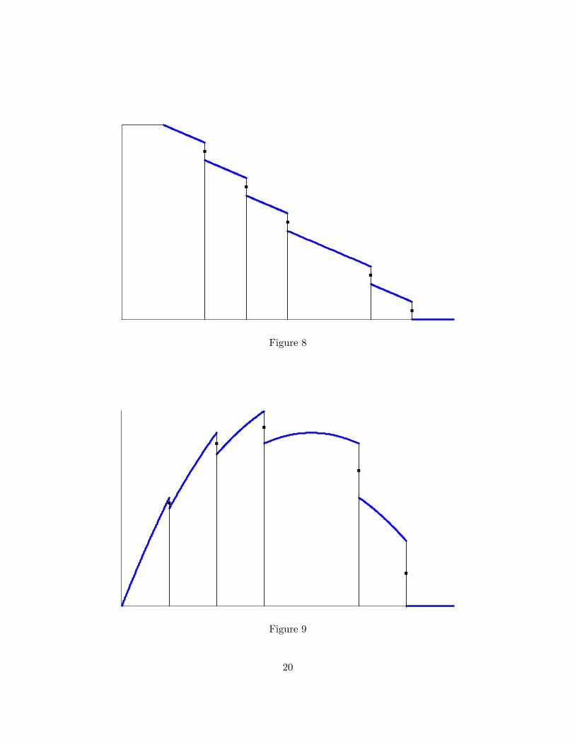
Figure 8

Figure 9

20

The two diagrams show that the possibility of a profitable deviation arises because

demand jumps up sharply at every threshold of the form p∗n− kdt for k ≥ 1. This happens

because each time A0’s price p0 falls below such a threshold, it "completely" undercuts

firm Ak, meaning that the price difference is enough so that no consumer will ever prefer

Ak over A0. This instantly pushes demand up by d. It is important to note that these

marginal consumers of mass d that A0 gains are those furthest away from A0, i.e. those

whose "last" (nth) purchase (in terms of distance travelled) right before the threshold was

Ak. Once p0 falls below p∗n− kdt though, it becomes worthwhile for them to forego Ak and

travel the extra distance in order to get A0. Note that the reason they do not stop on their

way from Ak to A0 to any of the shops in between (Ai with 1 ≤ i ≤ k − 1) is because A0

was already worth travelling the extra mile conditional on one having decided to venture

past Ak in the direction of A0.

Hence, at threshold k, A0’s profit jumps up by (p∗n − kdt− c) d = (n− k) d2t. Clearly,

this jump is highest for k = 1. However, it is not true that the optimal undercutting

strategy is near p∗n−dt. To see this, note that profits fall by (3k + 1) d2t when A0 decreases

its price from threshold k to threshold k + 1, therefore, as long as this is less than what it

stands to gain through the jump at threshold k+1, A0 has every interest in cutting its price

further. It will stop when the size of the next jump is no longer worth the loss incurred

through the discrete decrease in price needed in order to get to the next threshold. The

marginal condition is thus 3k+1 ≥ n− (k + 1) or 4k+2 ≥ n, which is almost the same as

the first order condition obtained by maximizing the limit deviation profit at threshold k

with respect to k: k = n4 . The difference is simply due to integer problems. In our diagram

above, the optimal deviation is at the threshold k = 1 because n = 4. It will be that way

for n ≤ 6; for n = 7 for example, the optimal deviation is p∗n − 2dt.

21

Given the negative result above, one might hope that it is due to the specificity of

linear transportation costs, which yield, as is well-known and as we have shown above,

discontinuous demand functions. It turns out that the non-existence of a symmetric price

equilibrium persists even with strictly convex transportation costs, i.e. tdβ with β > 1, as

shown by the theorem below, which we prove in the appendix.

Proposition 2. If consumers are interested in buying exactly n varieties and transporta-

tion costs are convex, i.e. of the form tdβ with β > 1, then there exists−n (β) such that, if

N > n ≥ −n (β), then there is no symmetric price equilibrium with N equidistantly located

firms.

Proof. See appendix.

The two figures below illustrate this result for β = 2 and n = 4. Both demand and

profits for A0 are continuous in p0, however their derivatives are discontinuous, which

explains the existence of profitable undercutting strategies (the graphs are drawn only for

p0 ≤ p∗ (n) + tdβ).

22

Figure 10

Figure 11

23

Note that it may well be that there is no symmetric price equilibrium even for n <−n (β).

However, in order to prove or disprove this one would have to go through some serious

algebra. Our goal was to find a price equilibrium for general n and the propositions above

proved that this is impossible. For example, it is straightforward to show that−n (2) = 4,

meaning that with quadratic transportation costs there is no symmetric price equilibrium

for n ≥ 4. Therefore, our non existance result is quite robust when we generalize to

non-linear transportation costs.

5. The case when consumers face a budget constraint

In the third and last alternative we explore, we assume that the restriction on the number

of products that every consumer purchases comes from a budget constraint, rather than

from an exogenous limit on the number of varieties purchased like in the previous section.

More specifically, we assume that each consumer has a limited budget I: he will purchase

varieties by decreasing order of preference, and will stop when the sum of the prices he has

paid exceeds I.

Hence, a consumer located at x on the circle solves the following problem:

U (x) = maxk∈[1,N ]

{i1,i2,...,ik}⊂{1,..N}pAi1

+...+pAik≤I

n(v − t |x− ai1 |) + ...+ (v − t |x− aik |) + I − pAi1

− ...− pAik

o

It is important to note that here consumers choose not only which varieties to buy, but

also how many, as long as they respect the budget constraint. In other words, k in the

maximization program above is a choice variable, whereas in our previous model we had

imposed an exogenous limit on the number of varieties demanded by consumers, i.e. k was

given.

24

The following proposition characterizes all possible symmetric price equilibria.

Proposition 3. Assume v ≥ max¡t2 + 2dt+ c, I2 + t

¢. Then there are only two possible

types of equilibria:

• If I can be written as I = k (c+ kdt)+x, where 0 ≤ x < c+kdt and k ∈ {1, 2}, then

p = c+kdt is a symmetric price equilibrium if and only if x < max¡c, k2d2t

¢. In this

equilibrium, each consumer purchases 2 varieties.

• For all integer n ∈£a,min

¡Ic , N

¢¤, where a is the unique positive solution to I

a =

c+¡a2 + 1

¢dt, there exists a symmetric price equilibrium with p = I

n , in which each

consumers buys n varieties.

Proof. Consider a symmetric price equilibrium candidate p. Let n = E³Ip

´and write:

I = np+ x, where 0 ≤ x < p

In order to characterize p, we assume throughout the proof that all firms charge p, with

the exception of A0, which charges p0.

Let xk be the location of the consumer indifferent between A0 and Ak, irrespective of

budget considerations:

xk =kd

2+

p− p0

2t, for k ≥ 1

Clearly, xk exists if and only if |p− p0| < kdt.

The following lemma gives a partial (but sufficient for our purposes) characterization

of the demand for A0:

Lemma 1. Assume x < p0 ≤ p+ x throughout.

25

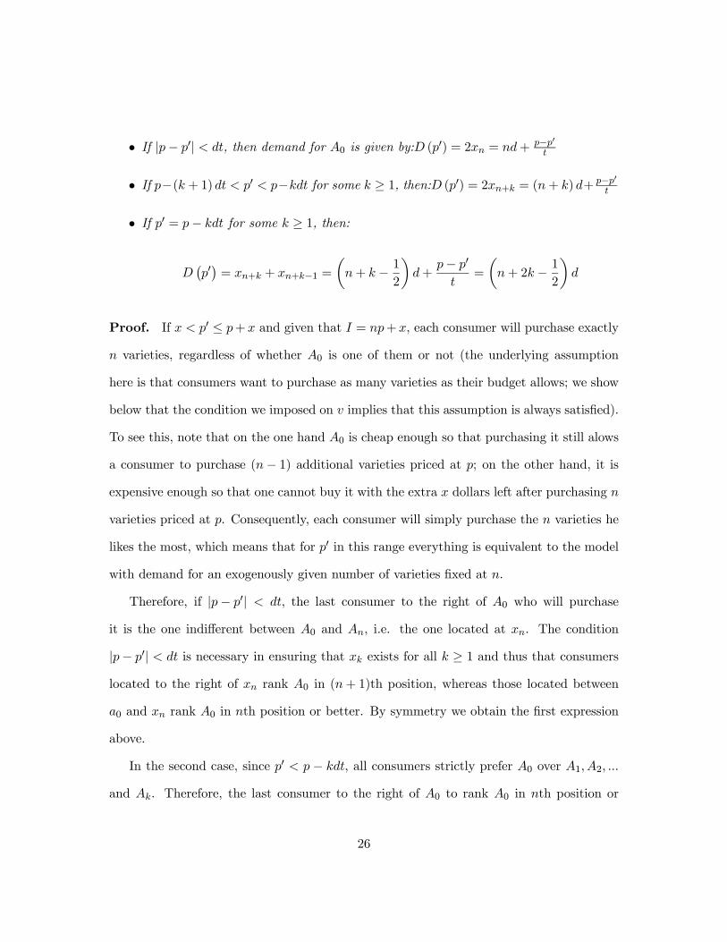
• If |p− p0| < dt, then demand for A0 is given by:D (p0) = 2xn = nd+ p−p0t

• If p−(k + 1) dt < p0 < p−kdt for some k ≥ 1, then:D (p0) = 2xn+k = (n+ k) d+ p−p0t

• If p0 = p− kdt for some k ≥ 1, then:

D¡p0¢= xn+k + xn+k−1 =

µn+ k − 1

2

¶d+

p− p0

t=

µn+ 2k − 1

2

¶d

Proof. If x < p0 ≤ p+ x and given that I = np+ x, each consumer will purchase exactly

n varieties, regardless of whether A0 is one of them or not (the underlying assumption

here is that consumers want to purchase as many varieties as their budget allows; we show

below that the condition we imposed on v implies that this assumption is always satisfied).

To see this, note that on the one hand A0 is cheap enough so that purchasing it still alows

a consumer to purchase (n− 1) additional varieties priced at p; on the other hand, it is

expensive enough so that one cannot buy it with the extra x dollars left after purchasing n

varieties priced at p. Consequently, each consumer will simply purchase the n varieties he

likes the most, which means that for p0 in this range everything is equivalent to the model

with demand for an exogenously given number of varieties fixed at n.

Therefore, if |p− p0| < dt, the last consumer to the right of A0 who will purchase

it is the one indifferent between A0 and An, i.e. the one located at xn. The condition

|p− p0| < dt is necessary in ensuring that xk exists for all k ≥ 1 and thus that consumers

located to the right of xn rank A0 in (n+ 1)th position, whereas those located between

a0 and xn rank A0 in nth position or better. By symmetry we obtain the first expression

above.

In the second case, since p0 < p − kdt, all consumers strictly prefer A0 over A1, A2, ...

and Ak. Therefore, the last consumer to the right of A0 to rank A0 in nth position or

26

better is now located at xn+k instead of xk.

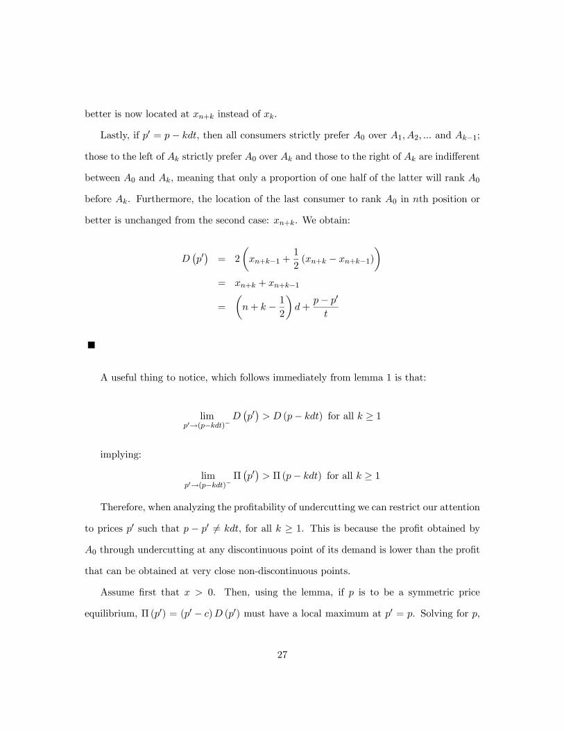
Lastly, if p0 = p − kdt, then all consumers strictly prefer A0 over A1, A2, ... and Ak−1;

those to the left of Ak strictly prefer A0 over Ak and those to the right of Ak are indifferent

between A0 and Ak, meaning that only a proportion of one half of the latter will rank A0

before Ak. Furthermore, the location of the last consumer to rank A0 in nth position or

better is unchanged from the second case: xn+k. We obtain:

D¡p0¢= 2

µxn+k−1 +

1

2(xn+k − xn+k−1)

¶= xn+k + xn+k−1

=

µn+ k − 1

2

¶d+

p− p0

t

A useful thing to notice, which follows immediately from lemma 1 is that:

limp0→(p−kdt)−

D¡p0¢> D (p− kdt) for all k ≥ 1

implying:

limp0→(p−kdt)−

Π¡p0¢> Π (p− kdt) for all k ≥ 1

Therefore, when analyzing the profitability of undercutting we can restrict our attention

to prices p0 such that p − p0 6= kdt, for all k ≥ 1. This is because the profit obtained by

A0 through undercutting at any discontinuous point of its demand is lower than the profit

that can be obtained at very close non-discontinuous points.

Assume first that x > 0. Then, using the lemma, if p is to be a symmetric price

equilibrium, Π (p0) = (p0 − c)D (p0) must have a local maximum at p0 = p. Solving for p,

27

this yields:

p = c+ ndt

This cannot be an equilibrium if n > 2. Indeed, just like in the model where n is

exogenously given, there exist profitable undercutting strategies. For example, A0 can

charge p0 = p− dt− dt = c+ (n− 1) dt− dt, with very small, for a profit equal to:

Π¡p0¢= ((n− 1)− ) ((n+ 2) + ) d2t > n2d2t = Π (p) for n > 2

Therefore we must have n ≤ 2. We still have to check under what conditions there are

no profitable deviations.

For p0 > p+dt, AN−1 and A1 are always strictly preferred to A0, hence the latter makes

no sales and therefore such a deviation cannot be profitable.

If n = 1, charging p0 > p + x = I yields 0 sales, hence cannot be profitable. If n = 2,

p0 > p+x makes no sales either. To see this, note that any consumer buying A0 cannot buy

anything else, whereas otherwise he can buy 2 varieties. Consider the consumer located at

a0. He has the choice between purchasing A0 or purchasing AN−1 and A1. He will choose

the latter option if and only if:

2v − 2p− 2dt ≥ v − p0

⇐⇒ v ≥ 2p− p0 + 2dt

But

2p− p0 + 2dt < p+ 2dt ≤ I

2+2

Nt ≤ I

2+ t ≤ v by assumption

Therefore, since not even the consumer whose ideal variety is A0 will not purchase it,

28

demand for A0 is 0 in this case as well.

The only possible deviation we are left with is p0 ≤ x. If x ≤ c, this cannot be

profitable. If x > c, such a price ensures that all consumers who derive positive utility

from the purchase of A0 will buy it, since it is the only additional variety that can be

bought after purchasing n varieties at price p (recall that I = np+ x). Hence:

D¡p0¢= min

µ2 (v − p0)

t, 1

¶= 1

because 2(v−p0)t > 2(v−p)

t ≥ 2(v−c−2dt)t ≥ 1

The maximum profit that A0 can get with such a deviation is then x. This deviation

is not profitable if and only if:

x < max¡c, n2d2t

¢We have thus proven that a symmetric price equilibrium p such that I = np+ x with

0 < x < p can only exist for n ≤ 2 and p = c+ ndt.

Let us now look for symmetric price equilibria such that I = np. Lemma 1 still applies

for p0 ≤ p (with x = 0). However, the important thing to notice is that now p0 = p does not

necessarily have to be a local maximum for Π (p0) = (p0 − c)³nd+ p−p0

t

´. Indeed, lemma

2 below shows that under our assumptions on v, demand for A0 is 0 for p0 > p.

Lemma 2. If A0 charges p0 while all other firms charge p = In , with p

0 > p and if v ≥ I2+t,

then A0 makes 0 sales.

Proof. If a consumer does not purchase A0 then she can purchase n total varieties,

whereas if she does, she can only purchase n − 1 total varieties. Consider a consumer

located at a0+ , with > 0 small. Assume n = 2k. She has the choice between purchasing

29

A0, A1,...,Ak−1, AN−1, AN−2,..., AN−k+1 or A1,...,Ak, AN−1, AN−2,..., AN−k and she

prefers the latter if and only if:

2v − 2p− t | − ak|− t | − aN−k| ≥ v − p0

v − 2p+ p0 − 2kdt ≥ 0

v − 2p+ p0 − ndt ≥ 0

One can easily show that this condition is valid for n = 2k + 1 as well.

We have:

v − 2p+ p0 − ndt > v − p− ndt = v − I

n− n

Nt > v − I − t ≥ 0

Thus for any small no consumer located at a0 + will purchase A0. Since these are

the consumers who like A0 the most, it is clear that a fortiori no other consumers to the

right of A0 will purchase it. The same is true by symmetry for consumers to the left of A0,

which completes the proof of the lemma.

The result proven in lemma 2 is the crucial difference between the model with demand

for an exogenously given number of varieties and the present model with a budget con-

straint. It is the reason why there exists a symmetric equilibrium in the latter as opposed

to the former. Indeed, by assuming that v is large enough, we made sure that a consumer

would forego even her ideal variety if she can purchase two varieties instead. This tradeoff

is relevant when the budget constraint is binding and the price of the ideal variety is strictly

higher than the price of all other varieties. Consequently, since raising p0 ever so slightly

over p yields 0 profits (this discontinuity in the profit function is entirely due to the budget

30

constraint), we simply have to make sure that:

Π¡p0¢≤ Π (p) = (p− c)nd for all p0 ≤ p

if we want p to be a symmetric price equilibrium immune to undercutting strategies. By

contrast, in the previous model p had to be a local maximum for Π (.) (i.e. dΠ(p0)dp0 (p0 = p) =

0), which imposed too high a symmetric price equilibrium candidate.

Given our remark after lemma 1, the necessary and sufficient conditions here are:

dΠ (p0)

dp0¡p0 = p

¢≥ 0

and for all k ≥ 1, supp0∈(p−(k+1)dt,p−kdt)

Π¡p0¢≤ Π (p)

The first condition is equivalent to:

p ≤ c+ ndt

For simplicity, write:

p = c+ ydt, with y ∈ [0, n]

Then:

Π (p) = ynd2t

31

For p0 ∈ (p− (k + 1) dt, p− kdt), we have:

dΠ (p0)

dp0= (n+ k) d+

p− p0

t− p0 − c

t

=c+ (n+ k) dt+ p− 2p0

t

>c+ (n+ k) dt− p+ 2kt

t> 0

Thus:

supp0∈(p−(k+1)dt,p−kdt)

Π¡p0¢= lim

p0→(p−kdt)−Π¡p0¢= (p− kdt− c) (n+ 2k) d

= (y − k) (n+ 2k) d2t

The second condition above is then satisfied if and only if (y − k) (n+ 2k) ≤ yn for any

integer k ∈ [1, y], or 2k¡y − k − n

2

¢≤ 0 for any integer k ∈ [1, y]. This is satisfied if and

only if y − 1− n2 ≤ 0 or y ≤

n2 + 1.

We have thus shown that p = In is a symmetric price equilibrium if and only if:

p ≤ c+³n2+ 1´dt

⇐⇒ I

n≤ c+

³n2+ 1´dt

⇐⇒ n ≥ a

where a is the unique positive solution to:

I

a= c+

³a2+ 1´dt

32

Lastly, we have to make sure the interval£a,min

¡Ic , N

¢¤is not empty:

I

(I/c)= c < c+

µI

2c+ 1

¶dt =⇒ a <

I

c

and:

N ≥ a⇐⇒ I − t

N≤ c+

t

2

Thus, for N large enough, the interval above is well-defined. If N is such that the

second inequality above does not hold, then there is no symmetric price equilibrium of the

second type.

This completes the proof of the proposition.

Clearly, the conditions for existence of the first type of equilibria (there are at most

2, one with n = 1 and one with n = 2) are quite restrictive and these equilibria will not

exist in general. It is the existence of the second type of equilibria which is interesting and

which stands in stark contrast with the non-existence result we obtained in the previous

section, with demand for an exogenously given number of varities.

The figures below depict demand and profits around such an equilibrium, with N = 10,

c = 1, t = 10, n = 4 and I = 15 (a = 3.83).

33

Figure 12

Figure 13

34

5.1. Welfare analysis

The welfare analysis here (in particular the comparison of the socially optimal number of

firms and the one occuring with free entry) is quite different from the Lerner Salop model

for two reasons. First, for any given number of firms active in the market there are multiple

symmetric equilibria and it is not clear which will occur when an additional firm enters

the market. Secondly, before determining the socially optimal number of firms, we need to

rank the multiple equilibria that can occur for any given number of active firms.

For any given N , let us index each possible equilibrium that may occur by n, the

number of products that consumers buy in that equilibrium. As we have seen above, n lies

in the interval£a,min

¡Ic , N

¢¤. The corresponding symmetric price equilibrium is:

pn =I

n

With free entry, the profit for each firm as a function of n and N is:

π (N,n) =

µI

n− c

¶nd− f =

I − cn

N− f

This expression captures the difficulty of analyzing free entry in our context. Indeed,

assume as is standard that the zero profit condition holds for n > 1. If a potential entrant

believes that in case she enters firms will coordinate on an equilibrium n0 with n0 ≥ n,

then entry is not profitable. However, if she expects firms to coordinate on any equilibrium

n0 < n, entry may be profitable. More precisely, this happens if and only if:

I − cn0

N + 1>

I − cn

N

35

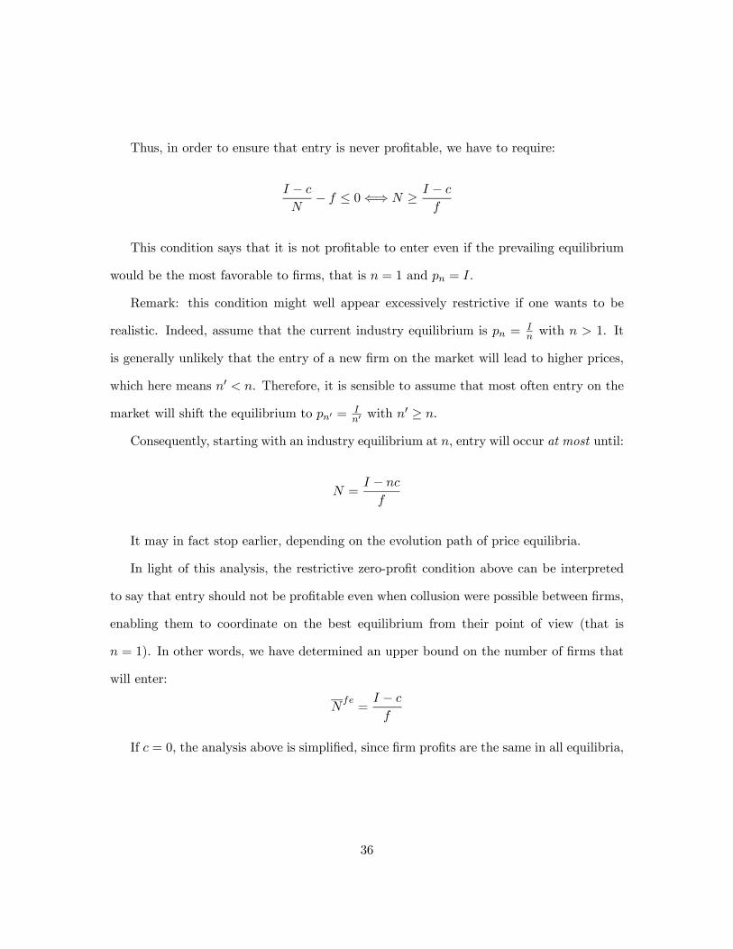
Thus, in order to ensure that entry is never profitable, we have to require:

I − c

N− f ≤ 0⇐⇒ N ≥ I − c

f

This condition says that it is not profitable to enter even if the prevailing equilibrium

would be the most favorable to firms, that is n = 1 and pn = I.

Remark: this condition might well appear excessively restrictive if one wants to be

realistic. Indeed, assume that the current industry equilibrium is pn = In with n > 1. It

is generally unlikely that the entry of a new firm on the market will lead to higher prices,

which here means n0 < n. Therefore, it is sensible to assume that most often entry on the

market will shift the equilibrium to pn0 = In0 with n0 ≥ n.

Consequently, starting with an industry equilibrium at n, entry will occur at most until:

N =I − nc

f

It may in fact stop earlier, depending on the evolution path of price equilibria.

In light of this analysis, the restrictive zero-profit condition above can be interpreted

to say that entry should not be profitable even when collusion were possible between firms,

enabling them to coordinate on the best equilibrium from their point of view (that is

n = 1). In other words, we have determined an upper bound on the number of firms that

will enter:

Nfe=

I − c

f

If c = 0, the analysis above is simplified, since firm profits are the same in all equilibria,

36

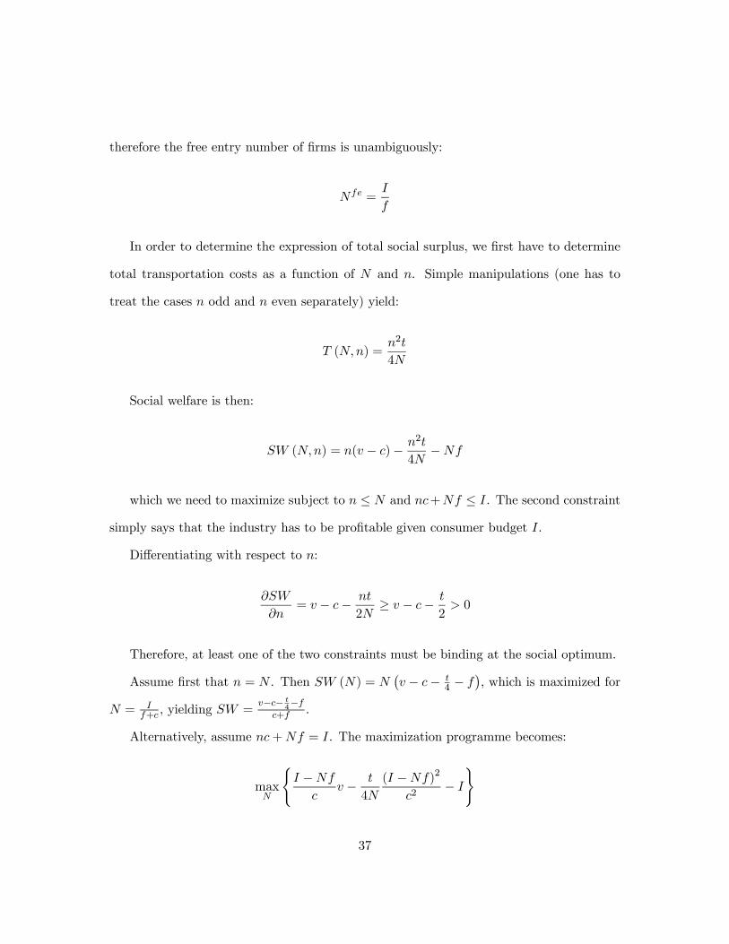
therefore the free entry number of firms is unambiguously:

Nfe =I

f

In order to determine the expression of total social surplus, we first have to determine

total transportation costs as a function of N and n. Simple manipulations (one has to

treat the cases n odd and n even separately) yield:

T (N,n) =n2t

4N

Social welfare is then:

SW (N,n) = n(v − c)− n2t

4N−Nf

which we need to maximize subject to n ≤ N and nc+Nf ≤ I. The second constraint

simply says that the industry has to be profitable given consumer budget I.

Differentiating with respect to n:

∂SW

∂n= v − c− nt

2N≥ v − c− t

2> 0

Therefore, at least one of the two constraints must be binding at the social optimum.

Assume first that n = N . Then SW (N) = N¡v − c− t

4 − f¢, which is maximized for

N = If+c , yielding SW =

v−c− t4−f

c+f .

Alternatively, assume nc+Nf = I. The maximization programme becomes:

maxN

(I −Nf

cv − t

4N

(I −Nf)2

c2− I

)

37

subject to N ≥ If+c .

Straightforward calculations show that the expression above is decreasing in N for

N ≥ If+c (we also use the assumption v > t

2 and the natural c ≤ f):

f (N) =I −Nf

cv − t

4N

(I −Nf)2

c2− I

f 0 (N) = −vfc+

tI

4c2N2(I − fN)

≤ −vfc+

tI

4cN=

1

cN

µtI

4−Nvf

¶≤ I

cN

µt

4− vf

f + c

¶≤ 0

Thus the solution is once again n = N = If+c .

The social optimum is characterized by:

nso = Nso =I

c+ f

In the general case when c > 0, the socially optimum level of entry is higher than the

maximum number of firms under free entry if and only if:

I

c+ f≥ I − c

f⇐⇒ I ≤ f + c

Thus, free entry always leads to a suboptimal number of firms on the market if this condi-

tion is satisfied. Otherwise this number may be exactly optimal, suboptimal or excessive,

depending on the price equilibria that prevail.

38

6. Conclusion

This paper has proposed a theoretical framework for studying competition between dif-

ferentiated products, when consumers are interested in purchasing more than one brand.

Indeed, the two classic frameworks for studying monopolistic competition - based on Salop

(1979) and, respectively, on Spence (1976) and Dixit and Stiglitz (1977) - do not seem ad-

equate proxies for markets such as those for software applications and videogames, which

combine features of both models, most importantly product differentiation, heterogeneity of

consumer tastes and consumer preference for diversity. Accordingly, our model generalizes

Salop’s circular framework by allowing consumers to purchase more than one variety.

The case in which consumers buy all products offering net positive utility is not very

interesting, as there is no competition among firms, so that each behaves like an uncon-

strained monopolist. Therefore the need to place a restriction on the number of varieties

consumers purchase. The surprising result is that when each consumer demands an exoge-

nously fixed number of varieties, a pure strategy symmetric price equilibrium does not exist

in general. This is because of two conflicting effects: on the one hand, when consumers

buy more products, competition is relaxed so that first order conditions for maximization

entail higher prices. But on the other hand higher prices open up the possibility for very

aggressive undercutting strategies, which achieve de facto vertical differentiation from rivals

offering similar products and thus discrete increases in market shares and profits. By con-

trast, if we assume instead that the number of varieties consumers purchase is indirectly

limited by a budget constraint, then we obtain multiple pure strategy symmetric price

equilibria, each corresponding to a different number of varieties bought by consumers. The

reason is that in this case the budget constraint eliminates the need for local first order

maximization, allowing prices to be lower and therefore immune to the previously described

39

aggressive undercutting strategies.

7. APPENDIX

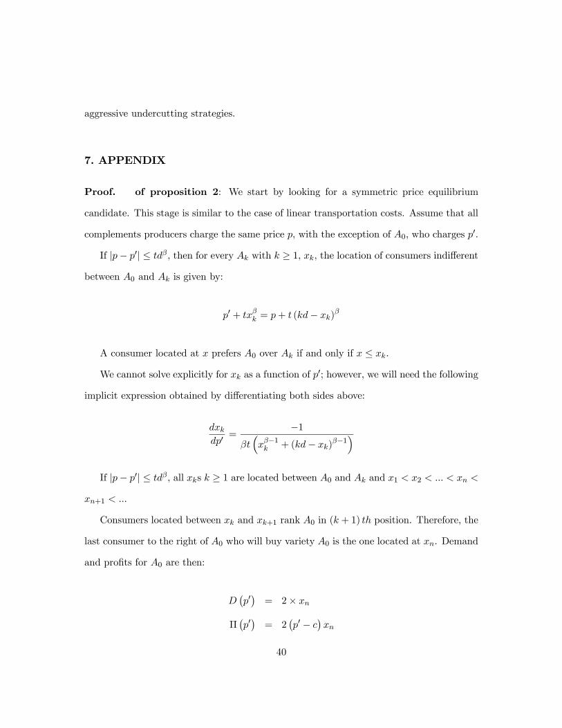
Proof. of proposition 2: We start by looking for a symmetric price equilibrium

candidate. This stage is similar to the case of linear transportation costs. Assume that all

complements producers charge the same price p, with the exception of A0, who charges p0.

If |p− p0| ≤ tdβ, then for every Ak with k ≥ 1, xk, the location of consumers indifferent

between A0 and Ak is given by:

p0 + txβk = p+ t (kd− xk)β

A consumer located at x prefers A0 over Ak if and only if x ≤ xk.

We cannot solve explicitly for xk as a function of p0; however, we will need the following

implicit expression obtained by differentiating both sides above:

dxkdp0

=−1

βt³xβ−1k + (kd− xk)

β−1´

If |p− p0| ≤ tdβ, all xks k ≥ 1 are located between A0 and Ak and x1 < x2 < ... < xn <

xn+1 < ...

Consumers located between xk and xk+1 rank A0 in (k + 1) th position. Therefore, the

last consumer to the right of A0 who will buy variety A0 is the one located at xn. Demand

and profits for A0 are then:

D¡p0¢= 2× xn

Π¡p0¢= 2

¡p0 − c

¢xn

40

Next, we differentiateΠwith respect to p0 using [] above and we impose that dΠdp0 (p

0 = p) =

0, which, given convex transportation costs ensures that p0 = p maximizes Π locally.

Straightforward calculations yield the following characterization of the symmetric price

equilibrium candidate:

p∗ (n) = c+ 21−βtβ (nd)β

D (p∗ (n)) = nd

Π (p∗ (n)) = 21−βtβ (nd)β+1

We will now prove that we can find−n (β) such that for n ≥ −

n (β), there always exist

profitable undercutting strategies for A0.

For simplification purposes, let:

δ =p∗ (n)− p0

t≥ 0

We have to determine demand for A0 as a function of δ. Like in the case with linear

transportation costs, this depends on the positions of the xis. The main difference with

strictly convex transportation costs is that now xi exists for all i and for all δ. However,

their relative positions change with δ as we show below.

Denote by k (δ) the unique, non negative integer such that:

δ ∈h(k (δ) d)β , ((k (δ) + 1) d)β

´

Then:

41

• if i ≤ k (δ), then xi uniquely solves:

xβi − (xi − id)β = δ

and xi ≥ id

• if i ≥ k (δ) + 1, xi uniquely solves:

xβi − (id− xi)β = δ

and xi < id

It is easily seen that xi (δ) is continuous and strictly increasing in δ for all i and that:

x1 (δ) > x2 (δ) > ... > xk(δ) (δ) ≥ k (δ) d

xk(δ)+1 (δ) < xk(δ)+2 (δ) < ... < xk(δ)+l (δ) < ...

Now, for any i > j, denote by δij the unique value of δ such that xi(δ) = xj (δ) and let

xij = xi(δij) = xj(δij). Given the strict inequalities above, it is clear that one must have:

i > k (δij) ≥ j

δij ∈h(jd)β , (id)β

´

Simple calculations yield:

xij =(i+ j) d

2

δij =

µd

2

¶β ³(i+ j)β − (i− j)β

´42

Clearly, δij is increasing in both i and j. Also, one has the following additional property:

xi (δ) ≥ xj (δ)⇐⇒ δ ≤ δij

We are now in a position to determine the demand for A0 when it charges p0 and

everyone else charges p, i.e. when it chooses to undercut by δ.

Consumers will purchase A0 if and only if they rank it in nth position or better. This

means that a consumer to the right of A0 will purchase it if and only if there are at most

(n− 1) xi’s between this consumer’s position and A0. Hence, by symmetry, demand for

A0 is exactly equal to twice the nth xi, when one orders them by increasing value. All

the difficulty in this case consists in determining which xi is number n; indeed, once δ is

greater than δn1 it is no longer xn.

The following lemma characterizes demand for A0 as a function of δ for δ ≥ 0:

Lemma 3. For all k ≥ 1:

• If δ ∈ [0, δn1], then DA0 (δ) = 2xn

• if δ ∈£δ(n+k−1)k, δ(n+k)k

¢then DA0 (δ) = 2xk

• if δ ∈£δ(n+k)k, δ(n+k)(k+1)

¢then DA0 (δ) = 2xn+k.

Proof. First, for δ ≤ δn1, x1 (δ) ≤ xn (δ) < xm (δ) for all m ≥ n + 1. Since for every

i ∈ (1, n), either xi (δ) < x1 (δ) or xi (δ) < xn (δ), it is clear that the nth xi to the right of

A0 is xn, hence demand is 2xn.

43

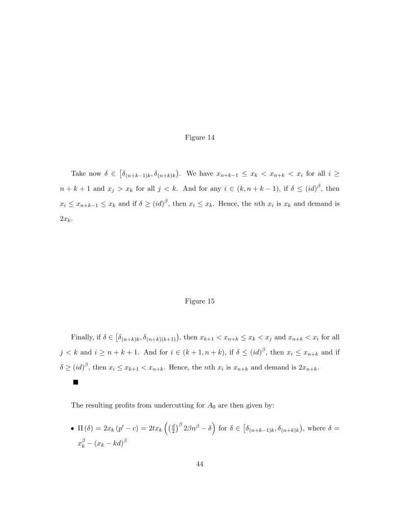
Figure 14

Take now δ ∈£δ(n+k−1)k, δ(n+k)k

¢. We have xn+k−1 ≤ xk < xn+k < xi for all i ≥

n + k + 1 and xj > xk for all j < k. And for any i ∈ (k, n+ k − 1), if δ ≤ (id)β, then

xi ≤ xn+k−1 ≤ xk and if δ ≥ (id)β, then xi ≤ xk. Hence, the nth xi is xk and demand is

2xk.

Figure 15

Finally, if δ ∈£δ(n+k)k, δ(n+k)(k+1)

¢, then xk+1 < xn+k ≤ xk < xj and xn+k < xi for all

j < k and i ≥ n + k + 1. And for i ∈ (k + 1, n+ k), if δ ≤ (id)β, then xi ≤ xn+k and if

δ ≥ (id)β, then xi ≤ xk+1 < xn+k. Hence, the nth xi is xn+k and demand is 2xn+k.

The resulting profits from undercutting for A0 are then given by:

• Π (δ) = 2xk (p0 − c) = 2txk

³¡d2

¢β2βnβ − δ

´for δ ∈

£δ(n+k−1)k, δ(n+k)k

¢, where δ =

xβk − (xk − kd)β

44

Figure 7.1: Figure 16

• Π (δ) = 2txn+k

³¡d2

¢β2βnβ − δ

´for δ ∈

£δ(n+k)k, δ(n+k)(k+1)

¢, where δ = xβn+k −

((n+ k) d− xn+k)β

We need to compare these profits from undercutting with the profit A0 obtains by

charging p∗ (n) like everyone else, i.e. with Π (p∗ (n)) = 21−βtβ (nd)β+1. The difference

with the case of linear transportation costs is that here the profit function is continuous in

δ, or alternatively in p0.

Consider the following deviation:

δ = δ(n+1)1 =

µd

2

¶β ³(n+ 2)β − nβ

´x1 = xn =

(n+ 2) d

2

The resulting profit is:

Π¡δ(n+1)1

¢= 2−βtdβ+1 (n+ 2)

³2βnβ − (n+ 2)β + nβ

´

45

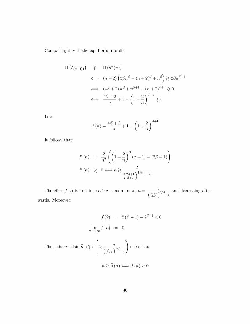
Comparing it with the equilibrium profit:

Π¡δ(n+1)1

¢≷ Π (p∗ (n))

⇐⇒ (n+ 2)³2βnβ − (n+ 2)β + nβ

´≷ 2βnβ+1

⇐⇒ (4β + 2)nβ + nβ+1 − (n+ 2)β+1 ≷ 0

⇐⇒ 4β + 2

n+ 1−

µ1 +

2

n

¶β+1

≷ 0

Let:

f (n) =4β + 2

n+ 1−

µ1 +

2

n

¶β+1

It follows that:

f 0 (n) =2

n2

õ1 +

2

n

¶β

(β + 1)− (2β + 1)!

f 0 (n) ≷ 0⇐⇒ n ≷ 2³2β+1β+1

´1/β− 1

Therefore f (.) is first increasing, maximum at n = 22β+1β+1

1/β−1and decreasing after-

wards. Moreover:

f (2) = 2 (β + 1)− 2β+1 < 0

limn−→∞

f (n) = 0

Thus, there exists−n (β) ∈

"2, 2

2β+1β+1

1/β−1

!such that:

n ≥ −n (β)⇐⇒ f (n) ≥ 0

46

We have thus proven that for n ≥ −n (β) the following undercutting strategy for A0 is

profitable:

p0 = p− tδ(n+1)1

Therefore, for all n ≥ −n (β) there is no symmetric price equilibrium.

8. REFERENCES

Deneckere, R. and Rothschild, M. (1992), "Monopolistic Competition and Preference Di-

versity", Review of Economic Studies, 59, 361-373.

Dixit, A. and Stiglitz, J. (1977), "Monopolistic Competition and Product Diversity",

American Economic Review, 67, 297-308.

Perloff, J. and Salop, S. (1985), "Equilibrium with Product Differentiation", Review of

Economics Studies, 52, 107-120.

Salop, S. (1979), "Monopolistic Competition with Outside Goods", Bell Journal of

Economics, 10, 141-156.

Sattinger, M. (1984), "The Value of an Additional Firm in Monopolistic Competition",

Review of Economic Studies, 51, 321-332.

47