monitoring surface water treatment processes · 2.0 surface water treatment rules surface water...
TRANSCRIPT

Monitoring Surface Water
Treatment Processes
December 2019
DOH Pub 331-620

Table of Contents
1.0 Monitoring Surface Water Treatment Processes ................................................................................................................. 1
2.0 Surface Water Treatment Rules .................................................................................................................................................. 1
3.0 Surface Water Treatment Rule Monitoring Plan .................................................................................................................. 2
4.0 Acceptable Analytical Methods .................................................................................................................................................. 2
5.0 Collecting Samples .......................................................................................................................................................................... 3
6.0 Measuring Water Quality and Physical Parameters ............................................................................................................ 4
6.1 About pH ........................................................................................................................................................................................ 4
6.1.1 Where, When, and How to Measure pH for CT Compliance ............................................................................ 5
6.1.2 Calibration and Verification of pH Meters ............................................................................................................... 5
6.2 Temperature .................................................................................................................................................................................. 6
6.3 Free and Total Chlorine Residual........................................................................................................................................... 7
6.3.1 Measuring Chlorine Residual for CT Compliance ................................................................................................. 7
6.3.2 Distribution Entry Point Residual ................................................................................................................................ 7
6.3.3 Distribution System Residual ........................................................................................................................................ 8
6.3.4 Measurement Technique and Quality Control for Chlorine Residual ........................................................... 8
6.4 Turbidity .......................................................................................................................................................................................... 9
6.4.1 Filtered System Turbidity Monitoring........................................................................................................................ 9
6.4.2 Turbidity Data Recording and SCADA for Rapid Rate Filtration ................................................................... 11
6.4.3 Unfiltered System Turbidity Monitoring ................................................................................................................. 12
6.4.4 Measurement Technique and Quality Control for Turbidity ........................................................................... 12
6.5 Elements of Contact Time: Flow, Volume, Baffling Efficiency .................................................................................. 13
6.5.1 Flow meters and Peak Hourly Flow .......................................................................................................................... 13
6.5.2 Verify Contact Volume and Basin Dimensions ..................................................................................................... 15
6.5.3 Verify and Inspect Tank Baffling ................................................................................................................................ 15
6.6 Calculate Daily Inactivation Ratio ....................................................................................................................................... 15
6.6.1 Special Situations for Calculating Inactivation Ratio ......................................................................................... 16
6.7 Other Water Quality Parameters: Alternative Disinfectants ..................................................................................... 17
6.7.1 Ozone .................................................................................................................................................................................. 17
6.7.2 Chlorine dioxide ............................................................................................................................................................... 18

6.7.3 Chloramines ...................................................................................................................................................................... 19
6.7.4 UV .......................................................................................................................................................................................... 19
6.8 Special Monitoring for Alternative Filtration Technologies ..................................................................................... 20
6.8.1 Membrane Filtration ...................................................................................................................................................... 20
6.8.2 Bag and Cartridge Filtration ........................................................................................................................................ 21
7.0 Critical Alarms and Alarm Set Points ...................................................................................................................................... 22
8.0 Standard Operating Procedures ............................................................................................................................................... 23
9.0 Recordkeeping and Reporting .................................................................................................................................................. 23
10.0 Conclusions .................................................................................................................................................................................... 24
Appendix .................................................................................................................................................................................................. 25
A.1 Sample SWTR Monitoring Plan (Small Slow Sand Filter Plant) .................................................................................... 26
A.2 Sample SWTR Monitoring Plan (Rapid Rate Conventional Plant) ............................................................................... 27
A.3 Acceptable Methods for Measuring pH, Temperature, and Turbidity ...................................................................... 28
A.4 Acceptable Methods for Measuring Residual Disinfectant ........................................................................................... 29
A.5 Sample SOP: Measuring Turbidity—Hach 2100Q Portable Turbidimeter (0–1000 NTU) .................................. 30
A.6 Sample SOP: Measuring Free Chlorine Residual—Hach Pocket Colorimeter II (0.02-8 mg/L) ........................ 32
A.7 Sample SOP: Check of Chlorine Test Kit Using Standard Additions-Pocket Colorimeter II .............................. 33
Example Standard Additions Data Table ................................................................................................................................ 34
A.8 Sample SOP: Measuring pH Using Hach SensION+ Portable Test Kit and 5050T Probe .................................. 35
A.9 Recommended On-line Turbidimeter Settings and Monitoring Guidelines: Rapid Rate and Membrane
Filtration .................................................................................................................................................................................................... 36
A.10 Recommended On-Line Turbidimeter Settings Unfiltered Sources and Slow Sand, DE and Bag Filtration
Plants ......................................................................................................................................................................................................... 37
A.11 Plumbing Sample to a Process Analyzer—Thoughts to Ponder ............................................................................... 38
A.12 Typical Alarm Set Points ........................................................................................................................................................... 41
References................................................................................................................................................................................................ 43
If you need this publication in an alternative format, call 800.525.0127 (TDD/TTY call
711). This and other publications are available at doh.wa.gov/drinkingwater.

1
1.0 Monitoring Surface Water Treatment Processes
Operators monitor surface water treatment processes to confirm they operate
effectively and produce safe water. For the results to be meaningful, every
operator must be able to accurately measure key water quality and physical
parameters including pH, temperature, chlorine residual, turbidity, and the
parameters that effect contact time: flowrate, contact chamber volume, and
baffling efficiency. While this document focuses on surface water treatment
facilities, most of the information applies equally to any water quality monitoring
performed for all public water systems, regardless of source type.
Many states report issues with the water quality data their water systems collect
and report. In two separate studies completed in Washington, we found issues
with data measurement, recording, or reporting at every participating treatment
plant. Nationwide, 15 data integrity workshops held over the past six years found
issues at even well operated plants. These findings led us to increase our focus on
data integrity, with the goal that all water quality information gathered is
trustworthy over its entire life cycle—from the point of sample collection through
analysis, storage, retrieval, and reporting to managers, customers, and regulatory
agencies.
Achieving quality data you can trust depends on proper installation and
maintenance of your equipment, robust calibration and verification procedures,
accurate reporting, and integration with SCADA systems. Written standard
operating procedures (SOPs) ensures everyone in your utility has access to
industry best practices and establishes your expectation that everyone will do
things the right way every time.
For each parameter used to monitor surface water treatment plant performance,
pay close attention to changes that occur over time, unexpected changes, or
changes that can’t be explained. Ask yourself; “how do I know this measurement
or reading is accurate?” Use the calibration and verification procedures described
in Section 6.0 to answer that question.
2.0 Surface Water Treatment Rules
Surface water sources and sources designated as groundwater under the direct
influence of surface water (GWI) carry a high microbial risk. As a result, the basic
treatment framework requires the following minimum level of treatment.
2-log removal or inactivation of Cryptosporidium oocysts.
3-log removal or inactivation of Giardia lamblia cysts.
4-log removal or inactivation of viruses.
For poorer quality surface water sources with the highest risk of contamination,
and for water systems operating under a limited alternative to filtration, state
rules may require a greater level of treatment than these basic requirements.
Data integrity means that
the water quality
information gathered is
trustworthy over its entire
life cycle—from the point
of sample collection,
through analysis, storage,
retrieval, and reporting to
managers, customers,
and regulatory agencies.

2
Regulatory requirements for surface water treatment facilities (Chapter 246-290
WAC Part 6) stem from multiple federal rules developed over the past three
decades.
Surface Water Treatment Rule (SWTR).
Interim Enhanced Surface Water Treatment Rule (IESWTR).
Long Term 1 Enhanced Surface Water Treatment Rule (LT1ESWTR).
Filter Backwash Recycle Rule (FBRR).
Long Term 2 Enhanced Surface Water Treatment Rule (LT2ESWTR).
Effective implementation of these rules and protection of consumers depends on
a multiple barrier framework: source water protection, filtration, disinfection, and
safeguarding treated water within the distribution system—with well-trained,
certified operators overseeing all.
3.0 Surface Water Treatment Rule Monitoring Plan
A written monitoring plan ensures you measure the right parameters at the
correct frequency and location. You stay on track with regulatory requirements
and ensure a smooth transition when staff changes occur.
Your SWTR monitoring plan should reflect the type of treatment installed and
population size served. WAC 246-290-664 outlines monitoring requirements for
surface water treatment facilities with filtered sources, and WAC 246-290-694 for
unfiltered sources. If you use an alternative filtration technology such as
membranes or bag filters, or an alternative disinfectant like UV or ozone, you will
have additional monitoring requirements established during your plant’s design
approval process. Contact your Department of Health Office of Drinking Water
(ODW) regional office if you have questions about your system’s requirements.
Eastern Regional Office 509-329-2100
Northwest Regional Office 253-395-6750
Southwest Regional Office 360-236-3030
Besides the minimum monitoring requirements in the SWTR, your plant operators
conduct other water quality monitoring for process control. These are specific to
your facility and this guidance does not cover them.
If you have an undocumented or out-of-date monitoring plan, take time now to
correct this. Then post it at your treatment plant and review it with your regional
engineer during the next sanitary survey. To help you get started, see the two
sample monitoring plans in Appendix A.1 and A.2.
4.0 Acceptable Analytical Methods
For consistent and accurate measurements, you must follow EPA-approved or
standard methods. Appendix A.3 and A.4 list the methods approved for SWTR
compliance in Washington. These tables include examples of commercially

3
available test kits or lab equipment. This is not a comprehensive list. If you have a
question about a piece of equipment that does not appear here, contact the
manufacturer and ask whether it meets one of the approved methods.
DOH does not allow the use of test strips or visual color-comparator-style test kits
for pH and chlorine, because they do not provide accurate and consistent results.
5.0 Collecting Samples
A typical sample is only a tiny fraction of the water delivered to customers. Sample
location, hold time, and sampling technique all determine whether analysis results
will accurately represent the water treated or delivered to customers.
The first step in collecting a representative sample is choosing the correct
location, which accurately reflects what you are measuring. The sample must be
well-mixed, but avoid locations with turbulent flow conditions that may entrain
air—such as near pumps, valves, and pipe fittings. If there is a chemical injection
point upstream, place the sample point downstream after all the chemical mixes.
Consider moving the sample point upstream if the added chemical might
interfere with the measurement.
When installing sampling taps, it is best to tap the side of the pipe (+/- 45
degrees). This avoids any trapped air at the top of the pipe and sediment that
may settle on the bottom. Use a sampling quill to sample near the center of the
pipe and avoid more stagnant conditions and biofilm fouling on the inside
surface.
Timing is critical for many water quality parameters. Measure temperature and
pH immediately. Perform chlorine residual measurements as soon as possible.
You can hold turbidity samples for several minutes, but swirl the sample if
particles are present and settling out.
Don’t aerate the sample because that will change the sample result. Remove
aerators and control the sample flow to produce a smooth pencil-sized
stream. When collecting samples, rinse the sample container or vial and cap
three times with sample water before filling to the appropriate measurement
level.
When installing online analyzers, avoid pumping the sample if you can,
because pumps can entrain air or change the characteristics of the sample. If
you must pump the sample, avoid pumps that cause pulsation such as piston,
diaphragm, or peristaltic pumps, or use a pulsation dampener. Take steps to
minimize sample delay. Aim for a sample delay of one minute or less. Keep
sample lines as short as possible and use the smallest diameter sample line
that will deliver the required flow to the instrument. This will decrease sample
delay and discourage biofilm. Replace sample tubing regularly, especially if
you have high levels of iron or manganese.
Follow the manufacturer’s instructions when installing online monitoring
equipment. It is important to control flow and pressure for all instruments, but
Plumbing Process Analyzers
Choose a representative
location.
Tap the side of the pipe (+/-
45) and use a sampling
quill.
Don’t mix and match
plumbing materials.
Keep sample lines short (less
than 1 minute sample delay
is ideal).
Replace tubing regularly.
Avoid pumping if you can.
Control flow and pressure.

4
especially for turbidimeters, particle counters, and amperometric chlorine
analyzers. See Appendix A.11 for more information.
6.0 Measuring Water Quality and Physical Parameters
Most surface water treatment plants use a combination of filtration and
disinfection. To ensure these treatment processes operate effectively, all surface
water treatment plants measure turbidity and distribution system chlorine
residual. Systems using free chlorine for primary disinfection, measure pH and
temperature in addition to free chlorine residual because the effectiveness of
chlorine depends on these parameters. Systems using alternative disinfectants
such as ozone, chlorine dioxide, or ultraviolet radiation (UV) have special
monitoring requirements unique to those technologies.
Failure to use proper methods and procedures can cause significant errors. A
study of treatment plants in Washington found that pH, temperature, and
chlorine residual measurement errors caused calculated Giardia inactivation
ratios to be off by up to 40 percent.
6.1 About pH
pH is a measurement of the hydrogen ion concentration. It represents the relative
acidity of an aqueous solution and is a negative logarithmic function. This means
that every one-unit decrease in pH represents a ten-fold increase in acidity. For
example, a pH 6 solution is ten times more acidic than a pH 7 solution. The most
important thing to remember is that free chlorine disinfecting power depends on
pH—the lower the pH, the more effective the chlorine.
When you add chlorine to water, it forms hypochlorous
acid (HOCl) and hypochlorite ion (OCl-), the two
components of free chlorine. HOCl is the much stronger
disinfectant—more than three times more powerful than
OCl-—in inactivating Giardia cysts. As seen in Figure 1, the
relative amount of these two compounds depends on pH.
At pH 6, for example, more than 95 percent of free
chlorine is present as HOCl. At pH 9, less than 5 percent of
free chlorine is HOCl. For these reasons, you need
accurate pH measurement to ensure disinfection is
effective.
In addition to its role in disinfection, pH monitoring is
important because it indicates whether you are
maintaining optimal conditions for other installed
treatment. For example:
Some coagulants work best in certain pH ranges.
Removal of inorganics and organics depends on pH.
Minimum pH requirements may be part of optimal corrosion control
treatment under the Lead and Copper Rule.
Figure 1
0%
10%
20%
30%
40%
50%
60%
70%
80%
90%
100%0%
10%
20%
30%
40%
50%
60%
70%
80%
90%
100%
5 6 7 8 9 10
% O
Cl-
% H
OC
l
pH
at 20C

5
When adding pH adjustment chemicals, pH-monitoring controls chemical
feed pumps and helps maintain dosages in the correct ranges.
Along with your alarm system, pH monitoring helps detect chemical
overfeeds.
6.1.1 Where, When, and How to Measure pH for CT Compliance
Surface water systems using free chlorine for primary disinfection must measure
pH at the end of each disinfection sequence. If you adjust pH part way through a
chlorine contact basin, you’ll need multiple monitoring points for representative
sample results. Measure pH at least once per day during peak hourly flow. If you
take multiple samples during the day or monitor continuously, and flow through
the contact basin is relatively constant, you may use the highest pH value for the
day in your CT calculation.
pH measurements are sensitive to both time and temperature. If you collect a
sample and don’t analyze it right away, pH will change as the sample is
exposed to air. Likewise, pH measurements are not stable and reproducible
when the sample temperature changes. For these reasons, measure your field
samples in the field. Do not transport them back to the lab for analysis.
Before taking a grab sample measurement, allow the pH probe to come to the
same temperature as the water you’re sampling. Do this by letting the probe
sit in a large container of the sample water for at least five minutes. Then
collect a fresh water sample and take a reading.
The sidebars list tips for accurate grab and online pH measurements.
6.1.2 Calibration and Verification of pH Meters
You must calibrate your portable or laboratory pH meter regularly. If your unit
does not include a calibration feature, replace it with one that does. Follow the
calibration instructions in your instrument manual. When calibrating, use at
least two buffers, ideally bracketing the pH of your water—one higher, one
lower. Pay strict attention to expiration dates and store buffers in closed
containers. Avoid storing them close to a window or heat source. Be aware
that pH 10 buffers are unstable and have a limited shelf life, so if you choose
to use pH 10, make sure you have robust quality control procedures.
Refrigerate pH 10 buffer and allow it to come to room temperature prior to use.
For typical pH ranges found in drinking water, a pH 8 buffer may be a better
choice.
Verify your meter between calibrations with a single-point verification using fresh
buffer in the range of measurement. Don’t use the same buffer you used to
calibrate the instrument. For example, if you normally calibrate with pH 4 and 7
buffers, you could choose a pH 6.86 buffer by a different manufacturer for your
Measuring pH
Grab Samples
Calibrate your meter with at
least two buffers every day
you use it.
Use fresh (unexpired)
calibration solutions.
Allow the probe to adjust to
the water temperature
Measure your sample
immediately after collecting
it. Avoid transporting the
sample to another location.
Gently swirl or stir the
sample gently to minimize
air bubbles.
When measuring low-
conductivity water (<100
umhos), consider using a
specialized probe.

6
verification check. Recalibrate if the pH meter does not accurately read the
buffer (within +/-0.1 pH units).
EPA-approved methods vary somewhat on the minimum frequency of
calibration for portable or bench-top pH meters. Most water quality labs
follow standard methods (4500H+) and calibrate their pH meters each day
they are used. EPA Method 150.3 allows weekly calibration, as long as a daily
verification check shows the probe has not drifted. Although this practice is
allowable, we recommend following best industry practice by calibrating
daily.
Some utilities use online pH meters for compliance monitoring. According to
EPA Method 150.3, you must calibrate online pH analyzers at least once per week,
whenever you do any maintenance on the probe, or whenever you no longer
obtain a good verification. Like laboratory or portable equipment, calibrate online
meters with at least two buffers that bracket the expected pH of the water.
You must verify online pH meters every day (EPA Method 150.3). Do this by grab
sample comparison with a portable or laboratory instrument or by removing the
probe and measuring a sample of known concentration, such as a
commercial pH buffer in the range of measurement. You must recalibrate the
probe if the two instruments are more than 0.2 units apart or readings vary
by more than +/-0.1 units from the known standard.
When comparing a continuous online instrument to a bench top unit, it is
critical to minimize or eliminate differences between the two water samples.
Temperature, flow characteristics across the probe, and trapped air can affect
resulting pH values. Carrying samples from the online analyzer to the lab
introduces errors. Instead, bring your portable pH meter to the online
analyzer. Allow the portable pH probe to come to the same temperature as
the water before taking a reading. One excellent approach is to install an
empty flow-through cell next to the pH analyzer, as shown in the photo
(right) from the Cedar River Water Treatment Plant. This allows you to place
the portable probe into the sample flow where it can adjust to the water
temperature and measure the exact same water as the online probe without
disturbing it. If you do not have this type of sample setup, we recommend
installing one.
6.2 Temperature
Chlorine disinfection is less effective at lower temperatures. For example, it takes
more than three times more chlorine residual to inactivate the same amount of
Giardia cysts at 5º C than at 20º C (pH 7). For most surface water systems in
Washington, winter cold-water temperatures (2-5 ºC) produce the most
challenging conditions for meeting SWTR disinfection requirements.
You must measure temperature for CT compliance at the end of each disinfection
sequence and at least once per day during peak hourly flow. If you take multiple
samples during the day or monitor continuously, and flows entering and leaving
the contact basin are nearly the same, it is acceptable to use the lowest daily
temperature value in your CT calculation.
Measuring pH: Online
Analyzers
Make sure your instrument has
temperature compensation.
Provide stable flow and
pressure
Calibrate the probe at least
every week.
Verify the probe every day.

7
Temperature changes rapidly after you collect a sample, so don’t delay in reading
the thermometer. You can also use a properly calibrated online temperature
probe.
Once or twice per year, check the thermometer against an NIST-certified
precision thermometer. NIST is the U.S. National Measurement Institute. NIST
certification means a certified laboratory calibrated the device using an NIST
reference standard and it meets exacting requirements.
Do a quick thermometer verification check by placing it in a beaker of ice water. It
should read 0º C. Verify an online probe by comparing it to another properly
calibrated thermometer.
6.3 Free and Total Chlorine Residual
Water systems use chlorine to kill pathogens such as Giardia and viruses
(primary disinfection), and to maintain a protective residual and prevent
biological regrowth in the distribution system (secondary disinfection).
Operators of chlorinated systems must measure free or total chlorine
residual at three locations: 1) the end of each disinfectant sequence; 2) the
distribution entry point; and 3) representative points in the distribution
system.
6.3.1 Measuring Chlorine Residual for CT Compliance
You must take chlorine residual measurements for CT compliance (Giardia
and virus inactivation) from the end of each disinfection sequence, at least
once per day during peak hourly flow. If using grab samples, use the
previous day’s records to estimate when peak hourly flow will occur. If
monitoring continuously, use the value during peak hourly flow to calculate
the daily inactivation ratio. If flows entering and leaving the contact basin
are nearly the same, you may use the lowest daily value in your CT
calculation.
6.3.2 Distribution Entry Point Residual
Most systems with a single disinfection sequence use the CT compliance
point for distribution entry. Larger systems (population above 3,300) must
continuously measure free chlorine residual at the distribution entry point
and report the lowest daily value. If continuous monitoring is required and
the analyzer fails, you must take grab samples every four hours and have
the analyzer repaired and running within five working days.
Smaller systems may use grab sampling at the distribution entry point, one to
four times per day, depending on population served. Systems using grab
sampling take one sample at peak hourly flow and space the remaining samples
Chlorine Residual Tips
Grab Sampling
Measure free chlorine residual,
unless you use chloramines.
Clean sample vials thoroughly
after every use. Using lab
wipes or lint free wipes can
help keep your sample vials
scratch free.
Periodically replace sample
vials (when scratched or
discolored).
Discard expired reagents.
First, read the blank, then the
sample. Use the same vial to
zero the instrument and
measure the sample.
For free chlorine, read the
result promptly (within one
minute of adding the reagent).
Pay attention to low and high
range settings on your
instrument.
Follow the instructions that
came with your instrument!

8
over the period that the plant produces water. Record the lowest grab
sample result.
For all systems: If the free chlorine residual at the distribution entry point
ever drops below 0.2 mg/L, you must call your DOH regional office as soon
as possible, but no more than 24 hours after you learn of the event.
6.3.3 Distribution System Residual
All systems must measure distribution chlorine residual at representative
locations throughout the distribution system. Do this at least daily and at
the same time and location as you collect each coliform sample. Most
systems measure free chlorine. However, systems using chloramines for a
secondary (distribution) residual must measure total chlorine or combined
chlorine (total minus free) in the distribution system.
6.3.4 Measurement Technique and Quality Control for Chlorine Residual
Tips for accurate grab and online chlorine measurements are in the sidebars. There
is a detailed discussion of plumbing for process analyzers in Appendix A.11.
If you use a portable DPD test kit to measure grab samples, verify the instrument
at least once every quarter. Do this by comparing it to a laboratory instrument, or
by measuring a sample with a known concentration, a chlorine standard, or other
method the manufacturer recommends. If the unit does not read accurately (+/-
0.1 mg/L), you must repair or replace it. Use a secondary standard to verify your
instrument is working, but remember that a secondary standard only checks the
instrument. It does not check your reagents, your glassware, or your technique.
Immediately after opening a fresh batch of DPD reagent, run a reagent blank. First,
zero the instrument with a sample cell filled with deionized or distilled water, then
add reagent to the sample and take a reading. Write the resulting value on the
DPD container. Subtract this value from all future sample results using this batch
of reagent. If the reagent blank reads high, more than 0.01 or 0.02 mg/L, there
may be a quality control problem with the reagent and you should replace it. The
photo below shows three containers of powdered DPD reagent with the same lot
number. Along with the obvious difference in color, the reagent blanks made from
these samples ranged from 0.05 mg/L on the left to 0.13 mg/L, on the right.
Chlorine Analyzer Tips
Install the equipment properly
(refer to the equipment
manual).
Follow the manufacturer’s
recommended maintenance
schedule.
Verify your instrument at least
every five days (should be
within 15 percent or 0.1 mg/L,
whichever is greater)
Check the sample flowrate
(Cl-17)
Photo courtesy of Emilia Blake, Skagit County PUD.

9
If you use an online chlorine analyzer, you must verify it against a laboratory or
portable instrument at least once every five days. Results must be within +/- 0.1
mg/L or 15 percent, whichever is larger. Water systems in Washington usually use
colorimetric or amperometric chlorine analyzers. Colorimetric online analyzers,
such as the Hach Cl-17, rely on factory calibration, proper installation, and regular
maintenance to produce accurate results. Amperometric analyzers require less
maintenance, but rely primarily on verification checks to ensure accuracy. When
using an amperometric probe or sensor for SWTR compliance, you must follow
the detailed quality control procedures described in EPA method 334.0. These
include proof of performance and routine quality control procedures for the grab
sample reference method, each sample collector, and each online analyzer. If you
use amperometric probes, read the complete method for details.
Amperometric free chlorine sensors generally measure only HOCl, not OCl-. In
normal pH ranges of most water systems (7.0 to 8.0), the ratio of the two species
of free chlorine is very sensitive to pH (see Figure 1). For this reason,
amperometric analyzers used in drinking water should always have continuous
pH compensation.
At pH 8.0 or greater, HOCl is only a small part of free chlorine (< 20 percent). In
this setting, small changes in pH or chlorine residual can affect amperometric
sensor accuracy and cause it to drift, even with pH compensation. Because the
DPD method measures all free chlorine species and is independent of pH, it may
be a better choice in this case.
6.4 Turbidity
Turbidity is a measurement of scattered light from suspended solids. The higher
the intensity of scattered light, the higher the turbidity. For rapid rate filtration,
turbidity measurements show how effectively your filtration system removes
particles, including pathogens like Giardia and Cryptosporidium. At slow sand,
diatomaceous earth (DE), and bag filtration plants, operators use turbidity
measurements to verify filtration processes are working correctly and removing
pathogenic organisms from the source water. In both unfiltered and filtered
sources, turbidity monitoring also verifies that turbidity does not reach levels that
could interfere with disinfection.
Most surface water systems use continuous meters for turbidity monitoring. A
surprising number of factors affect the accuracy of the turbidimeter data
generated, recorded, and reported, such as instrument settings, physical
locations, electronic data manipulation, operational practices, and human actions.
See Appendix A.9 and A.10 for recommended settings for online turbidimeters.
6.4.1 Filtered System Turbidity Monitoring
Systems with filtered surface water sources measure turbidity at up to four
locations: the untreated source water, after the settling or clarification process,
after each individual filter, and in the combined filter effluent (CFE).
Collect source turbidity samples before disinfection and chemical addition. If
using grab samples, collect a representative sample after plant startup when it’s

10
running smoothly. If monitoring continuously, record the daily average value on
the monthly operations report (MOR). If your system recycles backwash water to
the head of the plant, measure raw turbidity prior to (upstream from) the recycle
point. You also should measure recycled water turbidity for process control
purposes.
If your plant has a settling or clarification process, we recommend measuring
effluent turbidity from each settling or clarification basin. This can identify
problems such as short circuiting, which may cause one basin to perform more
poorly than another. If monitoring continuously, record the daily average value
on your MOR. If using grab samples, collect a representative sample after startup
when the plant is running smoothly. If you collect multiple grab samples, report
the average value.
The CFE is a point that best represents the water quality produced by all filters
combined. Because of differences in filter piping and clearwell configuration, the
exact CFE location may vary from plant to plant. In general, the best place is a
common header pipe that collects water from individual filters before they flow
into the clearwell. Because of piping differences and layouts at each plant,
operators sometimes struggle to find a suitable CFE location. We encourage
systems with only two filters and no good CFE sampling location to report the
highest individual filter effluent (IFE) reading as the CFE on their MOR. Many of
these systems operate only one filter during low demand periods, so there is no
difference between IFE and CFE during these periods.
Larger systems with multiple filters, all discharging directly and separately into a
common clearwell, should use a pumped sample from an appropriate clearwell
location. The sample location should have completely mixed water from all filters
and be as close as possible to the point where the filters discharge into the
clearwell. Appendix A.11 discusses sample pump selection.
Filtered systems must report turbidity readings to DOH each month (WAC 246-
290-666). Although the rules allow daily grab sampling for small systems using
simple filtration technologies, such as slow sand or bag filtration, most systems
monitor turbidity continuously using online analyzers.
For rapid-rate filtration plants, you must record the CFE turbidity readings every
four hours and report them on your MOR. For plants operating continuously,
report the value at midnight, 4 a.m., 8 a.m., and so on. For other plants, report the
first value within 15 minutes after initial plant startup (filtered water flowing to
the clearwell or distribution) and then at exactly four-hour intervals for as long as
the plant continues to run. If your plant does not operate continuously
throughout the day, record a new initial turbidity reading within 15 minutes of
plant restart, and then every four hours thereafter. The daily maximum CFE
turbidity measurement is the highest turbidity of water your plant produces and
sends to consumers at any time during the calendar day. It is not the maximum
of the four-hour readings.
Rapid rate filter plants using direct, inline, or conventional filtration also must
measure turbidity continuously from each individual filter. For process
optimization, locate IFE sample points immediately after the filters and before

11
filter to waste piping to allow turbidity monitoring during filter to waste. Record
IFE turbidity results at least every 15 minutes. If IFE turbidity values exceed
0.5 NTU in two consecutive measurements, you must report this on the MOR. Do
not report IFE turbidity measurements taken during backwash or filter to waste.
6.4.2 Turbidity Data Recording and SCADA for Rapid Rate Filtration
Most systems record turbidity data on a SCADA computer in a data log. SCADA
system data logs must be able to handle long-term turbidity data storage needs
based on monitoring requirements described in the previous section. For
example, rapid rate plants must store and be able to easily extract 15-minute IFE,
four-hour CFE and daily maximum CFE results. Data storage systems also must
meet minimum turbidity data-retention requirements of at least five years.
The Washington Treatment Optimization Program (TOP) is an effort to improve
performance of rapid-rate surface water treatment facilities. TOP focuses on
particle removal and disinfection to maximize public health protection from
microbial contaminants. ODW adopted performance goals for all rapid-rate
surface water treatment plants in the state. For turbidity data, these include:
Filtered water is less than 0.10 NTU 95 percent of the time, based on
maximum daily values recorded.
Filtered water is below 0.10 NTU within 15 minutes of putting filter in to
production.
Settled water turbidity is less than or equal to 2 NTU 95 percent of the
time when annual average source turbidity exceeds 10 NTU.
Settled water turbidity is less than or equal to 1 NTU 95 percent of the
time when annual average source turbidity is less than or equal to
10 NTU.
The system monitors raw water turbidity at least every four hours, and
continuously records effluent turbidity for each filter and the combined
filter effluent.
To help plant operators achieve turbidity optimization goals, you should log data
more frequently than required. For optimization, capture and record data at
intervals of one minute or less, or record maximum IFE and CFE values for each
15-minute period. You should create the data log daily in an easily accessible
format (e.g., csv, xlsx), including date, time, and turbidity value for each
continuous-reading turbidimeter.
Tag logged turbidity data to identify plant operating-conditions (filter-to-
clearwell, filter-to-waste, backwash, out of service, and so on). Keep data log files
in an easily accessible directory. Program SCADA monitoring systems to allow
operators to create their own trend lines using flexible turbidity and time scales.
The SCADA system also should allow operators flexibility to create plant-specific
control screens showing selected trend lines (selected filter IFE turbidity, filter
flow rate, and valve open-closed positions for the selected filter in the same
view).

12
6.4.3 Unfiltered System Turbidity Monitoring
Systems with unfiltered surface water sources must continuously measure
turbidity immediately before the first point of primary disinfectant application
(WAC 246-290-694). The 5 NTU maximum turbidity limit for unfiltered systems is
designed to prevent particles from shielding microorganisms from disinfection.
This is extremely important, because these systems lack a filtration barrier. Report
the maximum turbidity value for the day on the MOR.
In unfiltered surface water systems, source water turbidity values above 1.0 NTU
trigger additional coliform monitoring requirements. See WAC 246-290-694(1)
and (3).
6.4.4 Measurement Technique and Quality Control for Turbidity
When using portable or laboratory turbidimeters, better technique usually
leads to lower and more accurate measurements. Tips for accurate grab-
sample turbidity measurements are in the sidebar. Section 5.0 and Appendix
A.11 have general tips on plumbing process analyzers.
Turbidimeter calibration and verification requirements are in WAC 246-290-
638(4). You must:
Calibrate all turbidimeters using a primary standard according to the
manufacturer’s instructions.
Calibrate devices that use an incandescent light source at least once
per quarter.
Calibrate devices that use an LED or laser light source at least
annually (or more frequently per the manufacturer’s
recommendation).
In addition to primary calibration, you must verify continuous online
turbidimeters at least weekly by comparing them to a calibrated bench-top
turbidimeter. This verifies that continuous units maintain accuracy between
quarterly calibrations, and maintains operator proficiency with the bench-
top unit. If a continuous unit fails, you must use the bench-top unit for
ongoing turbidity monitoring.
Results between the continuous and bench-top units may not match
exactly. Generally, bench-top units read a higher turbidity. An acceptable
difference between the values is the larger of +/- 0.05 NTU or 10 percent. Record
weekly verification values in a turbidimeter-specific maintenance logbook. You
may use secondary standards, such as the Hach ICE-PIC® or similar device, in lieu
of a grab sample verification.
If your turbidimeter uses an incandescent light source, you will need to replace
the lamp periodically (usually annually). Check your equipment manual for this
and other required maintenance.
Turbidity Tips—Grab Sampling
Calibrate your instrument
using a primary standard.
Replace calibration standards
when expired.
Use clean scratch-free sample
cuvettes. Replace them often.
Use laboratory wipes only (not
your shirt) to wipe the cuvette
before placing it in the
instrument.
Use silicon oil to mask minor
imperfections, but be sure to
wipe off excess oil thoroughly
with a clean lab wipe.
Carefully follow instrument
manufacturer’s instructions.
Check the internet—many
manufacturers post useful
videos covering the proper
use and calibration of their
equipment.

13
6.5 Elements of Contact Time: Flow, Volume, Baffling Efficiency
Effectiveness of free chlorine disinfection depends directly on the length of time
chlorine is in water. This is known as contact time, or “T.” The SWTR establishes
disinfection levels that achieve the required inactivation of Giardia and viruses
under different water quality conditions. In SWTR “CT tables,” C is the residual
disinfectant concentration in mg/L, and T is the contact time in minutes. Section
6.6 describes how to use your actual available CT value, CTcalc and compare this
with the required CT value, CTrequired to calculate the inactivation ratio. You must
make this calculation each day your system produces water for the public.
Contact time (T) is not measured directly. It is calculated from flow, volume, and
the baffling efficiency of the contact basin, as follows.
Time = (Volume x Baffling efficiency)/Flowrate
Baffling efficiency is a measure of short-circuiting in the contact basin. The value
ranges from 0 to 1.0 and is established for each contact basin using a tracer study
or empirical calculation that ODW must review and approve. A higher baffling
efficiency means there is little or no short-circuiting in the basin. A low baffling
efficiency (0.1 or less) means significant short-circuiting, which reduces the
residence time in the basin.
A “bump test” is a quick way to determine whether your assumed contact time is
realistic. Temporarily increase the chlorine dose by 50 to 100 percent and see
how long it takes for the higher chlorine residual to reach the end of your contact
basin. If it is a lot different from the contact time used for that flow rate,
investigate further. You might have to change your high chlorine alarm set point
temporarily during the test. Remember to turn the chlorine feed pump back
down and restore the alarm set point when you’re done.
6.5.1 Flow meters and Peak Hourly Flow
Peak hourly flow is the greatest volume of water passing through the
disinfection contact chamber during any one hour in a consecutive 24-hour
period. It is not the absolute peak flow occurring at any instant during the
day. For a contact basin where water levels fluctuate, peak hourly flow is the
larger of the flow into the contact basin (from the treatment plant) and the
outlet flow (to the distribution system). Start by ensuring you have meters
installed to measure both the flow rate from the plant into the clearwell and
from the clearwell out to the distribution system.
Inaccurate flow measurements and false assumptions can be the largest source of
error in determining disinfection contact time. The best way to determine peak
hourly flow is by direct measurement using a properly installed and calibrated
water meter. The accuracy of meters can deteriorate with age; damaged or older
meters can produce incorrect readings. For accurate data, make sure your system
uses the correct type of meter, properly installed, and regularly inspected and
calibrated. For large source meters, Flowmeters in Water Supply (AWWA M33) is
a manual of practice accepted across the water industry. For smaller meters in use
at some very small facilities, refer to Water Meter Selection, Installation, Testing
When selecting, installing,
operating, calibrating, and
maintaining meters, you must
follow accepted industry
standards and manufacturer
information (WAC 246-290-
496 (3)).

14
and Maintenance (AWWA M6). For meter-specific information, consult the
equipment manufacturer’s relevant manual.
When selecting meters, consider the range of flow under which the system
operates, the size of the pipe, how much pressure loss you can tolerate, and your
automation and data recording needs. Your meter vendor should be able to help
you verify that you have the correct meter type for your application. Tables like
the one below can help you get started.
To get accurate results, you must install meters properly. One of the most
common meter installation mistakes is not allowing enough straight run pipe
upstream and downstream from the meter. Read the equipment manual carefully
and consult the manufacturer to make sure the installer followed correct
procedures.
Inspect and calibrate all meters periodically as part of a scheduled maintenance
program. Meters with moving parts require calibration more frequently. AWWA
M33 recommends that you recalibrate turbine or propeller meters every year.
Ultrasonic meters may need recalibration to account for pipe corrosion or scale
build-up that occurs over time. Consult your equipment manufacturer for specific
recommendations. Beware that flow meter calibration can change the
measurement range. If the 4 to 20 mA scaling is not adjusted to compensate
SCADA will display incorrect readings. After calibration, check the local meter
display against the SCADA screen and make sure the flowrates match.
Most Common Flow Meter Types General Guide
Flowmeter Type Pipe Sizes Pressure loss
Typical
accuracy in
percent
Required length
of straight pipe
upstream of
meter
Required length of
straight pipe downstream
of meter
Electromagnetic full
pipe meter
4”, 6”, 8”, larger
sizes available by
order
None ±0.5 % of rate
5 or less
Consult dealer and
specification sheet
2 or less
Consult dealer and
specification sheet
Electromagnetic
insertion meter 3” to 48” None
±1 % of full
scale
10 times pipe
diameter 5 times pipe diameter
Ultrasonic (time-of-
travel) 1” to 60” or more None
±2 % of full
scale
10 times pipe inside
diameter 5 times pipe inside diameter
Propeller 2” to 96” Low ±2 % of
reading 5 to 10 diameters 1 to 2 diameters
Positive displacement 5/8” to 2” High ±1.5 to 2 % Minimal Minimal
Vortex 2” to 20” Low to medium ±1 % of full
scale
10 times pipe
diameter 5 times pipe diameter
Adapted from Washington Department of Ecology, fortress.wa.gov/ecy/wrdocs/WaterRights/wrwebpdf/gsfps.pdf.
Some meters have internal diagnostics that can indicate a problem (Incontri,
2017). Consult with your equipment manufacturer to learn about your meter’s
capabilities. As a simple check, run a tank drawdown test once a year to confirm
your flow meter reads accurately.

15
6.5.2 Verify Contact Volume and Basin Dimensions
A surprising number of systems use incorrect volumes to calculate disinfectant
contact time. You must know the underlying assumptions contained in your
contact time calculation and independently verify the values are correct. If you
haven’t done so already, measure the disinfection contact tank or pipeline
dimensions and make sure the volume used to calculate contact time for your
system is correct.
If the water level in your contact basin fluctuates, you must know the tank
level to calculate volume accurately. If you base your calculation on a
minimum tank level, you must know what it is, and verify your tank does
not drop below it. Record the minimum tank level on your MOR every day
and verify it does not fall below that minimum level.
Operators use various devices to measure the depth of water in a
disinfectant contact tank. If you rely on an instrument, such as a pressure
transducer or ultrasonic level indicator for determining depth, check the
device at least once per year. Do so by directly measuring the water level
with a tape measure and comparing it to the instrument reading and the value
displayed on your SCADA screen, if you have one.
6.5.3 Verify and Inspect Tank Baffling
Some plants have flexible baffle curtains to create a maze-like pathway, reducing
short-circuiting and increasing disinfectant contact tank residence time. Inspect
these critical system components regularly. If visual inspection is possible without
entering the tank, check baffle curtains monthly. If visual inspection is difficult,
the simple bump test described above can confirm that the baffles are intact. At a
minimum, include baffle integrity as part of your comprehensive tank inspection
program. AWWA Standard G-200 recommends that storage tanks receive a
comprehensive inspection every three to five years.
6.6 Calculate Daily Inactivation Ratio
State and federal drinking water rules require that filtration and disinfection
systems together achieve at least 2-log (99 percent) removal or inactivation of
Cryptosporidium, 3-log (99.9 percent) removal or inactivation of Giardia cysts, and
4-log (99.99 percent) removal or inactivation of viruses. DOH can increase these
requirements if source water quality is poor. For filtered systems, pathogen
removal credit granted to the filtration process determines the disinfection level
the system must provide. Properly designed, well-operated filtration plants
achieve at least 2-log removal of Giardia cysts and 2-log removal of
Cryptosporidium oocysts. Regardless of the removal credit granted to the
filtration process, all filtered systems must provide at least 0.5 log (68 percent)
inactivation of Giardia cysts and 2-log inactivation of viruses.
When using free chlorine, you can safely assume that meeting the Giardia
inactivation requirement also satisfies virus inactivation requirements. Because
chlorine is ineffective against Cryptosporidium, treatment plants rely on filtration
Contact Volume Tips
Verify the dimensions of your
contact basin or pipe.
Periodically check that level
indicators are working
properly.
Regularly inspect baffle
curtains.

16
or an alternative disinfectant to meet the minimum treatment level for that
organism. Section 6.7 covers alternative disinfectants.
Water systems using free chlorine for primary disinfection must measure free
chlorine residual, temperature, and pH to determine Giardia inactivation
requirements. The required level of disinfection is expressed in terms of C x T
values in mg/L-min and is referred to as CTrequired. This is compared with CTcalc, the
product of the disinfectant residual and the corresponding contact time
measured every day at your plant. The ratio of CTcalc values your treatment facility
achieves to CTrequired is known as the inactivation ratio (IR).
Inactivation Ratio (IR) = CTcalc/CTrequired
For effective disinfection, the IR always must be greater than 1.0. When
establishing feed pump settings and alarm set points, we recommend you use a
more conservative minimum target IR of 1.2 to 1.5. This provides an extra safety
margin and helps ensure the water always receives adequate disinfection.
The MOR forms available on our website automatically calculate CTrequired, CTcalc,
and IR using the EPA CT tables (USEPA 1991) and water quality and treatment
plant data you enter. Remember to calculate your IR every day! One of the most
common mistakes operators make is to wait until the end of the month to fill out
the monthly report and calculate the inactivation ratio. This can place consumers
at risk and leaves no chance to correct a disinfection problem before incurring a
violation.
6.6.1 Special Situations for Calculating Inactivation Ratio
The EPA CT tables in the SWTR use pH increments of 0.5 units and temperature
increments of 5ºC. If you use these tables to determine CTrequired manually, you
must round the measured temperature down and the pH up to the nearest table
increment. Although conservative, we do not recommend this approach because
it may falsely indicate a treatment technique violation that does not exist. Instead,
use linear interpolation, the method used in standard ODW reporting forms.
EPA published several equations to estimate CT. If you use an EPA-accepted
equation to calculate CTrequired, be aware that it may produce overly conservative
values under some water quality conditions. We do not recommend them for this
reason. If you use an equation and it shows that you have a treatment technique
violation, always double check against EPA tables before submitting your report.
The EPA CT tables in the SWTR do not cover pH values greater than 9.0. If you
experience high raw-water pH levels due to an algal bloom or other unusual
event, contact your regional office to discuss the situation. For high pH
conditions, use the following CT values for Giardia inactivation.

17
CT values for 0.5 log1 Giardia inactivation using free chlorine,
temperature = 5ºC2, free chlorine residual = 1.0 mg/L3
pH 9.5 10.5 11.5
CT 60 105 192
1. For 1.0 log inactivation, multiple the CT values by two.
2. For temperatures other than 5ºC, assume a two-fold decrease in CT values for every 10ºC
increase in temperature.
3. For chlorine residual concentrations (C) other than 1.0 mg/L, multiply the values by C0.15, up
to a maximum of 3.0 mg/L.
4. From EPA 40 CFR Parts 141 and 142, National Primary Drinking Water Regulations: Interim
Enhanced Surface Water Treatment Rule Notice of Data Availability; Proposed Rule, Vol. 62,
No. 212 (November 3, 1997).
6.7 Other Water Quality Parameters: Alternative Disinfectants
A small number of Washington utilities use alternative disinfectants such as
ozone, chlorine dioxide, chloramines, or ultraviolet radiation (UV) in addition to,
or instead of, free chlorine. These systems have special monitoring requirements
normally established during the design review and approval process.
6.7.1 Ozone
Water systems using ozone for primary disinfection of surface water sources must
provide specific levels of Giardia and virus inactivation based on their filtration
technology, ozone residual concentration, and temperature. You cannot use
ozone for secondary disinfection because the residual is unstable. EPA
established CT values for inactivation of Giardia and viruses (USEPA 1991) with
ozone. Because pH doesn’t affect ozone effectiveness, the tables apply over a
wide range, from pH 6 to pH 9.
Daily CT monitoring for ozone includes ozone residual and temperature. Take
measurements at least once per day during peak hourly flow. Because ozone is
unstable in water, systems often use a decay curve and/or multiple monitoring
points to maximize the disinfection credit they receive under the SWTR. Your
water utility, design engineer, and ODW establish CT calculation procedures
during the facility design approval process. In the absence of an approved decay
curve procedure, you must measure ozone residual at the end of the contact pipe
or basin and use that value in your daily CT calculations.
The indigo colorimetric method is the only analytical method available to
measure ozone residual for compliance (SM 4500-O3 B). Appendix A.4 lists some
available test kits that use this method. Read your instrument’s instruction
manual carefully. Some test kits require you to zero the instrument on a distilled
water blank, others to zero on the sample with the reagent added.
Ozone is highly reactive, so you must analyze the sample immediately and
carefully follow procedures in the method for accurate results.
As with chlorine, set your instrument to the appropriate range (low, medium,
high) for the ozone concentration you are measuring. Also, make sure to use the
18
correct reagent for the instrument range setting. Once per quarter, verify the test
kit works properly by comparing it to another properly calibrated instrument, or
using another method the manufacturer recommends. If the unit does not read
accurately, repair or replace it.
Online instrumentation is available for process control. Verify online ozone
analyzers by grab sample comparison every day.
Ozone is usually more effective at inactivating viruses than Giardia. Under some
water quality conditions, however, the ozone dose needed to inactivate viruses is
higher than that needed to inactivate Giardia cysts. For this reason, you must
calculate and report the inactivation ratio for both Giardia and viruses every day.
Ozone can react with naturally occurring bromide to form bromate, a disinfection
by-product with a maximum contaminant level (MCL) of 0.010 mg/L. If you
operate a community or nontransient noncommunity water system and use
ozone, you must collect monthly samples for bromate at the distribution entry
point.
6.7.2 Chlorine dioxide
Chlorine dioxide is a powerful disinfectant used for primary and secondary
disinfection. Water systems in Washington rarely install it, but hospitals and other
buildings sometimes use it to control growth of Legionella in building plumbing
systems. Installing treatment at a building can trigger state drinking water rules.
See When an Institutional Building Becomes a Water System (331-488) for more
information.
EPA developed Giardia and virus inactivation tables for chlorine dioxide. The
calculation for the daily inactivation ratio is similar to that used to calculate free
chlorine (USEPA, 1991). Like ozone, the disinfection effectiveness of chlorine
dioxide is relatively independent of pH. Daily CT monitoring includes chlorine
dioxide residual and temperature. You must take measurements at least once per
day during peak hourly flow. Collect samples from the end of the contact pipe or
basin and use the result in your daily CT calculations.
Analytical methods and examples of available testing equipment are in Appendix
A.4.
Monitoring requirements for chlorine dioxide are complex and you must use
special report forms to ensure you complete the required monitoring. EPA
established a maximum residual disinfectant level (MRDL) of 0.8 mg/L for chlorine
dioxide. Exceeding the chlorine dioxide MRDL at the distribution system entry
point triggers a distribution-system monitoring requirement the following day.
Exceeding the MRDL within the distribution system or failing to take required
distribution system samples triggers a Tier 1 public notice, which you must
deliver to customers within 24 hours.
Chlorine dioxide can form chlorite ion, a disinfection by-product with an MCL of
1.0 mg/L. If you operate a community or nontransient noncommunity water
system, and use chlorine dioxide, you must collect daily chlorite samples at the
distribution entry point and monthly samples within distribution. Like chlorine
19
dioxide, exceeding the chlorite MCL at the distribution system entry point
triggers a distribution system monitoring requirement on the following day (40
CFR 141.132(b)(2)).
Water utility customers such as hospitals, kidney dialysis centers, and customers
with fish aquariums, can be especially sensitive to chlorine dioxide and its by-
products. These customers should receive high priority notification if you make
treatment changes or exceed threshold values.
6.7.3 Chloramines
Water systems in Washington do not use chloramines alone for primary
disinfection. Chloramines are relatively weak disinfectants, so systems combine
them with other disinfectants for primary disinfection—or use them for secondary
disinfection. EPA developed CT tables for chloramines (USEPA, 1991). Like ozone
and chlorine dioxide, the tables apply over a wide range pH, from 6 to 9. The
daily inactivation ratio calculation is similar to that for free chlorine. Daily CT
monitoring includes combined (total minus free) chlorine residual and
temperature. Regulations require measurements at least once per day during
peak hourly flow. Collect samples from the end of the contact pipe or basin and
use the result in your daily CT calculations.
Water utility customers such as hospitals, kidney dialysis centers, and customers
with fish aquariums, can be especially sensitive to chloramines. These customers
should receive high priority notification if you make treatment changes.
6.7.4 UV
Ultraviolet radiation (UV) is a practical way to inactivate pathogens like Giardia
and Cryptosporidium. Filtered and unfiltered systems can use UV for primary
disinfection. UV reactor validation approved during the design review of your
facility establishes operational conditions you must maintain to deliver the
required minimum dose (flow, UV transmittance (UVT), and power settings).
Systems use one of two UV dose-monitoring strategies to control UV reactors
and confirm that reactors provide the required dose within the validated range of
operations. The sensor set point approach relies on a UV intensity set point
established during validation testing. The calculated dose approach uses an
equation to estimate UV dose based on operating conditions, including flow rate,
UV intensity, and UVT. In Washington, most surface water treatment facilities use
the calculated dose approach.
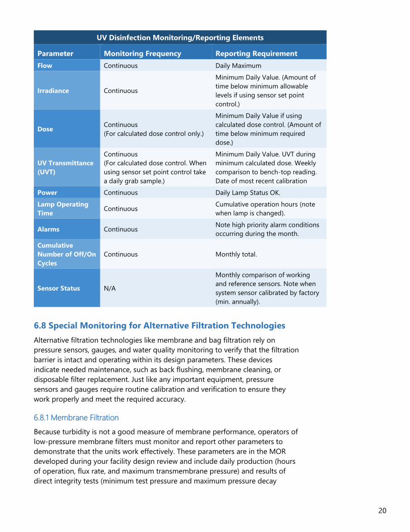
The MOR identifies specific parameters needed to monitor and confirm that the
reactor operates within validated conditions. The MOR also documents quality
assurance and quality control (QA/QC) procedures, such as calibration and
verification of UVT analyzers and sensors. The table below shows typical
monitoring and reporting parameters.
20
UV Disinfection Monitoring/Reporting Elements
Parameter Monitoring Frequency Reporting Requirement
Flow Continuous Daily Maximum
Irradiance Continuous
Minimum Daily Value. (Amount of
time below minimum allowable
levels if using sensor set point
control.)
Dose Continuous
(For calculated dose control only.)
Minimum Daily Value if using
calculated dose control. (Amount of
time below minimum required
dose.)
UV Transmittance
(UVT)
Continuous
(For calculated dose control. When
using sensor set point control take
a daily grab sample.)
Minimum Daily Value. UVT during
minimum calculated dose. Weekly
comparison to bench-top reading.
Date of most recent calibration
Power Continuous Daily Lamp Status OK.
Lamp Operating
Time Continuous
Cumulative operation hours (note
when lamp is changed).
Alarms Continuous Note high priority alarm conditions
occurring during the month.
Cumulative
Number of Off/On
Cycles
Continuous Monthly total.
Sensor Status N/A
Monthly comparison of working
and reference sensors. Note when
system sensor calibrated by factory
(min. annually).
6.8 Special Monitoring for Alternative Filtration Technologies
Alternative filtration technologies like membrane and bag filtration rely on
pressure sensors, gauges, and water quality monitoring to verify that the filtration
barrier is intact and operating within its design parameters. These devices
indicate needed maintenance, such as back flushing, membrane cleaning, or
disposable filter replacement. Just like any important equipment, pressure
sensors and gauges require routine calibration and verification to ensure they
work properly and meet the required accuracy.
6.8.1 Membrane Filtration
Because turbidity is not a good measure of membrane performance, operators of
low-pressure membrane filters must monitor and report other parameters to
demonstrate that the units work effectively. These parameters are in the MOR
developed during your facility design review and include daily production (hours
of operation, flux rate, and maximum transmembrane pressure) and results of
direct integrity tests (minimum test pressure and maximum pressure decay

21
(psi/min)). These requirements are in addition to combined filter effluent turbidity
measurements in the SWTR.
Direct integrity testing uses pressure decay testing (PDT) as the primary tool to
ensure membrane filters operate properly. You must complete PDT at least once
per day. There are specific PDT requirements for each membrane technology.
Pressure sensor calibration is an essential part of quality assurance. Calibrate
pressure sensors at least once per year, or more often if the manufacturer
recommends it, to ensure they continue to meet the accuracy specified in the
original design.
Indirect integrity testing uses particle counts or high-resolution turbidity (from
laser turbidimeters) continuously measured from each filtration unit (skid, cell, or
train). Systems must use indirect integrity testing to determine when they need to
run PDTs more often than once per day. You must report the daily maximum
value of the continuous readings (counts/mL or mNTU) on your MOR.
To calibrate and verify laser turbidimeters, follow procedures in Section 6.4.1.
Particle counters require regular maintenance, including cleaning and annual or
semiannual calibration. Follow your equipment manufacturer’s recommendations.
6.8.2 Bag and Cartridge Filtration
Bag and cartridge filtration systems use pressure gauges to determine when
filters need replacement. Giardia and Cryptosporidium filters have specific
maximum differential pressure limits of 20 to 30 psi based on their alternative
filtration technology approval. Make sure you measure pressure differentials at
the right location as shown in the table below.
Measure pressure differential with a single differential pressure gauge or separate
gauges on the inlet and outline lines. Check installed pressure gauges at least
once per year to ensure they read accurately. Keep several spare gauges on hand,
in case they need replacement. Quickly check a gauge by swapping it with a new
gauge and comparing the two readings. They should match within the accuracy
of the gauge, typically 2 to 3 percent of full scale.
Bag and Cartridge Filtration Pressure Differential Limits
Make/model Configuration Maximum Pressure
Differential (psi) How measured
Harmsco
HC/170-LT2 (filter)
MUNI-1-2FL-304 (housing)
Single filter
housing, multiple
cartridges
30 Absolute pressure
drop across the filter
Rosedale
PS-520-PPP0241 & GLR-PO-
825-2 (filters)
8-30-2P (housing)
Dual housings 20
Absolute pressure
drop across both
filters
Strainrite
HPM99_CC-2-SR & HPM99-
CCX-2-SR (filters)
AQ2-2 (housing)
Dual housings 25
Absolute pressure
drop across both
filters

22
7.0 Critical Alarms and Alarm Set Points
Critical alarms help ensure your disinfection and filtration processes are working,
there is neither too much nor too little water in the clearwell, and you are not
adding unsafe amounts of key water treatment chemicals. Focus on critical
treatment processes, such as coagulation, filtration, and disinfection, where
treatment failure poses an immediate risk to public health or safety.
Each treatment plant has a unique set of critical alarms. The most common are
turbidity, chlorine residual, pH, and clearwell level. The alarm settings must allow
a margin of safety so you have time to correct the problem or shut down the
process before a regulatory or health limit is reached. Typical alarm setpoints are
in Appendix A.12.
If your plant runs in unattended mode, critical alarms must trigger plant
shutdown, in addition to dialing out to the on-call operator.
Alarms and the callout systems they activate must be tested regularly so they will
function reliably when a problem occurs. For plants that run in unattended mode,
alarms must be tested at least monthly. For plants staffed 24/7, alarms should be
tested at least quarterly or at the same time as routine manufacturer-
recommended instrument calibration. Alarms and callouts should always be
tested following a power outage or after work is done on the system. Test even
more often if equipment is older or the plant has a history of problems.
Test alarms by checking set points at the instrument or in SCADA, injecting test
solutions or simulating a high reading. Allow the alarms to run long enough to
perform callouts, and verify the callouts are received by the intended phone
numbers. Consult the manufacturer for suggestions on the best way to test your
equipment. For example,
Alarm set points: Check the alarm settings at each on-line instrument. If
you have a SCADA system, check the settings in the control program by
checking each critical alarm against a master list from your written
Operations Program.
Chlorine residual: Shut off the flow in the sample line and inject an
unchlorinated or over-chlorinated test solution. Restore normal flow to
the instrument when finished.
Turbidity: Pull the head of the turbidimeters to simulate a high reading.
Lower the alarm set point to below the current reading until the alarm
triggers. Restore the set point when complete.
pH: Shut off the flow in the sample line and inject a high pH or low pH
test solution. Restore normal flow to the instrument when finished.
If an alarm fails and allows inadequately treated water to enter the system,
contact your regional office immediately to find out whether a health advisory or
other follow-up is needed. Conduct an after-incident review, correct any
deficiencies identified, and document lessons learned.

23
Review your plant’s standard operating procedures as discussed in section 8.0 to
make sure your customers are protected even when things go wrong. You can
find more information on alarms and alarm set points in these references:
1. Reliability for Filtered Systems, WAC 246-290-678.
apps.leg.wa.gov/wac/default.aspx?cite=246-290-678
2. AWWA Standard G100-11: Water Treatment Plant Operation and
Management. awwa.org/store/productdetail.aspx?productid=6923
3. Recommended Standards for Water Works. Policies for reviewing and
approving plans and specifications for public water supplies.
health.state.mn.us/communities/environment/water/tenstates/standards
8.0 Standard Operating Procedures
Written standard operating procedures (SOPs) help ensure every operator at your
facility follows consistent and correct procedures, your plant meets regulatory
requirements, and your utility follows best industry practices. Don’t make this
hard. Your SOPs should be short and simple, while still covering what’s important.
This makes them easier to create, update, and maintain. Review them at least
once per year and consider testing them whenever you train a new employee.
Critical SOPs for surface water treatment monitoring include procedures for
measuring chlorine, pH, and turbidity; instrument settings for online
turbidimeters; procedures for calculating inactivation ratio; and alarm setpoints
and testing. Use the sample SOPs for measuring pH, chlorine residual, and
turbidity in Appendix A.5 through A.8 as baseline documents, and tailor them to
your plant and your needs.
9.0 Recordkeeping and Reporting
You must maintain accurate and complete records of your surface water
treatment monitoring (WAC 246-290-639). You must record monitoring results
on ODW-approved forms and submit them to us by the tenth day of the
following month. Many of the more common forms are available at
doh.wa.gov/odwpubs.
Follow record management best practices. Records must be legible, readily
identifiable and retrievable. Avoid losing records to fire, flood, computer
malfunction, or other disaster by maintaining duplicate copies. Store duplicate
records in a secure, off-site location that’s easily accessible in a timely manner.
Automatic routine backups are best. Data log storage devices should have surge
protection and uninterruptible power supplies to avoid data loss during a power
surge or outage. Be sure to protect your data storage system against
unauthorized access.
Regulations set minimum record retention requirements for your facility (WAC
246-290-480). You must keep source meter readings for at least ten years,
turbidity data for at least five years, and most other plant monitoring and
performance data for at least three years.

24
Many treatment plants have a single logbook with handwritten notes about any
treatment plant activity. These logbooks are useful tools for operators, but
probably aren’t adequate for tracking and scheduling routine maintenance of
specific equipment or instrumentation. We recommend keeping individual
logbooks for each type of instrument, and recording all maintenance, calibration,
verification, and repair information in that logbook. This can be a physical book
or an electronic system, such as a database or spreadsheet, whatever works best
for your utility.
10.0 Conclusions
Quality data you can trust depends on proper installation and maintenance of
your equipment, robust calibration and verification procedures, and accurate
reporting. Qualified and certified operators make it happen by building and
sustaining a culture of excellence.
If you have questions about system-specific requirements for your utility or any
of the information in this document, contact your regional office.
Eastern Regional Office 509-329-2100
Northwest Regional Office 253-395-6750
Southwest Regional Office 360-236-3030

25
Appendix A.1 Sample SWTR Monitoring Plan (small slow sand plant)
A.2 Sample SWTR Monitoring Plan (rapid rate conventional plant)
A.3 Acceptable methods for measuring turbidity, temperature and pH
A.4 Acceptable methods for measuring residual disinfectant
A.5 Sample SOP: Measuring turbidity-Hach 2100Q Portable Turbidimeter (0-1000 NTU)
A.6 Sample SOP: Measuring free chlorine residual-Hach Pocket Colorimeter II (0.02 – 8 mg/L)
A.7 Sample SOP: Check of Chlorine Test Kit using Standard Additions-Pocket Colorimeter II
A.8 Sample SOP: Measuring pH using Hach SensION+ Portable Test Kit and 5050T probe
A.9 Recommended On-line Turbidimeter Settings and Monitoring Guidelines: Rapid Rate & Membrane
Filtration Plants
A.10 Recommended On-line Turbidimeter Settings: Unfiltered sources and Slow Sand, DE, and Bag
Filtration Systems
A.11 Plumbing Sample to a Process Analyzer—Thoughts to Ponder
A.12 Typical Alarm Set Points

26
A.1 Sample SWTR Monitoring Plan (Small Slow Sand Filter Plant)
Parameter Procedure Equipment
Filtration Process
Fecal coliforms
(raw)
Collect grab sample on first day of month from raw water sample tap
installed before slow sand filters. Mark sample lab slip as “Surface or GWI Raw
Source Water Sample”, check box labeled “Fecal,” Filtered “Yes,” and record
source ID “01.” When you receive results from lab, record fecal coliform count
on MOR summary page.
100 mL sample bottle (from
the lab)
Turbidity (raw) Collect grab sample each morning (daily) from raw water sample tap installed
before slow sand filters. Record value on MOR.
Hach 2100Q portable
turbidimeter
Turbidity filtered
(IFE)
An on-line instrument is connected to the filter effluent pipe of each slow
sand filter. Every morning, record displayed value from each instrument on
the MOR.
Hach 1720E/SC200
Turbidity filtered
(CFE)
An on-line instrument is connected to the combined filter effluent pipe prior
to the clearwell. Every morning record the value displayed on the instrument
on the MOR.
Hach 1720E/SC200
Disinfection: Inactivation Ratio Determination
Disinfection Sequence 1. Pipeline from treatment plant to storage tank. Assumed 1.0 baffling factor.
Temperature (ºC) Collect sample each morning from Ranger House kitchen sink (first service)
and immediately measure temperature.
Fischer Scientific digital
traceable thermometer
pH Collect sample each morning from Ranger House kitchen sink and
immediately measure pH.
Hach SensION portable with
5050T probe
Free Chlorine
Residual (mg/L)
Collect sample each morning from Ranger House kitchen sink and quickly
measure free chlorine residual. Hach Pocket Colorimeter II
Peak hourly flow,
PHF (gpm)
PHF is controlled by transfer pump rate from treatment plant to the 8,900-
gallon storage reservoir. Use constant rate of 3 gpm. Verify flow every year
using tank drawdown test.
Contact Time (min)
Contact volume based on 15 LF of 12-inch diameter pipe, followed by 290 LF
of 2-inch diameter pipe (134 gallons total) T=V/PHF=134÷3=44. Use
constant 44-minute time.
Disinfection Sequence 2. Unbaffled 8,900-gallon storage tank with separate inlet and outlet. Empirical 0.1 baffling factor.
Dimensions: 13 ft inside diameter, 9 ft maximum depth (pump-off setting).
Temperature, pH &
free chlorine residual Use same monitoring point for both sequences (see above) See above
Peak hourly flow,
PHF (gpm)
PHF is maximum one-hour flow leaving reservoir, expressed in gallons per
minute. Data logger captures hourly values from flow meter on reservoir
discharge. Every morning, record PHF for previous day.
Badger 2-inch positive
displacement meter with
data logger.
Reservoir depth, feet Record level each morning before plant start up External sight gauge
Contact Time (min) Daily calculation. Contact volume is based on recorded daily water depth
measurement, D, in feet. V=994 gal/ft x D. T=0.1 x V/PHF
Entry Point and Distribution Residual
Free Chlorine
Residual (mg/L)
(Entry point) Use same location as chlorine residual for CT. Population is <500
people, one grab sample per day is required Hach Pocket Colorimeter II
Free Chlorine
Residual (mg/L)
(Distribution) Collect a grab sample each morning from campground, rotating
among listed sites in coliform monitoring plan. Also, measure whenever
collecting a routine or repeat coliform sample.
Hach Pocket Colorimeter II

27
A.2 Sample SWTR Monitoring Plan (Rapid Rate Conventional Plant)
Parameter Process Equipment
Filtration Process
Turbidity (raw) Collect grab sample each morning (daily) from raw water tap, just inside
plant, prior to chemical injection. Record values on MOR. Hach 2100N
Turbidity (settled) An online instrument is connected to settled water effluent line. Values
sent to SCADA. Record average daily value on MOR.
Microtol 3/02055
Turbidity filtered
(IFE)
An online instrument is connected to effluent pipe from each filter.
SCADA historian records value every 15 minutes of operation Microtol 3/02055
Turbidity filtered
(CFE)
An online instrument is connected to combined filter effluent pipe prior
to clearwell via sample pump. Using SCADA trend, report values 15
minutes after plant startup and subsequent readings every 4 hours on
MOR. Report absolute max. for day from SCADA trend chart.
Microtol 3/02055
Disinfection: Inactivation Ratio Determination
One disinfection sequence: 100,000 gallon baffled reservoir. 0.35 baffling factor from 2016 tracer study. Dimensions: 29 ft inside
diameter, 17 ft maximum depth (overflow).
Temperature (ºC) Collect grab sample twice daily from tap on discharge side of high
service pump (clearwell effluent). Report min. of two values on MOR.
Fischer Scientific digital traceable
thermometer
pH Collect grab sample two times daily from tap on discharge side of high
service pump (clearwell effluent). Report max. of two values on MOR. Hach HQ 30D
Free chlorine
residual (mg/L)
Measured continuously from sample tap on discharge side of high
service pump (clearwell effluent). Report daily min. value from SCADA
trend on MOR.
Cl-17 (continuous), DR890 (grab)
Peak hourly flow,
PHF (gpm)
Measured continuously by flowmeter on tank effluent line. Values sent
to SCADA every minute. SCADA calculates max. one-hour flow leaving
reservoir each day, expressed in gallons per minute. Record on MOR.
Allen Bradley magmeter,
recorded to SCADA
Tank Depth (ft) Measured continuously, values sent to SCADA every minute. Record
lowest daily level from SCADA on MOR.
Pressure transducer, recorded to
SCADA
Contact Time (min) Calculate daily. Contact volume based on recorded daily water depth
measurement, D, in feet. V=4900 gal/ft x D. T=0.35 x V/PHF
Entry Point and Distribution Residual
Free chlorine
residual (mg/L)
(Entry point) Measured continuously. Use same location as chlorine
residual for CT. Report min. daily value on MOR. Cl-17 (continuous), DR890 (grab)
Free chlorine
residual (mg/L)
(Distribution) Collect at least one grab sample every day rotating among
sites in coliform monitoring plan. Also, measure whenever collecting
routine or repeat coliform sample.
DR890
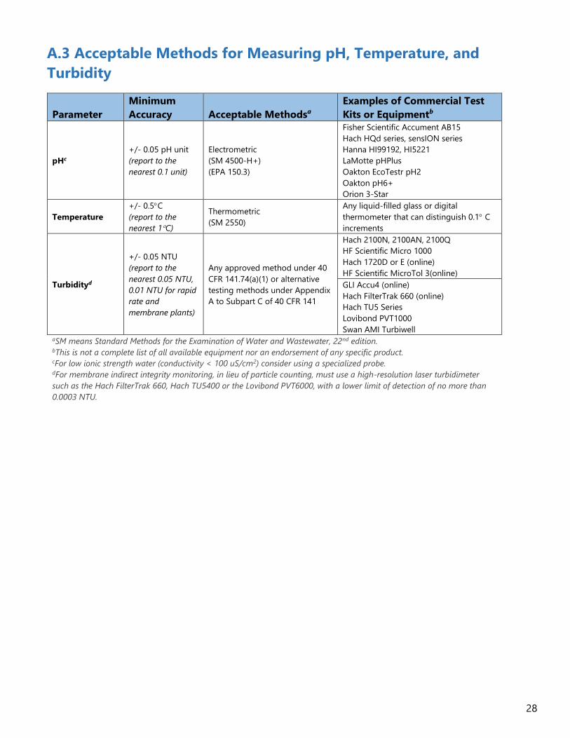
28
A.3 Acceptable Methods for Measuring pH, Temperature, and
Turbidity
Parameter
Minimum
Accuracy Acceptable Methodsa
Examples of Commercial Test
Kits or Equipmentb
pHc
+/- 0.05 pH unit
(report to the
nearest 0.1 unit)
Electrometric
(SM 4500-H+)
(EPA 150.3)
Fisher Scientific Accument AB15
Hach HQd series, sensION series
Hanna HI99192, HI5221
LaMotte pHPlus
Oakton EcoTestr pH2
Oakton pH6+
Orion 3-Star
Temperature
+/- 0.5C
(report to the
nearest 1C)
Thermometric
(SM 2550)
Any liquid-filled glass or digital
thermometer that can distinguish 0.1 C
increments
Turbidityd
+/- 0.05 NTU
(report to the
nearest 0.05 NTU,
0.01 NTU for rapid
rate and
membrane plants)
Any approved method under 40
CFR 141.74(a)(1) or alternative
testing methods under Appendix
A to Subpart C of 40 CFR 141
Hach 2100N, 2100AN, 2100Q
HF Scientific Micro 1000
Hach 1720D or E (online)
HF Scientific MicroTol 3(online)
GLI Accu4 (online)
Hach FilterTrak 660 (online)
Hach TU5 Series
Lovibond PVT1000
Swan AMI Turbiwell aSM means Standard Methods for the Examination of Water and Wastewater, 22nd edition. bThis is not a complete list of all available equipment nor an endorsement of any specific product. cFor low ionic strength water (conductivity < 100 uS/cm2) consider using a specialized probe. dFor membrane indirect integrity monitoring, in lieu of particle counting, must use a high-resolution laser turbidimeter
such as the Hach FilterTrak 660, Hach TU5400 or the Lovibond PVT6000, with a lower limit of detection of no more than
0.0003 NTU.

29
A.4 Acceptable Methods for Measuring Residual Disinfectant
Parameter
Minimum
Accuracy Acceptable Methodsa
Examples of Commercial
Test Kits or Equipmentb,c
Free chlorined
+/- 0.1 mg/L
(report to the
nearest 0.1 mg/L)
Amperometric titration (SM 4500
Cl-D)
DPD-ferrous titration (SM 4500
Cl-F)
DPD-colorimetric (SM 4500 Cl-G)
Hach Pocket Colorimeter II
Hach DR 890/900
LaMotte DC-1500CL
LaMotte SMART Colorimeter
Hach Cl-17 (online)
Syringaldizine (FACTS) (SM 4500
Cl-H)
EPA 334.0 Any online analyzer
Combined chlorined
(chloramines) +/- 0.1 mg\/L
Amperometric titration (SM 4500
Cl-D and 4500 Cl-E)
DPD-ferrous titration (SM 4500
Cl-F)
DPD-colorimetric (SM 4500 Cl-G)
Hach Pocket Colorimeter II
Hach DR890/900
Hach Cl-17 (online)
Iodometric electrode (SM 4500
Cl-I)
EPA 334.0 Any online analyzer
Chlorine dioxide +/- 0.05 mg/L
DPD Method (SM 4500-Cl02D) Hach DR900, DR1900
Amperometric titration (SM 4500-
Cl02 C, 4500-Cl02 E)
Spectrophotometric (EPA 327.0)
Amperometric sensor ChloridoX Plus
Ozone +/- 0.02 mg/L Indigo method (SM 4500-O3B) Hach DR900, DR1900
Hach Pocket Colorimeter-ozone
a SM means Standard Methods for the Examination of Water and Wastewater, 22nd edition. b This is not a complete list of all available equipment nor an endorsement of any specific product c Color comparator test kits, such as color wheels & test strips are not acceptable for SWTR monitoring d Total chlorine minus free chlorine

30
A.5 Sample SOP: Measuring Turbidity—Hach 2100Q Portable
Turbidimeter (0–1000 NTU)
Method Summary, Instructions, Interferences and Tips
Turbidity is a measurement of scattered light from suspended solids: the higher the intensity of scattered light, the higher the
turbidity.
The HACH 2100Q measures turbidity in nephelometric turbidity units (NTU) using a nephelometric method that relies on passing
specific light at a specific wavelength through the sample.
Fine air bubbles can cause high readings. To reduce, allow the sample to sit for a few minutes to allow bubbles
to dissipate or use a syringe to apply a vacuum for 10 seconds.
Floating debris and coarse sediments, which settle out rapidly, will give low readings. If measuring raw or
settled water with higher turbidity, mix the sample to disperse the solids thoroughly. Wait until air bubbles
disappear then gently agitate the sample to resuspend any heavier particles without introducing air bubbles.
Condensation on the outer surface of sample cuvettes can cause erratic readings. Remove condensation by
coating the outside of the cuvette with a small amount of silicon oil and wiping thoroughly with a fresh lab
wipe. In cold weather, it may be necessary to move the turbidimeter indoors to measure sample turbidity;
allow samples to come to room temperature before analysis.
The presence of true color will cause readings to be low. True color is due to dissolved substances that absorb
light. Light absorbing materials, such as activated carbon in significant concentrations, can cause low readings.
Replace sample cuvettes when they become scratched or etched. You may use a light coating of silicon oil to
mask minor imperfections. Wipe thoroughly with a fresh lab wipe before reading the sample.
For improved accuracy, index each sample cuvette by filling it with deionized water, inserting it into the
turbidimeter, and rotating the cuvette to find the orientation that produces the lowest turbidity reading. Mark
the cuvette where it aligns with the raised orientation mark on the optical well of the turbidimeter. When
measuring the turbidity of a sample, align the mark on the cuvette with the raised orientation mark on the
meter.
Replace calibration and verification standards before they reach the expiration date on the label.
Calibration
Calibrate HACH 2100Q meter at least every three months and whenever verification does not pass. Use sealed StablCal formazin
solutions and follow directions on page 10 of HACH 2100Q Basic User Manual.
Use extreme care when handling Reference Standards and handle them by the top only. Surface scratches or finger smudges
cause analysis errors.

31
Measuring a Sample
1. Turn on meter. Invert 10 NTU Reference Standard several times until it is well mixed and place it into optical well with
orientation mark aligned with raised orientation mark in front of cell compartment (see page 10 of HACH 2100Q Basic User
Manual). Press “verify cal” and then “Read.” If the meter displays “Calibration Verification Passed,” meter is ready for use. If
not, recalibrate meter.
2. Start with a clean, indexed sample cuvette. Rinse it three times with sample water then fill to within about ½-inch of the top
with a sample directly from the sample tap. Place cap on sample cuvette and carefully wipe any condensation from outside
of the cuvette with a lint free lab wipe. Place sample cuvette into well, align index mark with raised orientation mark on
optical well, and press “Read.” Read NTU reading directly from the display. Record value to nearest recommended NTU (see
table below) on your field data sheet.
3. Rinse sample cuvette three times with deionized water to get it ready for the next sample.
4. Fill recently cleaned cuvettes with deionized water and store them in a manner to avoid contamination of the inside with
particles or scratches and abrasions to the outside surface.
5. Report results as follows.
NTU Reading Record to Nearest
0.0–1.0 0.05* *Rapid rate and membrane plants report to nearest 0.01.
1–10 0.1
10–40 1
40–100 5
100–400 10
400–1000 50
>1000 100
References
HACH. 2013. HACH 2100Q and 2100Qis Basic User Manual. HACH, Inc. Loveland, CO.
U.S. Environmental Protection Agency. 1993. Determination of Turbidity by Nephelometry. Method 180.1. Environmental Monitoring
and Support Laboratory, Cincinnati, OH.
U.S. Geological Survey. 1998. National Field Manual for the Collection of Water Quality Data. Book 9, Handbooks for Water-Resource
Investigations. United States Geological Survey. Reston, VA
Revision date: April 25, 2019.

32
A.6 Sample SOP: Measuring Free Chlorine Residual—Hach Pocket
Colorimeter II (0.02-8 mg/L)
General instructions Revision date: April 25, 2019.
Once per quarter, use standard additions to validate test procedure, reagents and
instrument (see separate SOP).
Once per week, measure SpecCheck® secondary standards (make sure not expired).
Use separate sample cells for free and total chlorine; caps are labeled “free” and “total.”
Use same sample cell for zeroing the instrument and taking a measurement.
For distribution samples, flush 5 minutes or as needed to get a sample from water main.
Low range (0.02 to 2 mg/L)
1. Turn on instrument and confirm it is in low range mode (LR)a.
2. Rinse sample cell and cap at least 3 times with water you will sample.
3. Fill sample cell to 10 mL line and replace cap. (Bottom of meniscus just above or touching the line).
4. Gently wipe cell clean and dry with a lab wipe.
5. Place sample cell in instrument with diamond facing instrument keypad.
6. Close cover securely, press blue “zero” button and wait for display to read 0.0.
7. Add contents of one 10 mL free chlorine residual reagent packet.
8. Replace cap and swirl for 20 seconds.
9. Wipe cell dry with a lab wipe.
10. Immediatelyb insert cell into instrument with diamond facing keyboard.
11. Close instrument cover securely and press green “read” button.
12. Important! Rinse sample cell thoroughly after use and allow it to air dry if possible.
High range (0.1-8 mg/L)c
1. Use plastic high-range sample cell.
2. Turn on the instrument and confirm it is in the high range mode (HR)a.
3. Rinse sample cell and cap at least 3 times with water you will sample.
4. Fill sample cell to the 5 mL line and replace the cap. (Bottom of meniscus just above or touching the line).
5. Wipe cell clean and dry with a lab wipe.
6. Place cell in instrument with diamond facing the instrument keypad.
7. Close cover securely, press “zero” button and wait for display to read 0.0.
8. Add contents of two 10 mL free chlorine residual reagent packets.
9. Replace cap and swirl for 20 seconds.
10. Immediatelyb insert cell into the instrument with diamond facing the keyboard.
11. Close cover securely and press green “read” button.
12. Important! When done testing, rinse sample cell thoroughly and allow it to air dry, if possible.
aTo switch between high range (HR) and low range (LR), press menu button, then blue zero button until display reads SEL. Press
green button to toggle between LR and HR. Press menu button again to exit. bCaution! Time from adding the reagent to reading the result must not exceed 1 minute. cIf chlorine concentration is typically less than 2 mg/L, use low range procedure.
Revision date: April 25, 2019.

33
A.7 Sample SOP: Check of Chlorine Test Kit Using Standard
Additions-Pocket Colorimeter II
Purpose: Evaluate your chlorine testing equipment and techniques to verify testing accuracy and precision.
Equipment and supplies: Hach Pocket Colorimeter II® with 10 mL sample cuvette, chlorine standard solution (25-
30 mg/L, 2 mL ampules), ampule breaker, small Tensette® pipet (0.1-1.0 mL) and disposable tips, large Tensette®
pipet (1-10 mL) and disposable tips, free or total chlorine reagent, SpecCheck® secondary standard.
Procedure
1. Rinse cuvette with deionized water 4–5 times. Shake with the cap on.
2. Shake out all the water.
3. Measure 10 mL deionized water with the large pipet1 and dispense it into the cuvette.
4. Add a powder pillow (either total or free), swirl to mix. Wipe the outside of the cuvette with a lab wipe.
5. Insert the cuvette into the instrument. Orient the cell alignment mark facing towards the keypad.
6. Zero the instrument. This corrects for color and turbidity of sample and reagent.
7. Get the small pipet1 ready. Measure 0.1 mL of the standard. Waste the first dose.
8. Dispense the standard into the cuvette, swirl to mix.
9. Read the sample and record the results in the data table below.
10. Repeat steps 7–9 at least four times.
11. Calculate percent recovery of the test samples and compare to the concentration you expected (see data table below).
1Pipet Tips (Tensette® pipet)
Make sure the tip is on snugly.
Use the alignment mark.
Push the plunger down before putting the tip in the liquid.
Once in the liquid, raise your thumb slowly.
Before dispensing the liquid, click to the next highest number (for max value use “F”) (Note: some pipette brands have
two stops. If your pipette has two stops, skip this step).
Dispense “with gusto,” keeping the tip of the pipette above the liquid.
Troubleshooting tips if results show greater than 10 percent variance.
Try a reagent with a different lot number.
Clean the vial or try a new vial.
Verify that the primary standard is not expired.
Verify the calculation for expected concentration and percent recovery.
Have another individual go through the procedure with the same equipment.
Verify the volume the pipette delivered. The density of water is 1 gram/mL. You can test the volume delivered by
weighing it with a laboratory scale.
Ref: Hach Method 8021, Free Chlorine, Doc316.53.01023
Revision date: April 25, 2019.

34
Example Standard Additions Data Table
Test kit
Make/Model Hach Pocket Colorimeter II
Serial
Number 0E26279
Manufacturer’s
estimated detection
limit, mg/L
0.02 Analyst/User BC
Chlorine standard
concentration, Cs,
mg/L
25.6 Date 6/12/2017
Sample # Sample
vol (mL)
Expected
Concentration,
C’
Measured
Values
(mg/L)
% Recovery Notes
blank 10.0 0.00 Original sample, C0
1 10.1 0.253 0.26 103 Added 0.1 ml solution
2 10.2 0.502 0.50 100 Added 0.1 ml solution
3 10.3 0.746 0.75 101 Added 0.1 ml solution
4 10.4 0.985 0.97 99 Added 0.1 ml solution
o.k. Acceptable performance, 100
+/-10%
C1V1=C2V2: C’ = Cs(mL std added)/(10+(0.1)(# of additions))
% Recovery = (Measured Value/C’) x 100

35
A.8 Sample SOP: Measuring pH Using Hach SensION+ Portable Test
Kit and 5050T Probe
General instructions
Calibrate instrument using pH 4, 7 and 10 buffers each day you use it. Follow instructions in case. Record slope and
offset, and confirm they are within acceptable limits.
slope=-59.14 (+/- 5%); offset=0 +/- 30 mV
Refrigerate buffers and replace before expiration date. Before using, allow buffers to warm up to temperature of water
to be tested.
Verify instrument using a pH 6.85 or 8 buffer before each set of readings.
Sample from a smooth, pencil-sized stream, taking care not to aerate sample.
Air bubbles trapped under the probe tip cause errors. If present, gently shake the probe until bubbles are removed.
Store probe in KCl solution when finished sampling for the day. For storage, orient case so probe tip is pointing down
(tip immersed in storage solution).
Calibrate the meter
1. Fill each labeled buffer tube with appropriate pH buffer. Fill DI bottle.
2. Remove probe from storage solution and rinse with DI water. Blot dry with lab wipe, making sure to dab the tip of the
electrode carefully.
3. Place electrode in the pH 4 buffer. Turn on unit.
4. Press [••• button to make sure meter is set to pH mode. Press [••• again to accept parameter and press a third time to
read buffer. Wait until screen indicates meter is ready for next pH buffer.
5. Rinse pH probe with DI water in between buffers and dab with lab wipe.
6. Repeat with pH 7 and 10 buffers.
7. Perform a verification check with another buffer (pH 6.85 or 8).
8. Empty the pH buffer tubes at the end of each day.
Taking a reading
1. Rinse probe with DI water. Blot dry with lab wipe.
2. If not already done, verify calibration using a fresh pH 6.85 or 8 buffer (single point). If not within +/-0.2 units of true
value, recalibrate.
3. Allow probe to sit in sample water for five minutes.
4. Collect fresh sample and insert probe.
5. While gently swirling, press read button and allow reading to stabilize.
6. Record pH, temperature, and time of measurement.
7. Wait several seconds and press read again. Ideally, pH and temperature will stay the same (+/- 0.05 units).
Revision date: April 25, 2019

36
A.9 Recommended On-line Turbidimeter Settings and Monitoring
Guidelines: Rapid Rate and Membrane Filtration
Turbidimeter Setting or
Activity Recommendation Comments
Sample Flow Rate Measure at least monthly. Meet
the manufacturer’s specifications.
For the 1720E, a flow rate of 500 ml/min appears to be a
good starting point (Hach specifies 200 to 750 ml/min).
Higher flow rates will provide a quicker response time, but
may cause problems with air bubbles in cold temperatures.
For TU5 models manufacturer recommends flow rate of
200 mL/min when the maximum particle size is 20 μm. For
larger particles (150 μm maximum), increase flow rate to
350 to 500 mL/min.
Error Hold Mode
The output should be set to
“Transfer” mode with a transfer
setting of 0.0 NTU.
When a controller loses communication with its sensor, it
either holds the output at the last good reading or
transfers to a predefined value. (The Hach SC controller
default setting is HOLD.) The HOLD mode makes it more
difficult to detect a communication anomaly because it
holds the last measurement. When the TRANSFER mode is
active, the controller will report a turbidity of 0.0 NTU,
which would prompt the operator to investigate further.
Signal Averaging 30 seconds
The purpose of this setting is to achieve a stable turbidity
reading for identifying trends. Too short of a setting may
not provide a stable reading if the instrument becomes too
sensitive to individual particles. A longer period will result
in slower response times and may miss turbidity spikes.
Bulb Replacement At least annually or as the
manufacturer recommends.
For units with incandescent bulbs. Failing bulbs can cause
the turbidimeter to lose its quarterly calibration.
Signal Span (Minimum and
Maximum) Data Capping 0–5 NTU for finished water.
These settings do not affect the turbidity value displayed
locally on a Hach turbidimeter or controller, but they will
cap the data sent to the SCADA system or to an attached
recorder. For example, using a 4–20 mA signal, if 20 mA
equates to 1.0 NTU, then the controller will not send any
turbidity value over 1.0 NTU to SCADA. The signal span
maximum value must be set above the regulatory limit for
that monitoring location. The CFE turbidimeter must be
able to measure and record turbidities exceeding 1.0 NTU
and IFE turbidimeters must be able to measure and record
turbidities exceeding 2.0 NTU.
SCADA/Data recorder Required. Must match the
turbidimeter reading.
The data recorder/SCADA must be scaled to match the
turbidimeter signal span.
Bubble Reject On Bubbles are “noise” and will cause turbidity spikes.
Sensor Datalog Interval (If
No SCADA or Recorder)
1 or 5 minutes (1 min is preferred
unless data storage or processing
limitations exist).
If set to 15 minutes, this will store about 6 months of data,
and can be a backup to your primary recording system.
Cleaning Interval (TU5
models) 12 hours (default)
For units equipped with automatic cleaning module
(recommended). Adjust this based on water quality and
plant experience. Daily cleaning may be sufficient for high
quality filtered water.

37
A.10 Recommended On-Line Turbidimeter Settings
Unfiltered Sources and Slow Sand, DE and Bag Filtration Plants
Turbidimeter Setting
or Activity Recommendation Comments
Sample Flow Rate Measure at least monthly. Meet
the manufacturer’s specifications.
For the 1720E, a flow rate of 500 ml/min is a good starting point
(Hach specifies 200 to 750 ml/min). Higher flow rates provide a
quicker response time but may cause problems with air bubbles
in cold temperatures. For TU5 models manufacturer
recommends flow rate of 200 mL/min when the maximum
particle size is 20 μm. For larger particles (150 μm maximum),
increase flow rate to 350 to 500 mL/min.
Error Hold Mode
You should set the output to
“Transfer” mode with a transfer
setting of 0.0 NTU.
When a controller loses communication with its sensor, it either
holds the output at the last good reading or transfers to a
predefined value. (The Hach SC controller default setting is
HOLD.) The HOLD mode makes it more difficult to detect a
communication anomaly because it holds the last measurement.
When the TRANSFER mode is active, the controller will report a
turbidity of 0.0 NTU, which would prompt the operator to
investigate.
Signal Averaging 30 seconds
The purpose of this setting is to achieve a stable turbidity
reading for identifying trends. Too short a setting may not
provide a stable reading if the instrument becomes too sensitive
to individual particles. A longer time will result in slower
response times and may miss turbidity spikes.
Bulb Replacement At least annually or as the
manufacturer recommends.
For units with incandescent bulbs. Failing bulbs can cause the
turbidimeter to lose its quarterly calibration.
Signal Span (Minimum And
Maximum) Data Capping 0–10 NTU for finished water.
These settings do not affect the turbidity value displayed locally
on a Hach turbidimeter or controller, but they will cap the data
sent to the SCADA system or to an attached recorder. For
example, using a 4–20 mA signal, if 20 mA equates to 1.0 NTU,
the controller will not send any turbidity value over 1.0 NTU to
SCADA. The signal span maximum value must be set above the
regulatory limit for that monitoring location. The CFE
turbidimeter must be able to measure and record turbidities
over 5.0 NTU
Data Recorder or SCADA Required. Must match
turbidimeter reading.
The data recorder or SCADA must be scaled to match the
turbidimeter signal span.
Bubble Reject On Bubbles are “noise” and will cause turbidity spikes.
Sensor Datalog Interval (If
No SCADA or Recorder)
1 or 5 minutes (1 min is
preferred unless data storage or
processing limitations exist).
If set to 15 minutes, this will store about 6 months of data, and
can be a backup to your primary recording system
Cleaning Interval (TU5
models) 12 hour (default)
For units equipped with automatic cleaning module
(recommended). Adjust this based on water quality & plant
experience. Daily cleaning may be sufficient for high quality
filtered water.

38
A.11 Plumbing Sample to a Process Analyzer—Thoughts to Ponder
Terry Engelhardt, Application Development Manager—Drinking Water, Hach Company
Location, Location, Location—If The Sample Is Not Right The Analysis Is Not Right!
1. Is the sample well mixed and representative?
a. Any chemical addition which can affect the measurement should be added far enough ahead of the
sample point that it is well mixed and in solution. For example, if pH is to be measured after lime is
added for pH adjustment, the measurement needs to be made far enough downstream that all the
lime is in solution.
b. If a chemical addition will interfere with measurement of the parameter of interest, the sample
should be drawn before the point of chemical addition. For example, suspended lime particles can
cause positive error in particle count measurements following filtration. Measure particle counts in
filter effluent prior to lime addition.
2. Where possible avoid turbulent flow conditions—i.e., sample locations near valves, ells, tees, flanges.
Turbulent flow conditions may dislodge scale, introduce severe entrained air and cause other sample
anomalies, which will lead to inaccurate measurement.
Keep It Short, Keep It Simple, And Don’t Delay
1. The instrument should be located as close as is practical to the sample location. If the sample to be
measured is in the pipe gallery, then the instrument should be there too! Avoid piping sample long
distances. Exceptions to the ‘keep it short’ rule include—
a. Do not mount instruments in locations where the environment will be hostile to the function and life
of the instrument, i.e. areas with corrosive gases or strong electromagnetic fields.
b. Do not mount instruments in locations that are hazardous or difficult to access for operations and
maintenance personnel. All instruments require periodic maintenance. If instruments are difficult or
hazardous to access to perform required maintenance, they won’t be maintained and they won’t
work!
2. Use sample lines that are corrosion resistant, small diameter and maintain high sample velocity
a. Where possible use opaque, black plastic or metallic pipe/tubing compatible with the sample to be
measured. The sample line must be opaque to block all light thus discouraging biofilm.
b. Use the smallest diameter tubing that will deliver adequate volume and maintain high velocity.
i. Select small diameter sample line to minimize the volume contained in the sample line and to
maintain a high velocity.
ii. Maintaining high velocity in the tubing will discourage accumulation of biofilm and solids, which
will affect accuracy.
c. Don’t delay—Keep it short, keep it simple, maintain high velocity. See “Sample Delay” table.
Do Not Mix and Match Plumbing Fittings!
1. Do not come off a steel pipe with a galvanized nipple, connected to a brass valve, which will then
connect to a copper sample line before getting to the analyzer. This is all too common and creates a
galvanic corrosion cell at every point of contact between dissimilar metals.
2. Get to corrosion resistant materials as quickly as possible with minimal changes in the composition of
materials of the plumbing fittings. Preferably, install corrosion-resistant metal or plastic materials.

39
Go With the Flow—Every Place
for a Valve and Every Valve in its
Place
1. Controlling flow and pressure
is important for all
measurements, critical for
others. Instruments such as
amperometric chlorine
analyzers, particle counters and
turbidimeters are very sensitive
to changes in flow and
pressure
2. Valves—so many choices. Ball
valves, needle valves, gate
valves, globe valves
a. Needle valves—avoid. Needle valves typically are incorporated with rotameters. Seems simple,
measure flow and control flow all in one. Just say no!
i. Use a rotameter to measure flow if you wish. They are simple, easy to install and provide sufficient
accuracy.
ii. Do not use rotameters with integral needle valves for flow control. Needle valves create air
bubbles and easily become fouled with solids carried in the sample stream and corrosion
products that may slough off of plumbing fittings.
b. Ball and gate valves are commonly used to throttle (control) flow but they are not designed for flow
control. Use ball and gate valves for on/off control. Ball valves are convenient in that they are
normally ¼ turn from closed to fully open making operation fast and easy.
c. Globe valves are designed to control flow. Use globe valves to control flow to instruments.
Keep it right down the middle
1. Avoid sampling from the top or bottom of a pipe. Sampling from the top will often result in problems
with air in the sample. Sampling from the bottom will be non-representative due to solids, which will
inevitably accumulate at the bottom of the pipe.
2. Typically it is best to sample from the side of a pipe ± 45°.
3. It is desirable to sample from the middle of the pipe rather than from the edge,
especially on larger diameter pipe (say, 6” diameter or larger). Samples drawn from
the edge of a pipe can be non-representative due to fouling from sediment/biofilm
accumulated on the wall of the pipe.
4. Sample probes or sample quills are available from a number of manufacturers.
Some of these are fixed in place, others are retractable. The probes/quills are
available in a variety of materials. The probe pictured at right is retractable. And, it
has multiple ports so the sample is a cross section of the pipe rather than one point;
a feature may be desirable in some instances, especially larger diameter pipes.

40
Pump It Up—Or Not
1. Avoid pumping sample where possible.
Pumping can change the sample by
entraining air, changing sample temperature
(thus changing solubility of some
substances) contributing corrosion products
and/or changing the nature (i.e. size or
shape) of suspended material.
2. When pumping is unavoidable:
a. Avoid pumps which cause pulsation
(diaphragm, piston, and peristaltic
pumps). Pulsations can cause
measurement irregularity. If unavoidable,
use a pulse dampener after the pump.
b. Centrifugal pumps are typically preferred
to positive displacement pumps for
providing samples to analyzers due to
lower cost and centrifugal pumps are
easier to throttle (control flow and
pressure).
c. Select a pump with components
compatible with the sample. A pump with all composite (nonmetallic) wetted parts is desirable.
Pumps with metallic wetted parts can create measurement errors by introducing corrosion products.
d. Avoid excessive suction lift. At sea level, an ideal pump has a maximum lift of about 34 feet.
Considering pump efficiencies, and other factors, even at sea level, the practical suction lift is only
about 25ft. At a mile above sea level (Denver, Colorado) the practical lift of only about 21 feet. Pump
manufacturers will typically specify the maximum lift for their pump. Operating a pump near suction
lift design limits will cause cavitation and other problems. The suction side of a centrifugal pump
should not be restricted—the valve on the suction side should always be fully open. Where suction
lift is too great, one should consider a submersible pump.
When good sampling practices are not followed, don’t blame inaccurate measurement on
the instrument! If the sample is not right the analysis is not right!

41
A.12 Typical Alarm Set Points Type of
Plant/Parameter High/Low Purpose Typical Set Points
All Plants
Chlorine Residual Low-low
(shutdown)
Keep inadequately disinfected
water from entering the
distribution system.
Treatment plant specific.
As needed to maintain
IR above 1.0 and
chlorine at entry above
0.2 mg/L. Likely be 0.2
to 0.6 mg/L.
High-high
(shutdown)
Avoid exceeding the maximum
residual disinfectant level (MRDL).
Can be set as high as 4.0
mg/L, but should be
lower.
pH Low-low
(shutdown)
Detect an overfeed. Used only if
an acid is fed.
pH of 5.5 to 6.0 could be
used in most situations.
High-high
(shutdown)
Prevent high pH water from
entering the distribution system.
Used only if strong base is fed.
pH 9.0 to 9.5 could be
used in most situations.
Clearwell Level Low Avoid inadequately disinfected
water (IR<1.0) from entering the
distribution system.
Unique for each system.
As needed to maintain
IR above 1.0.
High-high
(shutdown)
Prevent an overflow that could
damage the plant.
Unique for each system.
Rapid Rate Filtration
Turbidity (combined
filter effluent)
High Alert the operator of a significant
process change so corrective
action can be taken.
0.10 NTU or slightly less.
High-high
(shutdown)
Avoid a treatment technique
violation.
Slightly less than 0.30
NTU.
Turbidity (individual
filter effluent)
High Maintain optimized performance.
End the filter run on turbidity
breakthrough.
0.10 NTU or slightly less

42
Membrane Filtration
Pressure decay test
(psi/min)
High Ensure the membranes are intact
and providing effective treatment
Use direct integrity upper
limit from alternative
technology memo.
Turbidity (combined
filter effluent)
High Avoid a treatment technique
violation.
Less than 0.10 NTU.
Turbidity or particle
counts (individual filter
effluent)
High Trigger a direct integrity test. Use indirect integrity
control limits from
alternative technology
memo.
Other filtration
technologies
Pressure differential
(bag filtration)
High Ensure the bags are not operated
outside their approved design.
Use maximum pressure
differential from
alternative technology
memo.
Filter flow rate (DE) Low Maintain integrity of the DE filter
cake.
Unique for each system.
Raw water turbidity (DE,
bag, slow sand)
High Prevent high turbidity raw water
from exceeding treatment plant
capability.
Unique for each system.
UV disinfection
UV Intensity Low, or
complete
outage
Ensure adequate UV lamp output
to provide the required dose
Unique for each system,
based on validated range
for the UV reactor
UV dose Low Ensure reactors are providing the
minimum required dose
UV transmittance Low Confirm operation within the
validated range for the reactor
Lamp breakage1 Limit mercury release (triggers
lamp breakage response plan)
Flowrate High Ensure reactor not operated
above the maximum approved
flowrate
1 Parameters monitored to detect lamp breakage vary by system.

43
References
ANSI/AWWA G100-17, Water Treatment Plant Operation and Management.
AWWA G200-15, Distribution System Operation and Management.
AWWA G400-09, Utility Management System.
AWWA Manual M6, Water Meters-Selection, Installation, Testing and Maintenance.
AWWA Manual M33, Flowmeters in Water Supply.
Deem, S. & Feagin, N., 2016. "Disinfection Data Integrity in Washington State." Journal AWWA, 108:10:24,
http://dx/doi/org/10.5942/jawwa.2016.108.0162.
Deem, S. & Feagin, N., 2014. "A Turbidity Data Verification Project in Washington." Journal AWWA 106:12:32,
http://dx/doi/org/10.5942/jawwa.2014.100.0162.
Engelhardt, T. & Malkov, V., 2015. “Plumbing Sample to a Process Analyzer.” Chlorination, Chloramination and Chlorine
Measurement, Appendix C. Hach Company, Loveland.
Incontri, Joe. “Flow Data Red Flags: When to Act.” Water Online, December 20, 2017.
Malkov, Vadim B. et. al., 2009. “Comparison of On-line Chlorine Analysis Methods and Instrumentation Built on
Amperometric and Colorimetric Technologies. Proceedings, AWWA Water Quality Technology Conference & Exposition
(Nov. 15–19, 2009), Seattle, Wash.
Standard Methods for the Examination of Water and Wastewater, 2012 (22nd ed.). APHA, AWWA, and WEF,
Washington.
USEPA (US Environmental Protection Agency), 1999. Alternative Disinfectants and Oxidants Guidance Manual. USEPA,
Washington.
USEPA (US Environmental Protection Agency), 1991. Guidance Manual for Compliance with the Filtration and
Disinfection Requirements for Public Water Systems Using Surface Water Sources. USEPA, Washington.
USEPA (US Environmental Protection Agency), 2005. Membrane Filtration Guidance Manual. USEPA, Washington.
USEPA (US Environmental Protection Agency), 2017. Method 150.3: Determination of pH in Drinking Water. USEPA,
Washington.
USEPA (US Environmental Protection Agency), 2009. Method 334.0: Determination of Residual Chlorine in Drinking
Water Using an On-line Chlorine Analyzer. USEPA, Washington.
USEPA (US Environmental Protection Agency), 2004. Preventative Maintenance Card File for Small Public Water
Systems Using Ground Water. USEPA, Washington.
USEPA (US Environmental Protection Agency), 2006. Ultraviolet Disinfection Guidance Manual for the Final Long Term 2
Enhanced Surface Water Treatment Rule. USEPA, Washington.
USEPA (US Environmental Protection Agency), 2019. Generating High-Quality Turbidity Data in Drinking Water
Treatment Plants to Support Optimization and Monitoring. USEPA, Washington.
Van Arsdel, John H., 2017. “Accurate Water Audits Require Accurate Master Meter Calibration and Testing.” Opflow
43:2. American Water Works Association, Denver.
WSDOH, 2019. “Appendix I: Ultraviolet Disinfection for Drinking Water Applications,” Water System Design Manual.
Washington State Department of Health, Olympia, WA.
WSDOH, 2019. Treatment Optimization Program, Washington State Department of Health, Olympia, WA.
WSDOH, 2014. “When an institutional building becomes a water system,” Washington State Department of Health,
Olympia, WA.