PROCEEDINGS, 42nd Workshop on Geothermal Reservoir Engineering

Stanford University, Stanford, California, February 13-15, 2017

SGP-TR-212

1

Monitoring injection wells injectivity using pressure tubing in the Kawerau geothermal field,

New Zealand

Morgane Le Brun, Lutfhie Azwar, Paul Siratovich

Mercury NZ Ltd., 283 Vaughan Road, PO Box 245, 3040 Rotorua

Morgane.LeBrun@mercury.co.nz

Keywords: Injection, pressure tubing, decline curve analysis, injectivity index

ABSTRACT

Monitoring the injection capacity of the injection wells over time is a key element informing the injection strategy of the Kawerau

Geothermal Limited (KGL) plant. Contrary to the expected stimulation behavior of the injection wells due to thermal stimulation, the

KGL injection wells have displayed a decrease in injection capacity under brine injection since the start of the KGL plant in 2008.

Building on the studies and strategies that have been implemented since 2008 to monitor this decline, three methods have been routinely

used. Method 1 and Method 2 only use surface production data, Method 3 uses the information from pressure tubings installed into the

wells A and B in 2011 and 2013 respectively. The three methods were compared on well A and B to inform the 2016 injection strategy.

The comparison focused on the decline rate that each of these methods provide, the assumptions needed to apply each method, and the

advantages of each method for the monitoring of the injection decline.

Method 1 relies on mass flow normalisation, method 2 and method 3 rely on the Injectivity Index (II) calculated at the pivot point of the

wells. Method 1 became limited for well A and well B when the well head pressure increased steadily in 2015. Method 2 provides a

more complete data set than Method 1 but still requires the wellhead pressure to be higher than the saturated pressure to give valid

results. Method 3 accounts for whatever depth the liquid level is at but is sensitive to the recharge of Nitrogen into the tubing. The

decline rate obtained with Method 2 and Method 3 on well A was almost four times the value obtained with Method 1. One challenge

was thus to translate the variation of this downhole parameter to variation of injection capacity at surface.

Following this study, the injection monitoring plan was modified with the following key changes: 1) a fourth method was created to link

II evolution with forecast injection capacity and 2) the use of pressure tubing was modified to balance the value of information provided

with the risks and downsides of downhole instruments continuously present in active wells (i.e. tubing failure, extra cost for tubing pull

when other downhole surveys needed). This adaptive field monitoring to the changing behavior of the injection wells is a process that is

being continued to ensure the adequacy between the injection capacity of the wells and the injection requirement of the plant.

1. INTRODUCTION

The Kawerau Geothermal Limited (KGL) power plant is owned and operated by Mercury NZ Limited and began operation in 2008.

The plant is a dual-flash design, with final separation pressure at ~1.5 barg and makes use of sulfuric acid to inhibit silica

polymerization in the geothermal brine (Addison et al., 2015). The brine has a silica saturation index around 1.9 and therefore has

potential for silica scaling to occur. Due to having a direct-contact condenser, the power plant has two injectate chemistry types: pH-

modified brine and hotwell condensate. If these fluids are mixed, there is potential for corrosion to occur as the brine is reducing and the

condensate has a partial presence of oxygen.

The monitoring of the KGL injection wells at the start-up of the KGL station indicated a high decline in injection capacity. A review of

the injection decline mechanism in 2009 identified that the most likely process causing the injection decline was scaling in the formation

due to colloidal silica deposition. Two injection wells were acidized in 2010, a change in acid dosing at the station was applied, which

improved the injection capacity for few months (Lim et al., 2011). The decline then resumed, and new injection wells were drilled in

2010 and 2013, with the injection strategy revised to increase the injection capacity and allow full utilisation of the power plant (Askari

et al, 2015). This injection strategy continued to evolve in 2015 and 2016 as the injection capacity continued to decline (Wong et al,

2016). The monitoring of the injection decline over this 2015-2016 period combined three methods and played a key role in confirming

the reservoir processes taking place as well as refining the forecast of injection capacity evolution.

The focus of this paper is on two specific injection wells in the Kawerau geothermal system and the evolution of these two wells during

brine injection between 2013 and 2016. Well A was drilled in 2013 and was used as a brine injector, well B was drilled in 2010 and was

used as a condensate injector before being used as a brine injector in 2011. These two wells were chosen as a pressure tubing was

installed in each of them at the start of the injection of brine. When well A and well B were first put under brine injection, the liquid

level was below the wellhead and the data from the pressure tubing was the only way to monitor the injection capacity evolution of

these wells. As the wells achieved positive wellhead pressure over time, the three methods were able to be compared to update the 2016

injection strategy.

The evolution of the monitoring of the injection capacity between 2015 and 2016 is presented in the next sections, using the example of

these two wells.

Le Brun et Al.

2

2. INJECTION MONITORING METHODS UTILISED IN 2015

The goal of injection monitoring is to identify changes in trends in injection capacity which subsequently directs field injection

strategies. Three methods were selected to characterise the injection decline with different approaches (surface and sub subsurface)

using the available production data. Method 1 and Method 2 only use surface production data, Method 3 uses the information from

pressure tubing installed into the wells. Method 1 relies on mass flow normalisation, method 2 and method 3 rely on the Injectivity

Index calculated at the pivot point of the wells.

2.1 Injection decline using normalized mass flow method (method 1)

The first method used is the decline curve analysis on the normalized injection mass flows. The normalization process consists of

identifying a range of WHP spanning 1 bar that provides the highest number of mass flow data points over time. For well A, the WHP

range used was between 12.7 and 13.7 barg, for well B the range was between 11.1 barg and 12.2 barg. The decline curve analysis is

then implemented by fitting an exponential curve to these data to define the decline rate for each well (in % per year, i.e p.a). The start

of the fitting period corresponds to the time when the last injection well was brought online (well A) so that the number of injection

wells is constant over the fitting period. This method enables a first stage normalisation of the injection data by removing the effect of

change in operating conditions for each well.

The graphs below illustrate the decline rate calculated for well A and well B. The exponential curve fitted to the normalized injection

rates was used to forecast the injection capacity evolution of these wells.

Figure 1: Injection data for well A and well B from the start of brine injection into these wells. In brown the WHP, in green the

normalized flowrates for a specific range of WHP. The dotted line represents the exponential curve fitted to the normalized

flowrates.

One advantage of this method was to provide a long term view of the decline rate for each well using the mass flowrates recorded

directly at surface. The limitation of this method was that it couldn’t capture the behavior of the wells on a short term scale when the

injection WHP was increasing faster or when the WHP was below the saturation pressure.

The scarcity of the data and the mismatch observed between the curve and the data indicate a growing uncertainty on this forecast.

Additional monitoring parameters are thus required to reduce this uncertainty as described in the next section.

2.2 Downhole Injectivity decline using the WHP and mass flow data (method 2)

This second method was used to get a better resolution of the decline rate of each well by normalizing the surface data to a downhole

parameter called Injectiviy Index (II). The injectivity index is calculated as the ratio between the flowrate that can be injected when

increasing the well pressure and the differential pressure needed to achieve this injected flowrate. This method is described in the

injectivity study led by Malcolm Grant in 2013 (Grant et al., 2013).

In this method, the differential pressure is calculated at the pivot point of each well. The pivot point corresponds to the depth where the

pressure in the wellbore is not affected by the temperature profile along the wellbore.

This method can be applied if the wellbore is full of liquid, which means only the data when the well head pressure (WHP) was above

the saturation pressure could be used. This method also assumes a constant pivot point depth for each well, the reservoir pressure at the

pivot point, a constant friction factor, as illustrated in the formula below:

𝐼𝐼 =𝑄

𝑃𝑖𝑛𝑗−𝑃𝑟𝑒𝑠 with 𝑃𝑖𝑛𝑗 = 𝑊𝐻𝑃 + 𝜌 ∗ 𝑔 ∗ ℎ − 𝑄2 ∗ 𝐹

Where II is the injectivity Index (t/h/bar), Q the injection rate (t/h), 𝑃𝑖𝑛𝑗 the pressure at the pivot point in the wellbore while injecting (in

barg), WHP the well head pressure (in barg), 𝜌 the density of the column of water above the pivot point, h the depth of the pivot point

assuming the liquid level is above the wellhead, F the friction factor, 𝑃𝑟𝑒𝑠 the reservoir pressure at the pivot point depth in the formation.

Le Brun et Al.

3

The density of the column of water is calculated with the injection temperature, assuming the temperature is constant along the

wellbore. Based on injection PTS performed on the injection wells (example of well B on Figure 2) and as observed in some Wairakei

wells (Siega and al., 2014), this assumption is reasonable after few months of brine injection.

Figure 2: Temperature along the wellbore of well B with 3 injection PTS in 2012 and 2016. Variation of circa 4˚C between the

well head and the reservoir section

This method increased the number of data available to assess the decline rate of each injection well. It still didn’t take into account the

periods when the liquid level was below the well head. This occurred particularly at the start of the wells, getting these early data was

important to get a better characterization of the shape of the decline. The following section describes how we utilized pressure tubing to

obtain reservoir information when fluid level was below saturation pressure (i.e. fluid level below surface) and aided us to fully

understand the decline..

2.3 Downhole Injectivity decline using the downhole pressure tubing (method 3)

The third method calculated the injectivity index using the data from the pressure tubing in the two wells. The pressure tubing in well A

is installed at 1600m, which is the main feedzone of the well. The pressure tubing in well B is installed at 1000m, above the main

feedzone of the well at circa 2450m. The formula is the same as above with the same assumptions, except that the formula can be

applied even while the liquid level is below the well head.

𝐼𝐼 =𝑄

𝑃𝑖𝑛𝑗−𝑃𝑟𝑒𝑠 with 𝑃𝑖𝑛𝑗 = 𝑃𝑡𝑢𝑏𝑖𝑛𝑔 𝑐𝑜𝑟𝑟𝑒𝑐𝑡𝑒𝑑 + 𝜌 ∗ 𝑔 ∗ ℎ1 − 𝑄2 ∗ 𝐹

Where II the injectivity Index (t/h/bar), Q the injection rate (t/h), 𝑃𝑖𝑛𝑗 the pressure at the pivot point in the wellbore while injecting (in

barg), 𝑃𝑡𝑢𝑏𝑖𝑛𝑔 𝑐𝑜𝑟𝑟𝑒𝑐𝑡𝑒𝑑 the tubing pressure after correction for Nitrogen density (in barg), 𝜌 the density of the column of water above

the pivot point, ℎ1 the distance between the pivot point and the bottom of the tubing, F the friction factor, 𝑃𝑟𝑒𝑠 the reservoir pressure at

the pivot point depth in the formation.

The pressure of the tubing is read at surface, thus this pressure needs to be corrected to obtain the pressure at the bottom of the tubing.

The pressure tubing in wells A and well B are charged with Nitrogen gas. To calculate the corresponding pressure at the bottom of the

tubing, an empirical curve is used to get the density evolution of the Nitrogen along the wellbore according to the well temperature

profile. This correction provides a factor that is kept constant over the monitoring time, which is a reasonable assumption as long as the

injection temperature doesn’t vary more than circa 10˚C. Under brine injection and nominal generation (at circa 104 MW), the

temperature at the wellhead varies typically between 126 ˚C and 129 ˚C.

For well A, the pressure of the pressure tubing after correction for the nitrogen is directly representative of the wellbore pressure at the

depth of the pivot point. For well B, the pressure at the main feedzone is recalculated using the hydrostatic pressure and the pressure

loss due to friction between the bottom of the tubing and the main feedzone.

The results of these three methods are compared in the next section along with the learnings that were derived by associating these three

methods.

Well B

Le Brun et Al.

4

3. RESULTS OF THE MONITORING FOR WELL A AND WELL B

3.1 Combined methods to refine the injectivity decline

The decline curve analysis using method 1 (normalized mass flow) indicated a decline of circa 10% p.a for well A and 11% p.a for well

B (Figure 1). This method was limited during the first year and half of the injection of well A as injection WHP was below saturation, it

was also limited for well B as the WHP was increasing over time to sustain the required injection rate.

Injectivity monitoring allows a more continuous monitoring as illustrated on Figure 3 with well A. The blue curve shows the decline of

the downhole II with surface data, and the purple curve shows the decline of the pressure tubing II. The II with the downhole pressure

tubing enables the monitoring of the well from the start of the injection.

The remaining uncertainty is to transform the II information back to injection capacity (in t/h) to forecast the injection capacity for the

field operation over time. As illustrated with the pink line on Figure 3, the downhole II for well A is declining much faster (circa 5

times) than what the decline curve analysis on the mass flow would indicate. To reduce the uncertainty, one step is to identify which

reservoir process can cause this II to decrease. This can be due to an increase in reservoir pressure that is not taken into account in the

calculation. It can also be due to a loss of permeability of the formation. The temperature of the fluid injected during this period was

varying by less than 5˚C, which indicates the decrease in permeability due to the reheating of the formation is unlikely.

Figure 3: Injectivity Index for well A using surface data and downhole tubing data coupled with thermal stimulation

In an effort to mitigate the decline seen in well A, the well was put under condensate injection for 1 month at 40˚C in September 2015

(period when the brine flow indicates 0 t/h). This was done in an attempt to thermally stimulate the well and see if a permanent recovery

in injectivity could be realized through injection of a colder fluid (as described by Clearwater et al.(2015) at Ngatamariki) The well was

then put back on brine at circa 126 ˚C early October 2015. The II improved by circa 40%, and massflow capacity was significantly

improved. However, the capacity declined very quickly for the next two months and slowed down at the end of November 2015 where

the decline rate was close to if not exactly the same as prior to condensate injection. The II data for the next 10 months of brine injection

followed the same decline rate as between March 2015 and August 2015.

The high II recovery realized after condensate injection is attributed to thermal stimulation of the reservoir fracture network near

wellbore through dilation of fractures through cooling (e.g. Grant et al, 2013). However, once brine injection was re-started, the decline

rate is significantly higher than the natural decline rate on brine. This rapid thermal de-stimulation is ascribed to the hot brine reheating

the formation and the diminishing the fracture space. This de-stimulation coupled with the fluid chemistry then results in the well falling

back to its original decline rate. This process of the thermal de-stimulation has also been identified by Siega et al., 2014.

3.2 Using the downhole tubing to get reservoir pressure with well A

One assumption behind the decline of the injectivity index is the reservoir pressure. As the information from the downhole tubing is

constantly available, the tubing pressure calculated when injection is stopped can be used to monitor the reservoir pressure over time.

The tubing in well A provided the best information on reservoir pressure as the tubing maintained a constant Nitrogen charge over time

(i.e no leak of Nitrogen) and was located at the main feedzone of the well. As shown on Figure 4, the pressure around well A was

Le Brun et Al.

5

constant between 2015 and 2016 (i.e less than 1 bar variation). This observation was confirmed using pressure monitoring of two

monitoring wells nearby showing less than 1 bar variation between 2015 and 2016 (Figure 5)

Figure 4: Data of the pressure tubing (blue circles) in Well A showing the constant reservoir pressure between 2015 and 2016

(pink rectangle) while the injection flowrate is increased over time (dark red line)

Figure 5: Pressure drop calculated in the pressure monitoring wells in the vicinity of well A and well B (within 1 km)

3.3 Quality of pressure tubing data depending on Nitrogen recharge

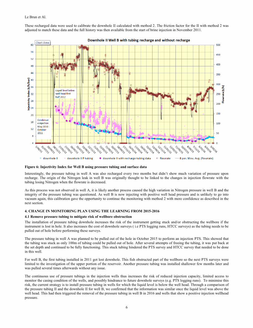
For well B, the pressure tubing was leaking Nitrogen regularly. The recharge occurred every two months and showed important

variation in pressure (+ 10 bar upon recharge). The confidence level in the pressure data from this tubing was thus not high enough to

use all the pressure data. The high variation of II using all these data is shown on Figure 6 with light pink markers. Using only the

recharged pressure data, the Injectivity evolution of the well looks more reasonable (pink diamond on Figure 6).

Le Brun et Al.

6

These recharged data were used to calibrate the downhole II calculated with method 2. The friction factor for the II with method 2 was

adjusted to match these data and the full history was then available from the start of brine injection in November 2011.

Figure 6: Injectivity Index for Well B using pressure tubing and surface data

Interestingly, the pressure tubing in well A was also recharged every two months but didn’t show much variation of pressure upon

recharge. The origin of the Nitrogen leak in well B was originally thought to be linked to the changes in injection flowrate with the

tubing losing Nitrogen when the flowrate is decreased.

As this process was not observed in well A, it is likely another process caused the high variation in Nitrogen pressure in well B and the

integrity of the pressure tubing was questioned. As well B is now injecting with positive well head pressure and is unlikely to go into

vacuum again, this calibration gave the opportunity to continue the monitoring with method 2 with more confidence as described in the

next section.

4. CHANGE IN MONITORING PLAN USING THE LEARNING FROM 2015-2016

4.1 Remove pressure tubing to mitigate risk of wellbore obstruction

The installation of pressure tubing downhole increases the risk of the instrument getting stuck and/or obstructing the wellbore if the

instrument is lost in hole. It also increases the cost of downhole surveys ( i.e PTS logging runs, HTCC surveys) as the tubing needs to be

pulled out of hole before performing these surveys.

The pressure tubing in well A was planned to be pulled out of the hole in October 2015 to perform an injection PTS. This showed that

the tubing was stuck as only 100m of tubing could be pulled out of hole. After several attempts of freeing the tubing, it was put back at

the set depth and continued to be fully functioning. This stuck tubing hindered the PTS survey and HTCC survey that needed to be done

in this well.

For well B, the first tubing installed in 2011 got lost downhole. This fish obstructed part of the wellbore so the next PTS surveys were

limited to the investigation of the upper portion of the reservoir. Another pressure tubing was installed shallower few months later and

was pulled several times afterwards without any issue.

The continuous use of pressure tubings in the injection wells thus increases the risk of reduced injection capacity, limited access to

monitor the casing condition of the wells, and possibly hindrance to future downhole surveys (e.g. PTS logging runs). To minimise this

risk, the current strategy is to install pressure tubing in wells for which the liquid level is below the well head. Through a comparison of

the pressure tubing II and the downhole II for well B, we confirmed that the information was similar once the liquid level was above the

well head. This had then triggered the removal of the pressure tubing in well B in 2016 and wells that show a positive injection wellhead

pressure.

Le Brun et Al.

7

4.2 PTS campaign to confirm reservoir processes highlighted with the II monitoring

The observed reduction in downhole II with method 2 and method 3 combined with the stable reservoir pressure identified in Well A

and the nearby monitoring wells indicated the reduction in II was likely related to a decrease in formation permeability. Confirming this

reservoir process was important as understanding the mechanism of injection decline helps define what type of solution could be

derived to reduce this decline (e.g. field management strategies).

In order to confirm the information from the pressure tubing and our hypothesis on the reservoir process, additional downhole data were

gathered. A PTS campaign was performed on well B, 2 other injection wells and on 1 monitoring well (well Z). This campaign aimed at

confirming the stable reservoir pressure, the reduction in permeability around the wellbores, and confirming that deposition was not

occurring on the casing walls.

The reservoir pressure of the monitoring well Z was confirmed constant by comparing the pressure tubing information with the PTS

results as illustrated on the Figure 7. The well Z pressure tubing is also showing signs of Nitrogen leakage (i.e scattering of the dark red

circles between 2013 and 2016), the pressure values when the tubing was recharged (large red circles) are thus used for comparison with

PTS data (blue circles).

Figure 7: Pressure data in the monitoring well Y showing agreement between the recharged values of the tubing (brigh red

circles) and the PTS data (blue circles)

Regarding the permeability of the formation, the PTS campaign in 2010 identified the deeper feedzones declining faster in injectivity

than the shallower feedzones. This concept was again observed in the 2016 PTS for 2 wells. A near wellbore damage zone around well

B was also observed using a pressure transient test, with a skin factor estimated at +2. This information indicated the decline in II

observed with the monitoring was mainly due to permeability damage near wellbore.

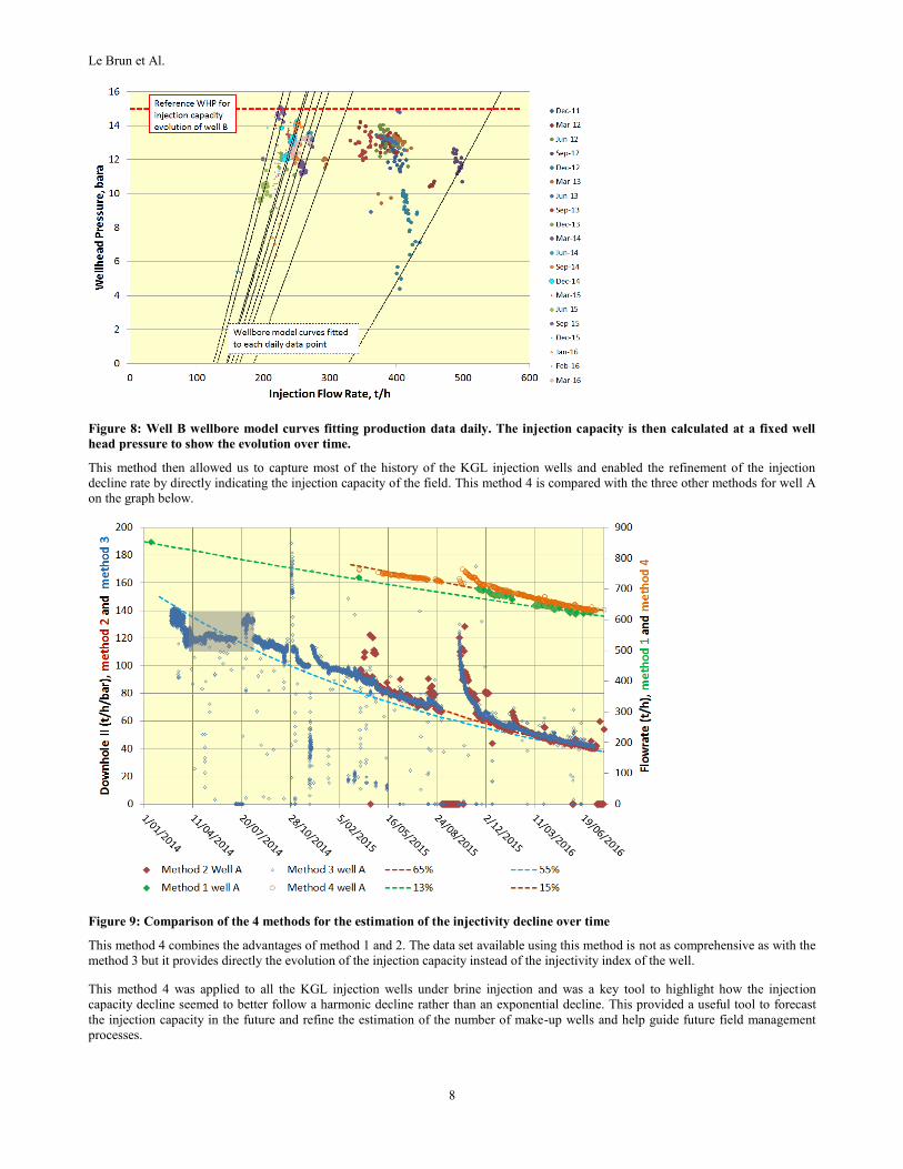
4.3 Use of wellbore modelling to transform injectivity into injection capacity

The comparison of method 2/method 3 and method 1 showed the need to translate the II decline into a mass capacity decline. Then

method 4 was designed by creating reference wellbore models for each well, with a constant reservoir pressure, and running each

wellbore model in batch mode. This batch mode changes the II in the wellbore model to fit each daily observation and then understands

the capacity along the calibrated injection curve at a constant specific WHP.

This process is illustrated on Figure 8 below with the daily injection data of well B organized by monthly series. This method is valid

for the periods when the liquid level is above the well head for each well.

Le Brun et Al.

8

Figure 8: Well B wellbore model curves fitting production data daily. The injection capacity is then calculated at a fixed well

head pressure to show the evolution over time.

This method then allowed us to capture most of the history of the KGL injection wells and enabled the refinement of the injection

decline rate by directly indicating the injection capacity of the field. This method 4 is compared with the three other methods for well A

on the graph below.

Figure 9: Comparison of the 4 methods for the estimation of the injectivity decline over time

This method 4 combines the advantages of method 1 and 2. The data set available using this method is not as comprehensive as with the

method 3 but it provides directly the evolution of the injection capacity instead of the injectivity index of the well.

This method 4 was applied to all the KGL injection wells under brine injection and was a key tool to highlight how the injection

capacity decline seemed to better follow a harmonic decline rather than an exponential decline. This provided a useful tool to forecast

the injection capacity in the future and refine the estimation of the number of make-up wells and help guide future field management

processes.

Le Brun et Al.

9

CONCLUSION

The use of three different methods to monitor the injectivity decline in two specific wells in the Kawerau geothermal field was a key

workstream in the review of the injection decline mechanism for the KGL injection wells in 2015-2016. The use of pressure tubing was

the backbone of method 3 that provided a calibration tool for method 2 and a confirmation of reservoir pressure over time.

This process gave more clarity on the rate of decline in injectivity and was a starting point to develop the method 4 that is now used to

forecast the injection capacity of the KGL injection wells. The challenges and advantages of each of these methods is summarized in the

table below using the example of well A.

Following this 2015-2016 study, the use of pressure tubing in injection wells is more targeted. The tubing is removed from the injection

wells developing positive well head pressure and expected to stay on brine injection. A pressure tubing will be installed in a newly

drilled injection well in which the liquid level is expected to be below the well head during the first months of brine injection.

This injectivity monitoring was also an essential element, along with geochemistry modeling, and field testing on the wells and plant, to

confirm the reservoir process causing injection decline. This understanding of the process causing silica deposition near well bore of the

injection wells is currently being used to derive an efficient injection strategy that will reduce the number of make-up wells needed to

optimize the plant generation.

The next step is to use the learning of this injectivity monitoring review on the Rotokawa field where several injection wells also have a

pressure tubing installed.

REFERENCES

Addison, S., Brown, K., Hirtz, P., Gallup, D., Winick, J., Siega, F., Gresham, T.: Brine Silica Management at Mighty River Power, New

Zealand, Proceedings, World Geothermal Congress, Melbourne, Australia (2015)

Askari, M., Azwar, L., Clark, J., Wong, C.: Injection management in Kawerau geothermal field, Proceedings, World Geothermal

Congress, Melbourne, Australia (2015)

Clearwater, J., Azwar, L., Barnes, M., Wallis, I., Holt.: Changes in Injection Well Capacity During Testing and Plant Start-up at

Ngatamariki, Proceedings. World Geothermal Congress, Melbourne, Australia (2015)

Grant, M.A., Bixley, P.F.: Geothermal Reservoir Engineering, 2nd Edition, Book, Academic Press (2011)

Grant, M.A, Clearwater, J., Quinao, J., Bixley, P., and Le Brun, M.: Thermal stimulation of geothermal wells: a Review of Field Data,

Proceedings, 38th Workshop on Geothermal Reservoir Engineering, Stanford University, Stanford, CA (2013).

Lim, Y.W., Grant, M.A., Brown, K., Siega, C., and Siega, F.: Acidising Case Study - Kawerau Injection Wells, Proceedings, 36th

Workshop on Geothermal Reservoir Engineering, Stanford University, Stanford, CA (2011).

Siega, C., Grant, M.A., Bixley, P., Mannington, W.: Quantifying the effect of temperature on well injectivity, Proceedings, 36th New

Zealand Geothermal Workshop, Auckland, NZ (2014)

Wong, C., Buscarlet, E., Addison., Le Brun.: Reactive transport modeling of injection fluid – Reservoir Rock interaction, Proceedings,

38th New Zealand Geothermal Workshop, Auckland, NZ (2016)

MethodsDecline rate

(% p.a)

Applied to Well A Most likelyLow

decline

High

decline

Stable

operating

WHP

WHP >

saturation

pressure

Tubing

recharged

Reservoir

pressure

Pivot point

depth

Casing Friction

factor /

roughness

Number

of data

points

Link to

injection

capacity

1 - Normalised mass flow 11% 10% 14% × × √ √√

2 - Downhole II 58% 55% 65% × × × × √√ √

3 - Tubing II 48% 45% 50% × × × (×) √√√ √

4 - Wellbore model 13% 11% 15% × × × √√ √√√

Uncertainty on

decline rateChallenges for building the monitoring data sets

Advantages for the

monitoring