Monitoring Design Guidance for the Central Valley

Irrigated Lands Regulatory Program

November 2007

i

Acknowledgements The monitoring design guidance presented below was developed in a series of meetings by members of the Irrigated Lands Regulatory Program’s Technical Issues Committee (TIC) working together with staff of the Central Valley Regional Water Quality Control Board and Dr. Brock Bernstein with the Southern California Coastal Water Research Project.

1

Introduction The following sections present design guidance for the monitoring and other studies needed to address the five basic Program questions in the Irrigated Lands Conditional Waiver Program Coalition Group Monitoring and Reporting Program (MRP Order). The various monitoring approaches described are intended to provide alternatives that allow for utilizing different approaches that are most appropriate depending on the specific question to be addressed and the degree to which the coalition has already developed the answer(s) to the questions. This guidance is intended to help organize monitoring design efforts so that the resulting designs are technically sound and cost-effective, make maximum use of existing knowledge, and balance desired consistency across programs with the flexibility needed to adapt to local circumstances. One way to envision this guidance is in terms of a performance framework, in which the outcomes or criteria for success are defined but the actual methods used to achieve the desired outcomes are flexible, though subject to performance standards. The monitoring design guidance describes approaches intended to respond to the range of conditions likely to be encountered by coalitions as they address the five Program questions that motivate the MRP Order. These alternatives should be implemented with the following basic monitoring design principles in mind: • Monitoring should be focused on decision-making; data unhelpful in making a

decision about clearly defined regulatory, management, or technical issues should not be collected. This ideally requires that the method for making the decision be clearly defined

• The level of monitoring effort should reflect the potential for water quality impact, with more monitoring allocated to situations where the potential impact (in terms both of the probability of an impact’s occurrence and its extent and magnitude) is higher and less monitoring to situations where such potential is lower or where monitoring is not likely to provide useful information

• Monitoring should be adaptive, in terms of its ability to both trigger follow-on studies as needed and make necessary mid-course corrections based on monitoring findings

In addition to following these basic principles, all monitoring and other studies implemented as part of the MRP should specifically follow accepted monitoring design practice (Figures 1 – 4) to ensure that monitoring produces the information needed to improve basic understanding, resolve uncertainties, answer the Program questions, and provide the basis for decision making. The steps in Figures 1 – 4, adapted from a National Academy of Sciences report on monitoring, are broadly applicable to a wide range of study types, from initial scoping studies to more formal, long-term trend monitoring efforts. Proposed monitoring plans for each Program question should demonstrate that they have addressed each issue in the flowcharts in Figures 1 – 4 and provide a rationale for each design decision. Such rationales may be developed at varying levels of detail, depending on the amount and kind of available information, the

2

complexity of the proposed monitoring design, and the type(s) of question(s) being addressed. The MRP Order defines the requirements for three types of monitoring (Assessment, Core, Special Projects) needed to answer the five Program questions. These monitoring types are applicable to the five Program questions as shown in Table 1. In general, Assessment monitoring is intended to describe condition and contribute to a description of long-term trends, Core monitoring focuses on describing trends, and Special Projects on targeted, site-specific studies such as source identification. A number of other monitoring efforts occur in or adjacent to Coalition areas that could provide opportunities for data and cost sharing. Coalitions are encouraged to establish working relationships with other monitoring efforts (e.g., NPDES point source, NPDES stormwater, TMDL monitoring, independent watershed groups, SWAMP) within the coalition boundaries, and whenever possible, to develop a watershed-based monitoring approach. The Central Valley Regional Water Quality Control Board (Water Board) will work directly with parties to eliminate, whenever possible, hurdles that exist between regulatory programs (e.g., permit revisions) that prohibit or delay the development of integrated watershed-based monitoring designs.

Program Questions The MRP Order identifies five key Program questions intended to structure both monitoring and management activities related to the potential impacts of agricultural discharges on surface water quality. These questions are: • QUESTION No.1: Are conditions in waters of the State that receive discharges of

wastes from irrigated lands within Coalition Group boundaries, as a result of activities within those boundaries, protective of beneficial uses?

• QUESTION No.2: What is the magnitude and extent of water quality problems in waters of the State that receive agricultural drainage or are affected by other irrigated agriculture activities within Coalition Group boundaries, as determined using monitoring information?

• QUESTION No.3: What are the contributing source(s) from irrigated agriculture to the water quality problems in waters of the State that receive agricultural drainage or are affected by other irrigated agriculture activities within Coalition Group boundaries?

• QUESTION No.4: What are the management practices that are being implemented to reduce the impacts of irrigated agriculture on waters of the State within the Coalition Group boundaries and where are they being applied?

• QUESTION No.5: Are water quality conditions in waters of the State within Coalition Group boundaries getting better or worse through implementation of management practices?

3

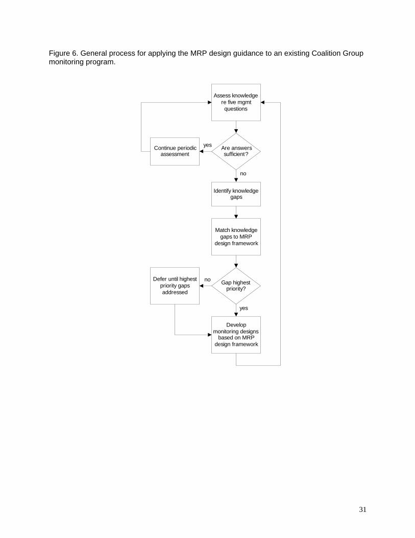
Coalitions have been conducting water quality monitoring in varying degrees in many parts of the Central Valley. Thus, important steps, such as basic assessments of condition or source identification studies, have been completed in some areas. In addition, the degree to which the five Program questions have been addressed varies substantially across the region, in part due to differing monitoring histories and in part due to the diverse nature of surface waters in different parts of the region. This is clearly documented in the zone evaluation sections of the 2007 Monitoring Data Review (Zone Reports). There is no assumption that each Coalition Group is starting with a blank slate, nor that each Coalition Group will implement the MRP Order’s monitoring guidance in a linear, stepwise fashion. Nor is it necessarily envisioned that all five Program questions will be addressed simultaneously. Instead, as Figure 5 illustrates, different Coalition Groups might enter the process at different points for different watersheds, and the MRP Order is intended to improve each Coalition Group’s ability to document linkages among the five Program questions, over some appropriate period of time. This is best accomplished through the following three steps (see also Figure 6): 1. Evaluate the Coalition Group’s ability to answer each of the five Program questions

with the information presently available, with the understanding that the ability to answer may vary from waterbody to waterbody

2. Identify critical gaps in knowledge (e.g., inability to document impacts, lack of knowledge about potential sources, absence of trend monitoring component) relevant to the Coalition Group’s specific circumstances

3. Description of how the MRP Plan is designed to fill data gaps and answer the five Program questions, including development of monitoring components suited to each Coalition Group’s circumstances, documenting how the five key Program questions will be answered.

The Zone Reports document important differences among areas of the Central Valley in terms of relative knowledge about the condition of surface waters and in design and coverage of monitoring programs. Such differences confirm that implementing the MRP Plans will most likely involve focusing on different questions, and thus emphasizing different designs, for different Coalition Groups. For example, source identification designs (Questions 3 and 4) might be the initial emphasis for one Coalition Group, but trend monitoring designs (Question 5) for another. The overall objective of the MRP is that each Coalition Group will fully address each of the five Program questions over an appropriate period of time and in a manner that makes the best use of existing information. The MRP Order is not intended as a “copy and paste” list of static monitoring requirements. Rather, its intent is to provide monitoring design guidance in sufficient detail to assure consistency in approach, but also allow for site-specific modifications and adaptations as necessary.

4

Program Question 1: Assessment Monitoring Program Question 1 is essentially an assessment question with the goal of characterizing water quality conditions and assessing whether they are protective of beneficial uses:

Are conditions in waters of the State that receive discharges of wastes from irrigated lands within Coalition Group boundaries, as a result of activities within those boundaries, protective of beneficial uses?

A subsidiary goal of assessment monitoring is to provide the foundation for developing monitoring designs to answer Program Questions 2 – 5.

Prerequisites for monitoring design Developing the details of an assessment monitoring design requires clearly defining several inputs to the design and then organizing these in a logical framework that supports effective decision making about indicators, site locations, and monitoring frequency. The logical framework should describe: 1. The basic geographic and hydrographic features of the area, particularly discharge

points and the pathways(s) of discharge flows 2. Agricultural practices and how they are distributed in space and time 3. Relevant knowledge about the transport, fates, and effects of key pollutants,

including best- and worst-case scenarios 4. Description of the beneficial uses in each water body 5. Relevant knowledge about the action of cumulative and indirect effects, and of other

sources of impact 6. Mechanisms through which agricultural practices could lead to beneficial use

impacts, given the basic features of the area (based on 1 – 5) 7. Known and potential impacts of agricultural practices on water quality (based on 1 –

5), ranked in terms of relative risk, magnitude, and severity 8. Information about sources of bias and variability, especially over different time and

space scales, that could affect the validity of a monitoring design and/or the reliability of monitoring data. This information may be qualitative or quantitative, depending on the specific requirements of the relevant monitoring design process

This information should be sufficient to describe basic patterns and processes related to impacts from agricultural drainage. The adequacy of existing information will depend on explicit decisions about: • The spatial and temporal resolution required for reliable descriptions of basic

patterns and processes • The acceptable level of uncertainty about the sources, mechanisms, locations, and

scale of potential impacts • The data analysis methods used to quantify aspects of condition related to beneficial

use

5

• The set of core indicators needed to ensure a basic level of comparability across all areas

If available information is not adequate to meet the prerequisites described above, then additional monitoring or special studies may be considered to fill these knowledge gaps. In addition, the assessment of Program Question 1 should be repeated on a periodic schedule, using a coordinated monitoring design that incorporates one or more of the approaches suggested below.

Monitoring approaches Several types of monitoring sites can be combined into one or more basic design approaches. All of these might play a role in an assessment monitoring design, depending on the extent of existing knowledge and the information in the numbered list above. More importantly, the choice of a long-term assessment design should be tightly linked to approach(es) for conducting data analyses and making judgments about the condition of receiving waters that have been jointly agreed to by the respective Coalitions and the Water Board. Types of monitoring sites include: • Long-term, usually fixed, bottom of watershed, integrator sites to assess cumulative

water quality and aggregate loads • Spatially extensive, perhaps randomly sited or rotating, stations to support

statistically valid comparisons across multiple areas or watersheds • Targeted sites based on explicit hypotheses about the times and locations where

specific types of impacts will be most visible or most severe • Fixed, site-specific stations focused on the status of high-priority locations or

habitats of concern Types of designs that use such sites include: • Cumulative effects designs in which fixed or rotating downstream sites are located

at the bottom ends of watersheds or at major confluences to document impacts of upstream sources. Such designs are based on the assumption that pollutants, and the impacts they cause, accumulate along the upstream-downstream gradient, rather than diffuse locally. While cumulative impact designs can require fewer sampling sites than the other designs described, they run the risk of not being able to capture sporadic or intermittent impacts, resolve overlapping impacts, or provide enough detail to provide an adequate starting point for source identification studies.

• Probability based designs in which stations are located randomly in order to provide the ability to draw statistically valid inferences about an area as a whole, rather than just the site itself. Such designs, for example, can permit statements about the percentage of the area that is above/below particular levels of different indicators. Such designs can allocate monitoring sites randomly throughout the entire region, or can subdivide the region into a number of strata that are relatively homogeneous. Strata can be defined on any number of grounds, depending on the

6

questions or concerns motivating the program. For example, watershed strata could be based on crop types, agricultural practices, relative amount of urbanization, general habitat type, or channel morphology, among others. Whatever the stratification scheme, the basic design principle is that samples are allocated randomly among strata, with the number of samples per stratum based on a consistent weighting factor (e.g., area of the respective strata). The level of sampling effort required in probability based designs depends, as in all designs, on the specific questions being asked, the underlying levels of variability in the data, and on the level of precision needed for decision making

• Systematic designs in which stations are located at set intervals along one or more underlying spatial or conceptual frameworks. For example, regional stations could be located on a 1-mile grid, every 1-mile along each river, creek, or stream, at every major discharge into rivers, and so on. One value of systematic designs is that they allow for more detailed mapping of indicator levels across a region. In addition, if resources permit, systematic designs can provide more thorough coverage than do probability based designs. The sampling requirements in systematic designs are typically based on the degree of spatial resolution desired

• Hypothesis-testing designs in which monitoring sites are located at times and places to test explicit expectations about where specific types of impacts will be most visible or most severe. Such designs can be more efficient than the other designs described, because they not only increase the probability of detecting impacts but also of rigorously evaluating the presumed mechanisms that lead to impacts. Hypothesis-testing designs contrast with the other four types of designs in being based directly on mechanistic assumptions about how impacts occur. Thus, they incorporate information about crop types, hydrography, drainage characteristics, pesticide application, management practices and other factors that directly or indirectly affect receiving water impacts. In addition, hypothesis-testing designs typically involve upstream, edge-of-field sampling as opposed to the downstream sampling in the cumulative effects designs. While it can be challenging to identify appropriate sites that are representative of the range of impact conditions, hypothesis-testing designs allow for the use of powerful statistical methods (e.g., ANOVA, regression) that focus on direct assessment of presumed impact mechanisms

• Rotating designs in which a different subset of stations is sampled during each sampling event, with the goal of sampling the entire set of stations over a certain period of time. Such designs have the virtue of maximizing the impact of limited monitoring resources because the entire suite of monitoring stations need not be sampled each time. However, because conditions change over time, rotating designs have a diminished ability to support valid comparisons between sets of stations sampled at different times in the rotation schedule. This can be compensated for to some extent by defining comparisons of interest during the design process and then ensuring that such stations are sampled during similar index periods or seasons. The location of stations in rotating designs can be random, systematic, or early warning depending on the kinds of questions being asked

7

These alternative design approaches are not mutually exclusive. Hybrid designs are possible, as is moving from one design to another over time depending on monitoring findings. In addition, all of these design approaches can benefit from modeling intended to estimate key parameters and processes such as transport, dispersion, and/or accumulation; chemical transformation; or bioaccumulation.

Monitoring frequency, site replacement, and site representativeness There is no set monitoring frequency that is necessarily appropriate for each type of design. In general, however, cumulative designs monitor at a regular frequency (i.e., at fixed intervals) or focus on major discharge events (i.e., those few events that transport the majority of water, sediment, or pollutant load), while probability-based designs typically monitor once or twice a year during some standard index period (i.e., a period chosen to represent overall conditions and assumed to be similar in key respects from year to year). Systematic designs monitor at regular intervals or at an index period and hypothesis testing at a frequency based on underlying impact mechanisms being evaluated, while rotating same as probability. These patterns are summarized in Table 2. One of the three monitoring design principles described in the Introduction is the need for monitoring to adapt by making mid-course adjustments based on monitoring findings. In particular, this may involve suspending monitoring at an assessment site, either periodically or permanently. Rotation among sites is inherent in the probabilistic and rotating designs described above. However, the information return from designs with fixed sites may decline over time if conditions are stable. Thus, if there are only scattered or no exceedances for a period of time (to be determined in consultation with Water Board staff) or if a source investigation has been completed that identified and eliminated the source of previous exceedances, then monitoring resources could be reallocated to another location and the site revisited several years in the future. Decisions about reallocating monitoring effort in such circumstances should include a consideration of the: • Time period of monitoring • Number of data points available • Spatial and temporal pattern of any exceedances • Magnitude of any exceedances • Type of constituent(s) involved • Rationale for concluding that future exceedances are unlikely The five-year period of the Coalition Group Conditional Waiver provides a convenient timeframe for reconsidering Coalition Group monitoring designs under the MRP Order. In addition, a Coalition Group can discuss the need for adapting its monitoring design at any time with Water Board staff. If changes are warranted, monitoring programs can be adjusted by action of the Water Board’s Executive Officer. Assessment designs will not be able to sample every watershed or discharge point. This requires that two sorts of definitions be addressed in the assessment design. First, the

8

area(s) each site is assumed to be representative of must be clearly defined. For example, a site at the bottom of a watershed could represent the upstream drainage area, while a site that samples discharges that stem predominantly from one crop type could represent other areas dominated by that crop. As another example, storm samples might be considered representative only of that condition, rather than also of low flow conditions. These definitions will be crucial to determining the scope of subsequent efforts to identify sources and implement target management practices based on the assessment monitoring information.

Program Question 2: Magnitude and Extent Monitoring Program Question 2 focuses on describing the relative severity and extent of receiving water problems identified by the assessment monitoring performed under Program Question 1. Program Question 2, as is Program Question 1, is intended to be addressed at the scale of an individual coalition. Program Question 2 is:

What is the magnitude and extent of water quality problems in waters of the State that receive agricultural drainage or are affected by other irrigated agriculture activities within Coalition Group boundaries, as determined using monitoring information?

In addition to the Program questions flowchart in Figure 5, this question corresponds to the prioritization question near the top of the flowchart in Figure 7, which focuses in more detail on subsequent source identification efforts. This information is necessary for assessing the relative severity or importance of different problems, ranking and targeting source identification efforts, and planning management actions such as source control or reduction efforts. It is important to stress that any such ranking is not meant to remove or replace regulatory requirements for the development of management plans or other actions. Rather, answers to Program Question 2 are intended to assist in developing management plan timelines, scoping source identification studies and management practice implementation, and otherwise matching the scale and timing of monitoring and management actions to the severity of water quality problems. In most cases, assessment monitoring designs to answer Program Question 1 will include only sites that are representative of specific areas and/or conditions. Thus, once a receiving water problem is found, data from these sites will most often be insufficient to characterize the full extent and magnitude of the problem and additional studies will normally be called for. This is because information about the severity of a problem is useful for prioritization before proceeding with some corrective action. Impacts that cause more extreme effects, cover large areas, or extend over long periods of time typically require more immediate attention. Impacts that cause less extreme, more localized, and or more sporadic effects can be dealt with on a longer timeline and/or with less intensive efforts. In some cases, the extent, magnitude, and/or severity of a receiving water problem will be immediately apparent from the assessment monitoring data obtained under Program

9

Question 1. In such cases, for example, high levels of toxicity in multiple test species, especially in areas of biological significance, or obvious kills of resident species in the receiving water that extend over several contiguous monitoring sites, source identification work should begin promptly. In addition, lower levels of toxicity that persist at the same sampling sites over multiple monitoring events should also be a high priority for source identification work. In other cases, broader sampling to assess spatial and temporal extent will be required, usually as special studies that, as opposed to routine monitoring, have explicit starting and ending dates. However, it may be necessary for such studies to extend over multiple years to adequately capture signals from pesticides that are only intermittently used. Thus, magnitude and extent studies focused on different types of impacts or constituents may require different timeframes depending on the characteristics of the problem being focused on. In some situations, where the problem is complex and/or covers a large area, addressing Program Question 2 will involve regional studies, perhaps initiated or organized by the Water Board, that require the cooperative efforts of several entities. It may be useful, especially during initial monitoring for magnitude and extent, to adjust data quality objectives to accommodate the rapid collection of larger amounts of data. For example, test kits and other methods can provide useful indications of the presence and relative magnitude of contamination that could help to focus further studies, even without achieving the lower levels of detection required for other types of monitoring. In addition to the spatial and temporal extent of a receiving water problem, additional studies may help to characterize the relative severity of the problem. Toxicity tests at different dilutions may better quantify the degree of toxicity (e.g., when 100% mortality is observed), while toxicity tests on different test organisms may provide greater insight into the breadth of toxic impacts. Body burden data from animals exposed to water and/or sediment from impacted sites may indicate whether and to what degree contaminants are being bioaccumulated. Similarly, laboratory bioaccumulation experiments, chemical analysis of sediment pore water, and pore water toxicity tests can furnish insight into the possible mechanisms of bioaccumulation. Finally, impacts may be judged more severe or significant if they directly affect more highly valued resources. For example, impacts on species listed as endangered or threatened under the Endangered Species Act (ESA), on highly valued recreational or commercial species, or on species with key ecological roles, are likely to be considered more important, and higher priorities, than impacts in areas or on species without these concerns. In summary, monitoring and/or data analysis to establish the extent and magnitude of receiving water impacts may include the following, with the understanding that “magnitude” includes both quantitative and qualitative estimates of severity and/or significance: • The routine monitoring sites(s) in the area of interest

10

• Estimates of the relative magnitude of toxicity or chemical exceedance, which may require additional toxicity tests at different dilutions and/or with different test organisms

• The type of pollutant(s) involved (e.g., highly toxic pesticides vs. nutrients, pollutants with numeric Basin Plan objectives vs. those without such objectives, prohibited pesticides)

• Measures of the spatial extent of actual impact in receiving waters, which may require an array of upstream / downstream samples, regularly spaced grids, or random arrays

• Measures of the temporal persistence or pattern of receiving water impact, such as over the course of a storm, between dry and wet weather, or different crop cycles, which may require sampling more intensively over either short time periods or over multiple seasons or years

• Field and/or laboratory studies to characterize the potential for bioaccumulation and the pathways by which this might occur

• Estimates of the potential risk to human or aquatic health • Documentation of whether impacts overlap or affect listed species, highly valued

recreational or commercial species, or species with key ecological roles. Such documentation may necessarily be less quantitative than that for the previous items in this list

• Whether the constituent is a legacy pollutant • Whether the problem occurs during dry and/or wet weather, since the extent of dry

weather problems may be more easily identified • Regulations and other legal mechanisms that require source identification and/or

control • Stakeholder involvement such as watershed group planning priorities This information should form the primary basis for prioritizing follow-up source identification efforts, as represented by the box near the top of the flowchart in Figure 7 (i.e., Prioritize areas). There is no standard, uniform method for integrating a variety of information such as this into a set of priority ranks. However, Table 3 presents a simple approach to developing priorities based on three data types that could be extended to additional data types. A more rigorous approach is described in Appendix 1, which presents a quantitative method for ranking toxicity testing results based on the severity (mortality), breadth (number of test species involved), and persistence (percentage of surveys with toxicity) of toxicity. The actual prioritization method used in any particular instance will depend on the nature of the problem. For example, there may well be instances in which more localized problems would be addressed first if they are likely to be more readily solved. Thus, larger regional-scale problems, such as salt, may be more appropriately dealt with by collaborative regional processes rather than by individual coalitions.

11

Program Question 3: Source Identification Monitoring This question corresponds to the portions of the flowchart in Figure 7 related to the identification of sources and the prioritization of inputs. Once monitoring or other studies demonstrate that there is a current impact to receiving waters (Program Question 1) and describe the problem’s extent and magnitude (Program Question 2), decisions about any management responses depend on information about the source(s) of the problem. Program Question 3 is:

What are the contributing source(s) from irrigated agriculture to the water quality problems in waters of the State that receive agricultural drainage or are affected by other irrigated agriculture activities within Coalition Group boundaries?

Gathering this information can be envisioned as a two-step process. The purpose of this two-step process is to prioritize more detailed source identification efforts at only those problems for which agricultural discharges are a significant contributor. The first step is an estimation of the relative importance of the agricultural contribution to the receiving water problem. Based on this estimate, source identification will proceed either as a regional collaborative effort that involves other sources (e.g., urban runoff) or as an independent effort conducted by one or more of the agricultural coalitions.

Are agricultural sources significant? It is important to clarify that defining the overall contribution of agricultural discharges is not intended in any way to diminish or replace regulatory requirements to reduce contaminant inputs to the maximum extent practicable. It is rather intended to help determine when additional, more detailed and extensive, source identification efforts should be conducted independently by a coalition or its members, with the goal of ensuring that the full burden of water quality improvement work not be shifted to the agricultural sector where action by them would not contribute significantly to solving the larger problem. The decision-making framework (Figure 1) assumes that, if agricultural discharges contribute only a very small percentage (e.g., in terms of loads of a pollutant) to the receiving water problem, then there would be no need for a coalition or its members to independently carry out substantial and broad-based source identification efforts. In such cases, regional collaborative efforts involving other types of sources should be implemented in a timely manner. A working rule of thumb would be that a coalition would not need to independently conduct source identification studies if the agricultural contribution to the problem was less than about 5 – 10%. This range is not intended as a definitive cutoff point or compliance level. It is instead intended to provide a sense of when an agricultural coalition should approach the Water Board and/or other categories of sources to propose collaborative source identification efforts. Because it is intended only as approximate guidance, this first-cut at source allocation requires only minimal resolution appropriate to a scoping study and including at least a rough estimate of the identity and magnitude of the non-agricultural contributions. For example, this first-cut

12

evaluation could include basic information about whether specific constituents are applied by agriculture or whether they are mobilized or concentrated by agricultural practices. It is thus something that should be conducted primarily with available data and completed relatively rapidly. In many situations, aggregate estimates of the non-agricultural contribution, rather than source-by-source estimates, may be adequate and may already be available from previous characterization and/or monitoring studies. While a variety of methods may be suited to deriving this first-cut estimation, they should include all readily available quantitative information, use at least simple mass-balance estimates or models, clearly state all underlying assumptions and/or algorithms, and quantify uncertainties to the greatest extent possible, especially where the agricultural contribution is near the 5 – 10% threshold. For example, if the agricultural contribution is small (i.e., less than 5% of the cumulative load), there would probably be no need to refine the estimate any further because large variability does not change the answer to the question; agricultural discharge is still a small contribution. This would be the case where a problem is due to constituents that are not used in agriculture or whose distribution is clearly unrelated to agricultural sources. In contrast, if the agricultural contribution is 10% +/- 15%, there would be a need to refine the estimate to determine whether and to what extent to proceed to the more detailed source identification work. Thus, monitoring designs for this issue might proceed through multiple iterations to develop: • Description of all potential sources of inputs to the receiving water • Rough estimates of the relative magnitude of loads from all sources • Rough estimate of the proportional contribution of agricultural discharges to total

loads It is important to emphasize that this 5 – 10% threshold is intended as a guideline only in situations where the source of a receiving water problem is not known. Where the source(s) of such problems are known, then relevant permit conditions related to source reduction would come into play. As emphasized above, this threshold is not intended to diminish or replace permit requirements to reduce contaminant inputs to the maximum extent practicable or other regulations or legal requirements. Where the agricultural contribution to a problem is small then additional focus on improving management practices may be a more rapid and cost-effective response than participation in a larger collaborative source identification study. However, where the magnitude and extent of a problem warrants it, a more broadly based collaborative source identification study may be organized by the Water Board under one or more of the relevant regulatory programs or as a Water Board-funded study if an appropriate regulatory framework is not available. Alternatively, a coalition could initiate cooperative arrangements with other coalitions, other permittees, or regional or watershed monitoring efforts.

13

What are the sources from agriculture? Only if agricultural discharges are found to contribute significantly (i.e., more than 5 – 10% of loads) to receiving water problems would a coalition or its members be required to take the lead on conducting further source identification studies, at greater resolution, of agriculture’s contribution. Such studies would be intended to provide more detailed information about the nature, location, and quantity of inputs to the higher-priority receiving waters identified in Program Question 2. This information can help refine receiving water monitoring, improve fundamental understanding of agricultural discharge contamination processes, and help guide management actions intended to reduce sources and their attendant impacts. It can also help focus trend monitoring under Program Question 5 on those parameters that are potentially most responsive to agricultural source reduction efforts. In the context of Program Question 3, “sources” can refer to two types of sources. The first is identification of the specific chemical(s) responsible for observed impacts, while the second is identification of the specific locations or agricultural cultural practices responsible for releasing, mobilizing, or concentrating such chemicals. Figure 7 (a and b) provides a general framework for source identification efforts. It places these in the larger context of the prioritization discussed under Program Question 2 and is integrated with the implementation of management practices. There are several instances in Figure 7 that call for “Stop and consider with Water Board staff”. These refer to situations where there is no readily apparent solution to a problem and/or where additional efforts would be much less cost effective. The intention of this step is that Water Board staff and the Coalition would collaborate to review all available information and develop a strategy for moving forward. The identification of specific pollutants responsible for impacts may involve data mining, statistical, biological, and/or chemical methods, such as: • Investigation of available data from pesticide use reports, flow and discharge

patterns, patterns of crop types, and specific agricultural cultural practices, combined with chemical concentration data, to pinpoint the most likely cause(s) of impact

• Statistical analysis of the strength of correlations between the patterns of individual chemicals and biological endpoints (e.g., toxicity, benthic community condition)

• Gradient analysis that uses samples taken at various distances from an impact to examine patterns in chemical concentrations and biological responses. The concentrations of presumed causative agents should decrease as biological effects decrease

• Toxicity Identification Evaluation (TIE), a toxicological method for determining the cause of impairments. Water or sediment samples are manipulated chemically or physically to remove classes of chemicals or render them biologically unavailable. Following the manipulations, biological tests are performed to determine if toxicity has been removed or, for some sediment TIEs, enhanced. In general, TIEs are most effective where strong toxicity signals have been observed

• Bioavailability studies to determine if chemical contaminants are present but not biologically available to cause toxicity or other biological effects. For sediments,

14

chemical and toxicological measurements of pore water can determine the availability of sediment contaminants. Metal compounds may be naturally bound up in the sediment and rendered unavailable by the presence of sulfides. Measurement of acid volatile sulfides and simultaneously extracted metals analysis can be conducted to determine if sufficient sulfides are present to bind the observed metals. Similarly, organic compounds can be tightly bound to sediments. Solid phase microextraction (SPME) or laboratory desorption experiments can be used to identify which organics are available to animals

Source tracking to identify the likely location(s) and/or activities that identified contaminants stem from typically follows either a systematic or branching design template. In the systematic design template, all inputs, or a representative sample of all inputs, are sampled and quantified or ranked in terms of their relative contribution. In the branching design template, a contamination signal is followed upstream, with a decision being made at each branch point about which branch to continue following upstream, based on the strength of the signal in each tributary input. However, there are many aspects of agricultural practices and discharges that make it impractical to always apply these standard approaches to source identification. For example, flows can be highly managed and do not always follow a typical upstream – downstream pattern. Irrigation water can be held on fields, return flows can be pumped upstream to combine with source water, and water can be transferred from one field to another. In addition, the episodic nature of many pesticide applications means that a chemical signal may not persist long enough for upstream source tracking to be effective. In some instances, where a Coalition knows when a particular chemical will be applied in a specific area, monitoring can be conducted to bracket the application to confirm whether suspected activities are in fact the source of water quality impacts. There are several categories of sources likely to be encountered, each of which requires a somewhat different approach to source identification. The timeframe for each source identification study should make realistic allowance for the lag times that may be involved in acquiring certain kinds of information. For example, pesticide use reports are not always immediately available and it may require multiple seasons or years to adequately track sources of pollutants that are only applied or mobilized sporadically or at long time intervals. The following categories represent the major types of sources, but others do exist and the list is not intended to be exhaustive.

Crop-specific pesticides Examples of constituents in this category include chlorpyrifos, which is used for dormant spraying on almond and prune orchards from early January to mid-February and on alfalfa in from March through the summer. Appropriate steps for this category of inputs include: • Contact the agricultural commissioner to request pesticide use reports for a specific

crop(s), period, and/or region. There may or may not be a record of use for the

15

pesticide being investigated. It is also important to recognize that the use reports are only a first step, are not all inclusive, and do not account for discharge patterns that have a large effect on the potential for downstream impact

• Contact growers who grow the crop or use the pesticide to verify use patterns and cultural practices and to discuss the problem and ways to address it. For example, most of the chlorpyrifos use is on a couple of specific crops within a well-defined time period, e.g., dormant spray and alfalfa

• Map use patterns within different time windows to help establish a causal relationship with downstream monitoring data

• Verify that application practices comply with accepted or required management practices

• Determine the discharge pattern(s) for the period(s) of interest. Note that discharge can change daily and that discharge data may not be available for all locations, with the result that it can be hard to pin sources down to individual growers

• Surveys may be needed to help interpret the implications of the discharge patterns • Identify who has used the constituent (if possible) and contact the specific growers.

However, it may only be possible to identify users/sources to categorical levels

Broadly distributed, non-pesticide, particle-bound constituents Examples of constituents in this category include lead, PAHs, and phthalates. Appropriate steps for this category of inputs include: • Determine whether the constituent is a high priority constituent (see above) • Use a desktop audit (i.e., a rough calculation using readily available data), combined

with toxicity testing (see bullet below) to determine which beneficial uses are being impacted. Prioritize attention on where beneficial uses are being impacted

• Test the assumption that the majority of the constituent is particle bound, for example, with analyses of total and dissolved fractions. However, such information should be interpreted with care because partitioning between bound and dissolved phases can be complicated, with pollutants moving back and forth from bound to dissolved phases

• If the majority of the constituent is in fact in the particulate phase, sediment toxicity tests, combined possibly with sediment TIEs, could help partition the sediment-related toxicity into higher- and lower-priority components. These results could then help to identify agricultural constituents as either lower- or higher-priority inputs

• Determine whether the sediment-bound constituent is entering the system and moving downstream through the system or is simply being re-suspended by high flows from sediments already in the system. This may involve assessing the potential importance of in-place bed sediments in contrast to sediments imported, mobilized, and/or transported by agricultural practices

• If the constituent is entering the system, determine the entry point(s). Isotope studies can assist with such tracking; however, they are costly

• Determine if the constituent stems from legacy applications. If so, there should be an “early out” in the process, unless erosion control practices useful for other constituents would also be useful for the constituent

16

• Determine if the constituent can be added to the soil as a soil amendment or through a fertilizer

Legacy pesticides Examples of constituents in this category include DDT/DDE, dieldrin, and atraton. Appropriate steps for this category of inputs include: • Postulate that it is not currently being applied, based on evidence of sales and use,

patterns of distribution in the environment (e.g., broadly distributed with no highly localized sources), and mass balance modeling to estimate the amount remaining in the environment

• If the constituent is most commonly associated with sediments, improve understanding of how the constituent is mobilized and moves through the system, e.g., whether it is moving from fields to channels and how this happens. For example, flooding lands to drive salt further down in the soil brings in water with sediment loads that include DDT/DDE that remains on the fields after they dry out

• Conduct simple mass balance modeling, as has been done for mercury in the San Francisco Bay area, to set some rough boundary conditions on the size of the problem and the potential for addressing it

• Sediment control may be the best option to address this parameter and, if so, would provide an opportunity to deal at the same time with other sediment-related issues. Thus, source identification studies should include tracking of sediment sources, flows, and sinks, followed by an evaluation of whether sediment control practices will actually reduce downstream levels of legacy pesticides. This will involve looking at the entire drainage system, not just at the scale of individual fields

Given the regional nature of legacy pesticide contamination, and the assumption they are no longer being applied, it may be more appropriate that the Water Board lead efforts to characterize the distribution, concentrations, and sources of legacy pesticides.

Valley-wide constituents from natural sources Examples of constituents in this category include salinity, boron, and pathogens. Appropriate steps for this category of inputs include: • Evaluate existing information on sources and distribution • Determine if constituent is being used as a soil amendment or fertilizer • Estimate incremental change due to agriculture with a straightforward comparison of

input vs. output levels • Evaluate the priority level In general, such constituents will be addressed with coordinated regional programs (e.g., Salinity Workgroup) led by the Water Board and other interested agencies.

Secondary or cumulative effects Indicators in this category are not directly discharged by agriculture but instead are indirect or cumulative effects of agricultural activities. Examples of constituents in this

17

category include dissolved oxygen and pH. Appropriate steps for this category of indicators include: • Document spatial and/or temporal patterns that may affect the measurement of

magnitude, extent, and trends • Review monitoring data for information on causal inputs (e.g., nutrients) • Develop causal model that is more relevant than the usual upstream – downstream

source identification model • Identify precursors or causal inputs and determine if these should be measured • Develop “source” identification measurement plan based on the above The wide variety of specific situations likely to be encountered makes it infeasible to recommend a standard study design for Program Question 3. However, in general, monitoring and/or data analysis to estimate the potential agricultural contribution to a receiving water problem could include: • Visual reconnaissance and observation • Land use modeling • Mass balance modeling • Flow and discharge modeling to relate upstream and downstream patterns • Calculations of estimated toxicity of chemical constituents to assess whether

observed levels are high enough to be likely contributors to toxicity • TIEs to determine whether toxicity is due to the class of constituents of concern

(e.g., metals vs. pyrethroids) • The use of unique and/or conservative tracers • Evaluation of existing data, particularly comparisons of contrasting times and/or

places

Program Question 4: Management Practices Monitoring This question corresponds to the portions of the flowchart in Figure 7 related to the identification and application of management practices. Program Question 4 is essentially an inventory question that focuses on gathering and organizing information about current management practices. It reads:

What are the management practices that are being implemented to reduce the impacts of irrigated agriculture on waters of the State within the Coalition Group boundaries and where are they being applied?

Management practices fall into three levels of activity: • Level I: Outreach and education by the Coalition intended to foster changes in Level

II and Level III Management practices • Level II: Evaluating and modifying cultural practices such as pesticide application

and storage

18

• Level III: Constructing structural features such as drainage modifications and sediment retention basins

Some cultural practices and structural features undertaken for other reasons may have the indirect effect of improving water quality. Such potentially dual-purpose activities should be a particular focus of monitoring for Program Question 4. It is important to note that these three Levels of activity will not necessarily be implemented in sequence. For example, outreach and education are often conducted in parallel with evaluating and modifying cultural practices. As another example, structural management practices may not be relevant for certain water-borne constituents; on the other hand, it may be useful to implement structural management practices before sources are fully identified if they will provide other benefits, such as improving water use efficiency. Any management practices applied should meet the following criteria: • The management practice should address the problem • Management practices should be based on the body of knowledge of what we know

about what is already being done to address this problem, with new efforts incremental to, rather than duplicative of, existing efforts

• Management practice options should start with the less expensive, easiest methods to implement and progress to the more expensive and complicated methods

• Cost and efficiency should be compared with the urgency and severity of the issue • Apply the most appropriate criteria for implementing management practices and

include efforts to improve information about sources as needed Inventories of management practices will greatly assist in applying these criteria and evaluating management practice performance, though the degree of detail needed to adequately apply these criteria will differ from place to place and time to time. However, developing an inventory of management practices is complicated by the fact that there is no central database of such management practices (nor has there been a regionwide survey), there is great spatial and temporal heterogeneity in the kinds of practices used, and the coalitions are not necessarily informed about the specific practices farmers use on a field-by-field basis. Thus, while there is ongoing outreach and education, there is not yet a well-developed feedback mechanism about what practices are actually implemented. Coalitions should both track their efforts at improving management practicesby their members and conduct periodic surveys to track the degree to which management practices are being implemented. This information should be organized in such a way that it can effectively support source identification and other problem-solving efforts, as well as oversight to help ensure that management practices continue to be implemented as intended. At a minimum, this would require simple databases at the Coalition level. Ideally, such databases would be formatted similarly so that data from multiple Coalitions could be readily combined for larger, regional assessments.

19

Program Question 5: Trend Monitoring This question corresponds to the portions of the flowchart in Figure 7 related to tracking whether targets are being met. Program Question 5 is primarily a trends question that reads:

Are water quality conditions in waters of the State within Coalition Group boundaries getting better or worse through implementation of management practices?

While this is a key monitoring element, the locations of stations, the monitoring frequency, and the relative emphasis on specific indicators may depend on information developed in answer to other questions related to where problems exist (Program Question 1), the extent and magnitude of such problems (Program Question 2), the nature and number of sources (Program Question 3), and expectations for how management practices may improve conditions (Program Question 4). As with the monitoring for the other Program Questions, there are a number of alternative approaches possible for trend monitoring. In general, they fall somewhere between the two ends of the spectrum defined by: • Traditional fixed site designs in which permanent indicator or trend sites are placed

either at representative locations, where problems have been seen in the past, where key resources are at risk, or where changes are expected to be most readily detected. These fixed sites may be at upstream or downstream locations, depending on the target indicators and the nature and size of the change, or signal, expected

• Probabilistic designs, in which trends in overall condition are based on aggregated data from randomized or rotating monitoring sites. These designs can track trends in, for example, the percentage of an area that is above or below critical thresholds for different indicators. They can also track trends in estimates of average condition or the variability around mean or median values

Irrespective of the design approach used, key issues for all trend monitoring include decisions about: • The expected change in conditions to be detected due to improved management

practices • The effect of other sources of change, such as changes in land use • Indicator selection • Monitoring frequency and duration • Data analysis method(s) used to describe trend For each of these issues, a variety of data inspection, analysis, and/or modeling tools may be useful, as described in the following paragraphs. Trend monitoring designs should be based on a clear statement about what sorts of changes are expected, where they are most likely to be detected, what their magnitude is likely to be, and over what time frame they are expected to occur. Such a statement

20

will define the “signal” trend monitoring is intended to detect. This can be based on conceptual or numerical modeling, past monitoring data, and/or information from analogous or contrasting situations and provides the basis for selecting indicators, determining monitoring frequency and duration, and choosing data analysis methods. Indicators should focus on targets that are specific to each receiving water problem and/or management practice. These can include water quality parameters, levels of effort, or degree of use of particular practices. While indicators related to management practice implementation can be useful interim measures of progress, long-term trend monitoring should ultimately focus on measures of water quality and/or related beneficial uses. Determining the frequency and duration of trend monitoring is complicated by the often extreme spatial and temporal variability in overall condition as well as in specific indicators of water quality and beneficial use. While it is often assumed that trend monitoring programs will continue indefinitely, it is also important to estimate the length of time it will likely require to detect the expected change in condition. In addition, substantial improvements in overall efficiency can be achieved from optimizing the relative allocation of sampling effort to within-year vs. between-year sampling. Figure 8 illustrates results of an example statistical power analysis of a trend monitoring design. These results show that the ability of a trend monitoring program to detect a given amount of change can vary markedly, depending on how the inherent variance differs among sites and times. In the top figure, the inherent variability is so great that no amount of sampling effort would ever be likely to detect even large changes in indicator values. Such statistical power analyses can help in determining, ahead of time, how to distribute sampling effort and whether any particular trend monitoring design is likely to be able to detect a meaningful amount of change in a reasonable amount of time. The choice of data analysis method(s) has an important effect on the ability to determine whether conditions are getting better or worse over time. Such analyses can be hampered by short time series of data, inherently high variability, and poor understanding of the processes that create this high variability. There are, however, useful data visualization and regression techniques, short of formal time series analysis, that can often help reveal temporal patterns and trends in data, even when they are extremely noisy. The four examples illustrated in Figures 9 – 12 range from relatively simple to more sophisticated approaches. Figure 9 shows how data smoothing can highlight a seasonal pattern in noisy bacterial data and Figure 10 illustrates how plotting deviations from the long-term mean, as opposed to raw or even smoothed data, highlights underlying trends in the data. Figure 11 demonstrates how accounting statistically for an underlying cyclical signal, and partitioning the trend analysis into different conditions, permits the detection of a trend that exists in one condition but not the other. Finally, Figure 12 shows how tracking trends in the binary probability of an exceedance provides a clear picture of trends in condition that may not always be available when analyzing the indicator data themselves.

21

22

Table 1. Relationship between the three types of monitoring defined in the MRP Order and the five Program questions presented in the MRP Order and discussed in this guidance document. 1: Condition /

status

2: Magnitude & extent

3: Sources

4: Management practices

5: Trends

Assessment X X Core X Special Projects

X X X X

Basic Information

X

23

Table 2. Monitoring frequencies typical of the alternative potential assessment monitoring design approaches to address Program Question 1. “Regular” refers to a fixed frequency, “Index period” to a period chosen to represent overall conditions and assumed to be similar in key respects from year to year, “Discharge events” to those few events that transport the majority of water, sediment, or pollutant load, and “Impact mechanisms” to specific events or processes hypothesized to create water quality impacts.

Monitoring Frequency or Period

Design approach

Regular Index period Discharge events

Impact mechanisms

Cumulative effects X X Probability-based X Systematic X X Hypothesis-testing X X Rotating X X

24

Table 3. An example source identification prioritization, based on three commonly measured aquatic indicators. “Yes” and “No” refer to whether or not data from each component have exceeded some threshold of concern. In this illustrative example, toxicity is weighted more highly than dissolved oxygen, as seen in the “Low” priority for #5 (where dissolved oxygen is the only problem) compared with the “Medium” priority for #8 (where aquatic toxicity is the only problem). Such weighting schemes can be adjusted based on how the site-specific importance of different impacts or constituents. This template is somewhat simplistic (e.g., it does not include extent and magnitude of the problem) but outlines the sort of systematic approach needed for prioritization. An analogous approach could be used for sediment-related monitoring data.

Indicator

Yes N o Source ID Priority

1. Aquatic chemistry X Aquatic toxicity X Dissolved oxygen X High

2. Aquatic chemistry X Aquatic toxicity X Dissolved oxygen X Low

3. Aquatic chemistry X Aquatic toxicity X Dissolved oxygen X High

4. Aquatic chemistry X Aquatic toxicity X Dissolved oxygen X Low

5. Aquatic chemistry X Aquatic toxicity X Dissolved oxygen X Low

6. Aquatic chemistry X Aquatic toxicity X Dissolved oxygen X Medium

7. Aquatic chemistry X Aquatic toxicity X Dissolved oxygen X Medium

8. Aquatic chemistry X Aquatic toxicity X Dissolved oxygen X Medium

25

Figure 1. The main elements of the monitoring design process (adapted from Managing Troubled Waters. 1990. National Research Council). Steps 1 – 3 are detailed further in Figures 2 – 4.

Step 1: define expectations and goals

Step 2: define study strategy

Step 3: develop measurement strategy

Can effects be detected?

Step 4: implement study

Step 5: produce information

Is information adequate?

Step 6: disseminate information

Step 7: make decisions

Reframe questions

Rethink study approaches

Refine goals

no

yes

no

yes

26

27

Figure 2. Defining expectations and goals for the monitoring design (adapted from Managing Troubled Waters. 1990. National Research Council).

Identify management / scientific concerns and

expectations

Identify relevant technical information

Focus scientific understanding

Establish objectives and fit with MRP management

questions

28

Figure 3. Defining the monitoring study strategy (adapted from Managing Troubled Waters. 1990. National Research Council).

Identify key processes

Develop conceptual model

Appropriate processes selected ?

Determine appropriate boundaries

Are boundaries adequate?

Estimate effects / signal

Are estimates reasonable?

Develop specific , measurable questions

Modify selection

Adjust boundaries

Refine model

no

yes

no

yes

no

yes

29

Figure 4. Developing the measurement design (adapted from Managing Troubled Waters. 1990. National Research Council).

Develop specific , measurable questions

Identify meaningful levels of change / effect

Select what to measure

Develop measurement design

Specify statistical model (s)

Can effects / signal be seen?

Define data quality objectives

Develop measurement design

Is design adequate?

Implement design

Quantify / estimate variability

Identify logistical constraints

Conduct power tests / optimization

Reframe questions

Refine technical design

no

yes

no

yes

30

Figure 5. Overview of the functional relationships among the five Program questions. The answer to each question provides the basis for developing the monitoring design to answer the next. Specific monitoring programs may have addressed questions in parallel or out of sequence, depending on available knowledge and specific information needs. Thus, the process may be entered at any point, depending on the degree of current knowledge.

Determine mechanisms

causing receiving water problems

2. Determine extent and

magnitude of receiving water

problems

1. Assess conditions in

receiving waters

Are conditions protective of

beneficial uses?

Continue periodic assessment

Causal mechanisms identified?

Conduct special studies

yes

no

no

Extent / magnitude significant?

Continue periodic assessment

3. Determine relative agricultural

contribution

yesno

yes

Ag contribution significant?

no

3. Determine sources of agricultural contribution

Sources identified?

Conduct special studies

no

4. Implement / identify

management actions

yes

5. Assess trends in conditions

yes

Assign reduced priority

31

Figure 6. General process for applying the MRP design guidance to an existing Coalition Group monitoring program.

Assess knowledge re five mgmt questions

Are answers sufficient?

Continue periodic assessment

Identify knowledge gaps

Match knowledge gaps to MRP

design framework

Develop monitoring designs

based on MRP design framework

yes

no

Gap highest priority?

Defer until highest priority gaps addressed

yes

no

32

Figure 7a. Overview of monitoring and evaluation steps focused primarily on source identification efforts. See Figure 7b for additional detail related to implementing management practices.

Potential ag sources?

Apply BMPs

yes

no

Ag sources?

Input high priority?

yes

no

Reallocate source ID efforts to next highest priority

input

yes

Weight of evidence impact

ranking

Confirm not ag sources

yes

no

BMPs possible?

Stop and reconsider w/Board staff

no

Other high priority inputs?

yes

Stop and reconsider w/Board staff

no

Question 1: Assessment

Question 2: Magnitude & extent

Question 3: Sources

Question 4: Management practices

Question 5: Trends

Ag sources significant?

Collaborative source ID efforts

yes

Source ID studies

no

yes

Prioritize areas

See detail in next figure

33

Figure 7b. Detail of monitoring and evaluation process related to implementing management practices.

Apply BPs Targets met?

no

yes

More intensive source ID

Targets met?

Apply more intensive BMPs

yesYet more intensive source ID

no

Apply yet more intensive BMPs

Targets met?Stop and

reconsider w/Board staff

no

More intensive BMPs

possible?

Stop and reconsider w/Board staff

More intensive BMPs

possible?

Stop and reconsider w/Board staff

no

no

Reallocate source ID efforts to next highest priority

input

yes

yes

From previous figure

Back to previous figure

34

Figure 8. Example statistical power analysis results for a trend monitoring design that includes multiple samples per year over a number of years. The two plots represent results using sample data from two different areas with different inter- and intra-annual variance. Each curve represents a different level of within-year sampling effort (i.e., 5, 10, 20, 40 samples per year). The y-axis represents the amount of overall change in the indicator that can be detected at various combinations of sampling effort. The x-axis represents the number of years monitoring could continue. These figures can be used to estimate the ability of any combination of sampling effort to detect a specific amount of change in the indicator value. For example, the top figure suggests that a 50% change in indicator levels could never be detected even with extremely high levels of sampling effort. In contrast, the lower figure shows that a 50% change in indicator levels could probably be detected in 10 years with 40 samples per year or in about 20 years with 20 samples per year.

35

Figure 9. Example of the effect of smoothing on the ability to detect an underlying pattern in noisy data. (Example from the Wolfram Research website, www.wolfram.com)

36

Figure 10. Deviations from the long-term mean of temperature in the California Current system. (From a report of the CalCOFI program)

37

Figure 11. Linear regression of a constituent’s concentrations with data separated into two different conditions and the cyclical effect of a factor such as rainfall statistically accounted for.

38

Figure 12. Example logistic regression of the probability that a constituent’s concentrations will exceed a regulatory standard, with data separated into two different conditions and with the cyclical effect of a factor such as rainfall statistically accounted for. For the logistic regression, all raw data are converted into either a “1” for data exceeding the standard, or a “0” for data not exceeding the standard. In this example, the probability of exceeding the standard is trending in different directions in each condition.