monitoring an ecosystem at risk: what is the degree of ... · monitoring an ecosystem at risk: what...

Monitoring an ecosystem at risk: What is the degreeof grassland fragmentation in the Canadian Prairies?

Laura Roch & Jochen A. G. Jaeger

Received: 18 June 2013 /Accepted: 19 November 2013# Springer Science+Business Media Dordrecht 2014

Abstract Increasing fragmentation of grassland habi-tats by human activities is a major threat to biodiversityand landscape quality. Monitoring their degree of frag-mentation has been identified as an urgent need. Thisstudy quantifies for the first time the current degree ofgrassland fragmentation in the Canadian Prairies usingfour fragmentation geometries (FGs) of increasing spec-ificity (i.e. more restrictive grassland classification) andfive types of reporting units (7 ecoregions, 50 censusdivisions, 1,166 municipalities, 17 sub-basins, and 108watersheds). We evaluated the suitability of 11 datasetsbased on 8 suitability criteria and applied the effectivemesh size (meff) method to quantify fragmentation. Werecommend the combination of the Crop InventoryMapping of the Prairies and the CanVec datasets as themost suitable for monitoring grassland fragmentation.The gra ss l and area remain ing amounts to87,570.45 km2 in FG4 (strict grassland definition) and183,242.042 km2 in FG1 (broad grassland definition),out of 461,503.97 km2 (entire Prairie Ecozone area).The very low values of meff of 14.23 km2 in FG4 and25.44 km2 in FG1 indicate an extremely high level ofgrassland fragmentation. The meff method is supported

in this study as highly suitable and recommended forlong-term monitoring of grasslands in the CanadianPrairies; it can help set measurable targets and/or limitsfor regions to guide management efforts and as a tool forperformance review of protection efforts, for increasingawareness, and for guiding efforts tominimize grasslandfragmentation. This approach can also be applied inother parts of the world and to other ecosystems.

Keywords Effectivemesh size . Ecological indicators .

Grassland conservation . Landscape fragmentation .

Fragmentation per se . Protected areas . Prairie ecozone .

Roads . Urban sprawl

Abbreviations used

CBI City Biodiversity IndexFG Fragmentation geometryCESI Canadian Environmental Sustainability

IndicatorsFSDS Federal Sustainable Development

Strategymeff Effective mesh sizeseff Effective mesh densityAAFC Agriculture and Agri-Food CanadaSpATS Spatial and Temporal Variation in

Nesting Success of Prairie Ducks StudyCUTprocedure

Cutting-out procedure

CBCprocedure

Cross-boundary connections procedure

CD Census divisionWS Watershed

Environ Monit AssessDOI 10.1007/s10661-013-3557-9

Electronic supplementary material The online version of thisarticle (doi:10.1007/s10661-013-3557-9) contains supplementarymaterial, which is available to authorized users.

L. Roch : J. A. G. Jaeger (*)Department of Geography, Planning and Environment,Concordia University Montreal,1455 De Maisonneuve Blvd. West, Suite H1255, Montreal,QC H3G 1M8, Canadae-mail: [email protected]

L. Roche-mail: [email protected]

http://dx.doi.org/10.1007/s10661-013-3557-9

CARTS Conservation Areas Reporting andTracking System

CCEA Canadian Council on Ecological AreasRAN Representative Areas NetworkESM Electronic supplementary material

Urgent need formonitoring grassland fragmentation

Increasing threats to grassland habitats

Native grasslands have one of the richest biologicaldiversity of all the Earth’s ecosystems, includingmany species at risk (White et al. 2000; Henwood2010; Federal and Provincial and Territorial Govern-ments of Canada 2010; Samson and Knopf 1994).The shrinkage and increased isolation of remnantgrassland habitat patches lead to reductions in spe-cies richness and biodiversity, the disruption of pos-sibilities of movement, e.g. dispersal and (re-)colo-nization, the disruption of metapopulation dynamics,and a greater vulnerability and risk of extinction.Native grasslands support many important ecosys-tem services. They “provide soils and water conser-vation, nutrient recycling, pollination, habitat forlivestock grazing, genetic material for crops, recrea-tion, climate regulation and storage for about 34 %of the terrestrial global carbon stock” (Federal andProvincial and Territorial Governments of Canada2010, p. 15) and represent a major carbon sink(White et al. 2000; Henwood 2010), superior to thatof forests (Samson and Knopf 1994). When nativegrasslands are converted to other land use types,carbon is released contributing significantly togreenhouse gas emissions (White et al. 2000;Henwood 2010). Grasslands are an important sourceof food and genetic material, which is used foraugmenting crops and pharmaceuticals (White et al.2000). They are also used for recreational activitiessuch as hunting and tourism, and have significantaesthetic and spiritual properties (White et al. 2000).

Even though temperate grasslands constitute oneof the most endangered ecosystem types on Earthand have the highest risk of biome-wide biodiversityloss, they are one of the least protected biomes; withonly 4 % under protection (Henwood 2010; Federaland Provincial and Territorial Governments of Cana-da 2010; White et al. 2000). The Prairies of North

America have declined by 79 % since the early1800s (White et al. 2000). By 2003, over 97 % oftall-grass prairie, 71 % of mixed prairie, and 48 %of short-grass prairie had been lost in North America(Federal, Provincial and Territorial Governments ofCanada 2010); making grasslands the most endan-gered ecosystem in North America (CEC and TNC2005). Few grassland landscapes, that are sufficientin size to properly sustain biodiversity and ecologicalprocesses which are native to the landscape, remain(Samson et al. 2004); therefore, the need is great topreserve the few grasslands that are left. However,the estimates of the amount of grassland lost varyconsiderably between different sources as differentmethods, data sources, and definitions of grasslandtypes (Table 1) can influence such estimates. Thesevariations can also affect the estimates of the degreeof grassland fragmentation.

Increasing fragmentation due to human activitiesis a major threat to the conservation value of grass-lands, but their degree of fragmentation and rate ofchange are currently not known. The focus of thisstudy is on the grasslands in the three Prairie prov-inces (Manitoba, Saskatchewan, and Alberta), whichmake up the Prairie Ecozone of Canada. The North-ern Great Plains cover 5 % of Canada’s land area,taking up 16 % of the area of the three Prairieprovinces (Gauthier and Wiken 2003) and have“been identified as a global priority for conservation”(Henwood 2010, p. 129). Of the portion located inCanada (Prairie Ecozone), approximately 3.5 % areunder some form of conservation (Gauthier andWiken 2003).

Canada has lost 44 % of grassland species popula-tions since the 1970s (Federal and Provincial and Terri-torial Governments of Canada 2010). Edge effects fromfragmented habitat patches play an important role to thisdecline, as grassland birds avoid nesting close to theseedges (Merola-Zwartjes 2004; A1 in Electronic supple-mentary material (ESM)). The majority of the decline innative grasslands happened before the 1930s due toconversion to agricultural land (Riley et al. 2007;Gauthier and Wiken 2003). However, further alterationand degradation is still continuing, with small patchesbeing affected the most (Federal and Provincial andTerritorial Governments of Canada 2010; Samson andKnopf 1996). As a consequence, grasslands are underserious threat of further degradation and fragmentation(Table 2).

Environ Monit Assess

Monitoring is an important prerequisite for grass-land conservation (Gauthier and Wiken 2003). It isdifficult to allocate resources unless we know wherewe stand in terms of past and ongoing trends in grass-land fragmentation. Numerical data will be more useful

and provide greater accuracy than qualitative informa-tion and anecdotal observations when assessing long-term trends, when identifying areas of rapid change orhigh risk of degradation, or evaluating whether conser-vation activities are having their desired effects.

Table 1 Commonly used grassland terms and definitions in the literature

Term used Definition Source

Grasslands “…as terrestrial ecosystems dominated by herbaceous and shrubvegetation and maintained by fire, grazing, drought and/orfreezing temperatures. This definition includes vegetation coverswith an abundance of non-woody plants and thus lumps togethersome savannas, woodlands, shrublands, and tundra, as well asmore conventional grasslands”.

White et al. (2000, p. 1)

Grasslands “Less than 10% tree cover”. White et al. (2000, p. 11)

Grasslands “Grasslands generally include land that is in perennial grasses andherbaceous species for grazing or other uses including native range,seeded tame pasture, abandoned farm areas and other non-cultivateduses (e.g. ditches, riparian areas etc.). Grasslands represent anenvironment historically or currently dominated by graminoids,occurring primarily over light to dark brown chernozemic soils,under semi-arid to arid conditions with dry, warm summers”.

Gauthier and Wiken (2003, p. 362)

Grasslands “Grasslands are open ecosystems dominated by herbaceous(non-woody) vegetation”.

Federal and Provincial and TerritorialGovernments of Canada (2010, p. 15)

Native grass “Predominantly native grasses and other herbaceous vegetation mayinclude some shrubland cover. Land used for range or nativeunimproved pasture may appear in this class. Comments: Alpinemeadows fall into this class”.

Centre for Topographic Information andEarth Sciences Sector and NaturalResources Canada (2009, p. 4–5)

Native grassland “Areas vegetated with various mixtures of native grasses, forbs, andshort (<2 m tall) woody plants. Native grasslands have usuallynever been broken and are often found in large contiguous blocks,but small remnant native grasslands may remain. May containsome invasive species”.

IWWR, DUC (2011)

Planted grassland “Areas planted to introduced grasses to provide pasture. Use thiscoding when the grasses show evidence of being mechanicallyseeded (e.g. grasses are in rows, limited species diversity reflectsoriginal seed mix)”.

IWWR, DUC (2011)

Other grassland “Areas vegetated with various mixtures of introduced and nativegrasses, forbs, and short (<2 m tall) woody plants. Usuallyfound in smaller blocks but previously ploughed areas that havereverted (not planted) to introduced species are considered OtherGrassland. Use for most wetland margins and all rights-of-wayand fenceline strip”.

IWWR, DUC (2011)

Native prairie “An area of unbroken grassland or aspen parkland dominated bynon-introduced species”.

PCF (2011, p. 24)

Prairie “An area of flat or rolling topographic relief that principally supportsgrasses and forbs, with few trees, and is generally of a mesic(moderate or temperate) climate. The French explorers called theseareas prairie from the French word for ‘meadow’”.

Riley et al. (2007, p. 104)

Pasture land “min size, 10 ha, Includes native and seeded grazing land but notriparian areas. Some shrubland may be included because of thesmall size of shrubby patches”.

Digital Environmental (2008)

Hay land “min size, 10 ha, Land used for cut forage (alfalfa, clover, grass,mix)”.

Digital Environmental (2008)


Accordingly, the Canadian Environmental Sustain-ability Indicators Initiative has a mandate to report

indicators for tracking progress on the new FederalSustainable Development Strategy (FSDS). Goal 6

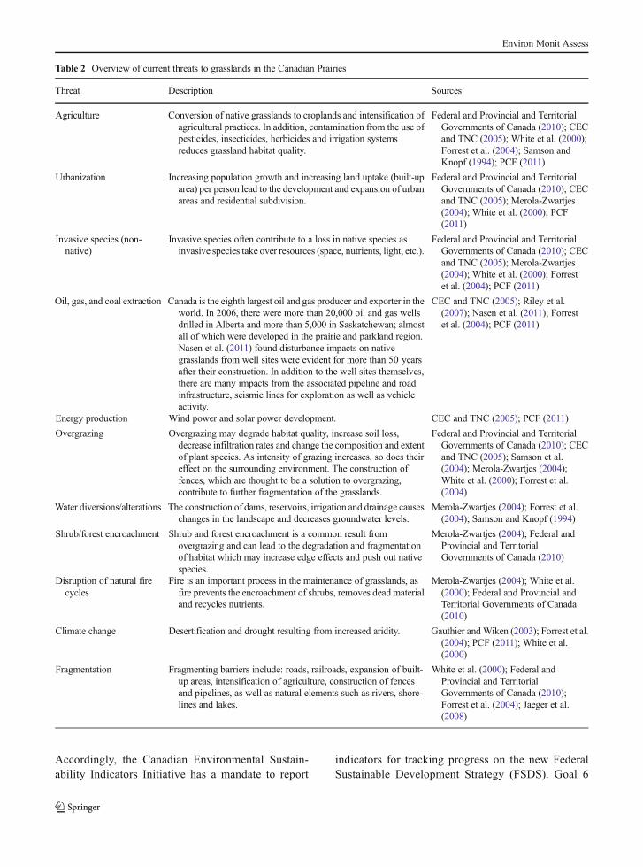
Table 2 Overview of current threats to grasslands in the Canadian Prairies

Threat Description Sources

Agriculture Conversion of native grasslands to croplands and intensification ofagricultural practices. In addition, contamination from the use ofpesticides, insecticides, herbicides and irrigation systemsreduces grassland habitat quality.

Federal and Provincial and TerritorialGovernments of Canada (2010); CECand TNC (2005); White et al. (2000);Forrest et al. (2004); Samson andKnopf (1994); PCF (2011)

Urbanization Increasing population growth and increasing land uptake (built-uparea) per person lead to the development and expansion of urbanareas and residential subdivision.

Federal and Provincial and TerritorialGovernments of Canada (2010); CECand TNC (2005); Merola-Zwartjes(2004); White et al. (2000); PCF(2011)

Invasive species (non-native)

Invasive species often contribute to a loss in native species asinvasive species take over resources (space, nutrients, light, etc.).

Federal and Provincial and TerritorialGovernments of Canada (2010); CECand TNC (2005); Merola-Zwartjes(2004); White et al. (2000); Forrestet al. (2004); PCF (2011)

Oil, gas, and coal extraction Canada is the eighth largest oil and gas producer and exporter in theworld. In 2006, there were more than 20,000 oil and gas wellsdrilled in Alberta and more than 5,000 in Saskatchewan; almostall of which were developed in the prairie and parkland region.Nasen et al. (2011) found disturbance impacts on nativegrasslands from well sites were evident for more than 50 yearsafter their construction. In addition to the well sites themselves,there are many impacts from the associated pipeline and roadinfrastructure, seismic lines for exploration as well as vehicleactivity.

CEC and TNC (2005); Riley et al.(2007); Nasen et al. (2011); Forrestet al. (2004); PCF (2011)

Energy production Wind power and solar power development. CEC and TNC (2005); PCF (2011)

Overgrazing Overgrazing may degrade habitat quality, increase soil loss,decrease infiltration rates and change the composition and extentof plant species. As intensity of grazing increases, so does theireffect on the surrounding environment. The construction offences, which are thought to be a solution to overgrazing,contribute to further fragmentation of the grasslands.

Federal and Provincial and TerritorialGovernments of Canada (2010); CECand TNC (2005); Samson et al.(2004); Merola-Zwartjes (2004);White et al. (2000); Forrest et al.(2004)

Water diversions/alterations The construction of dams, reservoirs, irrigation and drainage causeschanges in the landscape and decreases groundwater levels.

Merola-Zwartjes (2004); Forrest et al.(2004); Samson and Knopf (1994)

Shrub/forest encroachment Shrub and forest encroachment is a common result fromovergrazing and can lead to the degradation and fragmentationof habitat which may increase edge effects and push out nativespecies.

Merola-Zwartjes (2004); Federal andProvincial and TerritorialGovernments of Canada (2010)

Disruption of natural firecycles

Fire is an important process in the maintenance of grasslands, asfire prevents the encroachment of shrubs, removes dead materialand recycles nutrients.

Merola-Zwartjes (2004); White et al.(2000); Federal and Provincial andTerritorial Governments of Canada(2010)

Climate change Desertification and drought resulting from increased aridity. Gauthier andWiken (2003); Forrest et al.(2004); PCF (2011); White et al.(2000)

Fragmentation Fragmenting barriers include: roads, railroads, expansion of built-up areas, intensification of agriculture, construction of fencesand pipelines, as well as natural elements such as rivers, shore-lines and lakes.

White et al. (2000); Federal andProvincial and TerritorialGovernments of Canada (2010);Forrest et al. (2004); Jaeger et al.(2008)


of the FSDS covers Ecosystem/Habitat Conserva-tion and Protection. Its objective is to “maintainproductive and resilient ecosystems with the capac-ity to recover and adapt; and protect in ways thatleave them unimpaired for present and future gen-erations” (Sustainable Development Office and En-vironment Canada 2010).

Relationship between landscape fragmentationand connectivity

Fragmentation is defined as “the breaking up of a hab-itat, ecosystem, or land use type into smaller parcels”(Forman 1995, p. 39; Schumacher and Walz 2000) andimplies a reduction in landscape connectivity, which isdefined as “the degree to which the landscape facilitatesor impedes movement among resource patches” (Tayloret al. 1993, p. 571). Landscape connectivity depends onlandscape composition and configuration, and on a spe-cies’movement ability and risk of mortality when mov-ing through the landscape (Tischendorf and Fahrig2000).

Research questions

This study addresses two research questions:

1. What data are available for long-term monitoring ofgrassland fragmentation in the Canadian Prairiesand how suitable are they?

2. What is the current degree of fragmentation of theCanadian prairie grasslands?

In addition, we explore the feasibility of determiningfragmentation for historic points in time and of continu-ing monitoring grassland fragmentation in the future.We also examine the applicability and utility of theeffective mesh size metric for monitoring grasslands.

How to measure fragmentation?

Data availability and suitability

We found 11 candidate datasets that provide atleast some information about the spatial distribu-tion of grasslands in the Canadian Prairies between1993 and 2011. We used eight suitability criteria,each of them mandatory or desirable: (1) regulartime step updates (e.g. every 5 years)—mandatory;

(2) complete coverage of the Canadian grass-lands—mandatory; (3) classes and definitions clearand consistent over time—mandatory; (4) classesand definitions consistent between provinces—de-sirable; (5) resolution consistent over time, for thefuture—mandatory, and for the past—desirable; (6)historical data available—desirable; (7) contains agrassland class—mandatory; and (8) distinguishesbetween native and non-native grassland—desir-able. We then assigned scores for total overallsuitability, total mandatory suitability, and totaldesirable suitability.

Fragmentation geometries and reporting units

A fragmentation geometry (FG) specifies all theelements of fragmentation that will be considered(Jaeger et al. 2008). We used four FGs (full listgiven in Table 3 and further details in A8, A9,and A10 in ESM) that cover a range in landcovers, with increasing restrictiveness of the defi-nition of grassland from FG1 to FG4 in order togauge the uncertainty of our findings about grass-land fragmentation, as there are some variations inthe definitions of the land cover types that areconsidered “grassland” (Table 1). For example,the definition of grasslands by Gauthier and Wiken(2003) includes seeded tame pasture and aban-doned farm areas as grassland areas. Therefore,we created this array of FGs, which provide dif-ferent combinations of land covers that could pos-sibly include some type of grasslands. Anotherbenefit of using several FGs is they are applicableto a range of species, e.g. from habitat specialistswhich can only live in grassland habitat in a strictsense (FG4) to habitat generalists which can livein a wider range of habitats (FG1). An example ofa habitat specialist is the Sprague’s Pipet whorequires specifically native grasslands, whereasthe Loggerhead Strike is a habitat generalist whouses a wide variety of habitats: grasslands, pas-tures, shrubland, and even some agricultural areas(Parks Canada 2009; SARA 2010; COSEWIC2010).

We report the degree of fragmentation for the 7ecoregions, 17 sub-basins, 108 watersheds, 1,166 mu-nicipalities, and 50 census divisions located within thePrairie Ecozone, which we call “reporting units”.


Tab

le3

GIS

layersincluded

inthefourfragmentatio

ngeom

etriesused

inthisstudy.Forafulllistand

descriptionoftheCanVec

andAAFC

barriersincluded

inthefourFG

sseeA8,A9,and

A10.T

henumbersin

bracketsindicatethegrid

code

oftheclassesin

theAAFCdataset

Num

berandnameof

thefragmentatio

ngeom

etry

Definition

andrelevance

Two-dimensionalfeatures

One-dim

ensionalfeatures

AAFC’scrop

type

mapping

ofthe

prairies

CanVec

CanVec

Not

considered

asbarriers

Barriers

considered

Barriersconsidered

inallfourFGs

Barriersconsidered

inallfourFGs

FG1:Broad

grassland

fragmentatio

nIncludes

severalo

therland

covertypesin

additio

nto

thegrasslands

class;in

orderto

incorporateallp

ossibleland

coverswhich

may

berelatedto

grasslands

basedon

thevarious

definitio

nsof

land

covertypeswhich

may

ormay

notinclude

grasslands.

ThisFG

would

demonstratea

minim

umlevelo

ffragmentatio

nbecauseitprovides

aconservativ

eestim

ationof

therealfragmentatio

nas

therealfragmentatio

nisprobably

higher

dueto

barriersthatarenot

representedin

theavailabledatasets

anddueto

theinclusionof

otherland

covertypesnotspecifically

definedas

grassland.The

realdegree

ofgrassland

fragmentatio

nisatleastashigh

asthis

estim

ate.

Grassland

(110)

Wetland

(80)

Shrubland(50)

Hay/pasture

(122)

Fallo

w(131)

Allotherland

covertypes

Buildingstructures:

Buildings,tanks,residentialareas,

transformer

stations

andgasandoil

facilities

Hydrology:

Perm

anentsnowandice

Industrial

andcommercial

areas:

Mines,extractionareas,industrialand

commercialareas,industrialsolid

depots,dom

estic

waste,peatcuttin

g,quarries,autowreckers,pitsand

lumberyards.

Placesof

Interest:

Picnicsites,campgrounds,cem

eteries,

drive-in-theatres,lookouts,ruins,

sportstrack/race

tracks,golfdriving

ranges,park/sportsfields,amusem

ent

parks,forts,stadiums,zoos,golf

courses,exhibitio

ngrounds

Transportatio

n:Runways

Water

body:

Allwater

bodies

(exceptd

itches):canals,

lakes,reservoirs,w

atercourses,tid

alrivers,ponds,liquidwasteandside

channels.

Walls/fences

Manmadehydrographicentities

Sportstracks/racetracks

Railways

Cutlin

esCanals

Allroad

segm

ents(exceptw

inter

roads):freew

ays,expressw

ays/

highways,arterial,collectors,local,

alleyw

ays/lanes,ramps,resource/

recreatio

nandrapidtransitservice

lanes

FG2:

Fragm

entatio

nof

grassland,

wetland,shrubland

andhay/pasture

ThisFGissimilarto

FG1,in

thatit

includes

otherland

covertypesthatare

closelyrelatedto

grasslands

orcould

also

beclassified

asgrasslands

(pasture

insomedatasetsaregroupedinto

their

definedgrasslandclass).T

heonly

difference

betweenFG1andFG

2is

that“fallow”isconsidered

abarrierfor

FG2.

Grassland

(110)

Wetland

(80)

Shrubland(50)

Hay/pasture

(122)

Fallo

w(131)

Allotherland

covertypes

FG3:

Fragm

entatio

nof

grassland,

wetland

and

shrubland

ThisFG

provides

aninterm

ediatelevelof

grasslandfragmentatio

nas

itincorporates

noto

nlygrasslands

but

otherland

covertypeswhich

are

closelyrelatedto

grasslands

andare

less

likelyto

beabarrierformost

Grassland

(110)

Wetland

(80)

Shrubland(50)

Fallo

w(131)

Hay/pasture

(122)

Allotherland

covertypes


Tab

le3

(contin

ued)

Num

berandnameof

thefragmentatio

ngeom

etry

Definition

andrelevance

Two-dimensionalfeatures

One-dim

ensionalfeatures

AAFC’scrop

type

mapping

ofthe

prairies

CanVec

CanVec

Not

considered

asbarriers

Barriers

considered

Barriersconsidered

inallfourFGs

Barriersconsidered

inallfourFGs

grasslandspeciesas

theseland

cover

typesarestill

quite

natural.Unlike

FG1,thisFG

does

notinclude

any

agricultu

ralland(e.g.fallowor

pasture).

The

values

ofthisFGwould

fallbetween

thefragmentatio

nlevelsof

FG1and

FG4,therebyprovidingamedium

degree

offragmentatio

n.FG4:

Strictg

rassland

fragmentatio

nDescribes

grasslandfragmentatio

nin

anarrow

sense,as

thegrasslandclassis

theonly

AAFCland

useclassthatwas

notconsideredas

abarrier.Allother

land

covertypeswereassumed

tobe

abarrier.

ThisFG

representsthemaxim

umdegree

offragmentatio

n(relativeto

the

particular

datasetsused

andtheyear

beinganalyzed).The

realdegree

ofgrasslandfragmentatio

nmay

beless

than

thisestim

ate,sincetheremay

besomegrasslandincluded

inotherland

covertypesotherthan

inthe

“grassland”class.

Grassland

(110)

Fallo

w(131)

Hay/pasture

(122)

Wetland

(80)

Shrubland(50)

Allotherland

covertypes


Effective mesh size and effective mesh density

Various landscape metrics have been suggested in theliterature for quantifying fragmentation (e.g. Gustafson1998; Leitão et al. 2006). Their behaviour needs to becarefully studied before they are applied (Jaeger 2000,2002; Li and Wu 2004). We illustrate this by comparingfour metrics with the effective mesh size (meff) based ontheir behaviour in the phases of shrinkage and attritionof habitat patches which contribute to landscape frag-mentation (Forman 1995; Fig. 1). This example showsthat the average patch size, the number of remainingpatches, the number of large undissected low-trafficareas >100 km2, and the density of transportation linesdo not behave in a suitable manner in the phases ofshrinkage and attrition (Fig. 1). Therefore, their suitabil-ity is limited, whereas the meff behaves as desired.

The meff metric is based on the probability thatany two points chosen randomly in a region areconnected, i.e. are located in the same patch (Jae-ger 2000). This can be interpreted as the probabil-ity that two animals, placed in different locationssomewhere in a region, can find each other withinthe region without having to cross a barrier suchas a road or urban area. By multiplying this prob-ability by the total area of the reporting unit, it isconverted into the size of an area, which is calledthe effective mesh size. The smaller the meff, themore fragmented the landscape. The largest possi-ble value of meff is the size of the landscapestudied when the landscape is unfragmented. Thesmallest value of 0 km2 indicates complete frag-mentation, i.e. no suitable area left. This leads tothe formula:

meff ¼ A1

Atotal

� �2

þ A2

Atotal

� �2

þ A3

Atotal

� �2

þ…þ An

Atotal

� �2 !

⋅Atotal ¼ 1

Atotal

Xi¼1

n

A2i ; ð1Þ

where n is the number of patches, A1 to An represent thesizes of patches 1 to n, and Atotal is the area of thereporting unit.

The meff has highly advantageous properties,e.g. meff is relatively unaffected by the inclusionor exclusion of small or very small patches, and issuitable for comparing the fragmentation of re-gions of differing total areas and with differentproportions occupied by the barriers. Its reliabilityhas been confirmed through a systematic compar-ison with other quantitative measures based onnine suitability criteria (Jaeger 2000, 2002; Girvetzet al. 2007). The suitability of other metrics waslimited as they only partially met the criteria.

An important strength of meff is that it describes thespatial structure of a network of barriers in an ecologi-cally meaningful way that is easy to understand (Girvetzet al. 2007). Landscape-level ecological processes asso-ciated with species movements, such as foraging, dis-persal, genetic connectivity, and meta-population

dynamics, all depend on the ability to move throughthe landscape. Themeff is a direct quantitative expressionof landscape connectivity, as meff corresponds with theproposed measurement of landscape connectivity byTaylor et al. (1993): ‘landscape connectivity can be mea-sured for a given organism using the probability ofmovement between all points or resource patches in alandscape’. As a consequence, meff has substantial ad-vantages, e.g. it meets all scientific, functional, and prag-matic requirements of environmental indicators (see Jaegeret al. 2008 for a systematic assessment ofmeff based on 17selection criteria for indicators for monitoring systems ofsustainable development). Alternatively, the degree offragmentation can be expressed as the effective mesh den-sity seff=1/meff, i.e. the effective number of patches per1,000 km2 (Jaeger et al. 2007, 2008; Fig. 2).

We used the cross-boundary connections (CBC) pro-cedure to remove any bias due to the boundaries of thereporting units by accounting for the connections withinpatches that extend beyond the boundaries of the


Calculations:

APS = (sum of four patches / 4),followed by a jump to APS = (sum of three patches / 3).

Number of patches:

n = 4, then changes abruptly to n = 3.

No patches that are larger than 100 km2, thus nUDA100

does not capture the changes in the landscape.

The length of the roads stays constant at

2 * 4 km / 16 km2 = 0.5 km/km2.

The value of meff decreases continuously.

0.5 km/km2

0.25 km/km2

0 km/km2

Fig. 1 Illustration of the behaviour of four landscape metrics inthe phases of shrinkage and attrition of the remaining parcels ofgrassland due to the growth of an urban area. First row change ofthe landscape over time (black lines highways, black area resi-dential or commercial area; size of the landscape= 4 km×4 km=16 km2). Only the effective mesh size behaves in a suitable way

(bottom diagram). APS and n both exhibit a jump in their values(even though the process in the landscape is continuous);DTL andnUDA100 do not respond to the increase in fragmentation (meff

effective mesh size, n number of patches, APS average patch size,nUDA100 number of large undissected low-traffic areas >100 km2,DTL density of transportation lines)


reporting units (Moser et al. 2007). However, we ap-plied the cutting out (CUT) procedure along the outerboundaries of the Prairie Ecozone, i.e. only patchesinside this border were considered.

The meff can be split into two components: (a) pro-portion of habitat and (b) habitat fragmentation per se,where “habitat” refers to grassland or suitable area

(Atotal suitable ¼ ∑i¼1

nAi ). Their multiplication results in

meff:

meff ¼ 1

Atotal landscape

Xi¼1

n

A2i

¼ Atotal suitable

Atotal landscape⋅

1

Atotal suitable

Xi¼1

n

A2i

¼ Atotal suitable

Atotal landscape⋅ meff per se;

with

meff per se ¼ 1

Atotal suitable

Xi¼1

n

A2i ; ð2Þ

where Atotal suitableAtotal landscape

is the proportion of suitable area in the

reporting unit, and meff_per_se is the degree of grassland

fragmentation per se, i.e. it measures the probability thattwo points chosen randomly within grassland patchesare connected (not including locations outside of grass-land patches) and thus is conceptually independent ofhabitat amount. We used ArcGIS 9.3 (ESRI 2008) andtwo tools (one for creating the FGs and one for calcu-lating meff).

Results

Data suitability

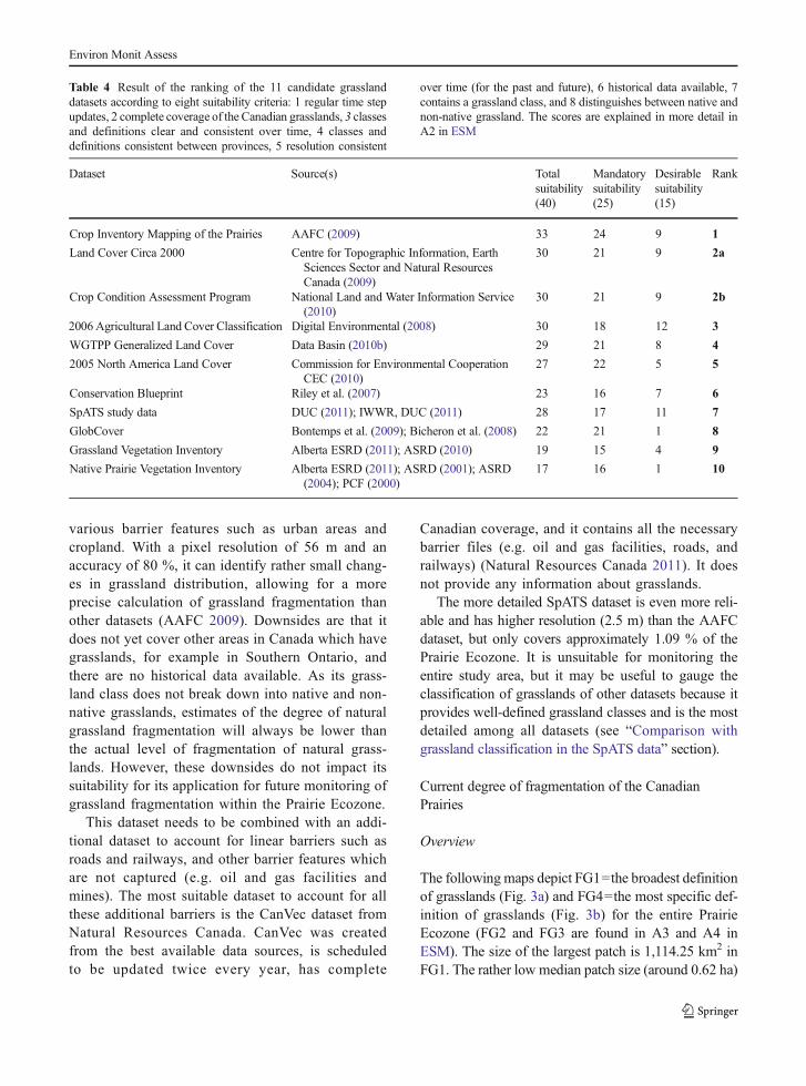
With a score of 33 out of 40 (mandatory 24/25 anddesirable 9/15), the Crop Inventory Mapping of thePrairies provided by Agriculture and Agri-Food Can-ada (AAFC) is the best dataset to use for monitoring(Table 4; full rating scores in A2 of ESM). It isexpected to be updated annually and has the long-term objective of expanding agricultural mapping tothe entire extent of Canada (making it highly suit-able for future monitoring), it has consistent classesand resolution over time and space; distinguishesgrasslands from other land cover types such as fal-low, shrubland, and hay/pasture; and includes

0

10

20

30

40

50

60

70

80

90

100

1940 1960 1980 2000 2020

Year

Effective mesh size, meff (km2)

0

5

10

15

20

25

30

35

40

45

50

1940 1960 1980 2000 2020

Year

Effective mesh density, seff

(meshes per 1 000 km2)

Fig. 2 Example illustrating the relationship between effectivemesh size and effective mesh density (effective number of meshesper 1,000 km2). In this hypothetical example, the trend remainsconstant. A linear rise in effective mesh density (right) corre-sponds to a 1/x curve in the graph of the effective mesh size (left).

A slower increase in fragmentation results in a flatter curve foreffective mesh size, and a more rapid increase produces a steepercurve. It is therefore easier to read trends off the graph of effectivemesh density (right)


various barrier features such as urban areas andcropland. With a pixel resolution of 56 m and anaccuracy of 80 %, it can identify rather small chang-es in grassland distribution, allowing for a moreprecise calculation of grassland fragmentation thanother datasets (AAFC 2009). Downsides are that itdoes not yet cover other areas in Canada which havegrasslands, for example in Southern Ontario, andthere are no historical data available. As its grass-land class does not break down into native and non-native grasslands, estimates of the degree of naturalgrassland fragmentation will always be lower thanthe actual level of fragmentation of natural grass-lands. However, these downsides do not impact itssuitability for its application for future monitoring ofgrassland fragmentation within the Prairie Ecozone.

This dataset needs to be combined with an addi-tional dataset to account for linear barriers such asroads and railways, and other barrier features whichare not captured (e.g. oil and gas facilities andmines). The most suitable dataset to account for allthese additional barriers is the CanVec dataset fromNatural Resources Canada. CanVec was createdfrom the best available data sources, is scheduledto be updated twice every year, has complete

Canadian coverage, and it contains all the necessarybarrier files (e.g. oil and gas facilities, roads, andrailways) (Natural Resources Canada 2011). It doesnot provide any information about grasslands.

The more detailed SpATS dataset is even more reli-able and has higher resolution (2.5 m) than the AAFCdataset, but only covers approximately 1.09 % of thePrairie Ecozone. It is unsuitable for monitoring theentire study area, but it may be useful to gauge theclassification of grasslands of other datasets because itprovides well-defined grassland classes and is the mostdetailed among all datasets (see “Comparison withgrassland classification in the SpATS data” section).

Current degree of fragmentation of the CanadianPrairies

Overview

The following maps depict FG1=the broadest definitionof grasslands (Fig. 3a) and FG4=the most specific def-inition of grasslands (Fig. 3b) for the entire PrairieEcozone (FG2 and FG3 are found in A3 and A4 inESM). The size of the largest patch is 1,114.25 km2 inFG1. The rather low median patch size (around 0.62 ha)

Table 4 Result of the ranking of the 11 candidate grasslanddatasets according to eight suitability criteria: 1 regular time stepupdates, 2 complete coverage of the Canadian grasslands, 3 classesand definitions clear and consistent over time, 4 classes anddefinitions consistent between provinces, 5 resolution consistent

over time (for the past and future), 6 historical data available, 7contains a grassland class, and 8 distinguishes between native andnon-native grassland. The scores are explained in more detail inA2 in ESM

Dataset Source(s) Totalsuitability(40)

Mandatorysuitability(25)

Desirablesuitability(15)

Rank

Crop Inventory Mapping of the Prairies AAFC (2009) 33 24 9 1

Land Cover Circa 2000 Centre for Topographic Information, EarthSciences Sector and Natural ResourcesCanada (2009)

30 21 9 2a

Crop Condition Assessment Program National Land and Water Information Service(2010)

30 21 9 2b

2006 Agricultural Land Cover Classification Digital Environmental (2008) 30 18 12 3

WGTPP Generalized Land Cover Data Basin (2010b) 29 21 8 4

2005 North America Land Cover Commission for Environmental CooperationCEC (2010)

27 22 5 5

Conservation Blueprint Riley et al. (2007) 23 16 7 6

SpATS study data DUC (2011); IWWR, DUC (2011) 28 17 11 7

GlobCover Bontemps et al. (2009); Bicheron et al. (2008) 22 21 1 8

Grassland Vegetation Inventory Alberta ESRD (2011); ASRD (2010) 19 15 4 9

Native Prairie Vegetation Inventory Alberta ESRD (2011); ASRD (2001); ASRD(2004); PCF (2000)

17 16 1 10


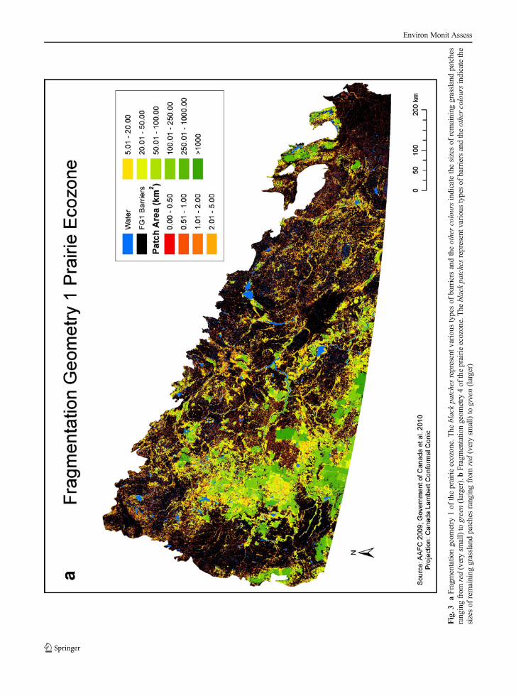
Fig.3

aFragm

entatio

ngeom

etry

1of

theprairieecozone.The

blackpatchesrepresentvarioustypesof

barriersandtheothercoloursindicatethesizesof

remaining

grasslandpatches

rangingfrom

red(verysm

all)togreen(larger).b

Fragmentatio

ngeom

etry

4of

theprairieecozone.The

blackpatchesrepresentvarious

typesof

barriersandtheothercoloursindicatethe

sizesof

remaining

grasslandpatchesrangingfrom

red(verysm

all)to

green(larger)


Fig.3

(con

tinu

ed)


indicates that there are many small patches andfew large patches of suitable area left. The sizesof these remaining patches strongly relate to thetotal land cover areas that are considered as po-tentially suitable areas (Table 5). The differencesbetween FG1 and FG4 demonstrate how includingthe land cover types of hay/pasture, shrubland,wetland, and fallow (FG1) in addition to only“grasslands” (FG4) affects grassland fragmentation.As FG1 includes the most land cover types assuitable, it seems natural to expect that it wouldexhibit the lowest level of fragmentation and thelargest remaining patch sizes, whereas FG4 wouldbe expected to exhibit the highest level offragmentation.

FG1 and FG2 are quite similar to each other in termsof the spatial distribution and sizes of the remainingpatches (as are FG4 and FG3). These similarities indi-cate that the addition or removal of fallow land as abarrier has rather little impact on the level of fragmen-tation, whereas the addition of hay/pasture as a barrierplays a much greater role (Table 4). Overall, manysmaller patches are located along the outer boundaryof the Prairie Ecozone in all FGs. Large patches are

concentrated in the lower sections of Saskatchewanand Alberta; most of them are found in the ecoregionsof Moist Mixed Grassland, Mixed Grassland, or Cy-press Upland. There are very few large patches in Man-itoba, with most patches located in the northern sectionof the Prairie Ecozone.

In Alberta, a major difference between FG1 and FG4is the higher number of small patches in the northernsection of the Prairie Ecozone in FG4. In fact, there arealmost no patches of grassland remaining here in FG4.In addition, the areas exhibiting a heavy concentrationof smaller patches in FG1 are further fragmented inFG4, and where there are larger areas (near the Sas-katchewan border in the centre and lower sections), thereduction in patch size is less pronounced. In Saskatch-ewan, a similar relation exists between FG1 and FG4:the northern section of the province is much morefragmented in FG4, also near the Manitoba border.The largest patches, located in the south-west of theprovince, next to the Alberta border, remain rather sim-ilar in both FGs. In Manitoba, the large patches in bothof the northern peninsulas in FG1 are almost completelyfragmented in FG4. In addition, the western side ofManitoba is much more fragmented in FG4. The

Table 5 Total land cover areas related to grassland for the PrairieEcozone, Alberta, Saskatchewan and Manitoba. In addition, themedian, minimum, and maximum values of the remaining patch

sizes of potentially suitable areas (i.e. grassland or related) consid-ered in the four FGs are listed

Total land-cover amount (km2)

Land cover type Prairie Ecozone Alberta Saskatchewan Manitoba

Fallow 13,847.558 1,172.163 12,216.203 459.193

Grassland 89,881.299 44,410.608 36,952.295 8,518.396

Hay/pasture 62,678.213 19,568.146 36,492.404 6,617.663

Shrubland 13,852.565 4,636.424 7,044.421 2,171.720

Wetland 9,947.429 3,432.846 4,233.499 2,281.084

FGs Prairie Ecozone Alberta Saskatchewan Manitoba

FG1 183,241.176 73,220.187 96,938.822 20,048.056

FG2 169,572.693 72,048.024 84,722.619 19,588.863

FG3 108,372.420 52,479.878 48,230.215 12,971.200

FG4 87,568.590 44,410.608 36,952.295 8,518.396

Amount of suitable area in the Prairie Ecozone (km2)

FG1 FG2 FG3 FG4

Sum 183,241.176 169,572.693 108,372.420 87,568.590

Median patch size 6.21E-03 6.18E-03 6.04E-03 6.26E-03

Min patch size 9.6E-12 9.6E-12 4.5E-12 2.9E-12

Max patch size 1,114.247 1,111.193 981.641 856.933


areas that experience little change are those on theeastern side of Manitoba; in FG1, there were al-ready hardly any patches left and those that remainare very small, and therefore, FG4 exhibits littlechange. These comparisons reveal the distributionand sizes of the remaining patches and show howthe consideration of different land cover typesinfluences this configuration.

The value of meff for the Prairie Ecozone in FG1 is25.44 km2. Considering the five classes: grassland, hay/pasture, fallow, shrubland, and wetland, there is183,241.176 km2 of suitable area left out of461,503.970 km2 (total area of the Prairie Ecozone).With the omission of fallow land in FG2, meff resultsin 24.67 km2, a 3.0 % decrease from FG1. When onlyconsidering the AAFC’s true grassland class, only87,568.590 km2 of grassland area remain, and FG4results in a much lower meff value of 14.23 km2, a44.1 % decrease from FG1. When shrubland and wet-lands are added, FG3 results in a considerably highervalue of meff=18.91 km2 (32.9 % higher; Table 7).

The meff are also measured for seven ecoregions(Table 7 and Fig. 5), 50 census divisions (Fig. 4 and 5;A5 in ESM), 1,166 municipalities (Fig. 5 and A12 inESM), 17 sub basins (Fig. 5 and A6 in ESM), and 108watersheds (Fig. 5 and A7 in ESM). The values (medi-an, min, and max values) for all four FGs are summa-rized in Table 6.

Ecoregions

The Southwest Manitoba Uplands region has the highestlevel of grassland fragmentation, indicated by the lowestvalues of meff, with meff=0.170 km2 in FG1 and meff=0.018 km2 in FG4. This ecoregion is primarily composedof forests and includes many lakes and ponds, but a ratherlow proportion of grasslands (337.19 km2 in FG1 and176.71 km2 in FG4 out of a total area of 2,183.44 km2).

The lowest levels of grassland fragmentation areobserved in the Cypress Upland, Mixed Grassland,and Fescue Grassland ecoregions, with the CypressUpland region exhibiting the highest values of meff of

Fig. 4 Distribution of the values of effective mesh size (in squarekilometers) for each of the four fragmentation geometries in the 50census divisions in the prairie ecozone. Since the fragmentationgeometries are building on each other, the values of meff are

ordered: meff (FG1)≥meff (FG2)≥meff (FG3)≥meff (FG4). Theinset shows the 32 census divisions whose meff values are lowerthan 10 km2 in FG1


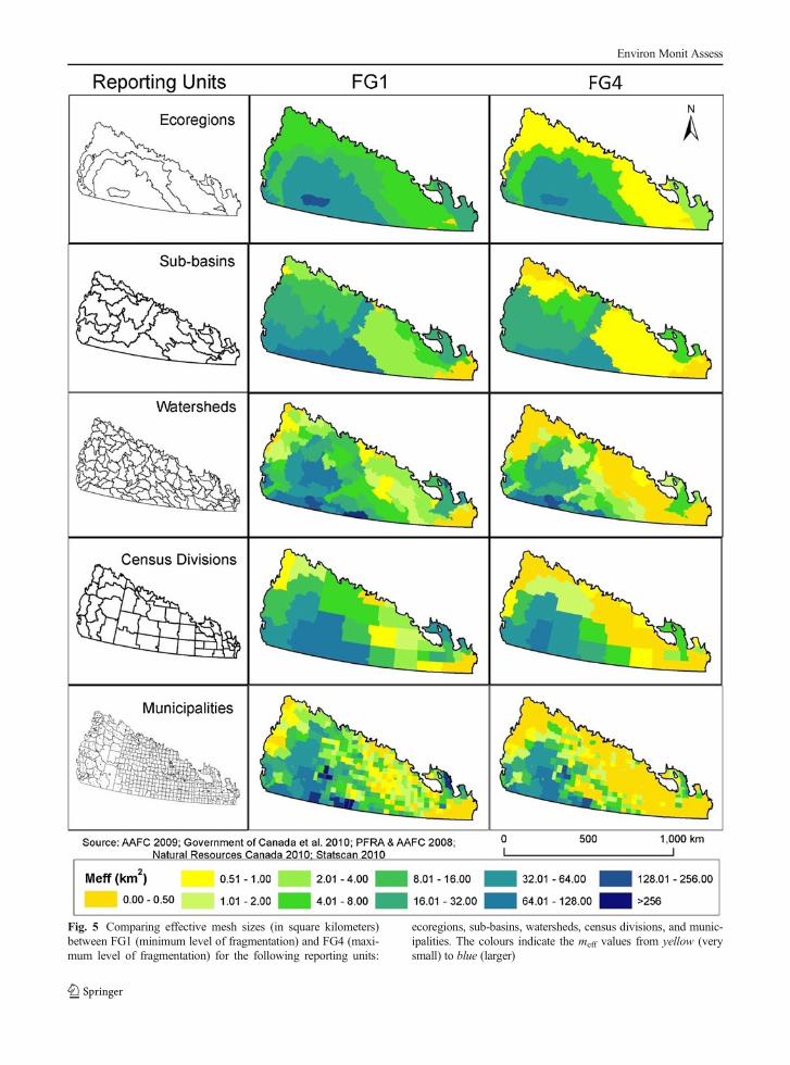
Fig. 5 Comparing effective mesh sizes (in square kilometers)between FG1 (minimum level of fragmentation) and FG4 (maxi-mum level of fragmentation) for the following reporting units:

ecoregions, sub-basins, watersheds, census divisions, and munic-ipalities. The colours indicate the meff values from yellow (verysmall) to blue (larger)


129.267 km2 in FG1 and 85.603 km2 in FG4 (the sameis observed for FG2 with meff=128.174 km2 and FG3with meff=116.476 km2). A major reason is that this iswhere most grasslands are located (6,574.48 km2 inFG1 and 5,305.28 km2 in FG4 out of 8,286.48 km2).However, the comparison of the meff values with thetotal area of grassland demonstrates that the grasslandsare highly fragmented even in these ecoregions.

Census divisions

Among the census divisions, the highest values of meff

are 99.085 km2 in FG1 and 77.034 km2 in FG4 (Figs. 4and 5). Both are observed in the census division (CD)4801, which is located to 15.4 % in the Cypress Uplandecoregion and to 84.6 % in the Mixed Grasslandecoregion. The second highest value is 84.174 km2 inFG1 for the CD 4815 and 49.307 km2 in FG4 for the CD4704 located east of CD 4801. CD 4704 is located to23.1 % in the Cypress Upland ecoregion and to 76.9 %in the Mixed Grassland ecoregion.

The lowest value of meff is 0.011 km2 in FG1 for the

CD 4610 (located in the south-east of the PrairieEcozone) and 0 km2 in FG4 for both the CDs 4809and 4813 (however, these CDs are located on the west

border of the Prairie Ecozone, the CUT procedure wasapplied along the Prairie Ecozone’s border, which couldinfluence these results). The next most heavilyfragmented grassland area for FG1 is found in CD4603 with a meff of 0.019 km2, and for FG4 in CD4811 with a meff of 0.001 km2. Interestingly, 26 CDsout of 50 fall into the 0–0.5 km2 meff category for FG4,whereas only 10 CDs fall into this category for FG1.This indicates that a large number of CDs are excessive-ly fragmented. In addition, all CDs exhibit a significantreduction in meff when comparing FG4 to FG1.

Municipalities

Among the 1,166 municipalities, one can observe grass-land fragmentation at a finer scale, giving the mostdetailed picture (Fig. 5). Three municipalities exhibiteither the highest or second highest meff values amongall four FGs: Mankota no. 45 (ID: 4703018) which islocated in the centre of Saskatchewan at the southernborder of the Prairie Ecozone with ameff of 380.227 km

2

in FG1, Pitville no. 169 (ID: 4708028) which is locatedin central Saskatchewan, near the Alberta border with ameff of 226.240 km

2 in FG4, and Clinworth no. 230 (ID:

Table 6 Reporting unit area and effective mesh size summarystatistics for the five types of reporting units: census divisions,municipalities, ecoregions, sub-basins, and watersheds. For eachtype of reporting unit, the median, minimum, and maximumeffective mesh size values are given for each of the four

fragmentation geometries. The reporting unit area for the wholePrairie Ecozone is 461,503.97 km2 and the effective mesh size ofthe Prairie Ecozone is 25.443 km2 for FG1, 24.669 km2 for FG2,18.912 km2 for FG3, and 14.233 km2 for FG4

Ecoregions Sub-basins Census divisions Watersheds Municipalities

Number of units 7 17 50 108 1,166

Reporting unit area (km2) Median 29,529.875 28,538.559 7,413.911 4,085.551 4.998

Min 2,183.440 11.444 1.330 0.206 0.109

Max 174,122.274 58,577.122 22,787.467 15,376.294 13,488.740

FG1 meff (km2) Median 20.411 5.250 4.425 3.610 0.250

Min 0.170 0.100 0.011 0.006 0.000

Max 129.267 82.269 99.085 264.411 380.227

FG2 meff (km2) Median 20.408 4.284 4.171 3.330 0.227

Min 0.166 0.082 0.011 0.006 0.000

Max 128.174 80.295 96.760 262.794 378.045

FG3 meff (km2) Median 18.646 1.367 2.065 1.520 0.017

Min 0.032 0.000 0.000 0.000 0.000

Max 116.476 60.111 87.630 197.729 294.748

FG4 meff (km2) Median 5.802 0.877 0.447 0.765 0.005

Min 0.018 0.000 0.000 0.000 0.000

Max 85.603 51.350 77.034 131.094 226.240


4708053) located in Saskatchewan above Pitville no.169 with a meff of 209.453 km2 in FG2.

In terms of the highest fragmentation level, all fourgeometries exhibit at least somemeff values of zero. FG1displays 41 municipalities, FG2 displays 51 municipal-ities, FG3 displays 192 municipalities, and FG4 393municipalities that have a meff value of 0 km2.

There are striking similarities between FG1 and FG4 interms of the minimum and maximum levels of fragmen-tation observed. Themunicipalities where fragmentation isthe lowest are generally the same for both geometries, andare located within the Mixed Grassland ecoregion. Theregions further away from this ecoregion have a greaternumber ofmunicipalities with higher fragmentation levels.For FG4 in particular, most municipalities along the outerborder of the Prairie Ecozone exhibit lowmeff values in therange of 0.0–0.5 km2. Both geometries also indicate a highdegree of fragmentation in the south-east of Manitoba,with very little suitable area remaining.

The northern section of Manitoba is significantlymore fragmented in FG4 than in all other FGs. This isespecially evident at the municipality scale in the small-er of the two peninsulas. However, the whole province isextremely fragmented in FG4, with many meff values inthe range of 0.0–0.5 km2. There are almost no grass-lands remaining in Manitoba.

Sub-basins

The meff values of the 17 sub-basins provide a broad-scale picture of fragmentation. For both FGs, sub-basin11A is the least fragmented, with ameff of 82.269 km

2 forFG1 and ameff of 28.463 km

2 for FG4. The highest levelof fragmentation is observed in two different regions withmeff=0.10 km2 in 05S for FG1 and meff=0 km2 in 07Bfor FG4. There are remarkable differences between FG1and FG4 (Fig. 5) for the sub-basins of 05J (meff=3.069 km2 for FG1 and meff=0.677 km2 for FG4), 05N

Fig. 6 Box and whisker plots showing the distribution of thevalues of the effective mesh size (in square kilometers) accordingto the fragmentation geometries FG1 and FG4, for the reportingunits of census divisions (CD), ecoregions (ER), municipalities(MUN), sub-basins (SB), and watersheds (WAT). FG1 depicts thebroadest definition of grasslands (minimum degree of fragmenta-tion) and FG4 the most specific definition of grasslands, i.e. for the

“grasslands” class only (maximum degree of fragmentation).Therefore, the meff values in FG4 are always smaller than inFG1. The dark lines in the middle of the boxes represents themedian, the bottom edge of the boxes represents the 25% quantile,the top edge of the boxes represent the 75 % quantile, the whiskersrepresent the 5 and 95 % quantiles, and the circles representsoutliers beyond the 5 and 95 % quantiles


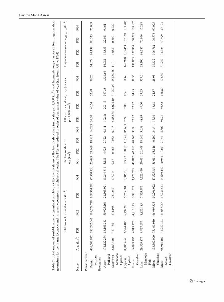
Tab

le7

Totalamountof

suitablearea

(i.e.grassland

orrelated),effectiv

emeshsize,effectiv

emeshdensity

(inmeshesper1,000km

2),andfragmentatio

nperse

forallfourfragmentatio

ngeom

etries

forthePrairieEcozone

andits

sevenecoregions

inalphabeticalorder.The

FGsareorderedin

orderof

decreasing

valueof

meff(i.e.from

FG1to

FG4)

Totalamount

ofsuitablearea

(km

2)

Effectiv

emeshsize:

meff(km

2)

Effectivemeshdensity:s

eff(m

eshes

per1,000km

2)

Fragmentatio

nperse:m

eff_per_se(km

2)

Nam

eArea(km

2)

FG1

FG2

FG3

FG4

FG1

FG2

FG3

FG4

FG1

FG2

FG3

FG4

FG1

FG2

FG3

FG4

Prairieecozone

Prairie

ecozone

461,503.972

183,242.042

169,574.738

108,374.280

87,570.450

25.443

24.669

18.912

14.233

39.30

40.54

52.88

70.26

64.079

67.138

80.535

75.009

Ecoregions

Aspen

Parkland

174,122.274

53,165.343

50,925.264

21,503.921

11,244.814

5.185

4.923

2.722

0.611

192.86

203.13

367.38

1,636.66

16.981

16.833

22.041

9.461

Southw

est

Manitoba

Uplands

2,183.440

337.186

334.198

233.245

176.714

0.17

0.166

0.032

0.018

5,882.35

6,024.10

3,1250.00

55,555.56

1.101

1.085

0.300

0.222

Cypress

Upland

8,286.484

6,574.485

6,497.981

5,755.681

5,305.281

129.27

128.17

116.48

85.603

7.74

7.80

8.59

11.68

162.928

163.453

167.691

133.706

Fescue

Grassland

14,899.793

4,913.175

4,913.175

3,991.522

3,423.755

43.812

43.812

40.245

31.9

22.82

22.82

24.85

31.35

132.865

132.865

150.229

138.825

Lake

Manitoba

Plain

29,529.875

8,837.685

8,825.185

7,859.587

5,223.430

20.411

20.408

18.646

3.058

48.99

49.00

53.63

327.01

68.200

68.287

70.056

17.288

Mixed

Grassland

133,567.000

75,460.930

66,989.835

50,296.922

47,525.454

55.611

53.546

40.209

34.541

17.98

18.68

24.87

28.95

98.432

106.762

106.778

97.075

Moist

Mixed

Grassland

98,915.107

33,952.373

31,087.056

18,731.543

14,669.142

10.964

10.693

7.764

5.802

91.21

93.52

128.80

172.35

31.942

34.024

40.999

39.123


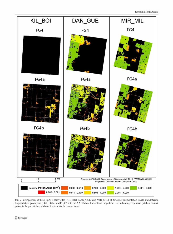
Fig. 7 Comparison of three SpATS study sites (KIL_BOI, DAN_GUE, and MIR_MIL) of differing fragmentation levels and differingfragmentation geometries (FG4, FG4a, and FG4b) with the AAFC data. The colours range from red, indicating very small patches, to darkgreen for larger patches, and black represents the barrier areas


(meff=3.340 km2 for FG1 and meff=0.877 km2 for FG4)and 05M (meff=5.250 km

2 for FG1 and meff=0.851 km2

for FG4). These are situated in the eastern side of Sas-katchewan near Manitoba. Another region exhibitinglarge decreases includes the sub-basins 05F (meff=10.518 km2 for FG1 and meff=0.925 km2 for FG4) and05E (meff=2.891 km2 for FG1 and meff=0.053 km2 forFG4) located at the northern peak of Alberta.

Watersheds

Watersheds provide a more detailed portrayal as theysubdivide the larger sub-basins. Comparing the highestand lowest meff values between FG1 and FG4 (Fig. 5)shows how considering different land cover types influ-ences the location of high and low fragmentation levels.The lowest fragmentation is found in the watershed(WS) 11AE for FG1, where meff=264.411 km2, andthe second lowest in WS 11AB for FG4, where meff=131.094 km2. The WS exhibiting the highest fragmen-tation in FG1 isWSWATwithmeff=0.006 km

2, followedby a meff=0.007 km2 in WS 05OD. In FG4, the lowestmeff observed is 0 km2 (i.e. complete fragmentation) infive watersheds: 07BC, 05GF, 07BB, 05DE, and WAT.The box and whisker plots illustrate how the distributionsof meff values differ among the reporting units (Fig. 6).

Partitioning fragmentation into proportion of suitablearea and fragmentation per se

The two components of meff are proportion of grassland(or suitable area) and grassland fragmentation per se(“Effective mesh size and effective mesh density”

section; Eq. 2). For example, themeff value of the PrairieEcozone of 14.233 km2 in FG4 can be partitioned intothe two components:

Atotal suitable

Atotal landscape¼ 87; 570:45 km2

461; 503:972 km2 ¼ 18:97%

and meff per se ¼ Atotal landscape

Atotal suitable⋅ meff

¼ 461;503:972 km2

87;570:45 km2 ⋅14:233 km2

¼ 75:01 km2

using the values from Table 7. Similarly, the value ofmeff=25.443 km2 in FG1 is the product of the twocomponents

Atotal suitable

Atotal landscape¼ 183; 242:042 km2

461; 503:972 km2 ¼ 39:71%

and meff_per_se=64.079 km2, indicating that the degreeof fragmentation per se of remaining suitable area isactually higher in FG1 than in FG4.

Comparison with grassland classification in the SpATSdata

The SpATS data distinguish “natural grassland” and“planted grassland” (IWWR, DUC 2011). SpATS de-fines “natural grassland” as “a mixture of native andtame grasses, forbs and shrubs that were not planted.Species occur either naturally or invaded. All wetlandmargins, most “native” pastures and roadside ditcheswould be considered natural grasslands” (IWWR,

Table 8 Comparing effective mesh size and effective mesh den-sity of FG4 with FG4a and FG4b for three SpATS study sites(using the CUT method). The suitable areas in FG4 are from theclass “grasslands” in the AAFC dataset. The suitable areas forFG4a are all grasslands classified in the SpATS data. For FG4b,

the only suitable areas are from the “natural grassland” class in theSpATS data. CanVec barriers have been included in all FGs (NSALno suitable area left, i.e. meff=0 km2, which would correspond toan infinite value of seff)

SpATS comparisons

Total amount of suitablearea (km2)

Effective mesh size:meff (km

2)Effective mesh density: seff (meshes per1,000 km2)

Study site Province Area (km2) FG4 FG4a FG4b FG4 FG4a FG4b FG4 FG4a FG4b

DAN_GUE_2008 AB 41.746 10.257 18.027 14.262 1.080 1.557 0.987 925.983 642.065 1,013.597

KIL_BOI_2008 MB 43.266 0.000 4.012 2.536 0.000 0.033 0.006 NSAL 29,855.178 154,800.091

MIR_MIL_2008 SK 42.276 22.303 21.641 18.326 2.483 2.222 1.837 402.811 450.139 544.399


DUC 2011, p. 123) and “planted grassland” as “areasseeded to grasses. Most planted grasslands are used forgrazing” (IWWR, DUC 2011, p. 123). After 2009, theSpATS dataset break down their grassland class evenfurther into native, planted, and other grassland. How-ever, since the AAFC data date from 2009, we decidedto compare the AAFC data with the 2008 SpATS data.

Comparing three study sites of differing fragmenta-tion levels allowed us to explore how a more detaileddefinition of grasslands influences the resulting degreeof fragmentation. It also reveals how close these twodatasets are in their mapping of grasslands in the PrairieEcozone. SpATS has a much finer resolution of 2.5 mcompared to 56 m for the AAFC data. The first studysite selected (DAN_GUE_2008) is located in Saskatch-ewan in an area of high grassland fragmentation in FG4.The second site (KIL_BOI_2008) is from Manitoba,with no grassland present according to FG4. The thirdsite (MIR_MIL_2008) is in a part of Alberta wheregrassland fragmentation is low according to FG4(Fig. 7).

We created two FGs using the SpATS data. The firstFG, called FG4a, includes both natural and plantedgrasslands as the only suitable areas, correspondingclosely to the AAFC grassland class, as the AAFC datado not distinguish between natural and non-naturalgrasslands. The second FG, called FG4b, includes only“natural grasslands” as suitable area to observe thedifference in grassland fragmentation when solely con-sidering “natural grasslands” (for a full list of landcovers included in FG4a and FG4b see A11 in ESM).

The comparison between the SpATS and the AAFCdata demonstrates how the classification of grasslandsand the resolution of a dataset can impact the degree ofgrassland fragmentation (Table 8). Just with these threestudy sites, three different situations emerged. For theDAN_GUE_2008 study site, the meff in FG4 is in be-tween the values of FG4a and FG4b. However, for theKIL_BOI_2008 study site, the meff in FG4 is lower thanthe values of both FG4a and FG4b, while forMIR_MIL_2008 the meff in FG4 is higher than thevalues of both FG4a and FG4b. This result under-lines that FG4 provides only a best estimate of theactual degree of grassland fragmentation at the res-olution of 56 m, and that the true level of grasslandfragmentation at a finer scale could indeed be some-what lower or higher, assuming that the SpATS dataare more accurate (which is supported by the mapsin Fig. 7).

The differences between FG4a and FG4b indi-cate that there is significantly less grassland, andtherefore, a higher degree of grassland fragmenta-tion, when only considering “natural grasslands” assuitable area (FG4b). In all three study sites, themeff values were lower in FG4b than in FG4a. Forthe DAN_GUE_2008 study site, this decrease was0.570 km2, for KIL_BOI_2008 it was 0.027 km2,and for MIR_MIL_2008 it was 0.385 km2. Eventhough these differences may seem quite low, onehas to consider the size of these study regions(which are between 41 and 43 km2). If the SpATSdata covered the entire Prairie Ecozone, these dif-ferences would be notably greater.

Discussion

Indicators for detecting changes in grassland fragmen-tation in an efficient way are needed in order to applyappropriate and reliable management strategies beforethe remaining grassland patches may be forever lost orbecome degraded beyond repair (White et al. 2000).Understanding how grasslands have changed over timeand knowing their remaining extent and distributionallows for more informed and targeted conservationefforts. The quality of this information may depend tosome degree on the datasets and methods being used.The results of this study quantify for the first time thecurrent degree of fragmentation of the Canadian Prai-ries. Scientists and policy makers can now turn to thecontinued monitoring of grassland fragmentation, anddesign suitable conservation strategies.

Differences among regions

Comparisons among ecoregions reveal how the level ofgrassland fragmentation observed depends on their lo-cation. The Southwest Manitoba Uplands region (some-times erroneously referred to as “Boreal Transition” insome datasets) exhibits the highest level of grasslandfragmentation in all four FGs. The values of meff aremuch lower than the total amount of grassland area,which indicates their excessive degree of fragmentation.The lowest levels of grassland fragmentation (for allfour FGs) are found in the Cypress Upland, followedby the Mixed Grassland and Fescue Grasslandecoregions. The comparison of the meff values with thetotal area of grassland demonstrates that the grasslands


are highly fragmented even in these ecoregions, withecoregions having a greater proportion of grasslandsexhibiting a lower level of fragmentation.

Even though FG1 has more suitable area than FG4,the additional land cover types considered in FG1 are infact highly scattered throughout the Prairie Ecozone.Intuitively, one might expect that their inclusion wouldcreate larger patch sizes as mentioned in the “Currentdegree of fragmentation of the Canadian Prairies” sec-tion; however, this is often not the case. For example,Manitoba and the outer edges of the Prairie Ecozonehave many small patches of grasslands, but when addi-tional land covers are added as suitable area, they them-selves result in even tinier patches because they do notalways touch the grassland patches. Therefore, FG1 iscomprised of many more small patches of suitable areathan FG4, which results in a higher level of fragmenta-tion per se (and a lower meff_per_se value; Table. 7).Comparingmeff values between reporting units providesadditional insights into the degree of fragmentation. It isimportant to not only look at natural reporting units likeecoregions and watersheds but to also explore the an-thropogenic reporting units such as municipalities, asthese are more often referred to in political and policy-related activities. For different organizations, differentreporting units may be of interest and therefore it is bestto provide information for a number of reporting units tomeet the requirements of a range of organizations andtheir goals.

The values of meff are much lower than the totalamount of grassland/suitable area in all reporting unitsin all FGs, which indicates their extreme degree offragmentation. The question may arise what values offragmentation should be considered as “natural”, “un-disturbed”, “normal”, or “acceptable”. However, ourcomparisons of high and low fragmentation levels arebased on only one point in time (2009). Therefore, it isunknown what the “natural” level of fragmentationwould be. Further studies are required to tackle thisissue; but the lack of detailed historic maps of grasslandsmakes this task difficult (see “Feasibility of measuringgrassland fragmentation levels for historic points intime” section).

Comparison with other studies

The total area of the land cover type “grassland” in FG4is 87,570.45 km2 out of a possible area of461,503.97 km2, i.e. 18.98 % of the study area. The

corresponding percentages are 39.71 % for FG1,36.74 % for FG2, and 23.48 % for FG3 (Table 7),somewhat similar to estimates given in the literature.The study by the Federal, Provincial and TerritorialGovernments of Canada (2010) stated that mixed andfescue grassland cover over 110,000 km2. This is well inthe range provided by the four FGs from 87,570.45 km2

(FG4) to 183,242.04 km2 (FG1) of our study.Gauthier and Wiken (2003) estimated that 25–30 %

of the native grasslands remain in the Canadian prairiesand parklands. Our value of 87,570.45 km2 seen as the25–30 % estimate of remaining grasslands would implyan original total area between 148,869.76 and153,248.28 km2 for FG4 and between 309,811.46 and320,673.57 km2 for FG1, meaning that 69.48–67.13 %of the Prairie Ecozone was once covered by grasslands.However, the AAFC land cover data does not distin-guish between native and non-native grasslands. There-fore, this calculation cannot be done for the area ofnative grasslands alone.

Suitability of the effective mesh size/density methodfor monitoring grassland fragmentation

Indicators that are suitable for monitoring various eco-systems are in high demand. This is the first study toapply the meff method to grasslands. With that, ourresults have shown that the meff is highly suitable formeasuring grassland fragmentation due to its manystrengths (“Effective mesh size and effective mesh den-sity” section) and is therefore recommended for long-term monitoring of the grasslands in the Canadian Prai-ries. Many countries have already implemented meff orseff as an indicator for environmental monitoring. Someexamples are Switzerland (Bertiller et al. 2007; Jaegeret al. 2007, 2008), Germany (Schupp 2005; FederalMinistry for the Environment and Nature ConservationandNuclear Safety BMU2007), California (Girvetz et al.2008), South Tyrol (Tasser et al. 2008), Baden-Württemberg (State Institute for Environment, Measure-ments and Nature Conservation Baden-Württemberg2006), and on the European level (EEA and FOEN2011). Most recently, it has been included in the CityBiodiversity Index (CBI) (also called the Singapore Indexon Cities’Biodiversity) of the Conference of the Parties tothe Convention on Biological Diversity (Chan andDjoghlaf 2009) as an indicator of connectivity of naturalareas in cities on a global scale (CBI User Manual 2011/


12; Asgary 2012). It can also be used for the design ofhabitat networks in cities (Deslauriers 2013).

Other useful applications of the meff method are:exploring how new roads or urban areas or the remov-al of roads would affect the degree of grassland frag-mentation. The meff method can be extended to includethe permeability of barriers for animals moving in thelandscape (i.e. filter effect; Jaeger 2002, 2007) and canhelp indicate where the addition of a wildlife corridoror conservation area would be particularly beneficial tolandscape connectivity.

The difference between meff and meff_per_se denotesthe difference between the suitable area accessible onaverage to an individual being placed anywhere in thelandscape without having to cross a barrier (meff) andan individual being placed anywhere inside a patch ofsuitable area without crossing a barrier (meff_per_se).The addition of barriers can reduce or increase thevalue of meff_per_se, whereas the value of meff willalways be reduced. For example, loss of small grass-land patches will increase meff_per_se, indicating thatfragmentation per se has been reduced, but the grass-land area has decreased. The meff combines these twocomponents and decreases when grassland patches ofany size are lost. Changes in meff_per_se will thereforeonly be interpreted correctly as a positive or negativechange when the change in grassland amount is con-sidered at the same time. Changes in meff are easier tointerpret: a decrease in meff always indicates a higherlevel of fragmentation, due to either a breaking up ofpatches, or a loss of grassland area, or (usually) acombination of both. As a consequence, the values ofmeff are ordered as meff.FG1>meff.FG2>meff.FG3>meff.FG4, but this is not the case with meff_per_se. Formonitoring grassland fragmentation, all three valuesshould be reported (proportion of suitable area, meff,and meff_per_se) to be able to distinguish between habitatamount and fragmentation per se. Alternatively to meff

and meff_per_se, the respective effective mesh densities,seff ¼ 1

meffand seff per se ¼ 1

meff per secan be used, where

seff per se ¼ Atotal suitableAtotal landscape

⋅seff .

Feasibility of measuring grassland fragmentation levelsfor historic points in time

Historical data are of great interest for estimating pastrates of fragmentation increase and changes in trends.However, when accessible GIS data layers are updatedthe previous versions are usually not accessible any

more. There may be printed maps or aerial photographsavailable that include historic information. However,their use would require aerial photo interpretation anddigitization of historic maps (beyond the scope of thisstudy).

The oldest land cover dataset we found that is suit-able for calculating grassland fragmentation was theWGTPP Generalized Land Cover from 1993/95 (DataBasin 2010a). The next oldest is the Geobase 2000dataset (Centre for Topographic Information, Earth Sci-ences Sector and Natural Resources Canada 2009). Themain constraint for these two points in time is the lack ofadditional barrier data (e.g. road and railway data). AsCanVec does not have an archive system, it is currentlyimpossible to retrieve older datasets. Therefore, the bar-rier data used from CanVec do not go that far back. Infact, their first edition dates back to 2007. Therefore,comparisons without these barriers would not be mean-ingful. Another concern is that the changes over just15 years (between 1993/95 and 2009) may be too smallto be detected reliably. The most important changesoccurred before 1990 (and most significantly before1930). In addition, there are differences in resolution(in space and in land cover class definitions), whichcould make meaningful comparisons impossible. How-ever, hard paper topographic maps could be digitized oraerial photographs could be georeferenced to retrieveolder land cover, road, and railway data. Therefore, ahistorical analysis is in principle feasible in futurestudies.

Feasibility of monitoring grassland fragmentationin the future

The suitability assessment for the 11 grassland datasetsrevealed the combination of the Crop Inventory Map-ping of the Prairies and the CanVec dataset to be themost suitable for monitoring grassland fragmentation ifboth datasets continue to be updated in the same way(i.e. classes and spatial resolution) as is expected. There-fore, monitoring grassland fragmentation in the future isindeed possible and recommended.

The selection of the most appropriate FG for moni-toring generally depends on a study’s context and ob-jectives. The combination of all four FGs may be moreappropriate than any single FG. However, if all four FGscould not be considered for any particular reason, thenFG4 would be the most appropriate. In addition, FG1


may serve as a suitable representation of grassland frag-mentation in a broad sense.

Conclusions

Recommendations for controlling grasslandfragmentation

This study shows that the remaining grasslands in theCanadian Prairies are heavily fragmented. Therefore,conservation efforts need to focus on grasslands beforethey degrade further and their qualities are forever lost.There are various conservation initiatives currently inoperation that aim to protect remaining grassland areas.One of them on the national level is the CanadianCouncil on Ecological Areas (CCEA) that created theConservation Areas Reporting and Tracking System(CARTS) in March 2004 (CCEA 2010). This programhelps regularly and systematically track and report onthe status of Canada’s protected areas. Protected areasare defined in CARTS as: “a clearly defined geo-graphical space, recognized, dedicated and managed,through legal or other effective means, to achieve thelong-term conservation of nature with associated eco-system services and cultural values” (Vanderkam2010, p. 1). To determine to what degree theseprotected areas overlap with the remaining largepatches of grassland, we overlaid the CARTS regionswith the map of the remaining patches of grasslandhabitat and their fragmentation. This could indicatethe need for the creation of additional CARTS regionsto better control the degradation and fragmentation ofthe grasslands. In the Prairie Ecozone, there are 382conservation areas resulting in a total protected areaof only 21,038 km2 or 4.56 % of the total area of thePrairie Ecozone. Out of 25 ecozones in Canada, thePrairie Ecozone is the tenth lowest protected ecozone(Environment Canada 2011). The CARTS protectsonly 11.60 % of grassland area identified in FG4,representing 48.27 % of the total CARTS areas withinthe Prairie Ecozone.

The majority of the CARTS areas are located in theprovince of Saskatchewan. In Saskatchewan, the largergrassland patches are usually associated with a conser-vation area, which indicates that these CARTS areas arehelping limit grassland fragmentation and therefore,increasing the CARTS areas would prevent further deg-radation and fragmentation of these remaining grassland

patches. Alberta and Manitoba, however, have very fewCARTS regions and those that are present are rarelyassociated to a grassland area. Interestingly, some ofthe largest remaining grassland patches are located inAlberta, with only a few of these areas being protectedunder CARTS. Therefore, we recommend that theseCARTS areas be expanded considerably to cover sub-stantially more of the remaining patches of grasslandhabitat.

On a provincial basis, the Saskatchewan Repre-sentative Areas Network (RAN) Program wasestablished in 1997 by Saskatchewan Environment.The program once completed, will comprise a net-work of approximately 7.8 million hectares (or 12 %of the province of Saskatchewan). The RAN aims atconserving representative and unique landscapes inevery ecoregion within Saskatchewan. The majorgaps of these representative landscapes coincidewith the agricultural areas of the province, whichare located in the Mixed Grassland, Moist MixedGrassland, and the Aspen Parkland ecoregions.Challenges arise in establishing conservation areashere, especially in the Mixed Grassland and theMoist Mixed Grassland ecoregions as most of thisland has already undergone cultivation (80 % in theMixed Grassland ecoregion and 50 % in the MoistMixed Grassland ecoregion), or the land is privatelyowned or under long-term lease agreements (Sas-katchewan Environment 2005). Concerns of everbeing able to meet the 12 % protection targets forthese two ecoregions are high. These two ecoregionshave the highest amount of grassland area (in FG4).While the meff of the Moist Mixed Grassland regionis the highest among all the ecoregions (meff=34.541 km2), the Mixed Grassland ecoregion has ameff value of only 0.611 km2, i.e. it is the secondmost fragmented ecoregion (the most fragmented isthe Southwest Manitoba Uplands ecoregion). Thisdemonstrates the urgent need to protect these re-maining patches in the Moist Mixed Grasslandecoregion and the Mixed Grassland ecoregion be-fore they become further reduced in size and quality.

Even though these conservation initiatives are essen-tial and constitute an important step towards the protec-tion of remaining grasslands and other natural areas,they are clearly not sufficient to address all the threatsagainst the Prairie grasslands (Table 2) because they donot cover enough area and are not sufficiently supportedby regulations for grassland protection. Conservation


efforts should not only protect the remaining largeunfragmented areas, but also prevent further fragmenta-tion of areas where grasslands are already highlyfragmented to preserve biodiversity in these places aswell. The long response times of many species to chang-es in landscape structure present a particular challengeglobally (Tilman et al. 1994; Kuussaari et al. 2009;Dullinger et al. 2013). The current population densitiesmay not reflect their response to the current grasslandpatterns but to earlier grassland patterns decades ago,and wildlife populations may continue to decline formany years even when the degree of grassland fragmen-tation does not increase any more (Helm et al. 2006;Lindborg and Eriksson 2004). Given that many negativeeffects of habitat fragmentation and isolation only be-come apparent after several decades, further populationlosses will be incurred in the coming decades as a resultof the changes that have already taken place in the past(Findlay and Bourdages 2000).

The implementation of effective mesh size as anindicator of fragmentation for grassland monitoringand management is an increasingly pressing issue asthe degree of fragmentation in the Prairie Ecozone con-tinues to rise and the remaining grassland habitatpatches continue to decrease and disappear. A quantita-tive metric of grassland fragmentation can help set mea-surable targets or limits for regions or provinces to guidemanagement efforts; the meff (or seff) metric is highlysuitable for quantifying this indicator. We recommendthat the fragmentation values be updated on a regularbasis to document trends and detect changes in anytrends in grassland fragmentation.

As an example, what measures are suitable and fea-sible for bringing about a trend reversal in grasslandfragmentation caused by roads and other transportationinfrastructure? Generally, four types of measures can bedistinguished: (1) to minimise negative impacts duringthe planning and construction stages of new transporta-tion infrastructure, (2) to restore connectivity acrossexisting transportation infrastructure, (3) to prevent fur-ther increase of the density of the transportation net-work, and (4) to remove existing transportation infra-structure (EEA and FOEN 2011). Some useful measuresto curtail grassland fragmentation from roads are:

1. Existing roads can be made more permeable forwildlife through tunnels, wildlife crossings (over-passes and underpasses), or by raising roads up onpillars so that wildlife can cross underneath. In

general, the larger the areas linked together, themore effective the measures will be.

2. The widening of existing highways and higher traf-fic volumes will increase their barrier effect. How-ever, the upgrading of existing highways is still lessdetrimental than the construction of new highwaysat another location in most cases, even if the newhighways were to be bundled with existing trans-portation infrastructure. This has been demonstratedby a computer simulation model that determinedprobabilities of population persistence to comparethese alternatives (Jaeger et al. 2006).

3. If bypasses (and other roads) are sited close todeveloped areas, their fragmentation effect is lowercompared to bypasses away from settlements. Thepurpose of this measure is to preserve unfragmentedareas that are as large as possible and thereby lessenthe fragmenting impact of any new transport routes.

4. Transport infrastructure which is not urgently need-ed any more (e.g. due to the construction of newroutes or changing requirements) should be re-moved. This is particularly important whereexisting infrastructure is located in an area of animalmovement corridors, e.g. amphibian migrationcorridors.

5. Roads, on which traffic volumes have decreaseddue to the construction of other transportation infra-structure or due to changing conditions, should bedowngraded and physically reduced in width. Thismeans a reduction of their surface and their footprinton the ground through physical modification.

It is also necessary to limit the size of urban areassince built-up areas are themselves barriers to animalmovement, and because urban sprawl and road con-struction mutually intensify each other: dispersed pat-terns of settlement areas lead to higher traffic volumesand more road construction, and roads attract urbandevelopment. Regional planning legislation shouldmore effectively require local authorities to treat landsparingly in their land use plans. Regional and localauthorities should limit the growth of built-up areasand instead encourage denser development within theboundaries of existing urban areas.

Measures for controlling grassland fragmentation canonly be effective if there is an awareness of the problemand feasible solutions are proposed. Decision makers


and the general public should therefore be made moreaware of the problems of grassland fragmentation andhabitat loss and need to be informed about suitablemeasures. The setting of limits can play an importantrole for this objective. For example, specific targets,benchmarks, and limits could be distinguished accord-ing to the respective type of landscape such as: (1)priority regions for large unfragmented areas; i.e. nofurther fragmenting elements are allowed here, and thereis a priority for the removal of existing fragmentingelements, and (2) further fragmenting elements couldbe allowed in densely settled landscapes or along devel-opment axes up to a certain limit.

Our results can be used to set quantitative goals toprovide a comparative basis, which can be reviewedthrough environmental monitoring: The degree of frag-mentation can be recalculated after new roads have beenbuilt or existing roads have been removed, and com-pared to the targets or limits. This is already possible inthe planning stages of the construction or removal oftransportation infrastructure. Maps of planned transpor-tation infrastructure can be combined with models forpredicting future land use changes, and the resultingdegree of fragmentation can be compared to the target.Thus, the use of quantitative data about grassland frag-mentation as a tool for performance review of protectionefforts is an approach for increasing awareness andguiding efforts for minimising grassland fragmentation.Such analysis and performance review is applicablewith regard to both biodiversity and landscape quality.

Little is known about the exact fragmentation thresh-olds for the persistence of wildlife populations, and howthese thresholds will shift due to diminishing resources,reduced genetic exchange, or changes in climate (Robin-son et al. 2010). Other factors, such as the spatial distri-bution of habitats or changes in a population’s birth ormortality rates may also influence these thresholds. Aslong as the knowledge about the thresholds of the effectsof grassland fragmentation on wildlife populations andecosystem services is insufficient, the precautionary prin-ciple should be applied (Kriebel et al. 2001). A particularchallenge is given by the long response times of popula-tions of long-lived animals to changes in landscape struc-ture (Kuussaari et al. 2009). This situation makes it all themore essential that a precautionary approach is adoptedthat guides grassland fragmentation in the desired direc-tion. The lack of knowledge about the exact location ofthe thresholds should not be used as an argument forpostponing protective measures. Rather, targets and

limits for the future degree of landscape fragmentationshould be broadly discussed and implemented now. Suchtargets and limits are urgently needed by governmentoffices and administrations to be able to act and justifytheir decisions and actions towards better protection ofgrasslands. These limits cannot be set in stone but shouldbe region-specific and should consider the ecological,geographic, social, economic, and historic characteristicsof each region.

Future research needs

Future studies should broaden our understanding ofgrassland fragmentation in the Canadian Prairies basedon the results presented in this paper. Suggestions forsuch studies include the following:

1. To incorporate varying degrees of permeability ofbarriers within the current meff method. The proba-bility of successful barrier crossings and the positiveeffect of wildlife passages on landscape connectiv-ity can be included in a more detailed version of themeff (Jaeger 2007). This analysis would be based onthe habitat requirements and sensitivity to variousbarriers of a certain species (or a range of species).This could be particularly relevant for species whichare at risk of extinction as maintaining connectivityfor ecological processes is a prerequisite for theconservation of species in fragmented landscapes(McRae and Beier 2007).

2. To conduct a historical analysis of grassland frag-mentation for the Prairie Ecozone for multiple timesteps (e.g. every 10–20 years), potentially goingback to the 1930s or 1940s. This would reveal majorchanges in grassland fragmentation. It would entaillarge amounts of digitization and would be based onbarriers that are documented in historical maps.

3. To incorporate additional features such as pipelinesand transmission lines and to explore to what degreethey increase the level of grassland fragmentation;this is important as certain species can be impactedby these additional barriers, through either avoidingthese areas completely or being unable to moveacross these barriers. In addition, pipelines andtransmission lines can contribute to the degradationof grassland habitat quality, which may have similarecological repercussions as the direct removal ofgrasslands (e.g. reducing the probability of popula-tion persistence). These additional FGs may also be


relevant for humans in terms of landscape aestheticsand the recreational value of the landscape.

4. To compare the values of meff for all the locationsfor which SpATS data (120 study sites) are availablewith the Crop Inventory Mapping of the Prairiesdataset. This comparison would allow for a fine-scale analysis of grassland fragmentation that dis-tinguishes between native and non-native grass-lands. It would provide higher spatial and thematicresolution and higher accuracy for 1.09 % of thearea of the Prairie Ecozone.

All these efforts to improve the quality of the moni-toring, however, will only contribute to a trend reversalin grassland fragmentation if the data are actually usedfor increasing problem awareness and for implementingmore sustainable management policies than those thatare in place today.

Acknowledgments We gratefully acknowledge the contribu-tions of the following people who have provided valuable infor-mation and data: Mickey Currie (Alberta Sustainable ResourceDevelopment), ZuZu (Fawziah) Gadallah (Environment Canada),Scott Mitchell (Carleton University, Ottawa), John Riley (NatureConservancy of Canada), Susan Witherly (Ducks Unlimited),Patrick Rollin (Agriculture and Agri-Food Canada), Alexis Dorais(Univ. de Montréal) and David Beauchesne (Concordia Univ.Montréal). We also thank everyone who replied to our inquiriesabout available datasets, two anonymous reviewers for their con-structive comments, and Environment Canada for financialsupport.

References

Agriculture and Agri-Food Canada (AAFC) (2009). Metadata—crop inventory mapping of the Prairies. Earth ObservationUnit of the Agri-Environment Services Branch (AESB).[XML Document].

Alberta Environment and Sustainable Resource Development(ESRD). (2011). Forest & vegetation inventories. http://www.srd.alberta.ca/MapsPhotosPublications/Maps/ResourceDataProductcatalogue/ForestVegetationInventories.aspx. Accessed 15 Sept 2011

Alberta Sustainable Resource Development (ASRD) (2010).Grassland vegetation inventory (GVI) Specifications, 5thedition. pp. 90 [PDF].

Alberta Sustainable Resource Development (ASRD) (2004).Metadata—native prairie vegetation inventory (extended)Arc/Info Coverage. pp. 3.

Alberta Sustainable Resource Development (2001).Native Prairievegetation inventory for the prairie region—terms of refer-ence. pp. 5.

Asgary, A. (2012).Measuring the connectivity of natural areas inthe City Biodiversity Index (CBI) using the effective mesh size(meff). Unpublished Honour’s Thesis (p. 90). Canada:Department of Geography, Planning and Environment,Concordia University Montréal.

Bertiller, R., Schwick, C., & Jaeger, J. (2007). Degree of land-scape fragmentation in Switzerland: Quantitative analysis1885–2002 and implications for traffic planning and region-al planning. Project report (in German). FEDRO report No1175 (Swiss Federal Roads Authority), Berne, pp. 229.

Bicheron, P., Defourny, P., Brockmann, C., Schouten, L., Vancutsem,C., & Huc, M., et al. (2008).GLOBCOVER—products descrip-tion and validation report. Distributed by ESA. pp. 47 [PDF].

Bontemps, S., Defourney, P., & Van Bogaert, E. (2009).GLOBCOVER 2009—product description manual.Distributed by ESA. pp. 17 [PDF].

Canadian Council on Ecological Areas (CCEA). (2010).Conservation areas reporting and tracking system (CARTS).http://www.ccea.org/en_carts.html.

CBI User Manual. (2011/12). User’s manual for the City BiodiversityIndex. 13 October 2011/updated on 18 April 2012. 25 pp. http://www.cbd.int/authorities/gettinginvolved/cbi.shtml.

CEC and TNC. (2005). North American Central grasslands prior-ity conservation areas: technical report and documentation. InJ.W. Karl and J. Hoth (Eds.), Montreal: Commission forEnvironmental Cooperation and The Nature Conservancy.

Centre for Topographic Information, Earth Sciences Sector andNatural Resources Canada. (2009). Land cover, circa 2000-vector: Feature catalogue, edition 1.0. Geobase [PDF]. http://www.geobase.ca/geobase/en/data/landcover/csc2000v/description.html.

Chan, L., & Djoghlaf, A. (2009). Invitation to help compile anindex of biodiversity in cities. Nature, 460, 33. doi:10.1038/460033a.

Commission for Environmental Cooperation (CEC). (2010). Landcover 2005. http://www.cec.org/Page.asp?PageID=924&ContentID=2819.

Committee on the Status of Endangered Wildlife in Canada(COSEWIC). (2010). Canadian wildlife species at risk.Government of Canada. http://www.cosewic.gc.ca/eng/sct5/index_e.cfm.

Data Basin. (2010). Prairie Farm Rehabilitation Administration(PFRA) general ized land cover—Manitoba andSaskatchewan, Canada. http://app.databasin.org/app/pages/datasetPage.jsp?id=f0cdd92d7f5145d19467d8e999ab1b01#tabId=overviewTab.

Data Basin. (2010). Prairie Farm Rehabilitation Administration(PFRA) generalized land cover—Alberta and BritishColumbia, Canada. http://databasin.org/datasets/75d25a4836274de08848ac762333887f.

Deslauriers, M. (2013). Measuring the connectivity of the green-way network in Southwest Montreal: Scenarios for enhanc-ing the wellbeing of biodiversity and humans. UnpublishedHonour’s thesis (p. 84). Canada: Department of Geography,Planning and Environment, Concordia University Montréal.

Digital Environmental. (2008). Report author Carmen Finnigan.Classification of Agricultural Lands in Alberta, Saskatchewanand the Peace Region of British Columbia. pp. 41 [PDF].

Ducks Unlimited Canada (DUC). (2011). Spatial and temporalvariation in nest success of prairie ducks (SpATS) Study.http://www.ducks.ca/our-science/our-research/spats/.


Dullinger, S., Essl, F., Rabitsch, W., Erb, K.-H., Gingrich, S.,Haberl, H., et al. (2013). Europe’s other debt crisis causedby the long legacy of future extinctions. Proceedings of theNational Academy of Sciences of the United States ofAmerica, 110(18), 7342–7734.

EEA & FOEN (European Environment Agency & Swiss FederalOffice for the Environment). (2011). Landscape fragmentationin Europe. Joint EEA-FOEN report. Authors: J.A.G. Jaeger, T.Soukup, L.F.Madriñán, C. Schwick, F. Kienast. EEAReport No2/2011, ISSN 1725–9177, ISBN 978-92-9213-215-6, DOI:10.2800/78322, Order ID: THAL-11-002-EN-C. Luxembourg,Publications Office of the European Union. pp. 87. Available inprinted form and as PDF. http://www.eea.europa.eu/publications/landscape-fragmentation-in-europe/.

Environment Canada. (2011). Protected areas data. http://www.ec.gc.ca/indicateurs-indicators/default.asp?lang=en&n=8390800A-1#pa4

Federal Ministry for the Environment, Nature Conservation andNuclear Safety (BMU). (2007). National strategy on biolog-ical diversity (p. 178). BMU: Bonn.

Federal, Provincial and Territorial Governments of Canada. (2010).Canadian biodiversity: ecosystem status and trends 2010.Ottawa: Canadian Councils of Resource Ministers, vi+ pp. 142.

Findlay, C. S., & Bourdages, J. (2000). Response time of wetlandbiodiversity to road construction on adjacent lands.Conservation Biology, 14, 86–94.

Forman, R. T. T. (1995). Land mosaics: The ecology of landscapesand regions (p. 495). Great Britain: CambridgeUniversity Press.

Forrest, S. C., Strand, H., Haskins,W. H., Freese, C., Proctor, J., &Dinerstein, E. (2004). Ocean of grass: A conservation as-sessment for the northern great plains. Northern PlainsConservation Network and Northern Great PlainsEcoregion. Bozeman: World Wildlife Foundation.

Gauthier, A. D., &Wiken, B. (2003). Monitoring the conservationof grassland habitats, Prairie Ecozone, Canada.Environmental Monitoring and Assessment, 88, 343–364.

Girvetz, E. H., Jaeger, J. A. G., & Thorne, J. H. (2007). Commenton “Road less space of the conterminous United States”.Science, 318(5854), 1240b. doi:10.1126/science.1145349.

Girvetz, E. H., Thorne, J. H., Berry, A. M., & Jaeger, J. A. G.(2008). Integration of landscape fragmentation analysis intoregional planning: a statewide multi-scale case study fromCalifornia, USA. Landscape and Urban Planning, 86, 205–218. doi:10.1016/j.landurbplan.2008.02.007.

Government of Canada, Natural Resources Canada, EarthSciences Sector, Centre for Topographic Information.(2010). CanVec, Canada. Geogratis. http://ftp2.cits.rncan.gc.ca/pub/canvec/.

Gustafson, E. J. (1998). Quantifying landscape spatial pattern:what is the state of the art? Ecosystems, 1, 143–156.

Helm, A., Hanski, I., & Pärtel, M. (2006). Slow response of plantspecies richness to habitat loss and fragmentation. EcologyLetters, 9, 72–77.

Henwood, D. W. (2010). Toward a strategy for the conservationand protection of the world’s temperate grasslands. GreatPlains Research, 20, 121–134.

Institute for Wetland and Waterfowl Research (IWWR), DucksUnlimited Canada (DUC). (2011). SpATS digitizing instruc-tions (2008). Digitizing manual containing the methods,rules, and procedures followed to create SPATS_COVER.Unpublished Material. 123 pp.

Jaeger, J. A. G. (2000). Landscape division, splitting index, andeffective mesh size: new measures of landscape fragmenta-tion. Landscape Ecology, 15(2), 115–130.

Jaeger, J. A. G. (2002). Landscape fragmentation—a transdisci-plinary study according to the concept of environmentalthreat (in German: Landschaftszerschneidung—Einetransdisziplinäre Studie gemäß dem Konzept derUmweltgefährdung) (p. 447). Stuttgart: Eugen Ulmer.

Jaeger, J. A. G., Fahrig, L., & Ewald, K. (2006). Does theconfiguration of road networks influence the degree towhich roads affect wildlife populations? In C. L. Irwin,P. Garrett, & K. P. McDermott (Eds.), Proceedings ofthe 2005 International Conference on Ecology andTransportation (ICOET). Centre for transportationand the environment (pp. 151–163). Raleigh: NorthCarolina State University.

Jaeger, J. A. G. (2007). Effects of the configuration of road networkson landscape connectivity. In C. L. Irwin, D. Nelson, & K. P.McDermott (Eds.), Proceedings of the 2007 InternationalConference on Ecology and Transportation (ICOET). Centrefor transportation and the environment (pp. 267–280).Raleigh: North Carolina State University.

Jaeger, J. A. G., Bertiller, R. & Schwick, C. (2007). Degree oflandscape fragmentation in Switzerland—quantitative analy-sis 1885–2002 and implications for traffic planning andregional planning—condensed version, order no 868–0200,Bundesamt für Statistik, Neuchâtel, pp. 36. Also available inFrench (order no 867–0200) or German (order no 866–0200)(http://www.bafu.admin.ch/publikationen/publikation/00864/index.html?lang=en).

Jaeger, J. A. G., Bertiller, R., Schwick, C., Müller, K., Steinmeier,C., Ewald, K. C., et al. (2008). Implementing landscapefragmentation as an indicator in the Swiss MonitoringSystem of Sustainable Development (MONET). Journal ofEnvironmental Management, 88(4), 737–751.

Kriebel, D., Tickner, J., Epstein, P., Lemon, J., Levins, R.,Loechler, E. L., et al. (2001). The precautionary principle inenvironmental science. Environmental Health Perspectives,109(9), 871–876.

Kuussaari, M., Bommarco, R., Heikkinen, R. K., Helm, A.,Krauss, J., Lindborg, R., et al. (2009). Extinction debt: achallenge for biodiversity conservation. Trends in Ecologyand Evolution, 24(10), 564–571.

Leitão, A. B., Miller, J., Ahern, J., & McGarigal, K. (2006).Measuring landscapes: a planner’s handbook (p. 245).Washington, DC: Island Press.

Li, H., & Wu, J. (2004). Use and misuse of landscape indices.Landscape Ecology, 19, 389–399.

Lindborg, R., & Eriksson, O. (2004). Historical landscape connec-tivity affects present plant species diversity. Ecology, 85(7),1840–1845.

McRae, B. H., & Beier, P. (2007). Circuit theory predicts geneflow in plant and animal populations. Proceedings of theNational Academy of Sciences of the United States ofAmerica, 104(50), 19885–19890.

Merola-Zwartjes, M. (2004). Biodiversity, functional processes,and the ecological consequences of fragmentation inSouthwestern Grasslands. In: Assessment of grassland eco-system conditions in the Southwestern United States (pp. 49–85). Albuquerque: USDA Forest Service, Rocky MountainResearch Station.


Moser, B., Jaeger, J. A. G., Tappeiner, U., Tasser, E., & Eiselt, B.(2007). Modification of the effective mesh size for measuringlandscape fragmentation to solve the boundary problem.Landscape Ecology, 22(3), 447–459.

Nasen, C. L., Noble, F. B., & Johnstone, F. J. (2011). Environmentaleffects of oil and gas lease sites in a grassland ecosystem.Journal of Environmental Management, 92, 195–204.

National Land and Water Information Service (NLWIS).(2010). Crop Condition Assessment Program (CCAP).Government of Canada, Statistics Canada, AgricultureDivision, Spatial Analysis and Geomatics Applications(SAGA). Geoconnections Discovery Portal. http://geodiscover.cgdi.ca/wes/CSWSearchClient/OWSResults/DisplayFullMetadata.jsp?id=830A6B5E-01FD-011B-E83E-199DD26F2075&recordLocale=en_US.

Natural Resources Canada. (2011). CanVec: Data product specifi-cations—edition 1.2. [PDF]. http://ftp2.cits.rncan.gc.ca/pub/canvec/doc/.

Natural Resources Canada. (2010). The state of Canada’s ecosys-tems in maps. http://geogratis.gc.ca/api/en/nrcan-rncan/ess-sst/23f6ee12-67d4-537a-8861-aec4c6498185.htm

Parks Canada. (2009). Grasslands National Park of Canada and theprairie grasslands. Government of Canada. http://www/pc.gc.ca/nature/eep-sar/itm4/eep-sar4b/1.aspx

Prairie Farm Rehabilitation Administration (PFRA) & Agricultureand Agri-Food Canada (AAFC). (2008). PFRA watershedproject—environment Canada sub-basins. Metadata.

Prairie Farm Rehabilitation Administration (PFRA) & Agricultureand Agri-Food Canada (AAFC). (2008). PFRA WatershedProject—Environment Canada 4-character sub-basins.http://waterandenvironmentalhub.ca/catalogue/details/a7ec12ea-b2ed-11e0-a5fc-12313b015271/pfra-(prairie-farm-rehabilitation-administration)-environment-canada-4character-subbasins.

Prairie Conservation Forum (PCF). (2000). Native prairie vegeta-tion baseline inventory. http://www.albertapcf.org/background.html. Accessed 15 Sept 2011

Prairie Conservation Forum (2011) Alberta Prairie ConservationAction Plan: 2011–2015. Prairie Conservation Forum,Lethbridge, Alberta, p 28

Riley, J. L., Green, S. E., & Brodribb, K. E. (2007). A conservationblueprint for Canada’s prairies and parklands (p. 228).Toronto: Nature Conservancy of Canada.

Robinson, C., Duinker, P. N., & Beazley, K. F. (2010). A conceptualframework for understanding, assessing, and mitigating ecolog-ical effects of forest roads. Environmental Reviews, 18, 61–86.

Samson, B. F., Knopf, L. F., & Ostlie, R. W. (2004). Great plainsecosystem: past, present and future.Wildlife Society Bulletin,32(1), 6–15.

Samson, F. B., & Knopf, F. L. (Eds.). (1996). Prairie conserva-tion: Preserving North America’s most endangered ecosys-tem. Washington, DC: Island Press.

Samson, F. B., & Knopf, F. L. (1994). Prairie conservation inNorth America. Bioscience, 44, 418–421.

Saskatchewan Environment (2005). Saskatchewan representativeareas network (RAN) progress report 2005. [PDF]. http://www.environment.gov.sk.ca/Default.aspx?DN=f6946bd6-174f-437f-82b9-14bbbee9db8d

Schumacher, U., &Walz, U. (2000). Landschaftszerschneidung durchInfrastrukturtrassen. In C. von Becker & H. Job (Eds.), Institutfür Länderkunde Leipzig (Hrsg.): Nationalatlas BundesrepublikDeutschland, Band 10: Freizeit und Tourismus (pp. 132–135).Heidelberg: Spektrum Akademischer.

Schupp, D. (2005). Umweltindikator Landschaftszerschneidung—Ein zentrales Element zur Verknüpfung von Wissenschaftund Politik. GAIA, 14(2), 101–106.

Species at Risk Public Registry (SARA) (2010). Government ofCanada. http://www.sararegistry.gc.ca/search/default_e.cfm.

State Institute for Environment, Measurements and NatureConservation Baden-Württemberg (2006). Umweltdaten2006 Baden-Württemberg, Landesanstalt für Umwelt,Messungen und Naturschutz Baden-Württemberg (LUBW).Mannheim: Karlsruhe JVA. ISBN 3-88251-306–3

Statistics Canada. (2010). Boundary files. Statistics Canada. http://geodepot.statcan.gc.ca/2006/040120011618150421032019/02152114040118250609120519_05-eng.jsp.

Sustainable Development Office and Environment Canada.(2010). Planning for a sustainable future: A federal sustain-able development strategy for Canada. ISBN: 978-1-100-16796-1.

Tasser, E., Sternbach, E., & Tappeiner, U. (2008). Biodiversityindicators for sustainability monitoring at municipality level:an example of implementation in an alpine region.Ecological Indicators, 8, 204–223.

Taylor, P. D., Fahrig, L., Henein, K., & Merriam, G. (1993).Connectivity is a vital element of landscape structure.Oikos, 68(3), 571–573.

Tilman, D., May, R. M., Lehman, C. L., & Nowak, M. A. (1994).Habitat destruction and the extinction debt. Nature, 371, 65–66. doi:10.1038/371065a0.

Tischendorf, L., & Fahrig, L. (2000). On the usage and measure-ment of landscape connectivity. Oikos, 90, 7–19.

Vanderkam, R. (2010).Conservation areas reporting and trackingsystem procedures manual and database schema—imple-mentation version. Canadian Council on Ecological Areas.

White, R., Murray, S., & Rohweder, M. (2000). Pilot analysis ofglobal ecosystems: Grassland ecosystems. Washington, DC:World Resources Institute.


monitoring an ecosystem at risk: what is the degree of ... · monitoring an ecosystem at risk: what...

Documents