monetary valuation of environmental externalities for the
TRANSCRIPT

EFORWOOD Tools for Sustainability Impact Assessment
Monetary values of environmental and social externalities for the purpose of cost-benefit analysis in the EFORWOOD project
Irina Prokofieva, Beatriz Lucas, Bo Jellesmark Thorsen and Kirsten Carlsen
EFI Technical Report 50, 2011

Monetary values of environmental and social externalities for the purpose of cost-benefit analysis in the EFORWOOD project Irina Prokofieva, Beatriz Lucas, Bo Jellesmark Thorsen and Kirsten Carlsen Publisher: European Forest Institute Torikatu 34, FI-80100 Joensuu, Finland Email: [email protected] http://www.efi.int Editor-in-Chief: Risto Päivinen Disclaimer: The views expressed are those of the author(s) and do not necessarily represent those of the European Forest Institute or the European Commission. This report is a deliverable from the EU FP6 Integrated Project EFORWOOD – Tools for Sustainability Impact Assessment of the Forestry-Wood Chain.

Preface This report is a deliverable from the EU FP6 Integrated Project EFORWOOD – Tools for Sustainability Impact Assessment of the Forestry-Wood Chain. The main objective of EFORWOOD was to develop a tool for Sustainability Impact Assessment (SIA) of Forestry-Wood Chains (FWC) at various scales of geographic area and time perspective. A FWC is determined by economic, ecological, technical, political and social factors, and consists of a number of interconnected processes, from forest regeneration to the end-of-life scenarios of wood-based products. EFORWOOD produced, as an output, a tool, which allows for analysis of sustainability impacts of existing and future FWCs. The European Forest Institute (EFI) kindly offered the EFORWOOD project consortium to publish relevant deliverables from the project in EFI Technical Reports. The reports published here are project deliverables/results produced over time during the fifty-two months (2005–2010) project period. The reports have not always been subject to a thorough review process and many of them are in the process of, or will be reworked into journal articles, etc. for publication elsewhere. Some of them are just published as a “front-page”, the reason being that they might contain restricted information. In case you are interested in one of these reports you may contact the corresponding organisation highlighted on the cover page. Uppsala in November 2010 Kaj Rosén EFORWOOD coordinator The Forestry Research Institute of Sweden (Skogforsk) Uppsala Science Park SE-751 83 Uppsala E-mail: [email protected]

1
Project no. 518128
EFORWOOD
Tools for Sustainability Impact Assessment
Instrument: IP
Thematic Priority: 6.3 Global Change and Ecosystems
Deliverable D1.5.6 Monetary values of environmental and social externalities for the purpose
of cost-benefit analysis in the EFORWOOD project
Due date of deliverable: Month 48 Actual submission date: Month 52
Start date of project: 011105 Duration: 4 years Organisation name of lead contractor for this deliverable: CTFC, Spain
Final version
Project co-funded by the European Commission within the Sixth Framework Programme (2002 2006) Dissemination Level
PU Public PP Restricted to other programme participants (including the Commission
RE Restricted to a group specified by the consortium (including the Commission
X
CO Confidential, only for members of the consortium (including the Commission Services)

2
WP 1.5 Sustainability Impact Evaluation
Monetary values of environmental and social externalities for the purpose of cost-benefit analysis in the EFORWOOD project
Irina Prokofievaa, Beatriz Lucasa, Bo Jellesmark Thorsenb, Kirsten Carlsenb a Forest Technological Center of Catalonia (CTFC), Solsona, Spain
b University of Copenhagen, Denmark
Executive Summary
The objective of the present document is to summarise the work on the monetary valuation of environmental and social externalities in the WP1.5 within the EFORWOOD project. The monetary estimates presented in this document form the core of the cost-benefit analysis implemented in the TOSIA-E software package developed during the project. The report partially builds on the previous deliverable PD1.5.1., which laid ground to this work by discussing the most important externalities that could potentially be included in the valuation process and suggesting the adequate indicators to measure these externalities. The present report takes a different perspective: it departs from the final set of indicators considered in the EFORWOOD project and establishes a link between these indicators and the relevant externalities included in the valuation exercise.
The overall method chosen in EFORWOOD for this task is that of unit value transfer. No primary valuation studies were planned or have been undertaken in EFORWOOD. When possible and relevant, adjustments to unit values have been adopted. The transfer unit depends in all cases on the actual externality valued. A spatial transfer adjustment for several externalities has been undertaken, when relevant. For this purpose, variation in wealth and income (as captured in GDP/capita) also at the intra-national level have been used, and for the international transfer, purchasing power parity corrected adjusted measures have been used along with the related exchange rates. Across time, several assumptions on the growth in wealth and income (GDP/capita) and on the link between this measure and the valuation have been applied.
This approach allowed us to assign value estimates to several of the externalities related to the EFORWOOD indicator set for sustainability assessment. These included recreation, non-greenhouse gas emissions, GHG emissions and carbon stock, water pollution, transport externalities and waste externalities. The following externalities were not covered, with monetary values at least, in the EFORWOOD project: biodiversity, landscape beauty, soil pollution, noise, odour, occupational accidents, and erosion.
3
Contents
1 Introduction ......................................................................................................................... 6
2 Environmental externalities ................................................................................................ 6
2.1 The concept of externality ........................................................................................... 6
2.2 Private vs. social costs and benefits............................................................................. 7
2.3 Externalities and their links to processes in EFORWOOD ......................................... 8
3 The concept of value and valuation methods ...................................................................... 9
3.1 Total economic value ................................................................................................... 9
3.2 The market price method ........................................................................................... 11
3.3 Revealed preferences techniques (RP) ...................................................................... 12
3.4 Stated preferences techniques (SP) ............................................................................ 13
3.5 Value transfer ............................................................................................................ 14
4 Obtaining values for specific externalities included in the EFORWOOD project ........... 16
4.1 Recreation .................................................................................................................. 16
4.1.1 Forest recreation in FWCs .................................................................................. 16
4.1.2 Recreation in the indicator set in EFORWOOD ................................................ 17
4.1.3 Transfer of recreational values ........................................................................... 18
4.1.3.1 Selection of relevant studies ........................................................................... 18
4.1.3.2 Harmonisation of values to €/visit per person per year .................................. 19
4.1.3.3 Spatial transfer of the values .......................................................................... 20
4.1.3.4 Time transfer of the values ............................................................................. 21
4.1.3.5 Income elasticity of WTP ............................................................................... 21
4.1.3.6 Recreation values used in EFORWOOD........................................................ 21
4.1.3.7 Limitations of using value transfer for recreation .......................................... 23
4.2 Non-greenhouse gas emissions .................................................................................. 23
4.2.1 Non-greenhouse gas emissions in FWCs ........................................................... 23
4.2.2 Existing valuation studies ................................................................................... 24
4.2.3 Comparison of valuation studies ........................................................................ 28
4.2.4 Monetary values used in EFORWOOD ............................................................. 29
4.3 GHG emissions and carbon stock in FWCs .............................................................. 32
4.3.1 Changes in the GHG emissions and carbon stock processes ............................. 33
4.3.2 Methods to estimate the price of carbon dioxide emissions ............................... 34
4.3.2.1 The marginal damage cost method ................................................................. 35
4.3.2.2 The marginal avoidance cost method ............................................................. 37

4
4.3.2.3 Market-based pricing methods ....................................................................... 38
4.3.3 Which method to choose? .................................................................................. 39
4.3.4 Monetary estimates for CO2 adopted for the use in EFORWOOD .................... 41
4.4 Water pollution .......................................................................................................... 45
4.4.1 Changes in the water processes .......................................................................... 45
4.4.2 Economic values of N and P emissions in EFORWOOD context ..................... 46
4.4.2.1 Abatement cost estimates for N and P emissions ........................................... 47
4.4.2.2 Costs of N-abatement in the EFORWOOD context ....................................... 48
4.4.2.3 N-abatement cost ranges suggested for the use in EFORWOOD .................. 49
4.4.2.4 Costs of P-abatement in the EFORWOOD context ........................................ 50
4.4.2.5 P-abatement cost ranges suggested for the use in EFORWOOD ................... 50
4.4.2.6 Benefits of nutrient abatement ........................................................................ 51
4.4.3 The EFORWOOD chains and attributed water pollution costs ......................... 53
4.4.3.1 Module 2: Forest resource management ......................................................... 53
4.4.3.2 Module 3: Forest to industry interactions ....................................................... 54
4.4.3.3 Module 4: Industrial processing and manufacturing ...................................... 54
4.4.3.4 Module 5: Industry to consumer interactions ................................................. 55
4.5 Transport externalities ............................................................................................... 56
4.5.1 Transport processes in FWCs ............................................................................. 56
4.5.2 External costs of transportation .......................................................................... 59
4.5.2.1 Air emissions .................................................................................................. 59
4.5.2.2 Accidents ........................................................................................................ 59
4.5.2.3 Noise ............................................................................................................... 65
4.5.2.4 Congestion ...................................................................................................... 65
4.5.2.5 Water pollution ............................................................................................... 65
4.6 Waste externalities ..................................................................................................... 65
4.6.1 Waste treatment facilities in FWC ..................................................................... 65
4.6.2 Waste processes .................................................................................................. 68
4.6.3 Grouping of waste externalities .......................................................................... 72
4.6.4 Review of existing valuation studies .................................................................. 73
4.6.5 External effects of waste treatment .................................................................... 75
4.6.5.1 Air emissions .................................................................................................. 75
4.6.5.2 Water emissions .............................................................................................. 76
4.6.5.3 Soil emissions ................................................................................................. 77

5
4.6.5.4 Disamenities ................................................................................................... 77
5 Externalities not included in the EFORWOOD project .................................................... 89
5.1 Biodiversity ............................................................................................................... 89
5.2 Landscape beauty ...................................................................................................... 90
5.3 Soil pollution ............................................................................................................. 91
5.4 Noise .......................................................................................................................... 91
5.5 Odour ......................................................................................................................... 91
5.6 Occupational accidents .............................................................................................. 91
5.7 Erosion ....................................................................................................................... 92
5.8 Employment creation ................................................................................................. 92
6 Summary ........................................................................................................................... 92
7 References ......................................................................................................................... 94
8 Annexes ........................................................................................................................... 106

6
1 Introduction
Valuation of external effects lies at the heart of any cost-benefit analysis, especially the one envisaged in the EFORWOOD project, which aims to develop a quantitative decision support tool for Sustainability Impact Assessment (SIA) of the European Forestry-Wood Chain (FWC). The SIA as it is implemented in EFORWOOD rests on three pillars of sustainability: economic, social and environmental. In order to perform the abovementioned analyses, the impacts of potential changes must be clearly defined and quantified. While the quantification of economic and social impacts is relatively straightforward, the environmental impacts are somewhat more complicated, as many of them are so-called external effects, which are difficult to measure. This is where valuation comes into play.
The purpose of this report is to summarize the work performed within the WP1.5 on economic valuation of externalities during the four years of the project. The report partially builds on the previous deliverable PD1.5.1., which laid ground to this work by discussing the most important externalities that could potentially be included in the valuation process and suggesting the adequate indicators to measure these externalities. The present report takes a different perspective: it departs from the final set of indicators considered in the EFORWOOD project and establishes a link between these indicators and the relevant externalities included in the valuation exercise. The report is structured in the following way. In Section 2, the concept of externality is introduced and the links between different externalities and the processes in a forest wood chain are established. In Section 3, the most important valuation techniques are briefly described, and the method of value transfer is introduced. Section 4 is the core of the document, as it goes through the externalities which are valued in the EFORWOOD project. It not only provides a detailed description of the externalities considered in the project, but also reports monetary estimates for these externalities together with the information on the methodological approaches used to obtain them and related valuation studies. These monetary estimates (external costs or benefits) can be directly incorporated into the TOSIA-E CBA evaluation framework following the instructions given in Annex IV. Section 5 discusses some of the externalities which were not included in the project and provides reasons for not including them. Section 6 concludes.
2 Environmental externalities
2.1 The concept of externality
The concept of a market economy is based on the idea of voluntary exchange, by which economic agents (individuals, households, firms, etc.) satisfy most of their needs. That is, the agents trade some of their initial endowments (e.g. free time, money, competences, skills) for the goods1 or services (e.g. salary, consumption items) provided by other agents in the economy. Such exchange or trade takes place in a market and, because it is voluntary, it is assumed to be mutually beneficial. The market prices of goods and services are determined by these demand and supply forces. In the ideal circumstances, the markets are perfectly competitive and the market outcome is socially optimal2
1 From here on, we will use the term “goods” when referring to goods and services.
(or efficient) given a specific
2 We use the notion of Pareto optimality – that is, when none of the agents in the economy can be made better off without making some other agent worse off.

7
allocation of initial endowments. In the perfect case the market price contains all the relevant information about the good, its value to the consumers and its cost to the producers.
In reality, however, such ideal circumstances seldom occur.3
Market failures occurs for a variety of reasons,
The term “market failure” refers to the situation when markets fail to organize production or allocate goods to consumers in an efficient way. One of the implications of the market failure is that the market price ceases to reflect the value of the good to consumers or its cost to producers. This, in turn, means that too many or too few goods will be produced (or consumed), because the economic agents extract erroneous information from prices.
4
In economics, an externality is defined as an unintended action caused by an economic agent that directly influences the utility of another agent (external (Merlo and Croitoru, 2005, Mas-Colell et al. 1995).
one of them being the presence of externalities and public goods.
It is important to stress that the effects that are reflected in and mediated by prices are not considered as externalities. For example, an externality is present if a fishery’s productivity is affected by the emissions from a nearby oil refinery. However, while the price of the oil may also affect the fishery’s profitability, this is not an externality (Mas-Colell et al., 1995).
Externalities can be either positive or negative, depending on whether a market transaction generates an external benefit or a cost to the affected agents (see Table 1). The loss of biodiversity due to intensive forestry is an example of a negative externality, whereas landscape beauty is a positive externality arising from good forest management. The external costs and benefits fall on agents who do not participate directly in the market transactions, and are therefore called “third parties” or “externals”. 5
Table 1. Positive and negative externalities.
In what follows, we will assume that the society is composed of producers, consumers and externals. For simplicity of the exposition, we will assume that these groups are mutually exclusive, but this simplification is not essential.
Type of externality
Description Classification
Positive Economic agent X’s action improves Y’s welfare
Benefit
Negative Economic agent X’s action worsens Y’s welfare
Cost
2.2 Private vs. social costs and benefits
In economics, social cost is defined as the total cost of an economic activity (e.g. paper production). It is a sum of private costs (e.g., production cost) and external costs (externality).
3 Let us mention just a few conditions for the existence of perfect markets: perfectly enforceable property rights (who is the owner of the clean air?), the existence of markets for all the goods (where can you buy scenic beauty?), etc. 4 Imperfect competition (e.g. monopolies), informational asymmetry or imperfect information are other potential reasons. 5 We will use the terms “the third party”, “the affected agent” and “the external” interchangeably.

8
The existence of externalities may lead to socially inefficient outcomes of, e.g. resource use and production, because the decision makers which generate externalities do not take into account the effect of their actions on the wellbeing of other members of society. For example, a polluting firm makes its profit maximizing output decisions by considering its private costs and private benefits. However, the socially optimal decision would consider the social costs and benefits, which include the costs of pollution imposed on the third parties. As a result, the market price does not reflect the true social cost or benefit of the good, leading to under or overproduction. A simple representation of the relation between private, external and social costs and benefits is given in Figure 1 below.
Private costs/benefits
External costs/benefits
Externals
Social costs/benefits
Society Producer/ Consumer
Figure 1. Private, external and social costs and benefits.
In this report, the external costs and benefits of the main FWC externalities are estimated using valuation techniques described in Section 3. The monetary estimates are given as unit costs/benefits (marginal costs/benefits), unless otherwise mentioned, and these estimates are assumed to exhibit constant returns to scale.
2.3 Externalities and their links to processes in EFORWOOD
The following Table 2 presents the main links between the main processes in EFORWOOD and the key externalities.
Table 2. Links between processes and externalities.
Process/externality Recreation Air pollution
Water pollution
CO2 and
GHG
Accidents6 Noise Disamenities
Planting Harvesting /forwarding /skidding
Transport (distribution)
Manufacturing (mill and construction)
Use of manufactured products
Heat and power production
6 Accidents here refer obviously to the third party accidents in which third parties are involved.

9
Waste management Wood incineration Recycling
3 The concept of value and valuation methods
3.1 Total economic value
The concept of value has been a subject of a wide debate among scientists for many years. Economic valuation (based on the concept of economic value) is essentially anthropocentric – that is, it stresses values that bring benefits to human beings, either directly or indirectly – and is preference based. Many also consider that forests have intrinsic value independent of human preferences; consequently, the question of their impact on human well-being emerges. However, while the importance of other value notions should not be downplayed, their operationalisation is very difficult and in that respect the concept of economic value offers significant advantages.
Economic valuation relies on the notions of willingness to pay (WTP) and willingness to accept compensation (WTA). Willingness to pay for a particular good is defined as the maximum amount of other goods (e.g. money) an individual is willing to give up in order to have that good. Willingness to accept compensation is the minimum amount of other goods (e.g. money) that an individual requires in order to stop having the good. Which concept should be used as a source of valuation depends essentially on the allocation of property rights. WTP should be used if the individual does not have the right to the good ex ante. WTA, in turn, should be used if the individual has the right to the good ex ante. WTP/WTA are determined by motivations which can vary considerably, ranging from personal interest, altruism, concern for future generations, environmental stewardship, etc. The economic value of the good to an individual is reflected in the WTP/WTA of the individual for that good.
The wide range of benefits that ecosystems provide creates multiple challenges for analysis. A coherent analytical framework based on the concept of Total Economic Value (TEV) has been developed as a concept and framework to ensure that the benefits are considered systematically and comprehensively, without any double counting. In recent years, the TEV has been widely used to quantify the full value of the different components of ecosystems.
In general, this framework disaggregates the value of ecosystems into use and non-use values, as shown in Figure 2 (Pearce and Moran, 1994).

10
Figure 2. Total economic value framework.
Use values are related to the direct, indirect or future use of a natural resource. Direct use value is defined as the value of actually using a good or service, (e.g. timber, hunting, bird watching, or hiking). Use values may also include indirect uses, where individuals benefit from ecosystem services supported by a resource (e.g. water regulation, carbon sequestration). Option value is the value that people assign to having the option of a good or a service (i.e. something to enjoy) in the future, even though they may not currently value any actual use of it. These future uses may be either direct or indirect. For example, a person may think that external (to this decision and good) changes may change the costs associated with use or the availability of alternative, in turn affecting the welfare economic value of this particular good. This uncertainty creates an option value much in the sense of Dixit and Pindyck’s (1994) real options. It implies that the individual assigns a positive option value to use aspects, even if current use is not attractive.
A related, but not identical, value, relevant in the context of ecosystem valuation, is the quasi-option value (Arrow and Fisher, 1974; Fisher and Hanemann 1987; Fisher 2000; Mensink and Requate 2005). The quasi-option value captures the value of information secured by delaying a decision, where outcomes are uncertain, where there is opportunity to learn by delay, and where one of the decisions possible are irreversible. We note that in a case like that, there may actually be non-use value elements embedded along with use value elements in the quasi-option value
On the other hand, non-use values, also referred to as “passive use” values, are values that are neither associated to the actual use nor to the option of using a good or service. These values are derived from the knowledge that the natural resource is preserved. Existence value is the non-use value people place for simply knowing that something exists, even if they never see it or use it. Bequest value is the value that people place of simply knowing that future generations will have the option to enjoy something. Thus, it is measured by peoples’ willingness to pay to preserve the natural environment for future generations. Altruistic value is the value attached by an individual to another individual’s use or enjoyment of an ecosystem service in the current generation.
11
It is clear that a single person may benefit in more ways than one from the same ecosystem. Thus, the total economic value is the sum of all the relevant use and non-use values for a good or service.
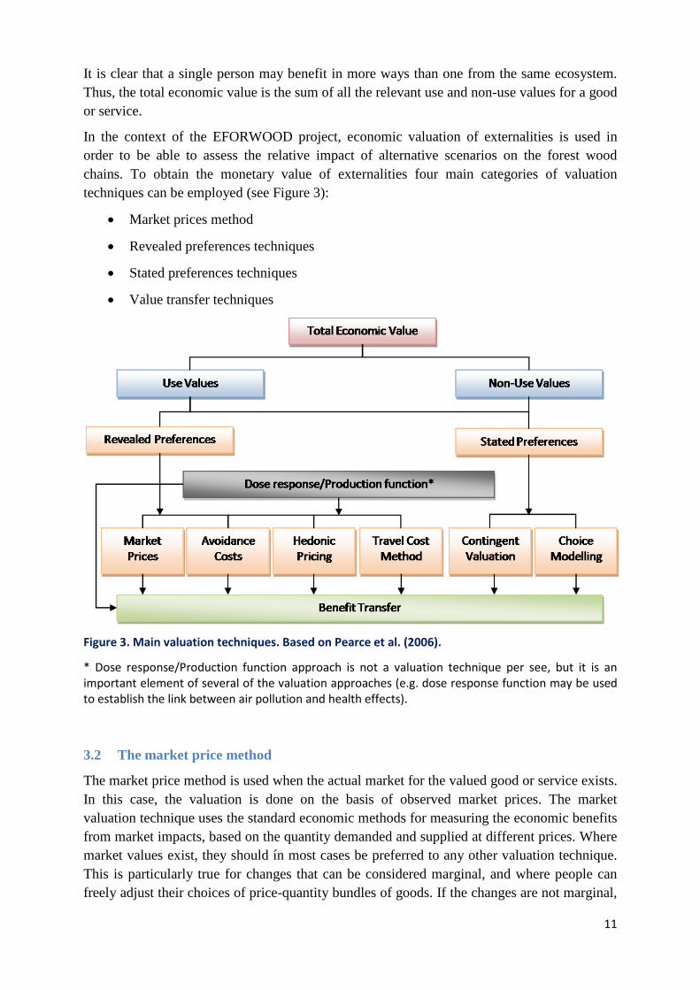
In the context of the EFORWOOD project, economic valuation of externalities is used in order to be able to assess the relative impact of alternative scenarios on the forest wood chains. To obtain the monetary value of externalities four main categories of valuation techniques can be employed (see Figure 3):
• Market prices method
• Revealed preferences techniques
• Stated preferences techniques
• Value transfer techniques
Figure 3. Main valuation techniques. Based on Pearce et al. (2006).
* Dose response/Production function approach is not a valuation technique per see, but it is an important element of several of the valuation approaches (e.g. dose response function may be used to establish the link between air pollution and health effects).
3.2 The market price method
The market price method is used when the actual market for the valued good or service exists. In this case, the valuation is done on the basis of observed market prices. The market valuation technique uses the standard economic methods for measuring the economic benefits from market impacts, based on the quantity demanded and supplied at different prices. Where market values exist, they should ín most cases be preferred to any other valuation technique. This is particularly true for changes that can be considered marginal, and where people can freely adjust their choices of price-quantity bundles of goods. If the changes are not marginal,

12
then the approach needs to take into account possible adjustments in prices and quantities in the market. It should be remembered, therefore, that market prices represent only a lower range estimate of value, as some people may be willing to pay more for the good than its price.
3.3 Revealed preferences techniques (RP)
When no direct market values exist for a good, it is sometimes possible to make some inference about their value from observations of expenditure on some other (related) market goods. Revealed preferences methods have been used extensively for the valuation of intangible goods like aesthetics or landscape views. Three basic valuation techniques exist:
• Avoidance cost method (also called replacement cost method)
• Travel cost method (TCM)
• Hedonic pricing method (HP)
Avoidance cost method is based on the idea that the cost incurred to avoid an effect or to replace the goods and services provided by an environmental resource can offer an estimate of the value for that resource. The main underlying assumptions for this approach refer to the predictability of the extent and nature of physical expected damage (there is an accurate damage function available) and that the costs to replace or restore damaged assets can be estimated within a reasonable degree of accuracy. It is further assumed that the replacement or restoration costs do not exceed the economic value of the service. The latter assumption, however, may not be valid in all cases. The value of the service may fall short of the replacement of restoration costs; either because there are few users or because their use of the service is in low-value activities. Therefore, the avoidance or replacement cost method is often only recommendable when several actual, implemented avoidance or replacement measures can be used to assess the cost. Otherwise, the exercise remains hypothetical and the assumption that values are likely to at least exceed costs has smaller credibility.
The travel cost method uses the costs of consuming the services of the environmental asset (e.g. outdoor recreation) as a proxy for value the consumers place on it. These costs include travel costs, entry fees, on-site expenditures and outlay on capital equipment necessary for consumption. This method requires surveys of visitors to provide information on travel expenditures (transportation mode, time and distance), socio-economic characteristics (age, gender, income, etc.) and purpose of the visit. In environmental economics, the travel cost method is mainly used to estimate economic use values associated with ecosystems or sites that are used for recreation (Hotelling, 1949; Freeman, 1992).
Hedonic pricing is used to estimate economic values for those goods and services that directly affect market prices of some other (related) goods or services. The basic premise of the hedonic pricing method is that the price of a marketed good is related to its characteristics, or the services it provides. For example, the price of a house reflects the characteristics of that house – size, age, comfort, location, air quality, etc. Therefore, it is possible to value the individual characteristics of a house or some other good by looking at how its price changes when the characteristics change. In environmental economics, the hedonic pricing method is most often used to value environmental amenities that affect the price of residential properties (Rosen, 1974), although it could also be used to estimate the value of the “green premium” on

13
environmentally friendly consumer goods, or the value of environmental risk on human health through wage differentials. In fact, labour economics is another field, where the hedonic method has received much empirical and theoretical attention (e.g. Ekeland et al 2004).
The main strength of the revealed preference techniques here is that they rely on people’s actual choices and behaviour. They also have challenges, for the travel cost method and in particular the hedonic method, issues of functional form, identification and simultaneity are technical issues with much research debate surrounding them. From an environmental economics point of view, they have however another short-coming and that is the fact that they cannot capture non-use values. By nature, non-use values are public goods that render exclusion impossible, and hence they are not embedded sufficiently in any particular marketed good or other consumption related activity. This is one reason for why the field of environmental economics has developed several stated preference techniques for environmental valuation.
3.4 Stated preferences techniques (SP)
The stated preference methods are based on hypothetical rather than actual data on behaviour; for the former the value is inferred from people’s responses to questions describing hypothetical markets or situations. They consist of the following main valuation techniques:
• Contingent valuation (CV)
• Choice modelling (CM)
The contingent valuation method assigns monetary values to environmental goods and services that do not involve market purchases and may not involve direct participation. It is carried out by directly asking individuals about their willingness-to-pay to obtain an environmental good or service. In the CVM, a careful description of the service involved is given to the individual, along with details about how it will be provided. The WTP value can be obtained in a number of ways, such as asking respondents to name a figure themselves (open-ended), either from multiple choice questions (payment card), or by asking them to say yes or no to a specific amount (in which case, follow-up questions with higher or lower amounts are often used – the referendum/dichotomous choice format). Contingent valuation can be used to estimate economic values for projects changing the supply of all kinds of ecosystem and environmental services (Mitchell and Carson, 1989).
Choice modelling is a newer approach to obtaining stated preferences. It consists of asking respondents to choose their preferred option from a set of alternatives, which are defined by attributes (including the price or payment). These alternatives are designed so that the respondents’ answer reveals the marginal rate of substitution7
7 Marginal Rate of Substitution is the rate at which a customer is ready to give up one good in exchange for another good while maintaining the same level of satisfaction.
between the attributes and money. These approaches are useful in cases when there is interest in the value of several attributes in a given situation or when the decision lends itself to respondents choosing from a set of alternatives described by attributes. Like contingent valuation, it can be applied to estimate the value of most goods and services (Henscher et al., 2005).

14
The methods have the strength of being fairly flexible and, theoretically, able to capture non-use values. Their main weakness is that the hypothetical nature of the set-up is believed to and has indeed been found to create a hypothetical bias. It may be possible, by various means, to reduce or assess this bias, but it is difficult (List et al 2006; Johansson-Stenman and Svedsäter, 2009).
3.5 Value transfer
Time and resources are often limited and new primary environmental valuation studies often cannot be performed prior to all important decisions. In search for more cost-efficient techniques, decision-makers are often forced to use the economic estimates of similar changes in environmental quality from previous studies to value the environmental change in question. Values from the original valuation study site can be transferred to the policy site in question. This procedure is most often termed benefit transfer, but could also be called transfer of damage or cost estimates. Hence, a more general term of value transfer (in line with Navrud and Ready, 2007) is used.
There are two main approaches to value transfer (Navrud, 2004), namely,
(i) Unit Value Transfer and
(ii) Function Transfer.
Unit value transfer (with or without adjustments) builds on the transfer of the actual value estimates from other studies, appropriately adjusted for inflation, differences in purchasing power of income across regions and in some cases also income variation. For example, where there are large differences in income levels between the study and the policy sites, the adjusted value estimate (e.g. willingness to pay) Vp at the policy site can be calculated as:
,
where is the original value estimate (e.g. willingness to pay) from the study site, and are the per capita income levels at the policy and study sites respectively, and β is the
income elasticity of willingness to pay for the environmental good in question8
In national value transfers, GDP per capita figures can be used as proxies for per capita income at the policy and study sites (Navrud, 2005). However, for international transfers this approach may give wrong results due to the differences in purchasing power parities (PPP)
(Pearce et al., 2006). The primary assumption in adjusting WTP values to a policy site is that the income elasticity of willingness to pay is one, however, as it has been noted that there is no reason to think that willingness to pay for environmental quality varies proportionally with income (Navrud, 2005). For example, Pearce (2003) reviewed the evidence on the income elasticity of WTP for environmental improvements and concluded based on the empirical estimates that the income elasticity of WTP for environmental change is less than unity, and that it probably lies in the range of 0.3-0.7.
8 The income elasticity of demand is given by the percentage change in quantity demanded (e.g. forest visits) divided by the percentage change in (per capita) income. The income elasticity of willingness to pay is measured by the percentage change in willingness to pay divided by the percentage change in income. The two concepts are essentially not the same. See Garrod and Willis (1999, 169-175).

15
between countries, therefore, it is recommended to use PPP adjusted GDP/capita for the international value transfers. This is the approach adopted in EFORWOOD as well (Annex II).
The Function transfer approach is more ambitious and suggests transferring instead value functions estimated in other studies – and not the actual values. Rather ‘local’ and case-relevant input (socio-demographic data etc) are used as input for the value functions to produce presumably better fitted value estimates for the case in hand.
Value transfer method has been the subject of considerable controversy, as it is often used inappropriately. The consensus seems to be that it can provide valid and reliable estimates under certain conditions. The conditions are: a) the commodity or the service being valued is very similar to the ones on which the estimates were made; b) the estimates – i.e. the site, the populations affected – must have very similar characteristics; c) the market conditions at both sites are similar; and d) the similar proposed changes in provision between sites. Of course, the original estimates being transferred must themselves be reliable in order for any attempt at transfer to be meaningful (e.g. Navrud and Brouwer, 2007; Bonnieux and Rainelli, 2003). If the conditions stated above are not adhered to, this can lead to bias or error and restrict the robustness of the benefit transfer process.
Some original estimates from the literature report values for an entire region, state or nation. Depending on the extent to which the criteria are satisfied and the degree of accuracy, there is some choice in the level of sophistication to be adopted for value transfer.
The value transfer is not without error. Bonnieux and Rainelli (2003) suggest that the average transfer error for spatial value transfers, both within and across countries, tends to be in the range of 25-40%, whereas individual transfers could have errors as high as 100-200%. In the validity studies, function transfer does not seem to perform better than unit value transfer. Therefore, it is usually recommended to use unit value transfer with the appropriate adjustments if necessary as the most transparent way of transfer – in spite of its apparent crudeness, and implied lack of attention to overall context variations.
Navrud and Brouwer (2007) identify the main steps for the value transfer:
1) Identify the change in the environmental good to be valued at policy site
a. Type of environmental good
b. Describe (expected) change in environmental quality
i. Baseline level
ii. Magnitude and direction of change (e.g. gain vs. loss, prevention vs. restoration)
2) Identify the affected population at the policy site
3) Conduct a literature review to identify relevant primary studies
4) Assess the relevance and quality of study site values for value transfer
a. Scientific soundness
b. Relevance

16
c. Richness in detail
5) Select and summarise the data available from the study site(s)
a. Define a lower and an upper bounds for the transferred estimates
b. Collect data on the mean estimate and standard error, and specific spatial transfer errors if available (if not, use the general transfer errors of +/- 25-40%)
6) Transfer value estimate from study site(s) to policy site
a. Determine the transfer unit
b. Determine the transfer method for spatial transfer
c. Determine the transfer method for temporal transfer
7) Assess uncertainty and acceptable transfer errors.
In the context of the EFORWOOD project, unit value transfer with adjustments has been adopted as a main valuation technique due to the fact that no funds were allocated to conduct primary valuation studies. The transfer unit (6a above) will depend on the actual externality valued (see Section 4). We undertake a spatial transfer adjustment for several externalities. For this we use variation in wealth and income (as captured in GDP/capita) also at the intra-national level, and for the international transfer, we used purchasing power parity corrected adjusted measures of these along with the related exchange rates (see Annex II). Across time, we apply assumptions on the growth in wealth and income (GDP/capita) and on the link between this measure and the valuation (see Annex I).
4 Obtaining values for specific externalities included in the EFORWOOD project
4.1 Recreation
4.1.1 Forest recreation in FWCs
The use of forest for recreation can have a significant value especially in densely populated countries. MCPFE (2007:240) defines forest recreation as “the use and enjoyment of a forest or wildland setting, including heritage landmarks, developed facilities, and other biophysical features”. Types of recreational activities refer to organised or free activities such as mushroom picking, hunting, fishing, mountain biking, walking, hiking, etc.
Recreation as a service is often not reflected by market prices (FAO, 2004; MCPFE, 2007; Zandersen and Tol, 2005). The economic value recreation brings could make a significant difference in the management, conservation and planning options for nature recreation. The forest management parts of the forest wood chain in the EFORWOOD project incorporate aspects of harvesting and other interrelated social and cultural values, including recreation. This allows us to identify and assess the possible impacts forest management alternatives may have on forest recreation in Europe. Within the forest wood chains, there are notable land management processes that with future scenario changes will have a direct impact on forest recreation; these include precommercial operations, harvesting, forwarding and skidding.

17
In a more indirect manner, recreation will also be affected by activities related to processing of wood as a raw material and the manufacture of wood based products. For example, in the advent of the A2 reference future (published by IPCC in 2000), where international timber imports will take precedence over European timber, there will be lower investments into forest management and a decrease in harvesting levels at a local level. This results in positive impacts on forest recreation, as land previously designated for harvesting will become areas for leisure pursuits.
In the context of the EFORWOOD project, currently there is no sufficient information at our disposal to make satisfactorily sound conjectures on the expected impact of scenarios under different reference futures for the analysed case studies. The available, albeit limited, information is regarding general description of reference futures. Information on process changes for recreation is based on EFORWOOD D.1.4.7 (2008) for a specific description of the forest wood chains (FWC).
On the level of the EU FWC, it is expected that under reference future A1, there will be a significant growth of tourism (on a general scale) in Atlantic and boreal Europe. Wilderness areas will be a major attraction from crowded and industrialised areas with high CO2 emissions and N-deposition. The increase in tourism will shift the focus of forest owners from timber production to facility management and visitor cash generation. As for reference future B2, the expectation is that although tourism grows, it would remain within Europe. Environmental tourism will be more localised and will become increasingly common. In all European regions, local tourism, biodiversity and wood production will be combined. Climate change will be limited, which will allow for new plantations of genetically improved tree species result in timber of higher density and better form. This will be especially noted in the Mediterranean region which will become an important wood production region. (EFORWOOD D.1.4.7, 2008)
4.1.2 Recreation in the indicator set in EFORWOOD
It is essential to understand the use of forests for recreation, since it will provide a gateway for understanding the value given to recreation in forests.
Most of the valuation studies on forest recreation report values on the size of the forest and the annual number of visits to recreation sites. Detailed information on forest characteristics, such as species composition, diversity and density of vegetation are often excluded, although these are believed to be important for the choice and length of recreation visits. The valuation studies based on the size of the forest are calculated in terms of willingness to pay per hectare (WTP/ha) (EXIOPOL, 2008; Zandersen and Tol, 2005). The size of the forest is thought to be able to capture the variation in the forest good valued.
The concept of capturing the value of recreation based on forest size is difficult for several reasons. Some WTP surveys ask for practices on a national scale, while others are based on local surveys - the data consequently reflects high non-use values when at a national level and higher resource conflicts when based at a local level.
Nearly all forests support recreational activities, the most intense visitor pressure comes from forests near urbanised areas or holiday centres. Access to a forest is a central issue to the trends in visitor numbers to forests. A small forested area may have a large recreational value

18
simply due to easy accessibility. For example, UNECE (2005) reports that 20% of visits takes place on 2% of forested land in Denmark; while in the Netherlands, 2 million visitors a year come to visit an forest of 2 000 ha. This means that the area of the forest is too crude a measure to capture people’s sense of scope of the value of the ecosystem.
This brings us to the second approach of using population characteristics, measured by the number of visits per year to a forest. Navrud and Brouwer (2007) show that WTP does not increase proportionally with the number of hectares, because recreation opportunities are found to be unaffected by the size of a forest, casting doubts on the use of values of forest recreation based on hectares. Additionally, Lindhjem and Navrud (2007) also state that they did not find any significant increase in WTP with the forest size, which could signify that the area of a forest is too crude a measure to capture people’s sense of scope for the WTP. They continue by suggesting that rather than focusing on WTP/ha, studies should focus on more important factors such as the characteristics of the population using the forest, the type of people, and the level of use on a geographical scale (local, regional, national). Socio-economic characteristics, such as income, have shown to vary considerably across studies. All change in the available capital a given population has to spend on recreation will have a marked impact on the WTP values for using a forest. This can be measured through the level of income of a given population.
Based on evidence from the empirical literature, WTP/ha was deemed to be unreliable (Navrud and Brouwer, 2007; Lindhjem and Navrud, 2007); therefore, in the facet of the EFORWOOD project, the CBA for forest recreation is based on WTP/visit and is linked to the indicator 16.2 - number of visits to forests per person per year.
4.1.3 Transfer of recreational values
In order to obtain the WTP/visit values for all the countries, the value transfer exercise based on the unit value transfer with income adjustment (a methodology described in Section 3.5) has been performed.
4.1.3.1 Selection of relevant studies
The list of selected studies used for benefit transfer of recreational use values is provided in Annex III.
The database includes 45 studies conducted from 1977 to 2008. Studies from the following countries are included in the database: Austria, Belgium, Czech Republic, Denmark, Netherlands, Finland, France, Germany, Hungary, Ireland, Italy, Norway, Poland, Spain, Sweden, and UK.
Studies were predominantly written in English, although some publications in German, French, and Spanish were also reviewed. All studies were peer-reviewed. The studies used face to face interviews, using entrance fees as the main payment vehicle. The data collected from the valuation studies includes information on:
(i) features and references of each study site;
(ii) types of recreational activities on site;
(iii) geographic location of the study region and study site;

19
(iv) entrance fees;
(v) number of visits per year; and
(vi) type of valuation methodology.
The information gathered from the literature represents the explanatory variables needed to compare sites across regions and countries – a necessary component to the value transfer approach (see Section 3.5). In addition, the selected studies have been filtered according to their scientific soundness, relevance for the value transfer exercise, and sufficient richness in detail.
The collected studies were identified in terms of methodology used for estimating the economic value of outdoor recreation. It is essential to understand how the estimates were calculated. The two main approaches used are revealed preference techniques (RP) and stated preference techniques (SP). Some authors test several model specifications for estimating recreational value using RP, such as the consumer surplus method (CS). RP are indirect methods that rely on the relationship between recreation participation and market-purchased goods necessary for recreation participation. SP are direct methods through which people express their willingness to pay (WTP) for environmental resources or recreation opportunities. SP results are given in WTP per person (or household) for a specifically defined unit (visit) or duration of time (day, year, several years, etc).
The most frequently used techniques in outdoor recreation economics to estimate the value of recreation are the contingent valuation method (CV) and the travel cost method (TCM). The CV method directly solicits information from people by asking them their maximum WTP or minimum compensation for a recreation experience. It also specifies the discrete changes in environmental quality (Mavsar, 2008). The TCM looks at how far visitors travel to come to a site. TCM is used to present results as the consumers’ surplus per activity day or per visit, and therefore represents the total willingness to pay net of cost for the forest recreation experience.
In principle, it is possible to combine the results of both RP and SP methods for value transfer, however, in EFORWOOD only the SP studies have been selected for value transfer in order to ensure the comparability of results across countries.
4.1.3.2 Harmonisation of values to €/visit per person per year
As it was mentioned in Section 4.1.2, the EFORWOOD indicator set provides basic data on the number of visits per person per year. It has to be mentioned that the number of visits does not necessarily reflect the actual length of time spent in the forests, or whether any time was actually spent in the forest as opposed to any additional facilities provided on site. This is a limitation that should be duly acknowledged. For the purpose of value transfer exercise, it was assumed that each visit lasts one day, that is, a payment per person per day was deemed equivalent to a payment per person per visit.
In cases where WTP values from the literature were given ‘per household’, further data was collected from national statistics accounts on the average size of households for each forest region. In cases where WTP values were given ‘per year’, it was assumed that forest sites in

20
or near urban areas were visited on average six times a year, and more remote forests were visited two to four times a year (see Table 3 for further information).
Table 3. Main assumptions for the harmonization of willingness to pay data.
Country Assumptions Source for average size per household
Austria • The size of a household is 2.56 people in 1994
Austrian Demographic Statistics
Denmark • The size of a household is 2.2 people in 1999 • Two visits are made per person per year
UNECE Statistic
Finland • The size of a household is 2.2 people in 1999 • Tax is paid once a year; and • Two visits are made per person per year
UNECE Statistics
Hungary • Two visits are made per person per year
Netherlands • The size of a household is 0.5 people in 1998
UNECE Statistics
Norway • The size of a household is 2.2 people in 2002 • Average of 4 visits per year per person for remote
forests, and 6 visits per person per year for urban forests
UNECE Statistics
Sweden • The size of a household is 2.6 people in 2005 Statistics Sweden
4.1.3.3 Spatial transfer of the values
In the course of recreational value transfer, two types of spatial value transfer have been identified:
(i) Within country value transfer
(ii) Across country value transfer
Within country value transfer have been applied in cases when a single set of recreational values (consisting of a minimum, a maximum and an average estimate) had to be produced for a country (or a specific region in that country) in which several primary valuation studies were identified. In such circumstances, additional data have been collected on the national and regional GDP per capita (for each region in which a primary valuation study have been conducted), and the unit value transfer have been performed using the GDP/capita as a proxy for the income adjustment.
For example, for a value transfer of recreational estimates to the case of Baden-Württemberg, the value transfer have been based on the GDP/capita of Baden-Württemberg and the GDP/capita of the regions in which original valuation studies have been conducted. The same method has been applied in order to obtain the recreational estimates for Västerbotten region in Sweden (present in the Scandinavian and Iberian chains).

21
Across country value transfer have been performed in for countries and regions where there was a lack of reliable primary valuation studies. In such case, the primary valuation studies from close by forests in neighbouring countries were used for the value transfer exercise, as geographical proximity of source and policy sites allows to minimize possible transfer errors (see e.g. Methodex D6, 2007).
The national figures for the GDP per capita9 were extracted from the World Bank World Development Indicator series (http://ddp-ext.worldbank.org), and the PPP adjusted GDP per capita values from EUROSTAT database (see Annex II).
All mean values were converted to Euro 2005 when necessary.
4.1.3.4 Time transfer of the values
When data was given for years other than 2005 (either prior or post 2005), the WTP estimates were updated to the year 2005 using the time update factor, calculated based on the constant GDP per capita country estimates from World Bank’s World Development Indicator series (http://ddp-ext.worldbank.org). The intertemporal elasticity for this time update is 1.0.
In order to account for the fact that willingness to pay for recreational use of forests may rise due to the increased income level, we introduce a concept of relative raising valuation. It basically means that WTP is assumed to grow with the GPD per capita growth. This assumption is incorporated in the analysis and allows for the WTP/visit values to obtained beyond the year 2005.
4.1.3.5 Income elasticity of WTP
Following from the unit transfer method described in Section3.5, in order to introduce and income adjustment of WTP values across regions (or countries), the income elasticity (represented by β) needs to be incorporated.
There is no consensus in the literature as to which is the appropriate income elasticity (Methodex D6, 2007) to adjust WTP values; consequently, we used a range of income elasticities (0.4, 0.5, 0.7, and 1.0). All the minimum values across all the income elasticity coefficients for all forest sites per country or per regional case study were averaged; similarly with all maximum values and all mean values of WTP per person per country. This gave a relative approximation for overall minimum, maximum and average value per visit to forests to be used in TOSIA.
4.1.3.6 Recreation values used in EFORWOOD
Table 4 presents the recreational values to be used for the CBA in EFORWOOD based on the value transfer exercise described in the preceding section.
9 World Development Indicator series reports GDP per capita at current and constant prices, of which the former ones were used in order to avoid inconsistencies with the regional GDP per capita values, extracted from national statistical sources and reported in current prices.

22
Table 4. Recreational values (willingness to pay per person per visit) for European countries and case studies, in €2005.10
Country
WTP in €/visit Low Medium High
Austria 0.7 2.3 6 Belgium 0.4 2.7 5.5
Bulgaria 0.2 3.1 6.4
Cyprus 1.4 5.7 10.3
Czech Republic 0.1 0.3 0.5
Denmark 1.1 4.8 10.5
Estonia 0.04 1.4 3.8
Finland 0.01 1.8 5.7
France 0.4 5.2 9.7
Germany 1.6 7 27
Greece 1.4 5.8 10.4
Hungary 0.6 4.2 7.5
Ireland 1.5 5.8 11.6
Italy 1.4 7.1 19.5
Latvia 0.6 1.9 3.3
Lithuania 0.7 2 3.5
Netherlands 1.5 3.1 5.8
Norway 0.9 3.8 9.2
Poland 0.6 1.2 1.75
Portugal 4.6 7.4 9.2
Romania 0.5 1.3 2.5
Slovak Republic 0.02 1.97 5.3
Slovenia 1.4 3.01 5.04
Spain 3.7 6.4 11.3
Sweden 0.02 1.02 3
United Kingdom 0.5 0.8 1.7
FWC Baden-Württemberg
1.8 8 30
FWC Scandinavia 0.5 1.2 1.9
FWC Iberia (Västerbotten)
0.01 4.1 11.5
FWC Iberia (France) 0.01 5.4 15.1
10 In what follows, €2005 refers to the values in EURO of the year 2005. Similarly, €2000 refers to the values in EURO of the year 2000.

23
4.1.3.7 Limitations of using value transfer for recreation
Navrud (2005) discusses several problems with applying value transfer for recreational benefits. First of all, the individuals at policy site may not value recreational activities the same as the average individual in the study site. This may be due to the fact that the individuals differ in terms of income (this can be corrected using adjusted value transfer), education or other socio-economic characteristics that affect their demand for recreation. In addition, even if the preferences of individuals were the same, the recreational opportunities (substitute sites or activities) are likely to be different.
An additional complication emerges when the willingness to pay values are reported on different terms. In most contingent valuation studies the results are reported for one or more specified discrete changes in environmental quality. In choice modelling methods or in some CV studies, however, the results are presented on marginal basis. If this is the case, the values can be directly comparable across countries. In case of discrete changes, the accuracy of the value transfer relies on several assumptions – the magnitude of the change, the initial levels of the environmental quality and the direction of change should be sufficiently similar at the study site and policy sites in order to minimize the transfer errors (Navrud, 2005).
4.2 Non-greenhouse gas emissions
4.2.1 Non-greenhouse gas emissions in FWCs
The valuation of air pollution (non-greenhouse gases) in the framework of EFORWOOD focuses mainly on carbon (CO), particulate matter (PM), nitrogen oxides (NOx), sulphur dioxide (SO2), and non-methane volatile organic compounds (NMVOCs) emissions. These pollutants cause health costs, damages to buildings and materials, crop losses and costs for further damages for the ecosystem (biosphere, soil, water). Health costs (mainly caused by PM from exhaust emissions or transformation of other pollutants) are considered to be by far the most important cost category.
In the context of the EFORWOOD project, currently there is no sufficient information at our disposal to make satisfactorily sound conjectures on the expected impact of scenarios under different reference futures for the analysed case studies. The available, albeit limited, information is regarding general description of reference futures. The general process is described in EFORWOOD D.1.4.7 (2008) for A1 and B2 reference futures and with more specific descriptions of the forest wood chains (FWC).
Expected impact of climate change IPCC scenarios on gas emissions
Overall, in B2, emissions continue to grow, albeit the growth of emissions is significantly slowed. In contrast, CO, NOx and NMVOCs emissions levels rise from the fossil fuel intensive reference future within A1, this results from the slowly declining population growth followed by an increasing agricultural productivity in A1.
On the level of the EU FWC, it is expected that under reference future A1, characterised on the one hand by a high economic growth requiring the use of a lot of energy, and on the other hand, the lack of environmental awareness, the fraction of bio-energy in total energy will stay the same as in 2005. Energy costs will be relatively low, resulting from the high prices combined with high economic growth, and there will be little pressure for more sustainable

24
and energy efficient homes. Impacts from air pollution will continue to affect health costs, from exhaust emission particles, corrosion from pollution will be more visible on buildings, ecosystems will further damaged by acid deposition, ozone exposition and SO2 (EFORWOOD D.1.4.7, 2008).
In contrast, in reference future B2 still within the level of the EU FWC, everybody will be able to afford bio-based power and high priority will be given to energy efficiency improvements and rapid development of renewable energy sources. An increasing share of bio-energy will be seen in households and consumption (EFORWOOD D.1.4.7, 2008).
On the level of the Baden-Württemberg FWC, it is expected that in the reference future A1, harvesting and hauling machines will use 20% bio-fuels and 80% fossil fuels. The same applies for the transportation processes. Consequently, non-GHGs still dominate the scene. In the reference future B2, bio-fuel consumption will increase considerably. Harvesting and hauling machines will use 40% bio fuels and 60% fossil fuels, resulting in a slight reduction of air pollution (EFORWOOD D.1.4.7, 2008).
4.2.2 Existing valuation studies
There are a considerable amount of studies on total, average and marginal costs of air pollution available. Within European studies the most commonly used research projects are: the Impact Pathway Approach (IPA) established within the ExternE (2005) project and CAFE CBA (AEA Technology, 2005). Other European projects such as HEATCO (2006) and IMPACT (2008) are also considered important. The impact pathway approach is regarded as the most advanced approach for the estimation of air pollution costs and is recommended by most experts as a best practice methodology.
Studies on air pollution costs cover in general the following impact categories:
• Health costs: impacts on human health due to the aspiration of fine particles (PMs and other air pollutants). Exhaust emission particles are considered the most important pollutant.
• Building and material damages: impacts on buildings and materials from air pollutants. Two effects are of importance: soiling of building surfaces/facades mainly through particles and dust; and degradation through corrosive processes due to acid air pollutants like NOx and SO2.
• Crop losses in agriculture and impacts on the biosphere: crops as well as forests and other ecosystems are damaged by acid deposition, ozone exposition and SO2.
• Impacts on biodiversity and ecosystems (soil and water/groundwater): the impacts on soil and groundwater are mainly caused by eutrophication and acidification due to the deposition of NOx.
The impact pathway approach looks at exposure-response functions from air pollution, the monetary valuation of impacts (for example ‘value of a statistical life’ based on willingness to pay) in the whole supply chain and the assessment of other indirect impacts like global warming, acidification and eutrophication. It follows the impact patterns on human health and the environment. It was developed by the ExternE Project series. The impact pathway approach quantifies impacts from airborne pollutants and looks at the chain of causal

25
relationships from pollution emission through transport and chemical conversion in the atmosphere, to the impacts on humans, crops, buildings or ecosystems. Welfare losses resulting from the damages incurred are transferred into monetary values. The impact pathway approach is commonly regarded as the preferred approach for environmental assessment as it allows for the estimation of site specific marginal external costs. The method has been used to support decisions concerning various air quality directives of the European Commission (e.g the ozone directive, national emissions ceiling directive, air quality guidelines on CO and benzene) (Friedrich and Bickel, 2001).
Impacts and damages are calculated using the following general relationships. The underlying form of the equation does not change, although it varies according to the different types of impacts. For example, functions which cause damage from acidic deposition take into account climate variables (such as relative humidity) and assess several pollutants simultaneously.
Impacts = Pollution x Stock at risk x Response function
Economic damage = Impact x Unit value of impact
Pollution is either expressed in terms of concentration or deposition. ‘Stock at risk’ is the amount of receptors (people, ecosystems, materials, etc.) present in the modelled domain.
A number of impact pathways must be implemented to generate overall benefits. For example, for the impact of ozone on crop yield, separate impacts on the different crops, each of which will differ in sensitivity is essential. For health impacts, the different effects must be quantified separately in order to understand the overall impact of air pollution on the population.
Its strengths include consistency and the consideration of different detailed input variables. However, the nature of it being a bottom-up approach makes it rather costly for deriving average and representative figures at national level (IMPACT 2008).
The Clean Air For Europe (CAFE CBA) (AEA Technology, 2005) programme performs a CBA of air pollution policies, by building on the policy assessments in RAINS integrated impact assessment model and the TREMOVE transport model. The RAINS model quantifies the costs for reaching health and environmental quality targets by identifying a cost-effective set of measures between alternative emission control strategies. The TREMOVE model is a policy assessment model, which assesses the effects of different transport and environment policies on transport emissions. The impacts are then assessed through the CAFE CBA (2005) model. The analysis of the costs effects takes place through the quantification of effects on health, crops, materials, social, and macroeconomic effects.
The following pollutants are treated within the CAFE CBA and are sorted according to their main impact category:
• Health (mortality, morbidity): PM, NO3, SO4 aerosols, SO2, VOCs, NO2. It is generally possible to quantify the impacts including their values. Uncertainties can be addressed using statistical methods and sensitivity analysis. Health impacts are believed to have the largest quantified monetary benefits with reduced air pollution. Their quantification deals both with mortality and morbidity, and as such CAFE CBA applies both the value of a statistical life (VSL) and the value of a life year (VOLY), as both approaches dispose of inherent uncertainty;

26
• Agriculture (crop yield, livestock): SO2, NOx, O3. The direct impacts of these pollutants are likely to be small in the CAFE CBA methodology, while indirect effects may be significant. This is mainly because increased air pollution could stimulate the performance of insects and other agricultural pests and diseases. The quantification process needs the estimated yield loss that is then multiplied by world prices as published by the FAO. World market prices are used as a proxy for shadow price, since these are closer to the real price of production, rather than being influenced by subsidies arising in local European prices;
• Materials (steel, concrete, building soil, paint, rubber): SO2, PM, O3. The quantification of material damage follows the work of the ExternE project. The impact pathway approach works well for those applications that are used in every day life. The same approach could in theory be applied to cultural and historic buildings. However, due to the lack of data the effects of air pollution on cultural heritage cannot be quantified. As a result, they are addressed qualitatively through an extended CBA framework; and
• Ecosystem (biodiversity, forest production): O3, N, SO2. The impacts are quantified relative to the risk measure. Risk measures can include the rate of deposition of acidifying pollutants relative to the critical load for acidification; an indicator of risks to biodiversity; and the rate of corrosion of building materials as an indicator of risks to historic monuments.
These effects are quantified to the extent possible using the impact pathway approach. The valuation is performed using the willingness to pay (WTP) approach in order to incorporate the receptors’ perspective. Some effects, such as damage to crops, buildings of little or no cultural merit, health costs, are done using suitable market research costs.
The ExternE (2005) project adopted the impact pathway approach for assessing the external impacts and costs resulting in the energy and transport use. ExternE (2005) measures the cost factors of air pollutants in terms of € per kg of pollutant emitted in the following impact categories:
• Health: PM10, SO2, NOx, O3. The damage costs of air pollution in ExternE (2005) are dominated by mortality. The key parameter in ExternE (2005) is the value of statistical life (VSL), i.e. the collective willingness to pay for reducing the risk of premature death. Values were derived from three surveys undertaken simultaneously in the UK, France and Italy. In 1998, ExternE set the Europe-wide value for VSL of €3,1million, which was close to similar studies in the USA. ExternE (2005) bases the valuation on Years of Life Lost (YOLL) rather than multiplying the number of premature deaths by VSL. The YOLL value from air pollution is €0,083 million/year.
• Cultural and historical heritage: PM10, SO2, NO3. Few quantification efforts have been made regarding the acidification impacts on buildings. This is thought to be due to the level of uncertainty in the quantification process and the lack of an inventory on European stock at risk. Furthermore, maintenance costs are likely to vary according to the historical building. Aesthetic loss is subject to individual perception and would need a specific study; e.g. a contingent valuation study.

27
• Visibility: NOx and PM. Visibility relates to the reduction of visual range resulting from the presence of air pollutants in the atmosphere. This is a relatively new approach for Europe, and thus, the issue has received little attention. The only known European valuation studies are those from ExternE. Air pollution policy or regulation studies can be used to estimate a general relationship between the level of improvement in visibility and the average household WTP on such an improvement.
• Crop loss: Up-to-date prices of cropes per tonne are provided by FAOSTAT and IFS.
It must be noted that secondary pollutants are the result of primary pollutants emitted into the atmosphere and undergo a transformation that causes harmful impacts in their latter form. For example, SO2 (primary pollutant) is transformed into sulphate aerosols (secondary pollutant), and similarly NOx into nitrate aerosols. The impact of secondary pollutants take some time as it occurs over distances of tens to hundreds of km. The damage from primary pollutant depends on local conditions, where it is deposited and becomes reactive. The costs, however, should be accounted for at the emission site. Particles emitted by cars are PM2.5 (N.B. PMx.x designates particles with diameter less than x.x microns) and are especially harmful because they penetrate deep into the lungs (IMPACT, 2008).
HEATCO (2006), on the other hand, measured the cost factors of pollutants in terms of € per tonne of pollutant emitted in different environments (urban areas, outside built-up areas). Their list of pollutant covers:
• PM2.5 for transport emissions (PM10 for emissions from power plants);
• NOx as precursor of nitrate aerosols and ozone;
• SO2 for direct effects and as precursor of sulphate aerosols; and
• NMVOCs as precursors of ozone.
HEATCO (2006) is also of the opinion that human health costs are the most important effects in terms of quantifiable costs. They use YOLL as an indicator for physical impacts that contribute to health costs. In addition, the monetary values given to each pollutant emitted as well as YOLL include a number of other health impacts and in addition damage to crops and materials (for further information see Table 0.11 p.S19, HEATCO, 2006).
The variation in costs due to NOx, NMVOCs and SO2 between countries is mainly caused by air chemistry (including ozone formation) and the population affected. For PM, no air chemistry is involved, and thus, the impacts are determined mainly by distance of the population to the emission source and the prevailing wind direction. NOx, NMVOCs and SO2 have virtually no local effects as most of their impacts are caused after chemical transformation to secondary pollutants (ammonium nitrates and sulphates, ozone). Damages occur far from the emission source, mostly in other countries. Trans-boundary impacts are valued at European averaged values.
HEATCO (2006) recommend that the increasing values for future years are based on a default inter-temporal elasticity to GDP per capita growth of 1. For sensitivity analysis, they recommend testing using 0.7 for income elasticity to see if air pollution costs prove to contribute an important part of the benefits quantified.

28
Air pollution costs in IMPACT (2008) are caused by the emission of air pollutants such as PM, NOx, SO2 and VOCs and consist of health costs, building/material damages, crop losses and costs for further damages to the ecosystem (soil, water, biosphere). Health costs (mainly from PM, from exhaust emissions or transformation of other pollutants) are by far the most important cost category. The costs of some pollutants are greater than those for other pollutants; however, this is mainly based on estimations carried out by the ExternE (2005) model. The air pollutants dealt within IMPACT (2008) in the following categories include:
• Health costs: PM2.5, PM10, O3;
• Building and material damages: NOx, SO2;
• Crop losses in agriculture and impacts on the biosphere: SO2; and
• Impacts on biodiversity and ecosystems (soil and water/groundwater): VOCs.
4.2.3 Comparison of valuation studies
From the described studies, there are similarities between ExternE (2005), HEATCO (2006) and CAFE CBA (AEA Technology, 2005) models. Within CAFE CBA basic values for VOLY and VSL, are based on the same source (NewExt, 2005) as HEATCO and ExternE. Additionally, CAFE CBA presents the ranges of results by taking into account different valuation methods for VOLY and VSL (use of median and mean estimates). Similarly to HEATCO, the CAFE CBA and the ExternE also take into account material and building damages.
The most important figures produced by the CAFE CBA (AEA Technology, 2005) for all EU countries were the costs for PM2.5 and for NOx. The values per tonne for PM2.5 vary between €8 600 -25 000 (low/high values for Greece) and €63 000 -180 000 (low/high value for the Netherlands). The values per tonne of NOx are for most countries considerably lower (IMPACT, 2008).
The ranges of damage costs in HEATCO (2006) and CAFE CBA (AEA Technology, 2005) are similar in magnitude, but there are some important differences with respect to different aspects (cost categories covered, toxicity of different pollutants, especially primary and secondary PM2.5 and PM10, inclusion of local damages, valuation factors for mortality and morbidity).
Differences between the HEATCO (2006) and CAFE CBA (AEA Technology, 2005) studies are as such (IMPACT, 2008; ExternE, 2005):
• Crop losses and material damages: CAFE CBA values only cover health costs and ozone caused crop losses. However, with respect to total costs the exclusion of material damages in CAFE CBA has only minor effects;
• Toxicity of PM2.5/PM10 from different sources: Whereas HEATCO and ExternE treat secondary particles (nitrates and sulphates) differently than primary exhaust emissions, based on the review from WHO (cited in AEA Technology, 2005), CAFE CBA argues that there is less scientific evidence to establish different risk rates fro different kind of particles.

29
• Inclusion of local effects: CAFE CBA does not take into account local effects of PM2.5 emissions, while HEATCO and ExternE does, in terms of human health between urban and interurban traffic situations.
• Health valuation: there is a wider range of results of CAFE CBA compared to HEATCO and ExternE. The HEATCO results correspond to the median VOLY results of CAFE CBA. In addition, it has to be considered that ExternE and HEATCO uses a factor cost approach, whereas CAFE CBA valuation is based on market prices.
• CAFE CBA does not take physical or chemical characteristics into account and as such assumes that all particles are equally aggressive per unit mass. There is a lack of quantitative base from which to establish different risk rates for different particles. As a result, experts working on the WHO review CAFE CBA have declined to take a position on the differences in risk between particles per unit mass.
• HEATCO uses the ExternE (2005) methodology, which underlines the high particles and especially particles from internal combustion engines. They state that there is a lack of evidence for harmful effects in secondary particles of nitrates, while the contrary is true for sulphates where the harmful associations have been clearly demonstrated. Therefore, different particle fractions and sources are treated differently.
Each approach has its own advantage. Whereas HEATCO (2006) provides differentiated values for different types of networks and regions especially regarding PM2.5/PM10, CAFE CBA (AEA Technology, 2005) provides for other pollutants results on the basis of a peer reviewed project, thought to be robust. With respect to the valuation of secondary particles (nitrates, sulphates) CAFE CBA is more cautious and values these particles equally as primary exhaust particles.
IMPACT (2008) recommends the use of a combined approach between using HEATCO results for the valuation of PM2.5/PM10 emissions and the CAFE CBA results for the valuation of emissions of other pollutants.
4.2.4 Monetary values used in EFORWOOD
The monetary estimates of non-greenhouse gas emissions for the use within the EFORWOOD project presented in Table 5 are given in €/kg for each subcategory and are differentiated by country. The estimates are based on a review of European valuation studies (see Section 4.2.2) following the recommendations of IMPACT (2008) and EEA (2000).

30
Table 5. Pollution costs in €2005/kg of pollutant.
Country NOx NMVOCs CO
SO2 L M H L M H L M H Austria 1.18 4.69 9.10 0.0533 0.92 1.78 0.00829 0.01633 0.02438 8.68 Belgium 0.71 2.82 5.47 0.0789 1.35 2.63 0.00826 0.01627 0.02429 1.16 Bulgaria 0.32 1.25 2.42 0.0081 0.14 0.27 0.00945 0.01863 0.02781 1.35 Cyprus 0.07 0.28 0.54 0.0097 0.17 0.32 0.00860 0.01695 0.02530 2.15 Czech Republic 1.15 4.55 8.83 0.0363 0.62 1.21 0.00943 0.01859 0.02775 9.67 Denmark 0.60 2.39 4.64 0.0221 0.38 0.74 0.00829 0.01633 0.02438 5.48 Estonia 0.16 0.62 1.21 0.0045 0.08 0.15 0.01506 0.02967 0.04428 2.72 Finland 0.12 0.46 0.89 0.0067 0.12 0.22 0.00981 0.01933 0.02885 2.01 France 1.05 4.16 8.08 0.0441 0.76 1.47 0.00819 0.01614 0.02409 8.39 Germany 1.28 5.09 9.88 0.0525 0.90 1.75 0.00781 0.01539 0.02297 11.32 Greece 0.13 0.50 0.97 0.0109 0.19 0.36 0.00966 0.01904 0.02842 1.70 Hungary 0.88 3.48 6.75 0.0338 0.58 1.13 0.01064 0.02097 0.03130 6.00 Ireland 0.58 2.31 4.48 0.0248 0.42 0.83 0.01310 0.02582 0.03854 5.66 Italy 0.75 2.95 5.73 0.0332 0.57 1.11 0.00771 0.01520 0.02269 6.13 Latvia 0.28 1.10 2.14 0.0092 0.16 0.31 0.01457 0.02870 0.04284 3.06 Lithuania 0.35 1.38 2.69 0.0090 0.15 0.30 0.01346 0.02652 0.03959 3.58 Netherlands 0.89 3.51 6.82 0.0589 1.01 1.96 0.00854 0.01682 0.02511 13.44 Norway 0.28 1.12 2.17 0.0098 0.17 0.33 0.00888 0.01750 0.02612 2.71 Poland 0.60 2.36 4.58 0.0211 0.36 0.70 0.01114 0.02196 0.03277 6.57 Portugal 0.17 0.67 1.31 0.0151 0.26 0.50 0.00853 0.01681 0.02509 3.52 Romania 0.39 1.55 3.01 0.0000 0.27 0.55 0.00947 0.01866 0.02786 2.74 Slovak Republic 0.85 3.35 6.51 0.0263 0.45 0.88 0.00065 0.00128 0.00192 6.13 Slovenia 1.04 4.10 7.96 0.0499 0.86 1.66 0.01034 0.02038 0.03042 7.37 Spain 0.37 1.60 2.83 0.0131 0.22 0.44 0.00907 0.01788 0.02668 4.68 Sweden 0.32 1.25 2.43 0.0099 0.17 0.33 0.00905 0.01784 0.02663 3.09 United Kingdom 0.56 2.22 4.30 0.0364 0.63 1.21 0.00888 0.01750 0.02613 7.29 Source: derived from AEA Technology (2005); except that CO values are derived from Rabl and Spadaro, 2000 Notes: For CO, NOx and NMVOCs, low values (L) represent vehicle types ranging between 1.4litres < CC <2.0 litres; medium values (M) represent the mean between the low and high values; and high values (H) represent values given by AEA Technology (2005). The high values provided are not the highest possible value, they are only estimated values derived from the 8 AEA Technology (2005)
Values for NOx, NMVOCs and SO2 were based on the CAFE CBA (AEA Technology, 2005) (see Table 6) and those for CO were based on the value from Rabl and Spadaro (2000) (i.e. 0.02 in €1994/kg of CO for France). These were then updated to the year 2005 using the time correction factors listed in Annex II.

31
Table 6. Pollution costs used in CAFE CBA (AEA technology, 2005) in €2000/ton of pollutant.
Countries NOx NMVOC SO2
Austria 8700 1700 8300 Belgium 5200 2500 1100 Bulgaria 1800 200 1000 Cyprus 500 300 2000 Czech Republic 7300 1000 8000 Denmark 4400 700 5200 Estonia 800 100 1800 Finland 800 200 1800 France 7700 1400 8000 Germany 9600 1700 11000 Greece 800 300 1400 Hungary 5400 900 4800 Ireland 3800 700 4800 Italy 5700 1100 6100 Latvia 1400 200 2000 Lithuania 1800 200 2400 Netherlands 6600 1900 13000 Norway 2000 300 2500 Poland 3900 600 5600 Portugal 1300 500 3500 Romania 2200 400 2000 Slovak Republic 5200 700 4900 Slovenia 6700 1400 6200 Spain 2600 400 4300 Sweden 2200 300 2800 United Kingdom 3900 1100 6600 Source: AEA Technology, 2005 Note: Values for NOx, SO2 and NMVOCs are based on the value of a life year (VOLY) median
For most countries there is a lack of data on emission rates and values. In order to estimate the range of low, medium and high values for ToSIA, the EEA (2000) methodology was used to calculate the lower bound values of emissions in Europe. The EEA developed an approach for the different types of vehicle categories and types of emissions, according to the availability of input data available; this approach was then accommodated to fit the needs of the EFORWOOD project. In the case of EFORWOOD, the main vehicle categories of interest are those for LDVs and HDVs. Assumptions of the EEA methodology for any pollutant is to use the rate of emission reduction factor of the vehicle class (in this case LDVs or HDVs) as the ratio of the respective emission standard. A reduction factor is employed since vehicle emissions are based on ‘cold’ emissions (i.e. the warming-up phase) and ‘hot’ emissions fractions (i.e. the thermal stabilised engine operation). Their representative reduction factors for the lower bound levels of emissions are given in Table 7 for pollutants CO, NOx, and NMVOCs. The calculations are done using the following equation:

32
kEuroijikji ERFE ,,,,, *100/)100( −=
where,
i = pollutant i ;
j = vehicles class j
RF= reduction factor
K= type of roads
Euro = emission values in €/kg (as shown in Table 6).
Table 7. Summary of the emission reduction factors.
Emission reduction factors for vehicle class 1.4 l < CC < 2 l CO emission factor (%) CO (%) 66 NOx (%) 87 VOC (%) 97 Source: Adapted from Table 5.6 in EEA (2000). Note: Following recommendations from EEA, VOC values are applied to calculate the over-emissions of both NMVOCs and CH4 during cold start.
It must be noted that the EEA (2000) found it difficult to quantify changes in the percentage of methane in the total NMVOCs fraction due to a lack of available data. The actual fact is that there is an increase in emissions of methane for late catalyst vehicles due to the slower oxidation in the catalytic converter, compared to larger molecule hydrocarbons. Therefore, the methodology assumes that there no percentage increase in methane for the vehicle emission reduction factor of the NMVOCs.
4.3 GHG emissions and carbon stock in FWCs
Forests have an important role to play in the mitigation of greenhouse gas emissions. Plants absorb carbon in the form of carbon dioxide (CO2) from the atmosphere. Trees in forest can continually sequester carbon over the course of years to centuries; thus making forests a very effective land use type for withdrawing large amounts of carbon from the atmosphere over long periods, if the forest ecosystem is not disturbed by natural of human-induced processes, such as forest fires or harvesting activities.
The most direct impacts are related to the different forest management strategies, since these are responsible for the treatment of forest stands from an ecological and an economic perspective. Forest management strategies include those: (i) for conservation, where the role of forests is to conserve existing carbon pools in the forests and thus prevent emissions in the atmosphere by restricting harvesting activities, rotation lengths or thinning intensity; (ii) for storage, by increasing the forest area in order to increase the capacity of carbon storage in the forest; (iii) for wood production, where there is a transfer of wood biomass into products (e.g. construction, furnishing, biofuel). For the purpose of this study, carbon stocks refer to carbon in:
• Living woody biomass above ground;
• Living woody biomass below ground;

33
• Dead wood;
• Soils of forest; and
• Wood products.
Further impacts are found in the chain of custody, referring to the use and processing of the harvested wood. These impacts may be related to the further use and processing of wood and wood products, and also include emissions from machinery and wood combustion. After harvesting, forest products continue to store carbon for a certain time. Thus, forests can provide both a store of carbon as well as new raw material. Only with decay of the forest products (litter, organic material in the soil, wood-based products) will the carbon be released back into the atmosphere. However, as this topic is relatively new there are still great uncertainties in the particular lifespan of wood taken from forests and the level of emissions from the various greenhouse gases. Value estimates in this study are calculated for carbon dioxide (CO2) and carbon (C)11
4.3.1 Changes in the GHG emissions and carbon stock processes
.
In the context of the EFORWOOD project, currently there is no sufficient information at our disposal to make satisfactorily sound conjectures on the expected impact of scenarios under different reference futures for the analysed case studies. The available, albeit limited, information is regarding general description of reference futures. The general process is briefly described in Lousteau (2001) for A1 and B2 reference futures, and in as well as in EFORWOOD D.1.4.7 (2008) for a specific description of the forest wood chains (FWC).
Overall, carbon stock changes in the A1 cover are predominately related to land use change from loss of forest cover. In the B2 reference future, carbon stocks continue to grow and provide the highest sequestration rates, albeit that in the long run the accumulation rate is significantly slowed. Differences are found in the spatial distribution of sinks and sources between the scenarios, illustrating that land use is an important factor in future carbon sequestration changes that cannot be ignored. Given the higher temperatures, particularly in summer, and more winter precipitation along coasts (except for the Mediterranean) and in mountain ranges (except for the Pyrenees), there is likely to be a shift in the forest types under B2 as soil water supply is sharply reduced for the vegetation (Lousteau, 2001). Water storage capacity of soils in forest areas and local conditions in terms of nutrient supply will be key factors in governing carbon sequestration.
CO2 emissions related to land-use change in the A1 cover the widest range of energy related emissions. CO2 emissions from loss of forest cover are said to peak after several decades, and then gradually decline. The eventual stabilisation results from an accumulation of CO2 emissions, than by the way emissions change in that period (IPCC, 2000). In EFORWOOD, land-use changes as such, and the implied effects on CO2 emissions are not explicitly included and modelled.
11 Note that in literature the costs of carbon dioxide are expressed in monetary units per tonne of carbon (C) or per ton of carbon dioxide (CO2). Costs per ton of C translate into costs per ton of CO2 by dividing by a factor 44/12 = 3.667, reflecting the molar weight ratio of CO2 to C.

34
On the level of the EU FWC, it is expected that under reference future A1, traditional manufacturing will be moved out of the European region, and in areas of lower labour and transport costs (e.g. Russia, Africa). The free trade of goods, and cheap raw materials being imported from outside Europe, will result in less harvesting from European forests. Since agriculture will be out-competed in a free trade world, land abandonment takes place at a large scale throughout Europe. Often, these abandoned lands are planted with trees and converted to forest. As a result, carbon stock is expected to increase on the long haul (EFORWOOD D.1.4.7, 2008).
In contrast, demand for hardwood in Europe will do relatively well because specific high quality assortments will be very expensive (wealthy urbanised societies like exclusive wooden furniture) and because resources of tropical hardwood will be getting depleted. Harvesting of hardwoods will be based on clear felling regimes with single coupes being large and intense (EFORWOOD D.1.4.7, 2008).
Forest management will take place in regions where production is competitive with imported material. Growing stock in these regions will increase overall, leading to old forests, with more natural dynamics and carbon sequestration (EFORWOOD D.1.4.7, 2008).
In contrast, in reference future B2, climate change is limited, reducing GHG emissions. Furthermore, the Mediterranean becomes an important wood production region (EFORWOOD D.1.4.7, 2008).
On the level of the Baden-Württemberg FWC, it is expected that in the reference future A1, there will be no changes in silvicultural management, or in terms of volume of wood produced. The source of timber for bio-energy will come from plantations, basically agricultural land which will be switched to short-rotation plantations and biomass crops. Harvesting and hauling machines will use 20% bio fuels and 80% fossil fuels. The same shares will apply for the transportation processes (EFORWOOD D.1.4.7, 2008).
In the reference future B2, bio-fuel consumption will increase considerably. Harvesting and hauling machines will use 40% bio fuels and 60% fossil fuels. The same shares will apply for the transportation processes (EFORWOOD D.1.4.7, 2008).
On the level of the Scandinavian FWC, changes in carbon stock will be noted as there will be an increase in demand for wood as a raw material. The increase in bio-energy will also encourage new types of harvesting, reducing the need for clear felled land (EFORWOOD D.1.4.7, 2008).
4.3.2 Methods to estimate the price of carbon dioxide emissions
There are various methods to price carbon dioxide emissions:
• marginal damage cost of carbon dioxide emissions
• marginal abatement cost of carbon dioxide emissions
• spot and future prices in ETS markets
We briefly discuss these methods.

35
4.3.2.1 The marginal damage cost method
The marginal damage cost of CO2 is the welfare loss due to a small increase in emissions. It is also called the social cost of carbon. From the perspective of economic theory, this is the so-called Pigouvian tax on CO2 and it represents the net present value of the damage done by an infinitesimally small increase in emissions along the optimal emission trajectory.
The damage cost approach uses detailed modelling to assess the physical impacts of climate change and combines these with estimations of the economic impacts resulting from these physical impacts. The estimation of economic value of non-market impacts calls for the use of non-market valuation techniques, which were briefly introduced in Section 3. The economic valuation in the area of climate change, however, is rather controversial. Firstly, there is a general lack of knowledge about the physical impacts caused by global warming. While some impacts can be modelled with a certain precision, some other impacts are often “ignored”, because the knowledge on the links between global warming and these impacts are known (e.g. extended flooding, slow-down of the Gulfstream). Secondary impacts, such as socially contingent damages (e.g. regional conflicts) are even more difficult to assess. Estimates of the future emissions and climate change add another layer of uncertainty.
Available damage cost estimations of GHG emissions vary greatly depending on the valuation method used and the underlying assumptions on the discount rate, the approach used to weighting impacts in different regions and on the time horizon (Tol, 2005). A recent detailed assessment of damage costs was carried out by the Social Cost of Carbon project (http://socialcostofcarbon.aeat.com/index.htm) conducted by AEA Technology and the Stockholm Environmental Institute on behalf of Defra, UK (SEI, 2005). The study reviewed a large number of existing estimates of damage cost and compares them to own modelling results. Some of the results are presented in Table 8 below.
Table 8. Example of the evolution of damage costs of CO2 over time (PAGE results for social cost of carbon value). Values presented in £/tC for year of emission.
Year 5% Mean 95% 2001 9 46 130 2010 12 61 159 2020 14 77 215 2040 27 127 324 2060 34 187 513 Source: adapted from SEI, 2005 (in Watkiss, 2005) Notes: Based on the A2 scenarios, with PPP exchange rates, Green book social rate of time preferences, an equity weight parameter of 1. The PAGE model results include some (but not all) major climatic system events but exclude any socially contingent effect.
A summary of some of the most important studies estimating the damage costs of climate change is given in Table 9 below (extracted from the IMPACT, 2008).

36
Table 9. Overview of the damage costs of climate change as estimated by various studies (in €/tCO2).
Source Year of application
Min Average
Max Comments
ExternE, 2005
2010 9
Watkiss, 2005 2000 2010 2020 2030 2040 2050
14 17 20 25 28 36
22 27 32 39 44 57
87 107 138 144 162 198
Results based on damage costs only
Watkiss, 2005 2000 2010 2020 2030 2040 2050
14 16 20 26 36 51
22 26 32 40 55 83
51 63 81 103 131 166
Results based on comparison of damage and avoidance costs
Tol, 2005 -4 11 53 Based on studies with PRTP = 1% Stern, 2006 2050
2050 2050
71 25 21
Business as usual scenario Stabilisation at 550ppm Stabilisation at 450ppm
DLR, 2006 15 70 280 Based on Downing 2005 Source: IMPACT (2008)
The IMPACT report (IMPACT, 2008) summarizes the critical aspects determining uncertainties in valuation studies based on damage costs:
• Assessment of the worldwide long term economic development, technological developments, the associated greenhouse gas emissions for the baseline scenario compared to which the marginal external costs of additional CO2 emissions are to be assessed.
• Assessment of the physical impacts of climate change and selection of the impacts included in the analysis.
• Assessment of the economic impacts resulting from the estimated physical impacts and selection of the impacts valued in the analysis.
• The discount rate used.
• Consideration of major risks and dramatic changes of the climate (e.g. slowing down of the golf stream).
• The approach to weighting impacts in different regions (called equity weighting).
• The time horizon used.

37
4.3.2.2 The marginal avoidance cost method
An alternative method which avoids the uncertainties associated with assessing damage costs of climate control is to assess the costs of avoiding CO2 emissions. This method is referred to as avoidance cost, abatement cost or mitigation cost method. This approach has been applied and recommended in several studies (e.g. UNITE, 2001; and ExternE, 2005).
The method is based on a cost-effectiveness analysis that determines the least-cost option to achieve a required level of GHG emission reduction, e.g. related to a policy target. The costs of reaching a certain target are calculated using a cost curve approach or other methodologies. The target can be specified at different system levels, e.g. at a national, EU or worldwide level, and may even be defined on a sector level. For CO2 emissions, the targets are usually based on the ones set out by Kyoto Protocol.
An overview of some of the most important studies estimating the avoidance costs of climate change is given in Table 10 below.
Table 10. Overview of the CO2 avoidance costs (in €/kg of CO2) as estimated in selected studies.
Source Avoidance costs (€/kg CO2) Year Low Med High Reference for avoidance costs
RECORDIT, 2000 and 2001
2010 0.037 Kyoto target Long term IPPC 50% reduction target 2050 0.135
Capros and Mantzos, 2000
2010 0.005 0.038 Kyoto target: lower value based on trading with countries outside the Eu, upper value on situation without trading outside the EU
UNITE, 2001 2010 0.005 0.02 0.038 Based on Capros and Mantzos, 2000 INFRAS, 2004 2010 0.02 Kyoto target Long term IPPC 50% reduction target
2050 0.14 ExternE, 2005 2010 0.005 0.019 0.02 Kyoto target Long term IPPC 50% reduction target
2050 0.095 Stern, 2006 2015 0.032 0.049 0.065 Average abatement cost
2025 0.016 0.027 0.045 2050 -0.041 0.018 0.081
SEC, 2007 8 2010 0.013 Stabilisation at 2ºC temperature increase. Linear extrapolation based on 2020-2030 data 2020 0.048
2030 0.064 2050 0.120
Source: adapted from IMPACT (2008)
The IMPACT report (IMPACT, 2008) summarizes the critical aspects determining the accuracy of avoidance cost estimates:
• The choice of the target level that is used to assess avoidance costs, with regard to the:
• System to which the target is applied (e.g. all sectors vs. specifically for a certain sector or a country/region vs. worldwide).
• The numerical value of the target level, based on scientific evidence.

38
• Political and public acceptance; formally only legally binding targets laid down in national law or international agreements can be considered as a valid indication of the (society’s) willingness to pay.
• Time horizon (short term versus long term).
• Estimation of the greenhouse gas reduction potential of technical and non-technical options.
• Assessment of the future costs of technical and non-technical options in various sectors to reduce greenhouse gas emissions.
• Assumptions on the energy costs used in the assessment of avoidance costs for the technical and non-technical options
• As explained in Section 3.3, a challenge for the avoidance cost method is that it should rely preferably on actual actions and measures taken, to have reasonable credibility as a substitute for a true welfare change measure. As climate change and mitigation policies are still very much in their making and infancy, this limits the potential of the avoidance cost method.
4.3.2.3 Market-based pricing methods
Another option to price carbon dioxide emissions is to use the information revealed by markets, which aggregates the preferences of a large number of firms with a strong interest in accurate pricing.
A market for carbon emissions has been created with the establishment of the European Trading Scheme (ETS). The EU-ETS began trading on January 1, 2005. The prices have been very volatile – ranging from almost 30€/tCO2 to almost 0€/tCO2 (see Figure 4). This pronounced volatility is apparently due to a market perception that the permit allowances were excessively generous relative to expected emissions.
Figure 4. Spot price of carbon dioxide emission allowances in the ETS. Source: http://www.eex.com/en/Download/Market%20Data.
0,00 €
5,00 €
10,00 €
15,00 €
20,00 €
25,00 €
30,00 €
25/1
0/20
04
25/1
1/20
04
25/1
2/20
04
25/0
1/20
05
25/0
2/20
05
25/0
3/20
05
25/0
4/20
05
25/0
5/20
05
25/0
6/20
05
25/0
7/20
05
25/0
8/20
05
25/0
9/20
05
25/1
0/20
05
25/1
1/20
05
25/1
2/20
05
25/0
1/20
06
25/0
2/20
06
25/0
3/20
06
25/0
4/20
06
25/0
5/20
06
25/0
6/20
06
25/0
7/20
06
25/0
8/20
06
25/0
9/20
06
25/1
0/20
06
25/1
1/20
06
25/1
2/20
06
25/0
1/20
07
25/0
2/20
07
25/0
3/20
07
25/0
4/20
07
25/0
5/20
07
25/0
6/20
07
25/0
7/20
07
25/0
8/20
07
25/0
9/20
07
25/1
0/20
07
25/1
1/20
07
25/1
2/20
07
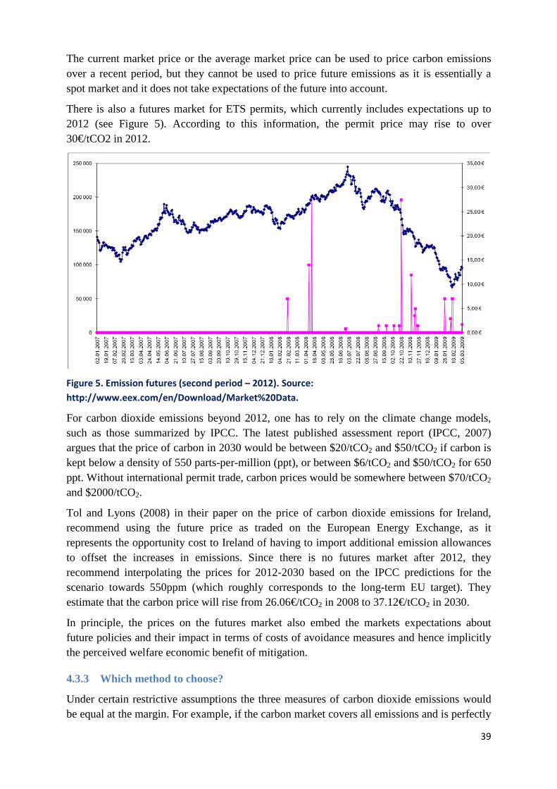
39
The current market price or the average market price can be used to price carbon emissions over a recent period, but they cannot be used to price future emissions as it is essentially a spot market and it does not take expectations of the future into account.
There is also a futures market for ETS permits, which currently includes expectations up to 2012 (see Figure 5). According to this information, the permit price may rise to over 30€/tCO2 in 2012.
Figure 5. Emission futures (second period – 2012). Source: http://www.eex.com/en/Download/Market%20Data.
For carbon dioxide emissions beyond 2012, one has to rely on the climate change models, such as those summarized by IPCC. The latest published assessment report (IPCC, 2007) argues that the price of carbon in 2030 would be between $20/tCO2 and $50/tCO2 if carbon is kept below a density of 550 parts-per-million (ppt), or between $6/tCO2 and $50/tCO2 for 650 ppt. Without international permit trade, carbon prices would be somewhere between $70/tCO2 and $2000/tCO2.
Tol and Lyons (2008) in their paper on the price of carbon dioxide emissions for Ireland, recommend using the future price as traded on the European Energy Exchange, as it represents the opportunity cost to Ireland of having to import additional emission allowances to offset the increases in emissions. Since there is no futures market after 2012, they recommend interpolating the prices for 2012-2030 based on the IPCC predictions for the scenario towards 550ppm (which roughly corresponds to the long-term EU target). They estimate that the carbon price will rise from 26.06€/tCO2 in 2008 to 37.12€/tCO2 in 2030.
In principle, the prices on the futures market also embed the markets expectations about future policies and their impact in terms of costs of avoidance measures and hence implicitly the perceived welfare economic benefit of mitigation.
4.3.3 Which method to choose?
Under certain restrictive assumptions the three measures of carbon dioxide emissions would be equal at the margin. For example, if the carbon market covers all emissions and is perfectly
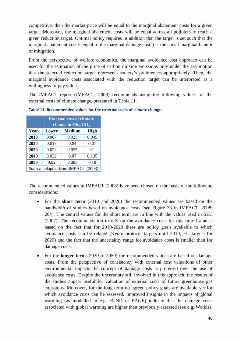
40
competitive, then the market price will be equal to the marginal abatement costs for a given target. Moreover, the marginal abatement costs will be equal across all polluters to reach a given reduction target. Optimal policy requires in addition that the target is set such that the marginal abatement cost is equal to the marginal damage cost, i.e. the social marginal benefit of mitigation.
From the perspective of welfare economics, the marginal avoidance cost approach can be used for the estimation of the price of carbon dioxide emissions only under the assumption that the selected reduction target represents society’s preferences appropriately. Then, the marginal avoidance costs associated with the reduction target can be interpreted as a willingness-to-pay value.
The IMPACT report (IMPACT, 2008) recommends using the following values for the external costs of climate change, presented in Table 11.
Table 11. Recommended values for the external costs of climate change.
External cost of climate change in €/kg CO2
Year Lower Medium High 2010 0.007 0.025 0.045 2020 0.017 0.04 0.07 2030 0.022 0.055 0.1 2040 0.022 0.07 0.135 2050 0.02 0.085 0.18 Source: adapted from IMPACT (2008)
The recommended values in IMPACT (2008) have been chosen on the basis of the following considerations:
• For the short term (2010 and 2020) the recommended values are based on the bandwidth of studies based on avoidance costs (see Figure 33 in IMPACT, 2008: 264). The central values for the short term are in line with the values used in SEC (2007). The recommendation to rely on the avoidance costs for this time frame is based on the fact that for 2010-2020 there are policy goals available to which avoidance costs can be related (Kyoto protocol targets until 2010, EC targets for 2020) and the fact that the uncertainty range for avoidance costs is smaller than for damage costs.
• For the longer term (2030 to 2050) the recommended values are based on damage costs. From the perspective of consistency with external cost valuations of other environmental impacts the concept of damage costs is preferred over the use of avoidance costs. Despite the uncertainty still involved in this approach, the results of the studies appear useful for valuation of external costs of future greenhouse gas emissions. Moreover, for the long term no agreed policy goals are available yet for which avoidance costs can be assessed. Improved insights in the impacts of global warming (as modelled in e.g. FUND or PAGE) indicate that the damage costs associated with global warming are higher than previously assessed (see e.g. Watkiss,

41
2005; and Stern, 2006), especially in the light of possible non-linear, dramatic effects that may occur in the longer term. In recent literature therefore a trend towards higher damage cost values can be observed.
IMPACT (2008: 82) underlines that “it should be highlighted here that CO2 reduction targets vary from country to country and that also the translation of national targets to targets per sector may be different between countries. Furthermore also CO2 avoidance costs may differ from country to country. As such external costs defined on the basis of avoidance costs could be made country specific.” Despite this recommendation, in the EFORWOOD project we adopt uniform price for CO2 and we do not differentiate it on a country by country basis. The knowledge base for doing that is found to be insufficient currently.
4.3.4 Monetary estimates for CO2 adopted for the use in EFORWOOD
Table 12 represents the monetary estimates in €/kg of CO2 eq. to be used for monetary valuation of GHG gases and carbon sequestration in the EFORWOOD project. The values for the year 2005 are based on the collected studies, and they are in line with the spot prices of CO2 in ETS in 2005. The values for 2010 and beyond are based on the recommendations of the IMPACT (2008).
Table 12. Adopted values for GHG emissions and carbon sequestration.
Year €/kg CO2
Lower value
Central value
Upper value
2005 0,004 0,011 0,021 2010-2019 0,007 0,025 0,045 2020-2029 0,017 0,040 0,070 2030-2039 0,022 0,055 0,100 2040-2049 0,022 0,070 0,135
2050 0,020 0,085 0,180

42
Table 13. A database of reviewed valuation studies.
Study Object Method 1991-2000 2001-2010 2011-2020 2021-2030 Currency Remarks Selected values for 2001-2010 €/tC in
2000 prices Min Max
Selected values for 2001-2010 €/tC in 2000
prices Min Max
Nordhaus (1991) PRTP = 1%
Marginal damage costs
Marginal Cost 10.74 €/tC €2000
0% upper limit, 4% lower limit
10.74
2.93
PRTP = (0%, 4%) 3.26 -211.48 €/tC 3.26 211.48 0.89 57.72
Ayres and Walter (1991) Marginal damage costs
Marginal Cost 41.67 – 48.61 €/tC €2000
Peck and Teisberg (1992) PRTP=3%
Marginal damage costs
Cost Benefit Analysis
14.6 -17.58 €/tC 17.58 – 20.51 €/tC
20.51 – 26.36 €/tC
26.37 – 32.22 €/tC
€2000
Nordhaus (1992, 1994) PRTP=3% Best guess
Marginal damage costs
Cost Benefit Analysis
7.77 €/tC 9.98€/tC 12.58€/tC 14.65€/tC
€2000
13.88€/tC for 2021-2030 according to Pearce (2000)
9.98 2.72
Expected value 17.58€/tC 26.37€/tC 26.36€/tC N/A 26.37 7.2
Cline (1992, 1993) SRTP=0%
Marginal damage costs
Cost Benefit Analysis
181.71€/tC
225.70€/tC
272.3€/tC
323.83€/tC €2000
225.70
61.60
SRTP=10% 8.46€/tC 11.18€/tC 14.32€/tC 17.25€/tC 11.18 3.05
Maddison (1994) SRTP=5%
Marginal damage costs
Cost Benefit Analysis
8.70€/tC 11.83€/tC 16.30€/tC 21.60€/tC
€2000
11.83 3.23
Marginal Cost 8.91€/tC 12.26€/tC 16.82€/tC 22.24€/tC 12.26 3.35
Fankhauster (1994) PRTP=0%
Marginal damage costs
Marginal Cost 29.73€/tC 33.42€/tC 37.10€/tC 40.69€/tC
€2000
33.42
9.12
PRTP=(0.5%, 3%) 9.12 – 66.18€/tC 10.85 – 77.47€/tC
12.15 – 85.60€/tC
13.45 – 94.06€/tC
10.85 77.47 2.96 21.14
Schauer (1995) Expert, parameters
12.15€/tC €2000
12.15
3.32
Expert, direct 156.25€/tC 156.25 42.65
IPCC (1996) Marginal damage costs
5 – 125€/tC 7 – 154€/tC $1990 9.77 213.76 2.67 58.34
6 – 160€/tC 9 – 197€/tC €2000
Plambeck and Hope (1996) PRTP=2%
PAGE model 63.91€/tC
€2000
PRTP=3% 29.19€/tC
Dames and Moore (1999) Marginal abatement cost
85.72€/tC €2000

43
Tol (1999), FUND 1.6 SRTP=5%
Marginal Cost 16.17€/tC 18.99€/tC 21.92€/tC 26.36€/tC €2000
Roughgarden and Schneider (1999)
DICE model 7.27 – 16.17€/tC 8.79 – 18.99€/tC
11.72 – 23.43€/tC
14.65 – 30.81€/tC
€2000
Nordhaus and Boyer (2000) SRTP=3%
Marginal damage costs
Cost Benefit Analysis
6.94€/tC 9.87€/tC. 12.91€/tC 16.30€/tC €2000
9.87 12.91 2.69 3.52
Study Object Method 1995 – 2004 2005 - 2014 Currency Remarks 2005-2014
Eyre et al (1999), Tol (1999) SRTP=1% Best guess:
Marginal damage cost
Marginal Cost
FUND 1.6 OF FUND 1.6 OF
FUND 1.6 model, documented in Eyre et al (1999) and in Tol (1999)
FUND 1.6 OF
Equity weighted 276.64€/tC 264.70€/tC 277.78€/tC 286.4€/tC €2000 277.78 286.46 75.81 78.18
No equity weighted 118.25€/tC 119.33€/tC 129.12€/tC 130.21€/tC €2000 129.12 130.21 35.24 35.54
SRTP=3% Best guess:
Equity weighted 118.25€/tC 125.84€/tC 126.95€/tC 148.66€/tC €2000 126.95 148.66 34.65 40.57
No equity weighted 45.57€/tC 57.50€/tC 53.17€/tC 68.36€/tC €2000 53.17 68.36 14.51 18.66
SRTP=5% Best guess:
Equity weighted 61.84€/tC 85.70€/tC 70.53€/tC 105.25€/tC €2000 70.53 105.23 19.25 28.73
No equity weighted 21.70€/tC 4014€/tC 27.12€/tC 51.00€/tC €2000
Study Object Method 2000-2009 Currency Remarks 2000-2009
Tol and Downing (2000)
Marginal damage cost
Marginal Cost
VLYL VSL Ref. Pearce (2000) VLYL = value of a year of life lost VSL= value of a statistical life
VLYL VSL
PRTP=0% Best guess 17.25€/tC 31.46€/tC 21.37€/tC €2000 17.25 31.47 4.71 8.59
PRTP=1% Best guess 10.20€/tC 14.32€/tC 3.8€/tC €2000 10.20 14.32 2.78 3.91
PRTP=3% Best guess 4.34€/tC 1.52€/tC -7.38€/tC €2000
Tol (2005) PRTP=3% 7$/tC $1995 PRTP=1% 33$/tC $1995 PRTP<=0% 39$/tC $1995
Defra (2007) Based on Stern Review (2006) and stabilization level of 550ppm CO2 eq
Social cost of carbon
32.55€/tCO2 €2000
Shadow price of carbon
35.79€/tCO2 €2007

44
Blok et al. (2001) EU wide
Shadow price for CO2
Marginal abatement costs in 2010
20 - 42€/tCO2 eq
€1999
Davidson et al. (2002) Netherlands
Shadow price for CO2
National cost estimates
50€/tCO2
Study Object Method €2000 prices Min Max
€2005 prices Min Max
Remarks
Defra (2002) Social cost of carbon
Min 14€/tCO2 57.49€/tC 18€/tCO2 65.82€/tC Assumes annual increase in real terms of 1€/tC
Max 56€/tCO2 229.97€/tC 66€/tCO2 239.88€/tC
Central value 28€/tCO2 114.98€/tC 34€/tCO2 124.33€/tC
ExternE (2005) Avoidance Cost
Min 5€/tCO2 eq 18€/tCO2 eq
*calculated using marginal damage cost
Max 20€/tCO2eq 24€/tCO2 eq
Central Value 9€/tCO2 eq * 19€/tCO2 eq
McKensey (2007) Estimates that in 2030, a stabilisation target of 550ppm would require a carbon price of 25€/tCO2, and a target of 450ppm would require a carbon price of 40€/tCO2 (2007 price) but would only be applied only in 2030.
Notes: All values adapted from sources using the OECD Average annual exchange rates PRTP = Pure rate of time preference SRTP = Social rate of time preference

45
4.4 Water pollution
Forest watersheds perform an important ecosystem service in terms of maintenance and enhancement of protective functions in the provision of water resources. Water supply is becoming an increasingly important issue for water resource managers and planners as demands for water continue to increase. Water consumption is increasingly seen as a basic indictor for sustainability assessments of a region.
Climate change predictions for warmer and drier summers will put further pressure on supplies. Jointly with climatic variation, forest cover and structure, site conditions, species composition, roads, skid trails will cause a high variation of the response of water yield to treatments. To uncover the effects of forest management and related processes on the water cycle, changes can be measured in EFORWOOD in terms of of water quality (indicator 18), and emissions to water (indicator 21).
The focus of this section is the valuation of Nitrogen (N) and Phosphorous (P) emissions to the aquatic environment in a European context. The purpose is to derive from the literature a range of value estimates for N and P emissions, which can be used in the EFORWOOD framework for forest wood chain assessments.
The research is based on a review of European studies on valuation of N and P emissions to the aquatic environment. The reviewed studies apply a range of valuation methodologies such as abatement costs (e.g. Brady, 2003; Byström, 1998; Huhtala and Marklund, 2008; Nunneri et al., 2007; and Turner et al., 1999), contingent valuation (e.g. Atkins and Burdon, 2006; Gren et al., 1997b; Stenger and Willinger, 1998), hedonic pricing and travel cost estimation (e.g. Sandström, 1996).
Geographically the review includes studies from Finland (Helin et al., 2006; Laukkanen and Huhtala, 2008; Lehtonen et al., 2007; Huhtala and Marklund, 2008), Sweden (Sandström, 1996; Byström, 2000; Byström et al. 2000; Byström 1998; Brady, 2003), Denmark (Atkins and Burdon, 2006; Münier et al., 2004; Jacobsen, 2002; Jacobsen et al., 2005; Berntsen et al., 2003), Germany (Nunneri et al., 2007), the Baltic sea region as such, including Sweden, Denmark, Germany, Poland, Estonia, Latvia, Lithuania, St Petersburg and Kaliningrad (Turner et al., 1999; Elofsson, 2006; Gren, 1999; Gren et al., 1997a; Gren et al, 1997b), the Netherlands, Czech Republic (Nunneri et al., 2007), Croatia (Sumelius et al., 2003), France (Le Goffe, 1995; Stenger and Willinger, 1998; Rinaudo et al., 2005) and England (Kampas and White, 2004).
4.4.1 Changes in the water processes
The indicator values assigned to any of the FWC-processes under the reference futures (A1 and B2), respectively should ideally reveal any increase or decrease in quality and quantity of water, e.g. groundwater discharge and surface water run-offs, and what the impacts on health for those populations that rely on the availability of freshwater, groundwater, coastal and marine zones (e.g. through the discharge of sewage, algae concentrations, nutrients, oil, heavy metals and other pollutants). Issues related to emissions to water are also directly related within each Module (M2-M5) to environmental impacts of transport (throughout M2 to M5, see Section 4.5), waste (throughout M4-M5, see Section 4.6), forest management (in M2 for further information see D2.2.2, 2009) and wastewater emissions (throughout M2 to M5, see

46
Section 4.6) classified by organic substances (BODs), nutrients (nitrogen, phosphorus), and hazardous substances.
Information on water process for individual countries or chains is not available in terms of the expected changes from the scenarios and reference. However, information on how the changes will generally influence the FWCs is available for the EU-FWC in D 1.4.7 (2008), for the Scandinavian FWC in PD 2.0.5 (2007), for the Baden-Württemburg FWC in PD 3.0.3 (2007) and in terms of forest resource management in D 2.2.2 (2009).
The future scenarios are likely to have substantial consequences on the quality and quantity of water when considering that the main drivers include population, industrial productivity, climate change, and changing water use. In A1 reference future, increases in runoff are likely, especially with heavy concentrations of BODs and N and P concentrations, as a result from land use change and a move away from forestry towards agricultural productivity. Evidence of this kind of potential change would provide a useful illustration that land use and industrial changes are important factors in future water resource changes.
Given the higher temperatures, particularly in summer, and more winter precipitation along coasts (except for the Mediterranean) and in mountain ranges (except for the Pyrenees), there is likely to be a shift in the forest types under B2 reference future as soil water supply is sharply reduced for the vegetation. Water storage capacity of soils in forest areas and local conditions in terms of nutrient supply will be key factors in governing emissions to water (Lousteau, 2001).
4.4.2 Economic values of N and P emissions in EFORWOOD context
When suggesting value estimates for the use in the cost-benefit analysis, we are restricted by the requirements implied by EFORWOOD framework. This includes, that data and approaches have to be relatively comparable to allow for cross-European applications, and quite importantly we need to focus our attention to the fact that estimates have to be provided or possible to transform into a useful unit, i.e. EUR/kg nutrient.
Ideally, welfare economic measures, reflecting use and non-use values related to aquatic N and P emissions should be used in the EFORWOOD framework. Provided the above argumentation on general applicability, this implies that cross-European welfare economic surveys ought to be carried out. In order to ensure comparability, these surveys should use the same methodology to assess aquatic N and P emissions in all cases. Also this exercise, however, is beyond the time and resource provisions of the CBA-work in EFORWOOD. A literature review of existing surveys has been carried out instead as a basis for value transfer.
The majority of the reviewed literature use abatement costs to assess the value of aquatic N and P emissions. It is suggested that the value estimates to be used in EFORWOOD are based on these abatement cost assessments. The strengths of using abatement costs are that estimates are, relative to e.g. contingent valuation estimates, comparable, they reflect actual market prices of marketed goods and – quite important for our purpose - they are often presented in EUR/kg, which makes them readily applicable in EFORWOOD.
Some of the weaknesses of abatement cost estimates are that they, as opposed to welfare economics measures obtained e.g. as contingent valuation estimates may not reflect the welfare change caused by the abatement. In this way abatement cost estimates in most cases

47
do not reflect the true welfare economic value of the goods assessed. If abatement is optimal for society, then they represent a conservative substitute for a true value measure. Thus, when used in the context of EFORWOOD, for example, abatement cost estimates reflect a minimum value of the environmental change assessed.
4.4.2.1 Abatement cost estimates for N and P emissions
The majority of abatement cost studies combine different types of agro-ecological/hydrological models with economic optimisation and stakeholder behaviour models. This is done to assess marginal costs related to either specific abatement measures, to a set of abatement scenario alternatives and/or to specific abatement targets.
Table 14 outlines the part of reviewed literature that specifies marginal abatement costs of N and P emissions to the aquatic environment in EUR/kg N or P. The abatement measures assessed in the reviewed literature are related to agricultural/land use practises like wetland establishment, animal husbandry, livestock feed and fertiliser use. They are also related to technical abatement solutions, like construction of sewage treatment plants and manure storage and to policy measures like N-taxes and set-aside subsidies.
The use of the abatement cost estimates in EFORWOOD is suggested bearing in mind the heterogeneity of methods used and aims of the reviewed literature. Some studies assess costs for specific abatement targets like 50% or 25% reduction of emissions, see e.g. Gren et al. (1997a), Helin et al.(2006) and Elofsson (2006). In these studies, marginal costs increase with abatement targets i.e. the last 10% of a 50% abatement target are more costly than the first 10%.
Other studies assess costs for specific policy packages like CAP12 and DAP13
From this follows that abatement cost estimates vary depending on where, how and which abatement measures are implemented. Country specific input factor prices, local biophysical characteristics and land use practises very much influence the effectiveness and costs of an applied abatement measure. In the EFORWOOD context this means that not a single abatement cost value will be suggested. Rather, a range of abatement cost estimates, based on the reviewed literature and depending on e.g. geographical location, biophysical characteristics and the type of abatement needed, will be applied.
II and III, see e.g. Helin et al. (2006), Jacobsen (2002) and Jacobsen et al. (2005) respectively. The majority of these studies assesses costs of individual abatement measures separately, whether applied individually or in a policy package combination. Cost assessments for policy packages may thus be in the high end, as comparative advantages of combining various measures are considered only to a limited extend (Elofsson, 2006). On the other hand this makes cost estimates comparable at least with the literature that estimate costs of specific abatement measures separately, like the studies on wetland establishment, N-taxes, subsidies and sewage treatment plant, wetland establishment, land use changes, see e.g. Berntsen et al. (2003), Byström (1998), Gren et al. (1997a).
12 CAP: Common Agricultural Policy reform 13 DAP: Danish Aquatic Programme

48
Table 14. Abatement cost estimates provided in the reviewed studies on N and P emissions.
Study Year Focus of study Abatement cost estimates Elofsson 2006 Costs of reducing N and P emissions to
the Baltic Proper by 25% Marginal costs of 25% reduction: N-abatement: 0.4 – 1.4 EUR/kg N, P-abatement
Helin et al.
: 1.4 – 9.7 EUR/ kg P 1
2006 Cost of Common Agricultural Policy (CAP) abatement measures, Finland: 50% reduction of N and P emissions through changed agricultural practises
Abatement costs of 50% reducing in N-load: CAP 2003: 9,4 EUR/ kg N. CAP 2006
Huhtala and Marklund
: 7,2 EUR/kg N
2008 Costs of manure regulations as water protection (P-abatement) measures in Finland
Shadow price of establishing nutrient limits: 60-125 EUR/ kg P
Jacobsen et al.
2005 Marginal costs of abatement measures included in Danish Aquatic Programme (DAP) II, Denmark.
Marginal costs of DAP III, 13% N-reduction compared to DAP II: 2.5-3.5 EUR/kg N
Berntsen et al.
2002 Marginal costs of different taxation schemes, aimed at N-abatement in Denmark.
Social abatement costs of different N-taxation policies: 1-9 EUR/kg N
Brady. 2003 Cost of abatement measures in Sweden: Uniform N-tax, green subsidies, land-use regulation
Marginal abatement costs
Jacobsen
(scenarios: standard, coordinated): 1.1 EUR/kg coastal N, -1.3 EUR/kg coastal N 2.
2002 Marginal costs of abatement measures included in DAP II, Denmark.
Avg. abatement costs: 3.1 EUR/kg N/yr
Turner et al.
1999 Cost of abatement measures in the Baltic Proper, costs depend on activity and country. - Emission reduction from agriculture - Sewage treatment plant
establishment - Reduction of air emissions - Wetland establishment
Cross country average N-abatement costs: agriculture: 4.4-21.9 EUR/kg N, sewage treatment: 2.7-5.2 EUR/kg, wetlands:
Cross country average P-abatement costs:
1.4-7.5 EUR/kg N (avg.: 3.2 EUR/kg N)
agriculture 23.8-532 EUR/kg P, sewage treatment: 4.7-9.5 EUR/kg P, wetlands
: 61.9-2069.5 EUR/kg P (avg.: 367 EUR/kg P)
Byström 1998 Abatement costs of wetland establishment in Sweden
Marginal abatement costs for high-leaching and low-leaching scenario respectively: 2.2 – 3.1 EUR/kg N 4
Gren et al.
1997a Marginal costs of 50% reduction of N and P emissions to the Baltic Proper. Abatement measures include land use changes and nutrient retention.
N-abatement costs (cross Baltic range): Land use: 2.3 – 96.3 EUR/kg N, retention: 1.6 – 61.5 EUR/kg N. P-abatement costs (cross Baltic range): Land use: 28.5 – 776.8 EUR/kg P, retention:
Notes: 1 1EUR=9,25 SEK (2006) 21 EUR =9.13 SEK (2003) 31 EUR = 8,81 SEK (1999) 23.4 – 117.2 EUR/kg P 5
41 EUR=8.93 SEK (1998) 5 1EUR=8,62 SEK (1997)
4.4.2.2 Costs of N-abatement in the EFORWOOD context
In the reviewed literature, the positive correlation between opportunity costs of input factors and abatement costs is well documented. An example is Jacobsen (2002). In this article a range of cost estimates for agricultural N-abatement measures in Denmark are presented. Average costs of the three most expensive abatement measures are 15.1 EUR/kg N. The measures are organic farming (19.9 EUR/kg N), ESA area management (10.4 EUR/kg N) and reduced stocking density (15 EUR/kg N), all abatement measures with high opportunity costs.

49
In comparison, the average of other abatement measures included in the study is 1.8 EUR/ kg N.
The argued implications of geographical variance for abatement costs are also well described in the reviewed literature. Turner et al. (1999) illustrate this in their presentation of abatement cost estimates across the Baltic countries. Noteworthy are the costs of wetland establishment for P-abatement. In Sweden costs of wetland establishment are 2069 EUR/kg P. In comparison, average costs in the other countries included in the study are 178 EUR/kg P. The reason for this is that wetlands have already been extensively established in Sweden, and additional wetlands have to be established on more productive lands at high marginal opportunity costs.
The literature on costs of administrative regulation of N and P emissions, like tax schemes and nutrient limits, also use opportunity costs of input factors and production output as base for abatement cost estimates (see e.g. Berntsen et al., 2003; Huhtala and Marklund, 2008; Brady, 2003; Jacobsen, 2002; Jacobsen et al., 2005). Costs of administration and enforcement of a given regulation initiative are included in the reviewed literature only to a limited extend. Though such administrative cost estimates would have been useful, the advantage of the prevailing abatement cost estimates is that they are readily comparable with the cost estimates other types of assessments.
The N-abatement costs presented in table 1.1 are between 0.4 and 96.3 EUR/kg N. Cost estimates in the high end of the scale are presented by Gren et al. (1997a). Abatement costs are here estimated for 50% reduction of N and P emissions to the Baltic Sea and land use measures are some of the most costly in this study. This supports the argumentation of positive correlation between abatement costs and opportunity costs of, in this case, land. A 50% reduction of emissions will require that land and land use practises with high productivity and hereby high opportunity costs are included in the abatement efforts, together with the less productive lands and practises, to achieve the 50% reduction.
4.4.2.3 N-abatement cost ranges suggested for the use in EFORWOOD
In the EFORWOOD context it is suggested to allow the end-user to use different N abatement cost estimates depending on the particular process being assessed. Embracing the indications that especially land-use/agriculturally related N abatement costs increase with the opportunity costs of input factors, it can be argued that costs related to the early stage processes (e.g. regeneration and felling) in FWC are in general lower than cost related to the later stage processes (e.g. sawmill and processing). In other words, the cost of N emissions taking place in relation to the close-to-forest FWC processes will be at the low end of the scale as they take place on more marginal lands with lower opportunity costs. As the FWC processes move towards more fertile areas, with more specialised land use practises and industries, opportunity costs and hereby abatement costs related to N emissions will likely increase.
It is therefore suggested to use different ranges of abatement cost estimates, depending on which type of FWC process is being analysed. Based on reviewed literature, the following cost ranges for N emissions are suggested:
1) Low range: 0.5 – 5 EUR/kg N. Includes abatement measures with low opportunity costs like inclusion of marginal lands e.g. for wetland establishment, low cost change

50
of land use practises and low cost improvements of existing sewage treatment systems (e.g, Turner et al., 1999; Jacobsen, 2002; Byström, 2000)
2) Middle range: 5 – 20 EUR/kg N. Includes abatement measures with medium size opportunity costs like change in land use practises e.g. the time of manure spreading and use of catch crops on productive agricultural lands and medium cost changes in animal husbandry practises like lower stocking density (e.g. Gren et al., 1997a; Berntsen et al., 2003)
3) High range: 20 – 90 EUR/kg N. Includes measures with high opportunity costs like organic farming (e.g. Jacobsen, 2002), change in highly productive land use and animal husbandry practises like decreased livestock holdings, introduction of fallow and establishment of buffer strips (e.g. Elofsson, 2006, Huhtala and Marklund, 2008; Gren et al., 1997a) as well as, e.g. sewage treatment from industrial waste water.
4.4.2.4 Costs of P-abatement in the EFORWOOD context
The measures applied for reduction of P emissions are the same types of measures mentioned above for N abatement e.g. wetland establishment, change in land use and animal husbandry practises, sewage treatment, see e.g. Gren et al. (1997a); Turner et al. (1999) and Elofsson (2006). A number of the measures suggested for abating N emissions also have implications for the emissions of P and vice versa. Estimates for costs of joint reduction of N and P emissions may thus be much lower than abatement cost estimates for N and P individually.
Abatement cost estimates for P reduction are provided by a.m.o. Elofsson (2006) Huhtala and Marklund (2008), Turner et al. (1999) and Gren et al. (1997) and they are outlined in Table 14. The table shows a span of P abatement cost estimates between 1.4 and 776.8 EUR/kg P with the low end of the scale being between 1.4 and 28.5 EUR/kg P and the high end of the scale being between 60 and 776.8 EUR/kg P. The somewhat higher cost estimates for P abatement, compared to N abatement costs, is explained by the properties of P as a much less mobile and soluble nutrient than N, implying that much less is transported pr area or soil water volume. Higher costs are therefore associated with the abatement of P. On the other hand it is argued that P can be regarded as a keystone pollutant meaning that if P is managed then the eutrophication effect of N will also be reduced, which is not always the case the other way around (Turner et al., 1999; Elofsson, 2006).
Like the N abatement cost estimates, P abatement costs are positively correlated with the marginal opportunity costs of the abatement measures applied. The costs using sewage treatment for P abatement are within the same range as for N abatement, i.e. 20 – 100 EUR/kg. Where sewage treatment is one of the marginally more expensive measures for N abatement, it is the most cost efficient measure for P abatement compared to land use and animal husbandry related abatement (Turner et al., 1999).
4.4.2.5 P-abatement cost ranges suggested for the use in EFORWOOD
As for abatement costs related to N emissions, it is suggested to use different ranges of cost estimates for P abatement. The cost ranges will take point of departure in the opportunity costs of the different measures and their application will depend on the particular FWC process being assessed. This means that the cost of P emissions taking place in relation to the

51
close-to-forest FWC processes will be at the low end of the scale. As the FWC processes move towards more fertile areas, with more specialised land use practises, opportunity costs and hereby abatement costs related to P emissions will increase.
As for N abatement, the ranges for P abatement will depend on which type (high or low opportunity costs) of FWC process is being analysed and in which geographical location. Based on reviewed literature, the following cost ranges for P emissions are suggested:
1) Low range: 1.5 - 60 EUR/ kg P. Includes abatement measures with low opportunity costs like decrease in fertilisers on less productive lands (Elofsson, 2006), changes in manure management (Huhltala and Marklund, 2008) and sewage treatment (Turner et al., 1999)
2) Middle range: 60 – 300 EUR/kg P. Includes abatement measures with medium opportunity costs like change in livestock holdings (Elofsson, 2006) and wetland establishment14
3) High range: 300 – 760 EUR/kg P. Includes abatement measures with high marginal opportunity costs like wetland establishment in Sweden (Turner et al., 1999) and land use changes e.g. from high leaching to low leaching crops (Gren et al., 1997a).
(Turner et al., 1999)
4.4.2.6 Benefits of nutrient abatement
As mentioned in Section 4.4.2, a cross European economic study on the welfare economic value of N and P emissions, where value estimates were comparable across countries and denoted in EUR/kg nutrient, would have been ideal for use in the EFORWOOD project. As present resource provisions do not allow for the realisation of this ideal situation, the above mentioned use of abatement cost estimates in EFORWOOD is considered a second best solution.
This is done bearing in mind that abatement cost estimates do not describe all welfare economic changes in use and non-use values related to changes in aquatic N and P emissions. This should be acknowledged when using the suggested abatement cost ranges in EFORWOOD. In an attempt to put abatement cost estimates into a larger welfare economic perspective, literature on welfare economic assessments of nutrient emissions to the aquatic environment in Europe has been reviewed. Table 15 outlines the welfare economic values related to nutrient emissions. All but one study base value estimates on contingent valuation studies carried out for a specific abatement scenario in a specific country/region, e.g. 50% and 80% reduction in N and P emissions respectively to Randers Fjord in Denmark (Atkins and Burdon, 2006) or the restoration of Brest natural harbour in France (Le Goffe, 1995).
Table 15 shows substantial values attributed to improvements of water quality, for drinking water purposes as well as for recreational purposes. From EFORWOOD point of view, the value estimates in Table 15 are not applicable as they reflect values that are specific for the site and abatement scenario for which they have been assessed. Value transfers of such estimates are therefore only feasible in cases very similar to the ones assessed and therefore of little use in the EFORWOOD context, which in many ways is much broader. Moreover,
14 Except for in Sweden where costs related to wetland establishment for P abatement are much higher (Turner et al.; 1999)
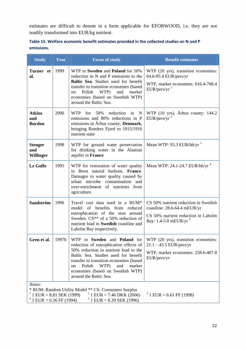
52
estimates are difficult to denote in a form applicable for EFORWOOD, i.e. they are not readily transformed into EUR/kg nutrient.
Table 15. Welfare economic benefit estimates provided in the collected studies on N and P emissions.
Study Year Focus of study Benefit estimates
Turner et al.
1999 WTP in Sweden and Poland for 50% reduction in N and P emissions to the Baltic Sea. Studies used for benefit transfer to transition economies (based on Polish WTP) and market economies (based on Swedish WTP) around the Baltic Sea.
WTP (20 yrs), transition economies: 64.6-95.4 EUR/pers/yr
WTP, market economies: 616.4-768.4 EUR/pers/yr 1
Atkins and Burdon
2006 WTP for 50% reduction in N emissions and 80% reductions in P emissions in Århus county, Denmark, bringing Randers Fjord to 1915/1916 nutrient state
WTP (10 yrs), Århus county: 144.2 EUR/pers/yr 2
Stenger and Willinger
1998 WTP for ground water preservation for drinking water in the Alsatian aquifer in France
Mean WTP: 93.3 EUR/hh/yr 3
Le Goffe 1995 WTP for restoration of water quality in Brest natural harbour, France. Damages to water quality caused by urban microbe contamination and over-enrichment of nutrients from agriculture.
Mean WTP: 24.1-24.7 EUR/hh/yr 4
Sandström 1996 Travel cost data used in a RUM* model of benefits from reduced eutrophication of the seas around Sweden. CS** of a 50% reduction of nutrient load in Swedish coastline and Laholm Bay respectively.
CS 50% nutrient reduction in Swedish coastline: 28.6-64.4 mEUR/yr
CS 50% nutrient reduction in Laholm Bay: 1.4-3.8 mEUR/yr 5
Gren et al. 1997b WTP in Sweden and Poland for reduction of eutrophication effects of 50% reduction in nutrient load to the Baltic Sea. Studies used for benefit transfer to transition economies (based on Polish WTP) and market economies (based on Swedish WTP) around the Baltic Sea.
WTP (20 yrs), transition economies: 21.1 – 43.5 EUR/pers/yr
WTP, market economies: 258.6-407.8 EUR/pers/yr
Notes: * RUM: Random Utility Model ** CS: Consumers Surplus 1 1 EUR = 8,81 SEK (1999) 2 1 EUR = 7.46 DKK (2006) 3 1 EUR = 6.61 FF (1998) 4 1 EUR = 6.56 FF (1994) 5 1 EUR = 8.39 SEK (1996)

53
4.4.3 The EFORWOOD chains and attributed water pollution costs
In general reviewed literature provides cost estimates for the following abatement measures:
• Land use conversion – cost estimates are mainly provided for wetland establishment and based on opportunity costs of land
• Agricultural production change – cost estimates provided for opportunity costs and costs of input factors related to changes in agricultural production procedures like cropping patterns, livestock density, livestock feed and manure spreading
• Establishment of sewage treatment – cost estimates provided for new establishments and improvements of existing sewage treatment facilities. Abatement cost estimates are based on costs of input factors and production related opportunity costs
In the EFORWOOD indicator set, water pollution is dealt with in two sub-indicators: “24.1.1. Water pollution by organic substances”, measured in kg BOD5 per reporting unit, and “24.1.2. Water pollution by nutrients as nitrogen”, measured in kg TKN. TKN is a measure of total extractable nitrogen from the matter – using the Kjeldahl method (Total Kjeldahl Nitrogen). TKN is not exactly the same measure as the kg N referred to in almost all the studies we rely on here. They consider mainly the in-organic fraction of N in the waterbodies. The TKN measure includes nitrogen on its in-organic forms, e.g. dissolved ammonium compounds, nitrate etc., as well as nitrogen tied in an organic matrix. It is the former that is the polluting form, as it works directly as a nutrient for organisms and may lead to damaging levels of eutrophication and it is also the form, which can be a health risk, e.g. nitrate is considered a carcinogen factor at high levels. However, as we are here considering TKN in emissions to water, it is fairly safe to assume that kg TKN is very close to kg inorganic N. The organically tied fraction is likely to be little and furthermore, under the usual aerobe conditions in water, the organic substances are likely to be oxidised within a short while, converting organically tied nitrogen to in-organic solvents of N.
In the following, specific abatement cost estimates are suggested for the individual Modules within the EFORWOOD project.
4.4.3.1 Module 2: Forest resource management
The costs of water pollution in this part of the chain depend on whether the forest is located on (potentially) productive or marginal lands. In the mid-term evaluation of the Danish Aquatic Programme II, forests are the second most cost efficient (3.1 EUR/kg N) abatement measure under the programme. The most cost efficient measure is wetlands (0.7 EUR/kg N) (Jacobsen, 2002).
As shown by e.g. Gren et al. (1997) and Turner et al. (1999) costs related to abatement measures such as land use conversions (e.g. from agriculture to forests or wetlands) are, however, determined by the opportunity costs of land. These costs vary between sites. The estimates of Jacobsen (2002) are in many ways site specific and it is suggested not to use these estimates in the forest resource management module.
It is instead suggested to use abatement costs for land use conversion such as wetland establishment, which are provided in the literature reviewed in relation to Note 1. One argument for this is that cost estimates for wetland establishment are provided for several

54
geographical regions and is therefore considered as more generally applicable approximations than Jacobsen (2002).
Based on reviewed abatement costs (primarily for wetland establishments and set aside land), following costs are suggested for processes in forest resource management chain:
For N abatement, if opportunity costs of land are:
• Low, use 3 EUR/kg N;
• Medium, use 6 EUR/ kg N; and
• High, use 40 EUR/kg N.
For P abatement, if opportunity costs of land are:
• Low, use 40 EUR/kg P;
• Medium, use 60 EUR/kg P; and
• High, use 300 EUR/kg P.
The use of suggested ranges in the EFORWOOD project requires from the user that he/she has insight into the opportunity costs of land in relation to the specific process. If the user has no knowledge on the opportunity costs of land, it is suggested that the medium value is used as a default.
4.4.3.2 Module 3: Forest to industry interactions
This part of the chain deals mainly with the storage and transportation of forest products from the forest to a given processing site. The costs of water pollution here would mainly be related to emissions from transport vehicles and storage facilities and abatement measures would be changes in vehicle and/or storage technology and in polluting transport and storage procedures. Abatement cost estimates would be based on costs of input factors to technological abatement and to opportunity costs of production related to pollution abating changes in procedures.
Such data for forest to industry interactions are not readily available, and is often not reported on in the indicators set for this part of the FWC. If, in a concrete scenario examined, emissions are expected, and they are likely to be through road run-off or the like, the suggested costs for Module 4 level processes are recommended. If the emissions are expected to be more diffuse in the landscape, then those of Module 2 should be used.
4.4.3.3 Module 4: Industrial processing and manufacturing
In this part of the chain it is suggested to use the cost estimates for sewage treatment, which are presented in the reviewed literature, as approximations for abatement costs. The validity of this approximation is apparent for e.g. the pulp industry where sewage treatment is an indeed relevant measure for water pollution abatement. Cost estimates are in this part of the chain related to the scale of investment in abatement measures and to the opportunity costs of foregone production related to abatement activities.

55
Based on reviewed abatement costs (primarily for sewage treatment and agricultural production foregone), following costs are suggested for processes in the industrial processing and manufacturing part of the chain:
For N abatement, if costs of abatement technology and production foregone are:
• Low, use 4 EUR/kg N;
• Medium, use 10 EUR/kg N; and
• High, use 20 EUR/kg N.
For P abatement, if costs of abatement technology and production foregone are:
• Low, use 9 EUR/kg P;
• Medium, use 25 EUR/kg P; and
• High, use 300 EUR/kg P.
In the application of suggested cost ranges for this part of the chain, the user needs knowledge on the scale of investments needed for water pollution abatement. If few improvements e.g. of existing sewage treatment facilities are needed, it is suggested to use the low end of the scale. If completely new pollution abatement facilities, like sewage treatment plants, have to be established, it is suggested to use the high end of the scale. It is suggested to use the middle range as default, if the user does not have the required knowledge on required abating investments.
4.4.3.4 Module 5: Industry to consumer interactions
In this module it can be argued that water polluting processes are mainly related to waste management (e.g. storage, recycling, combustion). In relation to this the water pollution abatement costs are determined by the technology and procedure changes required in the specific case. In the reviewed literature the most relevant approximations for abatement costs in this module are cost estimates related to sewage treatment and to some extent to the changes in agricultural production procedures like storage of animal manure.
The same ranges as for the Module 3 are therefore suggested. As in Module 3, the low range is used where little changes in existing pollution abating facilities are required and the high range is used where the establishment of new facilities is required.
Based on reviewed abatement costs (primarily for sewage treatment and agricultural production foregone), following costs are suggested for processes in the industry to consumer interaction process:
For N abatement, if costs of abatement technology and production foregone are:
• Low, use 4 EUR/kg N;
• Medium, use 10 EUR/kg N; and
• High, use 20 EUR/kg N.
For P abatement, if costs of abatement technology and production foregone are:
• Low, use 9 EUR/kg P;

56
• Medium, use 25 EUR/kg P; and
• High, use 300 EUR/kg P.
4.5 Transport externalities
4.5.1 Transport processes in FWCs
Transport modes are represented by road, rail and inland waterway throughout Europe. For the forest wood industry, their main purpose is to transport freight consisting of wood products such as particle boards, external walls, glulam, window frames, chairs and kitchen furniture. They also transport roundwood material, from species such as: Spruce; Douglas fir; Scots pine; Maritime pine; Black pine; Aleppo pine; Oak; Beech; Poplar; and Spanish chestnut.
Transport process in the FWC relate to three types of flows: (i) internal country flows; (ii) import / export flows within the EU; and (iii) import / export flows to and from extra- EU. The extra-EU flows correspond to the international flows in the Scandinavian and Iberian case studies. Transport is aggregated across modules throughout all transport process. In Module 3, the transported goods consist of wood and cork, and in Modules 4 to 5 the goods consist of construction material, pulp and paper, and manufactured goods. For further information refer to P.D. 3.3.6.
Data for rail flows are aggregated to the national and to the inter-Europe transport processes. Road transport is the most important form of transport in Europe, representing approximately 50% of the total EU freight transport, when international flows are integrated (P.D. 3.3.4). This mainly consists of heavy duty vehicles (HDV), which are trucks weighing from over 9 tons to 40 tons (the average for the FWCs in EFORWOOD of 26 tons). Light duty vehicles (LDV) are all motor vehicle ranging from anything less than 2.7 tons up to 12 tons (the average for the FWCs in EFORWOOD of 9 tons) (P.D.3.3.4).
Road transport
Table 16 represents the type of vehicles used at different stages of FWC, as reported in the Data Collection Protocol (PD0.0.16).
Our estimations for transport accidents for both HDV and LDV are based on the values found for HDV; this is due to the lack of homogenous and comparable information on transport accidents in LDV.
Table 16. Freight equipment for different FWC stages.
Harvesting Manufacturing Consumer
Heavy duty vehicle Roundwood Long logs
Chips
Semi-trailer Semi-trailer (Diesel)
Light duty vehicle - - Delivery lorries (Diesel)
Vans Diesel (mainly) vans Source: PD0.0.16.

57
Data for rail flows are aggregated to the national transport processes. The costs are attributed for train specific data to environmental (energy consumption and emissions), social (employment and wages) impact categories, and on a country specific level for the economic impact categories (share of production costs, share of GVA, cost distribution and production costs).
Rail transport
Data for shipping flows are aggregated to the international transport processes. Therefore, this includes domestic and international maritime transport, along coasts, rivers and lakes. The movement of cargo between ports situated in Europe, or with ports situates in non-EU countries that have a coastline bordering Europe, such as Iceland, states in the Baltic Sea, the Black Sea and the Mediterranean (P.D. 3.3.4). The costs are attributed to ship specific data for the environmental (energy consumption and emissions), social (employment and wages) impact categories, and on a country specific level for the economic (GVA, cost distribution and production costs) impact categories.
Inland waterway transport
In the context of the EFORWOOD project, currently there is no sufficient information at our disposal to make satisfactorily sound conjectures on the expected impact of scenarios under different reference futures for the analysed case studies. The available, albeit limited, information is regarding general description of reference futures. The general process is described in Timms et al. (2005) for A1 and B2 reference futures for 2050 and 2100 horizons adapted from IPCC (base year = 1995) (see P.D. 3.3.4 for further information), as well as in EFORWOOD D.1.4.7 (2008) for a specific description of changes in the forest wood chains (FWC).
Changes in transport processes
Reference futures Freight transport A1 Increased mobility B2 Decline due to use of local products
The following assumptions are applied to the storylines for the reference futures A1 and B2 in the transport process (P.D. 3.3.4):
• Wages and labour costs are updated accordingly with GDP growth rate;
• Labour productivity remains constant; and
• Working hours are assumed to remain the same.
Differences between A1 and B2 reference futures will be marked by the average distance and the modal distribution. The average distance and modal distribution in 2005 is estimated with macroeconomic data on transport of goods (wood and cork; pulp and paper; building material; manufactured products) in ton/km.

58
The transport of freight between 2015 and 2025 in A1 and B2 shows that the total tons-km loads rapidly increase in all scenarios. In the A1 reference future, freight demand increases by 3.2% per year, which is higher than the GDP growth rate. The total tons-km is higher in the policy scenarios than in the baseline scenario. This is particularly visible in the technology investments scenarios, because the policies in the demand regulation scenarios lead to a reduction of average trip lengths of the delivery of goods. Both rail and sea shipping need that goods are moved to and from terminals and the routes linking the terminals are generally longer than the road route. Concerning the future time steps, the indicator values as at a flow and transport mode level for 2015 and 2025 are explained by the distance and modal split change (cf. P. D. 3.3.4; P.D. 3.3.6).
On the level of the EU FWC, it is expected that under reference future A1, the high economic growth, free trade and limited environmental concern will cause road transport and air travel to grow rapidly. Improved logistics scheduling will reduce the costs for the transport sector. Where possible, road transport will be preferred above marine and rail transport, except in remote areas of Scandinavia. Little investment will be allocated to boat and train infrastructure facilities. The bulk of wood based material will be produced outside of Europe, but transport costs will be relatively low. (EFORWOOD D.1.4.7, 2008).
In contrast, in reference future B2, more people will tend to work from home, or choose to live closer to their work (rural areas staying populated), thus slightly reducing annual car use rates. Improved logistics scheduling will reduce costs from the transport sector. Rail and sea transport will be strong, and new industrial developments will be located in close proximity to these services. The forest industry will take advantage of new multi-modal forms of transport to minimize its costs (EFORWOOD D.1.4.7, 2008).
On the level of the Baden-Württemberg FWC, in 2005, the wood transported from the forest to the mill is split in the following way: 80% by truck; 50% by rail; and 5% by water. By 2015 and 2025, truck transportation will reduce slightly to 75%. This is due to increasing long-distance trade and exchange of material. Consequently, rail transport will be 10% and ship transport will be 15%, an increase compared to levels in 2005 (EFORWOOD, PD3.4.5, 2009). It is expected that in the reference future A1, harvesting and hauling machines will use 20% bio-fuels and 80% fossil fuels. The same applies for the transportation processes. Instead of 40t trucks, 60t trucks will be allowed on forest roads as well as on designated routes on public roads (bridges are not built to safely conduct heavy transport, thus why such transport will be restricted to specifically designated routes). The increasing international trade and exchange material will show a slight reduction of the share of wood (75%) transported by truck. Consequently, the shares of wood volumes from rail transport will increase to 10% and ship transport to 15% (EFORWOOD D.1.4.7, 2008).
In the reference future B2, truck size will increase slightly, operating 44t trucks instead of 40t trucks. No changes in road infrastructure or designation of special routes are anticipated. The volume of wood transported by trucks on public roads will go back to levels of 60%. Consequently, rail and ship transport will both carry a share of 20% of wood material (EFORWOOD D.1.4.7, 2008). Due to the increase in environmental awareness, there will be greater export of material from the forest, such as bringing back the ash from the heating plants to the forest, and thus, increasing the need for transportation (EFORWOOD PD3.0.3., 2008).

59
On the level of the Scandinavian FWC, transportation costs will increase due to smaller batches and will pay more customer orientated; thus, increasing transportation directly to end users (EFORWOOD D.1.4.7, 2008).
On the level of the Iberian FWC, two scenarios are envisaged. In a declining consumption scenario, newspaper industry switches from being a bulk produced commodity towards manufacturing specialised products. News is delivered to mobile phones, or via the internet. Therefore there is a decrease in transportation of paper based products. Additionally, fewer waste products are achieved, and the consequences are mostly experienced in waste management costs and transportation (EFORWOOD D.1.4.7, 2008). In an increasing consumption scenario, there is increased efficiency in transportation and long-distance logistics; this can be seen in resource consumption and fuel consumption. Additionally, there is improved efficiency in resources, thus reducing the transport of waste material (EFORWOOD D.1.4.7 update, 2008).
4.5.2 External costs of transportation
Table 17 presents a summary of the relevant externalities related to different modes of transport. They are discussed in more details in the following sub-sections.
Table 17. Summary of the relevant externalities for from road, rail and water transport.
Road transport Rail transport Water transport GHG Air pollution Accidents Noise Congestion Water pollution Nature and landscape
4.5.2.1 Air emissions
Emission factors from freight transport, such as road, rail and inland waterways, are associated mostly with the external cost of CO2, CO, NOx and SO2.
In the EFORWOOD project, air emissions from transport are reported under general air and water pollution indicators. Namely, GHG pollutants (such as e.g. CO2) are reported in the indicator 19.1 (discussed in Section 4.3); non-GHG pollutants (such as CO, NOx and SO2) are reported in the indicator 24.2 (discussed in Section 4.2); therefore, the corresponding monetary values for these pollutants are reported in the corresponding sections.
4.5.2.2 Accidents
IMPACT (2008) reviews and summarises the most important studies on the external accident costs of transportation.15
15 External accident costs are those social costs of traffic accidents which are not covered by risk oriented insurance premiums. Therefore, the level of external costs does not only depend on the level of accidents, but also on the insurance system. (IMPACT, 2008)
These studies include EU projects, such as UNITE (2001), HEATCO (2006), PETS (2000), RECORDIT (2000 and 2001) and GRACE (2006), Europe-

60
wide projects, such as INFRAS/IWW (2000 and 2004), TRL (2001), and country-specific studies, such as COWI (2000) for Denmark, and CE Delft (2004) study on the social costs of transport for the Netherlands, reviewed in IMPACT (2008), on accident costs for road and rail transport. According to this report, the most important accident cost categories are material damages, administrative costs, medical costs, production losses and the so called risk value as a proxy to estimate pain, grief and suffering caused by traffic accidents in monetary values.
IMPACT (2008) distinguishes two main methodological approaches to the valuation of accident costs that have so far emerged in the literature:
• The bottom-up approach (used in UNITE, 2001; and GRACE, 2006) aims at estimating marginal accident costs depending on traffic volumes. The magnitude of the costs depends on the risk elasticity (correlation between traffic levels and accidents) and on the assumption of risk values. This approach is in line with the social marginal cost approach and efficient pricing. Considering the fact however, that traffic volumes and type of Infrastructure are only two cost drivers amongst many others, not all aspects of the externality are covered.
• The top-down approach (UNITE, 2001; INFRAS/IWW 2000 and 2004) estimates total and average accident costs considering national accident statistics and insurance systems. It focuses on material damages and administrative costs (usually covered by the insurance premiums), medical costs (including other insurance systems), production losses and societal valuation of risks (usually external). This approach compares the total social costs with covered and uncovered parts by risk insurance. It considers mainly the production losses and the value of human life as external.
An extensive review of the existing studies can be found in IMPACT (2008).
For the purposes of the CBA analysis in EFORWOOD, various EU projects and European studies dealing with the estimation of the external costs of transport have been reviewed and analysed (e.g. HEATCO; GRACE, 2006; UNITE, 2001; IMPACT, 2008; INFRAS/IWW 2000 and 2004). We follow the suggestions of IMPACT (2008), as it combines and updates the methodological approaches used in the abovementioned projects.
Values of transport accidents to be used in EFORWOOD
The marginal external costs of transport accidents in IMPACT (2008) rely on the following inputs:
1. Accident figures
Statistical data on accidents for different transport modes using the definition of the accident suggested by EUNET (ITS, 1998) and international and national databases on accidents (e.g. CARE for EU countries, IRTAD for OECD countries, DESTATIS for Germany). In order to account for the under-reporting of road accidents, an average correction factor suggested by HEATCO (2006) is used.
2. Valuation of accidents
The valuation of an accident can be divided into direct economic costs, indirect economic costs and a value of safety per se. The direct cost is observable as

61
expenditure today or in the future. This includes medical and rehabilitation cost, legal cost, emergency services and property damage cost. The indirect cost is the lost production capacity to the economy that results from premature death or reduced working capability due to the accident. (HEATCO, 2006)
HEATCO (2006) describes the methods to estimate the direct and indirect economic accident cost by cost component:
Medical and rehabilitation cost: The major direct cost of accidents is medical and rehabilitation costs. The cost consists both of the cost the year of the accident and future cost over the remaining lifetime for some injury types. The future cost is expressed as the present value over the expected lifetime of the patient, taken the annual development in hospital efficiency into account.
Legal court and emergency service cost: The administrative cost of an accident consists of the cost for police, the court, private crash investigations, the emergency service and administrative costs of insurances.
Material damages: compared to the values for casualties, material damages are of minor importance. We assume that data on costs is available in different countries and that consistency in valuation is less of a problem for material damages and recommend using national values.
Production losses: The indirect economic cost of accidents consists of the value to society of goods and services that could have been produced by the person, if the accident had not occurred. The (marginal) value of a person’s production is assumed to be equal to the gross labour cost, wage and additional labour cost, paid by employer. The losses of one year’s accident will continue over time up to the retirement age of the youngest victim. The value of the lost production will grow with a growing economy over time.
Three types of production losses can be found, which result from:
i. premature death,
ii. reduced working capacity, and
iii. days of illness.
However, direct and indirect economic costs alone do not reflect the well-being of people. People are willing to pay large amounts to reduce the probability of premature death irrespectively of their production capacity. This willingness-to-pay indicates a preference to reduce the risk of being injured or even die in an accident. In the following this aspect is called the value of safety per se, which has been measured empirically as value of a statistical life (VSL).
When valuing the safety of a life, it is important to note that this takes into account the value of increased risk of injury or death. Two basic methods can be used to estimate the value of a statistical life (VSL), willingness to pay approach (WTP) or human cost approach (HC). The former is the most commonly applied method. It is provided by means of survey based

62
techniques whereby individuals are asked how much they are willing to pay for a private product or public programme that reduces risks and/or increases safety.
Certain WTP estimates can be calculated using two basic methods for reducing mortality risks: compensating wage differential and contingent valuation method. In the compensating wage differential approach, the basic assumption is that certain jobs are riskier than others and must therefore be compensated with higher wages than those in safer jobs. The difference in wages reflects the value which is placed on increased safety. Being a hedonic type of approach, the measurement of welfare changes needs to handle the challenge that people pick their choice of job-related risk along with the ‘price’ of the job, i.e. the salary (Ekeland et al. 2004). Contingent valuation instead takes the approach to ask people directly what they would be willing to pay to reduce the risk of mortality – or perhaps willing to accept for an increase in risk.
The human cost approach uses tangible changes in productivity (e.g. wages, loss of productivity, medical costs). HC evaluates the benefits of reducing the risk of accidents from reliable and consistent market estimates. However, it omits the value of non-market activities such as pain and suffering which come hand in hand with the total impact of death.
GRACE project report (2006) discusses the biases of different methodologies to estimate the risk value/VSL. It is observed that empirical estimates of VSL differ dramatically between different studies, ranging from a value of less than 200 000 to 30 million US dollars (De Blaeij, 2003 quoted in IMPACT, 2008: 40). In order to overcome these differences in the VSL estimates between countries, a uniform approach has been elaborated in EU wide research studies. Looking at the practice in different external cost estimates (UNITE, 2001 and INFRAS/IWW, 2000 and 2004), an average value of €1.5 million (bandwidth between 1 and 3 million, based on different valuation methods and uncertainty ranges) has been used. This average value is more state of the art than the partially old figures used in several countries. Therefore, both UNITE (2001) and IMPACT (2008) projects recommend using an average value per fatality of €1.5 million which is adjusted according to GDP/capita PPP to different countries. IMPACT (2008) suggests that the value for severe injuries is 13% of VSL and for slight injuries is 1% of VSL. In addition, HEATCO suggests to make a sensitivity analysis for the VSL within the range VSL/3, VSL*3 (HEATCO 2006, p. S16).
The most frequently used values for casualties avoided are presented in Table 18 (HEATCO, 2006). They are based on COST 313 (1994), and they are used in HEATCO (2006), UNITE (2001) and IMPACT (2008).

63
Table 18. Estimated values for casualties avoided (€2002, factor price).
Country
Value of safety per se (€2002) Direct and indirect economic costs
Total
Fatality Severe injury
Slight injury Fatality
Severe injury
Slight injur
y Fatality
Severe injury
Slight injury
Austria 1 600 000 208 000 16 000 160 000 32 300 3 000 1 760 00 240 300 19 000 Belgium 1 490 000 194 000 14 900 149 000 55 000 1 100 1 639 000 249 000 16 000 Cyprus 640 000 83 000 6 400 64 000 9 900 400 704 000 92 000 6 800 Czech Rep.
450 000 59 000 4 500 45 000 8 100 300 495 000 67 100 4 800
Denmark 2 000 000 260 000 20 000 200 000 12 300 1 300 2 200 000 272 300 21 300 Estonia 320 000 41 000 3 200 32 000 5 500 200 352 000 46 500 3 400 Finland 1 580 000 205 000 15 800 158 000 25 800 1 500 1 738 000 230 600 17 300 France 1 470 000 191 000 14 700 147 000 34 800 2 300 1 617 000 225 800 17 000 Germany 1 510 000 196 000 15 100 151 000 33 400 3 500 1 661 000 229 400 18 600 Greece 760 000 99 000 7 600 76 000 10 500 800 836 000 109 500 8 400 Hungary 400 000 52 000 4 000 40 000 7 000 300 440 000 59 000 4 300 Ireland 1 940 000 252 000 19 400 194 000 18 100 1 300 2 134 000 270 100 20 700 Italy 1 300 000 169 000 13 000 130 000 14 700 1 100 1 430 000 183 100 14 100 Latvia 250 000 32 000 2 500 25 000 4 700 200 275 000 36 700 2 700 Lithuania 250 000 33 000 2 500 25 000 5 000 200 275 000 38 000 2 700 Netherlands
1 620 000 211 000 16 200 162 000 25 800 2 800 1 782 000 236 000 19 000
Norway 2 630 000 342 000 26 300 263 000 64 000 2 800 2 893 000 406 000 29 100 Poland 310 000 41 000 3 100 31 000 5 500 200 341 000 46 500 3 300 Portugal 730 000 95 000 7 300 73 000 12 400 100 803 000 107 400 7 400 Slovakia 280 000 36 000 2 800 28 000 6 100 200 308 000 42 100 3 000 Slovenia 690 000 90 000 6 900 69 000 9 000 400 759 000 99 000 7 300 Spain 1 020 000 132 000 10 200 102 000 6 900 300 1 122 000 138 900 10 500 Sweden 1 700 000 220 000 17 000 170 000 53 300 2 700 1 870 000 273 300 19 700 UK 1 650 000 215 000 16 500 165 000 20 100 2 100 1 815 000 235 100 18 600 Source: HEATCO (2006) Notes: Value of safety per se is based on UNITE (2001): fatality €1,50 million (market price 1998 - €1,25 million factor costs 2002); sever/slight injury 0.13/0.01 of fatality: direct and indirect economic costs: fatality 0.10 value of safety per se; sever and slight injury based on COST 313 (1994). *Benefit transfer for EU value of €1,25 million based on GDP per capita ratios (income elasticity of 1.0)
Following the review of the major studies, IMPACT (2008) derives marginal road accident cost estimates for the European countries for passenger cars, motorcycles and heavy duty vehicles for different countries differentiated by network type. For the purposes of the EFORWOOD project, we select the values corresponding to the heavy duty vehicles and update them to the year 2005 by using time update factors presented in Annex I. The following
Accidents from road transport
Table 19 presents the unit values for accidents for heavy duty vehicles measured in vehicle-km (vkm).

64
Table 19. Unit values for accidents for heavy duty vehicles (€2005/vkm).
Country Low Medium High Austria 0.0043 0.078 0.1517 Belgium 0.0043 0.0785 0.1526
Bulgaria 0.0055 0.1005 0.1954
Cyprus 0.005 0.0902 0.1754
Czech Republic 0.0042 0.0768 0.1493
Denmark 0.0062 0.1129 0.2195
Estonia 0.0046 0.0834 0.1623
Finland 0.0043 0.0782 0.1522
France 0.005 0.0907 0.1764
Germany 0.0043 0.0786 0.1529
Greece 0.0051 0.0933 0.1814
Hungary 0.0048 0.0879 0.1710
Ireland 0.0041 0.075 0.1459
Italy 0.0063 0.114 0.2217
Latvia 0.0061 0.1114 0.2167
Lithuania 0.0046 0.0832 0.1618
Netherlands 0.0044 0.0808 0.1572
Norway 0.0048 0.0876 0.1703
Poland 0.0041 0.0751 0.1461
Portugal 0.0056 0.1021 0.1985
Romania 0.0051 0.0934 0.1816
Slovak Republic 0.0049 0.0886 0.1724
Slovenia 0.0045 0.0811 0.1578
Spain 0.0045 0.0824 0.1602
Sweden 0.0045 0.0823 0.1602
United Kingdom 0.0045 0.0823 0.1602
Source: IMPACT (2008) Notes: The estimate for the motorways is taken as a lower bound (low), whereas the estimate for urban roads is taken as the upper bound (high), the medium is the mean between the higher and lower bound. The process associated to the FWCS relates to the values for the country in which the transportation is taking place.
For rail transport, IMPACT (2008) have identified only a few studies, and the results tend to represent average rather than marginal costs, because there are no studies available concerning risk elastic ties for rail transport. Therefore, IMPACT (2008) suggests using the values from 0.08 to 0.30 €/train-km as the European average external accident cost.
Accidents from rail transport

65
There were no studies identified on the external marginal external accident costs of water transport.
Accidents from water transport
4.5.2.3 Noise
For the estimation of noise costs, data is needed on the number of exposed people; however, for most European countries, exposure numbers are not available (IMPACT, 2008). Moreover, no indicator concerning noise is included in EFORWOOD data collection framework, therefore, the external costs of noise are not considered in EFORWOOD valuation framework.
The introduction of the strategic noise maps from Directive 2002/49/EC will hopefully change the situation with the lack of data. These maps will provide data on the number of people exposed per bandwidth of noise level in areas of more than 100 000 inhabitants, in roads with more than 3 million vehicles per year, on railways with over 30 000 trains, and in airports with over 50 000 movements per year (IMPACT, 2008).
4.5.2.4 Congestion
This is not considered to be an externality in EFORWOOD, as it is a cost which is assumed to be internalized by transport users (for further reference, see INFRAS/IWW, 2000 and 2004).
4.5.2.5 Water pollution
For water pollution values see Section 4.4.
In the EFORWOOD project, water emissions from transport are reported under a general air and water pollution indicator. Namely, water pollution by organic substances is reported in the indicator 24.1.1 and water pollution by nutrients (such as N and P) are reported in the indicator 24.1.2. (and discussed in Section 4.4), therefore, the corresponding monetary values for these pollutants are reported in the corresponding sections.
4.6 Waste externalities
Our aim was to make regional or country-wise estimates of the costs and benefits from waste disposal impacts in the EFORWOOD forest wood chains and throughout Europe. There are numerous environmental impacts that result from waste disposal, which can be broadly categorised into two groups. The first refers to emissions to air, water and soil that result from leachates of waste. Secondly, impacts that are considered to be disamenities, such as aesthetic and landscape impacts from on- and off- waste disposal sites; noise from activities such as transportation and compaction; smell from emissions to air. The main variable of external benefit in the context of waste is energy recovery from incineration and landfill sites.
4.6.1 Waste treatment facilities in FWC
The main waste treatment facilities (WTF) in the EFORWOOD project are landfills, incinerators and recycling.

66
Wood-based waste ends up at the landfill gate. However, the strategy of the EU Landfill policy (99/31/EC) is to minimise the amount of biodegradable municipal solid waste (BMW) disposed of to landfill. As a result, national solid waste strategies are currently being adapted to achieve increased waste recycling and recovery rates in order to meet the targets. For 2016, the target is that 35% only of BMW should be deposited on landfills compared to 1995 levels and only a fraction of this is wood-based. The packaging directive imposes recycling targets for paper- and wood-based packaging, which helps redirect some of the material from ending up at landfill. Any recoverable parts of currently landfilled waste are likely to be recovered as materials or energy in the future due to resource scarcity. Furthermore, all labour requirements, costs and emissions at landfill that are attributed to wood-based waste are not included in the waste flow.
Landfills
Several EU countries have enacted legislation concerning untreated waste fractions (including wood and paper) at landfill e.g. Germany Waste Storage Ordinance which entered force in June 2005 and implies that no waste can be landfilled without pre-treatment (Council Directive 99/31/EC; EU Directive on Packaging and Packaging Waste (94/62/EC), (2004/12/EC); Packaging Standards (CEN TC261); EEA Topic report No 15/2001 “Biodegradable Municipal Waste Management in Europe”).
There are two alternatives for incineration of wood-based waste: it is either integrated with municipal solid waste (MSW) or together with wood. The process of incineration depends on the country in which the end product is consumed and what type of product is being treated.
Incineration with energy recovery
Therefore, no general guideline is given for the incineration process. Hence, for EFORWOOD, the MSW incineration plants design is done using the “model mill approach” as in M4. This means that three alternatives are given for a “typical MSW incineration plants”. The model incineration plants for municipal solid waste can then be applied on country basis. The wood incineration plant is already modelled in bioenergy chain as a process, in the form of combined heat and power plant (CHP), polypropylene plant (PP), or high pressure process plant (HP) outside forest industry.
Current status of municipal solid waste incineration in Europe is that there are over 300 plants using municipal waste as their primary fuel. The plants of today are, on average, of smaller capacity than those being constructed or planned. The average size of existing plants is about 15 MW. Majority of the plants that are currently at early stages in investment process are built in Germany, Italy and the UK. The largest ones are of magnitude 100 MW, even 150 MW.
Recycling as a process is included, but not (necessarily) modelled in the EFORWOOD framework. End-of-life disposal, collection, recovery and distribution of recycled material are the task of M5. When applicable, M4 takes care of the recycled material (e.g. paper, wood) from mill/plant-gate onwards (e.g. in case of paper: de-inking and pulping).
Recycling
In summary, waste material is dealt with under module M5 from use to mill-gate, (M4 from mill-gate onwards). There is no direct connection because of difficulty of matching the volumes at each process.

67
Table 20 is an example of the waste process for the Scandinavian wood chain.
Table 20. Waste from modules 4 and 5 in Scandinavian forest wood chain.
Process Product By product End result
Pulp mill
Fine paper / Office paper / Magazine paper /Kraft liner paper
- Bark
sold to Kraft liner gasified and used as fuel in lime kiln, or burned in power boiler
- Waste water
Biological active sludge (AS) treatment
- Ash (incinerated used paper)
Used for electricity and heat
- Energy (from incineration)
Used for electricity and heat production
Sawn timber
Plywood
- Bark
Refined and used for energy
- Saw dust Mixed in with bark – energy
- Rejected blocks Chipped for fibreboard or energy
- Waste water Biological active sludge (AS) treatment
- Round-up and clipping and cores
Clipped for fibreboard or energy (pellets)
Veneer
- Scarfing waste Clipped for energy - Edge hogging Clipped for energy - Rejected veneer sheets Clipped for energy
- Washing water Remixed into glue
- Glue waste Sent to glue supplier for waste handling
Billet
- Rejected billets Clipped for energy
- Edge trimmings Clipped for energy
- Billet saw dust Clipped for energy
Particleboard
- Bark - Sawdust - Chips - Dust - Contaminated fibre fractions - Glue - Rejected particles (inc. dust and glue)
Not specified, but assumed to be similar to the above mentioned
Gluelam Laminates
- Ash Used for electricity and heat
- Energy (from incineration)
Used for electricity and heat
- Chips and dust Pellet production (energy)
Edge glued panels Panel boards - Ash Used for electricity and
heat

68
- Energy(from incineration)
Used for electricity and heat
- Chips and dust Pellet production (energy)
- Rejects in cupped panels and joint failure Chipped for energy
Wooden construction Windows and Houses
- Ash Used for electricity and heat
- Energy (from incineration)
Used for electricity and heat
- Chips and dust Pellet production (energy)
Figure 6 and Figure 7 overleaf are a representation of the outputs and inputs, and the external effects from landfill and incineration treatment sites of the FWCs.
Waste is assumed to be treated at a facility of the country where the end-product is consumed. Since EFORWOOD focuses on wood fibre flows, the waste treatment is the most important in the end-of-life part of the chain when recycling the fibre is no longer possible. The main waste treatment facilities in use for each FWC are incineration and landfill, of which only incineration is included as a process in the FWCs. Conversely to pulp and paper, recycling is not performed for solid wood products.
Notably, due to the lack of data available, there is no specific information on the different types of waste treatment applied to the different wood-based products under EFORWOOD. However, due to the end of life differences between wood products, such as paper and wood panels, the general assumption is that waste treatment differs accordingly, especially in terms of recycling. For instance, in France and Southern Europe, all products end up in the landfill. In Germany everything goes to incineration. In the EU-FWC the paper chain is assigned to the landfilling process, while incineration is considered for the wood products chain. Furthermore, incineration plants are generally placed near or in large cities, close to the potential consumers of recovered energy, so as to minimise the likelihood of exposing people to their effects. Calculations for waste shares in the FWCs are based on the OECD waste data for Europe.
4.6.2 Waste processes
In the context of the EFORWOOD project, currently there is no sufficient information at our disposal to make satisfactorily sound conjectures on the expected impact of scenarios under different reference futures for the analysed case studies. The available, albeit limited, information is regarding general description of reference futures. Information is derived from EFORWOOD P.D. 3.3.4 (2009) for reference futures A1 and B2, and in EFORWOOD D.1.4.7 (2008) for more specific detail on the changes for the forest wood chains (FWC).
Overall, the following assumptions are made to the waste disposal: in reference future A1, there is an increase in consumption and thus, in waste disposal; and in reference B2, there is a decline in emissions from waste disposal, and waste quantities are dependent on regional material flow (EFORWOOD P.D.3.3.4, 2009).

69
Differences between A1 and B2 reference futures will be marked by the average distance and the modal distribution of wood based products. B2 sees the increased use of local products. The waste disposal between 2015 and 2025 are estimated to increase in A1 and B2.
With the scenarios and reference futures, the volumes and shares of inputs and outputs (i.e. the consumption) of waste flows are not supposed to change. Transportation of waste is considered as separate processes (see P.D. 3.3.4 for further information).
On the level of the EU FWC, it is expected that under reference future A1, people do not really care how to dispose of goods (i.e. recycling does not increase and waste is exported to poorer countries) (EFORWOOD D.1.4.7, 2008). In contrast, in reference future B2 people care about the way products have been produced, and the way they are disposed. The preference is for renewable and recyclable products. Recycled material supply chains are very sophisticated (EFORWOOD D.1.4.7, 2008).
On the level of the Baden-Württemberg FWC, in the reference future B2, the increasing environmental awareness increases the amount of recycling, and greater export of material from the forest, will result in fertilizing /bringing back the ash from the heating plants to the forest. Harvest residues will be used for bio-energy production (EFORWOOD D.1.4.7, 2008).
On the level of the Scandinavian FWC, better quality distribution of the products ensures better possibilities for recycling and reusing of sawn timber. Recycling and reuse of sawn timber increases. Volume of chips will be reduced for the pulp and paper industry, but there will be an increase production of pellets. Volume of saw dust will be reduced for the particle board industry (EFORWOOD D.1.4.7, 2008).
On the level of the Iberian FWC, two scenarios are envisaged. In a declining consumption scenario, newspaper industry switched from being a bulk produced commodity towards manufacturing specialised products. News is delivered to mobile phones, or via the internet. Therefore there is a decrease in waste products from paper and pulp manufacturing. Less total waste of material is achieved, and the consequences are most felt in waste management costs and transportation (EFORWOOD D.1.4.7, 2008).In an increasing consumption scenario, more people are interested in ‘traditional’ products, and there is a sharp increase in the amount of educated people. Consumption of newspapers increases, since digital printing technology enables responding to the need of people in terms of the volume of material. Waste products from the pulp and paper industry increases (EFORWOOD D.1.4.7 update, 2008).

70
External effects
• Disamenities (noise, dust, litter, odour, visual intrusion); • Pollution displacement: leachate seepage and GHG emissions; • Clean-up costs of disamenities and pollution; • Reprocessing waste to heat; • Transport (noise, congestion); • Risk of accidents; • Anaerobic digestion and aerobic composting; • Reduced use of incinerators and recycling ; • Impact on local housing market; and • Loading capacity of waste landspace and finding new sites.
Landfill
Outputs
• Coal ash (bottom ash and fly ash); • Reprocessing; • Biological Active Sludge; • Pellet production (??) • Waste-to-energy recovery: heat and electricity production;
and • Emissions of landfill gas and generation of leachates in soil and
Inputs
• Harvest residues; • Ash; • Pulpwood (paper,
newsprint); • Packaging material; • Wood industry by-
products; and • Used wood.
Figure 6. A representation of inputs, outputs and external effects of landfills in FWCs.

71
Figure 7. A representation of inputs, outputs and external effects of incineration in FWCs.
Incineration
Outputs
• Coal ash (bottom ash and fly ash); • Waste-to-energy recovery: heat and electricity production;
and • Emissions of GHGs and generation of leachates in soil and
water.
Inputs
• Harvest residues; • Ash; • Pulpwood (paper,
newsprint); • Packaging material; • Wood industry by-
products; and • Used wood.
External effects
• Disamenities (noise, dust, litter, odour); • Pollution displacement: leachate seepage and GHG emissions; • Clean-up costs of disamenities and pollution; • Incineration without after treatment; • Reprocessing waste to heat; • Treatment of residues with heavy-fraction with high calorific
energy value; • Treatment of residues with light-fraction of sorting and splitting
into fluidised-bed furnace and cement kiln; • Transport (noise, congestion); • Risk of accidents; • Reduced use of landfills and recycling ; and • Impact on local housing market.

72
4.6.3 Grouping of waste externalities
When analysing externalities from waste treatment facilities the total cost and benefits can be conceptually divided into two dimensions: (a) external costs and external benefits; and (b) fixed and variable externalities (see Table 21).
An external cost is a negative externality represents any loss of human wellbeing associated with a process, which is not already included in its price. An external benefit is a positive externality is the opposite of an external cost.
A fixed externality is understood as an externality that is independent of the amount of waste processed by a WTF. Fixed external costs include disamenity costs and they are usually expressed in terms of costs per household or per site, rather than per tonne of waste. Fixed costs also refer to the externalities that arise from the mere existence of a waste facility. Fixed costs are independent of the size of the landfill (stock capacity or area), the waste flow volume, and the type of waste it receives (inert, biodegradable, and hazardous). Aesthetic and landscape impacts are good examples of fixed externalities, as are housing market prices in relation to distance to waste facilities.
A variable externality is more directly related to the amount of waste processed by the WTF, and they are usually quantified in per tonne of waste terms. Variable costs depend on the quantity and types of waste disposed, and are therefore associated with emissions to air, water and soil, and noise and smell, as these depend on the waste flow.
Table 21. Dimensions of waste related externalities.
Fixed externality Variable externality
External cost Disamenity costs (e.g. visual intrusion, pests)
Disamenity costs (e.g. noise, odour, litter, dust) Air, water and soil emissions
External benefit
None Avoided costs of displaced pollution (e.g. from energy and material recovery)
Notably, part of disamenity costs can be considered fixed costs, e.g. the negative impact of having a waste treatment facility located close to ones residence, whereas the other part of these costs can be considered variable costs (e.g. costs related to the amount of noise, odour, litter and dust are in some way related to the amount of material processed by WTF).
In the context of EFORWOOD, it is important to differentiate between fixed and variable external costs and benefits in order to specify their correct treatment in cost-benefit analysis. As variable externalities are directly related to the amount of waste processed by the WTF, if a certain scenario leads to a change in the amount of incoming waste, variable costs should be considered in the CBA. On the other hand, as long as the WTF in question operates at or below its capacity, the fixed external costs are the same both in the status quo and in the scenario, and therefore, can be omitted from the analysis. The fixed costs become important if the scenario implies amplification of the current WTFs, or the closure/overturn of new WTFs, i.e. of the additional production of waste from the FWC cannot be considered marginal relative to the waste production in society otherwise. Clearly, fairly large changes will be needed for this.

73
4.6.4 Review of existing valuation studies
The economic valuation literature recognises that even though waste externalities relating to air, water and soil emissions are considered variable costs, disamenity effects have predominantly been thought of as fixed external costs (COWI, 2000). Evidently, the total costs of waste disposal will be context dependent, as some will be related to ongoing flow of activities on site such as noise, dust or litter. Others will relate to the distance-attenuated fixed versus variable externalities, in the case of the more localised landscape disamenity effects on housing. Table 22 summarises the goals and arguments for calculating the variety of disamenity factors that can be seen in the economic valuation literature.
Table 22. Review of existing valuation studies on waste related externalities.
Reference Brief description Xu (1995) Looks at the environmental damage caused by leachates, air pollution,
emissions, as well as the social impacts these may have in the case of Australia. He disputes that costs varies with the size of the site and hence indirectly with the tonnage throughput.
Garrod and Willis (1998)
Uses a dispersion model to assess the impact of odour, dust and litter from landfill sites and their impacts on the surrounding environment and residential communities in the UK.
Powell and Brisson (1994)
Their report focuses on the risks associated with gaseous emissions, leachates and the potential human health impacts from these in the UK. They state that only when predictions for future impacts and costs are taken into account, which implies an increase in landfill costs and a stabilisation of incineration costs, can it become clear that a diversion from landfill to incineration is a sensible option for averting negative health effects.
Chèze et al (2008) Uses case studies to examine the economic measures people take to avoid living in proximity to a waste site due to the level of noise, flies and other insects, odours, traffic, appearance and air and soil quality they produce.
Defra (2003a) This report identifies the fixed external costs of landfills separately from the impacts arising from risks to human health. Their approach is to use the hedonic price to estimate the indirect impact on the housing market.
CSERGE (1993) They use control costs to assess the environmental impact of temperature changes resulting for incineration and landfills on the surrounding buildings, forest and crop health in the UK.
COWI (2000) Focuses on the clean up costs of emissions from municipal solid waste to landfills and incineration sites throughout USA and the EU. The report also states that the produced energy can replace alternative energy production and reduce emissions.
EC (1996) As well as measuring the costs of all the aggregated impacts that result from incineration sites, this report evaluates the clean up costs for infrastructure and

74
the damage to crops within the EU12.
Mazzanti and Zobodi (2008)
They provide an assessment of the national and regional disaggregation of landfilling and incineration in the EU25. By comparing EU member countries, they argue that waste generation is increasingly proportional to income. This is done by reviewing the various economic drivers in waste generation, through market analysis, demographic trends and policy effectiveness, which demonstrate that income and policy effects do not seem to provide backwards incentives for reducing the impacts of waste generation.
Groothius (1994) Measures people’s beliefs concerning living next to incineration or waste facilities in order to further our understanding of siting of these sites. He uses surveys to elicit peoples' preferences together with demographic information to indicate who is likely to exhibit the beliefs.
Boyle and Kiel (2001)
This estimates the price changes in the housing market over time and the role that information provision as potential impacts from hazardous waste sites plays in consumers’ behaviour. The results show that house prices are affected by changes in the perceived risks of the site, with particular impacts noted as a result of proximity or the visibility of a site.
Brisson and Pearce (1995)
This study performs a meta-analysis linking the externalities from waste treatment sites (incinerators, landfills and recycling centres) to the distance of residential property. They use studies from the USA that value the disamenity in terms of hedonic property pricing and contingent valuation. The results suggest that there is an applicable house prices deprecation of 12.8% at 1, 2 and 3 miles from the site. No evidence is found to suggest that hazardous sites attract great deprecation in value than conventional waste treatment sites. Both hedonic studies and CVM studies demonstrate that groundwater contamination attract a value premium.
Smith and Desvousges (1986)
The report investigates the household demand model for distance from landfill with hazardous waste in the USA
McCluskey and Rausser (2003)
This evaluates the causal relationship between housing rates and location using house property values and housing sales data for the USA.
Wang and Ready (2005)
This report uses the housing market to estimate the influence waste facilities have on a local community in the USA. They address the correlation between spatial relationships with house prices addressed in hedonic models.
Dijkgraaf and Vollebergh (2003)
They evaluate the social costs of landfilling versus incineration using waste-to-energy plants (WTE) in the Netherlands. Landfilling is said to be the most expensive option because it consumes large amounts of space and has a high risk of leakage to air, water and soil especially in older sites. Landfilling with energy recovery is less efficient than a WTE plant, but is considerably cheaper. Waste-to-energy facilities involving incineration produce fewer externalities at a local level, since they save resources by producing electricity and/or heat and minimise the final disposal. However, on a global level,

75
incineration facilities contribute to emissions to air and chemical waste residuals. They conclude that proper treatment of and energy recovery from landfills is important targets for improving waste policy.
From the examples of the economic literature shown above, Chèze et al. (2008) and Defra (2003a) calculate the disamenity costs based on the welfare changes of living close to waste facilities. The changes in welfare are estimated using the hedonic pricing method. The hedonic property pricing are used as proxies for environmental exposure to waste sites. Hedonic studies estimate the willingness to pay (WTP) to avoid living in proximity to a waste site. This method describes how house prices decreased with proximity to the waste sites, due to of visual impact, noise, air and soil quality, and odour exposure. Furthermore, Defra also employed the contingent valuation method (CVM), which bases itself on the value premium associated with health risks (i.e. groundwater contamination).
4.6.5 External effects of waste treatment
The following Table 23 summarises the most relevant externalities of waste treatment facilities. These are discussed in more detail in the sub-sections below.
Table 23. Summary of the relevant externalities of waste treatment facilities
Material recovery such as bottom ash, and recovered electricity and heat are not externalities, since their values directly affects the costs of operating the incineration site and therefore also affect the price charged for incineration. The financial benefits from bottom ash are estimated to be relatively low, and as such are not included in the CBA in the EFORWOOD project. Further descriptions of the benefits derived from bottom ash are described in ECOTEC (2000).
4.6.5.1 Air emissions
Landfilling is associated mostly with the external cost of pollutants such as landfill gas (CO2 and CH4) which contributes to the global warming, and leachate, that contaminates groundwater and /or surface water. Occasionally, external benefit is obtained through energy generation from CH4.
Incineration is generally associated with the external cost of air pollutants such as particles, NOx, dioxins and SO2, as well as by-products (e.g. ash) and on the other hand with the
Landfill Incineration GHG Air pollution Water pollution Soil pollution Noise Odour Litter Pests Visual intrusion

76
external benefit of avoided burdens (from conventional electricity production) through energy recovery.
Table 24 presents the most important pollutants emitted by incinerators and landfills.
Table 24. Pollutants present in the incinerators and landfills.
Emissions Incinerators Landfills Affected Substrate CO2 Air CH4 Air CO Air SO2 Air NOx Air PM10 Air, Water NMVOCs Air BODs: Organic compounds (chlorinated organics, phenol, benzene, specific pesticides)
Soil and water
Heavy metals (Hg, PB, As, Cd, Cr, Cu, Ni)
Incinerators – Air, wastewater; Landfills - Soil and water
Emission factors from waste disposal, such as air, water, soil pollution have been largely attributed to gas emissions from CO2, CO, NOx, SO2 and NMVOCs (IPCC Guidelines for National Greenhouse Gas Inventories AFOLU, 2006). Although new waste disposal facilities aim to prevent (or minimise) the physical impacts on the environment, these systems provide no guarantee that the environmental damage can be avoided.
In the EFORWOOD project, air emissions from transport are reported under general air and water pollution indicators. Namely, GHG pollutants (such as e.g. CO2) are reported in the indicator 19.1 (discussed in Section 4.3); non-GHG pollutants (such as CO, NOx and SO2) are reported in the indicator 24.2 (discussed in Section 4.2); therefore, the corresponding monetary values for these pollutants are reported in the corresponding sections.
4.6.5.2 Water emissions
Different land uses have different impacts on water quality in the underlying aquifers, streams and rivers. Different land uses also exude different types of emissions and affect the water-based substrates and the surrounding environment. Although there has been research towards quantifying the physical magnitude of these impacts, considerable information gaps remain. Comparatively to air emissions, much less research is devoted to assessing the economic value of the specific impacts of waste treatment emissions to water. However, overall water pollution values (i.e. with no specific reference to those from waste treatment) have been assessed in Section 4.4.
In the EFORWOOD project, water emissions from transport are reported under a general air and water pollution indicator. Namely, water pollution by organic substances is reported in the indicator 24.1.1 and water pollution by nutrients (such as N and P) is reported in the indicator 24.1.2. (as well as discussed in Section 4.4); therefore, the corresponding monetary values for these pollutants are reported in the corresponding sections.

77
4.6.5.3 Soil emissions
Similarly as to water emissions from waste treatments, soil emissions are not valued, as there is no corresponding indicator. It is widely recognised that the primary environmental risk related to landfilling is related to soil leachates of phthalates and heavy metals due to possible failures of the landfill membranes. In general, in the valuation literature, these impacts have been addressed in total social costs of waste disposal, as opposed to having a separate valuation for soil emissions (OECD, 2004). They are implied in the valuation literature for disamenities (see Section 4.6.5.4). Due to the lack of available data, soil emissions have not been directly included in the monetary analysis of waste in EFORWOOD.
4.6.5.4 Disamenities
The disposal of waste results in numerous environmental impacts, such as emissions to air, water and soil, and loss of amenity. The latter is referred to as disamenities and includes according to Defra (2003a):
• Noise from on-site activities such as compaction, and off-site transport;
• Odour from air emissions (e.g. methane, hydrogen sulphide) to the immediate vicinity;
• Visual intrusion from litter and debris from on- and off- site activities;
• Presence of pests, such as seagulls and rats;
• Dust on surrounding buildings and other man-made and natural assets; and
• Household’s perception of health risks.
Disamenities are usually treated as fixed externalities (Methodex D12, 2007). Fixed externalities refer to the existence of the waste treatment facilities and are independent on the quantity of waste disposed. Some effects of transportation however, such as noise, are dependent on the quantity of waste treated. Therefore, waste disamenities can be split into fixed or variable externalities.
The following studies (see
Review of existing valuation studies of waste disamenities
Table 25) draw on the typical methods for valuing disamenities in the economic literature. Drawing on theoretical and empirical evidence, multiple studies have been conducted using stated and revealed preference methods, including meta-analyses of hedonic property price studies. The vast majority of the research has been performed for North America.
Table 25. Summary of the gathered valuation studies on waste disamenities.
Reference Brief description of the study Stated preference studies
Roberts et al. (1991) The study estimates the disamenity costs of a hypothetical landfill site in Knox County, Tennessee. The respondents were asked how much they would be willing to pay annually (though a tax or a collection fee) into a fund, which would be used by the local government to locate the proposed landfill site further away from residential areas. The average WTP across the 150 respondents was $260 per household for

78
households within a 4-mile radius of the proposed landfill site ($1992). The respondents living within 1-mile of the proposed side were willing to pay, on average, from $230 to $340 more per year than those living between 2 and 3 miles from the proposed site.
Garrod and Willis (1998)
The study uses a choice experiment to estimate the disamenity costs of specific landfill site in North East England. In total, around 400 households are potentially affected by the site, of which 73 participated in the study. The average WTP of households ranged from: 14 – 17 pence per additional day without windblown litter and dust landing on their property; 9 – 14 pence per additional day where the landfill could not be smelt from their property.
Elliott et al (1997) The focus of the study is on the reappraisal of a landfill for local residents in Milton, Ontario, from 1990 to 1995. This is a research situated mainly in the environmental stress theory as it looks into the psychological effects on a population. The results reveal the landfill had little impact on neighbourhood satisfaction, which remained high throughout, and a positive change in landfill perceptions, concerns and actions. This response may partly be explained by the design and operation of the landfill itself, which was influenced by the concerns community residents raised as part of the environmental assessment process.
Earnheart (2001) To estimate the aesthetic benefits for the housing market situated close to environmental amenities in Connecticut, they use a combined approach using the revealed preference method of hedonic pricing and the choice based conjoint analysis.
Smith et al (1986) They develop a demand model for describing a household’s demand for distance from landfill to hazardous waste. The demand estimate estimates state that the average household is willing to pay between $330 to $495 annually per mile between the house and the landfill site with hazardous waste.
Revealed preference studies Defra (2003a) The study identifies and estimates the fixed disamenity costs over the life-
cycle of landfill sites in the Great Britain using the hedonic pricing method. The study covered 11.300 landfill sites (of which 6100 were operational in 1993-94) and 592.000 housing transactions from 1991-2000 inclusive. Controlling for both physical and socio-economic factors there remained a statistically significant fixed disamenity effect for houses located closer than 0,5 miles to a landfill site. This gave an average reduction of about £4.927 in the value of houses lying between the zone of 0,25 miles from operational landfill sites and about £1.410 for those between 0,25 and 0,5 miles of the sites (£1995). The total capitalised disamentity cost in GB is £2.218m at current prices, or £363.300 per operational landfill site. The corresponding 95% confidence interval is £1.823m to £2.612m, or £298.600 to £427.800 per operational landfill site. Since these losses represent one-off changes in the price of property due to landfill proximity, they are essentially equivalent to

79
the present value of a stream of annual disamenity costs.
ExternE (1995) The study estimates a hedonic property price function of a landfill site in Milan. Data was collected from 1993 to 1995 on 289 property sales, and were used to estimate the disamenity cost of odour (ITL ₤1 000 000 per m² as a function of distance from landfill site). They did not find a significant relationship between the two, and so they respecified the model in terms of perceived annoyances from odour, instead of distance from site.
Nelson et al (1997) This study looks into the effects of landfills on prices of houses with respect to different price levels or strata. The results show that there are negative house price effects associated with landfill proximity. It also shows that the effects of proximity to landfills on price are negligible on higher valued homes.
Lim and Missios (2007)
As a result of the efforts put in place to divert waste away from landfills in Toronto, this study looks into the negative effects of a landfill that are reflected in property values of houses located near two landfill sites, with different loading capacity sizes. The results state that the market reflects differences in external costs, whereby larger landfills have greater adverse impacts on property values than smaller ones.
Bouvier et al (2000) They examine the relationship between property values located near six landfill sites, with different sizes, and contamination history. The study was conducted in the state of Massachusetts from 1992 to 1995. Multiple regressions are used to estimate the effect of each landfill. There was no significant relationship in five of the landfills. Open landfills do not affect values more than closed landfills. The remaining case, property prices experienced an average loss of six percent in value. The latter was seen to pose a threat to human health (some contaminants were found although they were categorised as ‘non-alarming’) and as such was reflected in the market value of housing.
Reichert et al (1992) This study looks into the impact on house prices in Cleveland, Ohio in 1988 of the surrounding five municipal landfills. The results of the study state that there was a strong correlation between market prices and health indices, which suggests that the expensive properties were more sensitive to landfill problems. Furthermore, as the distance from landfill increased market values declined with a reduction between 5.5%-7.3% of market value; the closer landfill the greater the average market value. Effects on less expensive and older properties were less pronounced, with a demarcation from 3%-4% on the market value, and the effects were nonexistent in rural areas. Almost 30% of respondents also felt that the landfill had a severe impact on marketability.
Thayer et al (1992) They examine the relationship between housing prices and the proximity to hazardous and nonhazardous waste treatment sites, by looking at the local environmental quality in terms of levels of contaminants found in the air, water and land. The study was conducted in Baltimore city, Maryland, and the data was collected on residential sale prices between 1985 and 1986. The results indicate that residents WTP was higher for housing located near environmentally preferred areas (i.e. areas with water access, low ozone levels

80
and distant from waste sites). These values were seen to be capitalized in the housing prices. According to the hedonic equations, the house prices associated with waste disposal sites with reduced risk of contamination were approximately $1300-$1700 per mile.
Kiel and McClain (1995)
The report looks into the impact of house prices as a function of distance to incinerators in Boston. Prior to the study they did not find that there was any significant effect on property prices. They state that the effect on house prices due to a WTF will vary with time, as residents acquire more information on the health impacts and the visual impacts change, whether positive or negative. Therefore, they extended the research period over 19 years. They used hedonic analysis, where the dependent variable was the sale price of the property. The price effects weakened slightly after four years of operation of the WTF. The results state that house price became negligible when the distance from the incinerator is around 6km.
Meta-analysis studies Brisson and Pierce (1995)
This study looks into the impacts from hazardous and sanitary landfills and incinerators. The study describes a relationship between the decline in house prices and distance (radial limit in miles) from waste treatment facilities. The results indicate that there is a statistically significant relationship between house price and distance of 3.76% per mile from the site.
Ready (2005) This study reports on the results of three hedonic pricing studies on separate landfill sites. There are no significant relationships found between the number of property transactions observed, the radial limit (miles from site) and the tonnes disposed per day. This may be a result of the lack of studies available or to the estimation procedures used.
Methodex D12 (2007) The meta-analysis is performed on nine hedonic property pricing studies on the impacts of sanitary landfills in North America. In total, 18 estimates of disamenity costs are used. Studies were peer reviewed and selected according to whether their estimates were misleading. The marginal implicit price of distance (MIP) was used to describe the changes in house prices with increasing distance from landfill sites. A simple linear model was performed; a semi-log model was preferred. Eight regression analyses were estimated all with different explanatory independent variable. The regression that omitted age of sites was the only model to pass all diagnostic tests, and find a positive relationship with the radial limit. This result may be due to the fact that the sampled studies did not include any landfill sites less than six years old, and substantive age-effects are experienced prior to the site becoming operational. However, this finding is not consistent with other case study evidence. Other landfill sites affected price values as expected. This is to say that with a ten-acre increase in landfill size, the MIP increased by 1.4%. This regression ‘outlier’ thus indicates that the explanatory variables have a significant effect on MIP. Therefore, there are methodological inconsistencies across the studies considered.

81
Methodex D12 (2007) suggests three possible approaches to transfer disamenity costs to other countries.
Value transfer for landfills
The first approach is used to measure the relative differences in disamenity costs throughout various countries. They use the unit value approach, which involves the conversion of national currencies to GBP to unit costs in order to see differences in price levels with those in the UK. The differences in disamenities are crudely captured between countries by looking at the value of damage in each case. The number and types of goods and services provided by each country included in the disamenity costs varies for each country, as it is meant to represent their domestic expenditures. These unit values are then multiplied by the tonnage of waste per year at the site, which gives the values in GBP per tonne of waste accepted at the site. If the total capacity of a site is known, the cost of disamenities in landfilling can be calculated by multiplying the total capacity with the unit values at a 0% discount rate.
The second approach focuses on the influence distance to landfill has on property prices. For this, data is needed on the number of residential properties within two specified concentric zones from the landfill site of interest (zero to 0.4 km and 0.4 to 0.8 km of the landfill), the average property price within each zone, and the relative percentage changes in property prices. This is such that the relative property price can be applied to the ‘total stock’ value of the residential property within each of the designated zones. If sale prices are not available, then rental data can be used. The ‘price’ of a property can be approximated as the sum of the discounted future rents. The next step is then to sum all the changes in the value of ‘total stock’ of residential properties prices across all the concentric residential zones. This will result in a stock disamenity cost for the landfill site of interest, which can be related to the amount of waste at site per year and will therefore provide a unit disamenity cost in GBP per tonne of waste accepted at site.
The third approach estimates disamenity costs for landfills using a meta-function based on local data. This approach uses a great number of variables including local variables that are not landfill related. The latter are entered at their average values, so that these variables will remain the same for all policy sites. Variables include area of the site (i.e. the area of the whole waste facility as opposed to the area used for the landfill alone), the average population density (persons per km2) within 4.5 km of the site, the median income level per household within 4.5 km of the site. Market exchange rates are used to convert national currencies units to dollars. Two variations can be applied to this method. The first is to use the average percentage change in residential property prices for each from the landfill up to the radial limit (beyond which it is assumed there is no impact on house prices); or secondly, is to use the distance decay function (from Brisson and Pearce, 1995) to calculate the stock disamenity cost. Basically, for each landfill site a function of value transfer (MIP) is calculated at 1 mile intervals using the estimated MIP values from individual studies. The new values are regressed using linear OLS against the distances used. The MIP values are applied to the distance decay multipliers from Brisson and Pearce (1995) to yield values that decline as distance from the site boundary increases.

82
For the purpose of our investigation, we based our approach on the Defra (2003a) study, which attempted to identify fixed disamenity costs over the life-cycle of landfill sites in Great Britain. We selected the Defra study since it imposed the least requirements on previously available data. The study included sites accepting both hazardous and non-hazardous wastes. The analysis took place from 1991 – 2000 and was based on 11300 landfill sites, 6100 of which were operational, as well as 592 000 mortgage transaction – which includes house prices, housing characteristics and location. At the time of the Defra study, roughly 100 million tonnes of waste per year is disposed at landfill in Great Britain.
Approach adopted for EFORWOOD
Disamenity costs are taken into special consideration since they have direct impacts on society. For the case of waste disposal, society is measured in terms of households; therefore, the disamenity costs reflect the value of the environmental disamenity damage that the host communities have to suffer due to the existence of waste disposal facilities (i.e. landfills and incinerators). In the case of waste disposal, disamenity costs are mainly attributed to the perception of health risks. This was also taken from the study performed by Defra (2003a), where health risks are treated as a disamenity cost by associating them with households’ proximity to landfills. It must also be noted that disamenity costs include perceived health risks, since there is insufficient information to accurately assess the actual health outcomes. Consequently, these costs are estimated in terms of money value per household (Department of Environment, 1993; Defra, 2003).
Following recommendations from the Methodex D12 (2007) study, there were potentially significant problems in the application of the Defra methodology to a European-wide level. First of all, hedonic property pricing attempts to identify systematic differences in house prices between locations at various distances to landfill sites. If the study area is too broadly defined, many local property market factors will not be captured, and will influence results. HP assumes that property markets are delineated broadly along the same lines. This is unlikely to be the case. Some property markets extend to more than one country, and a variety of property markets exist within a single country. Consequently, without ample datasets, HP analysis at a country level will fail to capture fine detail of each property market.
The results from the value transfer of waste disamenities values to the forest wood chains in EFORWOOD have been summarised in Table 27. Note that the figures are at are a country level and they represent the disamenity values for all types of waste since wood-based waste products are not separated from the landfills and incinerators sites.
A value (damage) transfer function for site disamenity in our value transfer exercise has been taken in the following form:
 = w * (yn / ym) β
Where, Â is the adjusted valuation, w is the 95% confidence interval for the tonne of waste disposed at landfill in the UK in €2005, yn is the PPP adjusted GDP per capita at the policy site n to which valuation is being transferred, ym is the PPP adjusted GDP per capita at the original study site m (in this case the UK), and β is the income elasticity coefficient (assumed to be equal to 1 in this case).

83
The values from the study site m (see Table 26) were transferred over and combined with site data from the policy site n (see Table 27). Each transferred value was calculated at the 95% confidence level. This confidence interval gives the probability that the intervals produced include the true value of the disamenity costs for waste.
Table 26. Average landfill disamenity costs in Great Britain (€2005), using 95% lower/average/upper confidence levels.
Discount rate (%)
Low Average High Present tonnes Eq
0 2.49 3.03 3.57 2 800 000 000 1 2.84 3.45 4.06 2 456 000 000 2 3.22 3.91 4.60 2 171 000 000 3 3.61 4.39 5.17 1 933 000 000 4 4.02 4.89 5.76 1 733 000 000 5 4.45 5.41 6.37 1 564 000 000 6 4.90 5.97 7.03 1 421 000 000 7 5.37 6.53 7.68 1 299 000 000 8 5.84 7.10 8.37 1 194 000 000 9 6.32 7.68 9.05 1 103 000 000 10 6.81 8.28 9.75 1 024 000 000
Source: Adapted from Methodex D12 (2007), Table 7.4 , p.60
Table 27 below presents the results of the value transfer exercise of waste disamenity value per kilogram of waste by country using lower (L), average (M) and upper (H) confidence levels, with an income elasticity of 1, and with discount rates from 0% to 10%. For the case study chains, the waste disamenity values in which waste facilities are located should be used.
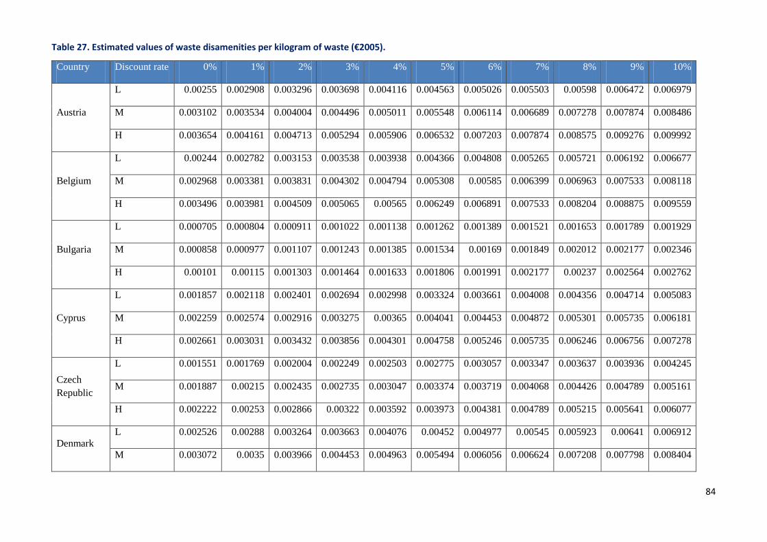
84
Table 27. Estimated values of waste disamenities per kilogram of waste (€2005).
Country Discount rate 0% 1% 2% 3% 4% 5% 6% 7% 8% 9% 10%
Austria
L 0.00255 0.002908 0.003296 0.003698 0.004116 0.004563 0.005026 0.005503 0.00598 0.006472 0.006979
M 0.003102 0.003534 0.004004 0.004496 0.005011 0.005548 0.006114 0.006689 0.007278 0.007874 0.008486
H 0.003654 0.004161 0.004713 0.005294 0.005906 0.006532 0.007203 0.007874 0.008575 0.009276 0.009992
Belgium
L 0.00244 0.002782 0.003153 0.003538 0.003938 0.004366 0.004808 0.005265 0.005721 0.006192 0.006677
M 0.002968 0.003381 0.003831 0.004302 0.004794 0.005308 0.00585 0.006399 0.006963 0.007533 0.008118
H 0.003496 0.003981 0.004509 0.005065 0.00565 0.006249 0.006891 0.007533 0.008204 0.008875 0.009559
Bulgaria
L 0.000705 0.000804 0.000911 0.001022 0.001138 0.001262 0.001389 0.001521 0.001653 0.001789 0.001929
M 0.000858 0.000977 0.001107 0.001243 0.001385 0.001534 0.00169 0.001849 0.002012 0.002177 0.002346
H 0.00101 0.00115 0.001303 0.001464 0.001633 0.001806 0.001991 0.002177 0.00237 0.002564 0.002762
Cyprus
L 0.001857 0.002118 0.002401 0.002694 0.002998 0.003324 0.003661 0.004008 0.004356 0.004714 0.005083
M 0.002259 0.002574 0.002916 0.003275 0.00365 0.004041 0.004453 0.004872 0.005301 0.005735 0.006181
H 0.002661 0.003031 0.003432 0.003856 0.004301 0.004758 0.005246 0.005735 0.006246 0.006756 0.007278
Czech Republic
L 0.001551 0.001769 0.002004 0.002249 0.002503 0.002775 0.003057 0.003347 0.003637 0.003936 0.004245
M 0.001887 0.00215 0.002435 0.002735 0.003047 0.003374 0.003719 0.004068 0.004426 0.004789 0.005161
H 0.002222 0.00253 0.002866 0.00322 0.003592 0.003973 0.004381 0.004789 0.005215 0.005641 0.006077
Denmark L 0.002526 0.00288 0.003264 0.003663 0.004076 0.00452 0.004977 0.00545 0.005923 0.00641 0.006912
M 0.003072 0.0035 0.003966 0.004453 0.004963 0.005494 0.006056 0.006624 0.007208 0.007798 0.008404

85
Country Discount rate 0% 1% 2% 3% 4% 5% 6% 7% 8% 9% 10%
H 0.003619 0.004121 0.004667 0.005243 0.005849 0.006469 0.007134 0.007798 0.008493 0.009187 0.009896
Estonia
L 0.001249 0.001424 0.001614 0.001811 0.002015 0.002234 0.002461 0.002694 0.002928 0.003169 0.003417
M 0.001519 0.00173 0.00196 0.002201 0.002453 0.002716 0.002993 0.003275 0.003563 0.003855 0.004154
H 0.001789 0.002037 0.002307 0.002592 0.002891 0.003198 0.003526 0.003855 0.004198 0.004541 0.004892
Finland
L 0.002331 0.002659 0.003013 0.003381 0.003763 0.004172 0.004595 0.005031 0.005467 0.005917 0.006381
M 0.002836 0.003231 0.003661 0.004111 0.004581 0.005072 0.00559 0.006115 0.006654 0.007199 0.007758
H 0.00334 0.003804 0.004308 0.00484 0.005399 0.005972 0.006585 0.007199 0.00784 0.008481 0.009135
France
L 0.002264 0.002582 0.002926 0.003284 0.003654 0.004051 0.004462 0.004886 0.005309 0.005746 0.006196
M 0.002754 0.003138 0.003555 0.003992 0.004449 0.004925 0.005428 0.005938 0.006461 0.006991 0.007534
H 0.003244 0.003694 0.004184 0.0047 0.005243 0.005799 0.006395 0.006991 0.007613 0.008235 0.008871
Germany
L 0.002389 0.002724 0.003087 0.003464 0.003855 0.004275 0.004708 0.005155 0.005602 0.006063 0.006538
M 0.002906 0.003311 0.003751 0.004212 0.004694 0.005196 0.005727 0.006265 0.006817 0.007376 0.007948
H 0.003422 0.003897 0.004414 0.004959 0.005532 0.006118 0.006747 0.007376 0.008032 0.008689 0.009359
Greece
L 0.001896 0.002162 0.002451 0.00275 0.003061 0.003393 0.003737 0.004092 0.004447 0.004813 0.00519
M 0.002307 0.002628 0.002977 0.003343 0.003726 0.004125 0.004547 0.004974 0.005412 0.005855 0.00631
H 0.002717 0.003094 0.003504 0.003937 0.004391 0.004857 0.005356 0.005855 0.006376 0.006897 0.00743
Hungary L 0.001291 0.001473 0.001669 0.001873 0.002084 0.002311 0.002545 0.002787 0.003028 0.003278 0.003534
M 0.001571 0.00179 0.002028 0.002277 0.002538 0.002809 0.003096 0.003387 0.003685 0.003988 0.004297

86
Country Discount rate 0% 1% 2% 3% 4% 5% 6% 7% 8% 9% 10%
H 0.00185 0.002107 0.002386 0.002681 0.002991 0.003308 0.003648 0.003988 0.004342 0.004697 0.00506
Ireland
L 0.002945 0.003358 0.003805 0.00427 0.004753 0.005269 0.005803 0.006354 0.006905 0.007473 0.008059
M 0.003582 0.004081 0.004623 0.005192 0.005786 0.006406 0.00706 0.007723 0.008403 0.009092 0.009798
H 0.004219 0.004804 0.005441 0.006113 0.006819 0.007542 0.008317 0.009092 0.009901 0.01071 0.011537
Italy
L 0.002139 0.00244 0.002765 0.003103 0.003453 0.003828 0.004216 0.004617 0.005017 0.00543 0.005855
M 0.002602 0.002965 0.003359 0.003772 0.004204 0.004654 0.00513 0.005611 0.006105 0.006606 0.007119
H 0.003065 0.003491 0.003954 0.004441 0.004954 0.00548 0.006043 0.006606 0.007194 0.007782 0.008383
Latvia
L 0.000993 0.001132 0.001283 0.00144 0.001603 0.001777 0.001957 0.002143 0.002329 0.00252 0.002718
M 0.001208 0.001376 0.001559 0.001751 0.001951 0.00216 0.002381 0.002605 0.002834 0.003066 0.003304
H 0.001423 0.00162 0.001835 0.002062 0.0023 0.002544 0.002805 0.003066 0.003339 0.003612 0.003891
Lithuania
L 0.001081 0.001233 0.001397 0.001568 0.001745 0.001934 0.00213 0.002333 0.002535 0.002743 0.002958
M 0.001315 0.001498 0.001697 0.001906 0.002124 0.002352 0.002592 0.002835 0.003085 0.003338 0.003597
H 0.001549 0.001764 0.001998 0.002244 0.002503 0.002769 0.003053 0.003338 0.003635 0.003932 0.004235
Netherlands
L 0.002673 0.003048 0.003454 0.003876 0.004314 0.004783 0.005267 0.005767 0.006268 0.006783 0.007315
M 0.003251 0.003704 0.004197 0.004712 0.005252 0.005814 0.006408 0.00701 0.007627 0.008253 0.008894
H 0.003829 0.004361 0.004939 0.005549 0.00619 0.006846 0.007549 0.008253 0.008987 0.009722 0.010472
Norway L 0.0036 0.004106 0.004653 0.005222 0.005811 0.006443 0.007096 0.007769 0.008443 0.009138 0.009854
M 0.004379 0.00499 0.005653 0.006348 0.007075 0.007833 0.008633 0.009443 0.010275 0.011117 0.01198

87
Country Discount rate 0% 1% 2% 3% 4% 5% 6% 7% 8% 9% 10%
H 0.005159 0.005874 0.006653 0.007475 0.008338 0.009222 0.01017 0.011117 0.012107 0.013096 0.014107
Poland
L 0.001048 0.001195 0.001355 0.00152 0.001692 0.001876 0.002066 0.002262 0.002458 0.00266 0.002869
M 0.001275 0.001453 0.001646 0.001848 0.00206 0.00228 0.002513 0.002749 0.002992 0.003237 0.003488
H 0.001502 0.00171 0.001937 0.002176 0.002428 0.002685 0.002961 0.003237 0.003525 0.003813 0.004107
Portugal
L 0.001571 0.001792 0.002031 0.002279 0.002536 0.002812 0.003097 0.003391 0.003685 0.003988 0.004301
M 0.001911 0.002178 0.002467 0.002771 0.003088 0.003418 0.003768 0.004121 0.004484 0.004852 0.005229
H 0.002251 0.002564 0.002904 0.003262 0.003639 0.004025 0.004438 0.004852 0.005284 0.005716 0.006157
Romania
L 0.000715 0.000816 0.000924 0.001037 0.001154 0.00128 0.001409 0.001543 0.001677 0.001815 0.001957
M 0.00087 0.000991 0.001123 0.001261 0.001405 0.001556 0.001715 0.001876 0.002041 0.002208 0.00238
H 0.001025 0.001167 0.001322 0.001485 0.001656 0.001832 0.00202 0.002208 0.002405 0.002601 0.002802
Slovakia
L 0.00123 0.001403 0.00159 0.001784 0.001985 0.002201 0.002424 0.002654 0.002885 0.003122 0.003367
M 0.001496 0.001705 0.001931 0.002169 0.002417 0.002676 0.002949 0.003226 0.003511 0.003798 0.004093
H 0.001762 0.002007 0.002273 0.002554 0.002849 0.003151 0.003475 0.003798 0.004136 0.004474 0.00482
Slovenia
L 0.001786 0.002037 0.002308 0.00259 0.002883 0.003196 0.00352 0.003854 0.004188 0.004533 0.004888
M 0.002172 0.002475 0.002804 0.003149 0.003509 0.003885 0.004282 0.004684 0.005097 0.005514 0.005943
H 0.002559 0.002914 0.0033 0.003708 0.004136 0.004574 0.005044 0.005514 0.006005 0.006496 0.006997
Spain L 0.002084 0.002377 0.002694 0.003023 0.003364 0.00373 0.004108 0.004498 0.004888 0.00529 0.005704
M 0.002535 0.002889 0.003273 0.003675 0.004095 0.004534 0.004997 0.005467 0.005948 0.006436 0.006935

88
Country Discount rate 0% 1% 2% 3% 4% 5% 6% 7% 8% 9% 10%
H 0.002986 0.003401 0.003852 0.004327 0.004827 0.005339 0.005887 0.006436 0.007008 0.007581 0.008166
Sweden
L 0.002458 0.002803 0.003177 0.003565 0.003968 0.004399 0.004844 0.005305 0.005765 0.006239 0.006728
M 0.00299 0.003407 0.00386 0.004334 0.00483 0.005348 0.005894 0.006447 0.007015 0.00759 0.00818
H 0.003522 0.004011 0.004543 0.005103 0.005693 0.006296 0.006943 0.00759 0.008266 0.008941 0.009631
United Kingdom
L 0.002489 0.002838 0.003217 0.00361 0.004017 0.004454 0.004905 0.005371 0.005836 0.006317 0.006812
M 0.003027 0.003449 0.003908 0.004388 0.00489 0.005414 0.005967 0.006528 0.007103 0.007685 0.008282
H 0.003566 0.004061 0.004599 0.005167 0.005764 0.006375 0.00703 0.007685 0.008369 0.009053 0.009752
89
Regarding incinerators, a few interesting primary studies have been found (see the studies described below), which could in principle be used for the value transfer using a similar methodology as for landfills. However, some of the key data related to the primary studies were impossible to localise, therefore, eventually the value transfer for incinerators was impossible to perform.
Value transfer for incinerators
Kiel and McClain (1995) measured the evolution and the consequential effects of public opposition to waste-to-energy incinerators on property values. The study was conducted near Boston, Massachusetts from January 1974 up to May 1992 on 2593 single family housing units. The incinerator was open for operation in the mid-1980s.
Description of the existing studies on incinerators
They had found that previous research had neglected to look at the profiles of change in social welfare, and whether this would have an impact in terms on under- / over- compensation of individual properties. While in the past, most studies had found a positive relationship between property prices and distance to the facility, no attempt had been made to look at the house price adjustments over an extended period of time. As a result, they divided their research into five stages of risk:
1) Pre-rumour of facility on the neighbouring area (1974-1978);
2) Fully established rumour, through the media, prior to construction (1979-1980);
3) Construction of the facility (1981-1984);
4) Operation of the facility, and full awareness of health and safety risks (1985-1988); and
5) Ongoing operation – similar to stage one, except with the waste facility in place (1989-1992).
Stage 5 provides a reference of the differences between the conditions prior to any mention of the waste facility in the area. The movement of house prices over time is measured using hedonic regression models. The outcome indicates that the siting of the facility is perceived as a disamenity, the equilibrium price of a house near a facility is lower, after adjusting for inflation, than it was in the first stage. Otherwise, it would be regarded as having a benign impact. The results showed that the impacts of siting of the incinerator were felt for seven years after waste operations started. They concluded that the adjustment of house prices to a waste facility is more complicated and prolonged over a longer time span than previously thought. As a result this study is useful to advocate that measures for valuing the effects of external effects from waste disamenities should reflect change over the lifespan of the disamenity to reflect the true costs to society.
5 Externalities not included in the EFORWOOD project
5.1 Biodiversity
Biodiversity is related to forest conservation or restoration of national parks and reserves, by managing existing habitats at the expense of commercial timber production, and encourage

90
the diversion away from monocultures, and by preserving or reintroducing rare and endemic species. Hence, it is a very broad term that is applicable at the genetic, species and habitat level.
In the set of indicators, biodiversity refers to areas of protected forests, ecosystem functions such as soil and water, tree species composition, carbon in standing and lying deadwood, and landscape patterns. Biodiversity is sub-divided for the ecosystem level (indicator: area of selected key ecosystems) and at the species level (indicator: abundance of selected key species). Biodiversity may not respond so obviously to changes in material flows along a selected FWC, but it can be linked to the area of forest under a certain management regime.
Five research objectives, as follows, were proposed for the biodiversity indicator in terms of the changes brought about from the scenarios (D.1.1.1, 2006):
1) Is there a reduction in the biological diversity in terms of the number of species, the variety and/or races in an area, or is conservation promoted, leading to an increase in diversity?
2) Is there an impact on protected or endangered species or their habitats, or ecologically sensitive areas?
3) Is there landscape fragmentation, or is there an impact on migration route, ecological corridors or buffer zones?
4) Are the scenic values of protected landscapes affected by scenario changes?
5) Is there a change in status of species in terms of either becoming threatened or protected?
In terms of the CBA, there remain several challenges of how to put a value on biodiversity as such (Nunes and van den Bergh 2001). If one was to take look at the level of biodiversity resources, there would need to be a distinction between whether this consists of diversity or stock, the latter would imply that diversity is low while biomass would be high. As a result of a lack of valuation studies in this field that focus on more abstract aggregates of the concept (Christie et al 2006), there remains a gap in the understanding of how far individual’s value biodiversity (attempts have been made in the UK by ERM, 1996, and in the tropics by Pagiola et al., 2002). There are numerous valuation studies that have addressed individual’s WTP for what can be considered biodiversity, e.g. habitats or sites (Jacobsen et al 2008; Jacobsen and Thorsen 2010) or specific species (White et al 1997; Jakobsson and Dragun 2001; Tisdell et al 2005; Hanley et al 2003), but these are best regarded as components of diversity, and not biodiversity as such. Defra (2003b) states that market valuation is consistent with the ‘homogenisation’ of forests and other ecosystems, and do not take into consideration ‘multi-purpose’ forests. Due to the level of uncertainty, biodiversity has therefore not been included in the CBA of the EFORWOOD project.
5.2 Landscape beauty
Due to similar reasons as those for biodiversity, markets are unlikely to capture the benefits of forests in terms of landscape beauty, as result of ‘non-use’ values having no behavioural trail. Defra (2003b) did suggest that capitalising landscape beauty would be possible through special funds based on donations, to secure the benefits from landscape beauty. However,

91
they also state that the free rider problem would be significant (i.e. people enjoying the benefits of a good without paying for them). As a result, landscape beauty was not seen as a viable component of the CBA for the EFORWOOD project.
5.3 Soil pollution
Soil pollution represents an important externality from different FWC processes. Unfortunately, there is no indicator on the physical amount of such pollution to which a monetary estimate could be potentially attached. Therefore, in the context of EFORWOOD, soil pollution is not included in the valuation study. Nevertheless, for waste disposal disamenities, the monetary estimate considers the possible external effect of soil pollution (see Section 4.6.5.4).
5.4 Noise
Noise is a side effect of many processes in the FWC (e.g. harvesting, transport, wood processing). It does not only affect the working conditions of the employees (which in principle should be reflected in labour costs), but may also affect the wellbeing of agents not involved in the production process. Therefore it is clearly an external effect of the FWC. Noise is considered an externality in the cases where third parties are affected, that is, causing noise in remote uninhabited areas does not count as an externality.
The welfare economic costs of noise may be obtained from relevant hedonic studies, considering the exact context in which this impact and potential externality occurs. In the framework of the EFORWOOD project, however, there is no indicator measuring the physical quantity of noise (in dB) from different processes, therefore, in general, the valuation of noise has been considered as not feasible in the project. It must be mentioned, nevertheless, that noise forms part of waste related disamenities, and therefore, the external effect of noise is included in the monetary estimate of waste disamenities (see Section 4.6.5.4).
5.5 Odour
Just as noise, unpleasant smell can be one of the negative side effects of the production processes of the FWC (e.g. pulp and paper industry). The externality is present when agents not involved in the production process are affected. An open question here is how it can be measured in physical terms, and valued in monetary terms. There exist hedonic studies of the welfare costs of living close to very smelly industries, e.g. large Danish pig industries. Nevertheless, and similarly to noise, it is necessary to identify the exact context in which this impact and potential externality occurs. In the context of EFORWOOD, there is no indicator measuring the physical amount of odour produced in different processes, therefore, the valuation of odour has been considered as not feasible in the project. At the same time, the external effect of odour, similarly to that of noise, is included in the monetary estimate of waste disamenities (see Section 4.6.5.4).
5.6 Occupational accidents
In the standard cost-benefit analysis, it is frequently assumed that the safety and health risks of a certain job are known to the employees before they accept the job, therefore, it is considered that when an employee accepts the job, he or she is compensated by a higher

92
salary or increased non-salary benefits. This means that the increased risk of occupational accidents is not a real externality, as it not only has a market value, but is also transacted through labour markets. (e.g. Viscusi and Aldy, 2003). Therefore, it is not values separately for the purposes of the cost-benefit analysis.
5.7 Erosion
As a result of a lack of data on forest soil conditions for the main timber producing areas of Europe, it was deemed unfeasible to provide estimates of the costs of soil erosion by processes in the FWCs.
5.8 Employment creation
The measures of change in welfare, when new jobs are created, is generally already incorporated in and valuated by other economic indicators. There is, however, the issue that many policy makers adhere to particular values when creating new jobs in a certain region (e.g. less developed rural areas), and theoretically this could be captured in economic terms too. Nevertheless, as the scope of the cost-benefit analysis in EFORWOOD is limited to partial equilibrium analysis, the social aspect of employment creation is not valued, but should rather be considered within the multi-criteria analysis module (MCA).
6 Summary and conclusions The objective of the present document was to summarise the work on the monetary valuation of environmental and social externalities in the WP1.5 within the EFORWOOD project. The monetary estimates presented in this document form the core of the cost-benefit analysis implemented in the TOSIA-E software package developed during the project. The guidelines to incorporate these values into the cost-benefit analysis within TOSIA-E are presented in Annex IV.
The overall method chosen in EFORWOOD for this task is that of unit value transfer. No primary valuation studies were planned or have been undertaken in EFORWOOD. When possible and relevant, adjustments to unit values have been adopted. The transfer unit depends in all cases on the actual externality valued (see chapter 4). We undertook a spatial transfer adjustment for several externalities, when relevant. For this we used variation in wealth and income (as captured in GDP/capita) also at the intra-national level, and for the international transfer, we used purchasing power parity corrected adjusted measures of these along with the related exchange rates (see Annex II). Across time, we apply assumptions on the growth in wealth and income (GDP/capita) and on the link between this measure and the valuation (see Annex I).
This approach allowed us to assign value estimates to several of the externalities related to the EFORWOOD indicator set for sustainability assessment. These included:
• Recreation
• Non-greenhouse gas emissions
• GHG emissions and carbon stock in FWCs
• Water pollution

93
• Transport externalities
• Waste externalities
The following externalities were not covered, with monetary values at least, in the EFORWOOD project:
• Biodiversity
• Landscape beauty
• Soil pollution
• Noise
• Odour
• Occupational accidents
• Erosion
Most of the monetary estimates present the values of the marginal external costs (and benefits) of a given externality, with the exception of waste disamenity costs which are average values. Due to the fact that all the estimates have been obtained using benefit transfer method, it should be kept in mind that the reliability of these estimates is contingent on the quality of the primary valuation studies. In most of the cases, the values are fairly robust (e.g. recreation, air pollution, accident costs), while in other the limited number of relevant primary valuation studies may make them weaker. This is especially the case of waste disamenities, in which the limited number of relevant and up to date primary studies sheds shadow on the obtained estimates. In addition, it has to be mentioned that some external cost estimates have been obtained in very specific contexts (e.g. water pollution estimates are mainly based on the studies in the field of agriculture), which may limit their applicability to the forest sector in general. These issues represent some of the most important challenges for the future work on the estimates of both positive and negative externalities related to forest-wood chain activities.
Another issue worth mentioning is the fact that the estimates for different externalities have been obtained using different valuation techniques. Some of them rely on contingent valuation methods (e.g. recreation), other on hedonic studies (e.g. waste disamenities), while other values are based on abatement cost methods (e.g. GHG and water pollution) or on market price methods (e.g. accident costs). This is due to the fact that there does not exist a unique approach to value all the aspects of any given externality. The reliance on different valuation techniques (and hence, different notions of value) can give rise to a certain inconsistency of estimates, however, this issue can hardly be overcome. In addition, it has to be acknowledged that different valuation methods present different range of estimates: market price methods and avoidance cost methods typically represent the lower range estimates, while stated preference methods eliciting WTA measures typically represent the higher range estimates of value. In the EFORWOOD project, this issue has been handled by introducing minimum, maximum and average estimates of values. In some cases the differences between the minimum and the maximum values are rather substantial which may have important implications for the final results of the CBA analysis especially when the physical quantities of related external effects are significant. Nevertheless, we consider that giving a single

94
estimate for any given externality would give a rather distorted picture of the possible monetary values. One has to keep in mind that the uncertainties in the valuation of many externalities (e.g. especially in the field of climate change, air and water pollution, etc.) are related not only to the choice and subsequent limitations of different valuation methods, but also to the uncertainties in predicting the actual physical impacts triggered by these externalities. Therefore, the use of minimum, maximum and average value estimates is intended to give a fuller picture on the range of “true” externality values.
7 References AEA Technology (CAFE CBA) (2005): Service contract for carrying out cost-benefit
analysis (CBA) of air quality related issues, in particular in the Clean Air For Europe (CAFE) programme, Final Methodology Paper, Vol. 1 (4), EC DG Environment.
André García F.J. and Cerdá Tena (2001): Landfilling, set-up costs and optimal capacity, Centro de Estudios Andaluces.
Arrow K. and Fischer A. (1974): Environmental preservation, uncertainty and irreversibility. Quarterly Journal of Economics, Vol. 88, pp. 312-319.
Atkins J.P. and Burdon D. (2006): An initial economic evaluation of water quality improvement in the Randers Fjord, Denmark. Marine Pollution Bulletin (2006) 53, pp. 195-204.
Ayres R.U. and Walter J. (1991): The greenhouse effect: Damages, costs and abatement. Environmental and Resource Economics, Vol. 1, pp. 237-270.
Bateman I.J., Jones A.P., Nishikawa N. and Brouwer R (2000): Benefits Transfer in Theory and Practice: A Review. CSERGE Working Paper GEC 2000-25.
Berntsen J., Petersen B.M., Jacobsen B.H., Olesen J.E. and Hutchings N.J. (2003): Evaluating nitrogen taxation scenarios using the dynamic whole farm simulation model FASSET. Agricultural Systems (2003) 76, pp. 817-839.
Bickel P. and Friedrich R. (2001): Estimating environmental costs using the Impact Pathway Approach, Institut für Energiewirtschaft und Rationelle Energieanwendung, Universität Stuttgart, Germany.
Blok K., de Jager D. and Hendriks C. (2001): Economic evaluation of sectoral emission reduction objectives for climate change - Summary report for policy makers, ECOFYS Energy and Environment, AEA Technology, National technical university of Athens, Utrecht, March 2001. (http://europa.eu.int/comm/environment/enveco/climate_change/sectoral_objectives.htm)
Bonnieux F. and Desaigues B. (1998): Économie et politique de l’environnement. Dalloz, Paris.
Bonnieux F. and Rainelli P., (2003): La technique des transferts dans l'évaluation des biens non-marchands: une application. Revue d'Économie Régionale et Urbaine 2. INRA – Économie.

95
Bouvier R.A, Halstead J.M, Conway K.S. and Manalo A.B (2000): “The effect of landfills on rural residential property values”. Journal of Regional Analysis and Policy, Vol. 30 (2), pp. 23-37.
Boyle M.A and Kiel K.A. (2001): A survey of house price hedonic studies of the impact of environmental externalities. Journal of Real Estate Literature, Vol.9, pp. 117-144.
Brady, M. (2003): The relative cost-efficiency of arable nitrogen management in Sweden. Ecological Economics (2003) 47, pp. 53-70.
Brisson I. and Pearce D. (1995): Benefits transfer for disamenity from waste disposal, CSERGE Working Paper WM95-06, University College London, and University of East Anglia.
Byström O. (1998): The nitrogen abatement cost in wetlands. Ecological Economics (1998) 26, pp. 321-331.
Byström O. (2000): The replacement value of wetlands in Sweden. Environmental and Resource Economics (2000) 16, pp. 347-362.
Byström O., Andersson H. and Gren I.M. (2000): Economic criteria for using wetlands as nitrogen sinks under uncertainty. Special issue: The values of wetlands: Landscape and institutional perspectives. Ecological Economics (2000) 35, pp. 35-45.
Capros P. and Mantzos L. (2000): Kyoto and technology at the European Union: costs of emission reduction under flexibility mechanisms and technology progress. Int. J. Global Energy Issues, 14, p.169-183.
CE Delft (2004): The price of transport: overview of the social costs of transport (eds. Vermeulen J.P.L., Boon B.H., van Essen H.P., den Boer L.C., Dings J.M.W., Bruinsma F.R., Koetse M.J.)
Chèze B. (2008): Economic valuation of environmental damages of waste sites. What can meta-analysis tell us about variations in amenity costs estimates? AFESE
Christie, M., N. Hanley, J. Warren, K. Murphy, R. Wright and T. Hyde (2006), ‘Valuing diversity of biodiversity’. Ecological Economics, vol. 58, 304-317.
Cline W.R. (1992): Optimal carbon emissions over time: experiments with the Nordhaus DICE Model, Washington D.C.: Institute for International Economics.
Cline W.R. (1993): The Economics of Climate Change, Institute for International Economics, Washington D.C.
COST 313 (1994): COST 313 Socio-economic costs of road accidents. Final report. Office for Official Publications of the European Communities. Luxemburg.
COWI (2000): A study on the economic valuation of environmental externalities from landfill disposal and incineration of waste, European Commission DG Environment.
Dames and Moore (1999): The Implications for the UK of an International emissions Trading Scheme. London: Department of the Environment, Transport and Regions.
Davidson M.D., Hof A.F. and Potjer B. (2002): Update schaduwprijzen. Financiële waardeing van milieu-emissies op basis van Nederlandse overheidsdoelen [Update

96
shadow prices. Financial valutaion of environmental emissions based upon policy targets in the Netherlands], Delft: CE Environmental Research and Consultancy.
Department of Environment (1993): Externalities from landfill and incineration, London, HMSO.
Defra (2002): Estimating the social cost of carbon emissions (Eds. Clarkson R. and Deyes K.), Government Economic Service (UK GES) Working Paper 140.
Defra (2003a): A study to estimate the disamenity costs of landfill in Great Britain, Cambridge Econometrics, EFTEC and WRc. Available for download from the Defra Internet site (http://www.defra.gov.uk/environment/waste/topics/landfill-dir/disamenity.htm).
Defra (2003b): Economic Analysis Forestry Policy in England (eds. CJC Consulting with Pearce D. and Willis K.).
Defra (2007): The Social Cost of Carbon and the Shadow Price of Carbon: What they are, and how to use them in economic appraisal in the UK (eds. R. Price, S. Thornton, and S. Nelson). Economics Group Defra, London, UK.
Dijkgraaf E and Vollebergh H.R.J. (2003): Burn or bury? A social cost comparison of final waste disposal methods, Fondazione Eni Enrico Mattei Note di Lavoro Series. Available for download from the FEEM website (http://www.feem.it/web/activ/_wp.html).
DLR (2006): Externe Kosten der Stromerzeugung aus erneuerbaren Energien im Vergleich zur Stromerzeugung aus fossilen Energieträgern Stuttgart/Karlsruhe : Deutsches Zentrum für Luft- und Raumfahrt (DLR)/ Fraunhofer Institut für System- und Innovationsforschung (ISI) (eds. Krewitt W. and Schlomann B.).
Earnhart, D. (2001): ‘Combining Revealed and Stated Preference Methods to Value EnvironmentalAmenities at Residential Locations’. Land Economics, Feb, Vol. 77(1), pp 12–29.
EC (1996): Cost-benefit analysis of the different municipal solid waste management systems: objectives and instruments for the year 2000, Final report to the European Commission, Luxembourg: Office for Official Publications of the European Communities, (eds. Coopers and Lybrand, CSERGE and EFTEC).
ECOTEC (2000): Beyond the bin: the economics of waste management options, ECOTEC for Friends of the Earth, UK Waste and Waste Watch.
EEA (2000): COPERT II Computer programme to calculate emissions from road transport: Methodology and emission factors (version 2.1) (eds. Ntziachristos L. and Samaras Z.).
EFORWOOD (2008): PD.0.0.16 Manual for data collection for regional and European cases. Working document for Task Force (ed. Berg, S.)
EFORWOOD (2006): D. 1.1.1 Draft FWC indicator set: Detailed review of existing sustainability indicator concepts and sustainability indicator sets of relevance for the

97
FWC, review of potential indicators for selection and their assessment (eds. Rametsteiner E, Pülzl H., and Puustjärvi E.).
EFORWOOD (2006): P.D. 1.5.1 A guideline for selecting and defining externalities in Modules 2-5, including data format considerations (eds. Mavsar, R., Prokofieva I., Giergiczny M., Jellesmark Thorsen B. and Vedel S.E.)
EFORWOOD (2007): P.D. 2.0.5 Updated report on the forest-based case study “Scandinavian regional case” (eds. Valinger E. et al.).
EFORWOOD (2007): P.D. 3.0.3 Definition of case study “Baden-Württemberg” – Status report, (eds. Brüchert F. et al.)
EFORWOOD (2008): D 1.4.7 Reference futures and scenarios for the European FWC (eds. Arets E. Palosuo T., Moiseev A., Nabuurs G-J, Slimani D., Olsmat C., Laurijssen J., Mason B., McGowan D., and Vötter D.).
EFORWOOD (2009): D. 2.2.2 Synthesis report on impact of forest management on environmental services (eds. Raulund-Rasmussen K. and Hansen K.).
EFORWOOD (2009): P.D. 3.3.4 Data collection of transport processes to ToSIA at case study and EU level (eds. FCBA).
EFORWOOD (2009): P.D. 3.3.6 Stratified partial model on transport (eds. FCBA).
Ekeland, I., Heckman, J.J. and L. Nesheim (2004): Identification and Estimation in Hedonic Models. Journal of Political Economy, vol. 112, s60-s109.
Elliott, S.J., S.M. Taylor, C. Hampson, J. Dunn, J. Eyles, S.Walter and D. Streiner (1997): “It’s Not Because You Like it any Better...”: Residents’ Reappraisal of a Landfill Site. Journal of Environmental Psychology, Vol.17, pp 229–41.
Elofsson K. (2006): Cost-effective control of interdependent water pollutants. Environmental Management, Vol. 37 (1), pp 54-68, 2006.
ERM, Environmental Resources Management (1996): Valuing management for biodiversity in British forests, Report to the UK Forestry Commission.
Eyre N., Downing T.E, Hoekstra R. and Rennings K. (1999): Externalities of Energy, Vol. 8: Global Warming, Luxembourg: Office for Official Publications of the European Communities, pp.1-50.
EXIOPOL (2008): Report documenting the results of the meta-data analysis linking the monetary values with the physical characteristics of forests (Eds. Giergiczny M., Mavsar R. and Wenchao Z.). EXIOPOL: A new environmental accounting framework using externality data and input-output tools for policy analysis. Priority 6.3 Global Change in Ecosystems in the 6th EU framework programme. European Commission.
ExternE, Externalities of energy (2005): Methodology 2005 Update (Eds. Bickel P. and Friedrich R.) DG Research Sustainable Energy Systems, Institut für Energiewirtschaft und Rationelle Energiernawendung – IER, Universität Stuttgart, Germany.
Fankhauser S. (1994): Evaluating the social costs of Greenhouse Gas Emissions, CSERGE Working Paper GEC 94-01, University College London, and University of East Anglia.

98
FAO (2004): Trends and current status of the contribution of the forestry sector to national economies. FAO Working Paper FSFM/ACC/07. Rome. Available for download from the FAO website (http://www.fao.org/docrep/007/ad493e/ad493e00.htm).
Fisher, A. C. (2000): Investment under uncertainty and option value in environmental economics, Resource and Energy Economics 22, 197-204.
Fisher, A.C., and Hanemann, W.M. (1987): Quasi-option value: some misconceptions dispelled, Journal of Environmental Economics and Management 14, 183-90.
Friedrich R. and Bickel P. (2001): Environmental external costs of transport. Stuttgart: IER, university of Stuttgart.
Garrod G. and Willis K. (1998): Estimating lost amenity due to landfill waste disposal. Resources, Conservation and Recycling, Vol.22 (1-2), pp. 82-95.
Garrod, G. and Willis, K.G. (1999), Economic Valuation of the environment: methods and case studies. Cheltenham, Edward Elgar.
GRACE (2006) Generalisation of Research on Accounts and Cost Estimation: Environmental costs in Sensitive areas (eds. Lied C., Suter S. and Bickel P.). ITS University of Leeds.
Gren I.M. (1999): Value of land as a pollutant sink for international waters. Ecological Economics (1999) 30, pp.419-431.
Gren I.M., Elofsson K. and Jannke P. (1997a). Cost-effective nutrient reduction to the Baltic Sea. Environmental and Resource Economics (1997) 10, pp. 341-362.
Gren I.M., Söderqvist T. and Wulff F., (1997b): Nutrient reductions to the Baltic Sea: Ecology, costs and benefits. Journal of Environmental Management (1997) 51, pp. 123-143.
Groothius P.A. (1994): Locating hazardous waste facilities: The influence of NIMBY beliefs. The American Journal of Economics and Sociology, Vol. 53 (3), pp. 335-347.
Hanley, N., D. Macmillan, I. Patterson and R. E. Wright (2003), ‘Economics and the design of nature conservation policy: a case study of wild goose conservation in Scotland using choice experiments’, Animal Conservation, vol. 6, 123-129.
HEATCO (2006): Developing Harmonised European Approaches for Transport Costing and Project Assessment, Deliverable 5: Proposal for Harmonised Guidelines (ed. Bickel P. et al.), Stuttgart: IER, Germany.
Helin J., Laukkanen M. and Koikkalainen K. (2006): Abatement costs for agricultural nitrogen and phosphorous loads: a case study of crop farming in south-western Finland. Agricultural and Food Science, Vol. 15, pp. 351-374.
Henscher D.A, Rose J.M. and Green W.H. (2005): Applied choice analysis: A Primer. Cambridge University Press.
Holland M.R and Forster D (1999): Externalities of Energy, ExternE Project, Report Number 7, Methodology: Update 1998. EC Commission DG Research.

99
Holland M and Watkiss P (2002): Benefits Table database: Estimates of the marginal external costs of air pollution in Europe, BeTa Version E1.02a, Netcen, AEA Technology, EC DG Environment.
Huhtala A., Marklund P.O. (2008): Stringency of environmental targets in an animal agriculture: shedding light on policy with shadow prices. European Review of Agricultural Economics, Vol. 35 (2) (2008), pp. 193-217.
IMPACT (2008): Handbook on estimation of external costs in the transport sector, Version 1.1, (eds Mailbach M. et al.) CE Delft, European Commission DG TREN.
INFRAS (2004): Handbook emission factors for road transport (HBEFA 2.1) (ed. Keller M.). INFRAS Berlin/Berne/Vienna: German Umweltbundesamt; Swiss Agency for the Environment, Forests and Lansdcape 8SAEFL), Austrian Umweltbundesamt, Federal Ministry of Agriculture, Forestry, Environment and Water Management, Austrian Ministry of Transport, Innovation and Technology.
INFRAS/IWW (2000) External Costs of Transport: Accident, Environmental and Congestion Costs of Transport in Western Europe. Karlsruhe/Zürich/Paris: the International Union of Railways (UIC).
INFRAS/IWW (2004): External costs of transport: update study (eds. Scheyer C., Maibach M., Rothengatter W., Doll C., Schneider C., Schmedding D.). Karlsruhe/Zürich/Paris: the International Union of Railways (UIC).
IPCC (1996): Climate Change 1995: economic and social dimensions of climate change, Contribution of WGIII to the Second Assessment Report of the Intergovernmental Panel on Climate Change, CUP.
IPCC (2000): Special report emissions scenarios: Summary for policy makers. A special report of IPCC Working Group II.
IPCC Guidelines for National Greenhouse Gas Inventories AFOLU (2006). Available for download from the IPCC website (http://www.ipcc-nggip.iges.or.jp/public/2006gl/vol4.html).
IPCC (2007) Fourth Assessment Report of the IPCC. NY, Cambridge University Press.
Jacobsen B.H. (2002): Reducing nitrogen leaching in Denmark and the Netherlands – Administrative regulation costs. Poster Paper for the Xth Conference in Zaragoza, 2002.
Jacobsen B.H., Abildtrup J., Jensen J.D., Hasler B. (2005): Costs of reducing nutrient losses in Denmark – analyses of different regulation systems and cost effective measures. Poster paper for presentation at the XI Congress of the EAAE, Copenhagen, Denmark, 2005.
Jacobsen J.B., Boiesen J.H., Thorsen B.J. and N. Strange (2008): What’s in a Name? The use of Quantitative Measures vs. ’Iconised’ Species when Valuing Biodiversity. Environment and Resource Economics, vol. 39, 249-263

100
Jacobsen J.B. and B.J. Thorsen (2010): Where to put a national park and what to put in it? An a priori study of the willingness-to-pay for national parks. Forthcoming in Ecological Economics
Jakobsson, K. M. and A. K. Dragun (2001), ‘The Worth of a Possum: Valuing Species with the Contingent Valuation Method’, Environmental and Resource Economics, vol. 19, 211-227.
Johansson-Stenman O, and Svedsäter H (2008) Measuring Hypothetical Bias in Choice Experiments: The Importance of Cognitive Consistency. Topics in Economic Analysis and Policy, vol. 8, 1-8
Kampas A., White B. (2004): Administrative cost and instrument choice for stochastic non-point source pollutants. Environmental and Resource Economics(2004), 27, pp. 109-133.
Kiel and McClain (1995): House prices during siting decision stages: the case of an incinerator from rumor through operation. Journal of Environmental Economics and Management, Vol. 28, pp. 241-255.
Laukkanen M., Huhtala A. (2008): Optimal management of a eutrophied coastal ecosystem: Balancing agricultural and municipal abatement measures. Environmental Resource Economics (2008) 39, pp. 139-159.
Le Goffe P, (1995): The benefits of improvements in coastal water quality: a contingent approach. Journal of Environmental Management (1995) 45, pp 305-317.
Lindhjem H. and Stale N. (2007): How reliable are meta-analyses for International Benefit Transfers. Ecological Economics 66 (2-3), pp. 425-435.
Lim J.S. and Missios P. (2007): Does size really matter? Landfill scale impacts on property values. Applied Economics Letters, Vol. 14(10), pp. 719-723.
List JA Sinha P, Taylor MH (2006): Using Choice Experiments to Value Non-Market Goods and Services: Evidence from Field Experiments. Adv Econ Anal Pol 6:1-37
Lousteau D. (2001): CARBOFOR project: Carbon sequestration in large forest ecosystems in France. Quantification, spacialization and impact of various climatic and management scenarios. Management and Impacts of Global Change Programme GICC, CRP, INRA.
McCluskey J.J. and Rausser G.C. (2001): Hazardous waste sites and housing appreciation rates. Journal of Environmental Economics and Management 45, pp.166-176.
Maddison D. (1994): Economics and the environment: The shadow price of greenhouse gases and aerosols, Surrey Energy Economics Discussion Papers, SEEDS 76, University of Surrey.
Maibach M, Schreyer C, Sutter D, van Essen H.P., Boon B.H.m Smokers R., Schroten A. Doll C., Pawlowska B, and Bak M. (2008): Handbook on estimation of external costs in the transport sector, Produced within the study Internalisation Measures and Policies for All external Cost of Transport (IMPACT), CE Delft.

101
Mas-Colell A., Whinston M.D. and Green J.R. (1995): Microeconomic theory. Oxford University Press.
Mavsar R. (2008) Report documenting the results of the meta-analysis linking the monetary values with the physical characteristics of forests. EXIOPOL: A New Environmental Accounting Framework using Externality data and Input-Output Tools for Policy Analysis.
Mazzanti M. and Zoboli R. (2008): Waste generation, incineration and landfill diversion. De-coupling trends, socio-economic drivers and policy effectiveness in the EU, The Fondazione Eni Enrico Mattei Note di Lavoro Series. Available for download from the FEEM website (http://www.feem.it/Feem/Pub/Publications/WPapers/default.htm).
MCPFE (2007): State of Europe’s Forests 2007, the MCPFE report on sustainable forest management in Europe. Ministerial Conference on the Protection of Forests in Europe, Liaison Unit Warsaw.
Mensink, P. and T. Requate (2005) The Dixit-Pindyck and the Arrow-Fisher-Hanemann-Henry option values are not equivalent: a note on Fisher (2000), Resource and Energy Economics 27, 83-88.
Merlo M. and Croitoru L. (2005): Valuing Mediterranean forests: Towards total economic value. CABI Publishing.
Methodex D6 (2007): Methods and data on environmental and health externalities: harmonising and sharing of operational estimates, Deliverable 6, Report on Transfer Techniques. Available for download from the Methodex website (http://www.methodex.org/ReportonTransferTechniques.pdf).
Methodex D12 (2007): methods and data on environmental and health externalities: harmonising and sharing of operational estimates, Deliverable 12a, Final Technical Report: Methods.
Mitchell R.C, Carson R.T. (1989): Using surveys to value public goods: the contingent valuation method. Resources for the Future, Washington, D.C.
Münier B., Birr-Pedersen K., and Schou J.S. (2004): Combined ecological and economic modelling in agricultural land use scenarios. Ecological Modelling 174 (2004), pp. 5-18.
Navrud S. (2004): Value transfer and environmental policy. Chapter 5 (pp. 189-217) in Tietenberg T. And Folmer H. (eds) (2004): The international yearbook of environmental and resource economics 2004/2005. A survey of current issues. Edward Elgar Publishing, Cheltenham, UK and Northampton, MA, USA.
Navrud, S. (2005), Practical tools for value transfer in Denmark – guidelines and an example. Final report to Danish Environmental Protection Agency. Copenhagen. December 18, 2005.
Navrud S. and Brouwer R. (2007): Good practice guidelines in benefit transfer of forest externalities. COST Action E45, European Forest Externalities (EUROFOREX).

102
Navrud S. and Ready R. (eds) (2007): Environmental value transfer: Issues and methods. Springer Verlag.
Nelson A.C., Genereux J. and Genereux M. (1997): Price effects of landfills on different house value strata. Journal of Urban Planning and Development, 123(3), pp. 59-67.
Nordhaus W.D. (1991): To slow or not to slow: the economics of greenhouse effect. Economic Journal, Vol. 101 (407), pp.920-937.
Nordhaus W.D. (1992): An optimal transition path for controlling greenhouse gases, Science, Vol. 258, pp. 1315-1319.b
Nordhaus W.D. (1994): Managing the Global Commons: the Economics of Climate Change, MIT Press, Cambridge, Mass.
Nordhaus W.D. and Boyer J.G. (2000): Warming the world: Economic models of global warming, Cambridge: The MIT Press.
Nunes, P. A. L. D. and J. C. J. M. van den Bergh (2001), ’Economic valuation of biodiversity: sense or nonsense?’ Ecological Economics, vol. 39, 203-222.
Nunneri C., Windhorst W., Turner R.K., and Lenhart H. (2007): Nutrient emissions reduction scenarios in the North Sea: An abatement cost and ecosystem integrity analysis. Ecological Indicators, 7 (2007), pp. 776-792.
OECD (1992): Project and Policy Appraisal: Integrating Economics and Environment (eds. Pearce D., Whittington D., Georgiou S., and James D.).
OECD (2004): Addressing the economics of waste, OECD Publishing, Paris, France, 197p.
Pagiola S., Bishop J. and Landell-Mills N. (2002): Selling forest environmental services: market-based mechanisms for conservation and development, London: Earthscan.
Pearce D.W. (2003): The role of “property rights” in determining economic values for environmental costs and benefits. Report to the UK Environmental Agency, Bristol, Environmental Agency.
Pearce D. and Moran D. (1994): The Economic value of biological diversity. Earthscan.
Pearce D.W (2002): The Social Cost of Carbon and its Policy Implications, Economics and CSERGE, University College London and Environmental Science and Technology, Imperial College London.
Pearce D, Atkinson G. and Mourato S. (2006): Cost-benefit analysis and the environment: Recent developments: The Stages of a Practical cost-benefit analysis. OECD Publishing, Paris.
Peck S. and Teisberg T. (1993): Global Warming uncertainties and the value of information: an analysis using CETA. Resource and Energy Economics, Vol. 15 (1), pp. 71-97.
PETS (2000) Pricing European Transports Systems (PETS), Final Report (eds. Nash, C. et al.). ITS University of Leeds.
Plambeck E. and Hope C. (1996): PAGE95: an updated valuation of the impacts of global waming.Energy Policy, Vol. 24 (9), pp. 783-793.

103
Powell J.C. and Brisson I. (1994): The assessment of social costs and benefits of waste disposal, CSERGE Working Paper WM 94-06, Univeristy of East Anglia and University College London.
Rabl A. and Spadaro J.V. (2000): Health Costs of Automobile Pollution, Revue Française d’Allergologie et d’Immunologie Clinique, Vol.40 (1), pp. 55-59.
Ready R. (2005): Do Landfills always depress nearby property values? Rural Development Paper Nº27, Depat. Of Agricultural Economics and Rural Sociology, Pennsylvania State University, USA.
Ready R.C., Navrud S., Day B., Dubourg R., Machado F., Mourato S., Spanninks F. and Rodriguez M.X.V. (2004): Benefit Transfer in Europe. How reliable are transfers between countries? Environmental and Resource Economics 29, 67-82.
RECORDIT (2000): Real Cost Reduction of Door-to-Door Intermodal Transport (RECORDIT) Deliverable 1: Accounting Framework (eds. Weinreich S. (ZEW) et al.). Mannheim: ZEW Center for European Economic Research.
RECORDIT (2001): Real Cost Reduction of Door-to-Door Intermodal Transport (RECORDIT) Deliverable 4: External cost calculation for selected corridors (eds. Schmid, S.A. et al.). Stuttgart: IER/university of Stuttgart.
Reichert A., Small M., and Mohanty S. (1992): The impact of landfills on residential property values. Journal of Real Estate Research, Vol 7(3), pp. 297-314.
Rinaud J.D., Arnal C., Blanchin R., Elsass P., Meilhac A. and Loubier S. (2005): Assessing the cost of groundwater pollution: the case of diffuse agricultural pollution in the Upper Rhine walley aquifer. Water Science andTechnology, Vol. 55(9), pp. 153-162.
Roughgarden T. and Schneider S. (1999): Climate change policy: quantifying uncertainties for damages and optimal carbon taxes. Energy Policy, Vol. 27, pp. 415-429.
Roberts R.K., Douglas P.V. and Park W.M. (1991): Estimating external costs of municipal landfill siting through contingent valuation analysis: a case study. Southern Journal of Agricultural Economics, December 1991, p. 155-166
Rosen S. (1974): Hedonic prices and implicit markets: Product differentiation in pure competition. Journal of Political Economy, 82, pp. 34-55.
Sandström M. (1996): Recreational benefits from improved water quality: A random utility model of Swedish seaside recreation. Working Paper 121, Stockholm School of Economics: The Economic Research Institute.
Schauer M. (1995): Estimation of the greenhouse gas externality with uncertainty. Environmental and Resource Economics, Vol. 5, pp. 71-82.
SEC (2007): Limiting Global Climate Change to 2 degrees Celsius: The way ahead for 2020 and beyond, Impact assessment. Brussels: Commission of the European Communities.
Silvennoinen H., Alho J., Kolehmainen O. and Pukkala T. (2001) Prediction models of landscape preferences at the forest stand level. Landscape and Urban Planning, 56, pp. 11-20.

104
Smith V.K. and Desvousges W.H. (1986): The value of avoiding a Lulu: Hazardous waste disposal sites. The Review of Economics and Statistics, Vol.68 (2), pp. 293-299
SEI, Stockholm Environment Institute, Oxford Office (2005): Social Cost of Carbon: A Closer Look at Uncertainty, (eds. Downing T.E. et al.) DEFRA, UK.
Stenger A. and Willinger M. (1998): Preservation value for groundwater quality in a large aquifer: a contingent-valuation study of the Alsatian aquifer. Journal of Environmental Management 53 (1998), pp. 177-193
Stern N. (2006): The Economics of climate change: The Stern review. London: Cabinet Office - HM Treasury, UK. Available for download from the HM Treasury website (http://hm-treasury.gov.uk/independent_reviews/stern_review_economics_climate_change/sternreview_index.cfm)
Sumelius J., Grgic A., Mesic M., and Franic R. (2003): Marginal abatement costs for reducing leaching of nitrates in Croatian farming systems. Proceedings of the 25th International Conference of Agricultural Economists (IAAE), 16-22 August 2003, Durban, South Africa.
Thayer M., Albers H. and Rahmatian M. (1992): The benefits of reducing exposure to waste disposal sites: a hedonic housing value approach. Journal of Real Estate Research, Vol 7(3), pp. 265-282.
Timms P., Kelly C. and Hodgson (2005): World transport scenarios project, Tyndall Centre Technical Report n°25, April.
Tisdell, C., Wilson, C. and H. Swarna Nantha (2005), ‘Policies for saving a rare Australian glider: economics and ecology’, Biological Conservation, vol: 123, 237-248.
Tol R.S.J. (2005): The marginal damage costs of carbon dioxide emissions: An assessment of the uncertainties. Energy Policy 33, pp. 2064-2074.
Tol R.S.J. (1999): The marginal costs of greenhouse gas emissions. The Energy Journal, Vol. 20 (1), pp. 61-81.
Tol R.S.J. and Lyons S. (2008): Incorporating GHG emission costs in the economic appraisal of projects supported by state development agencies. Papers WP247. Economic and Social Research Institute (ESRI)
Tol R.S.J. and Downing T. (2000): The Marginal costs of climate changing emissions, Institute for Environmental Studies, Free University of Amsterdam.
Tunner R.K., Georgiou S., Gren I.M., Wulff F., Barrett S., Söderqvist T., Bateman I.J., Folke C., Langaas S., Zylick T., Mäler K.G., and Markowska A. (1999): Managing nutrient fluxes and pollution in the Baltic: an interdisciplinary simulation study. Ecological Economics, 30 (1999), pp. 333-352.
TRL Ltd et al. (2001): A study on the costs of transport in the European Union in order to estimate and assess the marginal costs of the use of transport, 3 vols, TRL Ltd/IWW/PTV/NEA/UFSIA, Crowthrone, October 2001.

105
UNITE (2001): Unification of accounts and marginal costs for Transport Efficiency (eds. Nellthorp J., et al.), DG TREN Fifth Framework Programme, ITS University of Leeds, UK.
Viscusi, W., and Aldy, J. (2003): The Value of a Statistical Life: A Critical Review of Market Estimates Throughout the World. The Journal of Risk and Uncertainty, 27, 1, 5–76.
Wang L and Ready R.C. (2005): Spatial econometric approaches to estimating hedonic property value models. Paper presented at the American Agricultural Economics Association Annual Meeting, Providence, Rhode Island, July 24-27, 2005.
Watkiss P. (2005): The Social Costs of Carbon (SCC) Review: Methodological Approaches for Using SCC Estimates in Policy Assessment, Final Report November, Defra UK.
White, P. C. L., K. W. Gregory, P. J. Lindley and G. Richards (1997), ‘Economic values of threatened mammals in Britain: A case study of the otter Lutra lutra and the water vole Arvicola terrestris’, Biological Conservation, vol. 82, 345-354.
World Bank’s World Development Indicator series (http://ddp-ext.worldbank.org).
Xu X, Rudolph V and Greenfield P (1995): Measuring the Environmental Cost of Landfill. Department of Chemical Engineering, University of Queensland, Australia.
Zandersen M. and Tol R.S.J. (2005): A Meta-analysis of Forest Recreation Values in Europe. Economic and Social Research Institute, Dublin.

106
8 Annexes

107
Annex I. Time update factors for the use of updating the values to 2005 for the same country. Country 1990 1991 1992 1993 1994 1995 1996 1997 1998 1999 2000 2001 2002 2003 2004 2005 2006 2007 AU 1,2948 1,2641 1,2324 1,2514 1,2189 1,1997 1,1709 1,1506 1,1126 1,0795 1,0457 1,0411 1,0375 1,0307 1,0132 1,0000 0,9755 0,9472 BE 1,2649 1,2467 1,2329 1,2497 1,2144 1,1886 1,1769 1,1397 1,1232 1,0886 1,0520 1,0472 1,0363 1,0304 1,0052 1,0000 0,9758 0,9562 CY 1,3487 1,3739 1,2897 1,3120 1,2648 1,2138 1,2110 1,2000 1,1566 1,1155 1,0733 1,0433 1,0346 1,0331 1,0148 1,0000 0,9799 0,9560 CZ 1,2510 1,4080 1,4165 1,4174 1,3873 1,3089 1,2562 1,2641 1,2727 1,2544 1,2091 1,1745 1,1500 1,1101 1,0621 1,0000 0,9460 0,9011 DK 1,3109 1,2976 1,2765 1,2823 1,2189 1,1879 1,1626 1,1314 1,1110 1,0869 1,0535 1,0496 1,0484 1,0470 1,0278 1,0000 0,9726 0,9596 EE 1,5966 1,7266 2,1510 2,2240 2,2142 2,0807 1,9638 1,7477 1,6569 1,6392 1,5131 1,3998 1,2907 1,1991 1,1039 1,0000 0,8977 0,8369 FI 1,3090 1,4040 1,4667 1,4873 1,4425 1,3932 1,3480 1,2743 1,2146 1,1719 1,1183 1,0921 1,0771 1,0608 1,0257 1,0000 0,9519 0,9156 FR 1,2289 1,2218 1,2109 1,2269 1,2044 1,1831 1,1738 1,1517 1,1164 1,0849 1,0489 1,0350 1,0315 1,0299 1,0112 1,0000 0,9882 0,9725 DE 1,2245 1,1735 1,1567 1,1737 1,1484 1,1288 1,1214 1,1037 1,0814 1,0606 1,0292 1,0181 1,0202 1,0226 1,0097 1,0000 0,9720 0,9470 GR 1,4259 1,3966 1,4017 1,4377 1,4212 1,4026 1,3800 1,3400 1,3034 1,2659 1,2155 1,1669 1,1271 1,0784 1,0333 1,0000 0,9622 0,9289 HU 1,3722 1,5574 1,6060 1,6134 1,5651 1,5400 1,5170 1,4477 1,3775 1,3186 1,2502 1,1986 1,1451 1,0960 1,0434 1,0000 0,9612 0,9474 IE 2,1642 2,1353 2,0800 2,0335 1,9268 1,7763 1,6539 1,4959 1,3929 1,2723 1,1788 1,1316 1,0852 1,0575 1,0323 1,0000 0,9692 0,9432 IT 1,1727 1,1558 1,1476 1,1587 1,1345 1,1033 1,0958 1,0761 1,0611 1,0413 1,0057 0,9886 0,9883 0,9956 0,9935 1,0000 0,9872 0,9798 LV 1,2937 1,4752 2,1496 2,2213 2,1421 2,1346 2,0379 1,8507 1,7382 1,6466 1,5282 1,4067 1,3092 1,2152 1,1119 1,0000 0,8862 0,7992 LT 1,1234 1,1929 1,5134 1,7982 1,9794 1,9027 1,8041 1,6743 1,5497 1,5659 1,4934 1,3930 1,2984 1,1719 1,0861 1,0000 0,9233 0,8442 LU 1,5887 1,4822 1,4761 1,4368 1,4037 1,4034 1,4028 1,3432 1,2766 1,1924 1,1148 1,0912 1,0603 1,0615 1,0319 1,0000 0,9645 0,9469 NL 1,3256 1,3042 1,2916 1,2840 1,2554 1,2237 1,1878 1,1456 1,1088 1,0664 1,0338 1,0220 1,0277 1,0291 1,0129 1,0000 0,9738 0,9429 NO 1,4721 1,4346 1,3938 1,3641 1,3059 1,2602 1,2049 1,1492 1,1263 1,1109 1,0834 1,0674 1,0575 1,0531 1,0199 1,0000 0,9796 0,9564 PO 1,6883 1,8215 1,7808 1,7199 1,6385 1,5331 1,4441 1,3497 1,2862 1,2302 1,1738 1,1527 1,1358 1,0924 1,0366 1,0000 0,9403 0,8812 PT 1,2955 1,2461 1,2361 1,2634 1,2543 1,2063 1,1673 1,1242 1,0773 1,0412 1,0069 0,9935 0,9932 1,0077 1,0002 1,0000 0,9903 0,9740 SK 1,2668 1,4829 1,5968 1,6638 1,5733 1,4910 1,3828 1,3101 1,2652 1,2623 1,2517 1,2104 1,1626 1,1163 1,0595 1,0000 0,9100 0,8254 SI 1,4255 1,5676 1,6540 1,5842 1,5210 1,4684 1,4180 1,3482 1,2992 1,2352 1,1883 1,1543 1,1147 1,0851 1,0396 1,0000 0,9489 0,8997 ES 1,3827 1,3520 1,3440 1,3621 1,3341 1,3012 1,2735 1,2293 1,1809 1,1332 1,0878 1,0615 1,0485 1,0346 1,0185 1,0000 0,9788 0,9593 SE 1,2918 1,3149 1,3384 1,3736 1,3314 1,2887 1,2734 1,2453 1,2016 1,1503 1,1040 1,0954 1,0776 1,0634 1,0254 1,0000 0,9658 0,9484 UK 1,3631 1,3861 1,3868 1,3590 1,3063 1,2725 1,2416 1,2081 1,1724 1,1417 1,1038 1,0824 1,0645 1,0411 1,0134 1,0000 0,9791 0,9574
Source: own calculation from the WDI database based on the values of GDP/capita in local currency units.

108
Annex II. GDP per capita in Purchasing Power Standards (PPS) (EU-27 = 100). Source: EUROSTAT. geo\time 1997 1998 1999 2000 2001 2002 2003 2004 2005 2006 2007 2008 EU (27 countries) 100.0 100.0 100.0 100.0 100.0 100.0 100.0 100.0 100.0 100.0 100.0 100.0 (f) EU (25 countries) 104.9 105.0 105.0 105.0 104.8 104.6 104.4 104.2 104.1 103.9 103.7 103.6 (f) EU (15 countries) 115.5 115.4 115.4 115.3 114.9 114.3 113.7 113.2 112.8 112.2 111.7 110.8 (f) Euro area 115.5 115.7 115.5 115.0 113.5 112.6 111.8 110.6 110.7 110.2 109.7 : Euro area (15 countries) 114.1 114.2 114.0 113.6 113.2 112.3 111.5 110.4 110.4 110.0 109.6 : Euro area (13 countries) 114.2 114.3 114.1 113.7 113.3 112.4 111.6 110.5 110.5 110.1 109.7 108.7 (f) Euro area (12 countries) 114.4 114.5 114.3 113.9 113.5 112.6 111.8 110.6 110.7 110.2 109.8 108.8 (f) Belgium 125.6 122.8 122.9 125.9 123.5 125.0 122.9 120.7 (b) 119.4 118.5 118.2 114.7 (f) Bulgaria 26.4 (e) 26.9 (e) 26.9 27.8 29.3 31.0 32.5 33.7 34.5 36.5 37.3 38.5 (f) Czech Republic 72.9 (e) 70.5 (e) 69.5 68.5 70.2 70.4 73.4 75.1 75.9 77.4 80.2 80.6 (f) Denmark 133.1 131.9 130.8 131.6 127.8 128.4 124.1 125.7 123.6 122.9 120.1 116.3 (f) Germany 124.3 122.4 122.1 118.5 116.6 115.2 116.5 116.4 116.9 115.8 114.8 112.3 (f) Estonia 41.8 (e) 42.3 (e) 42.3 44.6 46.1 49.8 54.4 57.2 61.1 65.3 68.0 64.8 (f) Ireland 114.7 121.2 126.0 131.0 132.6 137.9 140.5 142.0 144.1 147.4 150.4 140.1 (f) Greece 84.6 83.3 82.7 84.1 86.6 90.2 92.1 94.0 92.8 94.1 94.9 94.1 (f) Spain 93.3 95.3 96.3 97.3 98.1 100.5 101.0 101.0 102.0 104.1 105.5 101.7 (f) France 114.6 115.0 114.7 115.3 115.7 115.9 111.8 110.1 (b) 110.8 109.5 109.2 105.7 (f) Italy 119.0 119.7 117.5 116.9 117.8 111.9 110.7 106.7 104.7 103.5 101.5 97.6 (f) Cyprus 85.8 (e) 86.7 (e) 87.4 88.8 90.9 89.2 88.9 90.3 90.9 90.3 90.7 89.3 (f) Latvia 34.6 (e) 35.6 (e) 36.0 36.7 38.7 41.2 43.3 45.7 48.6 52.5 57.9 55.7 (f) Lithuania 38.1 (e) 40.1 (e) 38.7 39.3 41.5 44.1 49.1 50.5 52.9 55.5 59.5 59.9 (f) Luxembourg 214.6 217.4 237.3 243.7 234.1 240.3 247.7 253.4 254.1 267.1 266.5 261.1 (f) Hungary 51.5 (e) 52.7 (e) 53.5 56.1 58.8 61.3 63.2 63.1 63.2 63.6 62.6 61.5 (f) Malta 80.5 (e) 80.5 81.0 83.6 77.9 79.5 78.4 77.2 78.2 76.9 77.8 76.4 (f)

109
geo\time 1997 1998 1999 2000 2001 2002 2003 2004 2005 2006 2007 2008 Netherlands 127.0 128.6 130.8 134.3 133.7 133.4 129.3 129.2 130.8 130.9 131.0 129.0 (f) Austria 131.3 131.6 131.2 131.4 125.1 126.2 126.8 126.8 124.8 124.3 124.0 121.5 (f) Poland 46.8 (e) 47.8 (e) 48.6 48.2 47.6 48.3 48.9 50.6 51.3 52.3 53.4 54.3 (f) Portugal 76.1 76.6 78.3 78.0 77.3 77.0 76.7 74.6 76.9 76.4 76.2 73.7 (f) Romania : : 26.0 25.9 27.5 29.4 31.3 34.1 35.0 38.4 42.2 (f) 44.3 (f) Slovenia 77.7 (e) 78.6 (e) 80.6 79.8 79.7 82.3 83.4 86.4 87.4 87.7 89.3 89.3 (f) Slovakia 51.3 (e) 52.1 (e) 50.5 50.1 52.4 54.1 55.5 57.1 60.2 63.5 67.0 69.1 (f) Finland 110.6 114.3 115.1 117.2 115.7 115.1 112.8 116.2 114.1 114.9 115.9 114.0 (f) Sweden 123.4 122.5 125.3 126.7 121.4 121.1 122.6 124.8 120.3 121.5 122.2 118.1 (f) United Kingdom 118.2 117.6 117.8 119.0 119.8 120.6 121.8 123.5 121.8 120.4 119.2 115.5 (f) Croatia 44.3 (e) 44.3 (e) 42.7 (e) 42.5 (e) 43.6 (e) 45.7 (e) 47.7 (e) 49.2 50.1 51.7 54.2 54.1 (f) Macedonia, the former Yugoslav Republic of 26.6 26.6 26.8 27.0 25.2 25.0 25.6 26.6 28.5 29.4 30.3 (f) 30.7 (f) Turkey 32.1 (e) 42.6 (e) 39.1 39.9 35.5 34.3 33.9 37.3 40.4 42.6 43.7 (f) 43.0 (f) Iceland 137.5 140.4 139.1 131.7 132.2 129.8 125.5 131.1 130.4 123.7 119.2 109.8 (f) Norway 147.4 138.4 144.8 165.0 161.1 154.7 156.2 164.4 176.2 183.7 178.6 169.6 (f) Switzerland 150.8 149.6 146.7 145.3 141.0 141.1 137.4 136.0 133.5 136.0 137.3 133.9 (f) United States 160.3 159.8 161.2 158.9 154.1 151.7 153.7 155.0 156.3 155.5 152.8 147.3 (f) Japan 127.8 120.9 117.8 116.9 113.6 112.0 112.1 113.0 112.9 112.6 112.2 108.7 (f)
: = Not available, f = Forecast, b = Break in series; e = Estimated value
Source of data: EUROSTAT. Last update: 20.02.2009. Date of extraction: 25.02.2009 13:39:17 GMT.

110
Annex III. Recreation: literature references Benefit transfer Country (target site)
Values from source sites
Literature
Belgium Netherlands, UK and Germany
1. Oosterhuis F.H. and van der Linden J.W. (1987): "Benefits of Preventing Damage to Dutch Forests: An Application of the Contingent Valuation Method", Paper presented at the congress "Environmental Policy in a Market Economy" Wageningen, 1987.
2. Christie M., Hanley N., Hyde T., Garrod B., Swales K., Lyons N., Keirle I., and Bergmann A., (2005): Forest Recreation Activities: Phase 2, Report to the Forestry Commission.
3. Schüssele (1995): Bewertung der Erholungsfunktion des Waldes um den "Kneipp- und Luftkurort Ziegenhagen" Göttingen: Fachhochschule Holzminden. FB Forstwirtschaft, 71 S.
4. Uflacker (1995): Bewertung der Erholungsfunktion verschiedener Waldbesitzarten im Kaufunger Wald. Göttingen: FHS Hildesheim/Holzminden. FB Forstwirtschaft, 80 S.
Bulgaria Hungary 1. Nagypal N. C. (2005): Review of Environmental Valuation Studies in Hungary (records based on own research of Szerényi, M. and Nagypal, N. C.). Department of Environmental Economics, Budapest University of Technology and Economics, March 2005.
Czech Republic
Austria 1. Kosz M. (1996): Der Erlebniswert stadtnaher Erholungslandschaften am Beispiel des Wienerwaldes. Research report of the Department of Public Finance and Infrastructure Policy 46, University of Technology, Vienna.
2. Schönbäck W., Kosz M., and Madreiter T. (1997): Nationalpark Donauauen: Kosten-Nutzen-Analyse. Wien/New York: Springer. 342 S.
3. Hakl F. and Pruckner G.J. (1995): Eine nachfrageseitige ökonomische Bewertung des Nationalparks Kalkalpen. Austrian Ministry for the Environment.
Denmark Norway 1. Hoen H.F. and Veisten K. (1994):A survey of the users of Oslomarka: attitudes towards forest scenary and forestry practices, Skogforsk 6/94
2. Sandsbråten L. (1997): Verdsetting av miljøgoder i Oslomarka: en betinget verdsettingsundersøkelse i privat og kommunal skog i Indre Oslomarka (Valuation of environmental goods in Oslomarka: a contingent valuation survey of private and municipality owned forest in inner Oslomarka). Master Thesis, Norwegian University of Life Sciences.
3. Skagestad E. (1996): Friluftsliv og Skogbruk – En spørreundersøkelse blant turgjengere i ytre Oslomarka, Romeriksåsen, på vinterstid (Recreation and forestry – a survey of hikers in the outer Oslomarka, Romeriksåsen, in the winter time). Master Thesis, Norwegian

111
University of Life Sciences.
4. Knut V. and Navrud S. (2006): Contingent valuation and actual payment for voluntarily provided passive-use values: Assessing the effect of an mechanism and elicitation formatsinduced truth-telling, Applied Economics, (2006) 38, pp. 735–756.
Estonia Sweden and Finland.
1. Bostedt G. and Mattson L. (1991): Skogens betydelse för turismen: En samhällsekonomisk pilotstudie, Working Paper 141, Department of Forest Economics, Swedish University of Agricultural Sciences, Umeå.
2. Li C.Z. and Mattson L. (1995): Discrete choice under preference uncertainty: An improved structual model for contingent valution. Journal of Environmental Economics and Management, 28, pp. 256-269 .
3. Mattsson L. and Li C.Z. (1994): How do different forest management-practices affect the non-timer value of forests - an economic-analysis. Journal of Environmental Management, 41, pp.79-88.
4. Kniivilä M., Ovaskainen V. and Saastamoinen O. (2002): Costs and Benefits of Forest Conservation: Regional and Local Comparisons in Eastern Finland. Journal of Forest Economics, 8, pp. 131-150.
5. Rekola M. andPouta E. (2005): Public preferences for uncertain regeneration cuttings: a contingent valuation experiment involving Finnish private forests. Forest Policy and Economics, 7 (2005) pp. 635– 649.
Finland Sweden 1. Bostedt G. and Mattson L. (1991): Skogens betydelse för turismen: En samhällsekonomisk pilotstudie, Working Paper 141, Department of Forest Economics, Swedish University of Agricultural Sciences, Umeå.
2. Li C.Z. and Mattson L. (1995): Discrete choice under preference uncertainty: An improved structual model for contingent valution. Journal of Environmental Economics and Management, 28, pp. 256-269.
3. Mattsson L. and Li C.Z. (1994): How do different forest management-practices affect the non-timer value of forests - an economic-analysis. Journal of Environmental Management, 41, pp.79-88.
4. Bojö J. (1985): Kostnadsnyttoanalys av fjällnära skogar: Fallet Vålådalen, Research Report, The Economic Research Institute, Stockholm.
France Spain, Italy and UK
1. Riera P., Descalzi C. and Ruiz A. (1995): El valor de los espacios de interés natural en España. Aplicación de los métodos de valoración contingente y el coste del desplazamiento. Revista Epañola de Economía, Número monográfico sobre Recursos Naturales y Medio Ambiente.
2. Rebolledo D. and Pérez y Pérez L. (1994): Valoración contingente de bienes ambientales: aplicación al Parque Natural de la Dehesa del MoncayoZaragoza. Diputación General de Aragón, Servicio de

112
Investigación Agraria, Unidad de Economía y Sociología Agrarias (Documento de trabajo 94/6).
3. Pérez y Pérez L., Barreiro J., Sánchez M. and Azpilicueta M. (1996): La valeur d'usage à des fins de loisir des espaces protégés en Espagne. Comparision entre méthode des côuts de déplacement et méthode d'evaluation contingente. Cahiers d'Economie et Sociologie Rurales, 41, pp. 40-56.
4. Barreiro J. and Perez y Perez L. (1997): El valor de uso recreativo del Parque Nacional de Ordesa y Monte Perdido. Zaragoza: Diputación General de Aragón, Servicio de Investigación Agroalimentaria.
5. Bellù L.G., Cistulli V. (1997): Economic Valuation of Forest Recreation facilities in the Liguria Region (Italy). CSERGE Working Paper GEC 97-08.
6. Willis K., Benson J and Whitby M. (1989): Values of User Benefits of Forest Recreation and Wildlife. Report to the Forestry Commission, Edinburgh.
Cyprus and Greece
Italy and Spain 1. Bellù L.G. and Cistulli V. (1997): Economic Valuation of Forest Recreation facilities in the Liguria Region (Italy). CSERGE Working Paper GEC 97-08.
2. Gatto P. (1988) La valutazione economica del paesaggio forestale. Monti e Boschi, 1, pp.28-34.
3. Riera P., Descalzi C. and Ruiz A. (1995): El valor de los espacios de interés natural en España. Aplicación de los métodos de valoración contingente y el coste del desplazamiento. Revista Epañola de Economía, Número monográfico sobre Recursos Naturales y Medio Ambiente.
4. Barreiro J. and Perez y Perez L. (1997): El valor de uso recreativo del Parque Nacional de Ordesa y Monte Perdido. Zaragoza: Diputación General de Aragón, Servicio de Investigación Agroalimentaria.
5. Del Saz S. (1996): La demanda de servicios recreativos de espacios naturales: aplicación del método de valoración contingente al Parque Natural de L'Albufera. Universidad de Valencia: PhD dissertation.
6. Pérez y Pérez L., Barreiro J., Sánchez M. and Azpilicueta M. (1996): La valeur d'usage à des fins de loisir des espaces protégés en Espagne. Comparision entre méthode des côuts de déplacement et méthode d'evaluation contingente. Cahiers d'Economie et Sociologie Rurales, 41, pp. 40-56.
7. Caparrós Gass A. and Campos Palacín P. (2002): Valoración de los usos recreativo y paisajístico en los pinares de la sierra de Guadarrama. Comisión Interministerial de Ciencia Y Tecnología, Convenio entre CSIC y la Sociedad Anónima Belga de los Pinares de El Paular, European Commission. Estudios Agrosociales y Pesqueros, 195, pp.121-146.
8. Rebolledo D. and Pérez y Pérez L. (1994): Valoración contingente de

113
bienes ambientales: aplicación al Parque Natural de la Dehesa del MoncayoZaragoza. Diputación General de Aragón, Servicio de Investigación Agraria, Unidad de Economía y Sociología Agrarias (Documento de trabajo 94/6).
9. León (1994): La valoración contingente del paisaje de los parques naturales del centro-occidente de Gran Canaria. Universidad de las Palmas de Gran Canaria: PhD dissertation.
10. Campos P., Riera P., De Andrés R. and Urzainqui E. (1996): El valor económico total de un espacio de interés natural. La dehesa del área de Monfragüe. In: Azqueta D. y Pérez L. (Eds), Gestión de espacios naturales. La demanda de servicios recreativos. McGraw-Hill, Madrid, pp. 192-215.
Hungary Austria 1. Kosz M. (1996): Der Erlebniswert stadtnaher Erholungslandschaften am Beispiel des Wienerwaldes. Research report of the Department of Public Finance and Infrastructure Policy 46, University of Technology, Vienna.
2. Schönbäck W., Kosz M., Madreiter T. (1997): Nationalpark Donauauen: Kosten-Nutzen-Analyse. Wien/New York: Springer. 342 S.
Latvia Sweden, Finland and Poland
1. Kniivilä M., Ovaskainen V. and Saastamoinen O. (2002): Costs and Benefits of Forest Conservation: Regional and Local Comparisons in Eastern Finland. Journal of Forest Economics, 8, pp. 131-150.
2. Rekola M., Pouta E. (2005): Public preferences for uncertain regeneration cuttings: a contingent valuation experiment involving Finnish private forests. Forest Policy and Economics, 7 (2005), pp.635– 649.
3. Bostedt G. and Mattson L. (1991): Skogens betydelse för turismen: En samhällsekonomisk pilotstudie, Working Paper 141, Department of Forest Economics, Swedish University of Agricultural Sciences, Umeå.
4. Bartczak A., Lindhjem H., Navrud S., Zandersen M., Zylicz T. (2008): Valuing forest recreation on the national level in a transition economy: The case of Poland. Working paper, 2008.
Lithuania Sweden, Finland and Poland
1. Kniivilä, M., Ovaskainen V. and Saastamoinen O. (2002): Costs and Benefits of Forest Conservation: Regional and Local Comparisons in Eastern Finland. Journal of Forest Economics 8, pp. 131-150.
2. Rekola M., Pouta E. (2005): Public preferences for uncertain regeneration cuttings: a contingent valuation experiment involving Finnish private forests. Forest Policy and Economics, 7 (2005), pp. 635– 649.
3. Bostedt G. and Mattson L. (1991): Skogens betydelse för turismen: En samhällsekonomisk pilotstudie, Working Paper 141, Department of Forest Economics, Swedish University of Agricultural Sciences, Umeå.
4. Bartczak A., Lindhjem H., Navrud S., Zandersen M. and Zylicz T. (2008): Valuing forest recreation on the national level in a transition

114
economy: The case of Poland. Working paper, 2008.
Netherlands UK and Germany
1. Christie M., Hanley N., Hyde T., Garrod B., Swales K., Lyons N., Keirle I. and Bergmann A. (2005): Forest Recreation Activities: Phase 2, Report to the Forestry Commission.
2. Schüssele (1995): Bewertung der Erholungsfunktion des Waldes um den "Kneipp- und Luftkurort Ziegenhagen" Göttingen: Fachhochschule Holzminden. FB Forstwirtschaft, 71 S.
3. Uflacker (1995): Bewertung der Erholungsfunktion verschiedener Waldbesitzarten im Kaufunger Wald. Göttingen: FHS Hildesheim/Holzminden. FB Forstwirtschaft, 80 S.
Poland Germany 1. Löwenstein (1994): Reisekostenmethode und Bedingte Bewertungsmethode als Instrumente zur monetären Bewertung der Erholungsfunktion des Waldes - Ein ökonomischer und ökonometrischer Vergleich. Frankfurt: Sauerländer's. Schriften zur Forstökonomie 6, 206 S.
2. Luttman, Schröder (1995): Monetäre Bewertung der Fernerholung im Naturschutzgebiet Lüneburger Heide. Frankfurt: Sauerländer's. Schriften zur Forstökonomie 10, 108 S.
3. Schüssele (1995): Bewertung der Erholungsfunktion des Waldes um den "Kneipp- und Luftkurort Ziegenhagen" Göttingen: Fachhochschule Holzminden. FB Forstwirtschaft, 71 S.
4. Uflacker (1995): Bewertung der Erholungsfunktion verschiedener Waldbesitzarten im Kaufunger Wald. Göttingen: FHS Hildesheim/Holzminden. FB Forstwirtschaft, 80 S.
Portugal Spain 1. Pérez y Pérez L., Barreiro J., Sánchez M. and Azpilicueta M. (1996): La valeur d'usage à des fins de loisir des espaces protégés en Espagne. Comparision entre méthode des côuts de déplacement et méthode d'evaluation contingente. Cahiers d'Economie et Sociologie Rurales, 41, pp.40-56.
2. Caparrós Gass A. and Campos Palacín P. (2002): Valoración de los usos recreativo y paisajístico en los pinares de la sierra de Guadarrama. Comisión Interministerial de Ciencia Y Tecnología, Convenio entre CSIC y la Sociedad Anónima Belga de los Pinares de El Paular, European Commission. Estudios Agrosociales y Pesqueros, 195, pp.121-146.
3. Campos P., Riera P., De Andrés R. and Urzainqui E. (1996): El valor económico total de un espacio de interés natural. La dehesa del área de Monfragüe. In: D. Azqueta y L. Pérez (Eds), Gestión de espacios naturales. La demanda de servicios recreativos. McGraw-Hill, Madrid, pp. 192-215.
Romania Hungary and Poland
1. Nagypal, N. C., (2005), Review of Environmental Valuation Studies in Hungary (records based on own research of Szerényi, M. and Nagypal, N. C.). Department of Environmental Economics, Budapest University

115
of Technology and Economics, March 2005.
2. Bartczak A., Lindhjem H., Navrud S., Zandersen M. and Zylicz T. (2008): Valuing forest recreation on the national level in a transition economy: The case of Poland. Working paper, 2008.
Slovakia Austria, Czech Republic, Germany, Hungary and Poland
1. Kosz M. (1996): Der Erlebniswert stadtnaher Erholungslandschaften am Beispiel des Wienerwaldes. Research report of the Department of Public Finance and Infrastructure Policy 46, University of Technology, Vienna.
2. Schönbäck W., Kosz M. and Madreiter T. (1997): Nationalpark Donauauen: Kosten-Nutzen-Analyse. Wien/New York: Springer. 342 S.
3. Šišák, L., Pulkrab, K. and Kalivoda, V. (1997): Význam návštevnosti lesa a sberu hlavních lesních plodin obyvateli území s lesy výrazne postiženými imisemi. (Importance of Forest Frequentation and of Main Non-wood Forest Product Collection by Inhabitants in Regions with Forests Considerably Afflicted by Immissions). Lesnictví – Forestry, 43, pp.245–258.
4. Löwenstein (1994): Reisekostenmethode und Bedingte Bewertungsmethode als Instrumente zur monetären Bewertung der Erholungsfunktion des Waldes - Ein ökonomischer und ökonometrischer Vergleich. Frankfurt: Sauerländer's. Schriften zur Forstökonomie, 6, 206 S.
5. Bartczak A., Lindhjem H., Navrud S., Zandersen M. and Zylicz T. (2008): Valuing forest recreation on the national level in a transition economy: The case of Poland. Working paper, 2008
Slovenia Austria and Italy 1. Hakl F. and Pruckner G.J. (1995): Eine nachfrageseitige ökonomische Bewertung des Nationalparks Kalkalpen. Austrian Ministry for the Environment.
2. Bellù L.G. and Cistulli V. (1997): Economic Valuation of Forest Recreation facilities in the Liguria Region (Italy). CSERGE Working Paper GEC 97-08.
3. Gatto P. (1988): La valutazione economica del paesaggio forestale. Monti e Boschi, 1, pp.28-34.
• A
Glück K (1977): Der Erholungswert des großen Ahornbodens. Allgemeine Forstzeitung (Wien) 88 (1), S. 7-11.
ustria
Kosz M. (1996) Der Erlebniswert stadtnaher Erholungslandschaften am Beispiel des Wienerwaldes. Research report of the Department of Public Finance and Infrastructure Policy 46. University of Technology, Vienna.
Schönbäck W., Kosz M., Madreiter T. (1997): Nationalpark Donauauen: Kosten-Nutzen-Analyse. Wien/New York: Springer. 342 S.

116
Hakl F. and Pruckner G.J. (1995): Eine nachfrageseitige ökonomische Bewertung des Nationalparks Kalkalpen. Austrian Ministry for the Environment.
Austrian Demographic Statistics
http://www.statistik.at/web_en/statistics/population/households_families_living_arrangements/index.html
•
Oosterhuis, F.H. and van der Linden J.W. (1987): Benefits of Preventing Damage to Dutch Forests: An Application of the Contingent Valuation Method", Paper presented at the congress "Environmental Policy in a Market Economy, Wageningen, 1987.
Belgium
Christie M., Hanley N., Hyde T., Garrod B., Swales K., Lyons N., Keirle I. and Bergmann A. (2005): Forest Recreation Activities: Phase 2, Report to the Forestry Commission.
Schüssele (1995): Bewertung der Erholungsfunktion des Waldes um den "Kneipp- und Luftkurort Ziegenhagen" Göttingen: Fachhochschule Holzminden. FB Forstwirtschaft, 71 S.
Uflacker (1995): Bewertung der Erholungsfunktion verschiedener Waldbesitzarten im Kaufunger Wald. Göttingen: FHS Hildesheim/Holzminden. FB Forstwirtschaft, 80 S.
•
Nagypal, N. C., (2005), Review of Environmental Valuation Studies in Hungary (records based on own research of Szerényi, M. and Nagypal, N. C.). Department of Environmental Economics, Budapest University of Technology and Economics, March 2005.
Bulgaria
•
Sišák, L., Pulkrab, K., Kalivoda, V. (1997), Význam návštevnosti lesa a sberu hlavních lesních plodin obyvateli území s lesy výrazne postiženými imisemi. (Importance of Forest Frequentation and of Main Non-wood Forest Product Collection by Inhabitants in Regions with Forests Considerably Afflicted by Immissions). Lesnictví – Forestry, 43, 245–258.
Czech Republic
Schönbäck W., Kosz M., Madreiter T. (1997) Nationalpark Donauauen: Kosten-Nutzen-Analyse. Wien/New York: Springer. 342 S.
Hakl F. and Pruckner G.J. (1995) Eine nachfrageseitige ökonomische Bewertung des Nationalparks Kalkalpen. Austrian Ministry for the Environment.
Kosz M. (1996): Der Erlebniswert stadtnaher Erholungslandschaften am Beispiel des Wienerwaldes. Research report of the Department of Public Finance and Infrastructure Policy 46, University of Technology, Vienna.
•
See Greece
Cyprus
• Germany

117
Löwenstein (1994): Reisekostenmethode und Bedingte Bewertungsmethode als Instrumente zur monetären Bewertung der Erholungsfunktion des Waldes - Ein ökonomischer und ökonometrischer Vergleich. Frankfurt: Sauerländer's. Schriften zur Forstökonomie 6, 206 S.
Luttman and Schröder (1995): Monetäre Bewertung der Fernerholung im Naturschutzgebiet Lüneburger Heide. Frankfurt: Sauerländer's. Schriften zur Forstökonomie 10, 108 S.
Schüssele (1995): Bewertung der Erholungsfunktion des Waldes um den "Kneipp- und Luftkurort Ziegenhagen" Göttingen: Fachhochschule Holzminden. FB Forstwirtschaft, 71 S.
Uflacker (1995): Bewertung der Erholungsfunktion verschiedener Waldbesitzarten im Kaufunger Wald. Göttingen: FHS Hildesheim/Holzminden. FB Forstwirtschaft, 80 S.
Best, Hornbostel and Klein (1996): Repräsentative Befragung der Thüringer Bevölkerung zum Thema Wald - Ergebnisband. Jena: Institut für Soziologie der F.-Schiller-Universität (Typoskript), 30 S.
•
Bjørner T., Russel C.F., Dubgaard A., Damgaard C. and Andersen L.M. (2000): Public and private preferences for environmental quality in Denmark, AKF forlaget.
Denmark
Dubgaard A. (1998): Economic valuation of recreational benefits from Danish Forests. In: The economics of Landscapes and Wildlife Conservation, pp. 53-64, CAB International.
Hoen H.F. And Veisten K. (1994): A survey of the users of Oslomarka: attitudes towards forest scenary and forestry practices, Skogforsk 6/94.
Sandsbråten L. (1997): Verdsetting av miljøgoder i Oslomarka: en betinget verdsettingsundersøkelse i privat og kommunal skog i Indre Oslomarka (Valuation of environmental goods in Oslomarka: a contingent valuation survey of private and municipality owned forest in inner Oslomarka). Master Thesis, Norwegian University of Life Sciences.
Skagestad E. (1996): Friluftsliv og Skogbruk – En spørreundersøkelse blant turgjengere i ytre Oslomarka, Romeriksåsen, på vinterstid (Recreation and forestry – a survey of hikers in the outer Oslomarka, Romeriksåsen, in the winter time). Master Thesis, Norwegian University of Life Sciences.
Knut V., and Navrud S. (2006) Contingent valuation and actual payment for voluntarily provided passive-use values: Assessing the effect of an mechanism and elicitation formatsinduced truth-telling , Applied Economics, 2006, 38, 735–756
UNECE Statistics http://www.unece.org/stats/trends/ch2/2.1.xls
•
Bostedt G. and Mattson L. (1991): Skogens betydelse för turismen: En samhällsekonomisk pilotstudie, Working Paper 141, Department of Forest Economics, Swedish University of Agricultural Sciences, Umeå.
Estonia

118
Li C.Z. and Mattson L. (1995): Discrete choice under preference uncertainty: An improved structual model for contingent valution, Journal of Environmental Economics and Management, 28, 256-269.
Mattsson L. and Li C.Z. (1994): How do different forest management-practices affect the non-timer value of forests - an economic-analysis. Journal of Environmental Management, 41, pp.79-88.
Kniivilä M., Ovaskainen V. and Saastamoinen O. (2002): Costs and Benefits of Forest Conservation: Regional and Local Comparisons in Eastern Finland. Journal of Forest Economics 8, pp. 131-150.
Rekola M., Pouta E. (2005): Public preferences for uncertain regeneration cuttings: a contingent valuation experiment involving Finnish private forests. Forest Policy and Economics, Vol.7 (2005), pp. 635– 649.
•
Kniivilä M., Ovaskainen V. and Saastamoinen O. (2002): Costs and Benefits of Forest Conservation: Regional and Local Comparisons in Eastern Finland. Journal of Forest Economics 8, pp. 131-150.
Finland
Rekola M., Pouta E. (2005): Public preferences for uncertain regeneration cuttings: a contingent valuation experiment involving Finnish private forests. Forest Policy and Economics, Vol. 7 (2005), pp.635– 649.
Bostedt G. and Mattson L. (1991): Skogens betydelse för turismen: En samhällsekonomisk pilotstudie, Working Paper 141, Department of Forest Economics, Swedish University of Agricultural Sciences, Umeå.
Li C.Z. and Mattson L. (1995): Discrete choice under preference uncertainty: An improved structual model for contingent valution. Journal of Environmental Economics and Management, 28, 256-269.
Mattsson L. and Li C.Z. (1994): How do different forest management-practices affect the non-timer value of forests - an economic-analysis. Journal of Environmental Management, 41, pp.79-88.
Bojö J. (1985): Kostnadsnyttoanalys av fjällnära skogar: Fallet Vålådalen, Research Report, The Economic Research Institute, Stockholm.
UNECE Statistics http://www.unece.org/stats/trends/ch2/2.1.xls
•
Scherrer S. (2002): Les pertes d'usage récréatif du patrimoine forestier après les tempêtes de 1999: le cas de la forêt de Fontainebleau. Economie et Statistique n°357-358, pp. 153-171.
France
Scherrer S. (2003): Evaluation économique des aménités récréatives d'une zone humide intérieure : le cas du lac du Der. Working paper. Department of economic studies and environmental valuation, French Ministry of Environment , 2003.
Riera P., Descalzi C. and Ruiz A. (1995): El valor de los espacios de interés natural en España. Aplicación de los métodos de valoración contingente y el coste del

119
desplazamiento. Revista Española de Economía, Número monográfico sobre Recursos Naturales y Medio Ambiente.
Rebolledo D. and Pérez y Pérez L. (1994): Valoración contingente de bienes ambientales: aplicación al Parque Natural de la Dehesa del MoncayoZaragoza. Diputación General de Aragón, Servicio de Investigación Agraria, Unidad de Economía y Sociología Agrarias (Documento de trabajo 94/6).
Pérez y Pérez L., Barreiro J., Sánchez M. and Azpilicueta M. (1996) : La valeur d'usage à des fins de loisir des espaces protégés en Espagne. Comparision entre méthode des côuts de déplacement et méthode d'evaluation contingente. Cahiers d'Economie et Sociologie Rurales, 41, pp. 40-56.
Barreiro J. and Perez y Perez L. (1997): El valor de uso recreativo del Parque Nacional de Ordesa y Monte Perdido. Zaragoza: Diputación General de Aragón, Servicio de Investigación Agroalimentaria.
Bellù L.G. and Cistulli V. (1997): Economic Valuation of Forest Recreation facilities in the Liguria Region (Italy). CSERGE Working Paper GEC 97-08.
Willis K., Benson J and Whitby M. (1989): Values of User Benefits of Forest Recreation and Wildlife. Report to the Forestry Commission, Edinburgh.
•
Bellù L.G. and Cistulli V. (1997): Economic Valuation of Forest Recreation facilities in the Liguria Region (Italy). CSERGE Working Paper GEC 97-08.
Greece
Gatto, P. (1988): La valutazione economica del paesaggio forestale. Monti e Boschi, n.1, pp.28-34.
Riera P., Descalzi C. and Ruiz A. (1995): El valor de los espacios de interés natural en España. Aplicación de los métodos de valoración contingente y el coste del desplazamiento. Revista Epañola de Economía, Número monográfico sobre Recursos Naturales y Medio Ambiente.
Barreiro J. and Perez y Perez L. (1997): El valor de uso recreativo del Parque Nacional de Ordesa y Monte Perdido. Zaragoza: Diputación General de Aragón, Servicio de Investigación Agroalimentaria.
Del Saz S. (1996): La demanda de servicios recreativos de espacios naturales: aplicación del método de valoración contingente al Parque Natural de L'Albufera. Universidad de Valencia: PhD dissertation.
Pérez y Pérez L., Barreiro J., Sánchez M. and Azpilicueta M. (1996): La valeur d'usage à des fins de loisir des espaces protégés en Espagne. Comparision entre méthode des côuts de déplacement et méthode d'evaluation contingente. Cahiers d'Economie et Sociologie Rurales, 41, pp. 40-56.
Caparrós Gass A. and Campos Palacín P. (2002): Valoración de los usos recreativo y paisajístico en los pinares de la sierra de Guadarrama. Comisión Interministerial de Ciencia Y Tecnología, Convenio entre CSIC y la Sociedad Anónima Belga de los

120
Pinares de El Paular, European Commission. Estudios Agrosociales y Pesqueros, nº 195, pp.121-146.
Rebolledo D. and Pérez y Pérez L. (1994): Valoración contingente de bienes ambientales: aplicación al Parque Natural de la Dehesa del MoncayoZaragoza. Diputación General de Aragón, Servicio de Investigación Agraria, Unidad de Economía y Sociología Agrarias (Documento de trabajo 94/6).
León (1994): La valoración contingente del paisaje de los parques naturales del centro-occidente de Gran Canaria. Universidad de las Palmas de Gran Canaria: PhD dissertation.
Campos P., Riera P., De Andrés R. andUrzainqui E. (1996): El valor económico total de un espacio de interés natural. La dehesa del área de Monfragüe. In: D. Azqueta y L. Pérez (Eds), Gestión de espacios naturales. La demanda de servicios recreativos. McGraw-Hill, Madrid, pp. 192-215.
•
Nagypal N. C., (2005): Review of Environmental Valuation Studies in Hungary (records based on own research of Szerényi, M. and Nagypal, N. C.). Department of Environmental Economics, Budapest University of Technology and Economics, March 2005.
Hungary
Kosz M. (1996): Der Erlebniswert stadtnaher Erholungslandschaften am Beispiel des Wienerwaldes. Research report of the Department of Public Finance and Infrastructure Policy 46, University of Technology, Vienna.
Schönbäck W., Kosz M. and Madreiter T. (1997): Nationalpark Donauauen: Kosten-Nutzen-Analyse. Wien/New York: Springer. 342 S.
•
Scarpa R., Chilton S.M., Hutchinson W.G., Buongiorno J. (2000): Valuing the Recreational Benefits from the Creation of Nature Reserves in Irish Forests. Ecological Economics 33, pp.237-250.
Ireland
•
Bellù L.G. and Cistulli V. (1997): Economic Valuation of Forest Recreation facilities in the Liguria Region (Italy). CSERGE Working Paper GEC 97-08.
Italy
Gatto P. (1988): La valutazione economica del paesaggio forestale. Monti e Boschi, 1, pp.28-34.
Marinelli A., Casini L. and Romano D. (1990): Valutazione economica dell'impatto aggregato e dei benefici diretti della ricreazione all'aperto in un Parco Naturale della Toscana. Genio Rurale, 9, pp.51-58.
•
Kniivilä M., Ovaskainen V. and Saastamoinen O. (2002): Costs and Benefits of Forest Conservation: Regional and Local Comparisons in Eastern Finland. Journal of Forest Economics 8, pp. 131-150.
Latvia

121
Rekola M. and Pouta E. (2005): Public preferences for uncertain regeneration cuttings: a contingent valuation experiment involving Finnish private forests. Forest Policy and Economics, Vol.7 (2005), pp.635– 649.
Bostedt G. and Mattson L. (1991): Skogens betydelse för turismen: En samhällsekonomisk pilotstudie, Working Paper 141, Department of Forest Economics, Swedish University of Agricultural Sciences, Umeå.
Bartczak A., Lindhjem H., Navrud S., Zandersen M. and Zylicz T. (2008): Valuing forest recreation on the national level in a transition economy: The case of Poland. Working paper, 2008.
•
Kniivilä M., Ovaskainen V. and Saastamoinen O. (2002): Costs and Benefits of Forest Conservation: Regional and Local Comparisons in Eastern Finland. Journal of Forest Economics 8, pp. 131-150.
Lithuania
Rekola M. and Pouta E. (2005): Public preferences for uncertain regeneration cuttings: a contingent valuation experiment involving Finnish private forests. Forest Policy and Economics, Vol.7 (2005), pp.635– 649.
Bostedt G. and Mattson L. (1991): Skogens betydelse för turismen: En samhällsekonomisk pilotstudie, Working Paper 141, Department of Forest Economics, Swedish University of Agricultural Sciences, Umeå.
Bartczak A., Lindhjem H., Navrud S., Zandersen M. and Zylicz T. (2008): Valuing forest recreation on the national level in a transition economy: The case of Poland. Working paper, 2008.
•
Oosterhuis F.H. and van der Linden J.W. (1987): Benefits of Preventing Damage to Dutch Forests: An Application of the Contingent Valuation Method. Paper presented at the congress "Environmental Policy in a Market Economy, Wageningen , 1987.
Netherlands
Christie M., Hanley N., Hyde T., Garrod B., Swales K., Lyons N., Keirle I. and Bergmann A. (2005): Forest Recreation Activities: Phase 2, Report to the Forestry Commission.
Schüssele (1995): Bewertung der Erholungsfunktion des Waldes um den "Kneipp- und Luftkurort Ziegenhagen" Göttingen: Fachhochschule Holzminden. FB Forstwirtschaft, 71 S.
Uflacker (1995): Bewertung der Erholungsfunktion verschiedener Waldbesitzarten im Kaufunger Wald. Göttingen: FHS Hildesheim/Holzminden. FB Forstwirtschaft, 80 S.
UNECE Statistics http://www.unece.org/stats/trends/ch2/2.1.xls
•
Hoen H.F. and Veisten K. (1994): A survey of the users of Oslomarka: attitudes towards forest scenary and forestry practices, Skogforsk 6/94.
Norway
Sandsbråten L. (1997): Verdsetting av miljøgoder i Oslomarka: en betinget verdsettingsundersøkelse i privat og kommunal skog i Indre Oslomarka (Valuation of

122
environmental goods in Oslomarka: a contingent valuation survey of private and municipality owned forest in inner Oslomarka). Master Thesis, Norwegian University of Life Sciences.
Simensen, K., Wind, M. (1990) Holdninger til og betalingsvillighet for ulike skogbehandlinger i fjellskog: En empirisk undersøkelse av hirkjølen statsallmenning (attitudes and wtp for different forestry practices in mountainous forests: a survey of the hirkjolen common). Master Thesis, Norwegian University of Life Sciences.
Skagestad E. (1996): Friluftsliv og Skogbruk – En spørreundersøkelse blant turgjengere i ytre Oslomarka, Romeriksåsen, på vinterstid (Recreation and forestry – a survey of hikers in the outer Oslomarka, Romeriksåsen, in the winter time). Master Thesis, Norwegian University of Life Sciences.
Knut Veisten, Hans Fredrik Hoen, and Jon Strand (2004): Sequencing and the Adding-up Property in Contingent Valuation of Endangered Species: Are Contingent Non-Use Values Economic Values? Environmental and Resource Economics, 29 (2004), pp. 419–433.
UNECE Statistics http://www.unece.org/stats/trends/ch2/2.1.xls
•
Bartczak A., Lindhjem H., Navrud S., Zandersen M. and Zylicz T. (2008): Valuing forest recreation on the national level in a transition economy: The case of Poland. Working paper, 2008.
Poland
Löwenstein (1994): Reisekostenmethode und Bedingte Bewertungsmethode als Instrumente zur monetären Bewertung der Erholungsfunktion des Waldes - Ein ökonomischer und ökonometrischer Vergleich. Frankfurt: Sauerländer's. Schriften zur Forstökonomie 6, 206 S.
Luttman, Schröder (1995): Monetäre Bewertung der Fernerholung im Naturschutzgebiet Lüneburger Heide. Frankfurt: Sauerländer's. Schriften zur Forstökonomie 10, 108 S.
Schüssele (1995): Bewertung der Erholungsfunktion des Waldes um den "Kneipp- und Luftkurort Ziegenhagen" Göttingen: Fachhochschule Holzminden. FB Forstwirtschaft, 71 S.
Uflacker (1995): Bewertung der Erholungsfunktion verschiedener Waldbesitzarten im Kaufunger Wald. Göttingen: FHS Hildesheim/Holzminden. FB Forstwirtschaft, 80 S.
•
Pérez y Pérez L., Barreiro J., Sánchez M. and Azpilicueta M. (1996) : La valeur d'usage à des fins de loisir des espaces protégés en Espagne. Comparision entre méthode des côuts de déplacement et méthode d'evaluation contingente. Cahiers d'Economie et Sociologie Rurales, 41, pp. 40-56.
Portugal
Caparrós Gass A.and Campos Palacín P. (2002): Valoración de los usos recreativo y paisajístico en los pinares de la sierra de Guadarrama. Comisión Interministerial de Ciencia Y Tecnología, Convenio entre CSIC y la Sociedad Anónima Belga de los

123
Pinares de El Paular, European Commission. Estudios Agrosociales y Pesqueros, 195, pp.121-146.
Campos P., Riera P., De Andrés R. and Urzainqui E. (1996): El valor económico total de un espacio de interés natural. La dehesa del área de Monfragüe. In: D. Azqueta y L. Pérez (Eds), Gestión de espacios naturales. La demanda de servicios recreativos. McGraw-Hill, Madrid, pp. 192-215.
•
Nagypal N. C., (2005): Review of Environmental Valuation Studies in Hungary (records based on own research of Szerényi, M. and Nagypal, N. C.). Department of Environmental Economics, Budapest University of Technology and Economics, March 2005.
Romania
Bartczak A., Lindhjem H., Navrud S., Zandersen M. and Zylicz T. (2008): Valuing forest recreation on the national level in a transition economy: The case of Poland. Working paper, 2008.
•
Kosz M. (1996): Der Erlebniswert stadtnaher Erholungslandschaften am Beispiel des Wienerwaldes. Research report of the Department of Public Finance and Infrastructure Policy 46, University of Technology, Vienna.
Slovakia
Schönbäck W., Kosz M. and Madreiter T. (1997): Nationalpark Donauauen: Kosten-Nutzen-Analyse. Wien/New York: Springer. 342 S.
Šišák L., Pulkrab K. and Kalivoda V. (1997): Význam návštevnosti lesa a sberu hlavních lesních plodin obyvateli území s lesy výrazne postiženými imisemi. (Importance of Forest Frequentation and of Main Non-wood Forest Product Collection by Inhabitants in Regions with Forests Considerably Afflicted by Immissions). Lesnictví – Forestry, 43, pp. 245–258.
Löwenstein (1994): Reisekostenmethode und Bedingte Bewertungsmethode als Instrumente zur monetären Bewertung der Erholungsfunktion des Waldes - Ein ökonomischer und ökonometrischer Vergleich. Frankfurt: Sauerländer's. Schriften zur Forstökonomie 6, 206 S.
Bartczak A., Lindhjem H., Navrud S., Zandersen M. and Zylicz T. (2008): Valuing forest recreation on the national level in a transition economy: The case of Poland. Working paper, 2008.
•
Hakl F. and Pruckner G.J. (1995): Eine nachfrageseitige ökonomische Bewertung des Nationalparks Kalkalpen. Austrian Ministry for the Environment.
Slovenia
Bellù L.G. and Cistulli V. (1997): Economic Valuation of Forest Recreation facilities in the Liguria Region (Italy). CSERGE Working Paper GEC 97-08
Gatto P. (1988): La valutazione economica del paesaggio forestale. Monti e Boschi, 1, pp.28-34.
• Sweden

124
Bostedt G. and Mattson L. (1991): Skogens betydelse för turismen: En samhällsekonomisk pilotstudie, Working Paper 141, Department of Forest Economics, Swedish University of Agricultural Sciences, Umeå.
Li C.Z. and Mattson L. (1995): Discrete choice under preference uncertainty: An improved structual model for contingent valution. Journal of Environmental Economics and Management, 28, 256-269
Mattsson L. and Li C.Z. (1994): How do different forest management-practices affect the non-timer value of forests - an economic-analysis, Journal of Environmental Management, 41, pp.79-88.
Bojö J. (1985): Kostnadsnyttoanalys av fjällnära skogar: Fallet Vålådalen, Research Report, The Economic Research Institute, Stockholm.
Statistics Sweden http://www.scb.se/Pages/TableAndChart____205258.aspx
•
Riera P., Descalzi C. and Ruiz A. (1995): El valor de los espacios de interés natural en España. Aplicación de los métodos de valoración contingente y el coste del desplazamiento. Revista Española de Economía, Número monográfico sobre Recursos Naturales y Medio Ambiente.
Spain
Barreiro J. and Perez y Perez L. (1997): El valor de uso recreativo del Parque Nacional de Ordesa y Monte Perdido. Zaragoza: Diputación General de Aragón, Servicio de Investigación Agroalimentaria.
Del Saz S. (1996): La demanda de servicios recreativos de espacios naturales: aplicación del método de valoración contingente al Parque Natural de L'Albufera. Universidad de Valencia: PhD dissertation.
Pérez y Pérez L., Barreiro J., Sánchez M. and Azpilicueta M. (1996) : La valeur d'usage à des fins de loisir des espaces protégés en Espagne. Comparision entre méthode des côuts de déplacement et méthode d'evaluation contingente. Cahiers d'Economie et Sociologie Rurales, 41, pp. 40-56.
Caparrós Gass A. and Campos Palacín P. (2002): Valoración de los usos recreativo y paisajístico en los pinares de la sierra de Guadarrama. Comisión Interministerial de Ciencia Y Tecnología, Convenio entre CSIC y la Sociedad Anónima Belga de los Pinares de El Paular, European Commission. Estudios Agrosociales y Pesqueros, 195, pp.121-146.
Rebolledo D. and Pérez y Pérez L. (1994): Valoración contingente de bienes ambientales: aplicación al Parque Natural de la Dehesa del MoncayoZaragoza. Diputación General de Aragón, Servicio de Investigación Agraria, Unidad de Economía y Sociología Agrarias (Documento de trabajo 94/6).
León (1994): La valoración contingente del paisaje de los parques naturales del centro-occidente de Gran Canaria. Universidad de las Palmas de Gran Canaria: PhD dissertation.

125
Campos P., Riera P., De Andrés R. and Urzainqui E. (1996): El valor económico total de un espacio de interés natural. La dehesa del área de Monfragüe. In: D. Azqueta y L. Pérez (Eds), Gestión de espacios naturales. La demanda de servicios recreativos. McGraw-Hill, Madrid, pp. 192-215.
•
Willis K., Benson J and Whitby M. (1989): Values of User Benefits of Forest Recreation and Wildlife. Report to the Forestry Commission, Edinburgh.
United Kingdom
Bishop K. (1992): Assessing the benefits of community forests: an evaluation of the recreational use benefits of two urban fringe woodlands. Journal of Environmental Planning and Management, 35 (1), pp. 63-76.
Hanley N.D. and Ruffell R.J. (1991): Recreational use values of woodland features. Report to the Forestry Commission, University of Stirling.
Christie M., Hanley N., Hyde T., Garrod B., Swales K., Lyons N., Keirle I. and Bergmann A. (2005): Forest Recreation Activities: Phase 2, Report to the Forestry Commission.

126
Annex IV. Technical note on the incorporation of external effects in TOSIA-E CBA framework General methodology
- Applicable to: o Recreation o Non-greenhouse gases o Water pollution o Waste
1. Take outputs of TOSIA in different time steps (2005, 2015, 2025) both for the baseline case (reference future without scenarios) and for each of the scenarios
2. Interpolate the results for years 2006, 2007, etc… in a linear fashion Example: to interpolate a Value V in year 2009
𝑉𝑉2009 = (𝑉𝑉2015 − 𝑉𝑉2005 ) ∗2009 − 20052015 − 2005
+ 𝑉𝑉2005
To interpolate a Value V in year 2019:
𝑉𝑉2019 = (𝑉𝑉2025 − 𝑉𝑉2015 ) ∗2019 − 20152025 − 2015
+ 𝑉𝑉2015
3. Calculate the difference between scenarios and baseline case for each time step (formula: scenario – baseline)
4. Multiply the resulting difference by the monetary value of a given externality in year 2005 and by the raising relative valuation
a. Raising relative valuation = (1 + income elasticity of WTP * GDP/cap growth from scenario description)^(year – 2005)
5. Discounting: multiply the result from (4) by the discount factor a. Discount factor = 1 / (1 + discount rate)^(year – 2005)
6. Sum up values for the relevant externality across different time periods for the total discounted net present value of relevant externality. Or sum up all externalities for a given year (other presentation possibility).
“Input” data file (.xml)
• GDP/cap growth from scenario description (%, by country) • Discount factor (%, unique for all countries) • Income elasticity of WTP (0.0-1.0 number, unique for all countries) • Inflation correction (relevant for the economic part of CBA, not for the externalities,
in %, by country)
Road transport accidents
Calculation on a process level (important!)

127
1. Calculate vehicle movement in each process [in v-km] = transport intensity loaded [t-km]/loaded capacity [t/v] = (distance by mode – road transport – loaded [km] * material flow [t]) /loaded capacity [t/v] = [ind. 20.1.1.1. * material flow [in tons]]/[ind. 20.2.1.1.]
2. Sum vehicle-movement for the whole chain [v-km] 3. From here on follow the General methodology above.
Greenhouse gas emissions
Year
€/kgCO2 Lower value
Central value
Upper value
2005 0,004 0,011 0,021 2010-2019 0,007 0,025 0,045 2020-2029 0,017 0,040 0,070 2030-2039 0,022 0,055 0,100 2040-2049 0,022 0,070 0,135
2050 0,020 0,085 0,180
In the CBA, the external costs (or benefits) resulting from net carbon flows needs to be assessed. In EFORWOOD the group of carbon indicators (indicator 19) contains both stock and flow indicators, and furthermore one of the carbon flow indicators is emissions from wood combustion (19.1.2), i.e. use of wood as a renewable energy source. It is important to handle and aggregate these indicators correctly to be able to derive the relevant net carbon flow over time as well as differences across scenarios.
Indicators used >>
19 GHG emissions and carbon stock
19.1. Greenhouse gas emissions in total
19.1.1. GHG emissions from machinery kg CO2 eq/ha or m3 or ton/year
19.1.2. GHG emissions from wood combustion kg CO2 eq/ha or m3 or ton/year
19.2. Carbon stock
19.2.1 in living woody biomass above ground kg CO2 eq/ha or m3 or ton/year
19.2.2 in living woody biomass below ground kg CO2 eq/ha or m3 or ton/year
19.2.3 in dead wood kg CO2 eq/ha or m3 or ton/year
19.2.4 in soils of forest kg CO2 eq/ha or m3 or ton/year
19.2.5 in wood products years of average life time
The indicator 19.2.5. is calculated as follows: TOSIA multiplies the flow of carbon through (into) the use/consumption processes in M5 with the average life time of wood products provided for those processes and sums these stocks with the carbon stock of the end-products (i.e. products leaving the chain) of FWC.

128
Very roughly the following dynamics apply to the FWC
Carbon “enters” the FWC mainly from two sources:
- through tree growth in the forest – entering into the stock indicators (19.2.1 and 19.2.2)
- through the buying of fossil fuels as an input to the FWC
Carbon “leaves” the FWC mainly in two ways:
- as tied up in end products ‘leaving the chain’ i.e. ending up in the consumption processes carbon stock indicator (19.2.5).
o This could be everything from wood for bioenergy to wood in house constructions
- as emissions to the atmosphere:
o from the internal use of wood biomass for bioenergy
o from the use of fossil-based fuels and forms of energy
o from decay in carbon storage in the forest soil etc (from the stock captured in indicators 19.2.3-19.2.4)
For the overall FWC as well as for the single process, we need not keep track of how carbon tied in intermediate wood products move around in the chain. This carbon should cancel out at all levels. Consider the carbon flows over a period:
Start of period t During period t Start of period t + 1
SFt = Stock in the forest at
time t Growth, litter fall, harvest etc SF
t+1 = Stock in the forest at time t+1
Efft = Fossil fuel GHG
emissions
Eret = Renewable fuel
emissions
SEt = Stock in end products at
time t Products enter consumption process
SEt+1 = Stock in end products at
time t+1
Thus over any time step t for any scenario produced by TOSIA, the CBA will handle carbon in the following way, to arrive at the period’s net social value (SV) effect from carbon (C)flows, SVC for any level of the FWC (Pt
C is the shadow price of carbon in €/kg of CO2 from the table above):
SVtC = St +1
F − StF( )− Et
ff + St +1E − St
E( )[ ]× PtC = ∆St +1
F − Etff + ∆St +1
E[ ]× PtC
And to put it in terms of the indicators:
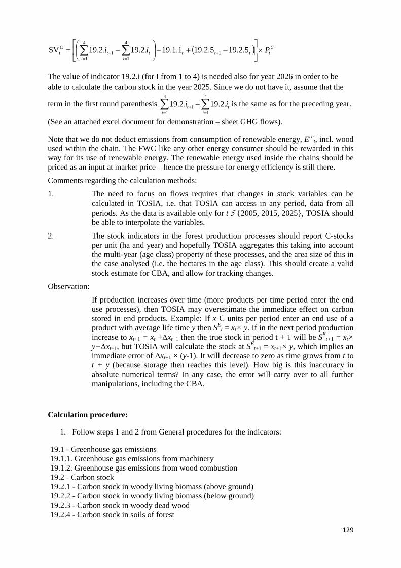
129
( ) Ctttt
it
it Pii ×
−+−
−= +
==+ ∑∑ 5.2.195.2.191.1.19.2.19.2.19SV 1
4
1
4
11
Ct
The value of indicator 19.2.i (for I from 1 to 4) is needed also for year 2026 in order to be able to calculate the carbon stock in the year 2025. Since we do not have it, assume that the
term in the first round parenthesis ∑∑==
+ −4
1
4
11 .2.19.2.19
it
it ii is the same as for the preceding year.
(See an attached excel document for demonstration – sheet GHG flows).
Note that we do not deduct emissions from consumption of renewable energy, Eret, incl. wood
used within the chain. The FWC like any other energy consumer should be rewarded in this way for its use of renewable energy. The renewable energy used inside the chains should be priced as an input at market price – hence the pressure for energy efficiency is still there.
Comments regarding the calculation methods:
1. The need to focus on flows requires that changes in stock variables can be calculated in TOSIA, i.e. that TOSIA can access in any period, data from all periods. As the data is available only for t 5 {2005, 2015, 2025}, TOSIA should be able to interpolate the variables.
2. The stock indicators in the forest production processes should report C-stocks per unit (ha and year) and hopefully TOSIA aggregates this taking into account the multi-year (age class) property of these processes, and the area size of this in the case analysed (i.e. the hectares in the age class). This should create a valid stock estimate for CBA, and allow for tracking changes.
Observation:
If production increases over time (more products per time period enter the end use processes), then TOSIA may overestimate the immediate effect on carbon stored in end products. Example: If x C units per period enter an end use of a product with average life time y then SE
t = xt× y. If in the next period production increase to xt+1 = xt +Δxt+1 then the true stock in period t + 1 will be SE
t+1 = xt× y+Δxt+1, but TOSIA will calculate the stock at SE
t+1 = xt+1× y, which implies an immediate error of Δxt+1 × (y-1). It will decrease to zero as time grows from t to t + y (because storage then reaches this level). How big is this inaccuracy in absolute numerical terms? In any case, the error will carry over to all further manipulations, including the CBA.
Calculation procedure:
1. Follow steps 1 and 2 from General procedures for the indicators:
19.1 - Greenhouse gas emissions 19.1.1. Greenhouse gas emissions from machinery 19.1.2. Greenhouse gas emissions from wood combustion 19.2 - Carbon stock 19.2.1 - Carbon stock in woody living biomass (above ground) 19.2.2 - Carbon stock in woody living biomass (below ground) 19.2.3 - Carbon stock in woody dead wood 19.2.4 - Carbon stock in soils of forest

130
2. Calculate 19.2.5 internally
3. Use formula ( ) Ctttt
it
it Pii ×
−+−
−= +
==+ ∑∑ 5.2.195.2.191.1.19.2.19.2.19SV 1
4
1
4
11
Ct
4. Follow steps 3, 5 and 6 from the General procedures (NOT step 4, as the shadow price of carbon is assumed to change NOT according to GDP/cap growth, but according to the table with €/kg of CO2 values).