monetary policy spillover to small open economies: is the
TRANSCRIPT
www.cnb.cz
Working Paper Series ——— 6/2021
Monetary Policy Spillover to Small Open Economies: Is the Transmission Different
under Low Interest Rates? Jin Cao, Valeriya Dinger, Tomás Gómez, Zuzana Gric,
Martin Hodula, Alejandro Jara, Ragnar Juelsrud, Karolis Liaudinskas, Simona Malovaná, Yaz Terajima
Cze
ch N
atio
nal B
ank
——
— W
orki
ng P
aper
Ser
ies
——
— 6
/202
1

The Working Paper Series of the Czech National Bank (CNB) is intended to disseminate the results of the CNB’s research projects as well as the other research activities of both the staff of the CNB and collaborating outside contributors, including invited speakers. The Series aims to present original research contributions relevant to central banks. It is refereed internationally. The referee process is managed by the CNB Economic Research Division. The working papers are circulated to stimulate discussion. The views expressed are those of the authors and do not necessarily reflect the official views of the CNB. Distributed by the Czech National Bank, available at www.cnb.cz Reviewed by: José-Luis Peydró (Imperial College London, ICREA-UPF-CREI-BarcelonaGSE,
CEPR)
Issued by: © Czech National Bank, November 2021
Monetary Policy Spillover to Small Open Economies: Is the TransmissionDifferent under Low Interest Rates?
Jin Cao, Valeriya Dinger, Tomás Gómez, Zuzana Gric, Martin Hodula, Alejandro Jara, RagnarJuelsrud, Karolis Liaudinskas, Simona Malovaná, and Yaz Terajima ∗
Abstract
We explore the impact of low and negative monetary policy rates in core world economies onbank lending in four small open economies – Canada, Chile, the Czech Republic and Norway –using confidential bank-level data. Our results show that the impact on lending in these small openeconomies depends on the interest rate level in the core. When interest rates are high, monetarypolicy cuts in core economies can reduce credit supply in small open economies. In contrast, wheninterest rates in core economies are low, further expansionary monetary policy increases lendingin small open economies, consistent with an international bank lending channel. These resultshave important policy implications, suggesting that central banks in small open economies shouldwatch for the impact of potential regime switches in core economies’ monetary policy when ratesshift to and from the very low end of the distribution.
Abstrakt
Zkoumáme dopad nízkých a záporných menovepolitických sazeb ve velkých svetovýchekonomikách na bankovní úvery ve ctyrech malých otevrených ekonomikách – Kanade, Chile,Ceské republice a Norsku – pomocí duverných dat na úrovni bank. Naše výsledky ukazují, žedopad na úverování v techto malých otevrených ekonomikách závisí na úrovni úrokových sazebv klícových ekonomikách. Když jsou úrokové sazby vysoké, uvolnení menové politiky vklícových ekonomikách muže snížit nabídku úveru v malých otevrených ekonomikách. Naprotitomu, když jsou úrokové sazby v klícových ekonomikách nízké, další expanzivní menovápolitika zvyšuje úverování v malých otevrených ekonomikách, což je v souladu s kanálemmezinárodního bankovního úverování. Tyto výsledky mají duležité politické dusledky.Naznacují, že centrální banky v malých otevrených ekonomikách by mely sledovat dopadpotenciálních zmen režimu v menové politice klícových svetových ekonomik, predevším potékdyž sazby klesají k velmi nízkým úrovním nebo z nich stoupají.
JEL Codes: E43, E52, E58, F34, F42, G21, G28.Keywords: Cross-border monetary policy spillover, international bank lending channel,
low and negative interest rate environment (LNIRE), portfolio channel.∗ Jin Cao, Norges Bank, [email protected] Dinger, University of Osnabrück and Leeds University Business School, [email protected]ás Gómez, Banco Central de Chile, [email protected] Gric, Czech National Bank and Masaryk University in Brno, [email protected] Hodula, Czech National Bank and Prague University of Economics and Business (Department of MonetaryTheory and Policy), [email protected] Jara, Banco Central de Chile, [email protected] Juelsrud, Norges Bank, [email protected] Liaudinskas, Norges Bank, [email protected] Malovaná, Czech National Bank and Prague University of Economics and Business (Department ofMonetary Theory and Policy), [email protected] Terajima, Bank of Canada, [email protected] authors thank José-Luis Peydró as well as participants of International Banking Research Network (IBRN)meetings and internal seminars of our institutions for their very valuable comments. This Working Paper shouldnot be reported as representing the views of Bank of Canada, Banco Central de Chile, Czech National Bank, orNorges Bank. The views expressed are those of the authors.

2Jin Cao, Valeriya Dinger, Tomás Gómez, Zuzana Gric, Martin Hodula, Alejandro Jara, RagnarJuelsrud, Karolis Liaudinskas, Simona Malovaná, and Yaz Terajima
1. Introduction
Since the Global Financial Crisis (GFC) of 2007–2009, policy rates in core world economies haveremained low relative to historical levels for a prolonged period of time. An extensive body ofliterature has focused mostly on the impact of this environment on domestic outcomes such asmonetary policy pass-through, bank profits, risk-taking, and credit allocation (Altavilla et al.,2021; Basten and Mariathasan, 2018; Bittner et al., 2020; Bottero et al., 2019; Brunnermeier andKoby, 2018; Eggertsson et al., 2019). However, considerably less attention has been given to thecross-border spillovers of such a policy, which is of particular relevance since monetary policyspillovers from the core economies can substantially limit the effectiveness of domestic monetarypolicy in small open economies (SOEs. See, for example, Cao and Dinger (2021)). In theory,expansionary monetary policy in a core economy has an ambiguous effect on the lending of banks– not only multinational banks, but also domestic banks – in an SOE.1 On the one hand, theinternational bank lending channel suggests that monetary expansion in the core makes moneymarket funding there cheaper, inducing banks in SOEs to increase their funding from the core andlend more in SOEs (Kashyap and Stein, 2000; Cetorelli and Goldberg, 2012). In contrast, theportfolio channel argues that lowering interest rates in the core improves borrowers’creditworthiness, inducing banks to shift credit supply away from SOEs (Adrian et al., 2014; Hillset al., 2019). Such ambiguous effects of cross-border monetary policy spillover are furthercomplicated by the current historically low interest rates in the core countries: Although the recentliterature shows that a low and negative interest rate environment (LNIRE) can distort monetarypolicy pass-through and bank lending within the core economies, there is almost no evidence onwhether cross-border monetary policy spillovers are modified by LNIRE in the core.
In this paper, we attempt to fill in this gap and investigate the role of monetary policy spillovers fromcore world economies to lending in SOEs, with particular attention to the degree of spillovers at lowor negative interest rates. We trace the impact of monetary policy shocks in three core economies –the US, euro area (EA), and UK – on lending in four SOEs – Canada, Chile, the Czech Republic, andNorway (CCCN hereafter). In the case of Norway, we also account for spillovers from Sweden, asthe same Scandinavian banks have a presence in both the Swedish and Norwegian banking sectors.We use proprietary data on bank lending in these four SOEs for the period 2002–2019. Employingsuch a long time horizon enables us to trace the monetary policy spillovers in times of substantialvariations in core economies’ interest rates and contrast low-interest-rate periods with periods ofhigher interest rates.2 Our main contribution to the existing literature is to examine how LNIRE inthe core shapes monetary policy spillovers to SOEs.
The availability of confidential bank-level data in the four economies gives us an opportunity toabstract from bilateral confounding effects while we can still explore a sample of sufficientlysimilar countries. The countries in our sample are all small, financially open economies, with asubstantial presence of global banks, and operate an inflation-targeting monetary policy regimewith flexible exchange rates (Table 1)3. Moreover, CCCN are all bank-oriented economies. InCanada and Norway, banks hold total assets of more than 100% of GDP; in Chile and the CzechRepublic, the size of the banking sector is smaller but still high compared to emerging economieson average. Also, bank credit is the main source of financing to the non-financial private sector inall four economies. CCCN’s banking sectors are highly concentrated, particularly in Canada and
1 We discuss this in more detail in Section 3.2 During our sample period, core countries’ monetary policy rates range from zero or negative to more than 5% –just before the GFC.3 The Czech Republic generally operates a managed floating exchange rate regime; however, during 2013–2017the CNB employed a temporary asymmetric exchange rate commitment against EUR.

Monetary Policy Spillover to Small Open Economies: Is the Transmission Different under LowInterest Rates? 3
Chile, where the 5-bank asset concentration is above 90% and 75%, respectively. Furthermore,banks’ cross-border exposure in terms of assets and liabilities is relatively high in all CCCNcountries, and accounts for 18% and 20% on average of total bank assets and liabilities,respectively. Also, the average share of foreign currency-denominated loans is 13% of totallending (excluding Canada), and 20% in the Czech Republic. These characteristics might beinformative about the role that foreign monetary policies play in shaping domestic lending inCCCN. On top of that, banking sectors in all four countries share important features exposing themto international shocks, including changes in foreign monetary policy rates. Although the fourcountries vary greatly in size – Canada, Chile, the Czech Republic, and Norway represent 1.4%,0.3%, 0.3%, and 0.5% respectively of global GDP at purchasing power parity rates as at 2019 –they are all small enough that the monetary policy of the core countries can be consideredexogenous to developments in the CCCN’s domestic sectors. Owing to their role as commodityexporters, the monetary policy of Canada, Chile and Norway is less synchronized with the globalbusiness cycles, implying that domestic policy rates can differ relative to the core economies.Emerging market status for Chile and the Czech Republic also contributes to differences in policyrates relative to the core.
Table 1: All Countries Share Similar Characteristics
Canada Chile CzechRepublic
Norway
Credit to non-financial sector from all sectors to GDPa 305% 188% 120% 284%Credit to non-financial sector from banks to GDPa 112% 88% 51% 80%5-bank asset concentrationb 92% 77% 66% 64%Share of foreign-owned banks in total assetsb 2% 44% 86% 29%Share of cross-border liabilities in total assetsb 9% 12% 24% 35%Share of cross-border assets in total assetsb 35% 6% 10% 21%Share of loans to private sector in foreign currencyb 0%d 11% 20% 8%Year of inflation-targeting adoption 1991 1999 1998 2001Currency regime Freely
floatingManagedfloating
Managedfloating
Freelyfloating
Capital mobility “Open” “Gate”c “Open” “Open”
Note: a As of 2019, according to the BIS total credit statistics database. b As of 2019Q4, according to internal informationfrom each central bank. c “Gate” means that a moderate share of types of cross-border financial transactions are subject tosignificant capital controls (see Fernández et al., 2016). d Since we define domestic loans in Canada as the loans given inCanadian dollars, the share of loans in foreign currency by default is zero.
We start the empirical analysis with a common framework across countries, allowing lending in allsample countries to be contingent on spillovers from all core countries. We first look at the impactof changes in short-term interest rates in core countries. We define a core policy rate as “low” if itis in the 1st quartile of its distribution; otherwise, we define it as “high”. As a part of this exercise,we also investigate the role of long-term interest rates. In particular, we explore whether changesin the yield curve matter for monetary policy spillovers conditional on the short-term policy rate.Next, we explore whether the effect on lending is driven by multinational banks, which may employtheir internal capital markets to channel funds across borders. In a more general sense, assumingthat frictions in the interbank market are not too pronounced, this channeling of funds can alsobe intermediated through the interbank market. In this case, we will observe spillover effects inthe lending dynamics of multinational and a wider population of banks. Last but not least, we digdeeper into exploring whether the lending response to changes in the core policy rate is uniformacross all lending categories, or whether it is driven by specific types of lending. We therefore look
4Jin Cao, Valeriya Dinger, Tomás Gómez, Zuzana Gric, Martin Hodula, Alejandro Jara, RagnarJuelsrud, Karolis Liaudinskas, Simona Malovaná, and Yaz Terajima
at the dynamics of different loan categories in response to changes in the core policy rate. Finally,we subject our results to a battery of robustness checks.
By employing a common empirical framework across countries, we reach four main conclusions.First, we find evidence of a portfolio channel effect when the core interest rate is high. Specifically,a decrease in a core interest rate when the interest rate is high leads to a decrease in lending inCCCN. In contrast, when the core policy rate is low, we find evidence of an international banklending channel at least in two of the four countries, Canada and Norway. A decrease in the corepolicy rate increases bank lending in SOEs during the period of low policy rates. These resultsare robust to different measures of monetary policy changes (such as variations in money marketrates or shock measures such as shocks recovered from an SVAR or the residuals from estimating aTaylor Rule), alternative estimation approaches, and a wide range of controls.
Second, both the portfolio and international bank lending channel remain at play even if weconsider long-term interest rates, proxied by changes in the yield curve. These channels areprominent especially in the Czech Republic and Norway. The results for Canada and Chile alsosupport the existence of both channels as they yield quantitatively and qualitatively similar results(the same size and direction of the effect). Not surprisingly, these results are less precise (notstatistically significant at the 5% level), given the relatively lower number of observations for thetwo latter countries.
Third, we show that multinational banks’ lending exhibits stronger spillover effects in Norway,while the opposite is true for Chile and the Czech Republic. The result for Norway provides somesupport for the existence of an internal capital market used by multinational banks to channel fundsacross borders in response to changes in the core policy rate. However, the mixed evidence mightalso be generated by the fact that well-functioning interbank markets are a fairly good substitutefor internal capital markets in terms of shifting liquidity. Moreover, while the majority of banks inChile and the Czech Republic are foreign-owned, both domestic and foreign banks face the sameregulation, limiting the use of the internal capital market.
Fourth, we show that, in all countries except the Czech Republic, the international bank lendingchannel at low rates operates primarily through mortgage lending and consumer loans. Similarresults are found for Chile and Norway when it comes to riskier corporate loans. The latter isconsistent with increased risk-taking associated with the international bank lending channel (Moraiset al., 2019).
Our paper fits into two strands of the literature. The first strand of studies focuses on the bankdimension of the cross-border transmission of monetary policy, in particular, on the transmissionof the core world economies’ monetary policy to other countries through banks’ exposure ininternational money and capital markets. For instance, Morais et al. (2019) identify how monetarypolicy in the core economies influences corporate lending in Mexico. They find that a foreignpolicy rate shock affects the supply of credit to Mexican firms mainly via their respective foreignbanks in Mexico. In contrast, investigating the transmission of global financial cycles to domesticcredit market conditions in Turkey, di Giovanni et al. (2021) find that an easing in global financialconditions is transmitted mostly by domestic banks that are more exposed to international capitalmarkets. Tracking components of banks’ balance sheets, Cao and Dinger (2021) document howforeign monetary policy, jointly with global risk factors, affects international banks’ domesticlending by changing their funding conditions, and how such an effect propagates through thedomestic money market where non-international banks borrow from international banks.

Monetary Policy Spillover to Small Open Economies: Is the Transmission Different under LowInterest Rates? 5
Furthermore, Bush et al. (2021) emphasize that international monetary policy spillovers todomestic lending can also be affected by the domestic macro-prudential policy stance.
The second strand of related literature explores the impact of a negative interest rate on bank lending.However, existing studies focus mainly on domestic transmission, especially on how bank lendingis affected by policy rate pass-through, i.e., how deposit rates and loan rates react to a low monetarypolicy rate. For instance, Bittner et al. (2020) find that a negative interest rate is less expansionaryin the core economy because the policy rate pass-through to deposit rates is more impaired; such animpaired bank lending channel under impaired monetary policy pass-through is also documented inEggertsson et al. (2019) for the case of Sweden. Bottero et al. (2019) and Basten and Mariathasan(2018) find that the bank lending channel is less impaired when banks are able to pass on the negativeinterest rate to depositors by increasing fees; similarly, Altavilla et al. (2021) find that sound banksare able to pass on negative interest rates to corporate depositors, and this incentivizes corporateborrowers to reduce cash holdings and increase investments, which strengthens the real effects ofmonetary expansion under negative interest rates.
Our main contribution to the existing literature is to investigate whether the level of the core’spolicy rate influences how core economies’ monetary policy spills over to small open economies.We document two novel findings. First, we show that the dominating channel of internationalmonetary policy spillovers varies with the level of the core’s policy rates. Specifically, we findevidence that the international bank lending channel is primarily active when the core’s policy ratesare at their historically low or negative levels. The portfolio channel appears to dominate wheninterest rates in the core are high. Using granular bank-level data from four SOEs spanning overalmost two decades including both periods under LNIRE and periods under higher interest rates,our results can therefore reconcile the seemingly contradictory results of existing studies that findevidence on either the international bank lending channel (for example, Morais et al. (2019)) or theportfolio channel (for example, Hills et al. (2019)), based on relatively shorter sample periods. Ourresults illustrate an international search-for-yield channel that is consistent with – but also adds aninternational angle to – the domestic search-for-yield literature on banking, such as Jiménez et al.(2014). Second, focusing on the period of LNIRE, we specifically show that low and negative policyrates in the core increase bank lending in SOEs.
The rest of the paper is organized as follows. In Section 2, we describe the main features andsources of data that are deployed in this paper. In Section 3, we present our conceptual frameworkand our main hypotheses for further tests. In Section 4, we investigate the spillover of monetarypolicy from the core to SOEs; in Section 5, we show how our results are robust to a wide variety ofmeasurements of monetary policy shocks in the core, as well as different specifications of regressionequations. Section 6 concludes.
2. Data and Measurements
In this section, we describe the main sources and features of our data. We combine severalquarterly datasets for the period of 2002–2019 for Canada, Chile, the Czech Republic and Norway.Bank-level balance sheet items come from the Office of the Superintendent of FinancialInstitutions (OSFI) for Canada, the former Superintendence of Banks and Financial Institutions(Superintendencia de Bancos e Instituciones Financieras, SBIF) of Chile4, the Czech NationalBank (CNB) for the Czech Republic, and Official Financial Reports by Banks and Financial4 On 1 June 2019, the SBIF was integrated into the Financial Market Commission (Comisison para el MercadoFinanciero or CMF, in Spanish).

6Jin Cao, Valeriya Dinger, Tomás Gómez, Zuzana Gric, Martin Hodula, Alejandro Jara, RagnarJuelsrud, Karolis Liaudinskas, Simona Malovaná, and Yaz Terajima
Undertakings (Offentlig Regnskapsrapportering fra Banker og Finansieringsforetak, ORBOF) forNorway.
In Canada, the OSFI supervises federally chartered commercial banks, trust and loan companies,and foreign bank branches. The sample of Canadian banks employed in the analysis consists ofnine banks, including the six largest banks, two smaller domestic banks and one foreignsubsidiary.5 Foreign branches are excluded from the sample as they are not subject to Canadiancapital regulations.
Chilean banks are heterogeneous across several dimensions, including size, business model, fundingstructure, and ownership origin, with 40% foreign-owned banks and one state-owned bank thataccounts for 10% of total assets. The sample included in this study focuses on internationally activebanks relevant to domestic markets, i.e. big and medium-sized banks as classified by Jara and Oda(2015).6 By the end of 2019, this group of banks totaled ten institutions, six domestically-owned,and four foreign-bank subsidiaries, and accounted for more than 95% of total banking sector assets.
In the Czech Republic, the CNB supervises domestic banks and subsidiaries and, to a limited extent,also branches of foreign banks. As of 2019Q4, the Czech banking sector consists of twenty-fourdomestic banks and subsidiaries, with the five largest accounting for nearly 70% of all assets in thebanking sector. Regarding the business model, the majority of banks provide funding to the privatenon-financial sector, with some focused solely on mortgage lending; in particular, the sample ofbanks employed in the analysis includes five building societies and two mortgage banks.
The Norwegian banking sector has a relatively high number of banks. As at 2019Q4, there are 99savings banks and 36 commercial banks in Norway; among the commercial banks, twelve areforeign-owned banks, including six subsidiaries and six branches. Commercial banks are limitedliability companies. Foreign commercial banks are either subsidiaries or branches of mostlySwedish and Danish banks. Savings banks (“sparebank”) were originally established byNorwegian municipalities as independent entities without external owners, taking deposits andproviding credit to local households and regional businesses. Nowadays the difference betweensavings banks and commercial banks is relatively small. For instance, savings banks andcommercial banks compete in the same credit markets.7
Table 2 summarizes the main set of variables used in our empirical analysis described in thefollowing section. As for left-hand side variables, we consider banks’ credit growth rates to theprivate sector, as well as credit to different sectors (mortgages, consumer, and corporate loans).Also, we include a traditional set of banks’ controls (deposits, capital adequacy, liquidity, and
5 For Canadian data, domestic lending is defined by loans in Canadian dollars. In addition,there was a large changein the reporting of federally regulated banks’ balance sheets in 2011Q4 due to the application of the InternationalFinancial Reporting Standards in Canada. We apply a dummy variable to control for its impact.6 In terms of the Jara and Oda (2015) bank taxonomy, retail banks are not internationally active, while tesoreriabanks do not participate in domestic credit markets.7 In our database some banks appear and/or disappear throughout the sample period, resulting in an unbalancedpanel. To account for entry and exit, we adopt different strategies depending on the scenario. In Chile, we accountfor mergers using a binary variable equal to one at the quarter of merger. The biggest mergers and acquisitionsoccurred in the 1990s and early 2000s (Ahumada et al. (2001)). In the Czech Republic, we do not record any majormerger or acquisition during the time span, while in Norway minor ones remain untreated. In Canada, the sampleof banks are selected to represent the balanced panel data and, while there are mergers and acquisitions by largeCanadian banks during the data, none of them are sizable.

Monetary Policy Spillover to Small Open Economies: Is the Transmission Different under LowInterest Rates? 7
financial security to total asset ratios), as well as macro-financial control variables (GDP growth,inflation, domestic interest rates, and time dummies).8
Table 2: Summary Statistics
Canada (9 banks) Chile (15 banks)Obs Min p25 p50 Mean p75 Max Obs Min p25 p50 Mean p75 Max
LHS: QoQ credit growth (%)Total 639 n.a. n.a. n.a. 6.5 n.a. n.a. 885 -8.7 0.3 1.9 2.5 3.9 83.6Mortgages 639 n.a. n.a. n.a. 6.1 n.a. n.a. 828 -14.8 1.2 2.5 3.1 4.3 74.6Consumer 639 n.a. n.a. n.a. 6.1 n.a. n.a. 828 -16.3 0.2 2.0 3.1 4.1 84.2Corporate 639 n.a. n.a. n.a. 5.2 n.a. n.a. 885 -8.8 -0.2 1.8 2.5 4.1 114.0Bank control variables (ratios in %)a
Deposits to liabilities 639 n.a. n.a. n.a. 53.8 n.a. n.a. 885 0.0 65.0 71.0 69.0 76.0 96.0Capital to assets 639 n.a. n.a. n.a. 5.6 n.a. n.a. 885 0.0 6.0 7.0 8.0 9.0 27.0Liquid assets 639 n.a. n.a. n.a. 11.6 n.a. n.a. 885 2.0 11.0 15.0 16.0 20.0 49.0Securities assets 639 n.a. n.a. n.a. 21.5 n.a. n.a. n.a. n.a. n.a. n.a. n.a. n.a. n.a.Macro-financial control variables (%)GDP growth 72 -9.1 1.0 2.3 2.0 3.5 5.9 72 -4.2 0.3 0.9 0.9 1.4 3.4Inflation rates 72 -3.9 1.1 1.7 1.9 2.9 5.3 72 -0.8 0.2 0.8 0.8 1.3 3.1Domestic interbank rate 72 0.4 1.2 1.5 2.0 2.8 4.9 72 0.4 2.7 3.4 3.7 5.0 8.2Domestic Spread 72 -0.3 0.8 1.1 1.4 2.1 3.4 62 -2.6 0.2 0.9 1.2 1.8 5.7Change in domestic rate 72 -1.5 0.0 0.0 0.0 0.1 0.5 72 -4.1 -0.2 0.0 -0.1 0.3 1.3Change in domestic Spread 72 -0.7 -0.2 -0.1 0.0 0.1 0.7 61 -2.3 -0.3 -0.1 -0.1 0.2 3.7Domestic Low IR period 72 0.0 0.0 0.0 0.3 0.5 1.0 72 0.0 0.0 0.0 0.3 1.0 1.0
Czech Republic (21 banks) Norway (226 banks)Obs Min p25 p50 Mean p75 Max Obs Min p25 p50 Mean p75 Max
LHS: QoQ credit growth (%)Total 1,353 -4.9 0.0 2.5 3.4 6.1 15.8 8,904 -35.3 0.4 2.1 3.1 3.9 88.9Mortgages 1,308 -9.2 0.2 3.0 4.3 7.1 22.8 8,134 -26.9 0.3 2.3 2.8 4.2 66.4Consumer 984 -27.0 -1.0 2.1 4.9 7.7 52.6 8,131 -100.0 -5.8 0.6 0.7 7.3 100.0Corporate 1,334 -12.8 -3.1 0.8 2.4 5.9 26.5 8,417 -57.2 -1.0 1.7 2.4 4.7 93.0Bank control variables (ratios in %)a
Deposits to liabilities 1378 0.0 60.8 77.7 73.3 96.9 100.0 8904 0.0 56.0 72.0 63.0 82.0 99.0Capital to assets 1378 1.4 5.9 7.9 10.4 11.1 99.6 8904 -16.0 7.0 9.0 10.0 12.0 100.0Liquid assets 1378 0.0 1.7 8.6 13.5 20.9 82.0 8904 0.0 3.0 5.0 8.0 8.0 100.0Securities assets 1295 0.0 5.8 16.5 20.9 32.4 76.8 8904 -7.0 6.0 9.0 10.0 13.0 85.0Macro-financial control variables (%)GDP growth 72 -3.4 0.4 0.7 0.7 1.2 2.7 72 -6.3 -3.2 -0.8 0.5 3.3 9.8Inflation rates 72 -0.8 0.1 0.4 0.5 0.7 3.9 72 -1.6 0.1 0.4 0.5 0.8 2.7Domestic interbank rate 72 0.3 0.5 1.7 1.7 2.4 4.3 72 0.8 1.5 2.1 2.7 3.1 7.2Domestic Spread 72 -0.8 0.7 1.3 1.3 2.0 3.4 72 -1.9 -0.1 0.5 0.5 1.2 2.8Change in domestic rate 71 -1.2 -0.2 0.0 0.0 0.1 0.6 71 -2.5 -0.1 0.0 -0.1 0.2 0.6Change in domestic Spread 71 -0.8 -0.4 0.0 0.0 0.2 2.1 71 -1.1 -0.3 -0.1 0.0 0.2 2.2Domestic Low IR period 72 0.0 0.0 0.0 0.3 1.0 1.0 72 0.0 0.0 0.0 0.3 0.5 1.0
Note: a In this table, we present bank control variables in percentages (ratios multiplied by 100) for more detail and bettercomparison between countries; in the actual regression, however, bank controls are included as simple ratios not multiplied by100. Remaining variables enter the regression in the same units as presented in this table.
8 For Canada, the summary statistics for banks exclude the numbers from the date of the accounting standardchange. In addition, some numbers are reported as “n.a.” for Canadian banks due to the privacy restrictionsassociated with the use of data from regulatory reports.

8Jin Cao, Valeriya Dinger, Tomás Gómez, Zuzana Gric, Martin Hodula, Alejandro Jara, RagnarJuelsrud, Karolis Liaudinskas, Simona Malovaná, and Yaz Terajima
Figure 1 displays the series of interest rates and monetary policy shocks, as well as the low-interestrate periods in the four core countries. We use the 3-month average interbank lending rate as ourstandard monetary policy measure (Christiano et al., 1999). However, we also show that our resultsare robust to alternative policy rate measures, such as shadow rates as defined by (Wu and Xia,2016, 2020), a residual from a Taylor Rule and monetary policy shocks from SVAR (Gertler andKaradi, 2015). We use the difference between the average 10-year government bond yield and theinterbank lending rate as our measure for the interest rate spreads. We define a period as a “lowinterest rate period” if the interbank rate of the core country is below its 1st quartile or negative.9
Figure 1: Interest Rates and Monetary Policy Shocks Employed in Our Analysis
-2
0
2
4
-1
0
1
2
2005 2010 2015 2020
USA
-5
0
5
-4
-2
0
2
2005 2010 2015 2020
Euro Area
-4
0
4
-2
0
2
2005 2010 2015 2020
UK
-2
0
2
4
-1
0
1
2
2005 2010 2015 2020
Sweden
3-month rate Spread Shadow rate TR residuals (rhs) MP shock (rhs)
Note: Shaded areas indicate low interest rate periods.
3. Conceptual Framework and Main Hypotheses
As a prerequisite, an understanding of the effect of core economies’ low (or even negative) interestrates on the dynamics of bank lending in SOEs requires an understanding of the general channelsof monetary policy spillovers. The literature so far has proposed two main channels working inopposite directions. First, the international bank lending channel (Bernanke, 1983, 1993; Kashyapand Stein, 2000; Cetorelli and Goldberg, 2012) presumes that following an expansionary monetary
9 Table A1 in the Appendix presents the main descriptive statistics of core countries’ interest rates, the quarter-on-quarter changes of interest rates, as included in our regression analysis below, and the low-interest rates periods.Notice that the interest rates thresholds that define low-interest rate periods in the case of the US, euro area, UK,and Sweden are 0.28, 0, 0.57, and 0, respectively.

Monetary Policy Spillover to Small Open Economies: Is the Transmission Different under LowInterest Rates? 9
policy shock in the core, internationally active banks may increase their lending in SOEs due totheir lower cost of funding. Morais et al. (2019) present empirical evidence for the effectiveness ofthis channel and also show that it is driven by search for yield in the sense that, when interest ratesin the core are low, banks borrow there and lend in high-yield destinations, i.e., the SOEs. The otherchannel, the portfolio channel, predicts the opposite effect: A tightening of core monetary policymay reduce the creditworthiness of core economies’ borrowers and reduce their collateral values,which may induce multinational banks to increase lending in SOEs (see Barbosa et al. (2018) andHills et al. (2019)). A loosening of core monetary policy can reverse these effects, thus reducinglending to SOEs. The contrasting predictions of these channels motivate us to empirically test thefollowing hypothesis:
H1: An expansionary monetary policy shock in the core leads to an expansion ofbank lending in the small open economies.
Finding support for this hypothesis will be consistent with the international bank lending channel,while rejecting it will deliver evidence for the portfolio channel.
Note that the effects described in the above two channels can be present even if the interest ratesin the core are not particularly low. Exploring the spillovers of low interest rates in particular,therefore, requires an examination of how these channels are reinforced or inhibited when monetarypolicy rates in the core are low or even negative. That is, for example, the international lendingchannel can be reinforced by particularly strong search-for-yield concerns at the very low end ofthe interest rate distribution. This effect can be accelerated even further if banks in core economiesperceive negative interest rates as a cost they can circumvent by cross-border portfolio rebalancing.On the other hand, the portfolio channel can be less effective when interest rates are generallylow, since the net worth of firms in the core is possibly less sensitive to a mild monetary policytightening in the lower range of the interest rate distribution. To examine how the importance ofthe above channels change in low and negative interest rate environments, we therefore test thefollowing hypothesis:
H2: An expansionary monetary policy shock in the core has stronger effects on banklending in the small open economies when core interest rates are low.
Next, we focus on documenting the channels behind these spillovers. We start by exploring therole of multinational banks. To this end, we lean on a recent literature which argues thatmultinational banks play a central role in cross-border spillover of monetary policy. As is shownby Bräuning and Ivashina (2020), multinational banks with affiliates in both core and SOEsallocate credit and raise funding on a “global” basis, taking into account spatial variation infunding costs and returns. Expansionary monetary policy in the core incentivizes these banks torebalance their global balance sheets, which may lead to changes in lending to the SOEs. Moraiset al. (2019) also identify multinational banks as the main drivers of core monetary policyspillovers to Mexico. These results are consistent with the existence of an internal capital market(Campbell et al., 2012) within multinational banks which could reinforce both the internationalbank lending and the portfolio channel. We explicitly test the conjectures about the role ofmultinational banks by formulating our third hypothesis:
H3: The spillover of monetary policy shocks in the core to the small open economiesis stronger for multinational banks that have operations in both the core and the smallopen economies.

10Jin Cao, Valeriya Dinger, Tomás Gómez, Zuzana Gric, Martin Hodula, Alejandro Jara,Ragnar Juelsrud, Karolis Liaudinskas, Simona Malovaná, and Yaz Terajima
Monetary policy also influences banks’ incentive to take risks (Jimenez et al., 2013), and this risk-taking channel also holds in the international context. For example, changes in funding conditionsdue to monetary policy spillovers can affect bank risk-taking in the SOEs. As a result of such a risk-taking channel, we would expect riskier bank lending categories to be more sensitive to monetarypolicy spillover from the core. This leads to our next hypothesis:
H4: The sensitivity of bank lending to the spillover of monetary policy shocks in thecore differs across loan categories.
Finally, we expect that the impact of a monetary expansion in a low interest rate environment alsodepends on banks’ expectations with regard to how long such an environment will persist. As isargued by Rajan (2006), when monetary policy rate remains “low for long”, the search-for-yieldincentive is stronger. We therefore expect the monetary policy spillovers in a low-rate environmentto also be influenced by banks’ expectations with regard to how long low or negative interest ratesin the core will last. This leads to our last hypothesis:
H5: When core policy rates are low, the effect of monetary policy spillover from thecore to the small open economies is stronger if banks expect monetary policy ratesin the core to stay low for a long period.
4. Monetary Policy Spillovers From the Core to Small Open Economies
We start by investigating the degree of monetary policy spillovers and whether these spilloverschange when the core policy rate is low. For this purpose, we estimate the following baselinemodel:
∆Yb,t =α0 +βc1 ∆rc
t +βc2 ∆Spreadc
t +βc3 Lowc
t +δc1 (∆rc
t ×Lowct )+
δc2 (∆Spreadc
t ×Lowct )+ γ1Xb,t−1 + γ2Zt−1 + fb + εb,t (1)
where ∆Yb,t is the quarter-on-quarter log-change in lending of bank b at time t in percentage points,∆rc
t is the quarter-on-quarter change (first difference) in interest rate in core country c, ∆Spreadct is
the quarter-on-quarter change (first difference) in the difference between the the 10-year governmentbond yield and 3-month interbank rate in core country c, Lowc
t is dummy equal to one for the periodwhen the interest rate in country c is low (i.e. below a 1st quartile value) or negative, fb are bankfixed effects. Zt represents the vector of macroeconomic controls (quarterly GDP growth, quarterlyCPI inflation) and Xb,t−1 the vector of lagging bank-level controls (deposits over liabilities, equityover assets, securities over assets, liquid assets over total assets).
In our empirical approach, we closely follow the model by Claessens et al. (2018), who regressbank’s net interest income (or ROA) on the 3-month market rate, the spread between the 3-monthand 10-year bond yields and a dummy variable for low interest rate periods, controlling for time-varying bank characteristics and macroeconomic controls, and including fixed effects. The proposedmethodology allows estimating the direct monetary policy spillovers from the core economies tolending in SOEs in the low and high interest rate environment, while controlling for other factors.By including SOEs’ GDP growth and CPI inflation (and later on also the core’s GDP growth andCPI inflation), we control for general economic conditions, acknowledging the difficulty to fullyaddress the endogeneity in monetary policy. Nevertheless, following one clear and well-establishedmodel specification allows for comparability across countries, which is one of the key benefits ofthis paper.

Monetary Policy Spillover to Small Open Economies: Is the Transmission Different under LowInterest Rates? 11
The model is constructed based on three main assumptions driving international monetary policyspillovers. First, global banks from the core economies may be incentivized to move funds abroadto seek higher return. Thus, they may increase credit supply to the receiving countries through theirinternal capital markets. Second, when the low interest rate environment in core economies squeezesglobal banks’ net interest margin at home, they may have the incentive to explore other sources ofprofit, which may incentivize their foreign subsidiaries to take higher risks. Third, low funding costsin core economies may encourage banks (both domestic- and foreign-owned) in SOEs to increasetheir funding from core economies, and hence affect bank lending within SOEs. All these argumentsare consistent with an international bank lending channel, while, as discussed in the introduction,portfolio channel arguments may work in the opposite direction.
Table 3 offers a cross-country comparison of the baseline model estimates. The model specificationin equation (1) is estimated for each core country separately. Hence, the table contains three columnsfor each country, exploring spillovers from the US, EA and UK, and an additional column forNorway that includes results focusing on Sweden as a core country. Estimates for a full list ofcontrol variables can be found in the Appendix.
When core policy rates are high, our results suggest that there are substantial spillovers (dependingon the countries, the transmission works either through short market rates or spreads), and thatexpansionary monetary policy in the core decreases lending in CCCN. This finding is consistentwith a portfolio channel, where lower core policy rates improve borrower quality and induce banksto reallocate credit away from the SOE and to the core. In economic terms, the estimated effects aresizeable. A 1 unit reduction in a core policy rate is associated with a 1.4–4.4 pp average decrease inquarter-on-quarter lending in the SOEs.
However, this relationship changes substantially when interest rates are low, as highlighted by thenegative coefficient on ∆rc ×Lowc. This suggests that lending in the SOEs reacts to changes in thecore interest rates significantly differently in the low interest rate period. When interest rates arelow, a decrease in the core policy rate is associated with faster growth in domestic bank lending,suggesting that the portfolio channel is outweighed by the international bank lending channel. Thiseffect is found significant in case of Canada, the Czech Republic and Norway. For the CzechRepublic, the relationship passes through changes in the spread of the EA rates, while for Canadaand Norway the effect transmits through US short market rates and those of the SE and UK,respectively.
To visualize our results, we calculate marginal effects at mean values of other covariates and plotthe adjusted effects for different values of interest rate and spread changes (see Figures B1–B3 inAppendix). The difference in effect between the two periods suggests that different transmissionchannels are at play. During the low interest rate period, marginal effects are mostly negative,as indicated by mostly downward sloping red lines. This suggests that larger positive (negative)changes in the core countries’ policy rates are associated with slower (faster) lending growth inSOEs, which serves as evidence supporting an international bank lending channel. In contrast,mostly upward sloping blue lines suggest the dominance of the portfolio channel when rates arehigh.
Based on our results, we are able to identify which core policy rates matter for the different countriesin our sample. In this respect, we find that changes to the market interest rates (as captured bychanges in the three-month inter-bank rates) in the euro area are associated with changes in lendingin all four countries. The UK rates matter for Chile, Norway and Canada (only when considering thechanges to the market rates, ∆rc
t ) and the US rates for Canada (only when considering the changes

12Jin Cao, Valeriya Dinger, Tomás Gómez, Zuzana Gric, Martin Hodula, Alejandro Jara,Ragnar Juelsrud, Karolis Liaudinskas, Simona Malovaná, and Yaz Terajima
to the market rates) and Norway. On top of that, we find that Norway is highly exposed to changesin the interest rates of its neighbor, Sweden.
Having investigated the general role of a low interest rate environment in international monetarypolicy spillovers, we next provide evidence on the transmission mechanisms, e.g. in terms of therole of international banks, variation across different types of lending and the duration of the lowinterest rate period.
Table 3: Baseline Results
Canada ChileUS EA UK US EA UK(1) (2) (3) (4) (5) (6)
∆rct 2.96** 3.71* 4.44** 0.47 2.18*** 1.36**
(1.46) (1.98) (1.95) (0.68) (0.56) (0.62)∆Spreadc
t 1.98 0.54 2.07 -0.16 0.54 -0.83***(1.33) (1.57) (1.57) (0.28) (0.44) (0.26)
Lowct 0.58 -1.15 -1.43* -0.57 -0.01 -0.30
(0.83) (1.02) (0.73) (0.68) (0.59) (0.77)∆rc
t ∗Lowct -38.69* -19.04 -10.10 -8.13 10.16 -1.67
(21.94) (14.38) (10.22) (8.60) (12.26) (2.97)∆Spreadc
t ∗Lowct -3.93 -2.71 -2.12 -0.51 -0.75 0.21
(2.42) (2.31) (2.50) (1.05) (0.91) (0.95)N 648 648 648 885 885 885No. of banks 9 9 9 15 15 15Adjusted R2 0.412 0.411 0.413 0.440 0.450 0.440
Czechia NorwayUS EA UK SE US EA UK(7) (8) (9) (10) (11) (12) (13)
∆rct 0.06 1.82*** 0.83 2.68*** 1.38*** 4.11*** 2.75***
(0.47) (0.59) (0.56) (0.38) (0.43) (0.50) (0.46)∆Spreadc
t 0.03 1.35*** 0.63 1.32*** 0.32 1.22*** 1.71***(0.45) (0.50) (0.57) (0.35) (0.30) (0.42) (0.40)
Lowct -1.70*** -1.45*** -1.93*** -2.90*** -0.54** -2.70*** -1.42***
(0.31) (0.38) (0.29) (0.30) (0.26) (0.32) (0.25)∆rc
t ∗Lowct -5.98 1.55 -3.83 -7.26*** -0.97 -7.63 -5.70**
(6.58) (7.50) (3.02) (2.27) (5.31) (6.88) (2.62)∆Spreadc
t ∗Lowct 0.13 -2.46** 0.08 -1.28 0.03 -0.28 -1.55**
(1.00) (1.11) (0.95) (0.92) (0.83) (0.94) (0.68)N 1,274 1,274 1,274 8,904 8,904 8,904 8,904No. of banks 21 21 21 226 226 226 226Adjusted R2 0.165 0.166 0.173 0.266 0.254 0.268 0.258
Note: The table presents the coefficient estimates of regression specification (1) whereby the dependent variable is a Q-o-Q growth (in %) in domestic lending (excl. interbank loans) by bank b in quarter t in a small open economy outlined ontop (Canada, Chile, the Czech Republic or Norway), and the dependent variables are (1) a quarterly change (first difference)in average 3-month interbank rate in a core country/currency c (US, EA, UK or SE) in quarter t, (2) a quarterly change (firstdifference) in the spread between the average 10-year government bond yield and the average 3-month interbank rate in currencyc in quarter t, (3) a dummy variable Low equal to 1 if the average 3-month interbank rate in currency c in quarter t was lower thanthe 25th percentile within years 2002-2019, and (4 and 5) interaction terms between dummy Low and the other two variables.The specification includes bank-fixed effects and time-varying bank and macro controls but for brevity they are not reported.Full tables can be found in appendix. Every column presents results for a different core country/currency c, and columns aregrouped by a small open economy. Note: ***, ** and * denote the 1%, 5% and 10% significance levels. Robust standard errorsin parentheses. Bank fixed effects and control variables included.

Monetary Policy Spillover to Small Open Economies: Is the Transmission Different under LowInterest Rates? 13
4.1 The Role of International Banks
We next test whether spillovers are bigger for multinational banks, in line with our third hypothesis.For this purpose, we define a dummy variable familyc
b capturing whether the bank b has a familymember (i.e. a branch, subsidiary or headquarter) belonging to the same banking group in a corecountry c. We form double and triple interaction terms to explore the differences.
The results of these estimations are presented in Table 4. During a low interest rate period, thefamilyc
b dummy plays a role especially in Norway. In particular, as indicated by the negative andstatistically significant coefficient on the triple interaction term between the short-term rate, dummy“Low” and dummy “Family”, the negative effect of the Swedish short-term rate on Norwegiandomestic bank lending when interest rates are low is much stronger for banks that have a familymember in Sweden. Similarly, the same effect of the UK short-term rate is stronger for banksthat have a family member in the UK. This lends support to the internal capital market channel,whereby banks with access to money markets or central bank liquidity in low interest rate countrieschannel that cheap liquidity to higher-yield countries. Potential limits to arbitrage, possibly causedby post 2008–2009 crisis regulations and evidenced by deviations in covered interest rate parity(CIP), might have contributed to making this possible.
The interpretation is less conclusive for the other countries, with effects often going in the oppositedirection. For example, the change in the core country’s spread during the low interest rate periodhas a positive significant effect on the domestic lending of Chilean banks with a family memberin the core but a negative effect on the domestic lending of Chilean banks without such a member.Similar effects can be observed for the Czech Republic.
Furthermore, when the core policy rate is high, the interaction terms with the familycb are mostly
not statistically significant, with the exception of Norway. Here we can see again a much strongerpositive reaction in the domestic lending of banks with a family member in the core country.
Nevertheless, the significant results for Norway and the lack of significance for other SOEs maybe explained by the fact that Norway has enough variation to test the triple interaction, as it has arelatively large group of banks. The lack of variation (low number of banks) in other countries canexplain why results are less precise. The mixed evidence might also be generated by the fact thatwell-functioning interbank markets are a fairly good substitute for internal capital markets in termsof shifting liquidity.

14Jin Cao, Valeriya Dinger, Tomás Gómez, Zuzana Gric, Martin Hodula, Alejandro Jara,Ragnar Juelsrud, Karolis Liaudinskas, Simona Malovaná, and Yaz Terajima
Table 4: The Role of International Banks
Canada ChileUS EA UK US EA UK(1) (2) (3) (4) (5) (6)
∆rct 2.96** 3.71* 8.72 0.08 2.95*** 1.62**
(1.46) (1.98) (6.55) (0.59) (0.76) (0.59)∆Spreadc
t 1.98 0.54 6.37 0.40 1.11** 0.07(1.33) (1.57) (9.23) (0.49) (0.47) (0.72)
∆rct ∗Lowc
t -38.69* -19.04 17.97 -13.29 15.39 -0.94(21.94) (14.38) (15.66) (16.52) (10.54) (3.64)
∆Spreadct ∗Lowc
t -3.93 -2.71 -8.17 -3.54*** -2.98*** -0.98(2.42) (2.31) (10.06) (0.74) (0.91) (1.00)
Lowct 0.58 -1.15 -1.44** -1.30** 0.51 -1.17***
(0.83) (1.02) (0.74) (0.52) (0.45) (0.32)Lowc
t ∗Familycb - - - - - -
∆rct ∗Familyc
b - - -4.83 0.76 -1.86 -0.80(7.22) (1.30) (1.23) (0.92)
∆Spreadct ∗Familyc
b - - -4.83 -1.71 -2.75*** -1.21(10.21) (1.05) (0.90) (1.12)
∆rct ∗Lowc
t ∗Familycb - - -31.63 9.64 -13.19 -1.91
(19.76) (17.40) (30.93) (4.97)∆Spreadc
t ∗Lowct ∗Familyc
b - - 6.79 5.26*** 5.46*** 3.57***(11.12) (1.56) (1.25) (1.15)
N 648 648 648 885 885 885No. of banks 9 9 9 15 15 15Adjusted R2 0.412 0.411 0.412 0.450 0.450 0.440
Czech Republic NorwayUS EA UK SE US EA UK(7) (8) (9) (10) (11) (12) (13)
∆rct 0.02 2.98 0.84 2.02*** 1.47*** 3.39*** 2.42***
(0.53) (1.88) (0.65) (0.34) (0.38) (0.40) (0.43)∆Spreadc
t 0.04 3.02* 0.68 0.96*** 0.45 1.28*** 1.57***(0.51) (1.63) (0.68) (0.31) (0.28) (0.33) (0.37)
∆rct ∗Lowc
t -4.54 -37.56* -3.43 -4.11** -2.72 -8.25* -1.40(7.43) (21.50) (3.61) (1.68) (3.83) (4.98) (1.87)
∆Spreadct ∗Lowc
t 0.41 -6.39** -1.02 -0.73 -0.36 -0.50 -1.74***(1.13) (3.20) (1.13) (0.71) (0.61) (0.69) (0.53)
Lowct -1.57*** 0.18 -2.10*** -2.39*** -0.75*** -2.40*** -1.19***
(0.35) (1.09) (0.35) (0.23) (0.21) (0.25) (0.20)Lowc
t ∗Familycb -0.63 -1.67 0.53 -4.59*** 2.44 -2.50 -2.61
(0.72) (1.09) (0.62) (1.60) (2.21) (1.82) (1.85)∆rc
t ∗Familycb 0.20 -1.24 -0.02 7.01*** -1.25 7.16** 3.76
(1.07) (1.94) (1.14) (2.27) (3.58) (3.01) (2.80)∆Spreadc
t ∗Familycb -0.03 -1.87 -0.15 3.65* -1.68 -0.74 1.65
(1.03) (1.71) (1.23) (2.19) (2.07) (2.86) (2.59)∆rc
t ∗Lowct ∗Familyc
b -6.76 44.72** -1.18 -26.72* 22.09 4.65 -49.70**(15.63) (22.62) (6.48) (14.25) (47.71) (44.48) (21.79)
∆Spreadct ∗Lowc
t ∗Familycb -1.31 4.49 3.50* -5.24 4.85 2.07 1.91
(2.39) (3.38) (2.03) (5.54) (7.19) (6.16) (5.56)N 1,274 1,274 1,274 8,904 8,904 8,904 8,904No. of banks 21 21 21 226 226 226 226Adjusted R2 0.162 0.174 0.174 0.271 0.254 0.272 0.262
Note: The table presents the coefficient estimates of a regression that is similar to specification (1) but includes a dummyvariable Family, which equals to 1 if bank b had a family member (a branch, a subsidiary or a headquarter) belonging tothe same banking group in both the small open economy outlined on top and the core country c. The dummy Family isinteracted with the dummy Low, the change in 3-month rate and the change in spread. The triple interactions test weather theresults revealed by interaction terms in the baseline regression are stronger/weaker for banks with family members in the corecountries. Note: ***, ** and * denote the 1%, 5% and 10% significance levels. Robust standard errors in parentheses. Bankfixed effects and control variables included.
Monetary Policy Spillover to Small Open Economies: Is the Transmission Different under LowInterest Rates? 15
4.2 Bank Lending Across Loan Categories
In Tables 5–7 we investigate whether the core monetary policy spillovers vary across loancategories. Our presumption is that the spillovers from core economies’ monetary policy mighthave a differential impact on different types of loans if risk varies across these loans. Wedifferentiate here between corporate, mortgage and consumer loans. Our results indicate that whencore policy rates are high, the transmission works to a varying degree through all loan categories,with corporate loans being affected in all countries by the rate of at least one core country. Inaddition, as the countries in our sample are small open economies, the export-import orientation offirms and the usage of foreign currency loans may play a role. For example, exporters use foreigncurrency loans as a natural hedge against exchange rate risk in the Czech Republic.10,11
The results with regard to the period of low interest rates indicate substantial differences acrosscountries and loan categories. More specifically, the negative effect of the core country’s interestrate changes seems to be passed on the SOEs mostly through mortgages and consumer loans wheninterest rates are low. For example, the interaction between the Lowc dummy and changes in corepolicy rates are significant and negative for Norway and Chile in the case of both mortgage andconsumer loans and Canada for mortgage loans, consistent with a search-for-yield channel in thelow interest rate environment. This channel appears strong with SE, UK and EA rates for Norway,and all three rates for Canada and Chile. The effect on corporate loans is significant and negative,however, only for Chile (US rate) and Norway (SE rate).
10 The share of foreign currency loans in banks’ total corporate loans grew from around 10% to 30% during theperiod analyzed in the Czech Republic. The share of the foreign currency loans of the 1,000 largest exporters washigher, accounting for more than half of banks’ loan portfolio as of 2018.11 For Chile, we also find differences depending on the currency in which the loan is denominated (not reported).

16Jin Cao, Valeriya Dinger, Tomás Gómez, Zuzana Gric, Martin Hodula, Alejandro Jara,Ragnar Juelsrud, Karolis Liaudinskas, Simona Malovaná, and Yaz Terajima
Table 5: Spillovers Across Loan Categories – Mortgage Lending
Canada ChileUS EA UK US EA UK(1) (2) (3) (4) (5) (6)
∆rct 4.59** 5.98*** 8.22*** -0.63 0.61 0.21
(1.83) (2.21) (2.16) (0.76) (0.76) (0.82)∆Spreadc
t 2.58 0.09 3.60* -0.49 0.52 0.01(1.67) (1.93) (2.11) (0.77) (0.76) (0.98)
Lowct 2.44*** -2.77* -0.99 -0.21 -0.41 -0.69**
(0.92) (1.48) (0.86) (0.36) (0.55) (0.30)∆rc
t ∗Lowct -60.37* -46.83*** -24.66* -25.44** 2.26 -2.00
(31.32) (16.81) (14.62) (11.14) (12.61) (2.59)∆Spreadc
t ∗Lowct -5.43** -0.72 -2.99 0.23 -1.49 0.65
(2.58) (2.54) (2.80) (1.68) (1.13) (1.15)N 648 648 648 828 828 828No. of banks 9 9 9 14 14 14Adjusted R2 0.464 0.462 0.466 0.390 0.390 0.390
Czech Republic NorwayUS EA UK SE US EA UK(7) (8) (9) (10) (11) (12) (13)
∆rct 0.29 1.69** 0.85 1.57*** -0.14 2.76*** 1.87***
(0.68) (0.86) (0.81) (0.39) (0.42) (0.43) (0.46)∆Spreadc
t -0.15 1.32* 0.63 0.44 -0.38 0.53 0.29(0.66) (0.73) (0.83) (0.31) (0.27) (0.34) (0.36)
Lowct -1.45*** -2.31*** -1.68*** -1.88*** -0.62*** -1.86*** -0.70***
(0.46) (0.55) (0.44) (0.23) (0.21) (0.25) (0.21)∆rc
t ∗Lowct -5.42 -2.55 -1.55 -4.87** 2.83 -6.94 -1.28
(9.59) (10.93) (4.44) (1.95) (3.96) (5.60) (1.98)∆Spreadc
t ∗Lowct 1.38 -1.72 0.05 -1.80** 0.85 -1.36* 0.75
(1.46) (1.61) (1.39) (0.81) (0.65) (0.79) (0.58)N 1,229 1,229 1,229 8,134 8,134 8,134 8,134No. of banks 21 21 21 226 226 226 226Adjusted R2 0.215 0.130 0.141 0.207 0.200 0.209 0.202
Note: The table presents the coefficient estimates of regression specification (1) that was used for the baseline results but herethe dependent variable includes only mortgage loans. Note: ***, ** and * denote the 1%, 5% and 10% significance levels.Robust standard errors in parentheses. Bank fixed effects and control variables included.

Monetary Policy Spillover to Small Open Economies: Is the Transmission Different under LowInterest Rates? 17
Table 6: Spillovers Across Loan Categories – Consumer Lending
Canada ChileUS EA UK US EA UK(1) (2) (3) (4) (5) (6)
∆rct -1.69 1.82 0.90 -0.19 4.19*** 2.43*
(1.81) (2.39) (2.18) (0.87) (1.20) (1.41)∆Spreadc
t 2.21 3.25 3.12 -0.82 2.00* 0.44(1.60) (1.99) (2.14) (0.97) (1.13) (1.49)
Lowct -3.09*** -5.10*** -5.40*** -0.68 -2.43*** -2.26***
(1.02) (1.15) (0.90) (0.53) (0.84) (0.49)∆rc
t ∗Lowct -16.06 14.72 -2.03 -4.11 -1.95 -5.11*
(22.84) (13.44) (12.52) (13.77) (12.30) (3.01)∆Spreadc
t ∗Lowct -2.35 -4.83* -3.18 1.85 -2.55* -1.08
(2.93) (2.81) (2.76) (2.58) (1.30) (1.53)N 648 648 648 828 828 828No. of banks 9 9 9 14 14 14Adjusted R2 0.209 0.222 0.223 0.220 0.240 0.230
Czech Republic NorwayUS EA UK SE US EA UK(7) (8) (9) (10) (11) (12) (13)
∆rct 4.08** 5.24** 3.12 0.06 9.35*** 2.13* 1.59
(2.03) (2.56) (2.44) (1.08) (1.45) (1.22) (1.19)∆Spreadc
t 0.75 1.53 1.86 0.41 0.97 0.55 2.34**(1.99) (2.17) (2.53) (0.93) (0.79) (1.00) (1.11)
Lowct -0.04 -4.33** 0.67 -2.59*** 0.46 -2.40*** -0.62
(1.50) (1.69) (1.34) (0.68) (0.58) (0.74) (0.58)∆rc
t ∗Lowct -30.71 -16.05 5.87 -11.31** -4.08 -23.36 -14.31***
(28.42) (32.30) (13.13) (5.38) (11.71) (16.58) (5.50)∆Spreadc
t ∗Lowct -0.48 -5.65 -0.78 0.41 2.37 6.67*** -1.10
(4.30) (4.76) (4.11) (2.35) (1.88) (2.30) (1.62)N 910 910 910 8,128 8,128 8,128 8,128No. of banks 18 18 18 226 226 226 226Adjusted R2 0.001 0.010 -0.004 0.028 0.034 0.029 0.028
Note: The table presents the coefficient estimates of regression specification (1) that was used for the baseline results but herethe dependent variable includes only consumer loans. Note: ***, ** and * denote the 1%, 5% and 10% significance levels.Robust standard errors in parentheses. Bank fixed effects and control variables included.

18Jin Cao, Valeriya Dinger, Tomás Gómez, Zuzana Gric, Martin Hodula, Alejandro Jara,Ragnar Juelsrud, Karolis Liaudinskas, Simona Malovaná, and Yaz Terajima
Table 7: Spillovers Across Loan Categories – Corporate Lending
Canada ChileUS EA UK US EA UK(1) (2) (3) (4) (5) (6)
∆rct 3.53 6.20** 1.67 0.42 1.53** 1.02
(2.45) (3.11) (2.95) (0.75) (0.63) (0.68)∆Spreadc
t 1.64 2.87 -3.16 -0.59 -0.57 -1.04(2.71) (2.73) (3.06) (0.72) (0.66) (0.84)
Lowct 0.57 4.51** 2.63 -0.18 0.60 -0.89***
(1.81) (2.17) (1.85) (0.41) (0.50) (0.31)∆rc
t ∗Lowct -19.24 3.05 19.53 -24.83* 7.24 -2.26
(38.13) (45.51) (20.18) (14.52) (13.29) (3.45)∆Spreadc
t ∗Lowct -0.60 -6.67 5.50 -1.14 0.37 2.08*
(5.41) (6.96) (5.90) (1.31) (1.13) (1.10)N 648 648 648 885 885 885No. of banks 9 9 9 15 15 15Adjusted R2 0.020 0.034 0.028 0.410 0.410 0.420
Czech Republic NorwayUS EA UK SE US EA UK(7) (8) (9) (10) (11) (12) (13)
∆rct 2.04** 2.95** 2.85** 2.28*** 0.05 3.46*** 1.80***
(0.94) (1.19) (1.12) (0.51) (0.60) (0.64) (0.64)∆Spreadc
t 0.82 2.06** 1.06 1.12** 0.16 1.61*** 1.08*(0.92) (1.00) (1.16) (0.48) 0.41 (0.53) (0.56)
Lowct -1.10* -3.17*** -2.05*** -2.38*** -1.02*** -2.41*** -1.72***
(0.63) (0.75) (0.59) (0.40) (0.33) (0.44) (0.33)∆rc
t ∗Lowct -8.48 -1.27 -7.40 -5.35* -1.20 -10.06 -0.64
(13.22) (14.97) (6.08) (2.94) (6.90) (8.38) (3.05)∆Spreadc
t ∗Lowct 1.28 -2.35 0.89 -1.14 0.16 -1.10 -0.79
(2.01) (2.21) (1.90) (1.25) (1.04) (1.19) (0.89)N 1,260 1,260 1,260 8,417 8,417 8,417 8,417No. of banks 21 21 21 226 226 226 226Adjusted R2 0.064 0.080 0.072 0.102 0.096 0.103 0.099
Note: The table presents the coefficient estimates of regression specification (1) that was used for the baseline results but herethe dependent variable includes only corporate loans. Note: ***, ** and * denote the 1%, 5% and 10% significance levels.Robust standard errors in parentheses. Bank fixed effects and control variables included.

Monetary Policy Spillover to Small Open Economies: Is the Transmission Different under LowInterest Rates? 19
5. Robustness Checks
In this section we explore the sensitivity of our main results to changing the definition of coreeconomy monetary policy shocks, the set of control variables as well as the estimation approach.
5.1 Alternative Monetary Policy Indicators
In the baseline regression, we use the 3-month average interbank lending rate as our standardmeasure for monetary policy in the core. However, this variable may capture not only monetarypolicy shocks but also a prolonged environment of low rates when small or little variation wasobserved while the impact was still evident. As Christiano et al. (1999) argue, there is still littleconsensus in the literature on the measurement of monetary policy shocks. Therefore, we examinewhether our baseline results are robust to using several alternative monetary policy indicators thatare typically used in the literature: (i) shadow rates; (ii) residuals from SVAR, (iii) residuals fromthe Taylor Rule and (iv) a proxy variable for a prolonged period of low rates.
5.1.1 Shadow RatesThe first alternative we explore is shadow rates, which especially during periods when the zerolower bound (ZLB) is binding might substantially deviate from reported monetary policy rates andinterbank rates. In countries where the ZLB is applicable, policy as well as interbank interest rateshave been stuck at the lower bound and no longer necessarily convey all relevant information aboutthe stance of monetary policy, as central banks have introduced several unconventional monetarypolicy tools. For example, the US, the UK, as well as the euro area have performed several roundsof quantitative easing. The shadow rate is a measure of the effective monetary stimulus when theseunconventional tools are also taken into account. To explore robustness with regard to shadow rates,we replace the 3-month market rate with shadow rates (see Figure 1) that we estimate following theapproach of Wu and Xia (2016, 2020).
The shadow rates are computed using information from longer-term interest rates to infer ahypothetical short-term interest rate in the absence of a ZLB. Empirically, the shadow rate isextracted from the term structure of interest rates, especially medium- and long-term interest rates.As shadow rates are estimated using the whole yield curve, they enter the model specificationalone, that is, without the yield curve spreads. In addition, we keep the definition of the lowinterest rate period as before for comparability of estimates (i.e. the period is the same as in thebaseline regression).
The full regression results are presented in Table C6 in the Appendix, demonstrating that our mainresults are robust to using shadow rates. The estimates on the coefficients of interest rates remainquantitatively and qualitatively very similar, even though their precision decreases in someinstances. In other words, an increase in the core’s shadow rate has a positive effect on lending inthe SOE when interest rates are high and a negative effect if they are low or negative.
The evidence for the international bank lending channel during the low interest rate period remainstatistically significant for the Czech Republic and Norway, while revealing some additionalchannels for Canada. Specifically, Canadian lending responds significantly to monetary policychanges in the euro area and UK. Our results with shadow rates also reveal an additional channelfrom euro area monetary policy to Norwegian domestic lending at low rates which is not present inour baseline specification, consistent with unconventional monetary policy in the euro area havinga significant impact on bank lending in Norway. The effect for Chile remains statistically not

20Jin Cao, Valeriya Dinger, Tomás Gómez, Zuzana Gric, Martin Hodula, Alejandro Jara,Ragnar Juelsrud, Karolis Liaudinskas, Simona Malovaná, and Yaz Terajima
significant while the sign of estimated coefficients points to the same direction as for the otherthree small open economies. The picture is very similar during the period of high interest rates,supporting our previous evidence for the portfolio channel.
Finding robust estimation results when using shadow rates instead of short-term interbank ratesemphasizes the importance of longer interest rates in the identified transmission channels. Asevident from our baseline results, both portfolio and international bank lending channels remain atplay if we consider a proxy for changes in the yield curve, calculated as a spread between long andshort rates. Not surprisingly then, the alternative specification with shadow rates providesconsistent results as they are estimated using the whole yield curve. Hence, we suspect that thetransmission is affected not only by monetary policy surprises (shocks) but also by expectationsabout the future path of monetary policy. Next, we focus on the two components, i.e. residualsfrom SVAR and residuals from the Taylor rule.
5.1.2 Residuals From SVAR and the Taylor RuleIn our next robustness exercise, we address the issue that bank lending in SOEs may be drivenby banks’ expectation about monetary policy in the core that in turn is likely to reflect global realeconomic dynamics. In this sense, both bank lending in SOEs and monetary policy in the coremay be driven by confounding expectations about global economic developments. To sharpen theidentification and focus on unexpected changes in monetary policy, we now adopt two alternativemeasures of monetary policy shocks from the core: (1) the residual of SVAR, based on Gertler andKaradi (2015)12, or (2) the residual from the Taylor Rule, such that monetary policy shocks areproxied by the Taylor-rule residuals obtained by regressing the core country’s 3-month interbankrate on GDP growth and inflation.13 Residuals above zero indicate monetary policy tightening,while residuals below zero proxy for monetary policy easing.
In Table C7 in the Appendix we present the results based on the residual of SVAR, and in TableC8 in the Appendix we present the results based on the residual of the Taylor rule. In the caseof the Taylor rule residual we find that the results are qualitatively comparable to those of ourbaseline model. With regard to the SVAR residual the results are also comparable but the statisticalsignificance of the estimates is lower.
5.1.3 Persistently Low Interest RatesBanks are unlikely to substantially change their behavior if the low level of core economies’ interestrates is only transitory. Next, we therefore investigate whether the monetary policy spillovers ina low rate environment depend on whether or not the interest rate is expected to stay low for along period of time. In the baseline model, we use the difference between the average 10-yeargovernment bond yields and the interbank lending rate, or, the interest rate spread, as a measureof the market’s expectation regarding the future monetary policy stance in the core. In this sectionwe explicitly focus on the role of the duration of the low interest rate period. For this purpose, weinclude a “low-for-long” variable, Low for longc , which is defined as the number of consecutivequarters in which the Lowc dummy is equal to one (i.e. the 3-month interest rate has been below itsfirst quartile).
12 The SVAR residuals are based on a VAR considering output, inflation and a variety of interest rates. The VARis identified using daily data and changes in fed funds futures occuring on FOMC days.13 The residuals are estimated using OLS regression.

Monetary Policy Spillover to Small Open Economies: Is the Transmission Different under LowInterest Rates? 21
Results of the estimation of equation (1) including the Low for longc variable are reported in TableC9 in the Appendix. Similarly to the previous exercises, we reach quantitatively and qualitativelysimilar estimates of the coefficients on interest rates which supports our main results. On top ofthat, we find a statistically significant role of the length of the period during which interest ratesremain low or negative. With each subsequent quarter of the core’s interest rates being below their1st quartile, the lending dynamics in SOEs is generally more subdued. The effect linked to theprolonged period of low rates more or less replaces the effect previously identified on the Lowc
dummy, suggesting that not only the level of rates matter but also the length of the period when theyare at low levels.
Not surprisingly, we find a stronger and statistically significant reaction of SOEs’ bank lendingto the core’s spreads in the specification with the Low for longc variable. By controlling for theeffect of each subsequent quarter of low rates, we reveal the impact of changing expectations aboutthe core’s monetary policy (captured by a rotating yield curve) on SOEs’ lending. Specifically, adecrease in the slope of the yield curve at low rates translates to higher lending dynamics in Canadaand Norway, expanding on our baseline results.
5.2 Alternative Sets of Control Variables
5.2.1 Including Domestic RatesIn the next step, we include domestic interest rates (3-month interbank rate and spread) in thesame structure as the foreign ones in order to control for domestic monetary conditions. TableC10 presents the results. During the low interest rate period, the negative significant effect of acore country’s interest rates on domestic bank lending is preserved for most countries, compared tobaseline specification. For some countries, the effect is stronger (Chile) while for others there is aswitch of the significance from one core country’s rates to another (Canada and the Czech Republic).For Norway, the results appear to be mostly robust. We presume that the different outcomes fromincluding domestic interest rates are driven by the varying correlation between domestic rates andthose in the respective core economy. Moreover, consistently with the existence of a domestic banklending channel, both domestic short-term rates and spread receive negative coefficients for mostcountries with the exception of Chile. During a period of high rates, the estimates remain fairlysimilar to the baseline specification.
5.2.2 Macroeconomic Controls for the CoreWe start by including the inflation rate and the GDP growth rate of core countries to account forpotential omitted variable bias and potential confounding effects related to the fact that banklending might be affected by expected global trends in real economic dynamics and real interestrates rather than by loan supply shifts. The results presented in Table C11 indicate that when ratesare high, including these additional controls does not qualitatively change the estimatedcoefficients. However, during low-interest rates periods, the results are robust to this newspecification for the Czech Republic and Norway, while the estimates become imprecise forCanada and Chile. This divergence across countries might be driven by a varying intensity of realeconomic links between the core and the SOEs. Following Section 5.1.3, we also include thelow-for-long dummy here to account for the quarter duration of these periods (Table C11). Formost cases, this dummy variable proves to be negative and statistically significant, absorbingpartially the effects previously attributed to interest rates. Further, we add currency pairs betweenthe core and CCCN and the foreign currency structure of bank funding in the CCCN.

22Jin Cao, Valeriya Dinger, Tomás Gómez, Zuzana Gric, Martin Hodula, Alejandro Jara,Ragnar Juelsrud, Karolis Liaudinskas, Simona Malovaná, and Yaz Terajima
5.2.3 Bank-level ControlsNext, we explore whether our results are robust to expanding the set of bank-level control variablesthat can pick loan supply effects not necessarily related to monetary policy shocks in coreeconomies. We expand the set of controls by including additional bank-level controls, such as banksize, non-performing loans to total loans ratio, and changes in the house price index. We do notinclude these controls in the main specification to retain a tractable number of parameters toestimate and assure cross-country comparability that we cannot guarantee in the most saturatedspecifications since not all additional controls are available for all countries. The results of thisrobustness exercise indicate that in general, adding more controls does not affect our mainestimates.
5.2.4 Alternative EstimationsLast but not least, we turn our attention to employing alternative estimation approaches. For thispurpose, in an unreported test, we first consider a dynamic model specification instead of a static oneto check for the potential missing variable issue. Reassuringly, estimates related to the coefficientsof interest remain quantitatively and qualitatively unchanged.
In unreported tests, we also estimate additional specifications, considering: (i) annual instead ofquarter-to-quarter changes of the dependent variable, (ii) different winsorization schemes, (iii)richer lag structure, (iv) contemporaneous macro controls instead of lagged ones, (v) excluding theinterest rate spread or using it in level. In all these cases, we observe little to no change in our mainestimates.
Finally, in unreported tests we use a dummy variable “easing” interacted with our variables ofinterest from the baseline specification in order to test if our main results are symmetric in the casesof monetary policy tightening and easing. Our estimates do not indicate any asymmetry.
6. Concluding Remarks
Exploring proprietary bank-level data for four countries – Canada, Chile, the Czech Republic, andNorway – we provide evidence on the monetary policy spillovers from core world economies tolending in the small open economies. The main take-away of our analysis is that low interest ratesin the core – the US, euro area and UK – reinforce the existence of an international bank lendingchannel. In other words, when interest rates in the core countries are low, further expansionarymonetary policy in these countries is associated with increased lending in small open economies. Incontrast, when interest rates are relatively high, a core economy’s monetary policy expansion canresult in shrinking lending volumes in SOEs. This suggests that the portfolio channel dominatesoutside the low interest rate period.
We subject our main analysis to a battery of robustness checks, which support our main results andfurther expand our understanding of transmission channels. First, long-term yields and expectationsabout the future path of the core’s monetary policy seems to play an important role in the identifiedtransmission. Specifically, lower long-term yields in the core during the low rate periods tend tocontribute to higher lending in the small open economies. Second, we find evidence of internalcapital markets fueling the transmission in Norway, as lending by multi-national banks exhibitsstronger spillover effects; however, the results for other countries show quite the opposite. Third, theinternational bank lending channel at low rates operates through different types of loans, reflectingthe specifics of each economy and risk-taking associated with this channel.

Monetary Policy Spillover to Small Open Economies: Is the Transmission Different under LowInterest Rates? 23
The presented results provide an improved understanding of the impact of monetary policy cross-border spillovers and help reconcile the existence of both a portfolio channel and an internationalbank channel. In terms of policy implications, they illustrate that central banks should watch forpotential regime switches in the impact of core monetary policy when rates shift to and from thevery low end of the distribution. That is, for example, while monetary policy expansions in thecore might initially tighten local credit supply in small open economies, the credit supply couldstart increasing once core economies’ rates drop to a sufficiently low level. The reverse is likely tohappen once the core starts tightening its monetary policy.

24Jin Cao, Valeriya Dinger, Tomás Gómez, Zuzana Gric, Martin Hodula, Alejandro Jara,Ragnar Juelsrud, Karolis Liaudinskas, Simona Malovaná, and Yaz Terajima
References
ADRIAN, T., E. ETULA, AND T. MUIR (2014): “Financial Intermediaries and the Cross-sectionof Asset Returns.” The Journal of Finance, 69(6):2557–2596.
AHUMADA, A., J. MARSHALL, ET AL. (2001): “The Banking Industry in Chile: Competition,Consolidation and Systemic Stability.” BIS Background Paper, 45.
ALTAVILLA, C., L. BURLON, M. GIANNETTI, AND S. HOLTON (2021): “Is There a Zero LowerBound? The Effects of Negative Policy Rates on Banks and Firms.” Journal of FinancialEconomics, forthcoming.
BARBOSA, L., D. BONFIM, S. COSTA, AND M. EVERETT (2018): “Cross-border Spilloversof Monetary Policy: What Changes During a Financial Crisis?” Journal of InternationalMoney and Finance, 89:154–174.
BASTEN, C. AND M. MARIATHASAN (2018): “How Banks Respond to Negative Interest Rates:Evidence from the Swiss Exemption Threshold.” CESifo Working Paper Series 6901,CESifo Group Munich.
BERNANKE, B. S. (1983): “Irreversibility, Uncertainty, and Cyclical Investment.” The QuarterlyJournal of Economics (MIT Press), 98(1):85–106.
BERNANKE, B. S. (1993): “Credit in the Macroeconomy.” Quarterly Review, Federal ReserveBank of New York.
BITTNER, C., D. BONFIM, F. HEIDER, F. SAIDI, G. SCHEPENS, AND C. SOARES (2020): “WhySo Negative? The Effect of Monetary Policy on Bank Credit Supply Across the Euro Area.”Mimeo, European Central Bank.
BOTTERO, M., C. MINOIU, J.-L. PEYDRÓ, A. POLO, A. F. PRESBITERO, AND E. SETTE (2019):“Negative Monetary Policy Rates and Portfolio Rebalancing: Evidence from Credit RegisterData.” Working Paper 19/44, International Monetary Fund.
BRÄUNING, F. AND V. IVASHINA (2020): “Monetary Policy and Global Banking.” Journal ofFinance, 75(6):3055–3095.
BRUNNERMEIER, M. K. AND Y. KOBY (2018): “The Reversal Interest Rate.” WorkingPaper 25406, National Bureau of Economic Research.
BUSH, G., T. GÓMEZ, A. JARA, D. MORENO, K. STYRIN, AND Y. USHAKOVA (2021):“Macroprudential Policy and the Inward Transmission of Monetary Policy: The Case ofChile, Mexico, and Russia.” Review of International Economics, 29(1):37–60.
CAMPBELL, J. R., C. L. EVANS, J. D. FISHER, AND A. JUSTINIANO (2012): “MacroeconomicEffects of Federal Reserve Forward Guidance.” Brookings Papers on EconomicActivity 43(1), The Brookings Institution.
CAO, J. AND V. DINGER (2021): “Financial Globalization and Bank Lending: The Limits ofDomestic Monetary Policy.” Journal of Financial and Quantitative Analysis, forthcoming.
CETORELLI, N. AND L. S. GOLDBERG (2012): “Banking Globalization and MonetaryTransmission.” Journal of Finance, 67(5):1811–1843.
CHRISTIANO, L. J., M. EICHENBAUM, AND C. L. EVANS (1999): Chapter 2: MonetaryPolicy Shocks: What Have We Learned and to What End?, volume 1 of Handbook ofMacroeconomics, pages 65–148. Elsevier.

Monetary Policy Spillover to Small Open Economies: Is the Transmission Different under LowInterest Rates? 25
CLAESSENS, S., N. COLEMAN, AND M. DONNELLY (2018): “Low-for-long Interest Rates andBanks’ Interest Margins and Profitability: Cross-country Evidence.” Journal of FinancialIntermediation, 35(A):1–16.
DI GIOVANNI, J., S. KALEMLI-ÖZCAN, M. F. ULU, AND Y. S. BASKAYA (2021): “InternationalSpillovers and Local Credit Cycles.” Review of Economic Studies, forthcoming.
EGGERTSSON, G. B., R. E. JUELSRUD, L. H. SUMMERS, AND E. G. WOLD (2019): “NegativeNominal Interest Rates and the Bank Lending Channel.” Working Paper 25416, NationalBureau of Economic Research.
FERNÁNDEZ, A., M. W. KLEIN, A. REBUCCI, M. SCHINDLER, AND M. URIBE (2016): “CapitalControl Measures: A New Dataset.” IMF Economic Review, 64(3):548–574.
GERTLER, M. AND P. KARADI (2015): “Monetary Policy Surprises, Credit Costs, and EconomicActivity.” American Economic Journal: Macroeconomics, 7(1):44–76.
HILLS, R., K. HO, D. REINHARDT, R. SOWERBUTTS, E. WONG, AND G. WU (2019): “TheInternational Transmission of Monetary Policy Through Financial Centres: Evidence fromthe United Kingdom and Hong Kong.” Journal of International Money and Finance, 90:76– 98.
JARA, A. AND D. ODA (2015): “Agrupación de Instituciones Bancarias a Partir del Análisis deCluster: Una Aplicación al Caso de Chile.” Documento de Trabajo 744, Banco Central deChile, Santiago, Chile.
JIMENEZ, G., S. ONGENA, J. PEYDRO, AND J. SAURINA (2013): “Macroprudential Policy,Countercyclical Bank Capital Buffers and Credit Supply Credit Supply: Evidence fromthe Spanish Dynamic Provisioning Experiments.” Discussion Paper 2012-011, EuropeanBanking Center
JIMÉNEZ, G., S. ONGENA, J. L. PEYDRÓ, AND J. SAURINA (2014): “Hazardous Times forMonetary Policy: What Do Twenty-three Million Bank Loans Say about the Effects ofMonetary Policy on Credit Risk-taking?” Econometrica, 82(2):463–505.
KASHYAP, A. K. AND J. C. STEIN (2000): “What Do a Million Observations on Banks Say aboutthe Transmission of Monetary Policy?” American Economic Review, 90(3):407–428.
MORAIS, B., J.-L. PEYDRÓ, J. ROLDÁN-PENA, AND C. RUIZ-ORTEGA (2019): “TheInternational Bank Lending Channel of Monetary Policy Rates and QE: Credit Supply,Reach-for-Yield, and Real Effects.” Journal of Finance, 74(1):55–90.
RAJAN, R. G. (2006): “Has Finance Made the World Riskier?” European Financial Management,12(4):499–533.
WU, J. C. AND F. D. XIA (2016): “Measuring the Macroeconomic Impact of Monetary Policy atthe Zero Lower Bound.” Journal of Money, Credit and Banking, 48(2-3):253–291.
WU, J. C. AND F. D. XIA (2020): “Negative Interest Rate Policy and the Yield Curve.” Journalof Applied Econometrics, 35(6):653–672.

26Jin Cao, Valeriya Dinger, Tomás Gómez, Zuzana Gric, Martin Hodula, Alejandro Jara,Ragnar Juelsrud, Karolis Liaudinskas, Simona Malovaná, and Yaz Terajima
Appendix A: Core Economies Summary Statistics
Table A1: Core Economies Summary Statistics
Obs Min p25 p50 Mean p75 MaxUSInterbank rate 72 0,1 0,3 1,1 1,6 2,5 5,4Change in Interbank rate 72 -1,8 -0,1 0,0 0,0 0,2 0,6Low IR period 72 0,0 0,0 0,0 0,3 0,5 1,0Low for long periods 72 0,0 0,0 0,0 1,4 0,5 13,0Spread 72 -0,8 0,7 1,6 1,6 2,6 3,5Change in spread 72 -0,9 -0,3 -0,1 0,0 0,1 1,2Shadow rate 72 -2,9 -1,0 0,9 0,9 2,0 5,2Change in shadow rate 72 -1,7 -0,2 0,0 0,0 0,3 0,9MP shock 67 -0,9 -0,3 0,0 0,0 0,3 0,7GDP growth 72 -2,2 0,3 0,6 0,5 0,9 1,7CPI inflation 72 -4,0 0,0 0,6 0,5 1,2 2,5EAInterbank rate 72 -0,4 0,0 0,9 1,4 2,3 5,0Change in Interbank rate 72 -2,2 -0,1 0,0 -0,1 0,1 0,4Low IR period 72 0,0 0,0 0,0 0,3 1,0 1,0Low for long periods 72 0,0 0,0 0,0 2,6 1,5 19,0Spread 72 -0,4 1,1 1,5 1,7 2,5 3,4Change in spread 72 -0,6 -0,2 0,0 0,0 0,2 2,2Shadow rate 62 -7,6 -3,5 -0,3 -0,8 2,1 4,1Change in shadow rate 61 -2,2 -0,3 0,0 -0,2 0,1 0,6MP shock 67 -0,9 -0,1 0,0 0,0 0,2 0,8GDP growth 72 -3,1 0,1 0,4 0,3 0,6 1,2CPI inflation 72 -0,6 0,1 0,4 0,4 0,7 1,4UKInterbank rate 72 0,3 0,6 0,8 2,3 4,6 6,4Change in Interbank rate 72 -2,5 -0,1 0,0 -0,1 0,1 0,6Low IR period 72 0,0 0,0 0,0 0,3 0,5 1,0Low for long periods 72 0,0 0,0 0,0 1,3 0,5 11,0Spread 72 -1,5 -0,1 0,9 0,9 1,5 3,4Change in spread 72 -0,7 -0,2 -0,1 0,0 0,1 1,9Shadow rate 72 -6,4 -3,6 -2,0 -0,4 4,2 5,9Change in shadow rate 72 -3,8 -0,3 -0,1 -0,1 0,3 1,6MP shock 68 -0,9 -0,3 0,0 0,0 0,2 0,9GDP growth 72 -2,1 0,2 0,5 0,4 0,7 1,4CPI inflation 72 -0,7 0,1 0,5 0,5 0,8 2,1
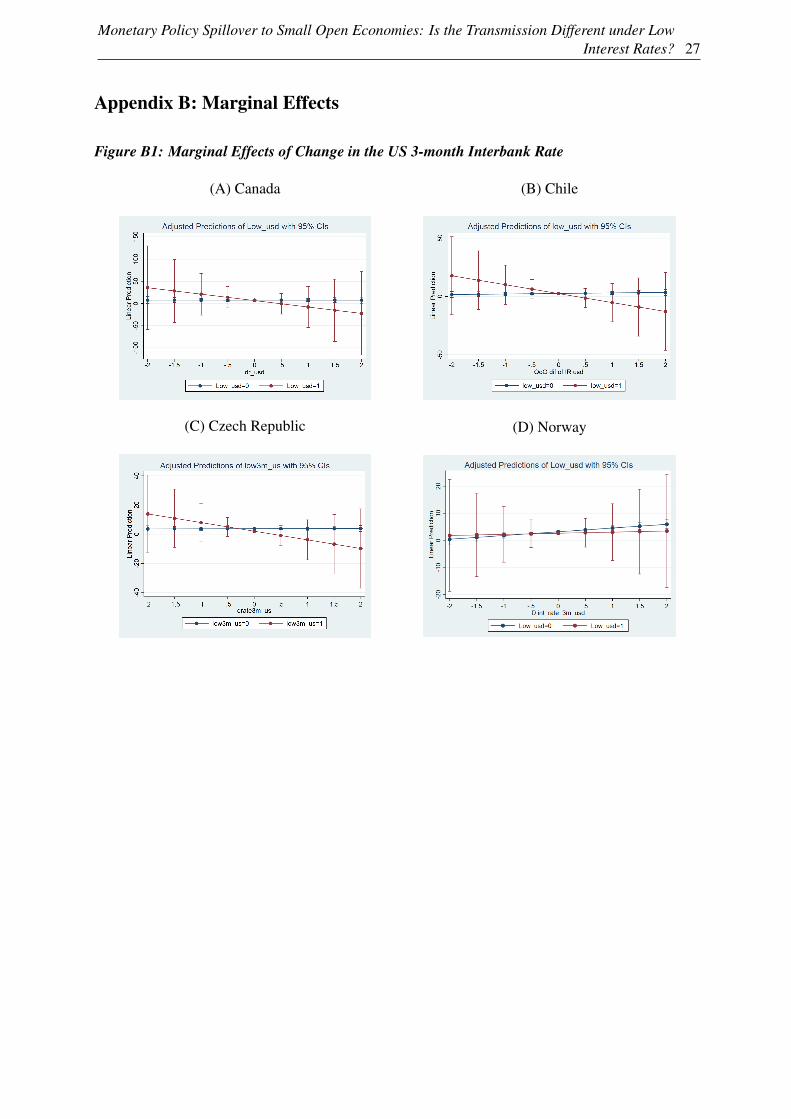
Monetary Policy Spillover to Small Open Economies: Is the Transmission Different under LowInterest Rates? 27
Appendix B: Marginal Effects
Figure B1: Marginal Effects of Change in the US 3-month Interbank Rate
(A) Canada (B) Chile
(C) Czech Republic (D) Norway
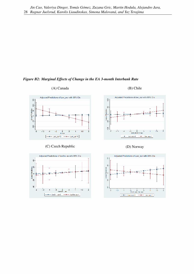
28Jin Cao, Valeriya Dinger, Tomás Gómez, Zuzana Gric, Martin Hodula, Alejandro Jara,Ragnar Juelsrud, Karolis Liaudinskas, Simona Malovaná, and Yaz Terajima
Figure B2: Marginal Effects of Change in the EA 3-month Interbank Rate
(A) Canada (B) Chile
(C) Czech Republic (D) Norway

Monetary Policy Spillover to Small Open Economies: Is the Transmission Different under LowInterest Rates? 29
Figure B3: Marginal Effects of Change in the UK 3-month Interbank Rate
(A) Canada (B) Chile
(C) Czech Republic (D) Norway

30Jin Cao, Valeriya Dinger, Tomás Gómez, Zuzana Gric, Martin Hodula, Alejandro Jara,Ragnar Juelsrud, Karolis Liaudinskas, Simona Malovaná, and Yaz Terajima
Appendix C: Full Regression Results

Monetary Policy Spillover to Small Open Economies: Is the Transmission Different under LowInterest Rates? 31
Tabl
eC
1:B
asel
ine
Res
ults
LH
S:Q
oQL
oan
Gro
wth
Can
ada
Chi
leC
zech
Rep
ublic
Nor
way
US
EA
UK
US
EA
UK
US
EA
UK
SEU
SE
AU
K∆
rc t2.
96**
3.71
*4.
44**
0.47
2.18
***
1.36
**0.
061.
82**
*0.
832.
68**
*1.
38**
*4.
11**
*2.
75**
*(1
.46)
(1.9
8)(1
.95)
(0.6
8)(0
.56)
(0.6
2)(0
.47)
(0.5
9)(0
.56)
(0.3
8)(0
.43)
(0.5
0)(0
.46)
∆Sp
read
c t1.
980.
542.
07-0
.16
0.54
-0.8
3***
0.03
1.35
***
0.63
1.32
***
0.32
1.22
***
1.71
***
(1.3
3)(1
.57)
(1.5
7)(0
.28)
(0.4
4)(0
.26)
(0.4
5)(0
.50)
(0.5
7)(0
.35)
(0.3
0)(0
.42)
(0.4
0)Lo
wc t
0.58
-1.1
5-1
.43*
-0.5
7-0
.01
-0.3
0-1
.70*
**-1
.45*
**-1
.93*
**-2
.90*
**-0
.54*
*-2
.70*
**-1
.42*
**(0
.83)
(1.0
2)(0
.73)
(0.6
8)(0
.59)
(0.7
7)(0
.31)
(0.3
8)(0
.29)
(0.3
0)(0
.26)
(0.3
2)(0
.25)
∆rc t∗L
owc t
-38.
69*
-19.
04-1
0.10
-8.1
310
.16
-1.6
7-5
.98
1.55
-3.8
3-7
.26*
**-0
.97
-7.6
3-5
.70*
*(2
1.94
)(1
4.38
)(1
0.22
)(8
.60)
(12.
26)
(2.9
7)(6
.58)
(7.5
0)(3
.02)
(2.2
7)(5
.31)
(6.8
8)(2
.62)
∆Sp
read
c t∗L
owc t
-3.9
3-2
.71
-2.1
2-0
.51
-0.7
50.
210.
13-2
.46*
*0.
08-1
.28
0.03
-0.2
8-1
.55*
*(2
.42)
(2.3
1)(2
.50)
(1.0
5)(0
.91)
(0.9
5)(1
.00)
(1.1
1)(0
.95)
(0.9
2)(0
.83)
(0.9
4)(0
.68)
Dep
.to
liab.
t−1
18.6
0***
17.6
1**
15.1
1**
8.08
***
8.37
***
8.11
***
-6.4
0***
-6.7
7***
-5.7
9***
-1.4
6-4
.18*
*-1
.57
-4.0
5**
(7.1
7)(7
.79)
(7.6
2)(1
.63)
(1.6
9)(1
.63)
(1.3
7)(1
.36)
(1.3
8)(2
.05)
(2.0
7)(2
.04)
(2.0
5)E
quity
toas
sets
t−1
-166
.10*
**-1
29.5
0*-1
25.4
0*13
.11
13.9
714
.18
10.2
4***
8.94
***
10.3
7***
60.8
1***
57.9
3***
60.0
6***
57.9
8***
(60.
23)
(77.
32)
(64.
23)
(13.
48)
(13.
91)
(13.
71)
(2.9
4)(2
.93)
(2.9
2)(5
.08)
(5.1
9)(5
.04)
(5.1
2)Se
c.to
asse
tst−
10.
75-2
.77
-2.6
5-
--
12.1
2***
9.58
***
10.9
3***
0.08
-3.3
81.
67-1
.51
(10.
38)
(10.
46)
(10.
56)
--
-(1
.23)
(1.3
3)(1
.22)
(3.0
5)(3
.21)
(3.0
6)(3
.13)
Liq
.ass
ets
ratio
t−1
17.3
48.
346.
2317
.76*
**20
.54*
**18
.32*
**8.
89**
*7.
67**
*8.
61**
*33
.08*
**33
.20*
**33
.72*
**33
.52*
**(1
7.59
)(1
7.12
)(1
6.77
)(4
.21)
(4.3
9)(4
.33)
(1.2
9)(1
.40)
(1.2
9)(3
.92)
(3.9
7)(3
.93)
(3.9
5)D
umm
yM
&A
s-
--
40.3
3***
40.4
9***
40.3
1***
--
--
--
--
--
(11.
24)
(11.
22)
(11.
22)
--
--
--
-A
ccou
ntin
gdu
mm
y67
.55*
**66
.44*
**66
.49*
**-
--
--
--
--
-(1
0.92
)(1
0.95
)(1
0.98
)-
--
--
--
--
-Q
oQG
DP
grow
tht−
1-0
.06
-0.0
9-0
.04
0.33
0.07
0.04
0.57
***
0.68
***
0.67
***
-0.0
3-0
.07*
-0.0
6-0
.04
(0.2
3)(0
.24)
(0.2
3)(0
.21)
(0.2
4)(0
.26)
(0.1
6)(0
.18)
(0.1
6)(0
.04)
(0.0
4)(0
.04)
(0.0
4)Q
oQC
PIgr
owth
t−1
0.26
0.03
0.02
0.18
0.09
0.20
0.38
**0.
44**
*0.
43**
*0.
63**
*-0
.06
0.66
***
0.19
(0.2
8)(0
.28)
(0.2
8)(0
.24)
(0.2
4)(0
.23)
(0.1
7)(0
.17)
(0.1
6)(0
.16)
(0.1
6)(0
.16)
(0.1
6)N
648
648
648
885
885
885
1,27
41,
274
1,27
48,
904
8,90
48,
904
8,90
4N
o.of
bank
s9
99
1515
1521
2121
226
226
226
226
R2
0.43
00.
430
0.43
10.
460
0.46
00.
460
0.18
50.
186
0.19
40.
285
0.27
40.
287
0.27
8A
djus
ted
R2
0.41
20.
411
0.41
30.
440
0.45
00.
440
0.16
50.
166
0.17
30.
266
0.25
40.
268
0.25
8FE
Ban
kB
ank
Ban
kB
ank
Ban
kB
ank
Ban
kB
ank
Ban
kB
ank
Ban
kB
ank
Ban
k

32Jin Cao, Valeriya Dinger, Tomás Gómez, Zuzana Gric, Martin Hodula, Alejandro Jara,Ragnar Juelsrud, Karolis Liaudinskas, Simona Malovaná, and Yaz Terajima
Tabl
eC
2:Th
eR
ole
ofIn
tern
atio
nalB
anks
LH
S:Q
oQL
oan
Gro
wth
Can
ada
Chi
leC
zech
Rep
ublic
Nor
way
US
EA
UK
US
EA
UK
US
EA
UK
SEU
SE
AU
K∆
rc t2.
96**
3.71
*8.
720.
082.
95**
*1.
62**
0.02
2.98
0.84
2.02
***
1.47
***
3.39
***
2.42
***
(1.4
6)(1
.98)
(6.5
5)(0
.59)
(0.7
6)(0
.59)
(0.5
3)(1
.88)
(0.6
5)(0
.34)
(0.3
8)(0
.40)
(0.4
3)∆
Spre
adc t
1.98
0.54
6.37
0.40
1.11
**0.
070.
043.
02*
0.68
0.96
***
0.45
1.28
***
1.57
***
(1.3
3)(1
.57)
(9.2
3)(0
.49)
(0.4
7)(0
.72)
(0.5
1)(1
.63)
(0.6
8)(0
.31)
(0.2
8)(0
.33)
(0.3
7)∆
rc t∗L
owc t
0.58
-1.1
5-1
.44*
*-1
3.29
15.3
9-0
.94
-4.5
4-3
7.56
*-3
.43
-4.1
1**
-2.7
2-8
.25*
-1.4
0(0
.83)
(1.0
2)(0
.74)
(16.
52)
(10.
54)
(3.6
4)(7
.43)
(21.
50)
(3.6
1)(1
.68)
(3.8
3)(4
.98)
(1.8
7)∆
Spre
adc t∗L
owc t
-38.
69*
-19.
0417
.97
-3.5
4***
-2.9
8***
-0.9
80.
41-6
.39*
*-1
.02
-0.7
3-0
.36
-0.5
0-1
.74*
**(2
1.94
)(1
4.38
)(1
5.66
)(0
.74)
(0.9
1)(1
.00)
(1.1
3)(3
.20)
(1.1
3)(0
.71)
(0.6
1)(0
.69)
(0.5
3)Lo
wc t
-3.9
3-2
.71
-8.1
7-1
.30*
*0.
51-1
.17*
**-1
.57*
**0.
18-2
.10*
**-2
.39*
**-0
.75*
**-2
.40*
**-1
.19*
**(2
.42)
(2.3
1)(1
0.06
)(0
.52)
(0.4
5)(0
.32)
(0.3
5)(1
.09)
(0.3
5)(0
.23)
(0.2
1)(0
.25)
(0.2
0)Lo
wc t∗F
amil
yc t-
--
--
--0
.63
-1.6
70.
53-4
.59*
**2.
44-2
.50
-2.6
1-
--
--
-(0
.72)
(1.0
9)(0
.62)
(1.6
0)(2
.21)
(1.8
2)(1
.85)
∆rc t∗F
amil
yc t-
--4
.83
0.76
-1.8
6-0
.80
0.20
-1.2
4-0
.02
7.01
***
-1.2
57.
16**
3.76
--
(7.2
2)(1
.30)
(1.2
3)(0
.92)
(1.0
7)(1
.94)
(1.1
4)(2
.27)
(3.5
8)(3
.01)
(2.8
0)∆
Spre
adc t∗F
amil
yc t-
--4
.83
-1.7
1-2
.75*
**-1
.21
-0.0
3-1
.87
-0.1
53.
65*
-1.6
8-0
.74
1.65
--
(10.
21)
(1.0
5)(0
.90)
(1.1
2)(1
.03)
(1.7
1)(1
.23)
(2.1
9)(2
.07)
(2.8
6)(2
.59)
∆rc t∗L
owc t∗F
amil
yc t-
--3
1.63
9.64
-13.
19-1
.91
-6.7
644
.72*
*-1
.18
-26.
72*
22.0
94.
65-4
9.70
**-
-(1
9.76
)(1
7.40
)(3
0.93
)(4
.97)
(15.
63)
(22.
62)
(6.4
8)(1
4.25
)(4
7.71
)(4
4.48
)(2
1.79
)∆
Spre
adc t∗L
owc t∗F
amil
yc t-
-6.
795.
26**
*5.
46**
*3.
57**
*-1
.31
4.49
3.50
*-5
.24
4.85
2.07
1.91
--
(11.
12)
(1.5
6)(1
.25)
(1.1
5)(2
.39)
(3.3
8)(2
.03)
(5.5
4)(7
.19)
(6.1
6)(5
.56)
Dep
.to
liab.
t−1
18.6
0***
17.6
1**
15.3
7**
8.61
***
8.92
***
8.81
***
-6.4
0***
-7.7
1***
-5.6
8***
-1.4
0-4
.23*
*-1
.66
-3.8
5*(7
.17)
(7.7
9)(7
.71)
(1.8
8)(1
.93)
(1.8
9)(1
.37)
(1.3
9)(1
.39)
(2.0
4)(2
.07)
(2.0
3)(2
.04)
Equ
ityto
asse
tst−
1-1
66.1
0***
-129
.50*
-120
.40*
16.8
3***
15.7
6**
15.7
8**
10.6
4***
8.59
***
10.1
8***
60.6
7***
57.6
3***
59.6
7***
58.0
6***
(60.
23)
(77.
32)
(65.
75)
(5.2
9)(5
.98)
(5.5
4)(2
.97)
(2.9
1)(2
.92)
(5.0
4)(5
.24)
(5.0
0)(5
.12)
Sec.
toas
sets
t−1
0.75
-2.7
7-2
.30
--
-12
.17*
**9.
89**
*10
.78*
**-0
.44
-3.1
91.
02-1
.94
(10.
38)
(10.
46)
(10.
66)
--
-(1
.23)
(1.3
3)(1
.23)
(3.0
1)(3
.23)
(2.9
9)(3
.13)
Liq
.ass
ets
ratio
t−1
17.3
48.
347.
0619
.10*
*21
.45*
**19
.07*
*8.
76**
*8.
07**
*8.
79**
*34
.10*
**33
.16*
**34
.66*
**33
.61*
**(1
7.59
)(1
7.12
)(1
7.30
)(6
.75)
(5.6
2)(6
.64)
(1.3
0)(1
.41)
(1.3
1)(3
.83)
(3.9
5)(3
.84)
(3.9
3)D
umm
yM
&A
s-
--
40.6
0***
40.3
6***
40.2
9***
--
--
--
--
--
(12.
58)
(12.
61)
(12.
71)
--
--
--
-A
ccou
ntin
gdu
mm
y67
.55*
**66
.44*
**66
.48*
**-
--
--
--
--
-(1
0.92
)(1
0.95
)(1
0.88
)-
--
--
--
--
-Q
oQG
DP
grow
tht−
1-0
.06
-0.0
9-0
.04
0.32
0.07
0.03
0.57
***
0.65
***
0.67
***
-0.0
3-0
.07*
-0.0
5-0
.04
(0.2
3)(0
.24)
(0.2
4)(0
.23)
(0.2
1)(0
.27)
(0.1
6)(0
.18)
(0.1
6)(0
.04)
(0.0
4)(0
.04)
(0.0
4)Q
oQC
PIgr
owth
t−1
0.26
0.03
0.02
0.19
0.10
0.20
0.38
**0.
42**
0.43
***
0.63
***
-0.0
50.
67**
*0.
19(0
.28)
(0.2
8)(0
.28)
(0.2
5)(0
.27)
(0.2
4)(0
.17)
(0.1
7)(0
.16)
(0.1
6)(0
.16)
(0.1
6)(0
.16)
N64
864
864
888
588
588
51,
274
1,27
41,
274
8,90
48,
904
8,90
48,
904
No.
ofba
nks
99
915
1515
2121
2122
622
722
822
9R
20.
430
0.43
00.
434
0.47
00.
470
0.46
00.
186
0.19
70.
197
0.29
00.
274
0.29
20.
282
Adj
uste
dR
20.
412
0.41
10.
412
0.45
00.
450
0.44
00.
162
0.17
40.
174
0.27
10.
254
0.27
20.
262
FEB
ank
Ban
kB
ank
Ban
kB
ank
Ban
kB
ank
Ban
kB
ank
Ban
kB
ank
Ban
kB
ank

Monetary Policy Spillover to Small Open Economies: Is the Transmission Different under LowInterest Rates? 33
Tabl
eC
3:Sp
illov
ersA
cros
sLoa
nC
ateg
orie
s–M
ortg
age
Lend
ing
LH
S:Q
oQM
ortg
age
Loa
nG
row
thC
anad
aC
hile
Cze
chR
epub
licN
orw
ayU
SE
AU
KU
SE
AU
KU
SE
AU
KSE
US
EA
UK
∆rc t
4.59
**5.
98**
*8.
22**
*-0
.63
0.61
0.21
0.29
1.69
**0.
851.
57**
*-0
.14
2.76
***
1.87
***
(1.8
3)(2
.21)
(2.1
6)(0
.76)
(0.7
6)(0
.82)
(0.6
8)(0
.86)
(0.8
1)(0
.39)
(0.4
2)(0
.43)
(0.4
6)∆
Spre
adc t
2.58
0.09
3.60
*-0
.49
0.52
0.01
-0.1
51.
32*
0.63
0.44
-0.3
80.
530.
29(1
.67)
(1.9
3)(2
.11)
(0.7
7)(0
.76)
(0.9
8)(0
.66)
(0.7
3)(0
.83)
(0.3
1)(0
.27)
(0.3
4)(0
.36)
Low
c t2.
44**
*-2
.77*
-0.9
9-0
.21
-0.4
1-0
.69*
*-1
.45*
**-2
.31*
**-1
.68*
**-1
.88*
**-0
.62*
**-1
.86*
**-0
.70*
**(0
.92)
(1.4
8)(0
.86)
(0.3
6)(0
.55)
(0.3
0)(0
.46)
(0.5
5)(0
.44)
(0.2
3)(0
.21)
(0.2
5)(0
.21)
∆rc t∗L
owc t
-60.
37*
-46.
83**
*-2
4.66
*-2
5.44
**2.
26-2
.00
-5.4
2-2
.55
-1.5
5-4
.87*
*2.
83-6
.94
-1.2
8(3
1.32
)(1
6.81
)(1
4.62
)(1
1.14
)(1
2.61
)(2
.59)
(9.5
9)(1
0.93
)(4
.44)
(1.9
5)(3
.96)
(5.6
0)(1
.98)
∆Sp
read
c t∗L
owc t
-5.4
3**
-0.7
2-2
.99
0.23
-1.4
90.
651.
38-1
.72
0.05
-1.8
0**
0.85
-1.3
6*-0
.75
(2.5
8)(2
.54)
(2.8
0)(1
.68)
(1.1
3)(1
.15)
(1.4
6)(1
.61)
(1.3
9)(0
.81)
(0.6
5)(0
.79)
(0.5
8)D
ep.t
olia
b.t−
126
.26*
**21
.61*
*20
.53*
*0.
060.
100.
88-1
6.28
***
-15.
81**
*-1
5.57
***
0.15
-1.8
50.
07-2
.15
(8.6
6)(1
0.01
)(9
.46)
(2.4
2)(2
.66)
(2.4
2)(1
.98)
(1.9
6)(2
.01)
(1.7
6)(1
.79)
(1.7
6)(1
.78)
Equ
ityto
asse
tst−
1-8
2.84
21.7
2-2
2.72
1.96
2.13
2.60
-3.8
2-4
.96
-3.3
846
.85*
**44
.26*
**46
.15*
**43
.97*
**(7
9.23
)(1
15.4
0)(9
3.90
)(1
2.54
)(1
3.20
)(1
3.01
)(4
.38)
(4.3
3)(4
.36)
(5.3
5)(5
.45)
(5.3
0)(5
.36)
Sec.
toas
sets
t−1
14.2
68.
0110
.52
--
-14
.21*
**10
.79*
**13
.28*
**-1
3.00
***
-15.
44**
*-1
1.28
***
-14.
90**
*(1
3.30
)(1
3.31
)(1
3.71
)-
--
(1.8
0)(1
.94)
(1.8
1)(2
.53)
(2.6
4)(2
.57)
(2.5
8)L
iq.a
sset
sra
tiot−
135
.27
18.7
516
.16
12.5
7**
12.3
5**
12.4
8**
10.1
6***
7.67
***
10.0
6***
24.6
5***
25.5
4***
25.3
0***
25.9
6***
(23.
94)
(22.
76)
(22.
20)
(5.3
4)(5
.89)
(5.5
5)(1
.88)
(2.0
2)(1
.89)
(3.1
9)(3
.24)
(3.1
9)(3
.23)
Dum
my
M&
As
--
-33
.72*
**34
.05*
**33
.86*
**-
--
--
--
--
-(1
0.35
)(1
0.43
)(1
0.39
)-
--
--
--
Acc
ount
ing
dum
my
102.
60**
*10
0.20
***
101.
10**
*-
--
--
--
--
-(1
7.72
)(1
7.79
)(1
7.82
)-
--
--
--
--
-Q
oQG
DP
grow
tht−
1-0
.54*
-0.5
8*-0
.54*
0.45
*0.
430.
390.
46**
0.71
***
0.57
**-0
.02
-0.0
3-0
.03
-0.0
4(0
.30)
(0.3
1)(0
.30)
(0.2
6)(0
.28)
(0.3
1)(0
.23)
(0.2
6)(0
.23)
(0.0
4)(0
.04)
(0.0
4)(0
.04)
QoQ
CPI
grow
tht−
10.
31-0
.07
-0.0
30.
250.
280.
250.
370.
380.
360.
30**
-0.1
70.
40**
*0.
17(0
.36)
(0.3
4)(0
.33)
(0.2
6)(0
.26)
(0.2
6)(0
.25)
(0.2
4)(0
.24)
(0.1
4)(0
.14)
(0.1
4)(0
.13)
N64
864
864
882
882
882
81,
229
1,22
91,
229
8,13
48,
134
8,13
48,
134
No.
ofba
nks
99
914
1414
2121
2122
622
622
622
6R
20.
480
0.47
90.
482
0.41
00.
400
0.40
00.
240
0.15
20.
163
0.22
70.
220
0.22
90.
222
Adj
uste
dR
20.
464
0.46
20.
466
0.39
00.
390
0.39
00.
215
0.13
00.
141
0.20
70.
200
0.20
90.
202
FEB
ank
Ban
kB
ank
Ban
kB
ank
Ban
kB
ank
Ban
kB
ank
Ban
kB
ank
Ban
kB
ank

34Jin Cao, Valeriya Dinger, Tomás Gómez, Zuzana Gric, Martin Hodula, Alejandro Jara,Ragnar Juelsrud, Karolis Liaudinskas, Simona Malovaná, and Yaz Terajima
Tabl
eC
4:Sp
illov
ersA
cros
sLoa
nC
ateg
orie
s–C
onsu
mer
Lend
ing
LH
S:Q
oQC
onsu
mer
Loa
nG
row
thC
anad
aC
hile
Cze
chR
epub
licN
orw
ayU
SE
AU
KU
SE
AU
KU
SE
AU
KSE
US
EA
UK
∆rc t
-1.6
91.
820.
90-0
.19
4.19
***
2.43
*4.
08**
5.24
**3.
120.
069.
35**
*2.
13*
1.59
(1.8
1)(2
.39)
(2.1
8)(0
.87)
(1.2
0)(1
.41)
(2.0
3)(2
.56)
(2.4
4)(1
.08)
(1.4
5)(1
.22)
(1.1
9)∆
Spre
adc t
2.21
3.25
3.12
-0.8
22.
00*
0.44
0.75
1.53
1.86
0.41
0.97
0.55
2.34
**(1
.60)
(1.9
9)(2
.14)
(0.9
7)(1
.13)
(1.4
9)(1
.99)
(2.1
7)(2
.53)
(0.9
3)(0
.79)
(1.0
0)(1
.11)
Low
c t-3
.09*
**-5
.10*
**-5
.40*
**-0
.68
-2.4
3***
-2.2
6***
-0.0
4-4
.33*
*0.
67-2
.59*
**0.
46-2
.40*
**-0
.62
(1.0
2)(1
.15)
(0.9
0)(0
.53)
(0.8
4)(0
.49)
(1.5
0)(1
.69)
(1.3
4)(0
.68)
(0.5
8)(0
.74)
(0.5
8)∆
rc t∗L
owc t
-16.
0614
.72
-2.0
3-4
.11
-1.9
5-5
.11*
-30.
71-1
6.05
5.87
-11.
31**
-4.0
8-2
3.36
-14.
31**
*(2
2.84
)(1
3.44
)(1
2.52
)(1
3.77
)(1
2.30
)(3
.01)
(28.
42)
(32.
30)
(13.
13)
(5.3
8)(1
1.71
)(1
6.58
)(5
.50)
∆Sp
read
c t∗L
owc t
-2.3
5-4
.83*
-3.1
81.
85-2
.55*
-1.0
8-0
.48
-5.6
5-0
.78
0.41
2.37
6.67
***
-1.1
0(2
.93)
(2.8
1)(2
.76)
(2.5
8)(1
.30)
(1.5
3)(4
.30)
(4.7
6)(4
.11)
(2.3
5)(1
.88)
(2.3
0)(1
.62)
Dep
.to
liab.
t−1
25.8
5**
19.4
6*20
.65*
*-1
1.08
**-1
6.67
***
-10.
22**
-17.
14**
*-1
3.49
***
-17.
36**
*-3
.19
-8.2
5**
-3.0
3-5
.13
(10.
28)
(10.
06)
(10.
31)
(4.8
5)(5
.49)
(4.6
8)(5
.16)
(5.1
8)(5
.26)
(3.4
6)(3
.45)
(3.4
6)(3
.46)
Equ
ityto
asse
tst−
1-5
62.1
0***
-462
.80*
**-5
13.2
0***
-27.
33**
-25.
92*
-25.
64*
20.6
615
.22
20.0
960
.38*
**53
.83*
**59
.54*
**57
.72*
**(7
5.15
)(8
5.04
)(7
4.37
)(1
3.73
)(1
4.20
)(1
3.95
)(1
8.95
)(1
8.97
)(1
8.95
)(1
0.90
)(1
0.88
)(1
0.83
)(1
0.90
)Se
c.to
asse
tst−
1-1
7.39
-25.
02*
-25.
69**
--
-12
.92
7.86
12.4
10.
64-0
.71
1.83
-1.1
9(1
2.16
)(1
2.91
)(1
2.25
)-
--
(8.7
4)(8
.30)
(8.2
3)(5
.79)
(6.0
6)(5
.81)
(5.9
9)L
iq.a
sset
sra
tiot−
17.
1116
.40
2.00
-1.9
4-5
.55
-2.9
59.
03*
4.45
10.4
6**
22.0
6***
23.7
6***
22.9
9***
22.1
6***
(16.
75)
(17.
17)
(16.
81)
(8.6
1)(9
.09)
(8.5
8)(4
.94)
(5.5
5)(5
.05)
(6.5
3)(6
.56)
(6.5
2)(6
.57)
Dum
my
M&
As
--
-35
.30*
**35
.78*
**35
.19*
**-
--
--
--
--
-(1
0.24
)(1
0.27
)(1
0.12
)-
--
--
--
Acc
ount
ing
dum
my
20.6
7***
19.9
0***
20.4
5***
--
--
--
--
--
(6.3
8)(6
.36)
(6.4
6)-
--
--
--
--
-Q
oQG
DP
grow
tht−
10.
03-0
.28
0.03
0.76
**0.
210.
260.
00-0
.06
0.02
-0.1
5-0
.39*
**-0
.16
-0.1
4(0
.22)
(0.2
3)(0
.22)
(0.3
6)(0
.42)
(0.4
6)(0
.70)
(0.7
9)(0
.72)
(0.1
2)(0
.13)
(0.1
2)(0
.12)
QoQ
CPI
grow
tht−
10.
420.
380.
09-1
.05*
**-0
.97*
*-1
.03*
**0.
990.
390.
690.
17-0
.10
0.31
-0.0
9(0
.32)
(0.3
2)(0
.32)
(0.3
8)(0
.39)
(0.3
7)(0
.74)
(0.7
4)(0
.72)
(0.4
2)(0
.40)
(0.4
0)(0
.40)
N64
864
864
882
882
882
891
091
091
08,
128
8,12
88,
128
8,12
8N
o.of
bank
s9
99
1414
1418
1818
226
226
226
226
R2
0.23
40.
246
0.24
70.
240
0.26
00.
260
0.03
20.
040
0.02
70.
054
0.06
00.
055
0.05
4A
djus
ted
R2
0.20
90.
222
0.22
30.
220
0.24
00.
230
0.00
10.
010
-0.0
040.
028
0.03
40.
029
0.02
8FE
Ban
kB
ank
Ban
kB
ank
Ban
kB
ank
Ban
kB
ank
Ban
kB
ank
Ban
kB
ank
Ban
k

Monetary Policy Spillover to Small Open Economies: Is the Transmission Different under LowInterest Rates? 35
Tabl
eC
5:Sp
illov
ersA
cros
sLoa
nC
ateg
orie
s–C
orpo
rate
Lend
ing
LH
S:Q
oQC
orpo
rate
Loa
nG
row
th Can
ada
Chi
leC
zech
Rep
ublic
Nor
way
US
EA
UK
US
EA
UK
US
EA
UK
SEU
SE
AU
K∆
rc t3.
536.
20**
1.67
0.42
1.53
**1.
022.
04**
2.95
**2.
85**
2.28
***
0.05
3.46
***
1.80
***
(2.4
5)(3
.11)
(2.9
5)(0
.75)
(0.6
3)(0
.68)
(0.9
4)(1
.19)
(1.1
2)(0
.51)
(0.6
0)(0
.64)
(0.6
4)∆
Spre
adc t
1.64
2.87
-3.1
6-0
.59
-0.5
7-1
.04
0.82
2.06
**1.
061.
12**
0.16
1.61
***
1.08
*(2
.71)
(2.7
3)(3
.06)
(0.7
2)(0
.66)
(0.8
4)(0
.92)
(1.0
0)(1
.16)
(0.4
8)(0
.41)
(0.5
3)(0
.56)
Low
c t0.
574.
51**
2.63
-0.1
80.
60-0
.89*
**-1
.10*
-3.1
7***
-2.0
5***
-2.3
8***
-1.0
2***
-2.4
1***
-1.7
2***
(1.8
1)(2
.17)
(1.8
5)(0
.41)
(0.5
0)(0
.31)
(0.6
3)(0
.75)
(0.5
9)(0
.40)
(0.3
3)(0
.44)
(0.3
3)∆
rc t∗L
owc t
-19.
243.
0519
.53
-24.
83*
7.24
-2.2
6-8
.48
-1.2
7-7
.40
-5.3
5*-1
.20
-10.
06-0
.64
(38.
13)
(45.
51)
(20.
18)
(14.
52)
(13.
29)
(3.4
5)(1
3.22
)(1
4.97
)(6
.08)
(2.9
4)(6
.90)
(8.3
8)(3
.05)
∆Sp
read
c t∗L
owc t
-0.6
0-6
.67
5.50
-1.1
40.
372.
08*
1.28
-2.3
50.
89-1
.14
0.16
-1.1
0-0
.79
(5.4
1)(6
.96)
(5.9
0)(1
.31)
(1.1
3)(1
.10)
(2.0
1)(2
.21)
(1.9
0)(1
.25)
(1.0
4)(1
.19)
(0.8
9)D
ep.t
olia
b.t−
113
.06
20.8
317
.12
8.75
***
9.56
***
9.10
***
-11.
70**
*-9
.81*
**-1
0.61
***
-3.0
0-5
.10
-2.9
7-4
.85
(16.
19)
(16.
23)
(16.
19)
(1.7
0)(1
.76)
(1.6
9)(2
.76)
(2.7
2)(2
.78)
(3.9
1)(3
.85)
(3.9
0)(3
.87)
Equ
ityto
asse
tst−
120
.24
-102
.20
-25.
2217
.20
18.4
719
.11
16.5
9**
15.7
2*18
.32*
*35
.28*
**30
.81*
**34
.76*
**31
.41*
**(1
03.6
0)(1
14.8
0)(1
04.0
0)(2
4.16
)(2
4.89
)(2
4.64
)(8
.39)
(8.2
7)(8
.35)
(9.5
5)(9
.71)
(9.5
2)(9
.63)
Sec.
toas
sets
t−1
-55.
42**
*-5
5.70
***
-52.
42**
*-
--
17.4
9***
12.7
0***
16.4
1***
-15.
88**
*-1
8.59
***
-14.
25**
*-1
6.63
***
(18.
29)
(18.
37)
(18.
16)
--
-(2
.48)
(2.6
7)(2
.47)
(3.9
9)(4
.13)
(4.0
4)(4
.07)
Liq
.ass
ets
ratio
t−1
-31.
70-5
1.39
*-3
6.23
14.3
9***
18.0
2***
15.7
7***
4.69
*1.
224.
61*
24.2
2***
24.1
3***
24.7
3***
24.5
3***
(28.
84)
(28.
58)
(28.
36)
(4.8
1)(5
.21)
(5.1
2)(2
.60)
(2.8
0)(2
.61)
(6.6
5)(6
.68)
(6.6
4)(6
.65)
Dum
my
M&
As
--
-46
.21*
**46
.38*
**46
.25*
**-
--
--
--
--
-(1
3.88
)(1
3.94
)(1
3.94
)-
--
--
--
Acc
ount
ing
dum
my
0.82
1.49
-0.7
4-
--
--
--
--
-(6
.89)
(6.8
8)(7
.01)
--
--
--
--
--
QoQ
GD
Pgr
owth
t−1
0.91
**0.
94**
0.67
*0.
06-0
.13
-0.2
80.
86**
*1.
16**
*0.
75**
-0.0
8-0
.09
-0.0
9-0
.08
(0.4
1)(0
.40)
(0.4
0)(0
.25)
(0.2
8)(0
.30)
(0.3
2)(0
.36)
(0.3
2)(0
.06)
(0.0
6)(0
.06)
(0.0
6)Q
oQC
PIgr
owth
t−1
-0.1
7-0
.35
-0.2
40.
250.
100.
200.
95**
*0.
81**
0.76
**0.
83**
*0.
230.
84**
*0.
48**
(0.4
9)(0
.49)
(0.5
0)(0
.27)
(0.2
8)(0
.27)
(0.3
4)(0
.34)
(0.3
3)(0
.23)
(0.2
1)(0
.22)
(0.2
2)N
648
648
648
885
885
885
1,26
01,
260
1,26
08,
417
8,41
78,
417
8,41
7N
o.of
bank
s9
99
1515
1521
2121
226
226
226
226
R2
0.05
10.
064
0.05
80.
430
0.43
00.
430
0.08
70.
103
0.09
50.
125
0.12
00.
126
0.12
3A
djus
ted
R2
0.02
00.
034
0.02
80.
410
0.41
00.
420
0.06
40.
080
0.07
20.
102
0.09
60.
103
0.09
9FE
Ban
kB
ank
Ban
kB
ank
Ban
kB
ank
Ban
kB
ank
Ban
kB
ank
Ban
kB
ank
Ban
k

36Jin Cao, Valeriya Dinger, Tomás Gómez, Zuzana Gric, Martin Hodula, Alejandro Jara,Ragnar Juelsrud, Karolis Liaudinskas, Simona Malovaná, and Yaz Terajima
Tabl
eC
6:A
ltern
ativ
eM
onet
ary
Polic
yIn
dica
tor–
Shad
owR
ate
LH
S:Q
oQL
oan
Gro
wth
Can
ada
Chi
leC
zech
Rep
ublic
Nor
way
US
EA
UK
US
EA
UK
US
EA
UK
SEU
SE
AU
K∆
shad
owc t
1.89
*3.
21**
0.82
0.46
0.68
*0.
30-0
.69*
*0.
470.
321.
71**
*0.
042.
07**
*0.
62**
*(1
.03)
(1.4
0)(0
.88)
(0.6
2)(0
.41)
(0.2
1)(0
.35)
(0.3
3)(0
.19)
(0.2
9)(0
.30)
(0.3
9)(0
.15)
Low
c t1.
14-0
.90
-0.9
9-0
.15
0.57
-0.6
8**
-1.6
4***
-1.8
3***
-1.8
1***
-2.8
8***
-0.5
6**
-2.3
0***
-1.2
6***
(0.8
7)(1
.05)
(0.7
7)(0
.31)
(0.4
9)(0
.26)
(0.2
9)(0
.34)
(0.2
9)(0
.29)
(0.2
5)(0
.31)
(0.2
5)∆
shad
owc t∗L
owc t
-1.6
4-4
.67*
**-1
.82*
-0.1
1-0
.31
-0.5
0-0
.50
-1.9
3***
-0.6
6-7
.05*
**-0
.04
-2.1
8***
-0.7
2**
(2.3
3)(1
.79)
(1.0
8)(0
.84)
(0.5
5)(0
.35)
(0.8
0)(0
.58)
(0.4
3)(1
.51)
(0.7
1)(0
.51)
(0.3
1)D
ep.t
olia
b.t−
119
.39*
**30
.50*
**15
.74*
*8.
30**
*10
.02*
**7.
91**
*-6
.15*
**-6
.92*
**-5
.81*
**-1
.45
-3.7
8*-3
.47
-3.8
9*(7
.15)
(9.7
3)(7
.47)
(1.6
1)(1
.92)
(1.6
1)(1
.36)
(1.3
5)(1
.37)
(2.0
6)(2
.09)
(2.7
1)(2
.04)
Equ
ityto
asse
tst−
1-1
71.3
0***
-194
.40*
*-1
30.9
0**
13.0
213
.31
13.0
110
.85*
**8.
32**
*10
.39*
**61
.02*
**58
.33*
**61
.28*
**58
.20*
**(5
9.72
)(9
0.58
)(6
2.90
)(1
3.91
)(1
5.03
)(1
3.85
)(2
.93)
(2.9
1)(2
.91)
(5.0
8)(5
.22)
(5.2
5)(5
.13)
Sec.
toas
sets
t−1
2.99
0.93
-0.9
6-
--
12.2
3***
9.19
***
11.1
2***
-0.6
0-3
.69
2.08
-2.5
9(1
0.59
)(1
2.58
)(1
0.67
)-
--
(1.2
2)(1
.30)
(1.2
1)(3
.04)
(3.2
1)(3
.65)
(3.1
1)L
iq.a
sset
sra
tiot−
116
.91
21.2
99.
2018
.42*
**21
.23*
**17
.79*
**8.
97**
*7.
20**
*8.
93**
*32
.93*
**32
.98*
**34
.89*
**33
.25*
**(1
7.47
)(2
0.07
)(1
6.79
)(4
.29)
(5.2
3)(4
.29)
(1.2
8)(1
.36)
(1.2
8)(3
.92)
(3.9
6)(4
.29)
(3.9
5)D
umm
yM
&A
s-
--
40.3
5***
39.5
0***
40.2
0***
--
--
--
--
--
(11.
27)
(13.
74)
(11.
27)
--
--
--
-A
ccou
ntin
gdu
mm
y67
.22*
**69
.21*
**66
.38*
**-
--
--
--
--
-(1
0.90
)(1
1.02
)(1
0.96
)-
--
--
--
--
-Q
oQG
DP
grow
tht−
1-0
.05
-0.1
10.
060.
40*
0.44
*0.
310.
69**
*0.
79**
*0.
61**
*-0
.03
-0.0
5-0
.06
-0.0
5(0
.23)
(0.2
4)(0
.22)
(0.2
0)(0
.25)
(0.2
1)(0
.15)
(0.1
5)(0
.15)
(0.0
4)(0
.04)
(0.0
5)(0
.04)
QoQ
CPI
grow
tht−
10.
160.
040.
140.
310.
52**
0.36
*0.
37**
0.57
***
0.46
***
0.50
***
-0.0
50.
320.
15(0
.27)
(0.3
4)(0
.27)
(0.1
9)(0
.21)
(0.2
1)(0
.17)
(0.1
6)(0
.16)
(0.1
6)(0
.15)
(0.2
1)(0
.15)
N64
854
964
888
573
388
51,
274
1,27
41,
274
8,90
48,
904
7,61
98,
904
No.
ofba
nks
99
915
1515
2121
2122
622
622
622
6R
20.
426
0.46
90.
426
0.45
00.
440
0.45
00.
188
0.18
60.
193
0.28
50.
273
0.29
10.
276
Adj
uste
dR
20.
410
0.45
10.
409
0.44
00.
420
0.44
00.
169
0.16
70.
174
0.26
60.
253
0.27
00.
257
FEB
ank
Ban
kB
ank
Ban
kB
ank
Ban
kB
ank
Ban
kB
ank
Ban
kB
ank
Ban
kB
ank
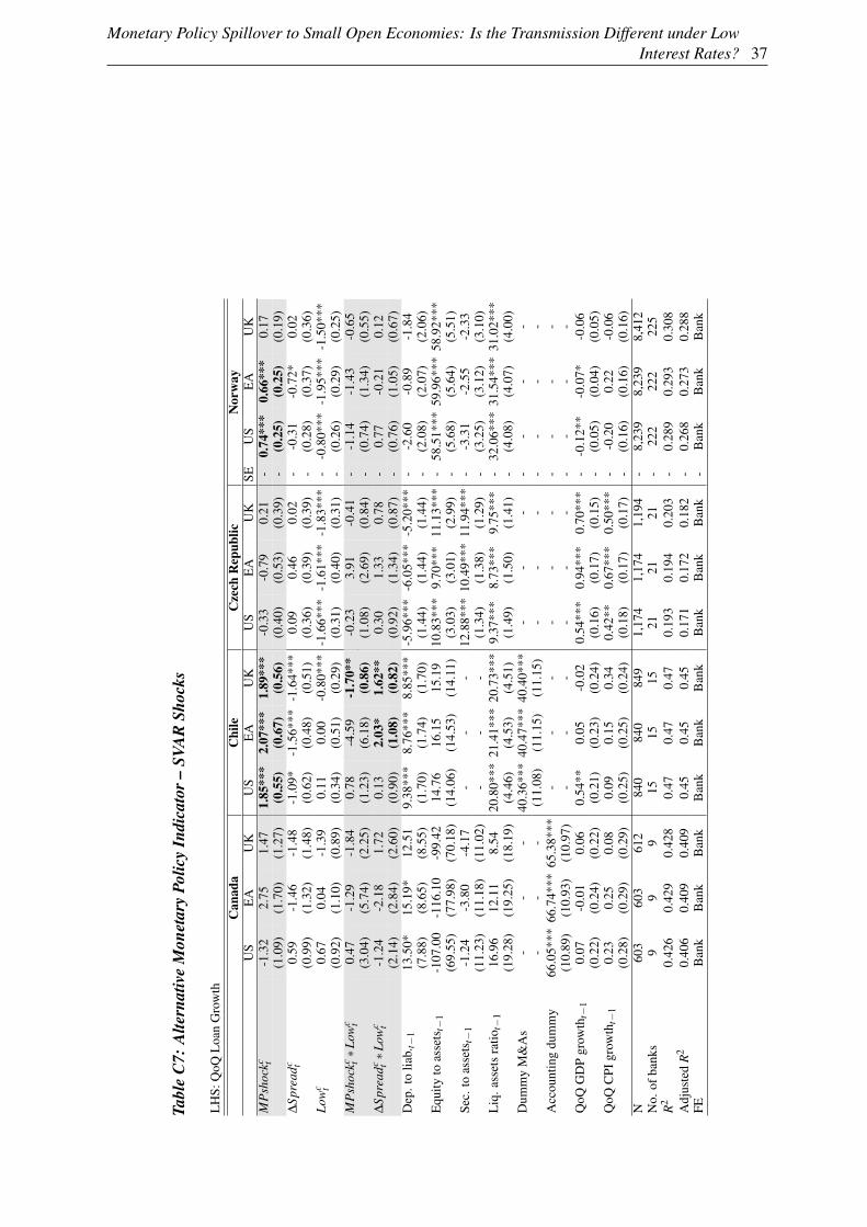
Monetary Policy Spillover to Small Open Economies: Is the Transmission Different under LowInterest Rates? 37
Tabl
eC
7:A
ltern
ativ
eM
onet
ary
Polic
yIn
dica
tor–
SVA
RSh
ocks
LH
S:Q
oQL
oan
Gro
wth
Can
ada
Chi
leC
zech
Rep
ublic
Nor
way
US
EA
UK
US
EA
UK
US
EA
UK
SEU
SE
AU
KM
Psh
ockc t
-1.3
22.
751.
471.
85**
*2.
07**
*1.
89**
*-0
.33
-0.7
90.
21-
0.74
***
0.66
***
0.17
(1.0
9)(1
.70)
(1.2
7)(0
.55)
(0.6
7)(0
.56)
(0.4
0)(0
.53)
(0.3
9)-
(0.2
5)(0
.25)
(0.1
9)∆
Spre
adc t
0.59
-1.4
6-1
.48
-1.0
9*-1
.56*
**-1
.64*
**0.
090.
460.
02-
-0.3
1-0
.72*
0.02
(0.9
9)(1
.32)
(1.4
8)(0
.62)
(0.4
8)(0
.51)
(0.3
6)(0
.39)
(0.3
9)-
(0.2
8)(0
.37)
(0.3
6)Lo
wc t
0.67
0.04
-1.3
90.
110.
00-0
.80*
**-1
.66*
**-1
.61*
**-1
.83*
**-
-0.8
0***
-1.9
5***
-1.5
0***
(0.9
2)(1
.10)
(0.8
9)(0
.34)
(0.5
1)(0
.29)
(0.3
1)(0
.40)
(0.3
1)-
(0.2
6)(0
.29)
(0.2
5)M
Psh
ockc t
∗Low
c t0.
47-1
.29
-1.8
40.
78-4
.59
-1.7
0**
-0.2
33.
91-0
.41
--1
.14
-1.4
3-0
.65
(3.0
4)(5
.74)
(2.2
5)(1
.23)
(6.1
8)(0
.86)
(1.0
8)(2
.69)
(0.8
4)-
(0.7
4)(1
.34)
(0.5
5)∆
Spre
adc t∗L
owc t
-1.2
4-2
.18
1.72
0.13
2.03
*1.
62**
0.30
1.33
0.78
-0.
77-0
.21
0.12
(2.1
4)(2
.84)
(2.6
0)(0
.90)
(1.0
8)(0
.82)
(0.9
2)(1
.34)
(0.8
7)-
(0.7
6)(1
.05)
(0.6
7)D
ep.t
olia
b.t−
113
.50*
15.1
9*12
.51
9.38
***
8.76
***
8.85
***
-5.9
6***
-6.0
5***
-5.2
0***
--2
.60
-0.8
9-1
.84
(7.8
8)(8
.65)
(8.5
5)(1
.70)
(1.7
4)(1
.70)
(1.4
4)(1
.44)
(1.4
4)-
(2.0
8)(2
.07)
(2.0
6)E
quity
toas
sets
t−1
-107
.00
-116
.10
-99.
4214
.76
16.1
515
.19
10.8
3***
9.70
***
11.1
3***
-58
.51*
**59
.96*
**58
.92*
**(6
9.55
)(7
7.98
)(7
0.18
)(1
4.06
)(1
4.53
)(1
4.11
)(3
.03)
(3.0
1)(2
.99)
-(5
.68)
(5.6
4)(5
.51)
Sec.
toas
sets
t−1
-1.2
4-3
.80
-4.1
7-
--
12.8
8***
10.4
9***
11.9
4***
--3
.31
-2.5
5-2
.33
(11.
23)
(11.
18)
(11.
02)
--
-(1
.34)
(1.3
8)(1
.29)
-(3
.25)
(3.1
2)(3
.10)
Liq
.ass
ets
ratio
t−1
16.9
612
.11
8.54
20.8
0***
21.4
1***
20.7
3***
9.37
***
8.73
***
9.75
***
-32
.06*
**31
.54*
**31
.02*
**(1
9.28
)(1
9.25
)(1
8.19
)(4
.46)
(4.5
3)(4
.51)
(1.4
9)(1
.50)
(1.4
1)-
(4.0
8)(4
.07)
(4.0
0)D
umm
yM
&A
s-
--
40.3
6***
40.4
7***
40.4
0***
--
--
--
--
--
(11.
08)
(11.
15)
(11.
15)
--
--
--
-A
ccou
ntin
gdu
mm
y66
.05*
**66
.74*
**65
.38*
**-
--
--
--
--
-(1
0.89
)(1
0.93
)(1
0.97
)-
--
--
--
--
-Q
oQG
DP
grow
tht−
10.
07-0
.01
0.06
0.54
**0.
05-0
.02
0.54
***
0.94
***
0.70
***
--0
.12*
*-0
.07*
-0.0
6(0
.22)
(0.2
4)(0
.22)
(0.2
1)(0
.23)
(0.2
4)(0
.16)
(0.1
7)(0
.15)
-(0
.05)
(0.0
4)(0
.05)
QoQ
CPI
grow
tht−
10.
230.
250.
080.
090.
150.
340.
42**
0.67
***
0.50
***
--0
.20
0.22
-0.0
6(0
.28)
(0.2
9)(0
.29)
(0.2
5)(0
.25)
(0.2
4)(0
.18)
(0.1
7)(0
.17)
-(0
.16)
(0.1
6)(0
.16)
N60
360
361
284
084
084
91,
174
1,17
41,
194
-8,
239
8,23
98,
412
No.
ofba
nks
99
915
1515
2121
21-
222
222
225
R2
0.42
60.
429
0.42
80.
470.
470.
470.
193
0.19
40.
203
-0.
289
0.29
30.
308
Adj
uste
dR
20.
406
0.40
90.
409
0.45
0.45
0.45
0.17
10.
172
0.18
2-
0.26
80.
273
0.28
8FE
Ban
kB
ank
Ban
kB
ank
Ban
kB
ank
Ban
kB
ank
Ban
k-
Ban
kB
ank
Ban
k

38Jin Cao, Valeriya Dinger, Tomás Gómez, Zuzana Gric, Martin Hodula, Alejandro Jara,Ragnar Juelsrud, Karolis Liaudinskas, Simona Malovaná, and Yaz Terajima
Tabl
eC
8:A
ltern
ativ
eM
onet
ary
Polic
yIn
dica
tor–
Tayl
orR
ule
Res
idua
ls
LH
S:Q
oQL
oan
Gro
wth
Can
ada
Chi
leC
zech
Rep
ublic
Nor
way
US
EA
UK
US
EA
UK
US
EA
UK
SEU
SE
AU
KT
Rc t
2.24
2.51
5.07
**-0
.06
2.20
***
-0.1
30.
031.
90**
*0.
99*
2.61
***
0.49
2.58
***
1.78
***
(1.6
7)(2
.79)
(2.1
6)(0
.70)
(0.7
5)(0
.62)
(0.4
4)(0
.72)
(0.5
2)(0
.54)
(0.3
6)(0
.51)
(0.4
1)∆
Spre
adc t
1.26
-0.6
32.
26-0
.94
-0.4
0-1
.54*
*-0
.02
1.03
**0.
621.
06**
*0.
020.
570.
99**
*(1
.34)
(1.5
4)(1
.52)
(0.6
5)(0
.56)
(0.7
7)(0
.40)
(0.4
6)(0
.50)
(0.3
7)(0
.29)
(0.4
3)(0
.38)
Low
c t0.
90-0
.37
-1.1
2-0
.02
0.36
-0.6
9***
-1.5
9***
-1.4
5***
-1.8
1***
-2.1
4***
-0.5
2**
-2.3
4***
-1.1
9***
(0.9
2)(0
.92)
(0.7
5)(0
.32)
(0.4
4)(0
.26)
(0.3
0)(0
.32)
(0.2
9)(0
.30)
(0.2
5)(0
.28)
(0.2
4)T
Rc t∗L
owc t
-27.
42**
-13.
30**
-6.6
41.
78-3
.39
1.61
4.27
-2.6
6-2
.86
-1.2
7-2
.36
-5.0
4**
-2.7
2(1
2.68
)(5
.86)
(7.2
5)(3
.88)
(5.4
3)(2
.62)
(4.0
2)(3
.41)
(3.2
4)(1
.95)
(4.0
1)(2
.55)
(2.8
0)∆
Spre
adc t∗L
owc t
-3.8
2-2
.35
-2.3
80.
190.
021.
400.
72-2
.00*
0.01
-0.4
00.
260.
24-0
.91
(2.4
8)(2
.23)
(2.4
5)(1
.01)
(0.8
9)(0
.99)
(0.9
8)(1
.04)
(0.9
2)(0
.90)
(0.7
5)(0
.85)
(0.6
8)D
ep.t
olia
b.t−
118
.68*
**18
.17*
*13
.31*
8.27
***
8.35
***
8.30
***
-6.6
0***
-6.6
6***
-5.7
2***
-1.5
1-3
.96*
-1.7
5-3
.90*
(7.1
4)(7
.77)
(7.6
2)(1
.61)
(1.7
1)(1
.60)
(1.3
7)(1
.36)
(1.3
8)(2
.06)
(2.0
8)(2
.06)
(2.0
7)E
quity
toas
sets
t−1
-170
.50*
**-1
39.2
0*-1
14.4
0*13
.62
14.6
814
.30
10.0
5***
8.88
***
10.3
9***
60.5
6***
58.1
4***
60.2
4***
58.3
4***
(61.
53)
(76.
36)
(64.
28)
(13.
83)
(13.
82)
(13.
74)
(2.9
4)(2
.92)
(2.9
2)(5
.12)
(5.2
1)(5
.08)
(5.1
3)Se
c.to
asse
tst−
1-0
.84
-1.2
8-3
.17
--
-12
.02*
**9.
45**
*10
.86*
**0.
17-3
.77
0.36
-2.0
9(1
0.65
)(1
0.51
)(1
0.45
)-
--
(1.2
3)(1
.31)
(1.2
2)(3
.08)
(3.2
1)(3
.08)
(3.1
3)L
iq.a
sset
sra
tiot−
113
.38
10.5
74.
8718
.15*
**20
.39*
**18
.17*
**8.
98**
*7.
61**
*8.
56**
*33
.17*
**33
.04*
**33
.25*
**33
.23*
**(1
7.32
)(1
7.22
)(1
6.65
)(4
.25)
(4.3
9)(4
.33)
(1.2
8)(1
.38)
(1.3
0)(3
.94)
(3.9
6)(3
.94)
(3.9
5)D
umm
yM
&A
s-
--
40.3
0***
40.3
4***
40.2
1***
--
--
--
--
--
(11.
26)
(11.
19)
(11.
24)
--
--
--
-A
ccou
ntin
gdu
mm
y67
.14*
**66
.91*
**67
.35*
**-
--
--
--
--
-(1
0.93
)(1
0.97
)(1
1.01
)-
--
--
--
--
-Q
oQG
DP
grow
tht−
10.
04-0
.03
0.03
0.35
*0.
150.
120.
55**
*0.
72**
*0.
65**
*-0
.05
-0.0
6-0
.06
-0.0
6(0
.22)
(0.2
2)(0
.23)
(0.2
1)(0
.23)
(0.2
6)(0
.15)
(0.1
8)(0
.16)
(0.0
4)(0
.04)
(0.0
4)(0
.04)
QoQ
CPI
grow
tht−
10.
190.
030.
010.
110.
110.
090.
38**
0.54
***
0.49
***
0.30
*-0
.03
0.41
***
0.14
(0.2
7)(0
.29)
(0.2
8)(0
.25)
(0.2
5)(0
.24)
(0.1
7)(0
.16)
(0.1
6)(0
.16)
(0.1
6)(0
.16)
(0.1
6)N
648
648
648
885
885
885
1274
1274
1274
8904
8904
8904
8904
No.
ofba
nks
99
915
1515
2121
2122
622
622
622
6R
20.
429
0.42
70.
434
0.46
0.46
0.46
0.18
50.
184
0.19
40.
283
0.27
30.
284
0.27
6A
djus
ted
R2
0.41
10.
409
0.41
50.
440.
450.
440.
165
0.16
40.
174
0.26
30.
253
0.26
40.
256
FEB
ank
Ban
kB
ank
Ban
kB
ank
Ban
kB
ank
Ban
kB
ank
Ban
kB
ank
Ban
kB
ank

Monetary Policy Spillover to Small Open Economies: Is the Transmission Different under LowInterest Rates? 39
Tabl
eC
9:A
ltern
ativ
eM
onet
ary
Polic
yIn
dica
tor–
Pers
iste
ntly
Low
Inte
rest
Rat
es
LH
S:Q
oQL
oan
Gro
wth
Can
ada
Chi
leC
zech
Rep
ublic
Nor
way
US
EA
UK
US
EA
UK
US
EA
UK
SEU
SE
AU
K∆
rc t3.
00**
3.58
*4.
43**
0.52
2.22
***
1.39
**-0
.02
1.68
***
0.76
2.64
***
1.38
***
4.08
***
2.74
***
(1.4
7)(1
.98)
(1.9
5)(0
.68)
(0.5
6)(0
.62)
(0.4
7)(0
.59)
(0.5
6)(0
.38)
(0.4
3)(0
.50)
(0.4
6)∆
Spre
adc t
1.84
0.58
2.09
-0.5
20.
02-0
.27
0.06
1.39
***
0.67
1.28
***
0.33
1.19
***
1.71
***
(1.3
4)(1
.57)
(1.5
7)(0
.69)
(0.6
0)(0
.77)
(0.4
5)(0
.50)
(0.5
7)(0
.35)
(0.3
0)(0
.42)
(0.4
0)Lo
wc t
3.01
1.81
-2.1
9*1.
06*
-1.0
5*0.
01-0
.10
-3.6
7***
-0.6
9-0
.85*
0.12
-0.0
2-1
.63*
**(2
.50)
(1.6
2)(1
.33)
(0.6
2)(0
.61)
(0.5
3)(0
.71)
(0.7
7)(0
.63)
(0.4
9)(0
.76)
(0.5
5)(0
.53)
∆rc t∗L
owc t
-13.
005.
67-1
3.01
4.65
-3.7
11.
6510
.27
-16.
70*
0.89
-2.4
56.
6217
.32*
*-6
.45*
*(2
3.03
)(1
6.84
)(1
1.44
)(1
0.03
)(1
2.44
)(3
.55)
(9.2
0)(9
.29)
(3.6
9)(2
.38)
(9.6
8)(7
.98)
(3.2
8)∆
Spre
adc t∗L
owc t
-4.5
4*-5
.48*
*-1
.72
-0.8
90.
70-0
.25
-0.3
7-0
.50
-0.6
2-1
.81*
0.34
-2.9
9***
-1.5
0**
(2.5
5)(2
.67)
(2.5
0)(1
.07)
(1.0
1)(1
.03)
(1.0
2)(1
.25)
(0.9
9)(0
.92)
(0.9
0)(1
.05)
(0.7
0)L
owfo
rLon
gc t-0
.35
-0.2
5**
0.14
-0.1
8**
0.13
***
-0.1
5*-0
.24*
*0.
19**
*-0
.23*
*-0
.17*
**-0
.09
-0.2
2***
0.04
(0.3
1)(0
.12)
(0.2
2)(0
.08)
(0.0
5)(0
.09)
(0.0
9)(0
.06)
(0.1
0)(0
.04)
(0.1
0)(0
.04)
(0.0
9)D
ep.t
olia
b.t−
118
.49*
*17
.03*
*15
.18*
*7.
93**
*8.
63**
*8.
13**
*-6
.07*
**-6
.51*
**-5
.61*
**-1
.32
-4.1
3**
-1.3
7-4
.05*
*(7
.18)
(7.7
5)(7
.63)
(1.6
4)(1
.70)
(1.6
5)(1
.37)
(1.3
6)(1
.38)
(2.0
5)(2
.07)
(2.0
5)(2
.05)
Equ
ityto
asse
tst−
1-1
70.7
0***
-120
.80
-122
.90*
13.0
013
.75
13.8
010
.56*
**9.
34**
*10
.64*
**61
.30*
**57
.95*
**60
.59*
**58
.01*
**(6
0.90
)(7
8.06
)(6
5.03
)(1
3.48
)(1
3.93
)(1
3.75
)(2
.94)
(2.9
2)(2
.92)
(5.0
6)(5
.20)
(5.0
1)(5
.12)
Sec.
toas
sets
t−1
-0.2
5-2
.05
-2.5
9-
--
12.1
8***
10.1
6***
11.1
2***
0.12
-3.3
51.
72-1
.54
(10.
39)
(10.
52)
(10.
58)
--
-(1
.22)
(1.3
3)(1
.22)
(3.0
4)(3
.21)
(3.0
5)(3
.13)
Liq
.ass
ets
ratio
t−1
18.0
28.
966.
1617
.34*
**21
.06*
**18
.31*
**8.
78**
*8.
63**
*8.
49**
*33
.04*
**33
.19*
**33
.62*
**33
.50*
**(1
7.72
)(1
7.15
)(1
6.78
)(4
.23)
(4.4
0)(4
.33)
(1.2
9)(1
.42)
(1.2
9)(3
.92)
(3.9
7)(3
.92)
(3.9
5)D
umm
yM
&A
s-
--
40.3
4***
40.4
7***
40.3
2***
--
--
--
--
--
(11.
25)
(11.
21)
(11.
23)
--
--
--
-A
ccou
ntin
gdu
mm
y67
.60*
**66
.23*
**66
.50*
**-
--
--
--
--
-(1
0.92
)(1
0.96
)(1
0.99
)-
--
--
--
--
-Q
oQG
DP
grow
tht−
1-0
.08
-0.0
5-0
.04
0.30
0.04
0.03
0.68
***
0.79
***
0.75
***
-0.0
5-0
.07*
-0.0
9**
-0.0
3(0
.23)
(0.2
4)(0
.23)
(0.2
1)(0
.24)
(0.2
6)(0
.16)
(0.1
8)(0
.16)
(0.0
4)(0
.04)
(0.0
4)(0
.04)
QoQ
CPI
grow
tht−
10.
200.
030.
030.
230.
130.
230.
42**
0.44
***
0.42
**0.
58**
*-0
.03
0.62
***
0.19
(0.2
9)(0
.28)
(0.2
9)(0
.24)
(0.2
5)(0
.23)
(0.1
7)(0
.17)
(0.1
6)(0
.16)
(0.1
6)(0
.16)
(0.1
6)N
648
648
648
885
885
885
1,27
41,
274
1,27
48,
904
8,90
48,
904
8,90
4N
o.of
bank
s9
99
1515
1521
2121
226
226
226
226
R2
0.43
10.
431
0.43
20.
460.
470.
460.
189
0.19
30.
197
0.28
70.
274
0.29
00.
278
Adj
uste
dR
20.
412
0.41
20.
412
0.44
0.45
0.45
0.16
80.
172
0.17
60.
268
0.25
40.
271
0.25
8FE
Ban
kB
ank
Ban
kB
ank
Ban
kB
ank
Ban
kB
ank
Ban
kB
ank
Ban
kB
ank
Ban
k

40Jin Cao, Valeriya Dinger, Tomás Gómez, Zuzana Gric, Martin Hodula, Alejandro Jara,Ragnar Juelsrud, Karolis Liaudinskas, Simona Malovaná, and Yaz Terajima
Tabl
eC
10:R
obus
tnes
sChe
ck–
Dom
estic
Rat
es
LH
S:Q
oQL
oan
Gro
wth
Can
ada
Chi
leC
zech
Rep
ublic
Nor
way
US
EA
UK
US
EA
UK
US
EA
UK
SEU
SE
AU
K∆
rc t3.
264.
014.
68*
0.98
4.32
***
3.62
***
0.14
1.81
***
0.44
1.57
**0.
562.
57**
*1.
73**
(1.9
9)(2
.44)
(2.6
9)(0
.78)
(0.8
6)(0
.85)
(0.4
8)(0
.68)
(0.6
1)(0
.67)
(0.7
2)(0
.70)
(0.7
1)∆
Spre
adc t
3.48
0.86
2.36
-0.3
80.
13-1
.52*
**0.
060.
810.
052.
22**
*-1
.19
0.15
1.63
*(2
.48)
(2.0
4)(2
.40)
(0.3
1)(0
.53)
(0.3
2)(0
.52)
(0.6
2)(0
.64)
(0.8
5)(0
.90)
(0.6
5)(0
.86)
Low
c t0.
02-1
.35
-1.5
1**
0.34
1.93
***
1.58
*-1
.03*
**-0
.97*
*-0
.53
-5.2
7***
-0.7
2**
-4.7
8***
-1.0
4***
(0.8
9)(1
.06)
(0.7
7)(0
.83)
(0.6
1)(0
.85)
(0.3
8)(0
.40)
(0.4
1)(0
.56)
(0.2
8)(0
.65)
(0.2
5)∆
rc t∗L
owc t
-49.
04**
-6.1
8-8
.89
-5.4
1-2
.88
-6.8
6**
-0.0
4-1
1.52
-7.1
9**
-5.0
2**
3.79
-11.
16-4
.43
(22.
69)
(18.
00)
(10.
81)
(9.3
3)(1
2.76
)(3
.45)
(7.0
5)(8
.04)
(3.0
6)(2
.34)
(5.8
4)(7
.55)
(2.7
8)∆
Spre
adc t∗L
owc t
-3.1
0-5
.03*
0.11
-0.7
3-2
.58*
**-0
.79
-0.0
1-0
.89
0.22
-1.5
4-0
.93
0.77
-1.4
8*(2
.50)
(3.0
0)(2
.64)
(1.1
1)(0
.93)
(1.0
3)(1
.01)
(1.1
5)(1
.08)
(1.5
8)(0
.85)
(1.3
9)(0
.81)
∆r.d
omt
-0.4
5-0
.21
-1.1
2-1
.03
-3.0
0***
-2.5
4***
0.13
-0.0
90.
272.
00**
*4.
03**
*1.
84**
*2.
19**
*(2
.56)
(2.0
4)(2
.14)
(0.6
8)(0
.72)
(0.6
2)(0
.57)
(0.6
0)(0
.60)
(0.6
0)(0
.69)
(0.4
9)(0
.56)
∆Sp
read
.dom
t-2
.14
-0.4
7-1
.54
-0.9
9*-1
.91*
**-1
.60*
**0.
400.
580.
71*
-0.0
73.
50**
*1.
50**
*0.
87(2
.87)
(2.1
5)(2
.52)
(0.5
4)(0
.49)
(0.5
1)(0
.40)
(0.4
3)(0
.40)
(0.7
4)(0
.99)
(0.4
7)(0
.72)
Low.
dom
c t1.
29*
1.78
*1.
110.
540.
800.
69-1
.88*
**-2
.23*
**-2
.05*
**2.
78**
*-2
.23*
**2.
30**
*-1
.61*
**(0
.75)
(0.9
6)(0
.79)
(0.5
1)(0
.53)
(0.5
2)(0
.33)
(0.3
2)(0
.41)
(0.5
4)(0
.29)
(0.6
0)(0
.28)
∆r.d
omc t∗L
ow.d
omc t
-8.4
5-4
.92
-8.5
23.
39**
*5.
16**
*4.
70**
*-1
8.76
***
-8.3
6-1
5.39
***
-9.0
6***
-9.9
4***
-8.8
3***
-8.6
6***
(6.2
3)(5
.35)
(5.7
5)(1
.09)
(1.3
1)(1
.22)
(5.5
6)(5
.66)
(5.3
9)(2
.06)
(2.1
9)(2
.26)
(2.0
7)∆
Spre
ad.d
omc t∗L
ow.d
omc t
-3.5
71.
55-1
.84
3.14
***
4.10
***
3.50
***
-0.0
1-0
.05
-0.1
6-2
.85
-3.6
0***
-3.8
4**
-1.9
5(2
.94)
(3.3
8)(3
.07)
(0.9
3)(1
.06)
(1.0
5)(0
.74)
(0.7
3)(0
.80)
(2.0
7)(1
.24)
(1.8
0)(1
.50)
Dep
.to
liab.
t−1
18.4
6***
17.5
6**
15.6
0**
9.39
***
9.81
***
8.93
***
-4.4
3***
-4.3
7***
-4.7
0***
-1.0
4-2
.84
-1.3
6-2
.30
(7.0
9)(7
.78)
(7.5
5)(1
.75)
(1.9
4)(1
.80)
(1.3
9)(1
.39)
(1.3
9)(2
.05)
(2.0
6)(2
.07)
(2.0
9)E
quity
toas
sets
t−1
-180
.40*
**-1
43.1
0*-1
39.4
0**
12.4
414
.30
15.5
811
.38*
**11
.01*
**10
.99*
**60
.81*
**58
.28*
**60
.47*
**59
.21*
**(6
0.14
)(7
7.76
)(6
4.91
)(1
4.65
)(1
4.82
)(1
4.69
)(2
.90)
(2.8
9)(2
.90)
(5.0
2)(5
.09)
(5.0
1)(5
.09)
Sec.
toas
sets
t−1
0.04
-3.4
8-2
.41
--
-11
.21*
**9.
94**
*10
.59*
**1.
251.
841.
580.
72(1
0.16
)(1
0.50
)(1
0.51
)-
--
(1.2
2)(1
.31)
(1.2
3)(3
.03)
(3.2
2)(3
.05)
(3.1
2)L
iq.a
sset
sra
tiot−
117
.82
10.0
67.
7118
.75*
**23
.14*
**20
.44*
**9.
21**
*8.
16**
*8.
96**
*33
.43*
**34
.08*
**33
.66*
**33
.63*
**(1
7.18
)(1
7.01
)(1
6.43
)(4
.78)
(5.3
6)(4
.87)
(1.3
1)(1
.40)
(1.3
1)(3
.92)
(3.9
5)(3
.92)
(3.9
4)D
umm
yM
&A
s-
--
39.4
3***
39.8
6***
39.4
0***
--
--
--
--
--
(13.
84)
(13.
64)
(13.
63)
--
--
--
-A
ccou
ntin
gdu
mm
y64
.67*
**64
.72*
**63
.96*
**-
--
--
--
--
-(1
1.02
)(1
1.06
)(1
1.10
)-
--
--
--
--
-Q
oQG
DP
grow
tht−
10.
150.
140.
200.
62**
0.51
*0.
290.
87**
*0.
79**
*0.
92**
*-0
.11*
*-0
.14*
**-0
.10*
*-0
.09*
*(0
.22)
(0.2
3)(0
.21)
(0.2
8)(0
.29)
(0.3
3)(0
.18)
(0.1
9)(0
.18)
(0.0
4)(0
.04)
(0.0
4)(0
.04)
QoQ
CPI
grow
tht−
10.
290.
000.
010.
56*
0.74
**0.
74**
0.35
**0.
32*
0.41
**0.
33**
0.34
**0.
52**
*0.
35*
(0.2
8)(0
.29)
(0.2
9)(0
.34)
(0.3
4)(0
.33)
(0.1
7)(0
.17)
(0.1
7)(0
.17)
(0.1
6)(0
.18)
(0.1
8)N
648
648
648
733
733
733
1,27
41,
274
1,27
48,
904
8,90
48,
904
8,90
4N
o.of
bank
s9
99
1515
1521
2121
226
226
226
226
R2
0.43
40.
434
0.43
50.
450
0.46
00.
470
0.21
70.
220
0.21
60.
291
0.28
50.
291
0.28
4A
djus
ted
R2
0.41
20.
411
0.41
20.
430
0.44
00.
450
0.19
40.
197
0.19
30.
271
0.26
50.
272
0.26
4FE
Ban
kB
ank
Ban
kB
ank
Ban
kB
ank
Ban
kB
ank
Ban
kB
ank
Ban
kB
ank
Ban
k

Monetary Policy Spillover to Small Open Economies: Is the Transmission Different under LowInterest Rates? 41
Tabl
eC
11:R
obus
tnes
sChe
ck–
Mac
roec
onom
icC
ontr
olsf
orth
eC
ore
Cou
ntri
es
LH
S:Q
oQL
oan
Gro
wth
Can
ada
Chi
leC
zech
Rep
ublic
Nor
way
US
EA
UK
US
EA
UK
US
EA
UK
SEU
SE
AU
K∆
rc t2.
132.
784.
29**
0.34
3.48
***
1.56
**-0
.27
1.72
**0.
792.
57**
*1.
13**
4.64
***
2.34
***
(1.3
3)(2
.40)
(2.0
1)(0
.77)
(0.8
5)(0
.67)
(0.5
1)(0
.68)
(0.6
2)(0
.38)
(0.4
8)(0
.64)
(0.5
2)∆
Spre
adc t
1.78
0.21
2.01
-0.6
5-0
.58
-0.7
30.
161.
35**
*0.
641.
58**
*-0
.06
1.06
**1.
58**
*(1
.29)
(1.6
6)(1
.59)
(0.7
1)(0
.65)
(0.8
1)(0
.45)
(0.5
0)(0
.57)
(0.3
4)(0
.29)
(0.4
2)(0
.43)
Low
c t0.
82-2
.28
-1.2
80.
391.
96**
-0.1
0-0
.94*
-0.7
2-2
.85*
**-2
.18*
**0.
51-4
.20*
**-2
.21*
**(1
.58)
(1.8
9)(2
.20)
(0.4
4)(0
.92)
(0.6
4)(0
.54)
(0.7
0)(0
.73)
(0.4
9)(0
.61)
(0.5
8)(0
.63)
∆rc t∗L
owc t
-38.
58-1
9.01
-10.
93-9
.60
10.2
80.
03-0
.13
1.24
-2.7
3-5
.47*
*4.
67-9
.41
-3.8
2(2
8.19
)(1
4.15
)(8
.34)
(8.0
8)(1
4.03
)(2
.89)
(7.1
2)(7
.66)
(3.2
0)(2
.36)
(6.1
3)(7
.22)
(2.6
7)∆
Spre
adc t∗L
owc t
-3.6
9-3
.40
-1.6
4-0
.11
0.23
0.55
-0.0
6-2
.12*
-0.4
2-1
.98*
*0.
33-0
.09
-1.6
5**
(2.4
8)(2
.32)
(2.4
4)(1
.12)
(0.9
6)(1
.16)
(1.0
0)(1
.12)
(0.9
7)(0
.98)
(0.8
4)(1
.03)
(0.7
1)Q
oQG
DP
grow
thc t−
10.
80-0
.05
0.21
0.14
-1.1
9***
-0.7
0**
-0.3
9-0
.17
-0.0
30.
13-0
.60*
*-0
.35
0.28
(1.1
5)(1
.44)
(1.2
0)(0
.43)
(0.4
5)(0
.36)
(0.3
3)(0
.41)
(0.3
7)(0
.16)
(0.2
8)(0
.26)
(0.2
5)Q
oQC
PIgr
owth
c t−1
0.37
2.18
-1.0
90.
040.
480.
560.
61**
*0.
590.
020.
99**
*0.
87**
*0.
05-0
.17
(0.5
3)(1
.45)
(0.9
0)(0
.23)
(0.5
0)(0
.35)
(0.1
8)(0
.39)
(0.3
0)(0
.22)
(0.1
6)(0
.30)
(0.2
5)Q
oQG
DP
grow
thc t−
1∗L
owc t
-0.3
94.
45*
-0.7
7-0
.60
-2.0
1-0
.66
-0.8
8-1
.30
0.35
0.27
-0.2
43.
59**
*1.
18(2
.02)
(2.3
1)(2
.91)
(0.6
7)(1
.27)
(0.9
4)(0
.65)
(1.0
7)(0
.95)
(0.3
9)(0
.57)
(0.9
2)(0
.94)
QoQ
CPI
grow
thc t−
1∗L
owc t
-0.1
3-2
.56
0.55
-0.5
9*-0
.69
-0.4
0-0
.56*
0.08
1.52
**-2
.35*
**-0
.91*
*-0
.10
0.07
(0.8
9)(1
.64)
(1.8
6)(0
.35)
(0.9
9)(0
.72)
(0.3
4)(0
.66)
(0.7
0)(0
.65)
(0.4
1)(0
.54)
(0.6
4)D
ep.t
olia
b.t−
118
.32*
*16
.58*
*14
.55*
8.09
***
8.50
***
7.98
***
-5.9
7***
-6.5
3***
-5.5
5***
-1.2
9-3
.37
-1.3
4-4
.20*
*(7
.19)
(7.8
1)(7
.69)
(1.6
9)(1
.70)
(1.6
4)(1
.37)
(1.3
7)(1
.39)
(2.0
8)(2
.17)
(2.0
8)(2
.12)
Equ
ityto
asse
tst−
1-1
65.8
0***
-116
.30
-119
.60*
13.1
114
.87
13.4
110
.70*
**9.
18**
*10
.70*
**60
.70*
**58
.47*
**60
.31*
**57
.98*
**(6
0.24
)(7
8.11
)(6
7.84
)(1
3.52
)(1
3.89
)(1
3.69
)(2
.93)
(2.9
3)(2
.92)
(5.0
7)(5
.20)
(5.0
3)(5
.14)
Sec.
toas
sets
t−1
0.13
-3.2
0-1
.02
--
-12
.07*
**9.
60**
*11
.15*
**1.
51-2
.30
1.68
-1.5
9(1
0.56
)(1
0.49
)(1
0.91
)-
--
(1.2
2)(1
.33)
(1.2
2)(3
.10)
(3.2
0)(3
.07)
(3.1
4)L
iq.a
sset
sra
tiot−
115
.55
7.67
5.94
17.7
5***
20.9
2***
18.4
7***
8.51
***
7.80
***
8.58
***
33.3
8***
33.1
4***
33.7
3***
33.6
1***
(17.
74)
(16.
88)
(16.
75)
(4.2
5)(4
.50)
(4.3
3)(1
.29)
(1.4
1)(1
.30)
(3.9
1)(3
.96)
(3.9
3)(3
.97)
Dum
my
M&
As
--
-40
.31*
**40
.36*
**40
.49*
**-
--
--
--
--
(11.
27)
(11.
16)
(11.
19)
--
--
--
Acc
ount
ing
dum
my
67.9
9***
66.3
9***
67.3
4***
--
--
--
--
-(1
1.01
)(1
0.99
)(1
1.06
)-
--
--
--
--
QoQ
GD
Pgr
owth
t−1
-0.0
8-0
.06
-0.0
70.
29-0
.05
0.03
0.69
***
0.75
***
0.73
***
-0.0
6-0
.03
-0.0
3-0
.05
(0.2
4)(0
.20)
(0.2
3)(0
.22)
(0.2
5)(0
.26)
(0.1
8)(0
.23)
(0.1
8)(0
.04)
(0.0
4)(0
.04)
(0.0
4)Q
oQC
PIgr
owth
t−1
0.11
-0.1
20.
170.
19-0
.21
0.03
0.01
0.34
*0.
45**
*0.
45**
-0.2
9*0.
71**
*0.
24(0
.34)
(0.3
5)(0
.30)
(0.2
8)(0
.29)
(0.2
6)(0
.21)
(0.1
9)(0
.17)
(0.1
8)(0
.17)
(0.1
7)(0
.17)
N64
864
864
888
588
588
51,
274
1,27
41,
274
8,90
48,
904
8,90
48,
904
No.
ofba
nks
99
915
1515
2121
2122
622
622
622
6R
20.
431
0.43
40.
433
0.46
00.
470
0.47
00.
195
0.19
00.
198
0.28
80.
276
0.28
90.
278
Adj
uste
dR
20.
409
0.41
20.
411
0.44
00.
450
0.45
00.
173
0.16
70.
175
0.26
80.
256
0.26
90.
258
FEB
ank
Ban
kB
ank
Ban
kB
ank
Ban
kB
ank
Ban
kB
ank
Ban
kB
ank
Ban
kB
ank

CNB Working Paper Series (since 2020)
WP 6/2021 Jin Cao Valeriya Dinger Tomás Gómez Zuzana Gric Martin Hodula Alejandro Jara Ragnar Juelsrud Karolis Liaudinskas Simona Malovaná Yaz Terajima
Monetary policy spillover to small open economies: Is the transmission different under low interest rates?
WP 5/2021 Martin Hodula Ngoc Anh Ngo
Does macroprudential policy leak? Evidence from non-bank credit intermediation in EU countries
WP 4/2021 Tomáš Adam Ondřej Michálek Aleš Michl Eva Slezáková
The Rushin index: A weekly indicator of Czech economic activity
WP 3/2021 Michal Franta Jan Libich
Holding the economy by the tail: Analysis of short- and long-run macroeconomic risks
WP 2/2021 Jakub Grossmann The effects of minimum wage increases in the Czech Republic
WP 1/2021 Martin Časta Deriving equity risk premium using dividend futures
WP 15/2020 Petr Polák Nikol Poláková Anna Tlustá
How bad are trade wars? Evidence from tariffs
WP 14/2020 Dominika Ehrenbergerová Josef Bajzík
The effect of monetary policy on house prices – How strong is the transmission?
WP 13/2020 Zuzana Rakovská Composite survey sentiment as a predictor of future market returns: Evidence for German equity indices
WP 12/2020 Vojtěch Siuda A top-down stress-testing framework for the nonfinancial corporate sector
WP 11/2020 Hana Hejlová Michal Hlaváček Blanka Vačkova
Estimating commercial property price misalignment in the CEE countries
WP 10/2020 Zuzana Rakovská Dominika Ehrenbergerová Martin Hodula
The power of sentiment: Irrational beliefs of households and consumer loan dynamics
WP 9/2020 Ivan Sutóris The intertemporal cost of living and dynamic inflation: The case of the Czech Republic
WP 8/2020 Martin Hodula Jan Janků Martin Časta Adam Kučera
On the determinants of life and non-life insurance premiums

WP 7/2020 František Brázdik Tibor Hlédik Zuzana Humplová Iva Martonosi Karel Musil Jakub Ryšánek Tomáš Šestořád Jaromír Tonner Stanislav Tvrz Jan Žáček
The g3+ model: An upgrade of the Czech National Bank’s core forecasting framework
WP 6/2020
Volha Audzei Jan Brůha
A model of the Euro Area, China and the United States: Trade links and trade wars
WP 5/2020 Dominika Ehrenbergerová Martin Hodula Zuzana Rakovská
Does capital-based regulation affect bank pricing policy?
WP 4/2020 Alexis Derviz Sovereign capital, external balance, and the investment-based Balassa-Samuelson effect in a global dynamic equilibrium
WP 3/2020 Milan Szabo Growth-at-risk: Bayesian approach
WP 2/2020 Martin Hodula Ngoc Anh Ngo
Finance, growth and (macro)prudential policy: European evidence
WP 1/2020
Michal Franta Ivan Sutóris
Dynamics of Czech inflation: The role of the trend and the cycle
CNB Research and Policy Notes (since 2020)
RPN 1/2021 Miroslav Plašil Designing macro-financial scenarios: The New CNB framework and satellite models for property prices and credit
RPN 3/2020 Simona Malovaná Martin Hodula Zuzana Rakovská
Researching the research: A central banking edition
RPN 2/2020 Simona Malovaná Josef Bajzík Dominika Ehrenbergerová Jan Janků
A prolonged period of low interest rates: Unintended consequences
RPN 1/2020 Simona Malovaná How to organize research in central banks: The Czech National Bank's experience
www.cnb.cz
CZECH NATIONAL BANK
Na Příkopě 28
115 03 Praha 1
Czech Republic
ECONOMIC RESEARCH DIVISION
Tel.: +420 224 412 321
Fax: +420 224 412 329
http://www.cnb.cz
e-mail: [email protected]
ISSN 1803-7070