Monetary policy financial transmission and treasury liquidity premia

Maxime Phillot, Samuel Reynard

SNB Working Papers 14/2021

DISCLAIMER The views expressed in this paper are those of the author(s) and do not necessarily represent those of the Swiss National Bank. Working Papers describe research in progress. Their aim is to elicit comments and to further debate. COPYRIGHT© The Swiss National Bank (SNB) respects all third-party rights, in particular rights relating to works protected by copyright (infor-mation or data, wordings and depictions, to the extent that these are of an individual character). SNB publications containing a reference to a copyright (© Swiss National Bank/SNB, Zurich/year, or similar) may, under copyright law, only be used (reproduced, used via the internet, etc.) for non-commercial purposes and provided that the source is menti-oned. Their use for commercial purposes is only permitted with the prior express consent of the SNB. General information and data published without reference to a copyright may be used without mentioning the source. To the extent that the information and data clearly derive from outside sources, the users of such information and data are obliged to respect any existing copyrights and to obtain the right of use from the relevant outside source themselves. LIMITATION OF LIABILITY The SNB accepts no responsibility for any information it provides. Under no circumstances will it accept any liability for losses or damage which may result from the use of such information. This limitation of liability applies, in particular, to the topicality, accuracy, validity and availability of the information. ISSN 1660-7716 (printed version) ISSN 1660-7724 (online version) © 2021 by Swiss National Bank, Börsenstrasse 15, P.O. Box, CH-8022 Zurich

Legal Issues

1

Monetary Policy Financial Transmission andTreasury Liquidity Premia∗

Maxime Phillot†

University of Lausanne

Samuel Reynard‡

Swiss National Bank

August 2021

AbstractWe quantify the effects of monetary policy shocks on the yield

curve through their impact on Treasury liquidity premia. When theFed raises interest rates, the spread between less-liquid assets andTreasuries of the same maturity and risk increases, as the liquidityvalue of holding Treasuries increases when the aggregate volume ofbanks’ customer deposits decreases. The longer the maturity is, thesmaller—but still significant—the increase in the liquidity premiumis, as longer-term Treasuries are less liquid. Due to this change inliquidity premia, the spread between a 10-year Treasury bond and a3-month T-bill yield increases by approximately 5 basis points for aone-percentage-point increase in the policy rate, i.e., the Treasury yieldcurve steepens, ceteris paribus.

JEL Classification: E52; E43; E41Keywords : Treasury liquidity premia; Monetary policy; Yield curve; Depositchannel

∗We are grateful to Petra Gerlach, Mark Watson, an anonymous referee as well as SwissNational Bank seminar and AEA 2021 meeting participants for their useful comments. Weare thankful to Adrian et al. (2017), and Jarociński and Karadi (2020) for providing us withtheir data. The views, opinions, findings, and conclusions or recommendations expressedin this paper are strictly those of the authors. They do not necessarily reflect the viewsof the Swiss National Bank (SNB). The SNB takes no responsibility for any errors oromissions in, or for the correctness of, the information contained in this paper.

†maxime.phillot@unil.ch.‡samuel.reynard@snb.ch.

1

2

1 Introduction

The monetarist literature has emphasized the role of deposit fluctuations as

proxies for various substitution effects of monetary policy when many asset

prices matter for aggregate demand (Nelson, 2003). This paper identifies and

quantifies the macroeconomic dynamic effects of substitutions between short-

and long-term Treasuries due to changes in liquidity premia, which occur

because of bank customer deposits’ response to monetary policy interest rate

movements. We thus identify and quantify monetary policy effects on the

yield curve through relative liquidity premia.

Nagel (2016) documents, using static regressions, a positive relationship

between the short-term Treasury liquidity premium and the federal funds

rate. When the federal funds rate increases, the spread between nonliquid

short-term assets and T-bills increases. Drechsler et al. (2018) present a mon-

etary policy transmission channel through the banking system or deposits

channel that can explain Nagel’s empirical findings. As the opportunity cost

of holding money increases, agents want to hold less money and more Trea-

suries to get liquidity services. The spread increases as the liquidity value

of holding short-term T-bills increases when the aggregate amount of banks’

customer deposits decreases.

We use a macro SVAR model to quantify the effects of well-identified

monetary policy interest rate shocks on the yield curve due to changes in

liquidity premia. Our SVAR includes, as in Gertler and Karadi (2015), the

excess bond premium. In addition, we include and assess the evolution of

Treasury liquidity premia for different maturities along the yield curve.

2

2

1 Introduction

The monetarist literature has emphasized the role of deposit fluctuations as

proxies for various substitution effects of monetary policy when many asset

prices matter for aggregate demand (Nelson, 2003). This paper identifies and

quantifies the macroeconomic dynamic effects of substitutions between short-

and long-term Treasuries due to changes in liquidity premia, which occur

because of bank customer deposits’ response to monetary policy interest rate

movements. We thus identify and quantify monetary policy effects on the

yield curve through relative liquidity premia.

Nagel (2016) documents, using static regressions, a positive relationship

between the short-term Treasury liquidity premium and the federal funds

rate. When the federal funds rate increases, the spread between nonliquid

short-term assets and T-bills increases. Drechsler et al. (2018) present a mon-

etary policy transmission channel through the banking system or deposits

channel that can explain Nagel’s empirical findings. As the opportunity cost

of holding money increases, agents want to hold less money and more Trea-

suries to get liquidity services. The spread increases as the liquidity value

of holding short-term T-bills increases when the aggregate amount of banks’

customer deposits decreases.

We use a macro SVAR model to quantify the effects of well-identified

monetary policy interest rate shocks on the yield curve due to changes in

liquidity premia. Our SVAR includes, as in Gertler and Karadi (2015), the

excess bond premium. In addition, we include and assess the evolution of

Treasury liquidity premia for different maturities along the yield curve.

2

Our methodology is based on Gertler and Karadi (2015) in that we follow

the approach given by Gürkaynak et al. (2005) by using the first principal

component of monetary policy surprises occurring on FOMC announcement

days corresponding to exogenous changes in expectations about current mon-

etary policy.

After aggregating the resulting so-called target factor, we use it as an

external instrument (Stock and Watson, 2012) to identify our monthly SVAR

between 1991 and 2019. We finally compute the IRFs of the economy and

liquidity premia to a monetary policy shock and infer their significance using

a recursive-design wild bootstrap procedure (Gonçalves and Kilian, 2004;

Mertens and Ravn, 2013).

We show that the monetary effects on the yield curve via liquidity premia

vary across maturities. When the Fed raises interest rates, the liquidity

premium of longer-term Treasuries significantly increases, but by less than

that of shorter T-bills, as they are less liquid. A higher liquidity premium

means a relatively lower Treasury yield, as investors are willing to forego yield

in exchange for liquidity. As the liquidity premium rises more for short- than

for long-term Treasuries, short-term yields relatively decrease, leading to a

steepening of the slope of the yield curve not related to policy expectations or

a risk premium but reflecting liquidity premia reactions to monetary policy.

The overall effect on the yield curve then depends on other factors such as

whether the interest rate increase is expected to be temporary or not.

Thus, when measured with Treasury yields, monetary policy interest rate

actions have a relatively greater effect on long-term rates than on short-term

rates, as the rise in short-term yields is dampened by the higher liquidity

3

3

4

premium when the policy interest rate increases, and vice versa. Thus, a

decline in deposits is an indicator of a relatively higher long-term real rate

occurring via liquidity premia term structure changes.

Our results shed light on the expectation hypothesis, as monetary pol-

icy affects the term structure through liquidity premia. Moreover, Treasury

liquidity premia fluctuations have recently been used to understand various

issues such as real equilibrium interest rate movements (Bok et al., 2018;

Ferreira and Shousha, 2020) and exchange rate forecasting (Engel and Wu,

2018). Our results contribute to the quantification of the effect of monetary

policy on such fluctuations.

Section 2 discusses the conceptual framework. Empirical results are pre-

sented in section 3. Finally, section 4 concludes.

2 The Deposit Channel and Treasury Liquidity

According to the deposit channel presented by Drechsler et al. (2018, DSS

hereafter), the effect of monetary policy on the Treasury liquidity premium

arises from two facts. First, interest rates offered by commercial banks on

customers’ deposits adjust slowly and only partially to changes in monetary

policy rates. Second, households and firms adjust their deposit holdings to

changes in opportunity costs, reflecting traditional money demand motives.

Changes in the volume of deposits, and thus of the total liquidity in the

financial system which consists of money and other liquid assets, affect the

liquidity value of Treasuries.

DSS present a model of banks’ pricing behavior, where market power

4

54

causes deposit interest rate spreads to increase with increases in the fed-

eral funds rate, as deposit rates adjust only partially to federal funds rate

increases. Bank customers respond to this change in opportunity cost, reflect-

ing money demand motives. As the aggregate amount of customer deposits

decreases with an increase in the federal funds rate, the liquidity value of

holding T-bills increases. The spread between illiquid bond and T-bill yields

thus increases. In DSS, deposits are modeled as providing liquidity services

in the utility function. DSS show that this deposit channel affects lending

and thus monetary policy transmission.

Our empirical results, presented in the next section, show that liquidity

premia of Treasuries of different maturities react differently to a monetary

policy shock. The longer the maturity is, the less the liquidity premium

increases with the federal funds rate. The spread between a 10-year Treasury

bond and a 3-month T-bill declines by approximately 5 basis points for a one

percentage point increase in the policy rate.

Figure 1 displays the opposite of the difference between the 10-year and

3-month liquidity premia together with the 1-year nominal interest rate that

we interpret as the monetary policy rate. Both variables are 24-month mov-

ing averages. As shown by this graph, the liquidity premium we study has

fluctuated by approximately 60 basis points since the start of the 1990s.

Thus, there is a need to model the process of obtaining deposits from

liquid assets such as Treasuries, like in Reynard and Schabert (2010), as

Treasuries provide liquidity services because they can easily be converted into

deposits to make payments. Such a model should lead to different liquidity

premia for different maturities, as we find empirically.

5

6

Figure 1: Federal Funds Rate & Liquidity Premium Differences

-.7-.5

-.3-.1

.1.3

.5Sp

read

(%, r

ever

sed)

-20

24

68

101-

year

rate

(%)

1991 1995 1999 2003 2007 2011 2015 2019

1-year rate, lagged 24 months10-year spread minus 3-year spread

Notes: The shaded area denotes the 1-year Treasury rate (left scale),while the dashed red line denotes the opposite of the spread betweenthe 10-year liquidity premium and the 3-year liquidity premium (rightscale) lagged by 24 months. All variables are 24-month moving averages.

3 The Identified Effects of Monetary Policy on

Liquidity Premia

The method used in this paper proceeds over two steps and is largely based

on Gertler and Karadi (2015).

First, we use the high-frequency identification (HFI) proposed by Faust

et al. (2004) and follow the approach of Gürkaynak et al. (2005) by using

the first principal component of monetary policy surprises occurring on Fed-

eral Open Market Committee (FOMC) announcement days corresponding to

exogenous changes in expectations regarding current monetary policy.

6

6 7

Figure 1: Federal Funds Rate & Liquidity Premium Differences

-.7-.5

-.3-.1

.1.3

.5Sp

read

(%, r

ever

sed)

-20

24

68

101-

year

rate

(%)

1991 1995 1999 2003 2007 2011 2015 2019

1-year rate, lagged 24 months10-year spread minus 3-year spread

Notes: The shaded area denotes the 1-year Treasury rate (left scale),while the dashed red line denotes the opposite of the spread betweenthe 10-year liquidity premium and the 3-year liquidity premium (rightscale) lagged by 24 months. All variables are 24-month moving averages.

3 The Identified Effects of Monetary Policy on

Liquidity Premia

The method used in this paper proceeds over two steps and is largely based

on Gertler and Karadi (2015).

First, we use the high-frequency identification (HFI) proposed by Faust

et al. (2004) and follow the approach of Gürkaynak et al. (2005) by using

the first principal component of monetary policy surprises occurring on Fed-

eral Open Market Committee (FOMC) announcement days corresponding to

exogenous changes in expectations regarding current monetary policy.

6

Second, we aggregate the resulting target factor and use it as an external

instrument (Stock and Watson, 2012) to identify our monthly structural vec-

tor autoregressive process (SVAR). We then compute the impulse response

functions (IRFs) of the economy and liquidity premia to a monetary pol-

icy shock and infer their significance using a recursive-design wild bootstrap

procedure (Gonçalves and Kilian, 2004; Mertens and Ravn, 2013).

3.1 HFI of Monetary Policy Shocks

The main purpose of the HFI scheme is to observe changes in an outcome

around the time of shocks within a time window narrow enough to ensure

that the changes in the given outcome are caused by shocks and nothing else.

The idea originates from Kuttner (2001), who estimates the effect of

changes in the Federal Reserve’s policy on various interest rates by separating

anticipated from unanticipated changes in the target rate using daily data on

federal funds futures. Accordingly, Faust et al. (2004) measure from futures

daily data the impact of these unexpected changes in monetary policy on

the expected path of interest rates and identify a VAR requiring that the

response of the federal funds rate to monetary policy shocks matches that in

the data.

Gürkaynak et al. (2005) extend the methodology and argue that two fac-

tors underly the response of futures prices to monetary policy. The argument

relies on the observation that there have been monetary policy announce-

ments associated with no change in the target rate itself but with changes

in communication over the future path of monetary policy causing futures

7

8

prices to change.1,2

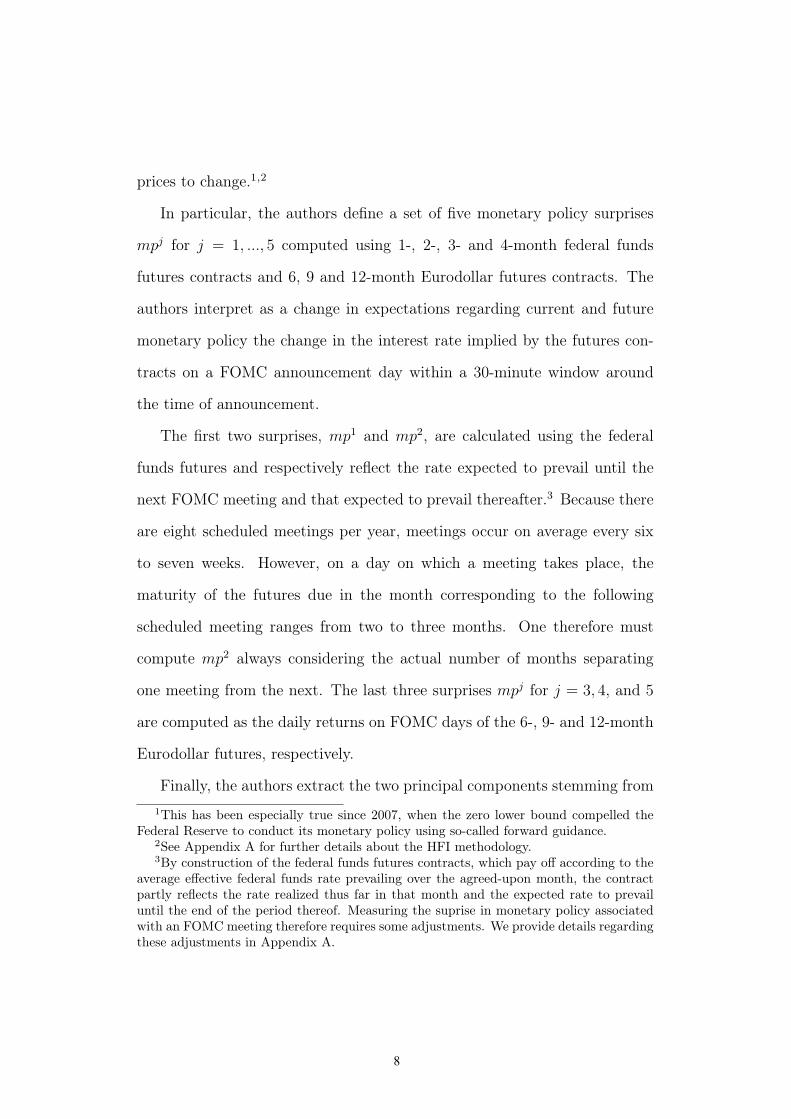
In particular, the authors define a set of five monetary policy surprises

mpj for j = 1, ..., 5 computed using 1-, 2-, 3- and 4-month federal funds

futures contracts and 6, 9 and 12-month Eurodollar futures contracts. The

authors interpret as a change in expectations regarding current and future

monetary policy the change in the interest rate implied by the futures con-

tracts on a FOMC announcement day within a 30-minute window around

the time of announcement.

The first two surprises, mp1 and mp2, are calculated using the federal

funds futures and respectively reflect the rate expected to prevail until the

next FOMC meeting and that expected to prevail thereafter.3 Because there

are eight scheduled meetings per year, meetings occur on average every six

to seven weeks. However, on a day on which a meeting takes place, the

maturity of the futures due in the month corresponding to the following

scheduled meeting ranges from two to three months. One therefore must

compute mp2 always considering the actual number of months separating

one meeting from the next. The last three surprises mpj for j = 3, 4, and 5

are computed as the daily returns on FOMC days of the 6-, 9- and 12-month

Eurodollar futures, respectively.

Finally, the authors extract the two principal components stemming from1This has been especially true since 2007, when the zero lower bound compelled the

Federal Reserve to conduct its monetary policy using so-called forward guidance.2See Appendix A for further details about the HFI methodology.3By construction of the federal funds futures contracts, which pay off according to the

average effective federal funds rate prevailing over the agreed-upon month, the contractpartly reflects the rate realized thus far in that month and the expected rate to prevailuntil the end of the period thereof. Measuring the suprise in monetary policy associatedwith an FOMC meeting therefore requires some adjustments. We provide details regardingthese adjustments in Appendix A.

8

8 9

Figure 2: Cumulated Series of Monetary Policy Shocks and Federal FundsRate

0

.02

.04

.06

.08

Fed

Fund

s R

ate

(%)

-.3

-.2

-.1

0

.1

.2

Targ

et F

acto

r

1990 1994 1998 2002 2006 2010 2014 2018

Target Factor Fed Funds Rate (rhs)

Notes: The figure plots the federal funds rate (dashed line, centeredaround zero) and the cumulated series of shocks to expectations aboutmonetary policy around the time of FOMC announcement days identi-fied as the target factor (solid line). The latter is the instrument we usefor the 1-year rate in the monthly SVAR.

this set of five monetary policy surprises, rotate them to give them a struc-

tural interpretation and label them the target factor and path factor. In

this paper, however, because we are interested in the effects of unexpected

changes in the stance of current monetary policy on Treasury liquidity pre-

mia, we focus on the target factor. This choice is also motivated by Jarociński

and Karadi (2020), who show in their online appendix that the target factor

performs marginally better as an instrument for the zero lower bound period.

The last step before estimating our monthly SVAR requires that we ag-

gregate the daily series of monetary policy surprises into a monthly series of

9

10

shocks that will ultimately serve our specification as an instrument. As in

Jarociński and Karadi (2020), we use the sum of the daily surprises occurring

in each month.

Figure 2 plots the series stemming from this aggregation of the target

factor (solid red line) on the left scale together with the federal funds rate (red

dashed line) on the right scale. By construction, the factor series cumulates

monetary policy surprises that relate to the target of the central bank, which

explains why the effective funds rate appears to be driven by the monetary

policy surprises. Recall that these surprises were identified to ensure that

they were exogenously driven by changes in the expectations about the future

target rate.

3.2 SVAR With External Instrument

Let us consider the following p-th order structural vector autoregressive

(SVAR) model with k endogenous variables:

AYt =

p∑s=1

ψsYt−s + εt, (1)

where Yt is a (k×1) vector of endogenous variables, A and the ψss are (k×k)

matrices of coefficients, and εt is a (k × 1) vector of structural innovations

such that E[εtε′t] = Ik and E[εtε

′s] = 0k for all t �= s.

We estimate the following reduced-form of (1):

Yt =

p∑s=1

φsYt−s + ut, (2)

where φs = A−1ψs, and ut is a (k × 1) vector of reduced form disturbances

10

10 11

shocks that will ultimately serve our specification as an instrument. As in

Jarociński and Karadi (2020), we use the sum of the daily surprises occurring

in each month.

Figure 2 plots the series stemming from this aggregation of the target

factor (solid red line) on the left scale together with the federal funds rate (red

dashed line) on the right scale. By construction, the factor series cumulates

monetary policy surprises that relate to the target of the central bank, which

explains why the effective funds rate appears to be driven by the monetary

policy surprises. Recall that these surprises were identified to ensure that

they were exogenously driven by changes in the expectations about the future

target rate.

3.2 SVAR With External Instrument

Let us consider the following p-th order structural vector autoregressive

(SVAR) model with k endogenous variables:

AYt =

p∑s=1

ψsYt−s + εt, (1)

where Yt is a (k×1) vector of endogenous variables, A and the ψss are (k×k)

matrices of coefficients, and εt is a (k × 1) vector of structural innovations

such that E[εtε′t] = Ik and E[εtε

′s] = 0k for all t �= s.

We estimate the following reduced-form of (1):

Yt =

p∑s=1

φsYt−s + ut, (2)

where φs = A−1ψs, and ut is a (k × 1) vector of reduced form disturbances

10

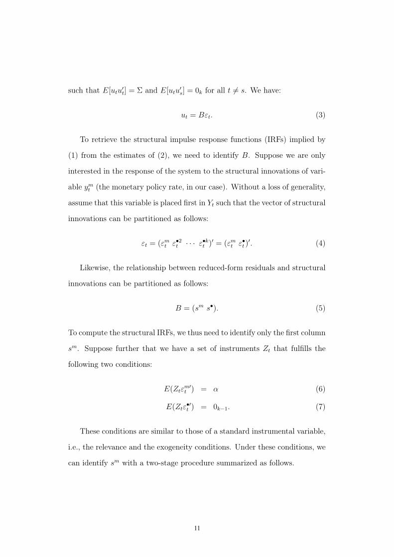
such that E[utu′t] = Σ and E[utu

′s] = 0k for all t �= s. We have:

ut = Bεt. (3)

To retrieve the structural impulse response functions (IRFs) implied by

(1) from the estimates of (2), we need to identify B. Suppose we are only

interested in the response of the system to the structural innovations of vari-

able ymt (the monetary policy rate, in our case). Without a loss of generality,

assume that this variable is placed first in Yt such that the vector of structural

innovations can be partitioned as follows:

εt = (εmt ε•2t · · · ε•kt )′ = (εmt ε•t )′. (4)

Likewise, the relationship between reduced-form residuals and structural

innovations can be partitioned as follows:

B = (sm s•). (5)

To compute the structural IRFs, we thus need to identify only the first column

sm. Suppose further that we have a set of instruments Zt that fulfills the

following two conditions:

E(Ztεm′t ) = α (6)

E(Ztε•′t ) = 0k−1. (7)

These conditions are similar to those of a standard instrumental variable,

i.e., the relevance and the exogeneity conditions. Under these conditions, we

can identify sm with a two-stage procedure summarized as follows.

11

12

I. First Stage: Estimate (2) and obtain the reduced-form residuals:

(umt u•

t ) = Yt −p∑

s=1

φsYt−s. (8)

Regress the reduced-form residuals that stem from the equation of the

variable of interest on the set of instruments:

umt = γZt + ξt, (9)

and obtain the fitted values umt = γZt.

II. Second Stage: Regress the reduced-form residuals u•t stemming from

the equations of the k−1 other variables y•t on the fitted values umt separately:

u•2t

u•3t

...

u•kt

=

umt 0 · · · 0

0 umt · · · 0

...... . . . ...

0 0 · · · umt

β•2

β•3

...

β•k

+

η•2t

η•3t...

η•kt

(10)

Column sm can finally be established using the following:

κ−1sm = (1 β•2 · · · β•k)′, (11)

where κ is a scaling factor identified up to a sign convention whose closed

solution can be found in Gertler and Karadi (2015, footnote 4).

System (1) can be finally estimated using the p reduced-form φss, the

((k − 1)× 1) vector β• and κ, by imposing the corresponding constraints on

the first column of B.

Notwithstanding, we are ultimately interested in computing the IRFs

12

12 13

resulting from VAR(p). Using lag operator L defined such that Lpηt = ηt−p,

Equation (2) is equivalent to the following:

(Ik − Lφ1 − · · · − Lpφp)Yt = ut. (12)

With Φ(L) = (Ik − Lφ1 − · · · − Lpφp), and provided that the VAR in (2) is

stable, we can obtain its infinite-order vector moving average representation

as follows:

Yt = Φ(L)−1ut−i =∞∑i=0

Γiut−i, (13)

where Γ0 = Ik and Γi =∑i

s=1 Γi−sφs for i = 1, 2, . . . . The notation included

in (13) is convenient, as it enables us to see that matrices Γi = ∂Yt+i/∂u′t are

the IRFs. Indeed, the j, k entry of Γi is the response of the j-th element of

Yt after i periods to a one-time unit shock to the k-th element of ut. Because

we identify the first column of B in the previous section, we can obtain a

causal interpretation of the effect of the orthogonalized shock of interest on

the whole system from ∂Yt+i/∂smεmt .

Finally, to account for potential conditional heteroskedasticity and avoid

any generated regressor problem, we use a recursive-design wild bootstrap

procedure to compute confidence intervals (CIs) for the IRFs.

The idea is to draw T independent observations {νt}t=1,...,T of a random

variable νt such that

νt =

+1 with probability 1/2

−1 with probability 1/2

(14)

13

14

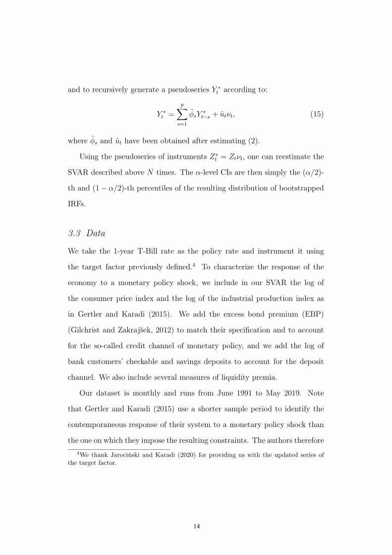
and to recursively generate a pseudoseries Y ∗t according to:

Y ∗t =

p∑s=1

φsY∗t−s + utνt, (15)

where φs and ut have been obtained after estimating (2).

Using the pseudoseries of instruments Z∗t = Ztνt, one can reestimate the

SVAR described above N times. The α-level CIs are then simply the (α/2)-

th and (1− α/2)-th percentiles of the resulting distribution of bootstrapped

IRFs.

3.3 Data

We take the 1-year T-Bill rate as the policy rate and instrument it using

the target factor previously defined.4 To characterize the response of the

economy to a monetary policy shock, we include in our SVAR the log of

the consumer price index and the log of the industrial production index as

in Gertler and Karadi (2015). We add the excess bond premium (EBP)

(Gilchrist and Zakrajšek, 2012) to match their specification and to account

for the so-called credit channel of monetary policy, and we add the log of

bank customers’ checkable and savings deposits to account for the deposit

channel. We also include several measures of liquidity premia.

Our dataset is monthly and runs from June 1991 to May 2019. Note

that Gertler and Karadi (2015) use a shorter sample period to identify the

contemporaneous response of their system to a monetary policy shock than

the one on which they impose the resulting constraints. The authors therefore4We thank Jarociński and Karadi (2020) for providing us with the updated series of

the target factor.

14

14 15

assume that the instrumental subsample is a representative characterization

of the way in which surprises in monetary policy affect the economy. We do

not need to make this assumption because Refcorp bonds were first issued in

1991.

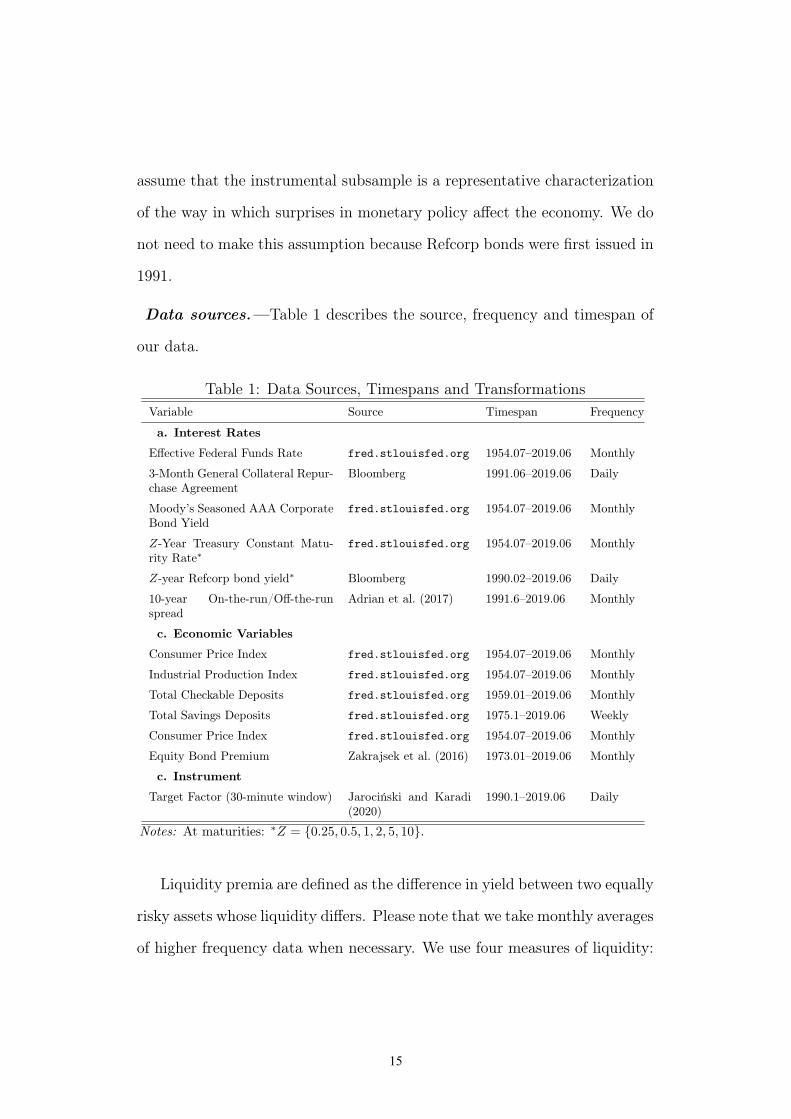
Data sources.—Table 1 describes the source, frequency and timespan of

our data.

Table 1: Data Sources, Timespans and TransformationsVariable Source Timespan Frequency

a. Interest Rates

Effective Federal Funds Rate fred.stlouisfed.org 1954.07–2019.06 Monthly

3-Month General Collateral Repur-chase Agreement

Bloomberg 1991.06–2019.06 Daily

Moody’s Seasoned AAA CorporateBond Yield

fred.stlouisfed.org 1954.07–2019.06 Monthly

Z-Year Treasury Constant Matu-rity Rate∗

fred.stlouisfed.org 1954.07–2019.06 Monthly

Z-year Refcorp bond yield∗ Bloomberg 1990.02–2019.06 Daily

10-year On-the-run/Off-the-runspread

Adrian et al. (2017) 1991.6–2019.06 Monthly

c. Economic Variables

Consumer Price Index fred.stlouisfed.org 1954.07–2019.06 Monthly

Industrial Production Index fred.stlouisfed.org 1954.07–2019.06 Monthly

Total Checkable Deposits fred.stlouisfed.org 1959.01–2019.06 Monthly

Total Savings Deposits fred.stlouisfed.org 1975.1–2019.06 Weekly

Consumer Price Index fred.stlouisfed.org 1954.07–2019.06 Monthly

Equity Bond Premium Zakrajsek et al. (2016) 1973.01–2019.06 Monthly

c. Instrument

Target Factor (30-minute window) Jarociński and Karadi(2020)

1990.1–2019.06 Daily

Notes: At maturities: ∗Z = {0.25, 0.5, 1, 2, 5, 10}.

Liquidity premia are defined as the difference in yield between two equally

risky assets whose liquidity differs. Please note that we take monthly averages

of higher frequency data when necessary. We use four measures of liquidity:

15

16

1. Our main measures of liquidity are the spreads between Resolution

Funding Corporation (Refcorp) bond yields and Treasury zero-coupon

bond yields. As argued by Longstaff (2002), Refcorp bonds are unique

because their principal is fully collateralized by Treasury bonds. Thus,

Refcorp bonds carry the same credit risk as Treasury bonds. Since

Treasury bonds are more liquid, comparing their prices to those of

Refcorp bonds serves as an ideal way of capturing liquidity premia.

2. Following Krishnamurthy and Vissing-Jorgensen (2012), we make use of

the difference between Moody’s Seasoned AAA Corporate Bond Yield

(mnemonic AAA) and the 10-Year Treasury Constant Maturity Rate

(GS10), which are both available on the Federal Reserve Bank of St.

Louis’ FRED database.

3. Alternatively, as suggested by Nagel (2016), we make use of the spread

between the 3-Month General Collateral Repurchase Agreement (GC

repo) Rate and the 3-Month Treasury Constant Maturity Rate. The

former is taken from Bloomberg (mnemonic USRGCGC ICUS Curncy)

and is computed as the midpoint between the bid and ask rates, and

the latter is obtained from FRED (GS3M).

4. Another measure of the liquidity premium is the spread between on-

the-run and off-the-run Treasury securities. The securities we use have

a 10-year maturity. See Adrian et al. (2017) for additional details.

Economic variables entering the VAR are monthly and come from the Fed-

eral Reserve Bank of St. Louis’ FRED database. These include the 1-year

16

16 17

Treasury yield (mnemonic GS1), the Consumer Price Index (CPIAUCSL), the

Industrial Production Index (INDPRO), the total checkable deposits (TCDSL),

and the total savings deposits (SAVINGSL). The equity bond premium is de-

rived from Zakrajsek et al. (2016).

The updated series of the first principal component of monetary policy

surprises for a 30-minute window around the time of FOMC announcements

was kindly provided to us by Jarociński and Karadi (2020) based on an

updated dataset of that used in Gürkaynak et al. (2005).

3.4 Results

Figure 3 plots the estimated structural IRFs (black solid lines) together with

the respective 95 percent bootstrapped CIs (black dashed lines). Each sub-

plot therefore shows the response of the abovementionned variable to a one-

standard deviation monetary policy shock (i.e., a monetary policy tighten-

ing). The red dotted lines show the IRFs stemming from the well-known

recursive identification, which places economic variables first (log CPI, log

IP, log deposits), and financial variables second (1-year rate, the EBP, and

liquidity premia). We included the latter to assess the robustness and the

advantage of the identification through external instruments.

A review of the IRFs obtained through the instrumental approach reveals

that a one-standard deviation positive shock to the target factor generates a

response of the 1-year rate of approximately 20 basis points that disapears

within two years.5 This monetary tightening triggers a response from the5Recall that the target factor is rescaled so as to match units with the first monetary

policy surprise, mp1t .

17

18

Figure 3: IRFs to Monetary Policy Shocks

-.20

.2

0 10 20 30 40 50

External Instrument

Cholesky

1-year rate

-.4-.2

0

0 10 20 30 40 50

CPI

-1-.5

0

0 10 20 30 40 50

IP

-1-.5

0

0 10 20 30 40 50

Deposits

-.10

.1

0 10 20 30 40 50

EBP

-.02

0.0

2

0 10 20 30 40 50

3-month spread

-.02

0.0

2

0 10 20 30 40 50

6-month spread

-.02

0.0

2

0 10 20 30 40 50

2-year spread

-.02

0.0

2

0 10 20 30 40 50

5-year spread

0.0

1.0

2

0 10 20 30 40 50

10-year spread

Impulse: 1-year rate. Instrument: Target Factor. First Stage: F = 17.61, R2 = 5.04, N = 334.CIs: Recursive wild bootstrap with 1000 replications, 0.95 level. Set Up: 2 lags, 1991.6 - 2019.5.Cholesky Order: 1y rate, CPI, IP, Deposits, EBP, 3m spread, 6m spread, 2y spread, 5y spread, 10y spread.

Notes: Each subgraph plots the IRF of the variable mentioned above to a one standarddeviation surprise monetary policy tightening (solid black line) together with the CIssurrounding it (dashed black lines) and the Cholesky-identified IRF (red dashed line). Seebelow the figure for more details.

economy consistent with theory: i) a significant and delayed decline in the

CPI level (approximately 20 bp) and ii) a significant decrease in output

(proxied by industrial production) within a year following the shock peaking

after around two years (approximately 50 bp.).

Regarding log deposits, the excess bond premium and liquidity premia,

the SVAR estimation corroborates the mechanisms behind both the deposit

and credit channels of monetary policy. First, the significant increase in the

EBP (approximately 50 bp), echoing Gertler and Karadi (2015), provides ev-

idence that monetary policy tightening deteriorates general credit conditions

18

18 19

for up to one year following the shock. Second, the significant long-lasting

decrease in log deposits (approximately 70 bp) coupled with the significant

increase in the liquidity premium at all maturities supports the mechanism

theorized in Drechsler et al. (2018).

When the monetary policy interest rate increases, rates paid on banks’

customer deposits do not adjust proportionally, leading to a decrease in ag-

gregate banks’ customer deposits: thus, the liquidity value of Treasuries

increases. Most importantly, the response of the liquidity premia across ma-

turities is characterized by a decreasing but significant relationship. Indeed,

the longer the maturity is, the less the premium increases, as longer-term

Treasuries are less liquid and are discounted more heavily when interest rates

rise. The responses of the liquidity premia are significant 1 to 2 years after

the policy shock. The response of the short-term (3-month) spread is approx-

imately one-tenth of the policy shock, whereas the response of the long-term

(10-year) spread is approximately one-fifth of the shock.

We obtain a similar overall result when we consider the Cholesky-identified

IRFs. It is worth noting that the shock under study is no longer identified us-

ing the instrument, as we rely on the ad hoc assumptions that a one-standard

deviation positive shock to the federal funds rate triggers a contemporane-

ous response of the financial variables included in the SVAR (the EBP and

the premia) but that it only affects the economy (the CPI and industrial

production) with a lag.

One noticeable strength of the instrumental approach is that it eradicates

the well-documented price puzzle. Furthermore, it produces a significant

response for all the spreads (which would likely be nonsignificant otherwise).

19

20

3.5 Robustness

Excluding the 2008 financial crisis.—As in Gertler and Karadi (2015),

we estimate the same model as in section 3.4 while excluding the 2008 finan-

cial crisis. In particular, we exclude the period between 2008.7 and 2009.6.

The results are quantitatively similar but somewhat less significant due to

the loss of observations (12 months plus lags).

Nonetheless, the chore implications of our benchmark specification pro-

vided in section 3.4 remain valid and the IRFs are significant at the 90 percent

level.

Using other measures of the liquidity premium.—Additionally, we

estimate the same model as in section 3.4 using different measures of liquidity

premia.

First, as a measure of short-term liquidity, we make use of the spread

between the 3-Month General Collateral Repurchase Agreement (GC repo)

Rate and the 3-Month Treasury Constant Maturity Rate as suggested by

Nagel (2016). For the measure of liquidity for longer maturities, we follow

Krishnamurthy and Vissing-Jorgensen (2012) and use the difference between

Moody’s Seasoned AAA Corporate Bond Yield and the 10-Year Treasury

Constant Maturity Rate.

The results of this alternative specification are shown in Figure 4. The

responses of the IP, the CPI, deposits and the EBP remain significant and

robust. The GC repo spread increases significantly (approximately 2 bp)

on impact, while the AAA spread significantly decreases (approximately 2

bp). Hence, this approach leads to a similar pattern according to which

20

20 21

long-maturity liquidity premia react less to monetary policy shocks.

Figure 4: IRFs to Monetary Policy Shocks, GC Repo Spread and AAA Spread

-.20

.2

0 10 20 30 40 50

External Instrument

Cholesky

1-year rate

-.2-.1

0.1

0 10 20 30 40 50

CPI

-1-.5

0

0 10 20 30 40 50

IP

-1-.5

0.5

0 10 20 30 40 50

Deposits

-.10

.1

0 10 20 30 40 50

EBP

-.02

0.0

2.0

4

0 10 20 30 40 50

GC repo spread-.0

50

.05

0 10 20 30 40 50

AAA spread

Impulse: 1-year rate. Instrument: Target Factor. First Stage: F = 11.81, R2 = 3.3, N = 348.CIs: Recursive wild bootstrap with 400 replications, 0.95 level. Set Up: 4 lags, 1990.2 - 2019.5.Cholesky Order: 1y rate, CPI, IP, Deposits, EBP, GC repo spread, AAA spread.

Notes: Each subgraph plots the IRF of the variable mentioned above to a one standarddeviation surprise monetary policy tightening (solid black line) together with the CIssurrounding it (dashed black lines) and the Cholesky-identified IRF (red dashed line). Seebelow the figure for more details.

Another common measure of the liquidity premium is the spread between

on-the-run and off-the-run Treasury securities (see Adrian et al. (2017) for

more details). The securities we use have a 10-year maturity, so we include

them in the SVAR instead of the AAA spread.

Figure 5 shows the results of this specification. While the GC repo spread

significantly increases on impact (approximately 2 bp), the on/off spread

somewhat decreases but remains insignificant following the monetary pol-

icy shock, which reinforces the view that longer-term liquidity premia react

21

22

relatively less to monetary policy.

Figure 5: IRFs to Monetary Policy Shocks, GC Repo Spread and On/OffSpread

-.10

.1.2

0 10 20 30 40 50

External Instrument

Cholesky

1-year rate

-.2-.1

0.1

0 10 20 30 40 50

CPI

-1-.5

0

0 10 20 30 40 50

IP

-1-.5

0.5

0 10 20 30 40 50

Deposits

0.1

.2

0 10 20 30 40 50

EBP

-.02

0.0

2.0

4

0 10 20 30 40 50

GC repo spread-.0

10

.01

0 10 20 30 40 50

On/Off spread

Impulse: 1-year rate. Instrument: Target Factor. First Stage: F = 12, R2 = 3.5, N = 334.CIs: Recursive wild bootstrap with 400 replications, 0.95 level. Set Up: 3 lags, 1991.6 - 2019.5.Cholesky Order: 1y rate, CPI, IP, Deposits, EBP, GC repo spread, On/Off spread.

Notes: Each subgraph plots the IRF of the variable mentioned above to a one standarddeviation surprise monetary policy tightening (solid black line) together with the CIssurrounding it (dashed black lines) and the Cholesky-identified IRF (red dashed line). Seebelow the figure for more details.

4 Conclusion

We have estimated the macrodynamic effects of monetary policy on the yield

curve through changes in liquidity premia. When the Fed raises interest rates,

the spread between less-liquid assets and Treasuries of the same maturity and

risk increases, which is significant 1 to 2 years after the policy shock. The

longer the maturity is, the lesser—but still significant—the increase in the

22

22 23

spread is.

Our empirical results point to the need to explicitly model the process of

obtaining deposits from liquid assets such as Treasuries to account for the

different liquidity premia at different maturities. Moreover, our results should

lead to a better understanding of the expectation hypothesis, which accounts

for the fact that monetary policy affects the term structure through liquidity

premia, and of real equilibrium interest rates and exchange rate fluctuations,

which are substantially influenced by liquidity premia fluctuations according

to recent research.

References

Adrian, T., Fleming, M., Shachar, O., and Vogt, E. (2017). Market liquidity

after the financial crisis. Annual Review of Financial Economics, 9:43–83.

Bok, B., Del Negro, M., Giannone, D., Giannoni, M., and Tambalotti, A.

(2018). A time-series perspective on safety, liquidity, and low interest

rates. Technical report, Federal Reserve Bank of New York.

Drechsler, I., Savov, A., and Schnabl, P. (2018). Liquidity, risk premia, and

the financial transmission of monetary policy. Annual Review of Financial

Economics, 10:309–328.

Engel, C. and Wu, S. P. Y. (2018). Liquidity and exchange rates: An empiri-

cal investigation. Technical report, National Bureau of Economic Research.

Faust, J., Swanson, E. T., and Wright, J. H. (2004). Identifying vars based on

23

24

high frequency futures data. Journal of Monetary Economics, 51(6):1107–

1131.

Ferreira, T. and Shousha, S. (2020). Scarcity of safe assets and global neutral

interest rates. FRB International Finance Discussion Paper, (1293).

Gertler, M. and Karadi, P. (2015). Monetary policy surprises, credit costs,

and economic activity. American Economic Journal: Macroeconomics,

7(1):44–76.

Gilchrist, S. and Zakrajšek, E. (2012). Credit spreads and business cycle

fluctuations. American Economic Review, 102(4):1692–1720.

Gonçalves, S. and Kilian, L. (2004). Bootstrapping autoregressions with

conditional heteroskedasticity of unknown form. Journal of Econometrics,

123(1):89–120.

Gürkaynak, R., Sack, B., and Swanson, E. (2005). Do actions speak louder

than words? The response of asset prices to monetary policy actions and

statements. International Journal of Central Banking, 1(1):55–93.

Jarociński, M. and Karadi, P. (2020). Deconstructing monetary policy

surprises—the role of information shocks. American Economic Journal:

Macroeconomics, 12(2):1–43.

Krishnamurthy, A. and Vissing-Jorgensen, A. (2012). The aggregate demand

for treasury debt. Journal of Political Economy, 120(2):233–267.

Kuttner, K. N. (2001). Monetary policy surprises and interest rates: Evi-

24

dence from the fed funds futures market. Journal of monetary economics,

47(3):523–544.

Longstaff, F. A. (2002). The flight-to-liquidity premium in US treasury bond

prices. Technical report, National Bureau of Economic Research.

Mertens, K. and Ravn, M. O. (2013). The dynamic effects of personal and

corporate income tax changes in the United States. American economic

review, 103(4):1212–47.

Nagel, S. (2016). The liquidity premium of near-money assets. The Quarterly

Journal of Economics, 131(4):1927–1971.

Nelson, E. (2003). The future of monetary aggregates in monetary policy

analysis. Journal of Monetary Economics, 50(5):1029–1059.

Reynard, S. and Schabert, A. (2010). Modeling monetary policy. SNB Work-

ing Paper 2010-4.

Stock, J. H. and Watson, M. W. (2012). Disentangling the channels of the

2007-2009 recession. Technical report, National Bureau of Economic Re-

search.

Zakrajsek, E., Lewis, K. F., and Favara, G. (2016). Updating the recession

risk and the excess bond premium. FEDS Notes, (2016-10):06.

25

24 25

dence from the fed funds futures market. Journal of monetary economics,

47(3):523–544.

Longstaff, F. A. (2002). The flight-to-liquidity premium in US treasury bond

prices. Technical report, National Bureau of Economic Research.

Mertens, K. and Ravn, M. O. (2013). The dynamic effects of personal and

corporate income tax changes in the United States. American economic

review, 103(4):1212–47.

Nagel, S. (2016). The liquidity premium of near-money assets. The Quarterly

Journal of Economics, 131(4):1927–1971.

Nelson, E. (2003). The future of monetary aggregates in monetary policy

analysis. Journal of Monetary Economics, 50(5):1029–1059.

Reynard, S. and Schabert, A. (2010). Modeling monetary policy. SNB Work-

ing Paper 2010-4.

Stock, J. H. and Watson, M. W. (2012). Disentangling the channels of the

2007-2009 recession. Technical report, National Bureau of Economic Re-

search.

Zakrajsek, E., Lewis, K. F., and Favara, G. (2016). Updating the recession

risk and the excess bond premium. FEDS Notes, (2016-10):06.

25

26

A Methodology

In this appendix, we provide additional details regarding the methodology.

We expose how one can formally extract changes in expectations about future

monetary policy using futures data and how one can rotate the resulting fac-

tors into interpretable dimensions of the Fed’s conduct through its monetary

policy.

Identifying Expectations Shocks.—Let us denote by ff 1t−∆t as the set-

tlement rate implied by the federal funds rate futures contract expiring within

the month, ∆t days before a scheduled FOMC announcement. By construc-

tion of the futures contracts, which pay off according to the average effective

federal funds rate prevailing over the agreed-upon month, ff1t−∆t partly re-

flects the rate realized thus far in the given month, r0, and the expected rate

to prevail until the end of the period thereof, r1. Accordingly, by denoting

d1 as the day of the month on which an FOMC meeting will take place and

D1 as the number of days in that same month, we have the following:

ff 1t−∆t =

d1

D1r0 +

D1 − d1

D1Et−∆t[r1] + ρ1t−∆t, (16)

where ρ1 accounts for any (risk, term or liquidity) premium present in the

contract. Assuming that there is no systematic change in premium ρ1 within

an FOMC announcement day, the surprise associated with a change in the

federal funds target rate, Et[r1]− Et−1[r1], is

mp1t =D1

D1 − d1(ff 1

t − ff 1t−1). (17)

Similarly, one can measure the change in expectation, mp2t , regarding

26

26 27

the rate that will prevail after the next FOMC meeting, r2, by examining

the futures of corresponding maturity. Because there are eight scheduled

meetings per year, the next meeting arises within the next two months.6 By

denoting m as the number of months separating the current meeting from

the next, it follows that:

ff 1+mt−∆t =

d1+m

D1+mEt−∆t[r1] +

D1+m − d1+m

D1+mEt−∆t[r2] + ρ1+m

t−∆t, (18)

where the superscript i in ff it−∆t indicates the number of months from t−∆t

within which the futures due date occurs. The change in expectation is

therefore characterized by:

mp2t =D1+m

D1+m − d1+m

[(ff 1+m

t − ff 1+mt−1 )− d1+m

D1+mmp1t

]. (19)

There are two particular cases one needs to account for. First, when a

meeting happens late in a month, the weight given to the surprise is relatively

high. To prevent from the potential noise in the data from affecting our

measurement, when a meeting occurs within the last seven days of a month,

we take the unweighted change in the next month’s futures price as the

monetary policy surprise. Second, for meetings taking place on the first day

of a month, we make use of the unweighted price difference between the

federal funds futures rate due in the month of the meeting and that due in

the previous month.

Finally, for the remaining contracts, namely, the 6-, 9- and 12-month

Eurodollar futures (with a price denoted by edit), one can directly take the6NOte that Gürkaynak et al. (2005) assume unscheduled meetings to be expected as

happening with zero probability.

27

28

daily return as the surprise itself due to their spot settlement nature. Thus,

for j = 4, 5, 6 and i = 6, 9, 12 respectively, we have

mpj = edit − edit−1. (20)

Extracting the target and the path factor.—Let X be a (T×n) matrix

whose entries correspond to the above-defined monetary policy surprises mpjt

for j = 1, ..., n and t = 1, ..., T , that is, the surprise component of the daily

change in federal funds futures and Eurodollar futures rates solely associated

with FOMC announcements.7

Let us assume X to be generated by the following factor model:

X = FΛ + ν, (21)

where F is a (T×�) matrix of (� < n) unobserved factors, Λ is a (�×n) matrix

of factor loadings, and ν is a matrix of orthogonal disturbances. Gürkaynak

et al. (2005) show that the response of futures prices is sufficiently character-

ized by two factors (i.e., � = 2). We therefore estimate F = {F1t, F2t}t=1,...,T

through principal-component analysis.

Because the two factors yielded by this method are chosen to maximize

the share of explained variance, they lack structural interpretation. Gürkay-

nak et al. (2005) rotate F1 and F2 to obtain Z1 and Z2. Namely, we define:

Z = FU, (22)

such that U is a (2 × 2) orthogonal matrix with Z2 being associated, on7We normalize the columns of X so that they have zero mean and unit variance.

28

28 29

average, with no change in the federal funds futures rate for the current

month. To recover an interpretation as to the magnitude of these factors, we

rescale Z1 (Z2) to match its units with mp1 (mp4).

According to Gürkaynak et al. (2005), this rotation allows us to see Z1

and Z2 as the target factor and the path factor, respectively. This is the

case because Z1 is defined such as to drive surprises in the current target

rate on FOMC announcement days, while Z2 reflects everything (unrelated

to the federal funds target rate) that causes changes to expectations of future

monetary policy. Next, we describe the way in which the target factor serves

as an external instrument for the estimation of our structural VAR.

Rotation of the Factors.—Gürkaynak et al. (2005) rotate F1 and F2 to

obtain Z1 and Z2. Namely, they define

Z = FU, (23)

where

U =

u11 u12

u21 u22

′

, (24)

such that U is a (2 × 2) orthogonal matrix, with Z2 being associated, on

average, with no change in the federal funds futures rate for the current

month. The orthogonality between Z1 and Z2 requires that:

E(Z1Z2) = u11u12 + u21u22 = 0. (25)

29

30

Then, because:

F1 =u22Z1 − u12Z2

u11u22 − u12u21

, (26)

F2 =u21Z1 − u11Z2

u12u21 − u11u22

, (27)

one can assume that Z2 has no impact on mp1 by imposing the final restric-

tion:

λ2u11 − λ1u12 = 0, (28)

where λ1 and λ2 are the loadings on mp1 of F1 and F2, respectively. To recover

an interpretation as to the magnitude of these factors, one can rescale Z1 (Z2)

to match its units with mp1 (mp4). Rotation matrix U is obtained by solving

the last four equations.

In the words of Gürkaynak et al. (2005), this rotation allows us to see

Z1 and Z2 as the target factor and the path factor, respectively. This is the

case because Z1 is defined such as to drive surprises in the current target

rate on FOMC announcement days, while Z2 reflects everything (unrelated

to the federal funds target rate) that causes changes to expectations of future

monetary policy.

30

30

2021-14 Maxime Phillot, Samuel Reynard: Monetarypolicyfinancialtransmissionandtreasury liquidity premia

2021-13 Martin Indergand, Gabriela Hrasko: Does the market believe in loss-absorbing bank debt?

2021-12 Philipp F. M. Baumann, Enzo Rossi, Alexander Volkmann: Whatdrivesinflationandhow?Evidencefromadditivemixed models selected by cAIC

2021-11 Philippe Bacchetta, Rachel Cordonier, Ouarda Merrouche: The rise in foreign currency bonds: the role of US monetary policy and capital controls

2021-10 AndreasFuster,TanSchelling,PascalTowbin: Tiers of joy? Reserve tiering and bank behavior in anegative-rate environment

2021-09 AngelaAbbate,DominikThaler: Optimal monetary policy with the risk-taking channel

2021-08 ThomasNitschka,ShajivanSatkurunathan: Habits die hard: implications for bond and stockmarkets internationally

2021-07 LucasFuhrer,NilsHerger: Real interest rates and demographic developments across generations: A panel-data analysis over twocenturies

2021-06 WinfriedKoeniger,BenediktLennartz, Marc-Antoine Ramelet: On the transmission of monetary policy to thehousing market

2021-05 RomainBaeriswyl,LucasFuhrer,PetraGerlach-Kristen,Jörn Tenhofen: The dynamics of bank rates in a negative-rate environment – the Swiss case

2021-04 RobertOleschak: Financial inclusion, technology and their impacts onmonetaryandfiscalpolicy:theoryandevidence

2021-03 DavidChaum,ChristianGrothoff,ThomasMoser: How to issue a central bank digital currency

2021-02 JensH.E.Christensen,NikolaMirkov: The safety premium of safe assets

2021-01 TillEbner,ThomasNellen,JörnTenhofen: The rise of digital watchers

2020-25 LucasMarcFuhrer,Marc-AntoineRamelet, Jörn Tenhofen: Firms‘participationintheCOVID-19loanprogramme

2020-24 BasilGuggenheim,SébastienKraenzlin,Christoph Meyer: (In)Efficienciesofcurrentfinancialmarketinfrastructures–acallforDLT?

2020-23 MiriamKoomen,LaurenceWicht: Demographics, pension systems, and the currentaccount: an empirical assessment using the IMFcurrent account model

2020-22 YannicStucki,JacquelineThomet: AneoclassicalperspectiveonSwitzerland’s1990sstagnation

2020-21 FabianFink,LukasFrei,OliverGloede: Short-term determinants of bilateral exchange rates:A decomposition model for the Swiss franc

2020-20 LaurenceWicht: A multi-sector analysis of Switzerland’s gains from trade

2020-19 TerhiJokipii,RetoNyffeler,StéphaneRiederer: Exploring BIS credit-to-GDP gap critiques: the Swiss case

Recent SNB Working Papers