moleculardynamics simulationofwaterand …
TRANSCRIPT

MOLECULAR DYNAMICSSIMULATION OF WATER AND
AQUEOUS SOLUTIONS
Igor ShvabDissertation
submitted in ful�llment of requirements for the degree ofDoctor of Philosophy
Centre for Molecular SimulationFaculty of Information and Communication Technologies
Swinburne University of Technology
February 2014

Abstract
The objectives of this work is to use molecular dynamic simulation to systematically
investigate all basic properties of water and aqueous solutions of neon, argon, krypton,
xenon and methane in the liquid phase.
The structural properties of pure water at densities 1, 0.8, and 0.6 g/cm3, and aqueous
nonpolar solute mixtures at constant density 1g/cm3 have been investigated in the canon-
ical NVT ensemble over the temperature range 278 - 750 K. We have used and compared
several water models, namely the ab initio MCYna model and rigid SPC/E and SPC/Fw
models to study hydrogen-bond network and shell structure of bulk water. Structure of
aqueous solutions has been investigated with the help of combined MCYna + LJ and
SPC/E + LJ potentials. For aqueous solutions water-water interaction were obtained
from the MCYna and SPC/E water models, whereas water-solute and solute-solute in-
teractions were calculated with the help of the Lennard-Jones potential. Simulations
show that SPC/E, SPC/Fw, and to a lesser degree MCYna models underestimate wa-
ter structure and the level of hydrogen bonding in the high temperature region. The
presence of nonpolar solutes in small concentrations appears to have local strengthening
e�ect on water structure, while at higher concentrations solute particles clearly prevent
water molecules from forming hydrogen bonds.
Polarization properties of water and aqueous nonpolar solute mixtures have been thor-
oughly investigated using MCYna + LJ potential model. The dielectric constant and
dipole moment of pure water and aqueous solutions have been found. The dielectric
constant of bulk water given by ab initio polarizable MCYna model is in good agreement
with experimental data. Introduction of nonpolar solutes decreases polarization prop-
erties of water. The dielectric constant and average dipole moment of the mentioned
mixtures are decreasing with temperature and solute concentration.
A novel technique of statistical averages has been applied to study all thermodynamic
properties of water and water-methane mixtures in the liquid phase. Namely, thermal
pressure coe�cient, isothermal and adiabatic compressibilities, thermal expansion coef-
�cient, isochoric and isobaric heat capacities, Joule-Thompson coe�cient, and speed of
sound of water and water-methane mixtures. Results obtained by using nonpolarizable
SPC/E and TIP4P/2005 water models show qualitative agreement with experimental

ii
data at temperatures up to 400 K. Comparison of the present results with results ob-
tained from polarizable MCYna model indicate superiority of the polarizable potential
over nonpolarizable SPC/E and TIP4P/2005 potentials. In case of water-methane mix-
tures, simulated results show that methane decreases heat capacities and compressibili-
ties, and increases expansion coe�cient and speed of sound comparing to pure water.
Finally, transport properties of aqueous solutions of neon, argon, krypton, xenon and
methane have been also calculated in the liquid phase. The presence of nonpolar so-
lutes like methane or noble gases decreases di�usion coe�cient of water. This decrease
is mainly proportional to the solute concentration number. Comparison of di�usion co-
e�cients of noble gases and methane clearly indicate their mass and size dependency.
Nonpolar particles with large mass and atomic diameter di�use in water more slowly
than light particles. Velocity autocorrelation functions also indicate speci�c changes in
solvation shell structure caused by solute particles.

Acknowledgements
I would like to acknowledge and thank my supervisors Prof. Richard J. Sadus and Prof.
Billy D Todd for their positive direction and continuing support. In particular, I am
grateful to my principal supervisor Prof. Richard Sadus for his invaluable encouragement,
professionalism and patience to achieve quality. Both of my supervisors gifted me the
best attributes of a researcher through their scienti�c knowledge, professional attitude
and fantastic interpersonal skill.
I would like to thank Swinburne University of Technology for �nancial support through
a Swinburne University Postgraduate Research Award scholarship (SUPRA). This work
also received computational time from Victorian Partnership for Advanced Computing
(VPAC).
Thanks to other academic sta� and students in the Centre for Molecular Simulation and
SUCCESS department for all encouraging discussions and friendly atmosphere.
Finally, I would like to thank my family whose love continues to encourage me, as it has
always done.
iii

Declaration
I hereby declare that this thesis entitled "Molecular Dynamics Simulation of Water and
Aqueous Solutions" is my own work. To the best of my knowledge, it contains no
materials previously published by other persons except where reference is made in the
text of the thesis.
Igor Shvab
February 2014
iv

Publications
1. I. Shvab and R. J. Sadus. Structure and polarization properties of water: Molecular
dynamics with a nonadditive intermolecular potential. Physical Review E, 85,051509 (2012).
2. I. Shvab and R. J. Sadus. Dielectric and structural properties of aqueous nonpolar
solute mixtures. J. Chem. Phys, 137, 124501 (2012).
3. I. Shvab and R. J. Sadus. Intermolecular potentials and the accurate prediction of
the thermodynamic properties of water. J. Chem. Phys, 139, 194505 (2013).
4. I. Shvab and R. J. Sadus. Thermodynamic properties and di�usion of water +
methane binary mixtures. (Submitted to J. Chem. Phys.)
v

Contents
Abstract i
Acknowledgements iii
Declaration of Authorship iv
Publications v
Notations ix
Physical Constants xii
List of Tables xiii
List of Figures xiv
1 Introduction 11.1 Aims and Motivations . . . . . . . . . . . . . . . . . . . . . . . . . . . . . 11.2 Background and current progress . . . . . . . . . . . . . . . . . . . . . . . 3
1.2.1 Water structure . . . . . . . . . . . . . . . . . . . . . . . . . . . . . 31.2.2 Polarization properties . . . . . . . . . . . . . . . . . . . . . . . . . 51.2.3 Thermodynamic properties . . . . . . . . . . . . . . . . . . . . . . 61.2.4 Transports properties . . . . . . . . . . . . . . . . . . . . . . . . . 9
1.3 Outline of the thesis . . . . . . . . . . . . . . . . . . . . . . . . . . . . . . 10
2 Molecular Dynamic Simulation 122.1 Water-water interaction . . . . . . . . . . . . . . . . . . . . . . . . . . . . 14
2.1.1 Water molecule . . . . . . . . . . . . . . . . . . . . . . . . . . . . . 142.1.2 Water models, criteria . . . . . . . . . . . . . . . . . . . . . . . . . 192.1.3 Rigid water models . . . . . . . . . . . . . . . . . . . . . . . . . . . 21
2.1.3.1 SPC . . . . . . . . . . . . . . . . . . . . . . . . . . . . . . 212.1.3.2 TIP3P . . . . . . . . . . . . . . . . . . . . . . . . . . . . . 232.1.3.3 SPC/E . . . . . . . . . . . . . . . . . . . . . . . . . . . . 232.1.3.4 TIP4P/2005 . . . . . . . . . . . . . . . . . . . . . . . . . 24
vi

Table of Contents vii
2.1.3.5 MCY (Matsuoka-Clementi-Yoshimine) . . . . . . . . . . . 252.1.3.6 TIP5P . . . . . . . . . . . . . . . . . . . . . . . . . . . . . 272.1.3.7 NvdE . . . . . . . . . . . . . . . . . . . . . . . . . . . . . 28
2.1.4 Polarizable water models . . . . . . . . . . . . . . . . . . . . . . . . 282.1.4.1 SPC/FQ . . . . . . . . . . . . . . . . . . . . . . . . . . . 292.1.4.2 TIP4P/FQ . . . . . . . . . . . . . . . . . . . . . . . . . . 292.1.4.3 GCPM (Gaussian charge polarizable model) . . . . . . . 302.1.4.4 BKd3 (Baranyai-Kiss) . . . . . . . . . . . . . . . . . . . . 302.1.4.5 MCYna (Matsuoka-Clementi-Yoshimine nonadditive) . . . 30
2.1.5 Flexible water models . . . . . . . . . . . . . . . . . . . . . . . . . 322.1.5.1 SPC/Fw . . . . . . . . . . . . . . . . . . . . . . . . . . . 332.1.5.2 TIP4P/2005f . . . . . . . . . . . . . . . . . . . . . . . . . 342.1.5.3 MCYL (Matsuoka-Clementi-Yoshimine-Lie) . . . . . . . . 34
2.1.6 Ab initio water models . . . . . . . . . . . . . . . . . . . . . . . . . 342.1.7 Improving water models . . . . . . . . . . . . . . . . . . . . . . . . 39
2.2 Water-solute interaction . . . . . . . . . . . . . . . . . . . . . . . . . . . . 412.2.1 Methane clathrate . . . . . . . . . . . . . . . . . . . . . . . . . . . 422.2.2 Hydrophobic interaction . . . . . . . . . . . . . . . . . . . . . . . . 44
2.2.2.1 Water-Neon . . . . . . . . . . . . . . . . . . . . . . . . . . 472.2.2.2 Water-Argon . . . . . . . . . . . . . . . . . . . . . . . . . 472.2.2.3 Water-Krypton . . . . . . . . . . . . . . . . . . . . . . . . 482.2.2.4 Water-Xenon . . . . . . . . . . . . . . . . . . . . . . . . . 492.2.2.5 Water-Methane . . . . . . . . . . . . . . . . . . . . . . . . 49
2.3 Simulation details . . . . . . . . . . . . . . . . . . . . . . . . . . . . . . . . 532.3.1 Simulation ensemble . . . . . . . . . . . . . . . . . . . . . . . . . . 532.3.2 Equations of motion . . . . . . . . . . . . . . . . . . . . . . . . . . 532.3.3 Initial lattice con�guration . . . . . . . . . . . . . . . . . . . . . . 542.3.4 Initial random velocity . . . . . . . . . . . . . . . . . . . . . . . . . 542.3.5 Constant temperature . . . . . . . . . . . . . . . . . . . . . . . . . 552.3.6 Force calculation . . . . . . . . . . . . . . . . . . . . . . . . . . . . 552.3.7 Integration of motion . . . . . . . . . . . . . . . . . . . . . . . . . . 562.3.8 Constraint method . . . . . . . . . . . . . . . . . . . . . . . . . . . 572.3.9 Periodic boundaries . . . . . . . . . . . . . . . . . . . . . . . . . . 572.3.10 Treatment of long-range and Coulomb interactions . . . . . . . . . 59
3 Calculation of Thermodynamic Properties from Molecular Simulation 633.1 Thermodynamic quantities from �uctuation theory . . . . . . . . . . . . . 633.2 Thermodynamic quantities from statistical mechanics theory . . . . . . . . 65
3.2.1 Thermal pressure coe�cient . . . . . . . . . . . . . . . . . . . . . . 673.2.2 Compressibilities . . . . . . . . . . . . . . . . . . . . . . . . . . . . 673.2.3 Thermal expansion coe�cient . . . . . . . . . . . . . . . . . . . . . 683.2.4 Heat capacities . . . . . . . . . . . . . . . . . . . . . . . . . . . . . 693.2.5 Speed of sound . . . . . . . . . . . . . . . . . . . . . . . . . . . . . 703.2.6 Joule-Thomson coe�cient . . . . . . . . . . . . . . . . . . . . . . . 70
3.3 Calculation of thermodynamic quantities in the NVT ensemble . . . . . . 71
4 Molecular Structure and Hydrogen Bonding in Aqueous Solutions 74

Table of Contents viii
4.1 Simulation details . . . . . . . . . . . . . . . . . . . . . . . . . . . . . . . . 774.2 Molecular structure and hydrogen bonding in bulk water . . . . . . . . . . 78
4.2.1 Structural properties along the isochore at 1 g/cm3. . . . . . . . . 784.2.2 Structural properties along the isochore at 0.8 g/cm3. . . . . . . . 804.2.3 Structural properties along the isochore at 0.6 g/cm3. . . . . . . . 814.2.4 Shell structure . . . . . . . . . . . . . . . . . . . . . . . . . . . . . 83
4.3 Molecular structure and hydrogen bonding in aqueous nonpolar solutemixtures . . . . . . . . . . . . . . . . . . . . . . . . . . . . . . . . . . . . . 874.3.1 Water-solute radial distribution functions . . . . . . . . . . . . . . 874.3.2 Structure of the solvation shells . . . . . . . . . . . . . . . . . . . . 894.3.3 One-phase region . . . . . . . . . . . . . . . . . . . . . . . . . . . . 94
5 Polarization Properties of Aqueous Nonpolar Solute Mixtures 975.1 Current theories of dielectrics . . . . . . . . . . . . . . . . . . . . . . . . . 975.2 Polarization properties of bulk water . . . . . . . . . . . . . . . . . . . . . 101
5.2.1 Dielectric constant . . . . . . . . . . . . . . . . . . . . . . . . . . . 1025.2.2 Dipole moment . . . . . . . . . . . . . . . . . . . . . . . . . . . . . 105
5.3 Polarization properties of aqueous nonpolar solute mixtures . . . . . . . . 1065.3.1 Dielectric constant . . . . . . . . . . . . . . . . . . . . . . . . . . . 1075.3.2 Comparison of MD and analytical calculations of dielectric constants1105.3.3 Dipole moment . . . . . . . . . . . . . . . . . . . . . . . . . . . . . 112
6 Thermodynamic Properties of Water and Aqueous Nonpolar SoluteMixtures 1166.1 Thermodynamics of solvation . . . . . . . . . . . . . . . . . . . . . . . . . 1196.2 Reference data for water . . . . . . . . . . . . . . . . . . . . . . . . . . . . 1246.3 Pressure . . . . . . . . . . . . . . . . . . . . . . . . . . . . . . . . . . . . . 1246.4 Thermal pressure coe�cient . . . . . . . . . . . . . . . . . . . . . . . . . . 1276.5 Isothermal and adiabatic compressibilities . . . . . . . . . . . . . . . . . . 1296.6 Thermal expansion coe�cient . . . . . . . . . . . . . . . . . . . . . . . . . 1326.7 Isochoric and isobaric heat capacities . . . . . . . . . . . . . . . . . . . . . 1356.8 Speed of sound . . . . . . . . . . . . . . . . . . . . . . . . . . . . . . . . . 1406.9 Joule-Thomson coe�cient . . . . . . . . . . . . . . . . . . . . . . . . . . . 142
7 Transport Properties 1457.1 Di�usion theories . . . . . . . . . . . . . . . . . . . . . . . . . . . . . . . . 145
7.1.1 Trajectory analysis . . . . . . . . . . . . . . . . . . . . . . . . . . . 1507.1.2 Correlation function . . . . . . . . . . . . . . . . . . . . . . . . . . 151
7.2 Di�usion coe�cients of aqueous nonpolar solute mixtures . . . . . . . . . 1527.3 VACF and the shell structure . . . . . . . . . . . . . . . . . . . . . . . . . 159
8 Conclusions and Recommendations 162
Bibliography 168

Notations
AbbreviationsSPC simple point charge
SPC/E extended simple point charge
SPC/Fw �exible simple point charge
SPC/Fd �exible simple point charge
SPC/FQ simple point charge with �uctuating charges
TIP3P transferable intermolecular potential three point
TIP4P transferable intermolecular potential four point
TIP4P/FQ transferable intermolecular potential four point with �uctuating charges
TIP4P/2005 transferable intermolecular potential four point 2005
TIP5P transferable intermolecular potential �ve point
MCY Matsuoka-Clementi-Yoshimine water model
MCYL Matsuoka-Clementi-Yoshimine-Lie �exible water model
MCYna Matsuoka-Clementi-Yoshimine water model with nonadditive terms
BNS Ben-Naim and Stillinger model
ST2 Stillinger and Rahman model
PPC polarizable point charge model
GCPM Gaussian charge polarizable model
RPOL Revised polarizable model
LJ Lennard-Jones
CHARMM Chemistry at HARvard Macromolecular Mechanics
DL_POLY Daresbury Laboratory Polyatomic
MD molecular dynamics
MC Monte Carlo
AIMD Ab initio molecular dynamics
ix

Notations x
CPMD Car-Parrinello molecular dynamics
PIMD Path integral molecular dynamics
T temperature
Tc critical temperature
Tm melting temperature
TMD temperature of maximum density
RDF radial distribution function
EOS equation of state
Exp. experiment
Ref. reference
fcc face centered cubic
CGM conjugate gradient method
MPI message passing interface
PBC periodic boundary conditions
IAPWS international association for the properties of water and steam
∆t simulation step length
t total simulation time
ρ density
p pressure
P total linear momentum
m mass of a single atom/molecule
M total mass of the system
V volume
N number of molecules/atoms
U molar potential energy
K molar kinetic energy
E molar internal energy
Πmn derivatives of partition function with respect to temperature and volume
S Entropy
G Gibbs energy
A Helmholtz energy
H Enthalpy
∆S changes in Entropy upon solvation

Notations xi
∆G changes in Gibbs energy upon solvation
∆A changes in Helmholtz energy upon solvation
∆H changes in Enthalpy upon solvation
α electronic polarizability
εr dielectric constant
µ dipole moment
rij relative position of particles i and j
ri position of the particle i
uij potential energy between particles i and j
v velocity of the particle
a acceleration of the particle
fij force between particles i and j
L length of the side of simulation box
qi charge of atom i or on site i inside of the molecule
l1 oxygen-hydrogen bond length
l2 the distance between oxygen and the displaced charge (dummy) site
φ angle between the hydrogen-oxygen bond and the oxygen-dummy line
θ bond angle between two oxygen-hydrogen bonds
σ Lennard-Jones length constant
ε Lennard-Jones energy constant
Cv isochoric heat capacity
Cp isobaric heat capacity
∆Cv Cv di�erence between the Cv of pure water and mixture
∆Cp Cp di�erence between the Cp of pure water and mixture
γv thermal pressure coe�cient
κT isothermal compressibility
κS adiabatic compressibility
αp thermal expansion coe�cient
ω0 speed of sound at zero frequency
µJT Joule-Thomson coe�cient

Physical Constants
e elementary positive charge (1.602176565(35)×10−19 C)
k Boltzmann constant (1.380662 × 10⁻²³ J/K)
R universal gas constant (8.31441 J mol−1 K−1 )
Na Avogadro number (6.022045 × 10²³ mol−1 )
Å Ångström 10−10 m
nm nano meter (10−9 m)
ns nano second (10−9 s)
ps pico second (10−12 s)
fs femto second (10−15 s)
D Debye (unit of molecular dipole moment) (≈ 3.33564×10⁻³⁰ C m)
ε0 vacuum permittivity (≈ 8.854187817620×10⁻¹² C2 N−1m−2)
xii

List of Tables
2.1 Intermolecular parameters used in the MCY and MCYna intermolecularpotential. Values are in atomic units. . . . . . . . . . . . . . . . . . . . . . 27
2.2 Parameters for some water molecules. Angles θ, ϕ, distances l1, l2, andcharges q1, q2, and q3 are shown in Figure 2.5. . . . . . . . . . . . . . . . . 38
3.1 Summary of thermodynamic functions in terms of partial derivatives ofpartition function Π(β, V, N). . . . . . . . . . . . . . . . . . . . . . . . . . 72
4.1 Positions of the �rst minima of the MCYna RDFs together with noo valuesalong the 1, 0.8, and 0.6 g/cm3 isochores. . . . . . . . . . . . . . . . . . . 86
4.2 Lennard-Jones potential parameters used for water-solute and solute-solutepair interactions (Guillot and Guissani, 1993). . . . . . . . . . . . . . . . . 87
5.1 Dielectric constants for the MCYna and SPCE models along the 1, 0.8,and 0.6 g/cm3 isochores. . . . . . . . . . . . . . . . . . . . . . . . . . . . . 104
6.1 Comparison with experiment for the thermodynamic properties of severalwater models at 298K and 0.1 MPa. . . . . . . . . . . . . . . . . . . . . . 123
xiii

List of Figures
2.1 Simple representation of water molecule. . . . . . . . . . . . . . . . . . . . 152.2 Schematic representation of the water dimer. . . . . . . . . . . . . . . . . 162.3 Schematic representation of the tetrahedral shape of water. . . . . . . . . 172.4 Hydrogen bond network in water. . . . . . . . . . . . . . . . . . . . . . . . 182.5 Schematic representation of water models. . . . . . . . . . . . . . . . . . . 222.6 Structure of the MCYna water molecule. . . . . . . . . . . . . . . . . . . . 252.7 De�nition of the MCY water dimer geometry. . . . . . . . . . . . . . . . . 262.8 Methane clathrate. . . . . . . . . . . . . . . . . . . . . . . . . . . . . . . . 432.9 Formation of hydrophobic interaction. . . . . . . . . . . . . . . . . . . . . 452.10 Ne-H2O coordinate system. . . . . . . . . . . . . . . . . . . . . . . . . . . 472.11 Ar-H2O coordinate system. . . . . . . . . . . . . . . . . . . . . . . . . . . 482.12 CH4-H2O coordinate system. . . . . . . . . . . . . . . . . . . . . . . . . . 502.13 Periodic boundary conditions, minimum image convention and spherical
cuto� radius. . . . . . . . . . . . . . . . . . . . . . . . . . . . . . . . . . . 58
4.1 Radial distribution function calculation . . . . . . . . . . . . . . . . . . . . 754.2 Temperature dependence of the water RDFs along the 1 g/cm3 isochore. . 804.3 Temperature dependence of the water RDFs along the 0.8 g/cm3 isochore. 814.4 Temperature dependence of the water RDFs along the 0.6 g/cm3 isochore. 824.5 Oxygen-hydrogen coordination numbers at densities 1, 0.8, and 0.6 g/cm3 844.6 Solute-oxygen RDFs for water-solute systems at 298 K. . . . . . . . . . . . 894.7 Comparison of pure water and mixture RDFs. . . . . . . . . . . . . . . . . 904.8 Argon-oxygen, oxygen-oxygen, and oxygen-hydrogen coordination num-
bers at di�erent argon mole fractions. . . . . . . . . . . . . . . . . . . . . 914.9 Coordination numbers of di�erent aqueous solutions at 298 K as a function
of solute concentration. . . . . . . . . . . . . . . . . . . . . . . . . . . . . . 93
5.1 Dielectric constant εr of bulk water at densities 1, 0.8, and 0.6 g/cm3. . . 1035.2 Water dipole moments distribution. . . . . . . . . . . . . . . . . . . . . . . 1065.3 Water dipole moments at densities 1, 0.8, and 0.6 g/cm3. . . . . . . . . . 1075.4 Dielectric constants of water-neon, water-argon, and water-methane mix-
tures . . . . . . . . . . . . . . . . . . . . . . . . . . . . . . . . . . . . . . . 1085.5 Dielectric constants of aqueous solutions of Ne, Ar, CH4, Kr, and Xe as
functions of solutes concentration. . . . . . . . . . . . . . . . . . . . . . . . 1095.6 Comparison of theoretical and simulation dielectric constants. . . . . . . . 1135.7 Temperature dependence of the average dipole moments of water-neon,
water-argon, and water-methane mixtures . . . . . . . . . . . . . . . . . . 1145.8 Dipole moment distributions of water-methane mixture. . . . . . . . . . . 115
xiv

List of Figures xv
5.9 Dipole moments of di�erent aqueous solutions as functions of solutes con-centration. . . . . . . . . . . . . . . . . . . . . . . . . . . . . . . . . . . . . 115
6.1 Isochores of pure water from SPC/E, TIP4P-2005 and MCYna models. . . 1256.2 Isochores of water-methane mixtures. . . . . . . . . . . . . . . . . . . . . . 1266.3 Thermal pressure coe�cient of pure water. . . . . . . . . . . . . . . . . . . 1286.4 Thermal pressure coe�cient of water-methane mixtures. . . . . . . . . . . 1286.5 Isothermal compressibility of pure water. . . . . . . . . . . . . . . . . . . . 1306.6 Adiabatic compressibility of pure water. . . . . . . . . . . . . . . . . . . . 1306.7 Isothermal compressibility of water-methane mixtures. . . . . . . . . . . . 1326.8 Adiabatic compressibility of water-methane mixtures. . . . . . . . . . . . . 1336.9 Thermal expansion coe�cient of pure water. . . . . . . . . . . . . . . . . . 1346.10 Thermal expansion coe�cient of water-methane mixtures. . . . . . . . . . 1346.11 Isochoric heat capacity of pure water. . . . . . . . . . . . . . . . . . . . . . 1366.12 Isobaric heat capacity of pure water. . . . . . . . . . . . . . . . . . . . . . 1366.13 Isochoric heat capacity of water-methane mixtures. . . . . . . . . . . . . . 1386.14 Isobaric heat capacity of water-methane mixtures. . . . . . . . . . . . . . . 1386.15 Speed of sound in pure water. . . . . . . . . . . . . . . . . . . . . . . . . . 1416.16 Speed of sound in water-methane mixtures. . . . . . . . . . . . . . . . . . 1416.17 Joule-Thomson coe�cient of pure water. . . . . . . . . . . . . . . . . . . . 1436.18 Joule-Thomson coe�cient of water-methane mixtures. . . . . . . . . . . . 143
7.1 Di�usion coe�cients of water-methane mixtures. . . . . . . . . . . . . . . 1547.2 Di�usion coe�cients of water-krypton mixtures. . . . . . . . . . . . . . . . 1557.3 Di�usion coe�cients - comparison with theory. . . . . . . . . . . . . . . . 1577.4 Di�usion coe�cients of di�erent nonpolar solutes in aqueous solutions. . . 1587.5 The velocity autocorrelation functions for water-methane mixtures. . . . . 1607.6 The velocity autocorrelation functions for water-krypton mixtures. . . . . 161

Chapter 1
Introduction
1.1 Aims and Motivations
It is well known (Eisenberg and Kauzman, 1967; Franks, 1972; Ball, 2008) that wa-ter exhibits a number of unusual properties such as density maximum and isothermalcompressibility minimum at normal conditions, volume contraction under melting con-ditions, at least 15 crystalline polymorphs, and a high dielectric constant. Water is themost abundant substance in nature and knowledge of its thermodynamic and electro-static properties is very important to understanding phenomena in �elds such as proteincrystallization and folding, biological membranes, electrolyte solutions, detergency, andmetal extraction. In some cases these properties must be known to the utmost precision,requiring robust experimental techniques, theoretical studies, and molecular simulations.
In practice, water almost always contains some solute components, isotopes, and evenliving microorganisms. Hence, aqueous solutions are the �rst most ubiquitous substanceson Earth. Aqueous mixtures are of considerable interest in geochemistry and chemicaltechnology (development of undersea deposits of gas hydrates), industrial technology(electric power generation, extraction process, decontamination), and biochemistry (pro-tein folding, micellization). Binary �uid systems of water and inert nonpolar solutesdespite being the simplest form of aqueous solutions, are of signi�cant interest in mod-ern chemical and energy industry. Phase equilibria, critical curves, and thermodynamicsfunctions for a wide range of temperatures and pressures have been determined for mix-tures containing water plus argon (Wu et al., 1990), xenon (Franck et al., 1974), neon(Japas and Franck, 1985), and methane (Errington et al., 1998), etc. Due to very smallsolubility of nonpolar solutes in water experimental data on these mixtures are ratherscant (Kennan and Pollack, 1990). Similar situation can be found in simulation literaturewhere only very dilute mixtures at ambient conditions are considered. Obviously, due
1

Chapter 1. Introduction 2
to the clear lack of attention from the scienti�c community some properties of aqueousnonpolar solute mixtures remain unknown and other remain controversial. The mainaims of this dissertation are:
• To investigate the molecular bond structure of water and aqueous nonpolar solutemixtures over the wide temperature, pressure and solute concentration range. Dueto unclear picture of hydrogen bonding in water at high temperatures, we will inves-tigate molecular structure in water normal and reduced densities, and temperaturerange 278 - 750 K. Changes in water hydrogen-bond network and solvation shellstructure caused by nonpolar solutes are still surrounded by controversy. We willinvestigate temperature and solute concentration dependence of molecular struc-ture of binary aqueous solutions of neon, argon, krypton, xenon, and methane.This choice of nonpolar solutes can allow us to recognize in�uence of solute massand atomic diameter on solvation shell structure.
• To investigate the polarization properties of water and aqueous nonpolar solutemixtures. The dielectric constant and especially dipole moments of water at re-duced densities and aqueous solutions at subcritical and critical temperatures arenot well understood even today. By using molecular dynamic simulations we willcalculate dielectric constant and average dipole moment of bulk water at densities1, 0.8, and 0.6 g/cm3 and of aqueous solutions at solute concentrations up to 30%.A thorough comparison with experimental data and theroretical predictions willbe made.
• To calculate basic thermodynamic properties of water and water-methane mixture,like isochoric and isobaric heat capacities, isothermal and isentropic pressure co-e�cients, thermal pressure and thermal expansion coe�cients, Joule-Thompsoncoe�cient, and the speed of sound at zero frequency. The H2O-CH4 binary systemhas been chosen as a model system to study thermodynamic properties of aqueousnonpolar solutes. As it is commonly accepted, in this study we treat all nonpolarsolutes as Lennard-Jones chargless spheres which allows us to study e�ects of so-lutes size σ, energy parameter ε, and mass m on structural, thermodynamic, andtransport properties of aqueous solutions. We will apply an alternative method ofcalculating the thermodynamic quantities as an average of the appropriate micro-scopic dynamical functions over the molecular dynamics ensemble. Comparison ofsimulation results obtained from nonpolarizable SPC/E and TIP4P/2005 potentialswith experimental data will allow us to establish the optimal nonpolarizable watermodel. Calculation of thermodynamic properties of water-methane mixtures willhelp us to estimate qualitative and quantitative changes in water upon methanedissolution. To the best of our knowledge, this is the �rst attempt to calculate

Chapter 1. Introduction 3
changes in heat capacity, compressibilities, expansion coe�cient, Joule-Thomsoncoe�cient, etc. brought by the solvation of nonpolar solute at solute concentrationmore than 1%.
• To calculate the transport properties of aqueous solutions of methane and noblegases. Our study of aqueous nonpolar solute mixtures would be incomplete withoutinformation about dynamics of molecules inside aqueous nonpolar solute mixtures.Thus, we will calculate di�usion coe�cients and velocity autocorrelation functionsof water and solutions in the temperature range from 278 K till 750 K and soluteconcentrations up to 15%. This simulation will elucidate speci�c changes in solva-tion shells around solute particles and the mobility of water molecules and soluteparticles at high tempeartures, pressures, and solute concentrations.
1.2 Background and current progress
The review presented in this Section is organized to re�ect the aims of the thesis.
1.2.1 Water structure
A survey of the literature in the �eld of molecular simulation of water and aqueous so-lutions shows a great variety (at least 46) of di�erent potentials models designed andtuned to best reproduce some selected water properties at narrow range of temperature-pressure-density conditions (Guillot, 2011). Usually these are properties of water andice at ambient conditions. One of the most successful water models are nonpolarizablerigid SPC (Berendsen et al., 1981), SPC/E (Berendsen et al., 1987), SPC-Fw (Wu etal., 2006), TIP3P and TIP4P (Jorgensen et al., 1983), TIP4P-Ew (Horn et al., 2004),TIP4P/2005 (Abascal and Vega, 2005), TIP5P (Mahoney and Jorgensen, 2000), andpolarizable SPC/FQ and TIP4P/FQ (Rick et al., 1994), MCYna (Li et al., 2007), etc.While many water models indeed achieved signi�cant success in reproducing such basicwater properties as phase diagram, density behavior, enthalpy of vaporisation, dielec-tric constant and dipole moment, one has a feeling that these results are limited andlag behind the fast development of modern computers. Indeed, properties of water out-side of "safe zone" of ambient conditions and normal density 0.998 g/cm3 are far fromsatisfactory, which, probably drives researchers away from doing simulations at hightemperature-pressure region. Incomplete results of water simulations at temperatureshigher than boiling temperature leads to unclear picture of hydrogen bonding and shellstructure at high temperatures and pressures.

Chapter 1. Introduction 4
Most of the peculiarities of water behavior are ascribed to the hydrogen bond (H-bond)and the ability of water molecules to form three-dimensional networks (Eisenberg andKauzmann, 1969; Franks, 1972; Chaplin, 2013). The �uid structure of water has beencharacterized by atomic pair correlation functions: oxygen-oxygen, oxygen-hydrogen, andhydrogen-hydrogen pair correlation functions. At ambient conditions, the �rst peak ofthe oxygen-hydrogen radial distribution function (RDF) around 1.8 Å is a manifestationof hydrogen bonding between molecules. Despite some ambiguity in H-bond de�nition,computer calculations with common empirical intermolecular potentials have successfullyreproduced this hydrogen-bonding peak for ambient water (Jorgensen et al., 1987; Shvaband Sadus, 2012a; Kalinichev and Bass, 1994).
To investigate the properties of the hydrogen bonds at extreme conditions, studies havebeen extended to the supercritical state (Yoshii et al., 1998; Kang et al., 2011; Dyer andCummings, 2006; Shvab and Sadus 2012a). The region of supercritical temperatures andpressures is where most of the discrepancy between MD data and experiments arises.The ab initio calculations of Kang et al. (2011) indicate a conservation of 50% of H-bonds above 800 K. Molecular dynamics calculation with the TIP4P (Jorgensen et al.,1983) model indicated that 70% of the hydrogen bonds found at ambient conditionsremain at temperatures up to 1130 K. However, neutron di�raction experiments usingthe isotopic substitution technique (NDIS) of Soper (2000) show that the �rst peak ofthe oxygen-hydrogen RDF completely disappears in the supercritical state at 673 K anddensities of 0.58 and 0.66 g/cm3. This suggests that the hydrogen bonding network doesnot exist at supercritical conditions despite the fact that the hydrogen-bonding energyis well above the thermal energy at 673 K. Tromp et al. (1994) suggested that thereason for this discrepancy is due to the de�ciency of pairwise additive potentials suchas TIP4P. Alternatively, Lo�er et al. (1994) claimed that the discrepancy arises fromthe inelasticity correction to the neutron data, which is particularly large for the lightwater sample. Recent in situ x-ray di�raction (XRD) experiments of Ikeda et al. (2010)and Weck et al. (2009) are in better agreement with the calculated results. However,calculations and experiments still provide a di�erent description of hydrogen bonding inwater at elevated temperatures and pressures.
Water is a major component of all aqueous solutions and as a consequence, gaps inunderstanding water properties is being automatically transferred to mixtures. Due tohuge variety of aqueous solutions most of the research e�orts have been concentratedon biologically and industrially most important mixtures again at very limited range ofconditions. However, continuous progress in chemical and energy industry, developmentof new resources, makes drastic changes in modern research priorities. Mixtures of waterand methane, water and noble gases being largely omitted from research focus previously,

Chapter 1. Introduction 5
became the main topic of the 21st century energy industry agenda (Kvenvolden, 1995;Vanneste et al., 2001).
Despite the rapidly growing interest in this �eld simulation results are very scarce andexperimental data are far from complete. Binary �uid systems of water and an inertnonpolar second component is another important category of molecular liquids whereH-bonding plays crucial role (Ben-Naim, 2006; Chandler, 2005; Pauling, 1961). Phasediagrams of these aqueous solutions have been investigated experimentally (Wu et al.,1990; Franck et al., 1974; Japas and Franck, 1985) and with the help of molecular dynam-ics (MD) and Monte Carlo (MC) techniques. Recent neutron di�raction studies exploredthe hydration shell of argon at sub-critical conditions, using distinct isotopes of argonin normal and heavy water (Sullivan et al., 2001; Botti et al., 2003). These data showedstructural changes in the hydration shell of the solute, compared to ambient conditions,in agreement with previous MD simulations on mixtures of rare gases and extended sim-ple point charge (SPC/E) water (Guillot and Guissani, 1993; De Grandis et al., 2003). Inthe presence of a nonpolar solute, reorganization of the water solvent is observed (Guillotand Guissani, 1993; Botti et al., 2003; De Grandis et al., 2003) around the hydrophobicsolute molecules. The ordering of water causes a decrease of entropy in competition withthe enthalpic term, which favors solvation. The nonpolar molecules in the solution tendto aggregate to reduce the local order of the water molecules. The balance between theentropic and the enthalpic terms determines the phenomenon of hydrophobic hydration(Guillot and Guissani, 1993; Ben-Naim, 1989). The variety of nonpolar solutes and lackof experimental data at high temperatures and solute concentrations leads to di�erentinterpretations of the nature of hydrophobic e�ect, and as a consequence absence of onecommonly accepted picture of hydrophobic interaction.
1.2.2 Polarization properties
Arguably, electrostatic interactions are the most important contribution to intermolec-ular interactions in water. The properties of water are most commonly obtained using�xed-point charge models (Botti et al., 2003; Shvab and Sadus, 2012b). Typical exam-ples are the SPC/E (Berendsen et al., 1987) and TIP4P (Jorgensen et al., 1983) models.The parameters for such potentials are optimized to reproduce the properties of liquidwater at ambient conditions, i.e., a temperature of 298 K and a density of 1 g/cm3. Thedipole moment of an isolated water molecule is 1.85 D. However, in condensed phases,the electrostatic �eld from the other molecules reorganizes the charge distribution. Theaverage total dipole moment of ice Ih from self-consistent induction calculations is 3.09D (Batista et al., 1998). In the �uid phase, the dipole moment must have intermediatevalues between those in the gas and the ice. Therefore, it is not su�cient to describe the
Chapter 1. Introduction 6
properties of water over a wide range of physical states using this kind of �xed-chargepotential model. Instead, a realistic model should include the polarization e�ect of themolecule to describe the intermolecular interaction in the sub- and supercritical states.Ab initio quantum mechanical methods are one of the best methods to account for thestate dependence of intermolecular interactions (Car and Parrinello, 1985). Ab initioapproach, unlike empirical methods, are based on density function theory and computeground-state electronic properties and density of electronic states. A signi�cant advan-tage of using ab initio methods is the ability to study reactions that involve breakingor formation of covalent bonds, which correspond to multiple electronic states. Kanget al. (2011) and Dyer and Cummings (2006) reported a �rst principle study of sub-and supercritical water. These workers calculated the structure factors and polarizationdistribution in water. However, the method used is computationally expensive and in-volves a very small number of particles (32 - 64 molecules). We need simpler models toinvestigate the properties of water over a wide range of thermodynamic states. A natu-ral improvement of the empirical potential models is to explicitly introduce nonadditivemany-body interactions such as three-body and polarizable contributions.
Aqueous mixtures are of considerable interest in geochemistry and chemical technology(development of undersea deposits of gas hydrates), industrial technology (electric powergeneration, extraction process, decontamination), and biochemistry (protein folding, mi-cellization). The in�uence of nonpolar solutes on the polarization properties of water hassigni�cant interest for chemical and energy industry. As was shown by Pascheck (2004)and Dyer et al. (2008) polarizability has signi�cant impact on solubility of inert so-lutes in water. By using di�erent polarizable potentials and modi�ed Lorentz-Berthelotrules these authors achieved improved agreement between experimental solubilities andsimulations. Despite the importance of aqueous solutions, the polarization propertiesof subcritical and critical water in the presence of nonpolar solutes have not been de-termined experimentally. Polarizable potentials were used in the molecular simulationstudies of Cristofori et al. (2005) and Dyer et al. (2008) and references therein. However,these studies were devoted mainly to the question of the solubility of nonpolar solutes inwater at very low concentrations. The data about polarization properties like dielectricconstant or dipole moment of aqueous nonpolar solute mixtures in the single liquid phaseand at high solute concentration is very scarce.
1.2.3 Thermodynamic properties
Typically only a few properties can be observed directly from a single molecular simula-tions (Lustig, 2011; Li and Johnson, 1992). A variety of thermodynamic properties showstrong bias towards certain statistical ensembles (Lustig, 2011). For example, quantities,

Chapter 1. Introduction 7
such as the isobaric heat capacity, thermal expansion coe�cient, thermodynamic speedof sound, etc. originating from di�erentiation with respect to temperature at constantpressure are most likely considered to be candidates for the isothermal-isobaric NpT en-semble (p denotes pressure) (Pi et al., (2009); Abascal and Vega, 2005). The canonicalNVT ensemble (V denotes volume) is often used to calculate isochoric heat capacityCv (Lustig. 2011), and Joule-Thomson coe�cient µJT is often calculated (Kioupis andMaginn, (2002) in the isobaric-isenthalpic (NpH) ensemble (H denotes enthalpy). Theunderlying reason is perhaps that the properties which involve constant pressure p, con-stant entropy S and constant enthalpy H appear to be foreign to the most popular NVTensemble. However, for molecular simulation calculations it is both inconvenient andtime consuming to switch between di�erent ensembles to obtain the desired structures,�uctuations, and response functions. Therefore, it is necessary to develop special simu-lation techniques for particular thermodynamic quantities within particular ensembles.
Such techniques have been developed in a series of works by Lustig (1994abc, 1998, 2011,2012), using uni�ed statistical mechanical approach. Lustig (2011, 2012) showed that, inprinciple, it is possible to calculate all thermodynamic state variables from key derivativesobtained directly from either molecular dynamics or Monte Carlo simulations from anystatistical mechanical ensemble. Such a method was developed �rst for the extendedNV EP ensemble (Ca§in and Ray, 2008), where the total momentum of the systemP andan additional quantity G which is related to the initial position of the centre of mass areconstants of motion. The method was later extended for the systems of rigid polyatomicmolecules (Meier and Kabelac, 2006), and recently successfully tested for bulk water(Yigzawe, Sadus, 2013). It is well known, that whatever thermodynamic property canbe measured in one statistical mechanical ensemble (Lustig, 2011), can also be measuredin any other proper statistical mechanical ensemble, at least in thermodynamic limit(Blundel and Blundel, 2009). This is a direct consequence of the physical equivalence ofvarious forms of the thermodynamic fundamental equation, i.e. entropy S = S(N,V,A),Helmholtz free energy A = A(N, V, T ), Gibbs free energy G = G(N, p, T ) or others. Inother words, for a request for any thermodynamic property from molecular simulation,the underlying statistical mechanical ensemble is irrelevant in principle. Lustig (1994abc,2010, 2012) showed that, in principle, it is possible to calculate all thermodynamic statevariables from key derivatives obtained directly from either molecular dynamics or MonteCarlo simulations from any statistical mechanical ensemble. The method applicablefor NVT ensemble is based on the Massieu-Planck system of thermodynamics (Lustig,2010) and proceeds from the entropy form of the fundamental equation S(N, V, E) anddevises di�erent forms, such as the Helmholtz energy A/T = A(N, V, 1/T ) and othersthrough successive Legendre transformation (Münster, 1970). As a consequence, any

Chapter 1. Introduction 8
thermodynamic property can be obtained from some combination of partial derivativesof the function A(N, V, 1/T ).
Recently, Yigzawe and Sadus (2013) used Lustig's method for the microcanonical en-semble to predict the thermodynamic properties of water over a wider range of tem-peratures using the Matsuoka-Clementi-Yoshimine non-additive (MCYna) potential (Liet al., 2007), which combines an ab initio two-body potential with an explicit evalua-tion of induction forces. Comparison with theory indicated very good agreement withexperiment in many cases demonstrating the importance of poloarization on thermo-dynamic properties. Nonetheless, from a practical perspective it is desirable to usedsimple intermolecular potentials such as either the SPC/E (Berendsen et al., 1987) orTIP4/2005 (Abascal and Vega, 2005) because they are computationally easy to handleand included in many software packages. The question that was left unanswered by pre-vious work is can such simple intermolecular potentials also provide good predictions ofthermodynamic properties?
A review of the literature also shows some fundamental challenges in understandingproperties of water and aqueous solutions. As was mentioned above, there is a largenumber of water models none of which can reproduce all water properties satisfactory.The inclusion of solutes makes the situation even more challenging because each soluteinteracts in own way with water. Even for the large group of nonpolar solutes likemethane, neon, argon, krypton, xenon, etc., all of which interact in similar fashion withwater (hydrophobic interaction) there is no general theory or even universally recognizedmechanism of hydrophobic interaction (Ben-Naim, 2006; Chandler, 2005).
Phase conditions of binary solutions of water with noble gases and methane were ex-tensively investigated experimentally in the series of works of Franck and coworkers(Wu et al., 1990; Franck et al., 1974; Japas and Franck, 1985; Uematsu et al., 1980;Shmonov et al., 1993). However, our knowledge about thermodynamic properties ofthe same binary mixtures has seriously lagged behind. Experimental measurements ofthermodynamic properties were largely done for aqueous solutions of alcohols and hydro-carbons (Abdulagatov et al., 2005; Kuroki et al., 2001; Kitajima et al., 2003; Fujita etal., 2008). While heat capacity changes in aqueous solutions of methane and noble gasesdid attract some attention from the simulation community (Sharp and Madan, 1997),information about solvation changes of isothermal compressibility, thermal expansioncoe�cient, Joule-Thomson coe�cient or speed of sound for these substances is virtuallynonexistent.

Chapter 1. Introduction 9
1.2.4 Transports properties
Transport properties of water such as self-di�usion coe�cient and viscosity at temper-atures up to 498.2 K are well known (Krynicki et al., 1978; Haynes et al., 2013). How-ever, theoretical calculations and simulations of transport properties were of limitedsuccess. Theories like hydrodynamic theory (Einstein, 1905), activated state theory(Eyring, 1935), free-volume theory (Batchinsky, 1913), kinetic theory (Chapman andCowling, 1970), etc. have their own areas of applicability and limitations. Moleculardynamic simulations of water self-di�usion constant were also of varying success. Watermodels like SPC, SPC/E, TIP3P, TIP4P-Ew, and TIP4P/2005 (Rozmanov and Kusalik,2012), probably yield the best agreement with experiment at ambient and near ambientconditions. However, at temperatures above the normal boiling temperature almost allmolecular simulation results start to underestimate experimental di�usion coe�cients(Bourg and Sposito, 2007, 2008; Raabe and Sadus, 2012; Levitt et al., 1997). Thisunderestimation (Levitt et al., 1997) could be partially attributed to incomplete experi-mental data for water self-di�usion constant. To the best of our knowledge, there is noexperimental data on self-di�usion constant at temperatures above 550 K and pressuresabove 200 MPa. Svischew and Kusalik (1994) performed a comparative simulation studyof dynamics in liquid SPC/E water and its isotopes D2O and T2O at 25◦C. Their simu-lation results clearly shows smaller di�usion constants of heavy water comparing to lightwater. Svischew and Kusalik showed that the Y-component of the self-di�usion coe�-cient D = (Dx, Dy, Dy) is larger than their respective X and Z components by almosta factor of 2. This means, that among the many possible routes for local translationaldi�usion the out-of-plane di�usive motion of H20, D20, and T20 molecules is preferred(Svischew and Kusalik, 1994). In contrast to this, velocity autocorrelation functions ofdi�erent isotopes of water are almost identical.
Despite their great importance in low-temperature geochemistry, di�usion coe�cients(D) of noble gas isotopes in liquid water have been measured only for the major isotopesof helium, neon, krypton and xenon (Jähne et al., 1987). Data on the di�usion coe�-cients of minor noble gas isotopes are essentially non-existent and so typically have beenestimated by a kinetic-theory model in which D varies as the inverse square root of theisotopic mass (m): D ∝ m−0.5 (Bourg and Sposito, 2007, 2008). Molecular dynamicssimulation studies available in the literature are performed mostly for either very diluteaqueous nonpolar solute mixtures at ambient conditions or for mixtures of water andhighly soluble solutes like alcohols (Guevara-Carrion et al., 2011) or ionic substances(Bouazizi and Nasr, 2011; Koneshan et al., 1998).
Numerous experiments and simulations show that the dynamic of water in solutions di�ersigni�cantly from those of pure water (Guevara-Carrion et al., 2011; Bouazizi and Nasr,

Chapter 1. Introduction 10
2011; Koneshan et al., 1998). Moreover, velocity autocorrelation functions of nonpolarsolutes and ionic components in water di�er signi�cantly, which indicates di�erent natureof organization of hydration shells around polar and nonpolar solutes.
1.3 Outline of the thesis
In Chapter 2, the general scheme of modern Molecular Dynamics is shown, and the basictechnical aspects of intermolecular interactions calculations are explained. The potentialmodels adopted in this work for the study of water and aqueous nonpolar solute mixturesare described in great detail.
The description of method of statistical averages developed in a series of works of Lustig(1994, 1998, 2011, 2012) for molecular dynamic canonical ensemble is given in Chapter3. The calculation of the thermodynamics quantities using Lustig's formalism and theclassical �uctuation formulas is described.
Chapter 4 will present a systematic picture of structural changes in bulk water andwater-neon, -argon, -methane, -krypton, and -xenon mixtures in the temperature intervalfrom 278 K till 750 K at constant density 1 g/cm3. The evolution of oxygen-hydrogen,oxygen-oxygen and oxygen-solute particle coordinate numbers for both pure water andmixtures will be thoroughly explained. The formation of solvation shells around soluteparticles, their dependence from the solute particles size is discussed. Solute-oxygen,oxygen-oxygen, and oxygen-hydrogen 1st order coordination numbers as a function oftemperature and solute concentration are analyzed.
Chapter 5 will be devoted to study of polarization properties of water at densities 1,0.8, and 0.6 g/cm3, and several aqueous nonpolar solute mixtures. Dielectric constant,dipole moment distribution and the average dipole moment of pure water and mixturesare calculated in this chapter. The dependence of dielectric constant and dipole momentfrom temperature and solute concentration will be shown in great detail.
In Chapter 6 we will calculate basic thermodynamic properties of aqueous nonpolarmixtures, like isochoric and isobaric heat capacities, isothermal and isentropic pressurecoe�cients, thermal pressure and thermal expansion coe�cients, Joule-Thompson co-e�cient, and the speed of sound. A novel analytical technique of statistical averagesobtained from canonical ensemble will be applied here. Important changes in the valuesof all thermodynamic properties induced by nonpolar solutes will be discussed in detail.
Chapter 7 will present some transport properties of aqueous solutions of Ne, Ar, Kr, Xe,and CH4, like di�usion coe�cients and velocity autocorrelation functions. A thorough

Chapter 1. Introduction 11
comparison of di�usion coe�cients of aqueous nonpolar mixtures at solute concentrationsup to 15% with pure water is also shown in this chapter.
Finally, the conclusions and recommendations for future work will be made in Chapter8.

Chapter 2
Molecular Dynamic Simulation
Molecular simulation is a generic term which encompasses a variety molecular modellingtechniques, such as ab initio, Monte Carlo (MC), and molecular dynamics (MD) comput-ing methods. Unlike approximate solutions, molecular dynamics was �rst developed toobtain exact results for statistical mechanical problems (Alder and Wainwright, 1957).Molecular simulation is a powerful computational technique, based on rigorous statisti-cal mechanics principles, which can assist us in determining macroscopic properties ofvirtually any atomic or molecular system. By using approximate theoretical model ofmolecular interaction, these properties can be calculated through a appropriate computerprogram.
The Monte-Carlo (MC) method was the �rst non-quantum calculation method appliedto a system with large number of particles (Frenkel and Smit, 2001). The modern MCmethod utilizes random motion of molecules, adjusted according to probability distri-bution principle of statistical mechanics. Speci�c probability criteria, based on physicalconsiderations, are used to accept or reject the change in the system. By running multi-ple trial runs on a computer (called simulations), di�erent trial con�gurations are beinggenerated. After the last simulation run, thermodynamics properties are calculated asensemble averages. The �rst application of Monte Carlo method for molecular simulationof liquid was performed by Metropolis et al. in 1953 on the MANIAC computer at LosAlamos.
The molecular dynamics (MD) method was introduced by Alder and Wainwright in1958. Not long after that, driven by of fast development of computer technique, molecu-lar dynamics became the most popular simulation method, especially in material science,biochemistry, and biophysics. In this work we use MD technique to investigate propertiesof aqueous nonpolar solute mixtures. A working de�nition of MD simulation is techniqueby which one generates the atomic trajectories of a system of N particles by numerical
12

Chapter 2. Molecular Dynamic Simulation 13
integration of Newton's equation of motion, for a speci�c interatomic potential, withcertain initial and boundary conditions. The general idea behind MD is the ergodic-ity principle that states that if a system of particles evolve in time literally in�nitely,that system will eventually pass through all possible con�gurations (atomic or molecularstates) (Ahmed, 2010). In mathematical terms, an average of over time is equivalent toan average over space of all system's states as it is shown on Eq. (2.1).
〈A〉time = limτ→∞
1τ
∫ τ
t=0A
(pN (t)qN (t)
)dt ≈ 1
Nτ
Nτ∑
t=1
A(pNqN
), (2.1)
where A is any measurable physical quantity, τ is the simulation time, Nτ is the numberof time steps in the simulation, and A
(pN (t)qN (t)
)is the instantaneous value of A at
time t when pN and qN are the generalized coordinates and momenta, respectively. Theright-hand side part of the Eq. (2.1) is called ensemble average and is used for practicalcalculations in molecular dynamic simulations. Almost all properties calculated duringthe simulation run are obtained as an ensemble or time averages. Ensemble averages aredirectly related to the calculation of di�erent thermodynamic properties with the helpof the so-called �uctuation formulas, and will be described in more details in Chapter3. The dynamics of the particles is governed by the interparticle instantaneous forcesavailable as the gradient of a potential energy function. The numerical values of positionand momenta of all particles can be calculated from either Lagrangian or Hamiltonianclassical mechanics formalisms (see the subsection 2.3.2).
The MD technique has acquired signi�cant popularity in the recent decades, due toits simplicity and increased computational resources. A clear physical basis, relativelysimple empirical potentials, and high accuracy of MD calculations, are only one of thefew advantages over other methods. The most important virtue of MD is the ability togenerate system's dynamics and statistics at the same time. Molecular dynamics di�ersfrom Monte Carlo mainly in two aspects. First, as the name implies, molecular dynam-ics is mostly used to obtain the dynamics properties of the system although attemptshave been made to develop dynamic Monte Carlo also (Fichthorn and Weinberg, 1991).Second, unlike conventional MC simulations, MD is completely deterministic and chanceplays no role. The other important distinction is that MD uses intermolecular forces toevolve the system whereas MC simulation involves primarily the calculation of changes inintermolecular energy. Molecular dynamic technique with Newtonian formalism is usedin this work.

Chapter 2. Molecular Dynamic Simulation 14
2.1 Water-water interaction
Water is the main component of any aqueous solution, therefore, deep knowledge of allaspects of water-water interaction is of paramount importance not only for pure wa-ter but for mixtures also. In this Chapter we will discuss the various ways two watermolecules can interact (water-water interaction) as well as interaction between watermolecule and molecules or atoms of solute (water-solute interaction). As we shall see inthe following sections, knowledge of these interactions is essential to our understandingof the properties of liquid water and aqueous solutions. We will start our investigation byexamining di�erent models of liquid water and review the progress in the development ofwater potentials from the SPC model (Berendsen et al., 1981) to the most recent six sitemodel (Nada and Erden, 2003). We will also highlight the strength and weakness of var-ious water models, discuss their ability to predict structural, physical, thermodynamic,and transport properties, and the role of both polarizable and �exible water models. Wewill pay special attention to the SPC/E (Berendsen et al., 1987), SPC/Fw (Wu et al.,2006), TIP4P/2005 (Abascal and Vega, 2005), and MCYna (Matsuoka et al., 1976; Li etal., 2007) models which are used in this work. A systematic comparison of polarizableMCYna and nonpolarizable SPC/E, SPC/Fw, and TIP4P/2005 water models, and theirabilities to predict water properties will be performed. Finally we will point out theweakness of water models and discuss the ways for future improvements.
2.1.1 Water molecule
In order to better understand all possible ways water molecules interact with each other ingaseous, liquid, and solid phases, �rst we have to familiarize ourselves with the geometryand properties of a single water molecule. Despite the somewhat idealized notation"single water molecule", it can only be considered as an isolated in the gaseous phasedue to large average intermolecular distances. In reality water has a structure in whichmultiple entities are combined via hydrogen bonding. In short, water molecule consistsof two hydrogen atoms (H) covalently bonded with the oxygen (O) atom. The electroncharge density is shifted towards oxygen atom, thus making hydrogen atoms slightlypositive and the oxygen atom negative (Chaplin, 2013). In order to keep water moleculeelectrically neutral, the charge δ− located around oxygen atom is chosen to be equal tothe sum of two hydrogen atom charges δ+, but with opposite sign. The average lengthof the O-H covalent bond in the ground state is 0.9572 ∼ 1 Å, and the average angleφ between these covalent bonds is between 104.52 and 113.24◦. Water molecules beingpolar and chemically active always form chemical bonds with other water molecules. Theschematic representation of water molecule is given in Figure 2.1.

Chapter 2. Molecular Dynamic Simulation 15
Figure 2.1: Simple representation of water molecule.
The structure of water is one of the 125 problems selected by Science magazine to bethe most important question confronting researchers now and in the future (Kennedy,Norman, 2005). Guillot in his review from 2002, found 46 distinct computer water mod-els. Such a number of di�erent water models seems embarassing and only substantiatesour lack of knowledge about water interaction. Creating a single model of water-waterinteraction is deemed to be an unfeasible task, which directs research e�orts into thenarrower areas (water at ambient conditions, ice near 0◦C, basic thermodynamic prop-erties at 25◦C, etc.) where more success can be achieved. The challenges on the way toa comprehensive molecular theory for water are formidable. Water exhibits a number ofunusual properties such as density maximum and isothermal compressibility minimum atnormal conditions, volume contraction under melting conditions, at least 15 crystallinepolymorphs, and a high dielectric constant. Water is the most abundant substance innature and knowledge of its thermodynamic and electrostatic properties is very impor-tant to understanding phenomena in �elds such as protein crystallization and folding,biological membranes, electrolyte solutions, detergency, and metal extraction. In somecases these properties must be known to the utmost precision, requiring robust exper-imental techniques, theoretical studies, and molecular simulations. The availability ofstructural data of water from neutron scattering and x-ray di�raction at ambient andsupercritical conditions (Soper, 2000; Botti et al., 2003; Ikeda et al., 2010) contributedto the search of a better water model.
In condensed phases water molecules are always connected with other molecules, form-ing either water clusters via chemical bonds with other molecules, or coordination com-pounds with inert gases. Figure 2.2 represents the simplest case of two water molecules(water dimer) bonded via so called hydrogen bond (H-bond). A hydrogen bond is theelectromagnetic attractive interaction between polar molecules in which hydrogen isbound to a highly electronegative atom such as oxygen. The average ground state dis-tance between hydrogen and oxygen atoms of two H-bonded water molecules depends

Chapter 2. Molecular Dynamic Simulation 16
from the bond strength, temperature, and pressure. The typical experimentally observedlength is 1.97 Å (Legon and Millen, 1987), however, most of water models use a largerlength. The angle θ between the covalent O-H bond and the hydrogen O. . .H bond hasrange 6 - 20◦ depending from water model (Chaplin et al., 2013). According to sev-eral simulation studies, the strength of the water-water H-bond in the ground state isapproximately -10 kJ/mol (Swiatla-Wojcik et al., 2008, Kalinichev and Bass, 1994).
Figure 2.2: Schematic representation of the water dimer.
The water dimer is the simplest con�guration from many possible water clusters. Manysimulation and experimental studies suggest existence of much more complexe spatial wa-ter clusters with number of water molecules from 2 to as many as 300 (Chaplin, 2013).However, the most fundamental and property-de�ning water cluster is water tetrahedronshown on Fig. (2.3). Numerous physical anomalies of water, such as negative temper-ature dependence of the volume, the large negative entropy of solvation of inert solute,temperature dependence of density near freezing temperature, temperature dependenceof isothermal compressibility, high boiling temperature and the large number of phasesof ice, have been attributed to its tetrahedral shape (Eisenberg and Kauzmann, 1969).Molecules which have four electron groups around their central atom, such as ammonia(NH3), methane (CH4), and water (H2O) have a tetrahedral shape (shown in Figure2.3) with a bond angle of about 109.5◦ (Ben-Naim, 2009). The ammonia molecule hasthree bond groups and one lone pair, and the water molecules have two bond groupsand two lone pairs. In a tetrahedral molecular geometry a central atom is locatedat the center with four substituents that are located at the corners of a tetrahedron.In a tetrahedral con�guration the positively charged end of the molecule is more ori-entationally constrained than in the negative lone-pair region, allowing both trigonaland tetrahedral local structures and enabling hydrogen bonding. The bond angles arecos−1(−1/3) ≈ 109.5◦ when all four substituents are the same, as in H2O

Chapter 2. Molecular Dynamic Simulation 17
Figure 2.3: Schematic representation of the tetrahedral shape of water.
Formation of all these water clusters is possible due to speci�c charge distribution in watermolecule. Water has one slightly negative end around oxygen atom and two slightly pos-itive ends around hydrogen atoms. It can interact with itself and form a highly organizedinter-molecular hydrogen-bond network (H-bond network). The positive hydrogen endof one molecule interact favorably with the negative lone pair of another water molecule,which in turn form the same H-bond with other molecule and so on. The result is anextensive network of hydrogen bonds like in the Figure 2.4. The H-bond network is themost extensive at ambient conditions (25◦C and 0.1 MPa) when water molecules canform up to four hydrogen bonds. As the temperature and pressure increase, the averagenumber of H-bonds per water molecule decreases (Shvab and Sadus, 2012a; Kalinichevand Bass, 1994).
The intermolecular potential function, which captures the correct and su�cient physicalfeatures for the system of interest, is imperative for a successful molecular simulation ofwater and aqueous solutions (Yigzawe and Sadus, 2013; Vega and Abascal, 2011). Thegeneral chemical and geometrical features of water molecule have been known for a longtime due to developments in x-ray and neutron di�raction techniques (Eisenberg andKauzmann, 1969; Soper, 2000). However, due to very complicate quantum-mechanical,potential function of water-water or water-solute interactions in the analytical form isnot known. The di�erent behavior of water in solid, liquid, and gaseous phase only con-tributes to the overall complexity. The key to understanding anomalous properties ofwater in di�erent phases is to have a model which re�ects its true nature, i.e., a modelwhich account for intramolecular degrees of freedom, electric interaction with neighbor-ing molecules, charge redistribution, manibody e�ects, etc. Inclusion of all the above

Chapter 2. Molecular Dynamic Simulation 18
Figure 2.4: Hydrogen bond network in water.
mentioned characteristics into a computer model would be analytically unwieldy andcomputationally expensive. The only viable solution for molecular simulations is to usesimpli�ed models of water, models which capture the basic chemical and physical proper-ties of water (Guillot, 2002). Many water models were built since the pioneering Bernalland Fowler model (1933). Models with di�erent number of charged sites, geometries, andpotential interactions work well in some areas and fail in other (Vega and Abascal, 2011).The main reason for having all these di�erent models is the inability of a single modelto describe all water properties, which are results of either its high degree of H-bondingand strong intermolecular interaction or its tetrahedral shape.
First principle or ab initio approach is a very promising tool for better understanding ofunderlying principles water-water interaction. Based on DFT formalism, ab initio modelsare built taking into account ground-state electronic properties and density of electronicstates (Car and Parrinello, 1985; Guillot and Guissani, 2001). Such potentials are verycomputationally expensive and di�cult to modify according to the users needs. All abinitio models use limited number of basis sets and the approximation on the theory,which sometimes re�ects on the accuracy of the results (Matsuoka et al., 1976; Lie andClementi, 1986). The complicated picture of water-water interaction (water clusters)is a direct consequence of manybody interaction between water molecules. Therefore,any model expected to predict properties of liquid water correctly must be either non-pairadditive or it must use an e�ective pair potential that includes nonadditive e�ectsimplicitly (Berendsen et al. 1987; Vega and Abascal, 2011). As was speculated inmany investigations (Yigzawe and Sadus, 2013; Vega and Abascal, 2011), arguably themain reason that pair-additive potentials cannot reproduce condensed-state propertiesof water is that such potentials neglect the higher-order interactions like polarization,

Chapter 2. Molecular Dynamic Simulation 19
three- and four-body interactions, and intramolecular degrees of freedom. In water and inother polar liquids there is a considerable average polarization, leading to a cooperativestrengthening of intermolecular bonding. Because of this, e�ective pair potentials weredesigned to have larger dipole moments than water molecules in vapor have and producesecond virial coe�cients larger than the experimental ones (Berendsen et al., 1987).
2.1.2 Water models, criteria
Molecular dynamics and Monte Carlo simulations of any molecular system depend criti-cally on the availability of potential models that provide an accurate representation of thesystem. In case of many body system like water, the model should be computationallyeconomical, physically justi�able, and estimate most of the experimental properties ofthe real water over the wide range of state points (Guillot and Guissani, 2001; Baranyaiand Kiss, 2010; Kisss and Baranyai, 2009). The accuracy of the model can be testedby comparing simulation results with experimental data as the nature of the theoreticalmodel used solely determined the results of a molecular simulation. The discrepanciesbetween accurate experimental measurements and molecular simulation data can be un-ambiguously caused by the failure of a particular model to present molecular behavior.
The main di�erences between various water models can be groupped into the followingfour cases (Yigzawe, 2012).
1. Parametrization values. Di�erent models use di�erent target quantities for parametriza-tion depending on the availability of experimental data and the area of modelapplicability.
2. The charge distribution and the position of interaction sites. Di�erent water modelslocate negative charge at di�erent positions with respect to the position of oxygenatom. As a consequence there are three-, four-, �ve-, and six-site water models.
3. Internal degrees of freedom. While most of the water models do not account forinternal degrees of freedom, some models do have �exible geometry, i.e. accountfor O-H covalent bond stretching and O-H-O angle bending.
4. Non-additive interaction terms. Few water models account for nonadditive inter-action like polarization, charge redistribution, three-body and higher order inter-action, etc. Inclusion of all these additional interactions signi�cantly increasescomputational load. Except from this, adequate experimental data on these kindof interactions is still very incomplete.

Chapter 2. Molecular Dynamic Simulation 20
Comprehensive reviews of water models from the three-site SPC model (Berendsen etal., 1981) to the recent six-site model (Nada et al., 2003) indicate that they are in a verygood agreement with experiment at least for the values at which they are parametrized,but there is no one single water model capable of describing its properties in di�erentphases (Vega and Abascal, 2011, Wu et al., 2006). Continuing e�orts are being madeon improving existing water models and developing new ones. For example, the SPC/Emodel (Berendsen et al., 1987) using the polarization correction gives improved values fordi�usion coe�cient and radial distribution function, which emphasizes the need to havea polarization term. Dang (1992), Li et al. (2007), Kiss and Baranyai (2013) and manyother researchers found that introduction of polarization results in good predictions ofradial distribution function (RDF), dielectric constant and dipole moments. Moreover,Svishchev et al. (1994) asserted that accounting for polarisation interaction is crucial forthe correct estimation of static and dynamic properties of liquid water from supercooledto near-critical conditions. Polarisation intercation is one of the many possible forms ofnonadditive interactions.
Three-, four-body and higher order interactions are other important forms of interactionswhich attract attention of scienti�c community. Investigations of Li et al. (2007) andAhlstrom et al. (1989) show that up to 10% of the total intermolecular interaction en-ergy in a water trimer may arise from three-body interaction. Di�erent studies deviatein estimation of the contribution polarization interaction makes into the total energyof water interaction. For example, Chialvo and Cummings (1996, 1998) showed thatthe polarization energy contributes from 40 to 57% to the total con�guration internalenergy of water. A more recent MD simulation of Li et al. (2007) indicates the energycontribution from the polarizable term to be approximately 30%. While the importanceof polarization ineraction for polar liquids is evident, its role in aqueous solutions of non-polar solutes is not so clear. Some researchers try to account for electronic polarizabilityof nonpolar solutes like methane or big nonpolar atoms like xenon or krypton. Dyer etal. (2008) and Pascheck (2004a, 2004b) reported that the use of an explicitly polariz-able solute improves agreement between experiment and simulation of the solubility ofsimple nonpolar solutes in water. In nonpolarisable water models the polarization e�ectis usually ignored completely or, in the best case, incorporated as an e�ective dipolemoment (Rahman and Stillinger, 1971; Stillinger and Rahman, 1972). Using suitablychosen e�ective moments, the later approach may yield a good approximation to thecorrect poperties of water in thermodynamic equilibrium.
The main source of di�erencies of existing water models is the charge distribution aroundoxygen atom. Based on the charge distribution, upon which some of the water models arenamed after, all water models can be assigned to three broad groups. Models with �xedgeometry or in other words with �xed positions of charged sites are called rigid models.

Chapter 2. Molecular Dynamic Simulation 21
There are three-, four-, �ve- and six-site models where each site is occupied by eitherthe charge of hydrogen, oxygen atom and/or the Lennard-Jones interaction site. Apartfrom the number of charged sites one can also consider internal degrees of freedom andtheir contribution to total interaction potential. Consequently �exible models make thesecond group of water models which slightly change their overall geometry dependingfrom surrounding situation. The third large group of water models contains models withvariable charges or dipole moments. These are polarizable models with dipole momentsinduced by the simultaneous electric �eld of neighboring water molecules or chargeswhich �uctuate also in response to local conditions. In what follows we will describe thepotentials, target properties, values used for parametrization, and brie�y examine failureand success of selected models from each group.
Schematic representations of three-, four-, �ve-, and six-site water models are given inthe Figure 2.5. θ is the H-O-H bond angle, ϕ is the angle between the negative chargeand hydrogen atom, or between two lone-pairs, l1 is the O-H covalent bond length, l2
and l3 are the distances between lone-pair/dummy charge and oxygen atom center ofmass (Chaplin, 2013). q1 is the positive charge situated on H-atom and q2 and q3 are thenegative charges prtaining to lone-pair or dummy charge. We will examine di�erent watermodels which will represent the majority of the models developed so far. Our review willbe focusing mainly on results at ambient conditions (25◦C and 0.1 MPa). In this studywe used several water models in order to crosscheck and compare their results, comparewith experimental data, and establish the optimal model suitable for the purposes orthis work. The water models employed in this work are: SPC/E (rigid three-site model),SPC/Fw(�exible three-site model), TIP4P/2005 (rigid four-site model), and MCYna(polarizable four-site model).
2.1.3 Rigid water models
Surprisingly, despite the complex nature of water molecule and essentially quantum originof covalent and hydrogen bonds inside water complexes, most successful water models sofar are rigid models. We will consider success and failures of the most prominent rigidmodels such as TIP3P, SPC, SPC/E, TIP4P/2005, MCY, TIP5P, and NvDe.
2.1.3.1 SPC
The simple point charge (SPC) model is one of the �rst water models which serves as aprogenitor of a whole SPC-family of water models. This three-site model was proposedby Berendsen et al. in 1981. The model averages many-body interaction (included in the

Chapter 2. Molecular Dynamic Simulation 22
Figure 2.5: Schematic representation of water models: a) three-site, b) four-site, c)�ve-site, and d) six-site water models.
e�ective potential), is computationally less expensive and easy to incorporate in protein-water potential. The intermolecular potential is a combination of Lennard-Jones termand electrostatic interaction.
u = 4ε∑
i
∑
j 6=i
(σ
rooij
)12
−(
σ
rooij
)6 +
e2
4πε0
∑
i
∑
j 6=i
qiqj
rij, (2.2)
where rooij and rij are the distances between the oxygen sites and charged sites of two
molecules respectively, e is the proton charge, ε0 is the permittivity of vacuum. The in-termolecular potential given by Eq. (2.2) is common for many other rigid pair-potentials.The model gives values of enthalpy of vaporisation 44,213 kJ/mol·K (44.0451), iso-baric heat capacity 72.264 J/mol·K (75.312), and isothermal compressibility 0.461 1/Gpa(0.458) which are in good agreement with experiment (values in brackets) (Wu et al.,2007). At the same time, dipole moment, viscosity, and temperature of maximum den-sity (TMD) are much smaller than experimental data. Thermal expansion and thermalpressure coe�cient are more than 3-times bigger from experimental data. Results of thecharge concentration, and the widened O-H bond and H-O-H bond angle is that the bulkdensity at 25◦C and 0.1 MPa is only 0.977 g/cm3 (Narten and Levy, 1971). The SPCwater molecule is able to move faster than it would in "real water" due to the missing

Chapter 2. Molecular Dynamic Simulation 23
two lone electron pairs. Nevertheless, being one of the �rst water models, SPC served asa good starting point for the development of the further water models.
2.1.3.2 TIP3P
A transferable intermolecular potential three point (TIP3P) model was proposed byJorgensen et al. in 1983. This three-site model has smaller O-H bond lenght and H-O-H angle than SPC model. The parameters of the model (the Lennard-Jones constantsand the charge on the hydrogen atom) were obtained by reproducing the vaporizationenthalpy and liquid density of water at ambient conditions. TIP3P gives too high self-di�usion and thermal expansion coe�cients, and too small TMD and viscosity comparedwith experimental values. It also exhibits very low second peak on the O-O radialdistribution function. However, as has been reported recently (Mao and Zhang, 2012),TIP3P water model provides a value of isochoric heat capacity at ambient conditionwith less than 1% error from the experimental value 74.77 kJ/mol·K. This model isstill commonly used in biological molecules for its computational e�ciency. All of theprotein, nucleic acid, lipid, carbohydrate, etc., parameters used in the CHARMM force�eld (Brooks et al., 2009), have been developed with respect to the TIP3P model. Likethe SPC model, the TIP3P served as a source for the large TIP-family of water models.
2.1.3.3 SPC/E
The extended simple point charge (SPC/E) model, is possibly the most popular watermodel. Proposed in 1987 by Berendsen et al. as an improvement of the previous SPCmodel, SPC/E model was, probably the �rst model to successfully reproduce generalfeatures of the water-ice phase diagram and give many water properties in reasonableagreement with experiment. It is rigid three-site model similar to SPC and TIP3P,with oxygen-hydrogen (O-H) distance 1 Å, H-O-H angle 109.47◦, σ = 3.166 Å, ε = 0.65kJ/mol, charge +0.4238q located on H atoms, and charge -0.8427 located on O atom.The intermolecular potential is given by Eq. (2.2).
The failure of the original SPC model to predict correct energy, self-di�usion constant,radial distribution function etc., led to the inclusion of polarization correction and result-ing reparametrization of the model constants. The correction term which was missing inolder SPC model is given by (Berendsen et al., 1987; Vega et al., 2009)
Epol =12
∑
i
(µ− µ0)2/αi, (2.3)

Chapter 2. Molecular Dynamic Simulation 24
where µ is the dipole moment of the molecule, µ0 is the dipole moment of the isolatedmolecule and the αi is the isotropic scalar polariazability of water molecule. The cor-rection increased the atomic charges on hydrogen and oxygen site i.e., the values usedfor the charges of hydrogen and oxygen is slightly higher than the one used in SPC andTIP3P. SPC/E reproduces the vaporization enthalpy of real water when a polarizationenergy correction is included (Berendsen et al., 1987). This model is capable of predictingchallenging features such as the critical behavior, pair-correlation and dielectric constantreasonably well (Guillot, 2002). Among the drawbacks SPC/E water model are slightlyhigh self-di�usion coe�cient, speci�c heat capacity (Mao, Zhang, 2012), and too low tem-perature of maximum density (TMD). The TMD in SPC/E is -38◦C (Baez and Clancy,1994), which is far below the experimental value of +4◦C. A detailed review by Vegaand Abascal (2011) indicates that SPC/E alongside with the TIP4P/2005 (Abascal andVega, 2005) are two the most successful rigid water models, based on good agreement ofSPC/E predictions for water and ice at ambient and near ambient conditions. However,investigations presented in this work show that SPC/E model largely fails to correctlyreproduce experimental thermodynamic properties in the extended temperature-pressurerange, namely at critical and supercritical conditions.
Being the �rst successful water model, SPC/E serves as a benchmark for all MD simula-tions of water even today. Therefore, the SPC/E water model is one of the main watermodels used in this work.
2.1.3.4 TIP4P/2005
The TIP4P/2005 potential is arguably the best nonpolarizable and rigid model, capableof describing the di�erent properties of water and ice in the wide pressure range (Abascaland Vega, 2005; Pi et al., 2009). It is a four-site rigid water model derived from theearlier TIP4P model (Jorgensen et al., 1983). TIP4P was reparametrized by Abascaland Vega (2005) with the intention of producing a general and computationally simplewater model. The potential function is given by Eq. (2.2), but with di�erent valuesof parameters σ, ε, and qi. The TIP4P/2005 model has O-H distance 0.9572 Å, H-O-H angle 104.52◦, σ = 3.1589 Å, ε = 0.7749 kJ/mol, and the charge +0.5564q locatedon H atoms. A signi�cant di�erence of TIP4P/2005 water model from SPC/E modelis a charge of -1.1128q which is not located on O atom but displaced by 0.1546 Å ona bisector between the H atoms. The target properties used for the parametrizationof TIP4P/2005 model are temperature of maximum density, phase diagram, meltingtemperature of hexagonal ice and polarization correction. The model predicts a largenumber of properties in di�erent phases such as phase diagram (Vega et al., 2008), densityand temperature of maximum density at +5◦C. The model is also able to provide a good

Chapter 2. Molecular Dynamic Simulation 25
description of the vapor-liquid equilibria (Vega et al., 2006) and the surface tension (Vegaand Miguel, 2007). However, this potential also have a number of shortcomings such as:a low temperature of maximum density (Vega and Abascal, 2005b), low static dielectricconstant, dipole moment and self-di�usion constants. In some cases these discrepanciescan be expected, as the TIP4P/2005 potential does not include molecular polarizability.This water model will be used in Chapter 6 to calculate thermodynamic properties ofliquid water.
2.1.3.5 MCY (Matsuoka-Clementi-Yoshimine)
The MCY is a four-site water model developed by Matsuoka, Clementi and Yoshimine(1976) with the intention of obtaining a quantitative accurate description of pair potentialfunction for two water molecules. The model is based on con�guration interaction (CI)method of calculation of potential surface for water dimer. There is no parametrizationin this model. The schematic representation of MCY model charge distribution is shownin Figure 2.6.
Figure 2.6: Structure of the MCYna water molecule.
Points H, O, and M represent the position of the hydrogen, oxygen, and dummy chargesites respectively. The potential used in the MCY water dimer interaction is
u2 = q2 ·(
1r13
+1
r14+
1r23
+1
r24
)+
4q2
r78− 2q2
(1
r18+
1r28
+1
r37+
1r47
)+
+ a1e(−b1r56) + a2
[e(−b2r13) + e(−b2r14) + e(−b2r23) + e(−b2r24)
]+
+ a3
[e(−b3r16) + e(−b3r26) + e(−b3r35) + e(−b3r45)
]−
− a4
[e(−b4r16) + e(−b4r26) + e(−b4r35) + e(−b4r45)
].
(2.4)

Chapter 2. Molecular Dynamic Simulation 26
Figure 2.7: De�nition of the MCY water dimer geometry identifying the intermolec-ular separations used in the two-body potential Eq. (2.4).
where q is a charge on hydrogen atom, rij is the distance between two sites i and j, andai and bi are determined from the ab inito calculation. The values of ai and bi used inMCY model are given in Table 2.1.
The MCY underpredicts the �rst and second oxygen-oxygen peaks in radial distributionfunction, the energy and dielectric constant of the liquid is too small, and pressure is toohigh. Lie and Clementi (1986) argued that MCY potential is too repulsive, which onlyallow a computation of a small number of con�gurations that will be used for �tting andconclude that this compact con�gurations is the main reason for high pressure prediction.Among the good qualities of the MCY model are the correct representation of oxygen-hydrogen and hydrogen-hydrogen radial distribution functions (Shvab and Sadus, 2012),and the isochoric heat capacity 70.8 J/mol·K (O'Shea and Tremain, 1980). The MCYmodel is important from hystorical perspective also, as it forms the basis for many moreadvanced potential models which include bond �exibility (Li and Clementi, 1986), three-body and polarisation interaction terms (Li et al., 2007; Niesar et al., 1990).
Di�erent modi�cations have been proposed to improve the prediction of water propertiesusing MCY model. Wojcik and Clementi (1985) found that the many-body interactionsmake up as much as 15% of the internal energy and can a�ect the liquid structure. Thisis a very big amount of energy to be ignored, suggesting future models should incorporatemultibody interaction. Li and Clementi (1986) included intramolecular vibrations to theoriginal MCY water model. The new �exible MCYL model yielded only little improve-ment over the original model. Niesar et al. (1990) added a polarization term. The newpolarizable NCC potential is capable of accurately predicting a wide spectrum of staticand dynamic properties of liquid water. However, similar to all models of MCY-family,

Chapter 2. Molecular Dynamic Simulation 27
Table 2.1: Intermolecular parameters used in the MCY and MCYna intermolecularpotential. Values are in atomic units.
Parameter Valuea1 1734.1960a2 2.726696a3 1.061887a4 1.460975b1 2.319395b2 1.567367b3 0.436060b4 1.181792q2 0.514783ROM 0.505783ROH 0.957200ΘHOH(deg) 104.52αβ(Å3) 0.802804*β(dimensionless) 0.557503*ν 287.9444*
* - these parameteres are used in the MCYna water model.
the NCC model also gives much smaller �rst oxygen-oxygen radial distribution peak.It was suggested that accurate dispersion energy term and an extended basis set areneeded to improve the structural properties (Niesar et al., 1990). Li et al. (2007) movedfurther and developed potential model similar to NCC but with inclusion of three-bodyinteraction term. The new MCYna model will be discussed in details later.
2.1.3.6 TIP5P
Mahoney and Jorgensen (2000) developed this �ve-site model with the intention to im-prove the density over the wide temperature (from -37.5 to 62.5◦C) and pressure range(1 to 10000 atm). This model places the negative charge on dummy atoms (labeled q2
on Figure 2.5d) representing the lone pairs of the oxygen atom, with a tetrahedral-likegeometry. A positive charge is placed on each of the hydrogen atom forming H-O-H angleof 104.52◦. There is no charge on oxygen, and the interaction between di�erent oxygenatoms is obtained using the Lennard-Jones potential. TIP5P water potential successfullypredicted energy the average cong�gurational energy -41.3 kJ/mol (-41.5), density at am-bient conditions 0.999 g/cm3 (0.998), and temperature of maximum density 277 K (277)

Chapter 2. Molecular Dynamic Simulation 28
(experimental values at ambient conditions are given in brackets). However, the �ve-sitescheme of TIP5P water model increases the computational time, and forces tetrahedralarrangement for hydrogen-bonded pairs to be more attractive than for real water. Thisleads to a very high 1st peak in H-H radial distribution function. TIP5P also gives toohigh isobaric heat capacity, self-di�usion and thermal expansion coe�cients (Mahoneyand Jorgensen, 2001).
2.1.3.7 NvdE
A six-site water model (NvdE) was developed by Nada and van der Eerden (2003) forsimulating ice and water near the ice melting point. Geometrically this model looks likecombination of four and �ve-site models discussed above. A positive charge is placedon each hydrogen site and a negative charge plus three negative dummy charges, oneof which is located on H-O-H bisector and another two from the other side of the H-O-H plane. The distance l3 of the two negative charges located outside of the H-O-Hsector (see Fig. 2.5) is 0.8892 Å, and the rest of the parameters are given in Table2.2. A point of di�erence from either the TIP4P or TIP5P models is that the Lennard-Jones interaction acts not only on the oxygen site but also on the hydrogen site. Despitebeing developed to simulate properties of ice and water nearthe melting point, the actualmelting temperature of the NvdE model is in the range 16 - 21◦C (Nada and Furukawa,2005). Apart from being computationally expensive, the six-site model fails to reproducemany properties of liquid water. For example, water density is only 0.989 g/cm3 (Nadaand van der Eerden, 2003), the dipole moment is 1.89 D and the dielectric constant is 33(Chaplin, 2013). The positive qualities of the given six-site water model include enthalpyof vaporisation 45.283 kJ/mol (44.0451) and thermal expansion coe�cient 2.57 10−4/K
(2.54). Experimental values are given in brackets.
2.1.4 Polarizable water models
Polarization is a redistribution in space of a charge distribution due to an electric �eld(Yu and Gunsteren, 2005). Unlike rigid nonpolarizable potentials described above, polar-izable potentials dynamically respond to �uctuations in the electric �eld due to molecularmotion. The polarity of a molecule is a measure of the symmetry in the distribution ofthe charged particles. Molecular polarization may be electronic (caused by the redistri-bution of electrons), geometric (caused by changes in the bond length and angles) and/ororientational (caused by the rotation of the whole molecule) (Yu and Gunsteren, 2005).Each of these cases requires di�erent mathematical approach. For example, to accountfor charge density redistribution inside the molecule water molecules with �uctuating

Chapter 2. Molecular Dynamic Simulation 29
charges were developed (Rick et al. 1994; Rick, 2001). Geometric polarization can bepartially mimicked by �exible water models, i.e. models which account for intermolec-ular vibrations (Wu et al., 2006; Raabe and Sadus, 2011; González and Abascal, 2011).Finally, orientational or dipolar polarization can be approximated by introducing per-manent or variable dipole moments and their interaction (Niesar et al., 1990; Dang andChang, 1997; Li et al., 2007).
2.1.4.1 SPC/FQ
The SPC/FQ water model is a three-site model with the charges that �uctuate in re-sponse to the environment. The model was developed by Rick et al. in 1994 as anextension of the SPC model. The charges are treated as dynamical variables using anextended Lagrangian method in which the charges are given a �ctitious mass, velocities,and kinetic energy and then propagated according to Newtonian mechanics along withthe atomic degrees of freedom. The model gives accurate predictions for gas-phase andliquid state properties, including radial distribution functions and dipole moment. Thedielectric constant at 25◦C is 86 (78.5) and average con�gurational energy is 41.449 kJ/-mol (41.5), where values correspondign experimental values are given in brackets (Ricket al., 1994). However, the self-di�usion coe�cient in very low 1.7 · 10−5 cm2/s (Rick etal., 1994).
2.1.4.2 TIP4P/FQ
The TIP4P/FQ water model is a four-site model developed by Rick et al. in 1994. Themodel uses the concept of electronegativity equalization. The TIP4P-FQ model usesthe geometry of the TIP4P water model and includes Lenard-Jones interactions betweenoxygen sites and three charge sites. The FQ model has additional interactions betweencharge sites on the same molecule. The �uctuating charges are found by minimizingthe energy subject to a charge neutrality constraint. The model is quite successfulin predicting some properties in the liquid and solid (ice Ih) states of water. Thismodel fairly well reproduces water radial-distribution functions, relative prmittivity anddipole moment of liquid water. The temperature of maximum density is +7◦C. Forice, the model has a dipole moment of the perfect lattice of 3.05 D, which is in goodagreement with a self-consistent induction calculation (Batista et al., 1998). For othersolid properties, the TIP4P/FQ model is not as accurate. The density is too high and theheat of sublimation is too large relative to experimental values, which suggests that thepotential is too attractive. Similarly to SPC/FQ, the TIP4P/FQ self-di�usion constantof liquid water at 298 K is only 1.93 10−5 cm2/s (Rick, 2011).
Chapter 2. Molecular Dynamic Simulation 30
2.1.4.3 GCPM (Gaussian charge polarizable model)
The Gaussian charge polarizable model (GCPM) (Chialvo and Cummings, 1998; Pari-caud et al., 2005) is a modi�cation of the original SPC potential (Berendsen et al., 1981).To improve the short-range polarization behavior the Gaussian distribution (smearedcharge) is used to represent the partial charge on the water molecule centered at theSPC charged sites. This model quite accurately describes the pressure, con�gurationenergy, dipole moment, dielectric constant and self-di�usion coe�cient of water at am-bient conditions (Chaplin, 2013). However, the temperature of maximum density andthe melting temperature are very low (260 K and 255 K respectively), isobaric heat ca-pacity and thermal expansion coe�cient are too high (94 kJ/mol·K and 4.2 · 10−4K−1
respectively). As was shown by Paricaud et al. (2001), with some more parametrizationthis model is capable of improving most of its predictions over the wider range of statepoints.
2.1.4.4 BKd3 (Baranyai-Kiss)
The BKd3 is the most recent polarizable water model based on Gaussian charges anddeveloped by Kiss and Baranyai (2013). This model gives very good estimates for ambientliquid properties such as: isothermal compressibility, thermal pressure and expansioncoe�cients, isobaric heat capacity, TMD and liquid density. At the same time, the modelhas few drawbacks such as slightly higher self-di�usion constant (2.43 · 10−5 cm2/s) andlower average dipole moment 2.51 D (Kiss and Baranyai, 2013; Baranyai and Kiss, 2013).
2.1.4.5 MCYna (Matsuoka-Clementi-Yoshimine nonadditive)
The MCYna is an extension of the original MCY potential (Matsuoka et al., 1975) thatincludes nonadditive contributions from three-body interaction and polarization (Li etal., 2007). The intermolecular potential U(r) for water is the sum of two-body additiveu2, nonadditive three-body u3, and polarizable upol contributions.
U(r) =N∑
i<j
u2(ri, rj) +N∑
i<j<k
u3(ri, rj , rk) + upol. (2.5)
The leading two-body term has exactly the same form as in original MCY potential andis given by Eq. (2.4). Nonadditive contributions to intermolecular interactions arisefor induction interactions, resulting from molecular polarizability, short-range repulsion,and dispersion interactions. It is well documented (Marcelli and Sadus, 1999; Wang and

Chapter 2. Molecular Dynamic Simulation 31
Sadus, 2006) that multibody dispersion interactions can be adequately described usingthe Axilrod-Teller (Axilrod and Teller, 1943) triple dipole term,
u3 =ν(1 + 3 cos θi cos θj cos θk)
(rijrikrjk)3, (2.6)
where θi, θj , and θk are inside angles of the triangle formed by three atoms denoted byi, j, and k, and rij , rik, and rjk are the three side lengths of the triangle. Equation(2.6) is applied exclusively for triplets of oxygen atoms because their positions almostcoincide with the center of the mass of the water molecule and the three-body interactionbetween hydrogen atoms is negligible by comparison. All parameters for the u2, u3, andupol terms are given in Table 2.1. The α and β (dimensionless) values are from (Gray andGubbins, 1984). Figure 2.7 shows MCY water dimer with explicitly labeled interatomicdistances rij . The parameter ν is the nonadditive coe�cient, which can be determinedfrom experiment (Leonard and Barker, 1975). The theoretical background and rationalefor using this formula is given elsewhere (Shvab and Sadus, 2012a). The contribution ofmultibody nonadditive from polarization interactions was obtained from (Coulson andEisenberg, 1966)
upol = −12
N∑
i=1
µindi ·E0
i , (2.7)
where E0i is the electrostatic �eld of surrounding charges, and µind
i is the induced dipoleat site i given by
µindi = αβ ·Ei = αβ
E0
i +N∑
j=1,j 6=i
Tijµindj
. (2.8)
In Eq. (2.8), αβ is the polarizability and Tij is the dipole tensor given by
Tij =1
4πε0r5ij
[3rijr′ij − r2
ij ]. (2.9)
It is important to note that the β from 2.1 is adjustable parameter in the MCYna watermodel. We use di�erent values of β in order to better predict dipole moments of bulkwater at reduced densities. Using a gas phase polarizability coe�cient of 1.44 Å fromGray and Gubbins (1984), we obtained a dipole moment that signi�cantly exceeded the2.95 - 3 D range reported from ab initio MD and experiment (Coulson and Eisenberg,1966). To improve the calculation of the induced dipole, we scaled the polarizability

Chapter 2. Molecular Dynamic Simulation 32
coe�cient by a factor of β = 0.557503. This means that the actual polarizability term isαβ = 0.802804 Å3. This resulted in a dipole moment of 2.9 D, with 0.9 D attributed toinduction interactions. To the best of our knowledge, there is no reliable experimentaldata of dipole moment for reduced densities of 0.8 and 0.6 g/cm3, which are the densitiesof interest in this work. Therefore, we have chosen values of the polarization constantsαβ for ρ = 0.8 and 0.6 g/cm3 to match with experimental values of dielectric constants.For these cases, the values of β are 0.348441 and 0.250878, respectively.
The MCYna is known for very good representation of dielectric constant and dipolemoment of liquid water (Shvab and Sadus, 2012a) and aqueous solutions (Shvab andSadus, 2012b). Recently, Yigzawe and Sadus (2013) showed that MCYna model givesthe values of thermodynamic properties like heat capacities, compressibilities, expansioncoe�cient and the speed of sound which are in very good agreement with experimentaldata in the very wide temperature and pressure range. For all these virtues MCYnamodel is the main water model in this work. In Chapters 4 and 5 MCYna potential isbeing used extensively to investigate structural and dielectric properties of bulk waterand aqueous nonpolar solutions.
2.1.5 Flexible water models
The water molecule as well as any other polyatomic molecule change their geometry andcharge distribution according to the environment. However, in present-day biosimula-tions, the most widely used water models are rigid models with frozen internal degreesof freedom. Despite their great simplicity rigid nonpolarizable models quite well repro-duce many properties of water and ice at ambient and nearambient conditions (Vegaand Abascal, 2011). Many consider this success to be fortuitous or caused by carefulparametrization or self-polarization correction (Berendsen et al., 1987). However, thesepolarization e�ects or target properties used for parametrization are highly environmentdependent which reduces the applicability of rigid water models. Therefore, it is highlydesirable to build computationally e�cient water models that work well in those areaswhere e�ect of internal degrees of freedom are not negligible. The di�usion constant(or relaxation time) and the dielectric constant constant are extremely sensitive to theequilibrium bond length and equilibrium bond angle respectively (Wu et al., 2006; Raabeand Sadus, 2011, 2012). In most of water models these properties are poorly predicted.The self di�usion constant and dielectric constant are very important since they are di-rectly related to the solvent dynamics and solvent-mediated electrostatic interactions.Raabe and Sadus (2011, 2012) using the DL_POLY (Smith et al., 2012) molecular sim-ulation package, found out that introducing internal vibration (intramolecular degree offreedom) into SPC has an observable e�ect on vapor-liquid coexistence curve.
Chapter 2. Molecular Dynamic Simulation 33
Flexible models indeed improve such properties like the di�usion coe�cient, dielectricconstant, and dipole moment, or at least can partially compensate for polarization ef-fects. However they also have a number of technical and theoretical di�culties. Internalvibrations has reorientation time of 2 ps at ambient conditions (Teixeira et al., 1985),thus, in a computer model we need to use a much smaller time step when integratingthe equations of motion. This, obviously, will take a very long time for a picosecondsimulation. Also one can argue that internal vibrations are essentially quantum mechan-ical in nature and cannot be strictly incorporated into a classical molecular dynamicssimulation (Teleman et al., 1987). Indeed, most of the �exible water models have muchhigher heat capacities than their rigid counterparts (Wu et al., 2006).
2.1.5.1 SPC/Fw
Wu et al. (2006) developed a �exible SPC model (SPC/Fw) with an intention of having amodel with an improved dynamic and electrostatic properties of water without damagingother properties. It is a �exible three-site model derived by optimizing bulk di�usion anddielectric constants to the experimental value via the equilibrium bond length and angle.The bond angle and bond length (is responsible for the improvement of self di�usionconstant (Raabe and Sadus, 2011)) are slightly higher than the values used in SPC. Themolecular geometry in these models can be de�ned by three internal degrees of freedom:two O-H bond lengths (rOH1 and rOH2) and one H-O-H bond angle θ∠HOH . The generalinteraction potential can be written as a sum of two parts:
uinter =∑
i
∑
j 6=i
4ε
(σ
roij
)12
−(
σ
roij
)6 +
e2
4πε0
qiqj
rij
,
uintra =kb
2[(rOH1 − r0
OH)2 + (rOH2 − r0OH)2
]+
ka
2(θ∠HOH − θ0
∠HOH
)2,
(2.10)
with uintra and uinter as the intra and intermolecular interactions, r0OH and θ0
∠HOH asthe equilibrium bond length and angle (in the gas phase), rij as the distance betweenatoms i and j, εij and σij as the Lennard-Jones parameters for atom pair i, j, and qi
as the partial charge on atom i. The intramolecular interaction is represented by simpleharmonic potential. The SPC/Fw model indeed gives many values very close to theoriginal SPC/E model (Wu et al., 2006). However, due to better description of the interand intramolecular interactions, SPC/Fw gives better values of di�usion constant, dipolemoment and dielectric constant than SPC/E. One of the few signi�cant de�ciencies ofthis model is a very high isobaric heat capacity of 99.353 kJ/K·mol at 25◦. In this work

Chapter 2. Molecular Dynamic Simulation 34
we use SPC/Fw water model to calculate radial distribution functions and the 1st orderoxygen-htdrogen coordination numbers of bulk water.
2.1.5.2 TIP4P/2005f
Gonzalez and Abascal (2011) incorporated intramolecular degrees of freedom to the suc-cessful rigid model TIP4P/2005 (Abascal and Vega, 2005) in order to try to improvethe predictions for some properties, and to enable the calculation of new ones. Thenew model incorporates �exibility by means of a Morse potential for the bond stretchingand a harmonic term for the angle bending. Simulations show that the model slightlyimproves the melting point and isothermal compressibility. On the negative side, theresults for the dielectric constant and self-di�usion coe�cient are far from experiment(Gonzalez and Abascal, 2011). The �exible TIP4P/2005f seems to inherit many goodqualities of the original TIP4P/2005 model. Additional investigations are needed to testthe performance of the promising TIP4P/2005f water model.
2.1.5.3 MCYL (Matsuoka-Clementi-Yoshimine-Lie)
Lie and Clementi (1989) developed the �exible MCYL water model which is an analyti-cal continuation of the four-site MCY (Matsuoka et al., 1975) con�guration interactionpotential. MCYL include the intramolecular vibration with an intention of calculatingthe static and dynamic properties of liquid water. The rigid MCY potential contains acharged site displaced from the O atom. Extending this potential to a �exible modelmust include a speci�cation of how this displaced site (site M on Fig. 2.6) changes withthe deformation of water molecule, it is assumed that M-site to reside on the H-O-Hbisector. The MCYL model seems to inherit a lot of features of the original MCY, likelow 1st peak of the O-O radial distribution function, high pressure and isochoric heatcapacity.
2.1.6 Ab initio water models
Most of the water models described so far are semi-empirical potentials with simple func-tional form, suited to describe water liquid state on molecular level. They are used inMD or MC simulations and have an advantage of allowing the study of time-dependentprocesses. These models are very expedient tools to investigate macroscopic and collec-tive properties of water such as: energy, heat capacity, compressibility, dielectric con-stant, dipole moment distribution, and shell structure. Being empirical, these modelsstrongly depend from our experimental knowledge about substance of interest, as they

Chapter 2. Molecular Dynamic Simulation 35
are developed and tuned to reproduce these experimental data. Some models, like MCY(Matsuoka et al., 1976) and its derivatives (NCC (Niesar et al., 1990), MCYL (Lie andClementi, 1986), MCYna (Li et al., 2007)) were �tted to reproduce water dimer poten-tial energy surface obtained from the con�guration interaction (CI) calculation of the 66dimer positions. The MCY water model has a simple analytic atom-atom form consistingof a double exponential and of Coulomb terms (see Eq. (2.4)). Despite somewhat low,by modern standarts, number of grid points, potentials from the MCY family describewater structure and energy quite well.
As was already stated, computer simulations of any molecular system strongly dependsfrom available experimental data about the system, especially energy levels and electronstructure. Any molecular or atomic system on a nanoscale is essentially a quantum sys-tem with strong electron cooperative e�ects, electron-nuclei interactions, charge transfersand so on. These processes are responsible for bond breaking and forming events, whichare essential to describe chemical reactions. A special technique called ab initio molec-ular dynamics (AIMD) has been developed to predict fundamental problems of energyspectra and bond formation (Tuckerman, 2002). This approach starts from the quan-tum mechanical description of atomic interactions, and makes necessary approximationsin order to solve complex many-body equations. Numerous AIMD methods (Fawzi,2006) are based on such an approximate quantum many-body techniques as Hartri-Fockmethod (HF), density-functional theory (DFT), and Car-Parinello molecular dynamics(CPMD). In this subsection we will give only brief description of the mentioned �rstprinciples methods and then list some recent ab initio based water models.
The Hartree-Fock method (Levine, 1991) is one of the simplest wave-function based tech-niques which forms the foundation for many more elaborate electronic structure methods.The exact many-body wave function is approximated by a single Slater determinant. Theminimization of the HF energy is done according to variational principles, which resultsin HF wavefunction and energy of the system. Several post-Hartree-Fock methods weredeveloped such as con�guration interaction (CI), coupled clusters (CC), Møller-Plessetperturbation theory (MP2, MP3, MP4, etc.) (Levine, 1991), quadratic con�gurationinteraction (QCI), quantum chemistry composite methods, etc. (Lipkowitz et al., 2007).
The DFT developed in the works of Hohenberger and Kohn (1964) makes use of Born-Oppenheimer (BO) adiabatic approximation of separate electron and nuclei wave func-tions. The main challenge of this method is the minimization of a functional of theelectron density and consequent choice of exchange correlation functionals which is crit-ical in generating accurate DFT results (Parr and Yang, 1989).
The Car-Parinello (1985) implementation of DFT explicitly introduces the electronicdegrees of freedom as �ctitious dynamical variables. An extended Lagrangian for the

Chapter 2. Molecular Dynamic Simulation 36
system leads to a system of coupled equations of motion for both ions and electrons. Inthis approach the valence electrons wavefunction are usually approximated by a planewave basis set. A small �ctitious mass is assigned to each electron in order to keepthem on the electronic ground state, thus yielding accurate ionic forces. A popularand powerful computational chemistry software program has been developed based onCar-Parinello method (CPMD, 1990-2008).
A comprehensive review of the modern ab initio water studies is given in the work of Sza-lewicz et al. (2009). Extensive ab initio simulations of water has been done since the workof Car and Parinello in 1985. These simulations are mostly concerned with structuralproperties such as radial distribution functions (RDF), energy levels of dimer, trimer, andhigher-order con�gurations, and dipole moments of individual water molecules. Perhaps,due to large computational load and small number of molecules, macroscopic thermody-namic properties such as heat capacities or compressibilities are reported in rare instances(Shiga and Shinoda, 2005; Vega et al., 2010). Dyer and Cummings (2006) used CPMD tocalculate RDF, dielectric constants and dipole moments of liquid water at densities rang-ing from 0.1 till 1 g/cm3 and temperatures 300 - 1000 K. Kang et al. (2011) performedsimilar study for elevated densities 1 - 2.2 g/cm3 and temperatures 300 - 2800 K. Bothab initio investigations indicate large number of H-bonds conserved at extreme temper-atures. Stern et al. (2001) developed POL/TZ and POL/QZ �ve-site water models,with the parametrization based largely on quantum-chemical calculations. The modelgives densities, RDFs, and condensed-phase properties at ambient conditions that arein reasonable accord with experiment. Among the drawbacks are high temperature ofmaximum density (20◦C) and weak hydrogen-bond network at elevated temperatures.
The CC-pol potential (Bukowsky et al. 2007, 2008; Cencek et al., 2008) was probablythe �rst ab initio potential that accomplished the goal of the description of the widerange of water properties: from spectra of the water dimer to structure and dynamics ofliquid water. This potential was developed using symmetry-adapted perturbation theory(SAPT) and lead to a whole new family of SAPT potentials (Cencek et al., 2008). Mas etal. (2003) developed new ab initio three-body potential based on HF method and SAPTcalculations performed at 7533 trimer geometries. This investigation allowed to directlyevaluate the e�ects of nonadditive interactions by comparing these geometries with theones obtained from pairwise potentials. Application of ab initio derived water potentialsto the water coexisting properties also yields satisfactory agreement with experiment atambient conditions (Hernández-Cobos et al., 2005).
In summary, the ab initio based water models have proved to be a very powerful toolin investigation of water con�gurations, quantum e�ects, and electronic structure. Such

Chapter 2. Molecular Dynamic Simulation 37
calculations provides invaluable information about potential energy surface of water con-�gurations, which can be used for development of classical empirical water models, orcomparison with experiment. Despite the fact that fully satisfactory agreement withexperiment has not been achieved yet, particularly with H-bonding and di�usion coef-�cients, recent results indicate signi�cant improvements in this area (Tkatchenko andSche�er, 2009).
Table 2.2 summarizes parameters for most of the water models discussed in this chapter.

Chapter 2. Molecular Dynamic Simulation 38
Table2.2:
Parametersf
orsomewa
term
olecules.A
ngles
θ,ϕ,d
istan
cesl
1,l
2,a
ndchargesq
1,q
2,a
ndq 3
areshow
nin
Figu
re2.5.
Water
mod
elsit
esq 1
(e)
q 2q 3
l 1(Å
)l 2
θ(◦)
φ(◦)
σ(Å
)ε(kJ/
mol)
Ref.
SPC
30.41
00-0.820
-1.00
00-
109.47
-3.16
600.65
00Be
rend
senet
al.,(198
1)SP
C/E
30.42
38-0.847
6-
1.00
00-
109.47
-3.1660
0.65
00Be
rend
senet
al.,(198
7)SP
C/Fw
30.41
70-0.834
0-
1.01
20-
113.24
-3.1655
0.65
07Wuet
al.,(200
6)SP
C/FQ
3�u
ct.
�uct.
-1.00
00-
109.47
-3.17
601.23
13Ri
cket
al.(
1994
)TI
P3P
30.41
70-0.834
0-
0.95
27-
104.52
-3.1506
0.63
68Jo
rgen
senet
al.(
1983
)TI
P4P/
2005
40.55
64-1.128
0-
0.95
720.15
4610
4.52
52.26
3.1589
0.77
49Aba
scal
andVe
ga(200
5)TI
P4P/
FQ4
�uct.
�uct.
-0.95
720.15
0010
4.52
52.26
3.15
901.19
83Ri
cket
al.(
1994
)TI
P4P/
2005
f4
0.55
64-1.128
0-
0.95
720.15
4610
4.52
52.26
3.15
890.77
49Gon
zález
andAba
scal
(201
1)MCY
40.71
748
-1.434
9-
0.95
720.26
7610
4.52
52.26
--
Matsuokaet
al.(
1975
)MCY
na4
0.71
740
-1.434
8-
0.95
720.26
7710
4.52
52.26
--
Liet
al.(
2007
)MCY
L4
0.71
740
-1.434
8-
0.95
720.26
7710
4.52
52.26
--
Lian
dCl
ementi(198
6)BK
d34
�uct.
�uct.
-0.97
500.26
6110
4.52
52.26
--
Kiss
andBa
rany
ai(201
3)GCP
M4
0.61
130
-1.222
6-
0.95
720.25
0010
4.52
52.26
3.51
400.58
69Ch
ialvoan
dCu
mmings
(199
8)BN
S5
0.19
000
-0.190
00-
1.00
001.00
0010
9.28
109.28
2.82
000.30
28Be
n-Naim
andStillinger(
1972
)ST
25
0.24
357
-0.243
57-
0.95
720.80
0010
9.47
109.47
3.1000
0.31
69Stillingera
ndRa
hman
(197
4)TI
P5P
50.24
10-0.241
0-
0.95
720.70
0010
4.52
109.47
3.1200
0.66
94Mah
oney
andJo
rgen
sen(200
0)NveD
60.47
70-0.866
0-0.044
0.98
000.23
0010
8.00
111.00
3.11
500.71
40Nad
aan
dEr
den(200
3)

Chapter 2. Molecular Dynamic Simulation 39
2.1.7 Improving water models
After brief discussion of the main water models, their achievements as well as de�ciencies,we can summarize few directions of research where we should focus our attention in orderto improve existing water models (Yigzawe, 2012).
• Temperature of maximum density (TMD). Experimental temperature of maximumdensity for liquid water is +4◦C. One may think that this basic property shouldbe the �rst that all computer models should reproduce. However, as it is clearlyshown in an online review by Chaplin (2013), the TMD of the existing water modelsfalls in the range from -90 till +25◦C. Polarisable potentials give especially poorvalues of TMD (Kiss and Baranyai, 2013; Guillot, 2002). Probably only TIP5P(Mahoney and Jorgensen, 2000) and TIP4P/2005 (Abascal and Vega, 2005) watermodels give reasonable values +5◦C and +4◦C respectively. Correct description ofwater density at all temperature is especially important for understanding of thehydrophobic e�ect (Paschek, 2004).
• Critical parameters. As revealed by Guillot (2002) and Vega and Abascal (2011),most of the nonpolarisable water models give inaccurate values of the critical tem-perature (Tc) and pressure (pc). The general trend is that majority of the watermodels underestimate critical temperature and density. Calculating the thermody-namic quantities near or at the critical point is challenging and at times impossible,which is a result the �nite size and cuto� radius of the system. More recent reviewby Kiss and Baranyai (2013) show some improvement in this area. For exampleGCPM gives Tc = 642 K, pc = 24.6 MPa and BK3d gives Tc = 634 K, pc = 21.4MPa, which are reasonably close to experimental values 647 K and 22.064 MPa.Apart from these two, most of the water models deviate from the experimentalvalues signi�cantly. Thus, it is important to pay attention to this aspect whendeveloping new water models.
• Phase diagram/liquid-vapor coexistence curve. Few water models were thoroughlytested for the phase diagram or the liquid-vapor coexistence curve. SPC/E (Berend-sen et al., 1987) was the �rst to qualitatively reproduce main features of the ice-liquid-vapor phase diagram of water. Some models like TIP4P/Ice (Abascal et al.,2005) were designed to study ices and amorphous water. TIP4P/2005 is the �rstmodel to qualitatively reproduce whole phase diagram and liquid-vapor coexistencecurve. Though it seems impossible to get the full phase diagram and liquid-vaporcoexistence curve of water with a single model, it will be worth trying to get asmany properties as possible from each of the models.

Chapter 2. Molecular Dynamic Simulation 40
• Polarization properties. Water's ability to dissolve electrolytes plays a crucial rolein chemical reaction in cells (Eisenberg and Kauzmann, 1969; Fröohlich, 1958).In order to accurately describe solvation processes we need to have a water modelcapable of predicting the dielectric constant and dipole moment of water in di�erentphases and densities. Most water models which are used for biosimulation are notable to predict the experimental value of the dielectric constant or dipole momentcorrectly (Chaplin, 2013). In some cases these discrepancies can be expected, as thepotentials do not include molecular polarizability. As was discussed above, there are2 ways to improve this situation. The �rst is to account for intermolecular degreesof freedom. For example, recently, Raabe and Sadus (2011) improved the predictionof dielectric constant by using a �exible SPC/Fw water model. The second wayis to include polarization explicitly. Success of the polarizable water models likeMCYna (Li et al, 2007), BKd3 (Kiss and Baranyai, 2013), GCPM (Chialvo andCummings, 1998), etc. in predicting polarization properties ow water, serves asthe best example.
• Non-additive interaction. Most of the water models are e�ective pair potentialswhich calculate only interactions between pair of atoms. Many ab initio poten-tials were also developed by calculating energy of water dimers, and more scarcelytrimers or higher order clusters. However, it is long been speculated that for someliquids, and at certain conditions three-, four-, and higher-order interactions cannot be neglected. Three body interaction has an e�ect on vapor-liquid (Wang andSadus, 2006a) and solid-liquid (Wang, Sadus, 2006b) phase behaviour of �uids.Marcelli and Sadus (1999) found that vapor-liquid equilibria are a�ected substan-tially by three-body interactions. Three-body and higher order interactions playsigni�cant role in monoatomic gases and liquids as well. For instance, incorporationof three-body interaction term results in very good agreement of thermodynamicproperties of argon from near critical point to twice the critical density (Leder,1985). Vega and Abascal (2011) in their extensive review concluded that polariza-tion interaction is arguably the main component necessary for the present watermodels to make a step forward. Despite the fact that incorporation of additionalterms in the potential function has negative implication on computational cost,modern computer technique like graphical processors and di�erent parralelisationtechniques make this inclusion absolutely timely and possible.
• Thermodynamic properties. During the last few decades most of the e�orts weredirected to reproduce the most basic water properties like: temperature of max-imum density, melting and critical temperatures, enthalpy of vaporisation, pair-correlation function, internal energy, pressure, vapor-liquid phase properties, etc.Despite slow, reasonable progress has been made in predicting all these properties

Chapter 2. Molecular Dynamic Simulation 41
in the last decade (Abascal and Vega, 2005). Properties like heat capacities, com-pressibilities, expansion coe�cient, Joule-Thomson coe�cient, or speed of soundhave been largely left aside by the simulation community (Vega and Aabascal,2011). It is not surprising that the results in this area are more then modest (Maoand Zhang, 2012). Such a situation happend not least due to certain limitationsimposed by di�erent statistical mechanical ensembles on properties which containpressure and volume derivatives (Lustig, 2004abc, 2010, 2012). However, at thisstage in molecular dynamics development it is of vital importance to focus more onindustrially relevant properties of molecular liquids like heat capacities, compress-ibilities, speed of sound, etc. Suitable experimental database have been composed(Wagner, 1995) and new analytical technique applicable for all statistical mechan-ical ensembles have been developed and already tested for water (Lustig, 2004abc,2010, 2012; Yigzawe and Sadus, 2013).
2.2 Water-solute interaction
In this work we investigate properties of binary aqueous solutions of nonpolar solutesin the liquid phase, from ambient to critical conditions. We will be focusing on speci�cgroup of solutes, mainly gases like methane, neon, argon, krypton and xenon. These arenonpolar, very weakly interacting gases, almost chemically neutral with very small solu-bility in water. Binary �uid systems of water and an inert nonpolar second componenthave been extensively investigated experimentally and with the help of molecular dy-namics (MD) and Monte Carlo (MC) techniques. Phase equilibria, critical curves, andthermodynamics functions for a wide range of temperatures and pressures have beendetermined for mixtures containing water plus Ar (Wu et al., 1990), Xe (Franck et al.,1974), Ne (Japas and Franck, 1985), and CH4 (Errington et al., 1998), etc. Aqueous mix-tures are of considerable interest in geochemistry and chemical technology (developmentof undersea deposits of gas hydrates), industrial technology (electric power generation,extraction process, decontamination), and biochemistry (protein folding, micellization).In particular, the solvation of nonpolar gases exhibits interesting behavior with increas-ing temperature. The solubility of inert gases in water at room temperature, which isseveral orders of magnitude smaller than in other liquids such as hydrocarbons, initiallydecreases with increasing temperature, goes through a minimum, and then exhibits asteep rise at subcritical temperatures (Kennan and Pollack, 1990). Complete miscibilityis eventually reached for several nonpolar molecules above the critical temperature ofwater. This makes supercritical water a useful medium for chemical reactions.

Chapter 2. Molecular Dynamic Simulation 42
Despite the importance of supercritical aqueous mixtures, the molecular structure ofsupercritical water in the presence of nonpolar solutes has not been extensively deter-mined experimentally. Recent neutron di�raction studies explored the hydration shellof argon at sub-critical conditions, using distinct isotopes of argon in normal and heavywater (Sullivan et al., 2001; Botti et al., 2003). These data showed structural changesin the hydration shell of the solute, compared to ambient conditions, in agreement withprevious MD simulations on mixtures of rare gases and extended simple point charge(SPC/E) water (Guillot and Guissani, 1993). In the presence of a nonpolar solute, re-organization of the water solvent is observed around the hydrophobic solute molecules(Chandler, 2005; Raschke and Levitt, 2005). The ordering of water causes a local de-crease of entropy. The nonpolar molecules of the solute tend to aggregate to reduce thelocal order of the water molecules. The balance between the entropic and the enthalpicterms determines the phenomenon of hydrophobic hydration (Ben-Naim, 1989). It hasalso been observed that the solubility of rare gases increases as the size of the soluteincreases (Lynden-Bell and Rasaiah, 1997; Cristofori et al., 2005), which is attributed tothe interplay between energetic and entropic contributions to the free energy of solva-tion. According to the simulation results reported by Guillot and Guissani (1993) withthe SPC/E model (Berendsen et al., 1987), the energetic term favors the solubility oflarger solutes while the entropic term depresses solubility with increasing size.
Another interesting e�ect of nonpolar solutes is their in�uence on the polarization prop-erties of water. The polarization properties of critical and supercritical water in thepresence of nonpolar solutes have not been determined experimentally. Polarizable po-tentials were used in the molecular simulation studies of Cristofori et al (2005) and Dyeret al. (2008) and references therein. However, these studies were devoted mainly tothe question of the solubility of nonpolar solutes in water at very low concentrations.The main aim of this work is to use molecular simulation to investigate the structure ofwater-nonpolar systems at ambient, critical, and supercritical temperatures and solutemole fractions up to 30%. Previous studies were unable to indicate how the hydrationnumber might vary with the temperature and pressure at which the hydrate was formed.In this work we provide data for the hydration number over a wide range of state pointsfor water plus noble gases and methane. We report results for the solvation shell size,hydration number, and role of the solute particle size on solubility of the solute and theirtemperature dependence (Shvab and Sadus, 2012a, 2012b).
2.2.1 Methane clathrate
Increasing number of practical applications of water-methane complexes, most impor-tantly from the shale gas mining fuels increasing number molecular dynamic simulations

Chapter 2. Molecular Dynamic Simulation 43
on water-methane complexes. The question of the solubility of nonpolar particles in wateris directly relevant to the formation of clathrate hydrates (Rodger, 1990). Clathrate hy-drates are supramolecular compounds of water molecules and guest components withoutchemical bonds between them. Water molecules form a three-dimensional host structure(the lattice) through hydrogen bonding; this lattice is at su�ciently low density to con-tain a number of well characterized pores, or "cages" in which other molecules (guests)are trapped. It is reported that, despite having very low chemical reactivity, most ofthe noble gases form coordination compounds in water (Poling, 1961). The conditionsfor clathrate hydrate formation depend on temperature, pressure, and the concentrationof the solute. Therefore, the knowledge of solute concentrations at which the "cages"are stable is of great importance. Undoubtedly, among the many clathrate hydrates,methane clathrates are of paramount interest for modern industry. Many researcherse�orts are being devoted to studying methane clathrates, an crystal-type structures be-ing fromed at high pressures and negative or around zero temperatures, found in thecold waters near the ocean base or in permafrost. Figure 2.8 shows the most commonmethane clathrate or methane hydrate of sI type.
Figure 2.8: Methane clathrate.
The phase digram of methane hydrate can be found in Fig. 3 of Lundgaard and Mollerup(1992). As can be seen from this �gure, at positive temperatures methane, predomi-nantly, exist in water in form of dissolved gas. However, according to the phase diagram,at pressures higher 10 MPa hydrate structures of type I can be found even at positivetemperatures. Stable hydrate structures of di�erend types (I and II) are being formedat negative temperatures at all pressures. In nature, such conditions exist in the upperlayers of lithosphere (at depths less than 2000 m) and sedimentary rocks in polar regionswhere average surface temperatures are below 0◦C. Oceanic sediment at water depthsgreater than 300 m where the bottom water temperature is around 2◦C also contain someamount of methane clathrates. It has been speculated, that deep fresh-water lakes like

Chapter 2. Molecular Dynamic Simulation 44
Lake Baikal in Siberia may also host gas hydrates (Vanneste et al., 2001). Continentaldeposits of gas hydrates have been located in Siberia and Alaska in sandstone and silt-stone beds at technologically accessible depths (< 800 m). Deposits in ocean seem to bewidespread in the continental shelf and may cap even larger deposits of gaseous methane(Kvenvolden, 1995).
2.2.2 Hydrophobic interaction
The interaction of nonpolar solutes with water is accompanied by many unusual changesin water structure and thermodynamic properties (Chaplin, 2013). This kind of interac-tion has generic name hydrophobic interaction and hydration of nonpolar solutes is calledhydrophobic hydration. The term "hydrophobic interaction" refers to the structural andenergetic response of water in the vicinity of hydrophobic solutes as shown on Figure 2.9.It describes the interaction of nonpolar molecules with water, each other and the inter-action between water molecules in the presence of two or more nonpolar molecules. Thehydrophobic hydration is accompanied by following thermodynamic e�ects ( Chaplin,2013; Mikheev et al., 2007):
• An increase of the solute chemical potential µ, due to its low solubility (Paschek,2004).
• A local increase in Gibbs free energy G (Ben-Naim, 2009).
• A strong temperature dependence of the enthalpy H of the system, from exothermicat low temperatures to endothermic at high temperatures (Chaplin, 2013; Mikheevet al., 2007).
• A local decrease in entropy S and enthalpy H and decrease in the partial molarvolume V (Ben-Naim, 2009), as the solute particle �ts into cavities in the waternetwork (Imai and Hirata, 2005).
• A local increase in isobaric heat capacity Cp (Sharp and Madan, 1997).
Precise statistical mechanics expressions for all solvation quantities discussed above andpresented on Fig. 2.9 will be given in Chapter 6.
The cause behind all these unusual changes in thermodynamic potentials and otherproperties, is in H-bond rearrangement around hydrophobic particles. For example,when a hydrophobe is dropped in an aqueous medium, H-bond network will be distortedor even broken to make room for the hydrophobe, since water molecules do not react withhydrophobe. Bond breaking is an endothermic reaction, accompanied by the release of

Chapter 2. Molecular Dynamic Simulation 45
Figure 2.9: Formation of hydrophobic interaction and changes in thermodynamicpotentials.
heat into the system. Small hidrophobic particles are getting enveloped by the H-bondnetwork of the neighboring water molecules. These new ice-like cage structures are alsocalled a clathrate cages (Chandler, 2005). If nonpolar solutes have radius less than 0.4nm, the H-bond network is able to rearrange itself around hydrophobe in such a way,that actually local density of water is increasing and decrease of the entropy of thesystem takes place (-∆S). In other words, water structure around small hydrophobes ismore ordered (Chandler, 2005; Ben-Naim, 2009). The change in enthalpy (∆H) of thesystem can be negative, zero, or positive because the new hydrogen bonds can partially,completely, or over compensate for the hydrogen bonds broken by the entrance of thehydrophobe. However, quantitatively, the spontaneity of the reaction is determinedlargerly by the entropic term (∆S), as its absolute value is much larger than enthalpicterm (∆H). ∆S is the dominant negative element in the Gibbs free energy formula∆G = ∆H −T∆S, thus making value of ∆G to be positive. According to the activationstate theory (Pitaevskii, Lifshitz, 1981) positive ∆G indicates that the mixing of thehydrophobe and water molecules is not spontaneous. Unfavorable entropy changes drivehydrophobic particles together to form single compound, thus minimising its surfacearea (see Fig. 2.9). This process causes some portion of the clathrate cage to be broken.Tearing down a H-bond network around hydrophobe increases local disorder, and asa consequence, eventual increase in entropy. It is important to note that the naturaltendency of hydrophobic solutes to demix in aqueous medium can be overcomed atspecial conditions. In the present work, we simulate mixtures of water and hydrophobicsolutes at constant density conditions and at temperatures 278 - 750 K (Shvab and Sadus,2012b). at these conditions mixtures are subject to huge pressures (more than 650 MPaat 650 K for example) which prevent demixing tendencies.

Chapter 2. Molecular Dynamic Simulation 46
Methane is the simplest hydrocarbon molecule and has often been considered to be agood model for understanding hydrophobic interactions. It is now generally believed thatthe nature of hydrophobicity is size dependent (Chandler, 2005; Shvab and Sadus, 2012).Small nonpolar molecules such as methane have a hydration free energy near ambientconditions that is largely entropic. That is, it depends more on the number of ways allof the water molecules in the methane hydration shell can form hydrogen bonds ratherthan their energies. Therefore, the number of water molecules in the solvation shell ofsmall nonpolar molecules is of central importance.
A common theoretical treatment of the hydrophobic interaction has been to study theassociation of simple hydrophobic solutes (typically Lennard-Jones spheres) in in�nitelydilute water solution. Most of these simulation studies show no tendency for the ag-gregation of the solute molecules, favoring instead the solvent-separated pair (Rashkeet al., 2001). These results are in contrast to the "bulk" hydrophobic interaction mea-sured experimentally by solvent transfer, which clearly favors association (Eisenberg andMcLachlan, 1986). Experimental neutron di�raction data of methano-water (Geiger etal., 1979) and DMSO water (Rapaport and Scheraga, 1982) mixtures, as well as a num-ber of MD studies (see work of Guillot and Guissani (1993) and ref. therein), havedemonstrated that, in the hydrophobic hydration shell, no major restructuring of wateroccurs, despite earlier claims. Most studies (Shvab and Sadus, 2012b) have also pointedout that the radial distribution functions of the hydrophobic solute with the oxygen andhydrogen atoms of the solvent water have very close maxima, which implies that the wa-ter molecules solvating a hydrophobic solute are arranged in such a way that their O-Hbonds are parallel to the surface of the solute (tangential hydration). These con�ictingtheoretical and experimental results have been attributed to di�erences in the structureand polarizability of the water model used (Shvab and Sadus, 2012b). Considering neon,argon, krypton, xenon, and methane as Lennard-Jones spheres we can establish directdependency of the thermodynamic and physical properties of aqueous solutions fromthe mass m, size σ, energy parameter ε, and molar fraction xs of nonpolar particles.The apolar particles like methane, arguably, possess no dipole moment but there arestill interaction between them including short-range repulsive force and the long-rangeattractive van der Waals force (Szcz¦±niak et al., 1993).
Water-water interaction has been extensively discussed in the previous sections. Themain goal of this work is a thorough investigation of properties of aqueous nonpolarsolute mixtures, thus we need to know how polar water molecules interact with nonpolarsolutes like neon, argon, krypton, xenon, and methane. Unfortunately, due to very weaksolubility of these gases (Kennan and Pollack, 1990), analytical potential function is notknown and only di�erent simpli�cation are used. At the moment, simple Lennard-Jonespotential is the preferred potential choice for describing water-solute and solute-solute

Chapter 2. Molecular Dynamic Simulation 47
interaction (Guillot and Guissani, 1993; Shvab and Sadus; 2012). Below we presentreview of several ab initio investigations of water-neon, -argon, -krypton, -xenon and-methane potential energy surfaces available in the literature. Generating the potentialsurface from such �rst principle calculations becomes a promising alternative to earlierempirical methods as interactions between guest and host molecules can be described ina consistent, quantitative manner.
2.2.2.1 Water-Neon
Several ab initio calculation of Ne-H2O potential-energy surface (PES) have been done.Bagno (1998) performed Gaussian MP2 (Møller-Plesset theory) level calculation using6-311 basis set. The most stable neon-water arrangement had counterpoise-correctedbinding energy of -0.54 kJ/mol with a R = 3.2 Å, θ = 120◦ as described on Figure2.10. Hodges et al. (2002) using similar technique with MP4 theory obtained similarNe-O distance distance 3.18 Å but lower binding energy or ground state approximately-0.787 kJ/mol. Earlier Losonczy et al. (1973) applied Hartree-Fock approximation forthe ground state of the Ne-H2O dimer. The ground state energy was around -0.669kJ/mol with the neon atom aligned along one of the O-H axis at distance 3.731 Å.
Figure 2.10: De�nition of the Ne-H2O coordinate system. R refers to the O-Nedistance, θ is the angle between the O-Ne vector and the C2 axis.
2.2.2.2 Water-Argon
The Ar-H2O mixture has proven to be di�cult to be observed spectroscopically, whichis attributed to its remarkably isotropic intermolecular potential. For a long time, theonly detailed experimental studies of the Ar-H20 dimer have been the molecular-beamscattering measurements of Bicks et al. (1975), and Brooks et al. (1974), from whichisotropic 12-6-type potential-energy surfaces were extracted, indicating a binding energyof 1.495 kJ/mol and the equilibrium distance of 2.9 Å. The common approach to Ar-H2O interaction was and still is the quantum mechanical calculation of potential energiesat di�erent orientations betwen solute-water molecule pair. Chaªasi«ski et al. (1991)

Chapter 2. Molecular Dynamic Simulation 48
calculated all the supermolecular and perturbation interaction terms are performed usingthe basis set of the whole dimer. The scan of the potential-energy surface was carried outfor the coplanar and perpendicular motions of the Ar atom around water. The minimumenergy -0.945 kJ/mol was achieved when the argon atom was in the water molecule plane,with the angle θ ≈ 60◦ with the average distance R = 3.5 Å as shown on Figure 2.11.
Figure 2.11: De�nition of the Ar-H2O coordinate system. R refers to the O-Ardistance, θ is the angle between the O-Ar vector and the C2 axis, χ = 0◦ (coplanar) is
the angle between the plane of water and the O-Ar vector.
Alagona and Tani (1980) performed similar ab initio self-consistent quantum mechan-ical calculations of binding energy. Their set included points with an O-Ar distanceranging from 3.3 to 7.7 Å, for seven di�erent approach directions. Their results indi-cate essentially repulsive nature of argon-water potential. The same authors also appliedcombination MCY and Lennard-Jones potential to calculate radial distribution and O-Arangle distribution functions. Their results coincide with the Chaªasi«ski et al. (1991)results, with the average O-Ar distance 3.5 Å and O-Ar angle approximately 65◦. Radialdistribution function analysis shows that water molecules form 1st hydration shell aroundsingle Ar atom with mentioned distance 3.5 Å and hydrogen atoms pointing preferablyoutward. Ab initio calculation of Anderson et al. (2004) also showed repulsive characterof water argon interaction. Anderson et al. (2004) compared Lennard-Jones, Kihara, andExponential-6 potential with their O-Ar ab initio data. Repulsive part of Lennard-Jonespotential showed best agreement with their data.
2.2.2.3 Water-Krypton
Ab initio calculation of the potential energy surface for the He-, Ne-, Ar-, Kr-, and Xe-H2O systems performed by Makarewicz (2008) is one of the very few publications withthe information about the ground state level Kr-H2O and Xe-H2O dimers. The groundstate energy corresponding to PES is 2.005 kJ/mol with the Kr atom at distance 3.75Å from the O atom and at angle θ ≈ 65− 70◦ as shown on Figure 2.10. More recent abinitio calculation by Lei et al. (2012) gives bit higher Kr-O distance 3.969 Å but similarglobal energy minima 2.033 kJ/mol.

Chapter 2. Molecular Dynamic Simulation 49
2.2.2.4 Water-Xenon
All noble gases are known to cause genearl anesthesia (Poling, 1961). Xenon can play arole of anesthetic agent by taking part in forming clathrate crystals. In this crystals thexenon atoms occupy chambers in a framework formed by molecules that interact withone another by the formation of hydrogen bonds.The crystal of this sort of interest tous is called xenon hydrate. The xenon hydrate has been shown by x-ray examination tohave the same structure as those of other hydrates of small molecules, such as methaneor chlorine hydrate. Ab initio calculation of Makarewicz (2008) gives the lowest energycorresponding to PES 2.293 kJ/mol with the Xe atom at distance 4.05 Å from the Oatom and at angle θ ≈ 60◦ as shown on Figure 2.10. More recent ab initio calculationby Lei et al. (2012) gives almost the same Xe-O distance 4.0 Å and similar globalenergy minima 2.303 kJ/mol. Cristofory et al. (2005) performed MD simulation ofwater-xenon mixture at solute concentartions 2.5 - 6.7% at 300 and 673 K. They usedcombination of polarizable BSV water model (de Grandis et al., 2002) and Lennard-Jonespotential to investigate water-solutes pair correlation functions and their temperaturedependence. Preliminary results show the tendency to demix at ambient conditions to aregime of complete solubility in the supercritical region. Noble gases despite having zerodipole moment, nevertheless, have small electronic polarizabilities. Dyer et al. (2008)tested �ve rigid three- and four-site water models in combination with Lennard-Jonesand polarization term to predict solubilities of neon, argon, methane, krypton, and xenonin water. In all cases they observed that the use of polarizable solute improves agreementbetween experimentally observed solubility and simulations.
2.2.2.5 Water-Methane
The interactions between methane and water molecules stand out because of the poly-atomic structure of the methane molecule. The real water-methane energy surface is notisotropic in relation to all possible mutual orientations of interacting molecules. Szcz¦±-niak et al. (1993) showed that due to the tetrahedral symmetry, CH4 has three uniquedirections at which another molecule may approach it. These are the "face," "edge,"and "vertex" directions. The water molecule displays a particular ability to form vander Waals bonds when another species approaches it from the two distinct directions:(a) from the oxygen side along the C2 axis of H20; (b) from the hydrogen side, along theO-H bond direction. Three selected mutual orientations of CH4 and H2O which coverthe most representative regions of the PES are shown on Figure 2.12. Case a) showsface - hydrogen orientation, b) edge-hydrogen, and c) vortex-hydrogen orientation. The"vertex" direction provides the most attractive electrostatic and polarization interaction;

Chapter 2. Molecular Dynamic Simulation 50
however, it is also the most repulsive because it maximizes the Heitler-London (HL) ex-change term. On the other hand, "face" seems to be the least favorable electrostaticallybut, at the same time, it is the most favorable in terms of the exchange repulsion (HL-exchange). The "edge" direction may be thought of as an intermediate between the othertwo. The a) case appears to have global minima -2.808 kJ/mol with the C-O distance3.604 Å. The adjacent b) con�guration appears to be slightly less favorable. The localPES minima is -2.297 kJ/mol and C-O distance is 3.869 Å. The lowest energy in c)con�guration is -2.0563 kJ/mol and the C-O distance is 3.922 Å. Szcz¦±niak et al (1993)even obtained site-site analytical potential for the CH4-H2O interaction using nonlinearleast-square �tting procedure. The potential is a combination of RWK2 (Reimers et al.,1982) and the Morse type potential, and the summation runs over all C, H, and O, Hatoms.
Figure 2.12: De�nition of the CH4-H2O coordinate system.
More recent ab initio investigation by Mateus et al. shows two general orientationsschemes, methane as a proton acceptor (PA) and methane as a proton donor (PD). InPA orientation one of the waters hydrogens points toward the carbon atom (similar to thea) case on Figure 2.12), and in the PD orientation the methane hydrogen points towardthe oxygen atom (not shown of on Figure 2.12). Liquid state signi�cantly distorts thealignment of the mentioned pair of atoms in both PA and PD cases comparing to thegas phase. In the PA case the optimized lowest energy is -3.809 kJ/mol and the C-O

Chapter 2. Molecular Dynamic Simulation 51
distance 3.48 Å. In the PD case the optimized lowest energy is -2.428 kJ/mol and the C-Odistance 3.65 Å. Mateus et al showed that by adopting the above two genearl orientations,methane plays the role of PD in the 56.4% cases from all selected con�gurations. On theother hand, for only 13.8% of the selscted con�gurations methane plays the role of PA.In 7.8% of all con�gurations methane is both PA and PD.
Cao et al. (2001) preformed similar study of CH4-H2O PES and orientations in the gasphase. They found orientation similar to b) case from Figure 2.12 to have the lowestenergy 3.447 kJ/mol and the C-O separation 3.509 Å.
Increasing number of practical applications of water-methane complexes, most impor-tantly from the shale gas mining, fuels increasing number molecular dynamic simulationson water-methane complexes. As we can see, many research e�orts are being devoted tostudying methane clathrates, an crystal-type structures being fromed at high pressuresand negative or around zero temperatures, found in the cold waters near the ocean baseor in permafrost. In this work we will focus on studying properties of water-methanesystem in the liquid phase. Many MD and MC simulations have been done on dilutewater-methane mixtures. In the work of Okazaki et al. (1979) internal energy, radialdistribution properties and related properties have been evaluated separately for thewater in the vicinity of methane molecule and the more distant bulk water. All investi-gations show that thermodynamic and structural properties of vicinal water to methanedi�er from those of pure water. Okazaki et al. (1979) used combination of ST2 watermodel (Stilinger and Rahman, 1974) and LJ potential to describe CH4-H2O interaction.Docherty et al. (2006) applied TIP4P/2005 + LJ with modi�ed Lorentz-Berthelot rules.Lorentz-Berthelot rules were modi�ed in a way to account for polarizability by increas-ing the cross interaction energy. Errington et al. (1998) used SPC/E + LJ potentials tosuccessfully simulate CH4-H2O phase diagram, Henry's constant and chemical potentialof the dilute CH4-H2O system.
Overall one can say that the present knowledge about the most basic aspects of water-nonpolar solutes interactions like ground state energies of dimer con�gurations, let alonemore complex structures, are still not satisfactory. A review of the literature showsconsiderable disagrement between di�erent ab initio studies of the CH4-H2O systems inthe best case, or very scant data about the less studied Kr-H2O and Xe-H2O systems.Without su�cient information about potential energy surface it is impossible to buildreliable potential energy curves and to �nd the analytical �t. As a consequence, choiceof the potential energy function looses physical background. Thus, the potentials lacka physical basis, and must be determined ad hoc from data from each hydrate systemstudied. Existing ab initio calculations of Ar-H20 interaction are still in the formationstage and can not be considered conclusive. Many early ab initio potentials (Losonczy

Chapter 2. Molecular Dynamic Simulation 52
et al., 1973; Chaªasi«ski et al., 1991) are very computationally expensive or were appliedfor the case of very dilute solutions (Dyer et al., 2008). In addition to their theoreticalcomplexity, the common disadvantage of these ab initio potentials is their inability toreproduce London dispersion interactions.
As we could see, due to the weak interaction between water and noble gases, which canserve as a model for hydrophobic interactions of water with nonpolar particles, the exactform of the interaction potential is still not known. Nonetheless, the Lennard-Jonespotential given by Eq. 2.11 has been commonly used to represent nonpolar solute withconsiderable success (Botti et al. 2003; Rodger, 1990; Bourg and Sposito, 2007, 2008).In this work, for the sake of simplicity and computational economy we can easily applythe LJ potential for water-solute and solute-solute interactions. For the MD simulations,we consider solute particles as points with zero charge. LJ potential parameters used forwater-solute and solute-solute pair interactions are shown on Table 2.2.
uij = 4ε
[(σ
rij
)12
−(
σ
rij
)6]
. (2.11)
Here σ is the atomic diameter and ε is the potential well depth, and rij - solute-oxygen orsolute-solute distance. We have chosen the parameters (see Table 2.2) of the LJ potentialthat are appropriate for solute particles of neon, argon, krypton, xenon, and methane(Guillot and Guissani, 1993). It is well established that the Lennard-Jones potential isa reasonable approximation for the intermolecular interactions of argon, krypton, andxenon. In contrast, increasing quantum in�uences mean that the parametrization ofthe potential for neon is likely to be less accurate. Although calculations for mixturesincluding neon are likely to be less quantitatively accurate than for the other systems,the trends observed are likely to be at least qualitatively correct. Calculations for water-neon are also reported here for the bene�t of completeness. As long as hydrogen atomshave zero ε and σ , only oxygen atoms participate in direct LJ interaction with soluteparticles. Parameters for water-solute interaction are de�ned by the Lorentz-Berthelotcombining rules (Allen and Tildesley, 1989).
σ12 =σ1 + σ2
2, ε12 =
√ε1· ε2. (2.12)

Chapter 2. Molecular Dynamic Simulation 53
2.3 Simulation details
The molecular dynamics simulation of any atomic or molecular system in di�erentphysical conditions requires di�erent computational approaches. For accurate calcu-lation of system's dynamics appropriate timestep, initial con�guration, integrator, ther-mostat/barostat, etc. have to be chosen. Depending on the complexity of the forcecalculation and system size, MD simulations can be time consuming and computation-ally expensive.
2.3.1 Simulation ensemble
As discussed in the beginning of Chapter 2, molecular dynamics simulation incorporatesa group of techniques. Usually the entire simulation techniques are determined by thechoice of ensembles in a simulation practice. There are �ve commonly used ensemblesfor molecular dynamics simulation, i.e. microcanonical (NVE), canonical (NVT), grandcanonical (µVT), isoentalpic-isobaric (NpH), and isothermal-isobaric (NPT) ensembles(Allen and Tildesley, 1989; Landau and Lifshitz, 1980). The canonical (NVT) ensembleis chosen in this study.
2.3.2 Equations of motion
In molecular dynamics the movement of N particles is treated as then system of N New-ton's laws which should be solved simultaneously. Numerical integration of the systemof 3N simultaneous equations is the only viable solution. The set of variables rxi, ryi, rzi,where i = 1...N , is governed by a model interaction potential which controls the dynam-ics of a system. Solution of this system of equations on each time step provides positionsri(t) and momenta pi(t) of each particle during the simulation run. The trajectory ofa typical atom at time t, (r(t), r(t)), is obtained by integrating the set of �rst-orderdi�erential equations derived from Hamiltonian formulation of mechanics (Goldstein,1980):
r =pm
p = F(2.13)
The Lagrangian formalism (Goldstein, 1980) could be used instead of for �nding atomictrajectories as well. However, this approach involves integration of second-order di�er-ential equations, which increases computational load, especially with large number of

Chapter 2. Molecular Dynamic Simulation 54
particles. Hamilton equations Eqs. (2.13) are the most common way to solve systemsdynamics and, thus, are accepted in this work. The time evolution of the discretizedsequence of states is obtained during the simulation run, by applying appropriate �nite-di�erence integration scheme. Appropriate initial (t = 0, r(0), r(0)) boundary conditions,as well as timestep ∆t must be applied for this numerical task.
2.3.3 Initial lattice con�guration
According to ergodicity principle, system evolving in time which is long enough, willeventually pass trough all possible points in the phase space (Blundel and Blundel,2009). Thus, over the very long simulation run, the choice of initial con�guration for asystem does not in�uences its �nal con�guration. The face centered cubic (f.c.c) latticehave been adopted in our simulations as an initial system con�guration at t = 0 (Kittel,2005; Dekker, 1969).
2.3.4 Initial random velocity
Any system in thermodynamic equilibrium has zero overall momentum.
P =N∑
i=1
mri = 0. (2.14)
Thus, the initial distribution of velocities are usually determined from a random distri-bution with the magnitudes set to the required temperature and directions set in a waythat overall momentum P = 0. The velocities are taken randomly from the Maxwell-Boltzmann distribution at given temperature T which gives the probability that an atomi has a velocity rxi, ryi, rzi:
fi(rαi) =( mi
2πkT
)3/2exp
(−mi r2
αi
2kT
), (2.15)
where α = x, y, z. According to the kinetic theory (Pitaevskii and Lifshitz, 1981), theinstantaneous temperature of the ensemble at any time during the simulation run is givenby
T =1F
N∑
i=1
|fi|2mi
, (2.16)

Chapter 2. Molecular Dynamic Simulation 55
where N is the number of particles, mi - mass of the i-th particle, and F - number ofdegree of freedom in the system.
2.3.5 Constant temperature
In the canonical ensemble temperature of the system is held constant. In nature, suchscenarios happen when a system is in contact with some external heath reservoir. In orderto mimic this behavior in molecular simulations, di�erent supplemental algorithms wereproposed (Allen and Tildesley, 1989). Probably the fastest and the simplest way howto keep the temperature constant during simulation is to use so-called velocity scalingalgorithm. At each scaling step, velocities of each molecule in the simulation box arescaled according to the following equation
vnewi = vold
i
√Td
Ta, (2.17)
where Td is the target temperature of the NVT ensemble, and Ta is current one givenby Formula 2.16. In this study, the frequency of temperature scaling was chosen to beevery 10 steps, based on observation of equilibration process.
Another very popular thermostat is the Nose-Hoover thermostat (Nosé, 1984; Hoover,1985). The idea is to consider the heat reservoir as an integral part of the system byaddition of an arti�cial variable t, associated with a "mass" m > 0 as well as a velocity v.The magnitude of m determines the coupling between the reservoir and the real systeman so in�uences the temperature �uctuations. The arti�cial variable t plays the role of atime-scaling parameter, more precisely, the timescale in the extended system is stretchedby the factor t.
2.3.6 Force calculation
The forces given by Eq. (2.13), are derived as gradients of intermolecular potential. Ifu(rij) and rij are the pair-potential and the vector distance between particles i and j,then the force Fij on particle i from particle j is:
Fij = −∂u(rij)rij
, (2.18)
Obviously, according to Newton's third law Fij = −Fji. The total force exerted onparticle i from all other particles in the simulation box is given as Fi =
∑Nj=1 Fij .

Chapter 2. Molecular Dynamic Simulation 56
2.3.7 Integration of motion
The positions and velocities of particles are being calculated numerically on each timestep. Numerical algorithms such as leap-frog (Hockney, 1970), Verlet (Verlet, 1967;Press et al., 1992), velocity Verlet (Swope et al., 1982), gear-predictor algorithm (Leach,2001), Beeman's algorithm (Beeman, 1976) and many more have been developed for thispurpose. All of the above integration algorithms assume that the positions, velocities andaccelerations can be approximated by a Taylor series expansion. The leap-frog algorithmused in this work is presented in the following set of equations (Li, 2008):
v (t + δt/2) = v (t− δt/2)) + (1/m)F (t)δt,
r(t + δt) = r(t) + v (t + δt/2) δt,(2.19)
where F (t) is the force acting on a particle at time t. At the very beginning of thesimulation run (t = t0), velocity v(t0 − δ/2) is given by
v (t0 − δt/2) = v(t0)− (1/2m)F (t0)δt, (2.20)
In the leap-frog algorithm, the velocities v(t+1/(2δt)) are calculated �rst and then usedto calculate the positions r(t + δt). As one can see from Eq. (2.19) the velocities andcoordinates are not calculated at the same time. If represented graphically, the processof calculation of Eq. (2.19) over the simulation time looks like the velocities leap overthe positions, then the positions leap over the velocities. The velocities at time t can beapproximated as a simple average of velocities at times t + 1/(2δt) and t− 1/(2δt).
v(t) =12
[v(t− 1/(2δt)) + v(t + 1/(2δt))] . (2.21)
Simulation practice shows, that the leap-frog algorithm gives more accurate values ofvelocities and better energy conservation than the Verlet algorithm, however with thehigher computation cost (Li, 2008). The leap-frog integration methods can be directlyapplied to any atomic or molecular system with any intermolecular potential. Realbiological systems are usually polyatomic molecules with complex bond structure. Sim-ulation of such objects requires special techniques or constraint methods, which preserveoveral geometrical structure and intramolecular bonds of the simulated object.

Chapter 2. Molecular Dynamic Simulation 57
2.3.8 Constraint method
The SHAKE algorithm is one of the most popular algorithms in molecular dynamics(Li, 2008). The main function of constraint algorythm is the preservation of real bondgeometry during molecular dynamic simulation by imposing speci�c constraints on allintramolecular bonds and angles. The original SHAKE was derived by Ryckaert et al.(1977) and was an adaptation of the Verlet algorithm (1967). The �rst step in theSHAKE algorithm is to obtain the constrained atomic positions rc
i (t+ M t).
rci (t+ M t) = 2rc
i (t)− rci (t− M t) +
M t2
mifi, (2.22)
where fi is the force acting along the constraint at the ith iteration. These positionsare adjusted iteratively until the constraint equations are satis�ed to within a speci�ctolerance. At the ith iterative loop, the atomic coordinates are rold
i . Then the constraintforces act on atoms which form given bond or angle, and yield new position.
rnewi = rold
i − λI$
(∂σ$(r(t))
∂ri
), (2.23)
where the Lagrange multiplier λi$ is obtained from the following equation
λi$ =
σ$rold
M t2∑N$
i=11
mi
(∂σ$(rold)
∂rifi
)(∂σ$(r(t))
∂ri
) . (2.24)
The obtained multiplier is for the ωth constraints in the ith iteration, with which newguess of positions of all atoms on $th constraint are made. The adjustment iterations stopafter the desired degree of accuracy between new and old bonds, or so-called tolerance,is achieved. In our simulations we use tolerance rnew − rold = 0.00001. The SHAKEalgorithm can also be implemented using the leap-frog or predictor-corrector integrators(Li, 2008).
2.3.9 Periodic boundaries
In our simulation we are trying to predict properties of aqueous solutions in a bulk. Suchsystems usually contain millions of molecules which makes it very di�cult to simulatethem on a computer not only due to shear number of molecules but also due to surfacee�ects, which real systems have. One possible way to solve the problem with availablecomputational resources is the application of periodic boundary conditions (PBC). With

Chapter 2. Molecular Dynamic Simulation 58
this method we can consider much smaller number of particles (N = 50 ∼ 1000) in acubic simulation box which is replicated throughout space to from an in�nite lattice.Using this method we can simulate properties of bulk materials having small number ofparticles in the simulation box without damage to physiscal and spatial properties of thereal object. A molecule that leaves the simulation box is replaced by its image particlein the neighbor cells in the opposite direction, this is clearly shown of Figure 2.13. Suchbehaviour eliminates unnecessary surface e�ects which can signi�cantly in�uence bulkproperties (Allen and Tildesley, 1989; Sadus, 1999). In case of polyatomic moleculesPBC is applied to all atoms of the given molecule, and the centre of mass is used tojudge if the entire molecule leaves the box.
Figure 2.13: Diagram showing the periodic boundary conditions, minimum imageconvention and spherical cuto� radius.
To implement periodic boundary conditions in practice an additional step is needed toreduce the number of particles (real and images) which in�uence the central particle(particle 1 in Fig. 2.13). This is done by considering an imaginary box around theatom of interest which interacts only with other atoms within the imaginary box. Foran imaginary box with the edge lengths lx, ly, lz and rij
x , rijy , rij
z of the pair separationvector rij , one must apply the following condition for every particle on each step of thesimulation run:

Chapter 2. Molecular Dynamic Simulation 59
− lx2 6 rij
x 6 lx2
− ly2 6 rij
y 6 ly2
− lz2 6 rij
z 6 lz2
(2.25)
The above described tecnique and Eq. (2.25) form basis for an approximation called"minimum image convention". Depending from the range of the intermolecular potentialwe can construct a box with the same size as initial box, and calculate interaction with�nite number of molecules inside that box, while ignoring molecules outside the box.This approximation greatly reduces total number of pair-interaction from 1
2N(N − 1)
to 12Nc(Nc − 1), where N and Nc are the total number of molecules and number of
molecules inside the "minimum image" box. We can further improve computationalspeed by truncating potential on some cut-o� distance rc, which of course should be bigenough not to cut out too much from the potential area and no more than the half of the"minimum image" box length. Minimum image convention box and the cut-o� radiusare depicted on Figure 2.13 as dotted square and circle respectively.
2.3.10 Treatment of long-range and Coulomb interactions
A potential which does not become equal to zero within any �nite distance is consideredto be a long-range potential. The most straightforward way to deal this situation is totruncate the potential at some distance rcut, where potential is close to zero (Allen andTildesley, 1989; Sadus, 1999). The contribution of the ignored tail of the potential U(r)
can be estimated to be
Ulrc(r) =N
2ρ
∫ ∞
rcut
u(r)4πr2dr, (2.26)
where N is the total number of particles and ρ is the number density. The correspondingcontribution to the virial is given by
Plrc(r) =16ρ2
∫ ∞
rcut
rdu(r)
dr4πr2dr. (2.27)
Tail correction diverges, unless U(r) decays faster than r−d, where d is the dimensionalityof the system. In case of the Lennard-Jones potential, the integral (2.26) is absolutelyconvergent. However, Coulomb potential does not converge with distance, thereforedi�erent technique is necessary for treatment of electrostatic forces. Ewald summationmethod is used in this work (Sadus, 1999; Matthey, 2002).

Chapter 2. Molecular Dynamic Simulation 60
Ewald summation is perhaps the most popular technique for computing the electrostaticinteraction interaction energies of periodic systems (e.g. crystals). Being a special case ofthe Poisson summation formula, in Ewald method the summation of interaction energiesin real space is replaced by an equivalent summation in Fourier space. The advantageof this approach is the rapid convergence of the Fourier-space summation compared toits real-space equivalent. It is maximally e�cient to decompose the interaction potentialinto a short-range component summed in real space and a long-range component summedin Fourier space. According to the periodic boundary condition (see Fig. 2.13), thesimulation box or main cell is surrounded by replica cells that �ll the whole space. Themain cell consist of N particles with charges qi at position ri in a cubic box of lengthL. A general potential energy function U of a system of N particles with an interactionpotential φ(rij + n) and periodic boundary conditions can be expressed as
U =12
∑n
N∑
i=1
N∑
j=i+1
φ(rij + n), (2.28)
where∑
n is the sum over all lattice vectors n = (Lxnx, Lyny, Lznz), nx,y,z ∈ N, Lx,y,z
are the dimensions of the unit MD cell, and rij = rj − ri.
The Ewald summation method (Sadus, 1999; Matthey, 2002) is in general useful insystems with large, spatial potential di�erences, where the lattice sum is not absolutelyconvergent. The lattice sum with the Coulomb potential is given by
U electrostatic =1
4πε0
12
∑n
N∑
i=1
N∑
j=i+1
qiqj
|rij + n| . (2.29)
To overcome insu�cient convergence of Eq. (2.29), the sum is split into two parts by thefollowing trivial identity
1r
=f(r)
r+
1− f(r)r
. (2.30)
The �rst part in Eq. (2.30) should decay fast and be negligible beyond some cuto�distance, whereas the second part should be smooth for all r, such that its Fouriertransform can be represented by a few terms. The assumption is made that each chargeis surrounded by a neutralizing charge distribution of equal magnitude but of oppositesign. Typically, a Gaussian charge distribution is used (Sadus, 1999; Matthey, 2002).
ρi(r) =qiα
3
π3/2exp(−α2r). (2.31)

Chapter 2. Molecular Dynamic Simulation 61
The new summation then becomes
U electrostatic =1
4πε0
12
∑n
N∑
i=1
N∑
j=i+1
qiqjerfc(α|rij + n|)
|rij + n|︸ ︷︷ ︸
Real-space term
+1
ε0V
12
∑
κ6=0
1κ2
e−κ2
4α2
∣∣∣∣∣N∑
i=1
qi cos(κr)∣∣∣∣∣
2
+
∣∣∣∣∣N∑
i=1
qi sin(κr)∣∣∣∣∣
2
︸ ︷︷ ︸Reciprocal-space term
− 14πε0
12
Nmol∑
j=1
N∑
k=1
N∑
l=k+1
qjkqjl
erf(α|rjkjl|)
|rjkjl|
︸ ︷︷ ︸Intramolecular self-energy
− α
4π32 ε0
N∑
i=1
q2i
︸ ︷︷ ︸Point self-energy
− 18ε0V α2
∣∣∣∣∣N∑
i=1
qi
∣∣∣∣∣︸ ︷︷ ︸charged system term
+1
6ε0V
∣∣∣∣∣N∑
i=1
qiri
∣∣∣∣∣︸ ︷︷ ︸
Surface dipole term
.
(2.32)
Here, ε0 is the permittivity of vacuum and α is the splitting parameter of the realand reciprocal part. Typically, α = 5/L (Sadus, 1999). The intramolecular self-energyterm corrects interactions on the same molecule, which are implicitly included in thereciprocal-space term. These self interactions are canceled out by the point self-energyterm. The last two terms in Eq. (2.32) are necessary if the total net charge of the systemis nonzero and to account for the surface dipole term respectively (Sadus, 1999; Matthey,2002)). Cautious has to be exercised when applying the surface dipole term, as it is notsuited for ions crossing the boundaries. The meaning of the symbols is as follows:
n lattice vector of periodic cell imagesκ reciprocal lattice vector of periodic cell imagesκ modulus of κ
α real/reciprocal space partition parameteri, j absolute indices of all charged sitesk, l indices of sites within a single moleculeN total number of charged sitesNmol total number of moleculesNj number of sites on molecule j
qi, qj charge on absolute site i, j
qjkcharge on site k of molecule j
In this work we use α = 2.75 as reported by Shvab and Sadus (2012a, 2012b), andκ = 2πn/L2, where L is the length of the simulation box. The Ewald sum (2.32) can
Chapter 2. Molecular Dynamic Simulation 62
be extended to dipole-dipole intercation (Sadus, 1999). The forces can be obtained byapplying classical formula (2.18) to each potential term in Eq. (2.32). In this work wedo not calculate forces from intramolecular self-energy term (2.32) due to rigid geometryof water molecules adopted.

Chapter 3
Calculation of ThermodynamicProperties from MolecularSimulation
3.1 Thermodynamic quantities from �uctuation theory
Traditionally, most thermodynamic variables have been calculated by using �uctuationformulas (Sadus, 1999). In molecular simulations, depending from statistical mechanicalensemble, some quantities do not have constant value but �uctuate around mean value.For example, in microcanonical NVE ensemble, internal energy and the volume of thesystem are constant, while temperature is not. In the canonical NVT ensemble, volume is�xed and temperature is being held constant by using di�erent (arti�cial) thermostats. Inthe isobaric-isothermal NpT ensemble pressure and temperature are maintained constantby using di�erent barostats and thermostats, while volume of the system is allowed to�uctuate. Finally, in the grand-canonical µVT ensemble number of particles N is variable,while chemical potential µ, volume V and temperature T are constant (Sadus, 1999).These �uctuations are useful because they can be related to thermodynamic derivativessuch as speci�c heat, isothermal compressibility, thermal expansion coe�cient, etc (Allenand Tildesley, 1989; Sadus, 1999). It should be noted also that the �uctuations and themethod of calculating thermodynamic derivatives are di�erent in di�erent statisticalensembles. However, Lebowitz et al. (1967) and Allen and Tildesley (1989) showed thatit is possible to transform thermodynamic quantities calculated in one ensemble to theother. The di�erence among various ensemble averages is of the order of 1/N for anintensive variable in a �nite system (Wallace and Staub, 1983).
63

Chapter 3. Calculation of Thermodynamic Properties from Molecular Simulation 64
Before going into details, it is useful to de�ne ensemble and time average of the system,which are the main components of any �uctuation formula. Equilibrium and dynamicalproperties of a system can be obtained as time averages. The time average of dynamicalfunction A(t) in phase space is (Lebowitz et al., 1967; Sadus, 1999; Allen and Tildesley,1989)
〈A(t)〉 =1τ
∫ t0+T
t0
A(rN (t),pN (t))dt, (3.1)
where τ is the time period, and rN ,pN collectively describe all N variables in the systemsphase space. It is one of the basic postulates of statistical mechanics that the time averagemust be equal to the ensemble average at equilibrium.
〈A(t1)〉 = limN→∞
1N
N∑
i=1
Ai(rN (t1),pN (t1)), (3.2)
where t1 is any speci�c time when the ensemble average is taken, and N is the numberof particles. Both Eqs. (3.1) and (3.2) must give the same result at equilibrium. We canchoose either the time average or the ensemble average for the calculation of thermody-namic variables. For its convenience to implement in the simulation and the ability towork near the critical point the ensemble average which uses the statistical formalism ispreferable.
It is particularly useful to calculate to calculate the root mean square deviation of anensemble property, which is used in almost every �uctuation formula
〈δA2〉 = 〈A2〉 − 〈A〉2. (3.3)
The �uctuation formula for isochoric heat capacity Cv in the NVT ensemble is given by(Sadus, 1999)
Cv =
⟨δE2
pot
⟩NV T
kT 2+
3Nk
2. (3.4)
The thermal pressure coe�cient for the canonical ensemble is de�ned as (Sadus, 1999)
γv =〈δEpotδp〉NV T
kT 2+
Nk
V, (3.5)

Chapter 3. Calculation of Thermodynamic Properties from Molecular Simulation 65
where Epot is the potential energy and p is the pressure, and δp = p− 〈p〉. Fluctuationformula for isothermal compressibility can be obtained from (Sadus, 1999)
1κT
=2NkT
3V+ 〈p〉NV T +
〈F 〉NV T
V− V
⟨δp2
⟩NV T
kT, (3.6)
where:
F =19
∑
i
∑
j>i
x(rij), x(r) = rdw(r)
dr, w(r) = r
du(r)r
, (3.7)
and u(r) is the intermolecular potential function. By using Eqs. (3.4 - 3.8), rest ofthe thermodynamic properties listed in Table 3.1 can be obtained from the well-knownrelationships (Münster, 1970)
Cp = Cv + k VN
(γv
k
)2
κ−1S = κ−1
T + TV γ2V
Cv
µJT = 1k
(γv/k)−(β/κT )“β·NκT V
”Cvk
+( γvk )2
αp = µJT Cp
TV + 1T
ω20 = V
N ·MκS
(3.8)
where M is the total mass of the system, N is the number of particles, and β = 1/(kT ).
3.2 Thermodynamic quantities from statistical mechanicstheory
As was mentioned in the Chapter 1, �uctuation formulas are ensemble dependent whichimposes additional statistical uncertainties on simulation results. Calculations carriedout in di�erent ensembles give the same results only for systems with su�ciently largenumber of particles (& 500) (Blundel and Blundel, 2009). Furthermore, due to limitedcomputational resources, some biomolecular simulations operate with smaller number ofmolecules.
Taking this into account, an alternative approach has been applied in this work to cal-culate thermodynamic properties of water and aqueous solutions. Thermodynamic vari-ables for NVT and related ensembles, based on statistical mechanics derivatives wereextensively considered by Lustig (1994, 1998, 2010, 2012). In this work we use statistical

Chapter 3. Calculation of Thermodynamic Properties from Molecular Simulation 66
mechanics expressions derived speci�cally for the canonical NVT ensemble. In short, oneneeds the canonical partition function
Π(β, V,N) ≈ β−F/2
∫· · ·
∫
Ve−βU(q)dq, (3.9)
where F is the total number of mechanical degrees of freedom of N particles in thesystem. The F -fold integral is over the range of all generalized coordinates symbolicallycollected in q, V is the system volume, β = 1/(kT ), and k is Boltzmann constant.In statistical mechanics, the logarithm of the partition function Π(β, V, N) is directlyproportional to the Helmholtz energy A/T
− βA(β, V, N) = lnΠ(β, V, N). (3.10)
According to Lustig's formalism (2010, 2012) any thermodynamic property can be ob-tained from some combination of partial derivatives of the function βA(β, V, N), orequivalently on the right-hand side of Eq. (3.10). The derivation of this procedure wasdescribed in detail by Lustig (2010) and is, therefore, not described here. The basicpartial derivative of the partition function Π(β, V, N) with respect to the independentstate variables β and V has the following form
Πmn =1Π
∂m+nΠ∂βm∂V n
. (3.11)
The general expression of Πmn can be identi�ed with ensemble averages of con�gurationalproperties
Πmn =(
F/2−β
)m (N
V
)nP−N
0,n
m∑
j=0
(m
j
)P−F/20,m−j
⟨[βU(q)F/2
]j⟩
+
(1− δ0n)m∑
j=0
(m
j
) n∑
i=1
P−N0,n−i
i∑
l=1
PF/2−l,m−j
1N i−l
⟨[β U(q)
F/2
]j kmax(i,l)∑
k=1
cilkV iWilk
N l
⟩ ,
(3.12)
where 〈...〉 is the NVT ensemble average and δij is the Kronecker delta. The P kl,m poly-
nomial is given in appendix Appendix A, and the term cilkWilk is a product of negativevolume derivatives Wilk = −(∂iβU/∂V i)β,N of the potential energy divided by tem-perature and is described in detail elsewhere (Meier and Kabelac, 2006; Lustig, 2012).

Chapter 3. Calculation of Thermodynamic Properties from Molecular Simulation 67
The formalism outlined above is valid for any assumed intermolecular potential energyfunction U(q). In this work we restrict ourselves to molecular pair interaction of atomicsystems de�ned as:
U(q) =N−1∑
i=1
N∑
j=i+1
uij(rij), (3.13)
where rij is the distance between atoms j and i. All the volume derivatives of potentialenergy U(q) necessary for calculation of Eq. (3.11) are given in the subsection 3.3. Theresulting thermodynamic state variables used in our study are summarized in Table 3.1.
3.2.1 Thermal pressure coe�cient
The thermal pressure coe�cient γv is one of the fundamental thermodynamic quantities;it is closely related to various properties such as internal pressure, sonic velocity, theentropy of melting, isothermal and adiabatic compressibilities, etc. The thermal pressurecoe�cient is de�ned as
γv =(
∂p
∂T
)
V
=(
∂S
∂V
)
T
. (3.14)
In terms of derivatives of Helmholtz energy A(β, V, N) and partition function Π(β, V, N),thermal pressure coe�cient takes the form (Lustig, 2011)
γv = k
(∂(−A/kT )
∂V− β
∂2(−A/kT )∂β∂V
)= k(Π01 − β[Π11 −Π01Π10]), (3.15)
where β = 1/(kT ), and Π01, Π10 and Π11 are given in the Table 3.1.
3.2.2 Compressibilities
Isothermal (κT ) and adiabatic (κS) compressibilities measure the changes in the vol-ume of the system (i.e., measure the response to the volume to a pressure stimulus)when heated by maintaining the internal energy at constant temperature and entropyrespectively. Isothermal and adiabatic compressibilities are de�ned as:
κT = − 1V
(∂V
∂p
)
T
, κS = − 1V
(∂V
∂p
)
S
, (3.16)

Chapter 3. Calculation of Thermodynamic Properties from Molecular Simulation 68
where β = 1/(kT ). Transforming expression for κT into the one containing Helmholtzenergy derivatives we get (Lustig, 2011)
1κT
= −V
β
∂2(−A/kT )∂V 2
= −V
β(Π02 −Π2
01). (3.17)
There is a relation between compressibilities and the heat capacities so that if the com-pressibilities and one of the heat capacities are known the remaining heat capacity canbe calculated using the following relation, and vice versa
Cp
Cv=
κT
κS, (3.18)
Alternatively we can use the following well-known relation (Münster, 1970) to calculateisothermal compressibility from adiabatic compressibility, isochoric heat capacity Cv andisothermal pressure coe�cient γv at a given temperature and volume
1κS
=1
κT+
TV γ2v
Cv. (3.19)
Substituting �nal expressions for Cv and γv from Eqs. (3.24) and (3.15) we get thefollowing expression for adiabatic compressibility in terms of the partial derivatives ofpartition function Π(β, V, N) (Lustig, 2011)
1κS
=V
β
[[Π01 − β(Π11 −Π01Π10)]
2
β2(Π20 −Π210)
− (Π02 −Π201)
]. (3.20)
3.2.3 Thermal expansion coe�cient
The thermal expansion coe�cient αp is the measure of the tendency of matter to changein volume in response to a change in temperature keeping the pressure constant. De-pending from the situationand the shape of the material thermal expansion can be linear(assuming negligible e�ect of pressure)
αL =1L
∂L
∂T, (3.21)
area expansion
αA =1A
∂A
∂T, (3.22)

Chapter 3. Calculation of Thermodynamic Properties from Molecular Simulation 69
as well as volumetric expansion. The general expression for volumetric thermal expansioncoe�cient and its connection with thermal pressure coe�cient and isothermal compress-ibility is given by (Münster, 1970)
αp =1V
(∂V
∂T
)
p
= κT γv. (3.23)
3.2.4 Heat capacities
Calculating the heat capacity of water and aqueous solutions is one of the key goals of thiswork, as it is one of the key properties to understand the nature of solvation (Ben-Naim,2006, 2009). Heat capacity is the amount of hear needed to raise the temperature of amaterial by one degree. The measurement could be conducted either at constant volumeor pressure. The isochoric heat capacity (Cv) using the �rst law of thermodynamicsdU = TdS − pdV and de�nition of temperature is de�ned as
Cv =(
∂U
∂T
)
V
= −β
(∂S
∂β
)
V
, (3.24)
where U is the internal energy of the system. The derivative from entropy is expressedin terms of derivative of Helmholtz energy A(β, V, N) with respect to β = 1/(kT ) andconsequently as derivatives of partition function Π(β, V, N) using Eq. (3.10). Similarapproach will be adopted to all thermodynamic properties (Lustig, 2011).
Cv = kβ2 ∂2(−A/kT )∂β2
=kβ2
N(Π20 −Π2
10). (3.25)
Eq. (3.25) shows heat capacity at constant volume in terms of derivatives of partitionfunction Π(β, V, N), where the values of Π20 and Π10 are given in Table 3.1. The isobaricheat capacity (Cp) which denotes the temperature variation of enthalpy H = U + pV isde�ned as
Cp =(
∂H
∂T
)
P
. (3.26)
Enthalpy derivative is transformed to derivatives of type (∂.../∂β)V and (∂.../∂V )β whichresult in (Lustig, 2011)

Chapter 3. Calculation of Thermodynamic Properties from Molecular Simulation 70
Cp = −β2
(∂H∂β
)V
(∂p∂V
)T− (
∂H∂V
)T
(∂p∂β
)V(
∂p∂V
)T
. (3.27)
Again applying Massieu-Planck system of thermodynamic we get the following expressionfor isobaric heat capacity (Lustig, 2011)
Cp =β2
N
∂2(−A/kT )∂β2
−
(∂(−A/kT )
∂V − β ∂2(−A/kT )∂β∂V
)2
N ∂2(−A/kT )∂V 2
=k
N
[β2(Π20 −Π2
10)−[Π01 − β(Π11 −Π01Π10)]
2
β2(Π02 −Π201)
],
(3.28)
where N is the total number of particles in the system.
3.2.5 Speed of sound
Due to the high accuracy of the experimental data for the speed of sound in di�erentliquids, this property provides a very sensitive test in the course of developing an equationof state (Wagner, 1995) and so validity of simulations. The thermodynamic speed ofsound at zero frequency is related to the propagation of an adiabatic pressure wave.The zero frequency speed of sound is related to the zero frequency bulk modulus, it isa derivative of the pressure with respect to mass density at constant entropy (Lustig,2011). The speed of sound at zero frequency is de�ned as (Lustig, 2011)
ω20 = − V 2
N ·M(
∂p
∂V
)
S
=V
N ·MκS. (3.29)
where M is the molar mass and N is the total number of molecules. In terms of thepartial derivatives of function Π(β, V, N) this can be written as (Lustig, 2011)
ω20 =
v2
βM ·N
[[Π01 − β(Π11 −Π01Π10)]
2
β2(Π20 −Π210)
− (Π02 −Π201)
]. (3.30)
3.2.6 Joule-Thomson coe�cient
The Joule-Thomson expansion, or throttling, of a �uid of constant composition is aclosed-system process occurring between initial and �nal states at pressures p0 and p1,

Chapter 3. Calculation of Thermodynamic Properties from Molecular Simulation 71
with p0 > p1, for which the system enthalpy remains constant (Lustig, 2011; Lísal et al.,2003). The sign of Joule-Thomson coe�cient µJT at any given state determines whetherthe �uid is cooled (µJT > 0) or heated (µJT < 0) for a small change in pressure atconstant enthalpy. The Joule-Thomson coe�cient is de�ned as
µJT =(
∂T
∂p
)
H
. (3.31)
Temperature derivative is transformed to derivatives of type (∂.../∂β)V and (∂.../∂V )β
which results in (Lustig, 2011)
1µJT
= kβ2
(∂p∂β
)V
(∂H∂V
)T−
(∂p∂V
)T
(∂H∂β
)V(
∂H∂V
)T
. (3.32)
Applying Massieu-Planck system of thermodynamic we get the following expression us-able for practical MD simulations (Lustig, 2011)
µJT =1k
V (Π02 −Π201) + [Π01 − β(Π11 −Π01Π10)]
β2(Π02 −Π201)(Π20 −Π2
10)− [Π01 − β(Π11 −Π01Π10)]2. (3.33)
As we already know, depending on state conditions the Joule-Thomson coe�cient maybe positive, negative or zero (Lísal, 2003). If µJT is positive, reduction in pressure causesreduction in temperature. This will happen at lower initial pressure. If the coe�cientis negative, reduction in pressure causes increase in temperature. This will happen ifthe initial pressure is high. Therefore, temperature increases with increasing pressurefor an isenthalpic process, reaches a maximum point and then starts to decrease withincreasing pressure. The temperature corresponding to this maximum point (i.e., thecrossover from heating to cooling) at which µJT = 0 is referred as the "inversion point".The inversion curve is the locus of these inversion points on a p-T graph (Miller, 1970).
Formulas for all fundamental thermodynamic quantities which are used in this work aresummarized in Table 3.1.
3.3 Calculation of thermodynamic quantities in the NVTensemble
The equations for thermodynamic variables given above can be directly applied in molec-ular dynamic simulation. Explicit calculation of the derivatives Πmn in Table 3.1 usingEq. (3.12) can be written in the following �nal form (Lustig, 2011):

Chapter 3. Calculation of Thermodynamic Properties from Molecular Simulation 72
Table 3.1: Summary of thermodynamic functions in terms of partial derivatives of
partition function Π(β, V, N).
Thermodynamic quantities Expression in terms of Πmn
p Π01/β
Cvkβ2
N (Π20 −Π210)
CpkN
[β2(Π20 −Π2
10)− [Π01−β(Π11−Π01Π10)]2
β2(Π02−Π201)
]
κ−1T −V
β (Π02 −Π201)
κ−1S
Vβ
[[Π01−β(Π11−Π01Π10)]
2
β2(Π20−Π210)
− (Π02 −Π201)
]
γv k(Π01 − β[Π11 −Π01Π10])
αp γvκT
ω20
v2
βM ·N[
[Π01−β(Π11−Π01Π10)]2
β2(Π20−Π210)
− (Π02 −Π201)
]
µJT1k
V (Π02−Π201)+[Π01−β(Π11−Π01Π10)]
β2(Π02−Π201)(Π20−Π2
10)−[Π01−β(Π11−Π01Π10)]2
Π10 =(− β
F/2
)−1 [1 +
⟨βU
F/2
⟩], (3.34)
Π20 =(− β
F/2
)−2[(
1 +1
F/2
)+ 2
⟨βU
F/2
⟩+
⟨(βU
F/2
)2⟩]
, (3.35)
Π01 =N
V+
⟨−∂βU
∂V
⟩, (3.36)
Π02 =(
N
V
)−2 (1− 1
N
)+ 2
N
V
⟨−∂βU
∂V
⟩+
⟨−∂2βU
∂V 2
⟩+
⟨(−∂βU
∂V
)2⟩
, (3.37)
Π11 =(− β
F/2
)−1 [N
V
(1 +
⟨βU
F/2
⟩)+
(1− 1
F/2
)⟨−∂βU
∂V
⟩+
⟨βU
F/2
(−∂βU
∂V
)⟩].
(3.38)
In summary, thermodynamic properties in the NVT ensemble are given by ensemble(simulation) averages of type 〈∂pU/∂V p × ∂qU/∂V q × . . . ∂〉 with p, q ≥ 0. The resultsso far are generally valid for any assumed intermolecular interaction energy U(q). The

Chapter 3. Calculation of Thermodynamic Properties from Molecular Simulation 73
volume derivatives ∂pU/∂V p, however, have to be worked out case by case. In thiswork we apply this formalism to the SPC/E and TIP4P/2005 pair-potentials which aredescribed in detail in Chapter 2. The intermolecular energy function U(q) has the form
U(q) =N−1∑
i=1
N∑
j=i+1
uij(rij), (3.39)
where the radial distances rij between atoms i and j are the only generalized coordinatesin q. If the system is contained in a cubic box of volume V the distance between theparticles implicitly depend on the volume of the system. To remove this dependence wewill introduce the scaled distance rij with a transformation rij = V 1/3rij . The scaleddistance rij do not depend on the volume of the system
∂rij
∂V=
13V −2/3rij =
rij
3V. (3.40)
applying this rule, the �rst volume derivative of U is standard and given by (Meier andKabelac, 2006)
∂U
∂V=
13V
N−1∑
i=1
N∑
j=i+1
rij∂uij
∂rij. (3.41)
The second-order derivative, required here is given by (Meier and Kabelac, 2006)
∂2U
∂V 2=
19V 2
N−1∑
i=1
N∑
j=i+1
(−2rij
∂uij
∂rij+ r2
ij
∂2uij
∂r2ij
). (3.42)
in general, the nth volume derivative of the potential energy is given by
∂nU
∂V n=
13nV n
N−1∑
i=1
N∑
j=i+1
n∑
k=1
ankrkij
∂kuij
∂rkij
. (3.43)
The coe�cients an,k can be constructed by the recursion relation
an,k = an−1,k−1 + (−3(n− 1)) + k)an−1,k,
an,1 =n−1∏
l=0
(−3l + 1), ann = 1. (3.44)

Chapter 4
Molecular Structure and HydrogenBonding in Aqueous Solutions
As was described in Chapter 2, water exhibits a number of unusual properties startingfrom well known density anomalies (density maximum, expansivity behavior) to thermo-dynamical (high heat capacity and entropy of vaporization), physical (high viscosity andsurface tension), and material anomalies (high dielectric constant, low solubility of non-polar solutes, at least 15 crystalline polymorphs), etc. (Chaplin, 2013; Ball, 2008). Manyof these anomalies are transferred to aqueous solutions (Ben-Naim, 2006). Apart fromexclusively water anomalies, the picture becomes even more complicated when solutemolecules are added (Feig, 2010). Aqueous solutions of di�erent solutes, e.g. solutionsof ionic and nonpolar solutes are two big overlapping branches of physical chemistry.Aqueous solutions of biological molecules is another research �eld with most focus fromscienti�c community. Since the dawn of simulation studies of water (Eisenberg and Kauz-mann, 1969) it is assumed that the main part of all mentioned anomalies is caused byunique water structure, namely ability to form extensive H-bond network.
In this chapter we will elucidate the main aspects of water molecular structure and struc-ture of several aqueous nonpolar solute mixtures. Probably the most straightforward wayto investigate the structure of any molecular or atomic liquid is to use the pair correla-tion functions. The best function for investigation of structural and density variationsis so-called Radial Distribution Function (RDF). The radial distribution function g(r)
in a system of particles (atoms, molecules, colloids, etc.), describes how density variesas a function of distance from a reference particle. If a given particle is taken to be atthe origin O, and if ρ = N/V is the average number density of particles, then the localtime-averaged density at a distance r from O is ρ · g(r). This simpli�ed de�nition holdsfor a homogeneous and isotropic system. The function g(r) is shown below
74

Chapter 4. Molecular Structure and Hydrogen Bonding in Aqueous Solutions 75
g(r) =V
4πr2N(N − 1)
⟨∑
i
ni(r)∆r
⟩, (4.1)
where V is the system volume, and n(r)∆r is the number of particles which exist in theregion between r and r + ∆r. Figure 4.1 presents the general scheme of function g(r)
calculation.
Figure 4.1: Diagram presenting radial distribution function calculation.
It is clear that g(r) should go to 1 at large r. At very short r the radial distributionfunction must be zero, because two particles cannot occupy the same space. The waterRDF has oscillating decaying behavior, with 2 - 3 distinctive peaks. Each peak representsregion with higher number density comparing to adjacent minima, which correspondinglyrepresent region with smaller number density. The surplus of particles in the �rst highestpeak causes a lack of particles a little bit further on, explaining the �rst minimum ofg(r) and so on. For polyatomic molecules, all the di�erent combinations of RDFs, giverelative positions of molecules as well as the intermolecular bonding information. Byusing RDFs we can calculate any desirable coordination number nij which is the meannumber of atoms/molecules within the coordination sphere limited by r1 and r2. The�rst-order coordination number can be estimated by taking integration limits r1 = 0 andr2 being the position of the �rst RDF peak. In the present study we will be using mainly�rst order coordination numbers given by formula
nij(r) = 4πρ
∫ rmin
0gij(r)r2dr. (4.2)
The ij subscript in gij(r) stands for di�erent kinds of interatomic RDFs we are interestedin, for example, O-H, O-O, Ne-O, Ar-O, CH4-O, etc.

Chapter 4. Molecular Structure and Hydrogen Bonding in Aqueous Solutions 76
The �rst purpose of the present study is to examine the e�ects of temperature and den-sity on the structure and dynamics of bulk water and aqueous nonpolar solutions for awide range of states using molecular dynamics (MD) calculations. As we already know,most of the peculiarities of water behavior are ascribed to the hydrogen bond (H-bond)and the ability of water molecules to form three-dimensional networks. At ambient con-ditions, the �rst peak of the oxygen-hydrogen radial distribution function around 1.8 Åis a manifestation of hydrogen bonding between molecules. Despite some ambiguity inH-bond de�nition, computer calculations with common empirical potential models havesuccessfully reproduced this hydrogen-bonding peak for ambient water (Berendsen et al.,1987; Abascal and Vega, 2005, Li et al., 2007). To investigate the properties of the hydro-gen bonds at extreme conditions, studies have been extended to the supercritical state(Shvab and Sadus, 2012a; Yoshii et al., 1998; Dyer and Cummings, 2008). The region ofsupercritical temperatures and pressures is where most of the discrepancy between MDdata and experiments arises.
The questions of preservation of H-bond network at critical and supercritical conditions,and the H-bond lifetime are the most intriguing and crucial for our study of water struc-ture. The ab initio calculations of Kang et al. (2011) indicate a conservation of 50% ofH-bonds above 800 K. Molecular dynamics calculation with the TIP4P model indicatedthat 70% of the hydrogen bonds found at ambient conditions remain at temperatures upto 1130 K (Mountain, 1989). However, neutron di�raction experiments using the isotopicsubstitution technique (NDIS) of Soper show that the �rst peak of oxygen-hydrogen RDFcompletely disappears in the supercritical state at 673 K and densities of 0.58 and 0.66g/cm3 (Soper, 2000). This suggests that the hydrogen bonding network do not exist atsupercritical conditions despite the fact that the hydrogen-bonding energy is well abovethermal energy at 673 K. Tromp et al. (1994) suggested that the reason for this discrep-ancy is due to the de�ciency of pairwise additive potentials such as TIP4P. Alternatively,Lo�er et al. (1994) claimed that the discrepancy arises from the inelasticity correctionto the neutron data, which is particularly large for the light water sample.
Recent in situ x-ray di�raction (XRD) experiments of Ikeda et al. (2010) and Weck etal. (2009) are in better agreement with the calculation results. However, the pictureof hydrogen bonding in water at elevated temperatures and pressures is still di�erentbetween calculations and experiments. A possible reason for our poor understanding ofwater structure at critical conditions comes from speci�c nature of modern water models.The properties of water are most commonly obtained using �xed point charge models(Berendsen et al., 1987; Mountain, 1989). Typical examples are the SPC/E, SPC/Fw,and TIP4P models described in the Chapter 2. The parameters for such potentialsare optimized to reproduce the properties of liquid water at the ambient conditions oftemperature 298 K and density of 1 g/cm3. Except from being �ne-tuned, these models

Chapter 4. Molecular Structure and Hydrogen Bonding in Aqueous Solutions 77
describe interaction in water in somewhat simpli�ed way, usually having nonadditivecorrections implicitly incorporated into the potential function. For example in case ofSPC/E and TIP4P models accounting for nonadditive contributions like polarizationwas achieved by increasing values of charges on hydrogen and oxygen sites (SPC/E)or shifting charged site slightly from oxygen atom (TIP4P). If one wants to investigatewater structure and properties in the wide temperature-pressure region he has to adoptmore realistic approach and try to calculate not only pair-wise interactions but alsopolarization and three-body interactions explicitly.
4.1 Simulation details
All simulation results presented in Chapters 4 - 7 were performed in canonical NVTmolecular dynamics simulations (Sadus, 1999) using the Shake constraint algorithm (seeEqs. (2.22 - 2.24) in Chapter 2) for the total number of 500 molecules. In the case ofpure water a cubic periodic simulation cell was used with �xed box lengths of 2.466,2.654, and 2.921 Å for the 1, 0.8, and 0.6 g/cm3 isochores, respectively. In case of binarymixtures all simulations were performed at standart density 0.998 g/cm3 for mixtureswith solute concentrations xs = 1, 2, 4, 6, 10, 15, 20, and 30%. All simulations werecommenced from an initial face centered cubic lattice with a time step of 2 fs (Chapters 4- 6) and 1 fs (Chapter 7). The systems were equilibrated for 500 ps before any ensembleaverages were determined. At each temperature, the total simulation time was at least2 ns, which corresponds to 1 × 10⁶ time steps. The equations of motion were integratedusing a leap-frog algorithm (see Eqs. (2.19 - 2.21) in Chapter 2). The Ewald summationmethod was used to evaluate the long-range part of the Coulomb potential (see Eqs.(2.28 - 2.32) in Chapter 2). The convergence parameter for the Ewald sum was α =5.0/L, with summation over 5×5×5 reciprocal lattice vectors, where L is the box length.A cuto� of L/2 was applied to the SPC/E (Berendsen et al., 1987), SPC/Fw (Wu et al.,2006), TIP4P/2005 (Abascal and Vega, 2005) additive two-body potentials, as well astwo-body part of MCYna potential (Matsuoka et al., 1976). The three-body part of theMCYna potential was truncated at L/4.
During the pre-equilibration stage, the temperature was held constant by rescaling thevelocities every ten steps, which we found to be equivalent to results obtained using aGaussian thermostat. To determine the induced dipole moment (Eq. (2.8) in Chapter 2),a direct solver, namely, the conjugate gradient method (Karniadakis and Kirby, 2003),was used. All ensemble averages were obtained by analyzing post-equilibrium con�g-urations at intervals of 100 time steps and standard deviations were determined. Theintroduction of the induced dipole calculation and the Axilrod-Teller term (Eq. (2.6) in

Chapter 4. Molecular Structure and Hydrogen Bonding in Aqueous Solutions 78
Chapter 2) signi�cantly increases the computation load, requiring the implementation ofa modi�ed force decomposition algorithm (Li et al., 2006) to parallelize the calculation.It was implemented with the MPI library, with more than 98% of the computationalload distributed among 32 processors.
4.2 Molecular structure and hydrogen bonding in bulk wa-ter
As was clearly suggested in the comprehensive review of Vega and Abascal (2011), a re-alistic model should include the polarization e�ect of the molecule to accurately describethe inter-molecular interaction in the sub- and supercritical states. Kang et al. (2011)and Dyer et al. (2008) reported a �rst principle studies of sub- and supercritical waterwhich account for the state dependence of intermolecular interactions. These workerscalculated the structure factors and polarization distribution in water. However, themethod used is computationally expensive and involves a very small number of particles(32 - 64 molecules). We need simpler models to investigate the properties of water over awide range of thermodynamic states. A natural improvement of the empirical potentialmodels is to explicitly introduce nonadditive many-body interactions such as three-bodyand polarizable contributions. In this work, we apply an ab initio MCYna potentialmodel (see Eq. (2.4 - 2.7), Chapter 2) for investigation of structural and polarizationproperties of bulk water and compare results with the previous ab initio and MD resultsas well as with available experimental data. This water model was introduced by Li etal. (2007) and contains an ab initio description of two-body additive interactions plusnonadditive contributions from both three-body interactions and polarization.
4.2.1 Structural properties along the isochore at 1 g/cm3.
Analysis have been carried out for bulk water along the isochores 1, 0.8, and 0.6 g/cm3 inthe temperature range from 278K to 750K. Fig. 4.2 shows the temperature dependenceof oxygen-oxygen (goo), oxygen-hydrogen (goh), and hydrogen-hydrogen (ghh) RDFs forthe isochore ρ = 1 g/cm3 or in other word at normal density. For goo at 298 K thepositions of the �rst peak, second peak, and �rst minimum are at 2.74, 4.53, and 3.36Å, respectively, which are in good agreement with X-ray scattering (Allesch et al., 2011;Sorenson et al., 2000), neutron di�raction measurements (Soper, 2000), and ab initiosimulation of the infra-red spectrum of bulk water (Heyden et al., 2010). Such positionsof the 2nd and the 1st peaks are ascribed to the local tetrahedral ice-like structure of thewater. Thus, the peaks implicitly indicate the three-body correlation of oxygen atoms (Li

Chapter 4. Molecular Structure and Hydrogen Bonding in Aqueous Solutions 79
et al., 2007). As temperature increases the 1st peak of goo broadens considerably but itsposition remains essentially �xed with only a small outward shift. The second peak andthe �rst minimum shift considerably from 4.53 and 3.36 Å at 298 K to 6.01 and 4.59 Åat 750 K, respectively. At 298 K the 1st goo coordination shell is very thin spanning from2.74 to 3.36 Å, which suggests a layer of water molecules rather than a shell. In contrastat T = 750 K the 1st goo coordination shell is much thicker spanning from 2.74 to 4.59Å which is the middle of the 2nd shell at ambient temperature. Such behavior suggeststhat the local structure changes signi�cantly with temperature. When the temperaturerises above the normal boiling temperature, the second peak gradually �attens out andalmost disappears in the supercritical region. Such temperature dependence of the 2ndpeak indicates a gradual merging of the �rst and second coordination shells of watermolecules with increasing temperature and pressure. This, in turn, indicates a signi�cantreorganization of the H-bond network. Namely, the partial breaking of the total numberof H-bonds and consequent transition of water structure from tetrahedral to more closelypacked geometry. The ratio of the second peak position to the �rst one gives a measureof the local structure in the �uid. At 298 K, the ratio is 1.65, which is ascribed to thelocal tetrahedral coordination of the water molecules mentioned above. On the otherhand, at 750 K, the ratio is 2.1, which is equivalent to that of simple liquids such asargon (John et al., 1975).
The temperature dependence of the oxygen-hydrogen (goh) and hydrogen-hydrogen (ghh)radial distribution functions illustrated in Fig. 4.2 is similar to that of oxygen-oxygen(goo). When temperature and pressure are increased, the peaks broaden signi�cantlyand gradually shift towards larger intermolecular distances. The behavior of the goh �rstpeak is the most interesting. Increasing the temperature results in the peak �atteningout and eventually disappearing at T ≥ 650 K. The very sharp separation between thetwo O-H shells and their position relative to the 1st O-O peak at ambient conditionsindicates a regular order in O-H covalent bonds orientations. For example, the 1st O-Hpeak is located at 0.922 Å (the length of the O-H covalent bond in this model is 0.975 Å)behind the 1st O-O peak, which means that the H atoms are orientated almost radiallytoward the O atom of the central water molecule. Increasing thermal energy diminishesthe separation between the O-H shells and at T ≥ 650 K they appear to merge into oneshell. This means that most H atoms no longer have a preferred orientation relative tothe neighboring molecules and are free to rotate around their own oxygen atom. Theobserved temperature dependence of goh indicates the collapse of H-bond network at T≥ 650 K for the MCYna model.

Chapter 4. Molecular Structure and Hydrogen Bonding in Aqueous Solutions 80
0.0
0.5
1.0
1.5
2.0
2.5
3.0
0.0
0.5
1.0
1.5
0 1 2 3 4 5 6 7
0.0
0.5
1.0
1.5
gOO(r)
gOH(r)
gHH(r)
r(Ao)
Figure 4.2: Temperature dependence of the oxygen-oxygen, oxygen-hydrogen, andhydrogen-hydrogen RDFs along the 1 g/cm3 isochore obtained from the MCYna model(298 K, thick black line; 400 K, dashed blue line; 750 K, dotted red line). At T = 298K and ρ = 1.0 g/cm3 experimental data (Soper, 2000) are available (gray circles) anda comparison at this temperature is also given for the SPC/E (gray short dotted line),
and SPC/Fw (gray short dashed line) models.
4.2.2 Structural properties along the isochore at 0.8 g/cm3.
Our investigation would be incomplete without data about water structure at lowerdensities. Fig. 4.3 illustrates the temperature dependence of RDFs along the isochoreρ = 0.8 g/cm3. The e�ect of reduced density can be immediately seen on the overallshape of the curves. The 1st goo peak at 573 K is only 2.1 high with almost vanished 2ndpeak, which indicates distorted water structure and weaker H-bond network. At 573 Kand higher, H-bond network is already distorted with a large number of broken hydrogenbonds and water behaves much like simple liquid. With increasing temperature the �rstand second peaks are broadening only slightly, while the 1st oxygen-hydrogen minima isdisappearing completely. The average intermolecular distance for this isochore is largerthan at ρ = 1 g/cm3 which manifests in peaks slightly shifted to the right. It is interestingto note, that at smaller densities average intermolecular distance is not proportionallybigger that at normal density. Experimental observations (Soper, 2000) show that the

Chapter 4. Molecular Structure and Hydrogen Bonding in Aqueous Solutions 81
average distance is about the same, but water structure changes from the extensive H-beond network towards one with more localized spatially closed clusters. Another e�ectcaused by the reduced density is the smaller 1st goh peak and faster disappearance of the1st goh minima with temperature. For example, at 0.8 g/cm3 this minimum vanishes atapproximately 550 K, whereas at 1 g/cm3 they disappear at 650 K. Smaller 1st goh peakobviously indicates smaller number of H-bonds between in the 1st coordination shell.
0.0
0.5
1.0
1.5
2.0
2.5
0.0
0.5
1.0
0 1 2 3 4 5 6 7
0.0
0.5
1.0
gOO(r)
gOH(r)
gHH(r)
r(Ao)
Figure 4.3: Temperature dependence of oxygen-oxygen, oxygen-hydrogen, andhydrogen-hydrogen RDFs along the 0.8 g/cm3 isochore (573 K, thick black line; 650 K,blue dashed line; 750 K, red dotted line). At 573 K and ρ = 0.78 g/cm3 , experimentaldata (Soper, 2000) are available (gray circles) and a comparison at this temperatureis also given for the SPC/E (gray short dotted line), and SPC/Fw (gray short dashedline) models. Sharp peaks on the experimental goh and ghh curves represent oxygen
and hydrogen atoms of the same molecule.
4.2.3 Structural properties along the isochore at 0.6 g/cm3.
Fig. 4.4 illustrate the temperature dependence of RDFs along the isochore ρ = 0.6 g/cm3.At such a small density water structure is signi�cantly distorted with little resemblanceto the classical tetrahedral structure at ambient conditions. The 1st goo peak at 550 K isonly about 1.6 high indicating even smaller 1st hydration shell and nonexistent 2nd shell.

Chapter 4. Molecular Structure and Hydrogen Bonding in Aqueous Solutions 82
The absence of the 2nd and furher shells means absence of any long-range correlationsat these conditions. The RDFs behave very much like in the case of ρ = 0.8 g/cm3 withvery little changes to goo and goh peaks. Weak temperature dependence of water RDFs atreduced densities indicates and high temperatures distorted spatial structure of water.While at ambient conditions water exhibits extensive H-bond network with large freevolume inside the network, at extreme conditions the H-bond network is signi�cantlydistorted, and the volume is occupied with the clusters with smaller surface area. The1st goo peak is shifted to the right by some 0.3 Å from the same peak at 0.8 g/cm3 andby 0.6 Å from the 1st peak at 1.0 g/cm3. Another e�ect caused by the reduced densityis the faster disappearance of the 1st goh minima with temperature. For example, at ρ
= 0.6 g/cm3 this minimum vanishes at approximately 450 K, whereas at 1 g/cm3 theydisappear at 650 K.
0.0
0.5
1.0
1.5
2.0
2.5
0.0
0.2
0.4
0.6
0.8
1.0
1.2
0 1 2 3 4 5 6 7
0.0
0.5
1.0
gOO(r)
gOH(r)
gHH(r)
r(Ao)
Figure 4.4: Temperature dependence of oxygen-oxygen, oxygen-hydrogen, andhydrogen-hydrogen RDFs along the 0.6 g/cm3 isochore (550 K, blue dashed line; 673 K,thick black line; 750 K, red dotted line). At 673 K and ρ = 0.58 g/cm3, experimentaldata (Soper, 2000) are available (gray circles) and a comparison at this temperatureis also given for the SPC/E (gray short dotted line), and SPC/Fw (gray short dashedline) models. Sharp peaks on the experimental goh and ghh curves represent oxygen
and hydrogen atoms of the same molecule.
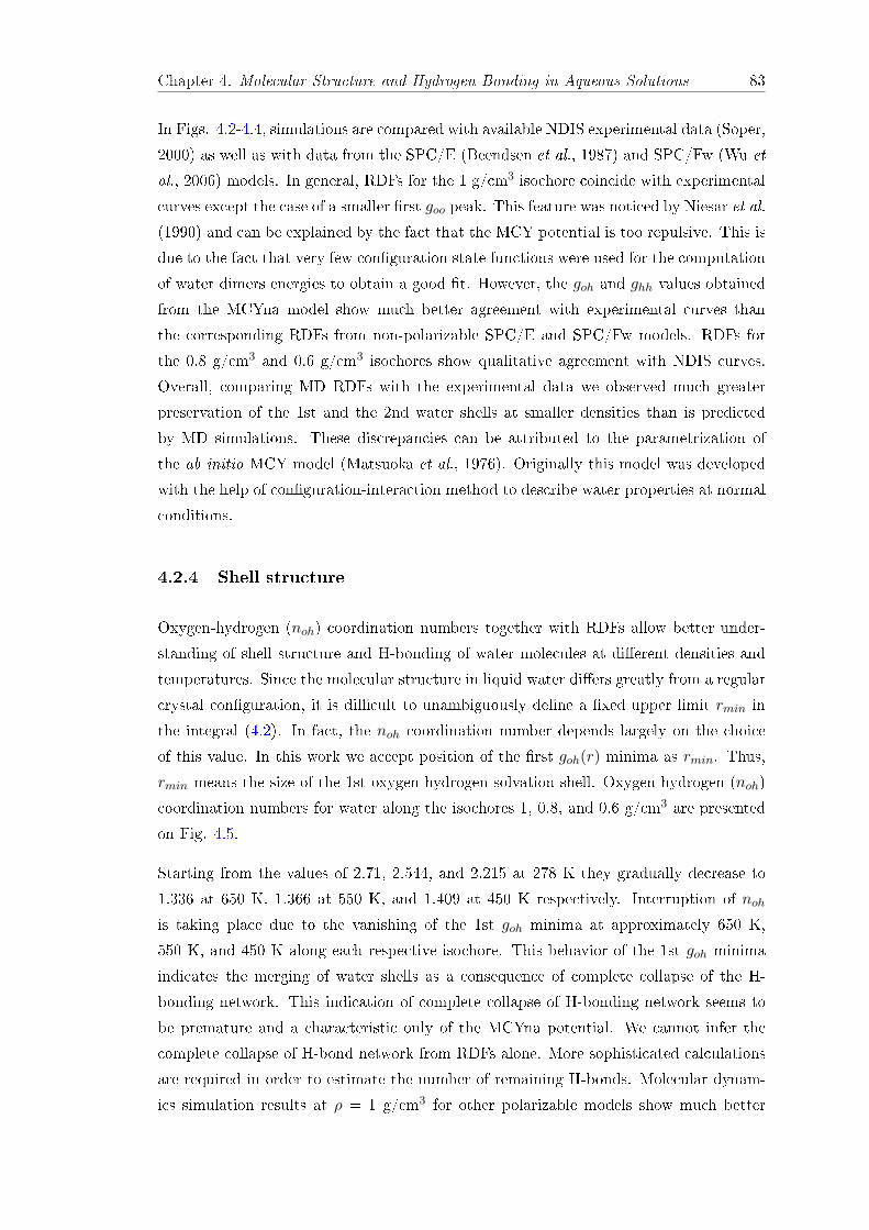
Chapter 4. Molecular Structure and Hydrogen Bonding in Aqueous Solutions 83
In Figs. 4.2-4.4, simulations are compared with available NDIS experimental data (Soper,2000) as well as with data from the SPC/E (Beendsen et al., 1987) and SPC/Fw (Wu etal., 2006) models. In general, RDFs for the 1 g/cm3 isochore coincide with experimentalcurves except the case of a smaller �rst goo peak. This feature was noticed by Niesar et al.(1990) and can be explained by the fact that the MCY potential is too repulsive. This isdue to the fact that very few con�guration state functions were used for the computationof water dimers energies to obtain a good �t. However, the goh and ghh values obtainedfrom the MCYna model show much better agreement with experimental curves thanthe corresponding RDFs from non-polarizable SPC/E and SPC/Fw models. RDFs forthe 0.8 g/cm3 and 0.6 g/cm3 isochores show qualitative agreement with NDIS curves.Overall, comparing MD RDFs with the experimental data we observed much greaterpreservation of the 1st and the 2nd water shells at smaller densities than is predictedby MD simulations. These discrepancies can be attributed to the parametrization ofthe ab initio MCY model (Matsuoka et al., 1976). Originally this model was developedwith the help of con�guration-interaction method to describe water properties at normalconditions.
4.2.4 Shell structure
Oxygen-hydrogen (noh) coordination numbers together with RDFs allow better under-standing of shell structure and H-bonding of water molecules at di�erent densities andtemperatures. Since the molecular structure in liquid water di�ers greatly from a regularcrystal con�guration, it is di�cult to unambiguously de�ne a �xed upper limit rmin inthe integral (4.2). In fact, the noh coordination number depends largely on the choiceof this value. In this work we accept position of the �rst goh(r) minima as rmin. Thus,rmin means the size of the 1st oxygen-hydrogen solvation shell. Oxygen-hydrogen (noh)coordination numbers for water along the isochores 1, 0.8, and 0.6 g/cm3 are presentedon Fig. 4.5.
Starting from the values of 2.71, 2.544, and 2.215 at 278 K they gradually decrease to1.336 at 650 K, 1.366 at 550 K, and 1.409 at 450 K respectively. Interruption of noh
is taking place due to the vanishing of the 1st goh minima at approximately 650 K,550 K, and 450 K along each respective isochore. This behavior of the 1st goh minimaindicates the merging of water shells as a consequence of complete collapse of the H-bonding network. This indication of complete collapse of H-bonding network seems tobe premature and a characteristic only of the MCYna potential. We cannot infer thecomplete collapse of H-bond network from RDFs alone. More sophisticated calculationsare required in order to estimate the number of remaining H-bonds. Molecular dynam-ics simulation results at ρ = 1 g/cm3 for other polarizable models show much better

Chapter 4. Molecular Structure and Hydrogen Bonding in Aqueous Solutions 84
270 300 330 360 390 420 450 480 510 540 570 600 630 660 690 720 750
1.4
1.6
1.8
2.0
2.2
2.4
2.6
2.8
3.0
1 g/cm3
0.6 g/cm3 0.8 g/cm3
Coo
rdin
atio
n nu
mbe
r nO
H(T
)
T[K]
1 g/cm3
Figure 4.5: Evolution of the �rst oxygen-hydrogen coordination numbers with tem-perature along the 1, 0.8, and 0.6 g/cm3 isochores. Comparison is between MCYna
(circles), SPC/E (crossed squares), and SPC/Fw (crossed diamonds).
conservation of H-bond structure. For example, according to the ab initio simulation ofKang et al.(2011) the tetrahedral H-bond network exhibits collapse above 800 K whereascalculation with TIP4P model (Mountain, 1989) indicates that 70% of hydrogen bondsstill remain at temperatures up to 1130 K. The number of hydrogen bonds obtained fromnon-polarizable models like SPC/E (see Fig. 4.5) keep gradually decreasing well beyond650 K. According to the MCYna potential, at T ≥ 650 K (ρ = 1 g/cm3), almost halfof the H-bonded molecules transform to be interstitial molecules. The reason for thediscrepancy between the potential models is due to the de�nition of hydrogen bond. It isimportant to note that the noh coordination number is not exactly the number of hydro-gen bonds. Eq. (4.5) de�nes average number of molecules, which lie within a distancermin from the central water molecule. As was shown by Kalinichev and Bass (1994), thisnumber coincides with number of H-bonds only at T ≤ 500 K. At higher temperaturesand pressures geometrical criteria alone used in Eq. (4.5) are not su�cient. More elab-orate criteria are required for the de�nition of H-bonds over wider range of state points(Yoshii et al., 2011; Kalinichev and Bass, 1994). Taking such factors into considerationand despite the fact the quantitative assessment of the degree of hydrogen bonding isstill a matter of debate, we can say that in real water at least some part of H-bond net-work still exists even at supercritical temperatures. The evaluation of oxygen-hydrogencoordination numbers along the 1g/cm3 isochore has also been performed for the rigid

Chapter 4. Molecular Structure and Hydrogen Bonding in Aqueous Solutions 85
SPC/E and �exible SPC/Fw models. The comparison with the �exible water model isparticularly important at high temperatures when the energy of intermolecular vibrationsis comparable with kBT. Incorporation of �exibility is intended to produce more realisticdynamic behavior of hydrogen bonds. It is apparent from Fig. 4.5 that these modelsgive values of noh higher by approximately 0.4 and keep gradually decreasing well beyond650 K. Introduction of bond �exibility does not signi�cantly noh change compared to therigid SPC/E model. However, as discussed above, SPC based models overestimate thewater structure, resulting in a 1st OH peak that is too high and an unrealistically sharpseparation between the water shells, especially at lower densities. Taking into accountthe comparison between MD and experimental RDFs from Figs. 4.2 - 4.5, it is apparentthat the MCYna model yields more accurate noh values than the SPC-based models. Itis also important to note that at lower densities it is di�cult to calculate reliable noo
and noh for non-polarizable water models due to strong local density �uctuations.
We also calculated oxygen-oxygen coordination numbers (noo) along the isochores 1,0.8, and 0.6 g/cm3 (see Table 4.1). In the 278-373 K temperature region the noo havevery similar values, only increasing slowly with an increase on temperature. Along the1 g/cm3 isochore noo starts from the classical value of 4.6 at 278 K and increases toapproximately 4.9 at T = 373 K. For the 0.8 g/cm3 isochore noo increases from 4.076to 5.5. For the 0.6 g/cm3 isochore noo has values from 3.7 at 278 K to 4.5 at 373 K.The closeness of these coordination numbers in this temperature region indicates thepresence of tetrahedral structure in water along the isochore 0.8 and possibly 0.6 g/cm3.However, in the temperature region shortly after normal boiling temperature and untilapproximately 400 K a very sharp rise in the noo values occurs. After 400 K, noo slowlydecreases to values of 12∼13 at supercritical temperatures (John and Eyring, 1975). Thereason for this discontinuity in noo values can be seen in the temperature dependence ofoxygen-oxygen RDFs. In this region of intermediate temperatures these RDFs (goo) showcharacteristics that are speci�c to only the MCYna model. As is clearly seen from the goo
values in Fig. 4.2 the 2nd peak, which represents the second coordination shell, vanisheswith increased temperature and pressure. This indicates that the �rst two coordinationshells are merging into one shell with much more closely packed molecular structure.Merging shells make impossible proper determination of the integration limit rmin (seeEq. (4.2)). The positions of the �rst O-O and O-H minima along the 1, 0.8, and 0.6g/cm3 isochores are presented in the Table 4.1. Many authors (Yoshii et al., 1998; Kanget al., 2011; Mountain, 1989) take positions of the 1st OO and OH minima at 25◦C ascriteria of H-bond forming. However, as is apparent from the data in Table 4.1, thesepositions are not �xed but are temperature and density dependent. This e�ect imposesadditional uncertainty on the choice of H-bond criteria.

Chapter 4. Molecular Structure and Hydrogen Bonding in Aqueous Solutions 86
Table4.1:
Posit
ions
ofthe�rst
minim
aof
theMCY
naRD
Fstogether
with
noovalues
alon
gthe1,
0.8,
and0.6g/
cm3iso
chores.
1g/
cm3
0.8g/
cm3
0.6g/
cm3
T[K]
O-O
r min
[Å]
noo
O-H
r min
[Å]
O-O
r min
[Å]
noo
O-H
r min
[Å]
O-O
r min
[Å]
noo
O-H
r min
[Å]
298
3.37
54.60
52.41
93.56
64.33
72.57
13.74
23.86
92.57
434
33.43
74.91
22.41
93.66
74.82
42.53
83.81
64.11
12.57
437
33.46
85.09
02.41
93.69
95.04
02.50
43.88
84.37
42.57
445
0-
-2.35
8-
-2.43
84.21
75.95
22.46
450
04.76
314
.560
2.35
84.72
712
.790
2.33
94.47
37.04
3-
550
4.67
013
.561
2.32
74.72
711
.989
2.27
24.69
28.23
0-
650
4.60
813
.021
2.17
34.79
411
.939
-4.98
49.51
3-
750
4.60
813
.009
-4.82
712
.173
-4.94
79.53
2-

Chapter 4. Molecular Structure and Hydrogen Bonding in Aqueous Solutions 87
4.3 Molecular structure and hydrogen bonding in aqueousnonpolar solute mixtures
As was discussed in Chapter 2, the interaction of nonpolar solutes with water is ac-companied by many unusual changes in water structure and thermodynamic properties(Chaplin, 2013; Ball, 2008). This kind of interaction has the generic name "hydrophobicinteraction" and hydration of nonpolar solutes is called "hydrophobic hydration". Theterm "hydrophobic interaction" refers to the structural and energetic response of waterin the vicinity of hydrophobic solutes as shown on Figure 2.9 in Chapter 2. It describesthe interaction of nonpolar molecules with water, each other and the interaction betweenwater molecules in the presence of two or more nonpolar molecules. The "hydrophobice�ect" of hydrophobic solutes in water (such as non-polar gases) is primarily a conse-quence of changes in the clustering in the surrounding water rather than water-soluteinteractions (Fisicaro et al., 2010). In this chapter the calculation of aqueous nonpolarsolutes is performed with the help of combined MCYna + LJ potential model (see Eqs.(2.4 - 2.7), Chapter 2) and the Lorentz-Berthelot combination rules (see Eqs. (2.12),Chapter 2). The Lennard-Jones parameters ε and σ of neon, argon, methane, krypton,and xenon are given in Table 4.2.
Table 4.2: Lennard-Jones potential parameters used for water-solute and solute-solutepair interactions (Guillot and Guissani, 1993).
ε/kb [K] σ [nm]H2O 78.22 (O) 0.3136 (O)Ne 18.56 0.3035Ar 125.0 0.3415CH4 147.5 0.3730Kr 169.0 0.3675Xe 214.7 0.3975
Below we present results fromMD simulations of water-neon, -argon, -methane, -krypton,and -xenon mixtures at solute molar fractions xs = 1 − 30% in the single phase regionand temperature range 298-750 K.
4.3.1 Water-solute radial distribution functions
To de�ne the inner structure of these systems we studied RDFs at 298 K and xs =20% for Ne and Ar, xs = 15% for CH4, xs = 10% for Kr and 6% for Xe. Fig. 4.6shows solute-oxygen (gso) radial distribution functions. From this �gure we can seethat the solute-oxygen curves start at distances proportional to the parameter σ, in the

Chapter 4. Molecular Structure and Hydrogen Bonding in Aqueous Solutions 88
following order σNe < σAr < σCH4 < σKr < σXe. The position of the 1st peaks allowsus to identify the radius of the 1st solvation shell water molecules form around soluteparticles. The approximate radii for the given values of xs and temperature are: rNe
= 0.313, rAr = 0.332, rCH4 = 0.334, rKr = 0.35, and rXe = 0.365 nm. Simulationsperformed for higher temperatures show that the size of the solvation shells decreaseslightly with increasing temperature. One of the main tasks of the present work wasto investigate the distortion of the structure of water caused by the inert solutes. Fig.4.7 compares oxygen-oxygen (goo), oxygen-hydrogen (goh), and hydrogen-hydrogen (ghh)RDFs for pure water with RDFs of water-Ne, water-Ar, and water-CH4 systems at T =298 K and xs = 20%. It is apparent from Fig. 4.7 that the presence of the nonpolar soluteincreases and slightly widens the 1st O-O, O-H, and H-H peaks. Water-argon and water-methane O-O and O-H �rst peaks are higher than in the case of pure water (dash curve).We can conclude that increasing the concentration of a large nonpolar solute particlelike Ar or CH4, compresses the water structure because of solute-oxygen repulsion. Thesecond O-O peak is �attening out and almost disappears in the presence of 15 - 20%solute particles, which indicates a signi�cant distortion of the usual water shell structureby solute particles at distances larger than 4 nm. The e�ect of the solutes on goh(r) isto increase the 1st minima and decrease the 2nd minima. In general, data from Fig. 4.7suggest that the solute particles slightly distort the 1st shell while the distortion of waterstructure at longer distances is much more signi�cant. Similar indications of nonpolarsolutes induced distortion of water structure were obtained for dilute aqueous mixturesof Ar (Botti et al., 2003; Alagona and Tani, 1980), CH4 (Okazaki et al., 1979), He (Bottiet al., 2003), and Kr (Botti et al., 2003).
By analyzing the distribution functions from Figs. 4.6 and 4.7 we can infer the shape ofthe solvation shell around solute particles. For example, by comparing the 1st Ne-O andNe-H peaks positions we can see that the 1st Ne-H peak is located some 0.95 nm closerto the Ne atom than the 1st Ne-O peak, which is almost equal to the length of O-Hcovalent bond (0.9752 nm for the MCYna model). Taking this into account, we can inferthat the hydrogen atoms of the water molecules, which form a shell around Ne atoms,are oriented almost radially inward. This orientation of H-atoms is in agreement withthe Hartree-Fock calculations of Losonczy et al., (1973) which indicate that the water-neon pair potential has a minimum when the Ne atom is located in the water moleculeplane along one of the O-H axes. RDFs for larger solute particles show similar behavior.The hydrogen atoms of water molecules in the 1st solvation shell are orientated slightlytoward the central solute particle, however, not completely radially like it is in the caseof the small Ne atom.
The 2nd peaks of gArO(r), gCH4O(r), gKrO(r), and gXeO(r) are located at a shorterdistance than the 2nd peaks of the corresponding solute-hydrogen functions (0.615 nm

Chapter 4. Molecular Structure and Hydrogen Bonding in Aqueous Solutions 89
0.0 0.1 0.2 0.3 0.4 0.5 0.6 0.7 0.8
0.0
0.5
1.0
1.5
2.0
2.5
3.0
g SO(r
)
r [nm]
Figure 4.6: Solute-oxygen gso(r) RDFs for water-solute systems at 298 K. Startingfrom left to the right, the solutes are Ne (black xs = 20%), Ar (red xs = 20%), CH4
(green xs = 15%), Kr (blue xs = 10%), and Xe (olive xs = 6%).
for Ar-O vs. 0.64 nm for Ar-H, 0.638 nm for CH4-O vs. 0.66 nm for CH4-H, 0.62 nm forKr-O vs. 0.665 nm for Kr-H, and 0.583 nm for Xe-O vs. 0.63 nm for Xe-H for the valuesof xs indicated in Fig. 4.6). This means that the water molecules of the 2nd shell pointtheir oxygen atoms preferentially towards the solute and the hydrogen atoms towardsthe bulk, while in the 1st shell H atoms are pointed from the bulk and toward the soluteparticle. This enclathration mechanism, or encagement phenomenon, has been viewed inseveral simulation studies (Shvab and Sadus, 2012b; De Grandis et al., 2003; Cristoforiet al., 2005; Alagona and Tani, 1980) on hydrophobic solutes in water and it is one ofthe most important feature of hydrophobic hydration at the atomic level.
4.3.2 Structure of the solvation shells
We studied the evolution of water-nonpolar solute solvation shells using the water-argonsystem as the example. Aqueous solutions of CH4 and Ne have similar phase behavior atxs ≤ 30% and exhibit similar temperature dependence of the solvation shells. Fig. 4.8presents the 1st order coordination numbers for water-argon system calculated by Eq.(4.2). Since the molecular structure in liquid water di�ers from a regular con�gurationof crystal as in ice, it is di�cult to unambiguously de�ne a �xed upper limit rmin inintegral (4.2). In fact, the coordination number nij depends largely on the choice of this

Chapter 4. Molecular Structure and Hydrogen Bonding in Aqueous Solutions 90
0.0 0.1 0.2 0.3 0.4 0.5 0.6 0.7 0.8
0.0
0.5
1.0
1.5
0.0
0.5
1.0
1.5
0.0
0.5
1.0
1.5
2.0
2.5
g HH(r)
r [nm]
(c)
(b)
g OH(r)
g OO(r)
(a)
Figure 4.7: Oxygen-oxygen, oxygen-hydrogen, and hydrogen-hydrogen distributionfunctions of pure water (dashed black line) and aqueous solutions of Ne (short dashedline xs = 20%), Ar (dotted red line xs = 20%), and CH4 (continuous green line xs =
15%) at T = 298 K.
value. In this work we accept the position of the �rst gij(r) minima as a rmin. Thus,rmin represents the size of the 1st solvation shell. Each curve in Fig. 4.8a represents theargon-oxygen coordination number nArO or the so-called hydration number at di�erentxs in the one phase region. In general, nArO slowly decreases with temperature reachingstable values at T ≥ 650 K. At argon mole fractions ≤ 20% and T < 400 K the number ofwater molecules forming a solvation shell around an argon atom is approximately 15∼17and slowly decreases to 14 at supercritical temperatures. This compares with hydrationvalues of 15∼14 for water-neon (xs = 20%), 16∼17 for water-methane (xs = 20%), 18for water-krypton (xs = 10%) and 19∼20 for water-xenon (xs = 6%). These values liewithin the range of hydration numbers reported in the literature (Okazaki et al., 1979;Dec et al., 2006).
The oxygen-oxygen coordination numbers noo for water-argon systems are presented inFig. 4.8b. At temperatures up to the normal boiling temperature, the presence of Aratoms increases noo. For example, the generally accepted value of noo for pure water at

Chapter 4. Molecular Structure and Hydrogen Bonding in Aqueous Solutions 91
298 K is 4.6 whereas at xs = 10% it is 5.1 and for xs = 20% it is 5.96. This increasein the number of water molecules inside the 1st coordination shell can be explained bythe formation of a more densely packed H-bond network due to signi�cant repulsionfrom Ar atoms. Con�rmation of this e�ect is explicitly seen in Fig. 4.7b where the �rstsolute-oxygen peaks at solute concentrations of 20% are clearly higher than that of purewater. This is possible in part because of the incorporation of water molecules fromthe 2nd shell into the 1st one. Our simulations show that at temperatures up to theboiling temperature values of noo at xs = 10% are close to noo of pure water. Naturally,with increasing number of Ar atoms the tetrahedral water structure becomes increasinglydistorted until at some point it collapses completely. By analyzing values of noo withhigher solute concentrations we can infer that the tetrahedral structure collapses at soluteconcentrations > 20%.
14
15
16
17
6
8
10
12
14
300 350 400 450 500 550 600 650 700 750
1.5
2.0
2.5
3.0
nArO
nOO
nOH
T [K]
Figure 4.8: Temperature dependence of (a) argon-oxygen, (b) oxygen-oxygen, and (c)oxygen-hydrogen coordination numbers at argon mole fractions of 0% (black ¥), 10%
(red N), 20% (blue ©), and 30% (green H).

Chapter 4. Molecular Structure and Hydrogen Bonding in Aqueous Solutions 92
The evolution of the oxygen-hydrogen coordination number (noh) of the water-argonsystem is the most interesting one. The O-H coordination numbers for xs = 10, 20, and30% together with corresponding values for pure water are presented in Fig. 4.8c. Wehave calculated these coordination numbers using Eq. (4.2) which requires the positionof the O-H 1st minima as an upper integration limit. It is important to note that thenoh coordination number is not exactly the number of hydrogen bonds. Eq. (4.2) de�nesthe average number of molecules which are within a distance rmin from the centralwater molecule. As was shown by Kalinichev and Bass (1994) this number coincideswith the number of H-bonds only at T ≤ 500 K. At higher temperatures and pressuresmore elaborate criteria are required for the de�nition of H-bonds over a wider range ofstate points. Nevertheless, noh can serve as a good approximation of H-bond number,especially at T ≤ 500 K. As we can clearly see from Fig. 4.8c the presence of Aratoms increase noh. Many authors (Guillot and Guissani, 1993; Alagona and Tani, 1980;Okazaki et al., 1979) suggest that small concentrations of inert solutes strengthen thewater structure by increasing the number of H-bonds in the �rst hydration shell.
Analyzing the data from Figs. 4.7a, and b and 4.8c we can infer that some short-rangestrengthening of the H-bond network in the vicinity of the solute particle occurs insystems with xs ≤ 30%. However, at the same time, the data from Figs 4.7a, and balso show a negative in�uence of nonpolar solutes on the structuring of water moleculesin the second hydration shell, especially at xs ≥ 20% and at distances larger than 4nm from the solute particle. The noh values at xs = 30, 20, and 10% are higher thanthat of pure water at T < 400 K. In the region 400 - 450 K a signi�cant drop in noh
is observed and after T = 450 K all oxygen-hydrogen coordination numbers merge intoone and have values that are very close to that of pure water. At T < 400 K, where thetetrahedral structure still exists, the increase in noh can be explained by the formation ofa more densely packed solvation shell due to repulsion from solute atoms. The noh curveis interrupted at 650 K where the 1st goh minimum disappears. At this temperaturethe 1st and 2nd O-H shells merge and it becomes di�cult to unambiguously de�ne a�xed upper limit rmin in integral (4.2). We believe that more than half of the H-bondnetwork breaks at T ≥ 650 K. In the case of xs > 30% irrespectively of solute size, thesolute particles largely block water molecules from forming either H-bonds or any kindof cluster formations.
Fig. 4.9 presents coordination numbers of water plus Ne, Ar, CH4, Kr, and Xe sys-tems at 298 K as a function of solute concentrations. This �gure can be interpreted asthe dependence of coordination numbers on the size of the solute particles. All threecoordination numbers solute-oxygen, oxygen-oxygen, and oxygen-hydrogen show a cleardependence on the σ parameter of solute particles. Coordination numbers from Fig.4.9 follow the dependence σXe > σKr > σCH4 > σAr > σNe. This dependence has a

Chapter 4. Molecular Structure and Hydrogen Bonding in Aqueous Solutions 93
13
14
15
16
17
18
19
4.5
5.0
5.5
6.0
6.5
2 4 6 8 10 12 14 16 18 20 22 24 26 28 302.6
2.7
2.8
2.9
3.0
3.1
n SO
n OO
n OH
xS[%]
Figure 4.9: Coordination numbers of aqueous solutions of Ne (black ¨), Ar (red ©),CH4 (green N), Kr (blue ¥), and Xe (olive H) at T = 298 K as a function of solute
concentration.
very simple explanation, larger particles require larger solvation shell, smaller particles -smaller shell. noo and noh start from values close to that of pure water at small xs andincrease with increasing solute concentrations. In contrast to noo and noh solute-oxygencoordination numbers nso decrease with increasing solute concentrations.
We have compared the internal energies of pure water and water-argon mixtures withargon concentrations 2, 6, 10, and 20% at the same number densities and at T = 298K. The internal energy of the 2% water-argon system is smaller by -3.181 kJ/mol thanthat of pure MCYna water. This result is in agreement with the results from Okazaki etal. (1979) and Alagona and Tani (1980) and indicates energetic stabilization of vicinalwater molecules by solute atoms. However, at higher concentrations, even at xs = 6%,the water-argon internal energy becomes larger than in pure water, gradually increasingwith xs. This change in internal energy can be explained by the cost of incorporating

Chapter 4. Molecular Structure and Hydrogen Bonding in Aqueous Solutions 94
argon atoms into the H-bond network. Only in very dilute mixtures can the few so-lute atoms be easily incorporated into the existing water tetrahedral structure withoutcausing signi�cant perturbation. At higher xs, solute atoms cause more and more per-turbations to the structure of water. Despite the somewhat strengthening e�ect on the1st surrounding water shell (mainly more dense packing of water molecules), excessivenumbers of solute particles destabilize the cohesiveness of the water structure.
4.3.3 One-phase region
All simulation data for water and aqueous solutions presented in this work belong to thesingle-liquid phase region at constant density 1g/cm3. Knowing the very small solubilityof nonpolar gases like Ne, Ar, Kr, Xe, and CH4 in water (Kennan and Pollack, 1990)at ambient and near ambient conditions one may naturally question the stability of thephase state.
Solute concentration and size also a�ect the solubility of the given substances in water.Our simulations indicate a tendency for the large Xe and Kr atoms to demix at con-centrations higher than 6% and 10%, respectively. Medium sized Ar and CH4 tend todemix at xs > 30% while small Ne atoms remain in a single phase with water even athigher concentrations. The solubility of these particles also depends on temperature. Atxs ≤ 10% all the water-solutes systems appear to be in one phase throughout the entiretemperature region of 278 - 750 K irrespective of the size of the solute particles. Atambient temperatures, both water-Ar and water-CH4 systems separated into two phaseswhen xs = 20%. At xs = 30% water-argon and water-methane systems do not tend tomix at temperatures up to 340 K and 450 K respectively. Therefore, all results presentedin the given work belong to the ranges of xs and temperature where full water-solutemiscibility is attained.
We report calculations for the homogeneous phase at elevated temperatures, involvingsolute concentrations up to 30%. These phase conditions obtained at constant volume(NVT ensemble) should not be confused with the very small solubility of noble gasesand methane in water at ambient conditions. Extensive experimental studies of variousaqueous solutions of nonpolar solutes conducted by Franck et al. (1974) con�rm theexistence of a single homogeneous phase at xs = 30% and even higher concentrationsat near critical and supercritical temperatures. For example, Fig. 10 in Franck (1987)and Fig. 2 in Wu et al. (1990) clearly show phase equilibrium isopleths and isothermsat solute concentrations up to 30% at near critical temperatures for water-methane andwater-argon systems, respectively. Although the existence of a single phase for watermixtures of relatively high non-polar solute concentrations (xs ≥ 30%) has been observed

Chapter 4. Molecular Structure and Hydrogen Bonding in Aqueous Solutions 95
experimentally at high temperatures and high pressures, the extent of miscibility at lowtemperatures (T < 500 K) and high pressures remains unclear.
The very low methane solubility in water at T < 500 K and p < 100 MPa has beenamply demonstrated by both experimental (Franck, 1987; Wu et al., 1990; Japas andFranck, 1985; Zheng et al., 2012) and simulation data (Errington et al., 1998). However,most measurements have been reported for the methane in the gas state, e.g., a density of0.00068 g/cm3 at T = 288 K, p = 0.1 MPa. In contrast, for the NVT simulations reportedhere, the density of the whole mixture is held constant at 1g/cm3, which is more than 1000times larger than reported by Zheng et al. (2012) and Errington et al. (1998). As a resultof this con�nement, the pressures observed in our simulations are much higher, resultingin increased solubility. For example, our pressures at the same methane concentrationsreported in by Errington et al. (1998) (Figs. 4.6 - 4.9) are greater than 200 MPa (423K), 420 MPa (523 K), and 600 MPa (603 K). This compares with pressures less than100 MPa at low methane concentration at these temperatures (Errington et al., 1998).In the work of Culberson and McKetta (1951) (Fig. 2), a pressure-composition diagramfor methane + water is reported based on some experimental observations at 298 K. Itshould be noted that this diagram is at best semi-quantitative, and as such considerablecaution should be exercised in its use. Nonetheless, with this important caveat in mind,it appears to identify a single-phase liquid region for methane concentrations of up to15% and pressures up to 1 GPa.
To check the stability of the mixtures, we conducted additional simulations for water-neon and water-methane at xs = 20% and 30% using boxes elongated two-fold in onedirection with the clearly separated water-rich and solute-rich phases. We also comparedthe miscibility range of the MCYna + LJ system with that of the nonpolarizable SPC/E+ LJ model. In the elongated simulation box, all systems were equilibrated for 1 nswith another 1 ns dedicated for accumulation of ensemble averages. All systems showedthe same mixing behavior as in the original cubic simulation box with the same valuesof dielectric constant and dipole moment. We found that the single homogeneous phasefor the nonpolarizable SPC/E + LJ system is restricted to smaller solute concentrationsthan can be observed for the MCYna + LJ system. For water-methane, the highestsolute concentrations at which a single phase was obtained using SPC/E + LJ are xs =20% at T > 650 K and xs = 15% at T > 400 K. For the water-Ne system the highestsingle-phase conditions are xs = 30% at T > 650 K and xs = 20% at T > 400 K. Incontrast, the MCYna + LJ calculations yield a single phase at solute concentrations upto 30% for both systems. As the solute particles are modeled by the same LJ potential,the di�erences observed can be attributed to the water potential. The average MCYnawater-water intermolecular energy is -39.0 kJ/mol, which compares with a value of -47.0kJ/mol for the SPC/E potential. This suggests that the more loosely attracted, MCYna

Chapter 4. Molecular Structure and Hydrogen Bonding in Aqueous Solutions 96
water molecules allow solute particles to di�use inside the hydrogen-bond network to agreater extent than SPC/E water molecules. Di�erences in the structure of water ob-tained by the two di�erent potentials are apparent in the oxygen-oxygen RDFs (Shvaband Sadus, 2012a). The SPC/E O-O peak reaches value 3.2 at T = 298 K while theMCYna O-O peak has a value of 2.5. This again indicates a much more strongly con-nected water shell structure of the SPC/E model. As shown elsewhere (Shvab and Sadus,2012a) SPC/E provides better prediction of water's structure at T < 373 K, while sig-ni�cantly overestimating its structure at T > 373 K, particularly at low densities. TheMCYna model underestimates water molecules ordering at ambient conditions, but atthe same time it is much better in predicting the dielectric constant, dipole moment, andto some extent hydrogen bonding (see Figs. 2-4 in (Shvab and Sadus, 2012a)), which areproperties of interest in this work.

Chapter 5
Polarization Properties of AqueousNonpolar Solute Mixtures
The polarization properties of polar substances like water are usually described in termsof the dielectric constant and dipole moment (Fröhlich, 1958; Feldman et al., 2006;Böttcher et al., 1973). For most materials these quantities are independent of the strengthof the electric �eld over a wide range of the latter, but in the case of alternating �eldsdepend on the frequency. They also depends on parameters, such as the temperature,which de�ne the state of the material. In the macroscopic (phenomenological) theory,which will be summarized in the next paragraph, the dielectric constant is supposedto be known empirically. Throughout this work we shall be interested only in internalelectric �elds created by all water molecules in the system.
The simulation details were given in Chapter 4.
5.1 Current theories of dielectrics
In a dielectric, two essentially di�erent types of interaction forces should be distinguished.Forces due to chemical bonds, van der Waals attraction, repulsion forces, and othersare all short ranged, and usually interactions between nearest neighbors only need beconsidered. Comparing with these interactions, dipolar interaction forces have a verylong range (Fröhlich, 1958). Water is a strong dielectric with dielectric constant ε =78.65 at 25◦C and 0.1 MPa, and the dipole moment µ ≈ 2.2 - 3 D. Due to the longrange nature of the dipolar forces an accurate calculation of dipole-dipole interactionis complicated. Here we present major theories of polarization properties of water and
97

Chapter 5. Polarization Properties of Aqueous Nonpolar Solute Mixtures 98
binary mixtures, and formulas for dielectric constant and dipole moment applicable formolecular dynamic simulations.
When a body is placed in a uniform electric �eld Eo in vacuum, caused by a �xed chargedistribution, its dipole moment will in general change. The di�erence between the dipolemoments before and after the application of the �eld Eo is called the induced dipolemoment µind, and the body in this case is called polarizable (Böttcher et al., 1973). Inmost cases polarizable bodies are polarized linearly, that is, the induced moment µind isproportional to Eo. In this case one has
µind = αE0, (5.1)
where ε is the dielectric constant, α is the polarizability of the body and a scalar quan-tity. The fundamental equation which de�nes the dielectric constant ε from the internalelectric �eld inside any dielectric material is given by (Fröhlich, 1958; Feldman et al.,2006)
ε− 14π
E =∑
k
Nk
[αk(Ei)k +
µ2k
3kT(Ed)k
], (5.2)
where summation is over all species k and Ei is the internal electric �eld. It is de�ned asthe total electric �eld at the position of the particle minus the �eld due to the particleitself. In Eq. (5.2) the Ed is a so-called directing �eld, part of the total electric �eldE tending to direct the permanent dipoles µk. For a nonpolar system the fundamentalequation for the dielectric constant is simpli�ed to the famous Clausius-Mosotti formula(Fröhlich, 1958)
ε− 1ε + 2
=4π
3
∑
k
Nkαk. (5.3)
In this case, only the relation between the internal �eld Ei and the Maxwell �eld E hasto be determined. In old Debye theory the internal �eld Ei and directing �eld Ed werenot distinguished from each other. Insteed of both �elds in the square brackets in Eq.(5.2), Debye used the Lorentz �eld EL.
EL =ε + 2
3E. (5.4)
Substituting this expression into Eq. (5.2) we can �nd

Chapter 5. Polarization Properties of Aqueous Nonpolar Solute Mixtures 99
ε− 1ε + 2
=4π
3
∑
k
Nk
[αk +
µ2k
3kT
]. (5.5)
This is generally called the Debye equation (Fröhlich, 1958; Feldman et al., 2006). It wasthe �rst relationship that made the connection between the molecular parameter of thesubstance being tested and the phenomenological (macroscopic) parameter that can beexperimentally measured. It works well for gases at normal pressures. However, in manyother cases the Debye equation is in considerable disagreement with the experiment.
In the case of spherical molecules Onsager has shown that it is possible to go one stepfurther in the approximate calculation of the dielectric constant (Fröhlich, 1958). Theinteraction between molecules will no longer be entirely neglected, but one component ofit, namely the long-range dipolar interaction, will be taken into account. The followingassumptions are made (Fröhlich, 1958; Feldman et al., 2006):
• A molecule occupies a sphere of radius a and its polarizability is isotropic;
• The short range interaction energy is negligible (i.e. ¿ kT per molecule).
As was shown above, when a molecule with permanent dipole strength µ is surroundedby other particles, the inhomogeneous �eld of the permanent dipole polarizes its envi-ronment, and as aconsequence, orientation of the dipole moment is in�uenced. A simplemodel has been proposed to calculate this e�ect: an ideal dipole in a center of a sphericalcavity. The �eld of the dipole in such a cavity polarizes the surrounding matter, whichin turn gives rise to a so-called reaction �eld R. It can be shown that the the reaction�eld R is
R =1
2ε+12(ε−1) − α
a3
µ
a3, (5.6)
where a is the radius of the cavity. The internal �eld is now given by
Ei = Ed + 〈R〉 , (5.7)
where 〈R〉 is is the average reaction �eld connected with the permanent part of the dipolemoment µ. Taking into account Clausius-Mossotti formula (5.3) for polar systems inhigh-frequency alternating �elds (Fröhlich, 1958; Feldman et al., 2006):
ε∞ − 1ε∞ + 2
=4π
3
∑
k
Nkαk, (5.8)

Chapter 5. Polarization Properties of Aqueous Nonpolar Solute Mixtures 100
and performing further algebraic transformations we can get
(ε− ε∞)(2ε + ε∞)ε(ε∞ + 2)2
=4πρ
9kTµ2, (5.9)
where ρ is the number density and the ε∞ is the dielectric constant at a frequency atwhich the permanent dipolescan no longer follow the changes of the �eld but where theatomic and electronic polarization are still the same as in static �elds. For most naturalmateraials ε∞ ≈ n2, where n is the optical refractive index. The Eq. (5.9) is generallycalled the Onsager equation (Fröhlich, 1958; Feldman et al., 2006).
Kirkwood applied methods of statistical mechanics to �nd macroscopic quantities whenthe properties of the molecules and the molecular interactions are known. The electricpolarization P is de�ned as P = D − ε0E, where D is the electric displacement �eldinside some material, and ε0 is the permittivity of vacuum. When the higher multipoleinteractions may be neglected the electronic polarizability P is equal to dipole density:
PV = 〈M〉 , (5.10)
where V is the volume of the dielectric under consideration an 〈M〉 is its statisticalmechanical average of the total dipole moment. In case of isotropic system the D = εE.Thus we can write (Fröhlich, 1958; Feldman et al., 2006):
(ε− 1)E =4π
V〈M〉 , (5.11)
Using statistical mechanics distribution functions for total dipole moment M =∑
µ inthe end we obtain famous Kirkwood equation for dielectric constant
ε− 1 =4πρµ2
3kTgk, (5.12)
where µ is the permanent dipole of a molecule and gk is the so-called Kirkwood factor.This factor can be obtained from the �uctuation of the total dipole moment of the system
gk =
⟨[∑Ni=1
(µi + µind
i
)]2⟩
Nµ2=
⟨M2
⟩
Nµ2, (5.13)
where⟨M2
⟩is the ensemble average of the square total dipole moment of the system.
The total molecular dipole moment µm which has contributions from both the partial

Chapter 5. Polarization Properties of Aqueous Nonpolar Solute Mixtures 101
charge permanent electric dipole µi and the induction interaction µindi , is averaged over
the entire molecular system. If there is no speci�c correlations one has gk = 1. If thedipole correlations are not negligible, more detailed information about the molecularinteractions is required in order to calculate gk (Neumann, 1983, 1986). The averagemolecular dipole moment is given by
µm =1N
N∑
i=1
(µi + µind
i
). (5.14)
In this work we are using polarizable MCYna water model described in Chapter 2. Theµind in this model is de�ned in Eqs. (2.7 - 2.9) from Chapter 2. Thus, having induceddipole moment we can calculate total dipole of a single molecule µm = µind + 2.1936.The 2.1936 D is the permanent dipole moment in the MCYna water model. Having totaldipole moment we can calculate dielectric constant of any polar liquid. In this workwe are using Kirkwood formula (5.12) to �nd dielectric constants of water and aqueoussolutions (Shvab and Sadus, 2012a, 2012b).
For the representation of a dielectric consisting of polarizable molecules with a permanentdipole moment, Fröhlich introduced a continuum with dielectric constant ε∞ in whichpoint dipoles with a moment µd are embedded. According to this model the polarizabilityof the molecules can be imagined as smeared out to form a continuum with dielectricconstant ε∞. After splitting polarization P into induced and orientational parts, andperforming necessary algebraic transformations Kirkwood formula (5.12) can be rewrittenin the following way
gkµ2 =
9kT
4π
(ε− ε∞)(2ε + ε∞)ε(ε∞ + 2)2
, (5.15)
where gk is the Kirkwood factor given by Eq. (5.13). Equation (5.15) is called theKirkwood-Frhölich equation, and it is used mainly for polar systems with short-rangeinteractions (Fröhlich, 1958; Feldman et al., 2006).
5.2 Polarization properties of bulk water
The dipole moment of an isolated water molecule in vapor is 1.85 D (Haynes et al., 2013).However, in condensed phases, the electrostatic �eld from the other molecules reorga-nizes the charge distribution in the molecule. The self-consistent induction calculationsgive an average total dipole moment of ice Ih 3.09 D (Batista et al., 1998). In the �uidphase, the dipole moment must have intermediate values between those in the gas and

Chapter 5. Polarization Properties of Aqueous Nonpolar Solute Mixtures 102
the ice. Therefore, it is not su�cient to describe the properties of water over a widerange of physical states based upon this kind of �xed-charge potential model. Instead,a realistic model should include the polarization e�ect of the molecule to describe theintermolecular interaction in the sub- and supercritical states. Car-Parrinello ab ini-tio MD (Car and Parinello, 1985) is one of the best methods to account for the statedependence of intermolecular interactions. Kang et al. (2011) and Dyer et al. (2006)reported a �rst principle study of sub- and supercritical water. These workers calcu-lated the structure factors and polarization distribution in water. However, the methodused is computationally expensive and involves a very small number of particles (32-64molecules). In this sense, we need simpler models to investigate the properties of waterover a wide range of thermodynamic states. A natural improvement of the empiricalpotential models is to explicitly introduce nonadditive many-body interactions such asthree-body and polarizable contributions. In this work we apply an ab initio MCYnapotential model for investigation of structural and polarization properties of bulk waterand compare results with available experimental data. This model was introduced by Liet al. (2007) and contains an ab initio description of two-body additive interactions plusnonadditive contributions from both three-body interactions and polarization. The non-additive multibody in�uence arises because the induced dipole of each molecule generatesan electric �eld that a�ects all other molecules. The molecular induced dipole momentsare determined self-consistently with the electrostatic �eld re�ecting the con�gurationof the �uid that depends on the physical state. A comparison is also made with SPC/Ewater model (Berendsen et al., 1987).
5.2.1 Dielectric constant
Molecular dynamics and experimental dielectric constants (Fernandez et al. 1997) arepresented in Fig. 5.1. As expected, εr is lower for higher temperatures. The temperaturedriven decrease of εr is due to the reduction of molecular ordering. One of the mainreasons for the high dielectric constant of water is that the extensive H-bond networkenables a fast (within 10 ps) reorientation of the molecular dipoles in response to a �eld.
Increasing the temperature increases the randomizing thermal �uctuations that opposedipole alignment by an electrostatic �eld. Values of the dielectric constant εr graduallydecrease along all isochores. The decrease of εr at lower densities is caused by stronglocal density �uctuations, and is a consequence of a broken H-bond network and reducedpolarizability of water.
Comparison with the experimental values of dielectric constant from elsewhere (Fernan-dez et al. 1997) shows that MCYna model underestimates εr by approximately 5% at

Chapter 5. Polarization Properties of Aqueous Nonpolar Solute Mixtures 103
270 300 330 360 390 420 450 480 510 540 570 600 630 660 690 720 750
10
20
30
40
50
60
70
80
90
0.6 g/cm3
0.8 g/cm3
r
T[K]
1 g/cm3
Figure 5.1: Temperature dependence of the dielectric constant εr. MD data alongthe 1, 0.8, and 0.6 g/cm3 isochores (all ©). A comparison is given with both directexperimental data (Fernandez et al. 1997) (open ¡) and interpolated experimental data
(Uematsu and Franck, 1980) (crossed ¢).
temperatures lower than 343 K, and overestimates εr for the temperatures greater than450 K. In the temperature range 343 - 450 K MCYna predictions and experimental dataalmost coincide. Experimental results for isochores 0.8 and 0.6 g/cm3 are available onlyin temperature regions 550 - 750 K and 630 - 750 K respectively. For lower temperatureswe used an interpolation equation based on the experimental data collected in the workof Uematsu and Franck (1980). In the case of smaller water densities, MD results deviatemore from experimental data than it was in case of ρ = 1 g/cm3.
Comparison with dielectric constants obtained from the SPC/E model is presented inTable 5.1. The MCYna model gives better agreement with experiment for tempera-tures up to 400 K than the SPC/E model, which can be at least partly attributed topolarization interaction. Above the critical temperature, both polarizable MCYna andnon-polarizable SPC/E models give similar values of the dielectric constant. This trendcan be explained by the fact that water at supercritical conditions behaves like simple�uid, due to the collapse of the shell structure and signi�cant reduction of the H-bondnetwork.

Chapter 5. Polarization Properties of Aqueous Nonpolar Solute Mixtures 104
Table5.1:
Diel
ectric
constantsf
ortheMCY
naan
dSP
CEmod
elsalon
gthe1,
0.8,
and0.6g/
cm3iso
chores.
1g/
cm3
0.8g/
cm3
0.6g/
cm3
T[K]
Exp.
ε r[38]
MCY
naSP
C/E
Exp.
ε r[38]
MCY
naSP
C/E
Exp.
ε r[38]
MCY
naSP
C/E
278
86.175
82.435
70.161
-54
.484
--
38.919
-29
878
.65
73.161
66.380
-50
.537
--
36.528
-32
371
.80
68.583
61.109
-46
.870
--
33.052
-34
366
.34
62.833
57.824
-44
.567
--
32.189
-38
057
.29
56.609
52.213
-41
.530
--
28.703
-40
053
.53
53.205
49.647
-37
.890
40.116
-27
.287
-45
045
.875
47.210
44.237
-33
.990
35.786
-24
.644
-50
040
.00
43.102
40.027
-30
.490
32.299
-21
.758
-60
031
.89
36.021
33.528
22.65
25.586
27.052
-18
.132
20.532
650
29.015
33.196
31.013
20.54
23.220
25.072
13.235
16.990
19.071
750
24.66
28.947
27.021
17.38
20.207
21.873
11.210
14.507
16.641

Chapter 5. Polarization Properties of Aqueous Nonpolar Solute Mixtures 105
5.2.2 Dipole moment
The e�ect of temperature on polarization properties of liquid water is presented bythe distribution of dipole moment of water molecules on Fig. 5.2. These distributionsare obtained from an instantaneous snapshot at the end of the simulation run. Thestandard deviations for the 298, 480, and 700 K (isochore 1 g/cm3) are 0.36, 0.29, and0.28 respectively and a comparison is given with the normal Gaussian distribution. Thedeviation from the Gaussian distribution re�ects local �uctuation of molecular dipole atthe given instance. The shape of the distributions, relative to the normal distribution,was found to be widened towards the larger values of dipole moments. Peaks are alsofound to be shifted to the left from the mean values. These e�ects could be caused by therigidity of the MCYna water molecule. Distributions from real ab initio simulations (Dyerand Cummings, 2006; Sun et al., 2010) are usually quite close to the normal Gaussiandistributions. As was shown in ab initio simulations (Dyer and Cummings, 2006; Alleshet al., 2004) �exing of the molecule enhances the occurrence of the dipoles at the tails ofthe distribution. As temperature raises distributions become sharper and mean valuesshift towards smaller values of dipole moment. Comparing a given dipole distributionswith the ones obtained from other ab initio (Kang et al., 2011; Dyer and Cummings,2006) and MD simulations (Yoshii et al., 1998), we found the MCYna distributions tobe much wider. They begin from a minimum value of 2.1936 D, which is assigned tothe isolated water molecule according to MCY model20 and span up to a value of 4.5 D.A similar trend was observed for dipole distributions of water along the isochores of 0.6and 0.8 g/cm3, which agree with previous ab initio10 and MD8 results.
Fig. 5.3 shows the variation of average dipole moment at di�erent densities as a functionof temperature. Values of dipole moments gradually decrease with the temperaturerising, slowly approaching stable values at supercritical temperatures. From Fig. 5.3 itis clearly seen that the average dipole moments are decreasing with decreasing densityof water. This result is in qualitative agreement with recent ab initio simulations (Dyeret al., 2006; Ikeda et al., 2010; Sharma et al., 2007) and MD simulations (Yoshii et al.,1998). The dipole moment calculated by Eq. (5.14) contains contribution from both thepermanent dipole moment |µi| = 2.1936 D plus the induced dipole moment |µind|. Incondensed phases of water, the internal electric �eld arising from the interaction of watermolecules with surrounding ones polarizes the molecules which leads to a large values ofµind and, correspondingly, large total dipole moment µ (see Eq. (5.14)) relative to thatin the gas phase. As discussed above, at densities ρ < 1 g/cm3 average intermoleculardistances are larger than at ambient conditions, and, therefore, polarization energy andaverage dipole moment should be smaller and slowly approach the vapor value of 1.89
Chapter 5. Polarization Properties of Aqueous Nonpolar Solute Mixtures 106
1.75 2.00 2.25 2.50 2.75 3.00 3.25 3.50 3.75 4.00 4.25 4.500.00
0.04
0.08
0.12
0.16
0.20
Dipole[D]
Prob
abilit
y
T=298K
1.75 2.00 2.25 2.50 2.75 3.00 3.25 3.50 3.75 4.00 4.25 4.500.00
0.04
0.08
0.12
0.16
0.20
Prob
abilit
y
T=480K
1.75 2.00 2.25 2.50 2.75 3.00 3.25 3.50 3.75 4.00 4.25 4.500.00
0.04
0.08
0.12
0.16
0.20
Prob
abilit
y
T=700K
Figure 5.2: Distribution of dipole moments for water at 1g/cm3 and temperatures298, 480, and 700 K obtained from a single snapshot at the end of the simulation.
Smooth curves show the corresponding Gaussian distributions.
D. The absence of reliable experimental data for the given temperatures and densitiesdoes not allow us to �rmly establish correct temperature and density dependence of µ.
5.3 Polarization properties of aqueous nonpolar solute mix-tures
After calculating dielectric constant and dipole moment of bulk water at normal andreduced densities (Shvab ansd Sadus, 2012b) the next step is to investigate the sameproperties for binary aqueous solutions of neon, argon, methane, krypton, and xenon.All these solutes are have zero dipole moment and exhibit very similar interaction with

Chapter 5. Polarization Properties of Aqueous Nonpolar Solute Mixtures 107
270 300 330 360 390 420 450 480 510 540 570 600 630 660 690 720 7502.40
2.45
2.50
2.55
2.60
2.65
2.70
2.75
2.80
2.85
2.90
2.95
3.00
0.6 g/cm3
0.8 g/cm3
[D]
T [K]
1 g/cm3
Figure 5.3: Temperature dependence of average dipole moments along the 1, 0.8, and0.6 g/cm3 isochores.
water, called "hydrophobic interaction". For a water-solute system, the total dipolemoment should contain contributions from all species (Skaf and Ladanyi, 1995)
M2 =∑
i
niM2i = nsM
2s + nwM2
w, (5.16)
where xs and xw are mole fractions of solute and water, respectively. Because thenonpolar solute particles do not have a permanent dipole moment, only water moleculescontribute to the total dipole moment of the system µm.
5.3.1 Dielectric constant
We calculated the dielectric constants εm for water plus neon, argon, methane, krypton,and xenon mixtures. For this calculation we have used the classical �uctuation formulaof Kirkwood (Gray and Gubbins, 1984; Sadus, 1999). Despite the fact that the systemconsists of 2 molecules, the second molecule is nonpolar and has zero dipole moment.Therefore, only water molecules make a contribution to the total dipole moment of thesystem used in Eq. (5.16). The temperature dependence of the dielectric constants εm inthe one-phase region for pure water and water plus Ne, Ar, and CH4 systems is presentedin Fig. 5.5.

Chapter 5. Polarization Properties of Aqueous Nonpolar Solute Mixtures 108
320 400 480 560 640 720
20
25
30
35
40
45
50
55
60
65
70
75
80
m
T [K]
(a)
320 400 480 560 640 720
(b)
T [K]
320 400 480 560 640 720
(c)
T [K]
Figure 5.4: Temperature dependence of the dielectric constants of (a) water-neon,(b) water-argon, and (c) water-methane systems at solute concentrations 0% (black
¥), 10% (red ©), 20% (blue N), and 30% (pink H).
It is apparent, that all values of εm gradually decrease with temperature and xs. Thedecrease in εm with increasing solute concentration is primarily due to solute-hydratione�ects. For aqueous solutions, the formation of hydration shells around nonpolar solutesprevents the "shell-bounded" water molecules from being oriented in the external �eld.These water molecules are excluded from creating the e�ective dipole moment of the sys-tem, thus causing a decrease of polarization and dielectric constant. A further increase insolute concentration leads to a water de�cit and to a redistribution of water molecules inthe hydration layers. Despite the signi�cant di�erence in the Ne, Ar, and CH4 size andenergy parameters, the dielectric constants of these three systems are almost identicalfor a given temperature and xs. The di�erence in εm values is within ±1-1.5%. The ab-sence of experimental data for the dielectric properties of water-nonpolar solute systemsmakes it impossible to validate the predictions of the MCYna + LJ potential. However,it has been previously reported (Shvab and Sadus, 2012a) that the MCYna potentialprovides a good prediction of the dielectric properties of pure water over a wide rangeof temperatures. The discrepancy between simulations (Shvab and Sadus, 2012a) andexperiment was typically 5%, which suggests that we can have a reasonable degree ofcon�dence in the reliability of the mixture calculations.
Fig. 5.5 presents dielectric constants εm for the various water mixtures as functions of xs
at T = 298 K. In general, the dielectric constants decrease with increasing concentration

Chapter 5. Polarization Properties of Aqueous Nonpolar Solute Mixtures 109
0 2 4 6 8 10 12 14 16 18 20 22 24 26 28 30
52
54
56
58
60
62
64
66
68
70
72
74
m
xS [%]
Figure 5.5: Dielectric constants of aqueous solutions of Ne (black ¨), Ar (red ©),CH4 (green N), Kr (blue ¥), and Xe (olive H) at T = 298 K as functions of solutes
concentration.
of the solute. It is natural to expect values of εm for very dilute mixtures (xs < 2%)to be very close to that of pure water. Indeed examining Fig. 5.5 in the directionof decreasing solute concentration xs we can clearly see that the values of εm for allmixtures converge to the dielectric constant value of pure water (xs = 0%) at 298 K. Itis noteworthy that there is a small but nevertheless noticeable peak at approximately xs
= 1% for mixtures containing either krypton or xenon. While more extensive simulationsare always preferable for better convergence of the dielectric constant, this observationmay be directly connected with the nature of the hydrophobic hydration of kryptonand xenon. As was elaborated by Chandler (2005), solvation of the single particleswhich excludes water molecules from a spherical volume less than 0.5 nm across doesnot require the breaking of hydrogen bonds. Water molecules can adopt orientationsthat allow hydrogen-bonding patterns to go around the solute in such single cavities.Therefore, at very dilute concentrations large nonpolar particles like krypton and xenonenhance local water ordering, which may lead to a small increase in dielectric constantand dipole moment. Enhanced local water ordering in dilute solutions has also beenobserved by Cristofori et al. (2005), and Okazaki et al. (1979). The situation is di�erentfor xs > 2% where solute particles tend to aggregate, forming large hydrophobic cavitieswith low curvature making it impossible for water molecules to maintain a completehydrogen-bonding network.

Chapter 5. Polarization Properties of Aqueous Nonpolar Solute Mixtures 110
5.3.2 Comparison of MD and analytical calculations of dielectric con-stants
It is of interest to compare the dielectric constants for the water + methane mixturepredicted by the combined MCYna + LJ potential with the results obtained using simpleanalytical mixing rules developed by Harvey and Prausnitz (1987) and other empiricalformulas (Van Beek, 1967). The Harvey-Prausnitz linear and quadratic mixing rulesare based on the calculation of pure components polarizations obtained at the reduceddensity of the mixture, insuring that all molar volumes are physically appropriate.
pm =n∑
i
Φ±i p±i . (5.17)
Here p±i is the polarizability of the ith component and Φ±i is the volume fraction basedon pure-component molar volumes
Φ±i = xiνi/n∑
i
xjνj , (5.18)
where xi is the molar fraction and νi is the molar volume of species i.
A quadratic mixing rule was developed to account for increased or decreased degree ofcorrelation between neighboring molecules in the mixture:
pm =n∑
i=1
n∑
j
Φ±i Φ±j p±ij . (5.19)
where pij = 12(p±i + p±j )ξ, ξ is an adjustable parameters used to optimize agreement
between theory and experiment. Analysis of the binary mixture critical curve indicatesthat a value of ξ = 0.92 is appropriate for methane + water interactions. The dielectricconstant of the mixture εm is obtained from Kirkwood's expression for polar �uids:
pm =(εm − 1)(2εm + 1)
9εm(5.20)
Several formulas are available for the calculation of dielectric constant of mixture ofliquids but these appertain essentially to the dielectric constant at DC or low frequencyalternating voltage. Further, the formulas available are independent of temperature andtherefore they are presumably applicable at room temperature or at a given constant

Chapter 5. Polarization Properties of Aqueous Nonpolar Solute Mixtures 111
temperature (Van Beek, 1967). Denoting the two components by subscripts 1 and 2, wesummarize some formulas as below:
Lichtenecker formulaεm = exp [V1 ln ε1 + V2 ln ε2] , (5.21)
Loyenga formulaεm =
[ε1/31 + V2(ε
1/32 − ε
1/31 )
]3, (5.22)
Bottcher formulaεm = ln ε1 +
3V2εm(ε2 − ε1)2εm + ε2
, (5.23)
Rayleigh formula
εm = ε1
2ε1+ε2ε2−ε1
+ 2V2 − 1.575(ε2−ε1)4ε1+3ε2
V10/32
2ε1+ε2ε2−ε1
− V2 − 1.575(ε2−ε1)4ε1+3ε2
V10/32
, (5.24)
where V1 and V2 are the dimensionless volume fractionals of the dispersed (solute) com-ponents, εm, ε1, and ε2 are the dielectric constants of mixture as a whole and components1 and 2 respectively. Of the various alternatives presented above and summarized byVan Beek (1967), we found that the Rayleigh formula (5.24) yielded values of εm closestto our MD simulations. The derivation of Eq. (5.24) assumes a cubical array of spheres(ε2) enclosed in a medium (ε1), which appears to be a reasonable approximation formethane in water. Furthermore, the dielectric constants of methane and noble gases atT > 278 K are very close to 1 so it is natural to expect very small contribution to thetotal dielectric constant of the mixture from the solute component. For example, accord-ing to the Harvey-Prausnitz approach, at xs = 10% and T < 373 K methane contributesless than 1% to the total dielectric constant of the mixture and it makes an even smallercontribution at higher temperatures.
It is important to note that particles like methane and xenon have relatively high elec-tronic polarizabilities of 2.6 and 4.11 Å3, respectively. Some authors (Mateu et al., 2011;Rosato et al., 2012) suggest that single methane molecules can acquire a small induceddipole moment upon hydration, which can a�ect the solvation process and consequentlydielectric constant of the mixture. However, Mateus et al. (2011) found no di�erencebetween the average monomeric dipole moment of bulk water and that of water in closeinteraction (within the �rst hydration layer) with methane. A proper account of so-lute polarizability requires a thorough ab initio approach and is beyond the scope of thepresent study. Comparison of the εm from the given polarizable potential model with theHarvey-Prausnitz mixing rules, Rayleigh's formula (5.24), and non-polarizable SPC/E+ LJ potential model for the water-methane system at methane concentrations 10, 20,

Chapter 5. Polarization Properties of Aqueous Nonpolar Solute Mixtures 112
and 30% is presented in Fig. 5.6. This comparison indicates that Eq. (5.17) with linearvolume-fraction mixing at xs = 10% and 20% slightly overestimates εm at T < 343 and370 K respectively. At higher temperatures all analytical formula underestimate εm. Thequadratic mixing rule (5.19) and Rayleigh's Eq. (5.24) under estimate MD results for alltemperatures and solute concentrations. One of the reasons for this di�erence betweenMD and analytical results at elevated temperatures is the quite high dipole moment ofthe MCYna water molecule, which contributes to ε of pure water higher by 5% comparedto experimental data. Deviation between MD data and the quadratic mixing rule Eq.(5.19) can be explained by the fact that this rule was developed to improve agreementover the linear rule for water-alcohol systems. These systems are fully soluble and possessstronger correlation between the neighboring molecules, which is obviously not the casefor hydrophobic solutes like methane or noble gases. In general, we can conclude thatthe Harvey-Prausnitz linear mixing rule and the predictions of MCYna + LJ model arein qualitative agreement along all temperatures and solute concentrations.
5.3.3 Dipole moment
Fig. 5.7 shows the temperature dependence of the average water molecule dipole momentmm at di�erent mole fractions of water plus Ne, Ar, and CH4 systems. At temperaturesup to 500 K all dipoles slowly decrease while at higher temperatures dipoles of water-Ar and water-CH4 systems are almost constant. In contrast to Ar and CH4 mixtures,dipole moments of the water-Ne system at supercritical temperatures exhibit small butsteady increases. Values of µm for the given systems di�er much more than in the caseof dielectric constants. For example, µm of the water-CH4 system are clearly higherthan µm of water-Ar system, and the di�erence increases with xs, from 1% for xs =10% to 2.5% for xs = 30%. Dipoles for water-Ne system appear to be higher than forAr and CH4 and the distance between the curves of constant xs is smaller. A possibleexplanation of this weak deviation of water-Ne system dipoles from pure water couldbe partly attributed to the parameters used for Ne. The Lennard-Jones parameters σ
= 0.3035 nm and especially ε/kb = 147.5 K from Table 4.2 in Chapter 4 appear to bedisproportionally small compared to Ar, CH4, Kr, and Xe. Having such a small ε, whichbasically de�nes the depth of the LJ potential well, means that Ne atoms interact veryweakly with water molecules.
Fig. 5.8 shows the probability distribution of individual dipole moments at T = 450 Kfor pure MCYna water and water-methane systems with xs = 10, 20, and 30%. Thesedistributions were obtained from an instantaneous snapshot at the end of the simulation.Deviation from the normal distribution re�ects local �uctuation of molecular dipole atthe given instance. From this �gure we can see that the mean values, height and width

Chapter 5. Polarization Properties of Aqueous Nonpolar Solute Mixtures 113
300 350 400 450 500 550 600 650 700 75015
20
25
30
35
20
30
40
50
60
20
30
40
50
60
70
(c)
m
T[K]
(b)
mm
(a)
Figure 5.6: Comparison of the dielectric constants of the water-methane (c) systemat solute concentrations (a) 10%, (b) 20%, and (c) 30% obtained from MD simulationsof MCYna + LJ model (¥), SPC/E + LJ model (grey ©), linear mixing rule Eq.(5.17) (continuous red line), quadratic mixing rule Eq. (5.19) (dashed red line), and
Eq. (5.24) (dotted blue line).
of the distributions gradually decrease with increasing xs. In accordance with Fig. 5.8,the mean values of the distributions become progressively shifted to the left with in-creasing concentration. This dependence seems to have a simple explanation. Namely,the neutral solute particles especially at high concentrations repel water molecules andweaken the intermolecular electric �eld. As a consequence, at decreasing electric �eld,the induction contribution µind to the total molecular dipole moment is also vanishing.Dipole distributions for water-neon and water-argon systems show the same behavior.
The solute concentration dependence of the dipole moments of water mixtures at T =298 K is illustrated in Fig. 5.9. In common with the dielectric constants (see Fig. 5.7),the average dipole moment decreases with increasing solute concentration. We observe

Chapter 5. Polarization Properties of Aqueous Nonpolar Solute Mixtures 114
320 400 480 560 640 720
2.61
2.64
2.67
2.70
2.73
2.76
2.79
2.82
2.85
2.88
2.91
2.94
2.97
[D]
T [K]
(a)
320 400 480 560 640 720
(b)
T [K]
320 400 480 560 640 720
(c)
T [K]
Figure 5.7: Temperature dependence of the average dipole moments of (a) water-neon, (b) water-argon, and (c) water-methane systems at solute concentrations 0%
(black ¥), 10% (red ©), 20% (blue N), and 30% (pink H).
a distinct peak in the dipole moment at xs < 3% for the water-xenon curve and a slightincrease for the water-neon curve. The reason for the small increase of the average dipolemoment in the presence of xenon atoms is the same as it was for the dielectric constant,namely, local strengthening of the water structure. The small deviation of the water-neon properties from the general trend can probably be attributed to the less accurateparameterization of the neon potential due to quantum in�uences. Excluding the water-neon mixture, the dipole moments of the mixtures exhibit a dependency on the size ofthe solute as judged by the value of the σ parameter (Table 4.2 in Chapter 4). Thedipole moment is larger in mixtures with larger solutes. That is, µm values decrease inthe following order: Xe > CH4/Kr > Ar.

Chapter 5. Polarization Properties of Aqueous Nonpolar Solute Mixtures 115
2.0 2.5 3.0 3.5 4.0 4.50.00
0.04
0.08
0.12
0.16
[D]
Prob
abilit
y
0%
2.0 2.5 3.0 3.5 4.0 4.50.00
0.04
0.08
0.12
0.16
Prob
abilit
y
10%
2.0 2.5 3.0 3.5 4.0 4.50.00
0.04
0.08
0.12
0.16
Prob
abilit
y
20%
2.0 2.5 3.0 3.5 4.0 4.50.00
0.04
0.08
0.12
0.16
Prob
abilit
y
30%
Figure 5.8: Instantaneous snapshots of the distribution of dipole moments for thewater-methane system at T = 450 K and solute concentrations of 0%, 10%, 20%, and
30%. Smooth curves show corresponding Gaussian distributions.
0 2 4 6 8 10 12 14 16 18 20 22 24 26 28 30
2.700
2.725
2.750
2.775
2.800
2.825
2.850
2.875
2.900
2.925
2.950
[D]
xS [%]
Figure 5.9: Average dipole moments of aqueous solutions of Ne (black ¨), Ar (red©), CH4 (green N), Kr (blue ¥), and Xe (olive H) at T = 298 K as a function of solute
concentration.

Chapter 6
Thermodynamic Properties ofWater and Aqueous NonpolarSolute Mixtures
As was stated in the Aims section of the Chapter 1, investigation of the thermodynamicproperties of water and aqueous nonpolar solute mixtures is one of the main goals of thepresent research project. Surprisingly enough, as it is shown in critical reviews of Vegaand Abascal (2011), Wu et al. (2006), Mao and Zhang (2012), modern water modelsare much less successful in predicting thermodynamic properties like heat capacities,compressibilities, expansion coe�cients, etc. than predicting physical properties likedielectric constant, di�usion coe�cient, enthalpy of vaporisation, etc (Vega and Abascal,2011; Guillot, 2002). Most of the thermodynamic variables are still largely omitted fromthe mainstream focus of the simulation community, moreover, properties like speed ofsound and Joule-Thomson coe�cient are, to the best of our knowledge, nonexistent insimulation literature. Researchers are still focused on improving existing water modelsand prediction of water-ice phase digram, structural and polarization properties. Unlikewater, thermodynamic properties of some gases (natural gas, carbon dioxide) have beencalculated using �uctuation formulas in works of Lagache et al. (2001, 2004) and Colinaet al. (2003).
There are several reasons for such a situation. The generally accepted point of view isthat the existing water models were not designed to reproduce thermodynamic properties(Vega and Abascal, 2011). In the context of the present work and some recent investiga-tions (Yigzawe and Sadus, 2013; Kiss and Baranyai, 2013), this statement seems ques-tionable, because some water models (TIP4P/2005 (Abascal and Vega, 2005), MCYna(Li et al., 2007), BKd3 (Kiss and Baranyai, 2013), and SPC/E (Berendsen et al., 1987))
116

Chapter 6. Thermodynamic Properties of Aqueous Nonpolar Solute Mixtures 117
do predict some thermodynamic properties with reasonable accuracy. Another signi�cantde�ciency of the most commonly used rigid water models like TIP4P/2005 and SPC/E isthe absence of nonadditive interaction terms, namely polarization and multi-body termsintrinsic to most quantum-mechanical systems (Eisenberg and Kauzmann, 1969).
Table 6.1 presents experimental and simulation data of the most popular water models at298 K and 0.1 MPa. The large value range for all properties of interest indicates di�erentabilities of di�erent water model to correctly predict thermodynamic properties of water,and, as a consequence, absence of one most suitable for these purposes water model. Inaddition to the choice of potential, a large discrepancies in simulation results is causedalso by force-�eld implementations and calculation techniques. Comparative studiesperformed by Mao and Zhang (2012), Wu et al. (2006), and Vega and Abascal (2011),unexpectedly show di�erent results obtained from the same water models. For example,implementation of Ewald method or PPPM technique (Sadus, 1999) gives di�erent valueof isochoric Cv and isobaric Cp heat capacities (Mao and Zhang, 2012). Therefore,it is necessary to develop special simulation techniques for particular thermodynamicquantities within particular ensembles. Such techniques have been developed in a seriesof works by Lustig (1994abc, 1998, 2011, 2012) and is described in the Chapter 3. Allthermodynamic properties presented in this Chapter are calculated with the help offormulas given Table 3.1 of Chapter 3.
The solvation of nonpolar solutes in water is a fundamental problem for the under-standing of the thermodynamics of gas clathrate formation, membrane formation, andprotein folding. Low solubility of nonpolar solutes like methane or noble gases in wateris known as a hydrophobic e�ect. Despite more than half-century of experimental andsimulation research since the introduction of "iceberg" concept in the middle of 20thcentury, the picture of hydrophobic solvation is still not clear. Moreover, so far mod-elling of some thermodynamic properties has received more attention than others, forexample constant volume isochoric heat capacity Cv. Despite extensive experimentalinvestigation of various aqueous solutions at water critical temperature, pressure, andconstant volume conditions in the works of Abdulagatov et al. (2005), references aboutthermodynamic properties at other state points are very scarce and mostly limited toambient conditions. This situation is rather strange if one takes into account unusualbehavior of thermodynamic potentials observed upon dissolution of polar and nonpo-lar solutes (Ben-Naim, 1980, 2006, 2009). For example, hydration of nonpolar particlesis accompanied by unusual large loses in entropy (-∆S), increase in constant pressureheat capacity (+∆Cp), and as a consequence unfavorable increase in enthalpy (+∆H).At the same time hydration of most of the polar and ionic groups is followed by neg-ative change in constant pressure heat capacity (-∆Cp) and local decrease of entropy(Sharp and Madan, 1997; Chaplin, 2013). Most of the studies of ∆Cp changes have been

Chapter 6. Thermodynamic Properties of Aqueous Nonpolar Solute Mixtures 118
limited to the system containing only one nonpolar particle at ambient conditions. Inaddition to this there are several theoretical de�nitions of hydrophobic solvation processas well there is no clear statistical mechanical formulation of solvation thermodynamicquantities (Ben-Naim, 2009; Sharp and Madan, 1997). The question of ∆Cv and ∆Cp
changes in the range from ambient to supercritical temperatures and wide range of soluteconcentrations still remain unanswered.
The results presented in this Chapter are divided into two parts. Firstly, we calculatethermodynamic properties of pure water using two nonpolarizable rigid water modelsSPC/E and TIP4P/2005. This will allow us to check the ability of these popular wa-ter models to predict thermodynamic properties in the extended temperature-pressurerange. additionally, we compare our results with the most recent data obtained byYigzawe and Sadus (2013) from MD simulations of liquid water in the NVE ensemble.These authors employed nonadditive ab initio MCYna (Li et al., 2007) potential to cal-culate similar thermodynamic properties. This comparison will allow us to elucidatein�uence of nonadditive interactions, like polarization and three-body interaction, onprediction of thermodynamic properties of water. All liquid water data are thoroughlycompared against the highly accurate data obtained from International Association forthe properties of Water and Steam (IAPWS-95) software developed by Wagner (1995)to calculate thermodynamic quantities at isochoric conditions.
Secondly, having calculated thermodynamic properties for pure water we can extend ourinvestigation for aqueous solutions. In this research we have simulated water-methanemixture in the NVT ensemble at constant density 0.998 g/cm3 in the temperature range298 - 650 K. The water-methane binary mixture was chosen as a model system whichwithin a framework of SPC/E + LJ potential model can describe general trends inthe solvation of nonpolar solutes like noble gases in water. Another reason in favor ofmethane is the great importance of methane compounds in water for modern energyindustry (Kvenvolden, 1995). At constant density conditions, and at ever increasingtemperature and pressure, mixtures remain in the stable liquid phase (Franck, 1987;Shvab and Sadus, 2012b). In this work we used the combined SPC/E + LJ potentialmodel to describe water-methane mixtures, since both SPC/E and TIP4P/2005 modelsgive quite similar results for pure water. Furthermore, the SPC/E model is the mostcommon starting choice for investigation of dilute aqueous nonpolar solutions (Guillotand Guissani, 1993; Paschek, 2004; Dyer et al., 2008).
The simulation details were given in Chapter 4.

Chapter 6. Thermodynamic Properties of Aqueous Nonpolar Solute Mixtures 119
6.1 Thermodynamics of solvation
The solvation also sometimes called "dissolution", is the process of attraction and asso-ciation of molecules of a solvent with molecules or ions of a solute. As solute particlesdissolve in a solvent they spread out and become surrounded by solvent molecules. Gen-erally speaking, the solvation process is de�ned as the process of transferring a singlemolecule from a �xed position in an ideal gas phase to a �xed position in a liquid (Ben-Naim, 2009). In most cases the solvation is happening at constant temperature andpressure conditions. Brief description of solvation changes in thermodynamic potentialsupon solvation of nonpolar solutes is given below.
Historically, the �rst law that de�ned the solubility of gases in liquid was Henry's lawformulated in 1803. Henry's law can be put into mathematical terms (at constant tem-perature) as
p = kHc, (6.1)
where p is the partial pressure of the solute in the gas above the solution, c is theconcentration of the solute and kH is a constant with the dimensions of pressure dividedby concentration. The constant, known as the Henry's law constant, depends on thesolute, the solvent and the temperature. Henry's law is a limiting law that only appliesfor 'su�ciently dilute' solutions. The range of concentrations in which it applies becomesnarrower the more the system diverges from ideal behavior. Typically, Henry's law isonly applicable to gas solute mole fractions less than 0.03 (Prausnitz et al., 1999).
The �rst theories that attempted to explain the thermodynamics of water with nonpolargases were (Ben-Naim, 2009): Eley's theory (1944) based on a lattice model for water andFrank and Evan's (1945) theory of iceberg formation. Apart from the lattice postulate,Eyley's model had restriction on the number of holes solute particle can occupy in thislattice. Frank and Evans (1945) introduced somewhat arti�cial idea that when a nonpolarsolute is inserted in water, "icebergs" are formed around it. Although there was noproof for the iceberg formation, the idea gained signi�cant popularity (Eisenberg andKauzmann, 1969).
The �rst molecular interpretation of the process of solution proposed a two-step process.On the �rst step the cavity that can accommodate the solute is formed, and on the secondstep, the solute is introduced into this cavity. Based on this, for each thermodynamicquantity of solution, say enthalpy and entropy, we can write (Ben-Naim, 2009)

Chapter 6. Thermodynamic Properties of Aqueous Nonpolar Solute Mixtures 120
∆H = ∆Hc + ∆H int
∆S = ∆Sc + ∆Sint(6.2)
where c means cavity and int stands for interaction. Experiments revealed large negativevalues of enthalpies and entropies of solution of inert gases in water (Frank, Evans, 1945).For example, the entropy of solution of two moles of argon in water is -60.4 cal/mol·K(Ben-Naim, 2009). This large negative entropy of solvation is generally perceived as aresults of a local ordering e�ect. The solubility of nonpolar solutes is usually measuredby the Ostwald absorption coe�cient (Kennan and Pollack, 1990)
γs =(
nls
ngs
)
eq
, (6.3)
where nls and ng
s are number densities of solute s in the liquid and gaseous phasesat equilibrium. The low solubility of nonpolar solute in water has led to the concept"hydrophobic" solute. The solvation Gibbs energy of solute in liquid is directly relatedto the Ostwald coe�cient γs
∆Gs = kT ln γs. (6.4)
Thus, low solubility of nonpolar solutes in water, in terms of γs, is equivalent to a largepositive value of solvation Gibbs energy ∆Gs. For instance, ∆Gs of methane and argonin water at 25◦C is approximately +2000 cal/mol·K (Ben-Naim, 2009). It is interstingto note that the solvation Gibbs energy of small nonpolar molecules like neon or argonin heavy water D2O is smaller than in H2O. From the de�nition of solvation process,it follows that the change in the solvation Gibbs energy associated with the solvationprocess is
∆µs =ig→l
∆Gs = µls − µig
s , (6.5)
where µls and µig
s is the chemical potential of solute in a liquid (l) and in an ideal gas(ig) phase respectively. Thus, from the solvation Gibbs energy given by Eq. (6.4) andthe vapor pressure of pure solute, we can calculate the solubility of solute s in a liquid l.
The unique properties of water and aqueous nonpolar solutions can be best described bythe so-called 'solvation quantities', or changes of thermodynamic potentials and relatedextensive and intensive variables in mixture compared to pure substance. As was shown

Chapter 6. Thermodynamic Properties of Aqueous Nonpolar Solute Mixtures 121
by Ben-Naim (2009, 1980), solvation quantities are important mainly for two reasons.First, the solvation Gibbs energy ∆Gs determines the solubility of a solute. The secondapplication is to determine the equilibrium constant of a chemical reaction in a liquidphase.
The statistical mechanical expression for the solvation Helmholtz energy in the NVTensemble is given by (Ben-Naim, 2009)
∆As = kT ln 〈exp(−βBs)〉 , (6.6)
where β = 1/kT and Bs is de�ned by
Bs(Rs,XN ) = UN+1(Rs,XN )− UN (XN ) =N∑
i=1
U(Rs, Xi). (6.7)
The Bs(Rs,XN ) is the total binding energy of solute s to all the N water molecules ata speci�c con�guration XN = X1...Xi...XN , and UN is internal energy of the system.The solute s is presumed to be at some �xed position Rs. It is interesting to note thatthe statistical mechanical expression for ∆Gs in NpT ensemble has the same form likeright-hand side of the Eq. (6.6).
The solvation entropy ∆Ss in NVT ensemble is obtained by taking the temperaturederivative of Eq. (6.6)
∆Ss = k ln 〈exp(−βBs)〉0 +1T
(〈Bs〉s + 〈UN 〉s − 〈BN 〉0) , (6.8)
where symbols 〈...〉s and 〈...〉0 mean an average over all mixture including solute s andan average over pure water in the absence of s.
The solvation energy is obtained from Eqs. (6.6) and (6.8)
∆Es = ∆As + T∆Ss = 〈Bs〉s + 〈UN 〉s − 〈UN 〉0 . (6.9)
Finally, using the �rst law of thermodynamic, we get the following expression for solvationenthalpy ∆Hs:
∆Hs = ∆Es + p∆Vs. (6.10)

Chapter 6. Thermodynamic Properties of Aqueous Nonpolar Solute Mixtures 122
Another unusual property of aqueous solutions of nonpolar solutes is the relatively largepartial molar heat capacity of the solute in water. The partial molar heat capacities ofa solute s in solute-water mixture at constant volume and pressure are de�ned by
Cv =(
∂Us
∂T
)
V,Ns,Nw
Cp =(
∂Hs
∂T
)
p,Ns,Nw
(6.11)
where Us is the internal energy of the mixture, Ns and Nw denote number of solute andwater molecules. In this work we are studying thermodynamic properties of aqueous so-lutions of noble gases and methane. At ambient conditions these nonpolar solutes behavemuch like an ideal gas. The heat capacity of noble gases in the ideal gas phase is dueto the translational degrees of freedom only, and this does not change upon transferringfrom the ideal gas phase into liquid. It is well known that isobaric Cp and isochoric Cv
heat capacities of ideal gas is equal to 5R/2 and 3R/2 respectively. The heat capacitiesof solvation of s is de�ned by (Ben-Naim, 2009)
∆Cv =(
∂∆Us
∂T
)
V,Ns,Nw
∆Cp =(
∂∆Hs
∂T
)
p,Ns,Nw
(6.12)
For example, ∆Cp of methane in water is 53 cal/mol·K. The e�ect of solute solvationis usually accompanied by volume change of the whole aqueous solution. This solvationvolume change is de�ned as (Ben-Naim, 2009)
∆Vs =(
∂∆Gs
∂p
)
T
. (6.13)
Zheng et al. (2012) experimentally observed dissolution process of methane gas bubblesin water at di�erent temperatures and pressures. Their data clearly show reduction intotal volume upon dissolution of methane bubbles. In the present work we use exclu-sively canonical NVT ensemble, therefore the volume of the system is �xed by de�nition.Thus, having identi�ed general expressions for thermodynamic solvation quantities, allother thermodynamic properties like pressure coe�cient, compressibilities, expansioncoe�cient etc., can be found like simple derivatives with respect to p, V , or T (Lustig,2010).

Chapter 6. Thermodynamic Properties of Aqueous Nonpolar Solute Mixtures 123
Table6.1:
Compa
rison
with
expe
rimentf
orthethermod
ynam
icprop
ertie
sofs
everal
waterm
odels
at29
8Kan
d0.1MPa
.Water
mod
elC
vC
pκ
Tκ
Sγ
vα
pµ
JT
w0
Ref.
[J/m
ol·K
][J/m
ol·K
][1/G
Pa]
[1/G
Pa]
[MPa
/K]
[10−
4/K
][K
/MPa
][m
/s]
SPC
62.350
a76
.674
0.46
10.37
48*
1.62
9*7.51
-0.203
4*16
35.7*
Wuet
al.(
2006
)SP
C/E
79.325
80.385
0.47
60.46
990.73
13.48
2-0.200
614
60.1
this
work
SPC/
Fw-
114.59
20.45
8-
1.10
7*2.00
--
Wuet
al.(
2006
)TI
P4P
82.089
a88
.975
a0.59
00.54
43*
0.74
6*4.4
-0.1872*
1357
.4*
Chap
linet
al.(
2013
)TI
P4P/
2005
81.797
82.582
0.49
70.49
230.61
83.07
6-0.193
714
27.2
this
work
TIP5
P11
8.23
9a90
.587
a0.41
00.53
5*1.17
7*6.3
-0.1275*
1369
.0*
Chap
linet
al.(
2013
)GCP
M-
94.0
--
-4.20
--
Chialvoan
dCu
mmings
(199
8)MCY
70.800
b-
--
--
-30
40.0
Yigzawe
andSa
dus(
2013
)MCY
na74
.357
74.636
0.44
80.44
650.38
32.63
-0.229
514
98.4
Yigzawe
andSa
dus(
2013
)BK
3d-
88.0
0.45
0-
0.48
8*2.20
--
Kiss
andBa
rany
ai(201
3)IA
PWS-95
74.836
75.770
0.44
80.44
580.56
72.54
-0.221
514
99.7
Wag
ner(
1995
)Ex
periment
74.440
75.312
0.458
0.425
0.436
2.00
-0.2215
1496.7
Wag
nera
ndPr
uÿ(200
2)
aMao
andZh
ang(201
2)bO'She
aan
dTr
emain(198
0)*values
obtained
usingconv
ersio
nrelatio
ns(6.14)
(Mün
ster,1
970).

Chapter 6. Thermodynamic Properties of Aqueous Nonpolar Solute Mixtures 124
6.2 Reference data for water
Most of the experimental data for water reported in the literature (Wagner and Pruÿ,2002; Debenedetti, 2003) are at isobaric conditions whereas the MD simulations in theNVT ensemble yield isochoric values. Therefore, we must either convert the data or�nd an accurate alternative to the experimental values. For this purpose, we have usedthe International Association for the Properties of Water and Steam (IAPWS-95) soft-ware developed by Wagner (1995) to calculate thermodynamic quantities at isochoricconditions. The IAPWS-95 is based on a highly accurate empirical equation of state(Wagner and Pruÿ, 2002) for water and allows researchers easily obtain many thermo-dynamic properties of water and other liquids at di�erent densities, temperatures andpressures. However, the IAPWS-95 can only be used to directly calculate pressure P ,heat capacities Cv and Cp, Joule-Thomson coe�cient µJT , and the speed of sound w0.The remaining thermodynamic quantities, namely κT , κS , γv, and αp are then calculatedusing the following well-known relationships (Münster, 1970):
κS = Vw2
0M
κT = κSCp
Cv
γ2v = Cv(κ−1
S −κ−1T )
TV
αp = µJT Cp
TV + 1T
(6.14)
where M is the total mass of the system.
Comparison of simulation data of aqueous nonpolar mixtures with experiment is verydi�cult due to high scarcity of available experimental results. The work of Abdulagatovet al. (2005) is one the few extensive reviews of the thermodynamic properties of binarywater-hydrocarbons mixtures. The experimental and simulation data about thermo-dynamic properties of aqueous nonpolar mixtures is even more dispersed and limited tosolute concentrations ≤ 1% at only few state points (Sharp and Madan, 1997; Ben-Naim,2009).
6.3 Pressure
We start our investigation by correctly identifying temperature and pressure range inwhich we are going to study water and water-methane properties. The temperature-pressure conditions of water in the liquid phase are shown in Fig. 6.1. The IAPWS-95 reference data (Wagner, 1995) increases nonlinearly up to the water normal boiling

Chapter 6. Thermodynamic Properties of Aqueous Nonpolar Solute Mixtures 125
temperature, at which point afterwards the data increases almost linearly. The initialtrend is probably caused by a reorganization of the water structure, namely a gradualretreat from classical tetrahedral structure, and increasing thermal �uctuations of theH-bond network.
Both the SPC/E and TIP4P/2005 potentials show good agreement with the IAPWS-95reference data. Simulated pressures from both water potentials show a close to a lineartrend for the whole range of temperatures. These potentials slightly overestimate refer-ence data for the entire temperature range. From 298 K and up to 420 K the discrepancyis slightly higher which may be due to the excessive rigidity of the nonpolarizable SPC/Eand TIP4P/2005 models. In contrast, the isochore calculated from the MCYna potentialis in much better agreement with the reference data over the entire range of temperatures,being only slightly lower at supercritical temperatures (Yigzawe and Sadus, 2013).
300 330 360 390 420 450 480 510 540 570 600 630 660050100150200250300350400450500550600650700750
P [M
Pa]
T [K]
Figure 6.1: Isochores of liquid water (0.998 g/cm3) predicted by the SPC/E (blue ¥),TIP4P/2005 (red N) and MCYna potential (¯) and compared to IAPWS-95 referencedata for water (�). The lines through the data points are given only for guidance.
Fig. 6.2 shows isochores of water-methane mixtures with methane molar fractions xs =0, 6, 10, and 15% in the liquid phase and temperature range 298 - 650 K. Simulated pres-sures of water-methane mixtures (xs = 6, 10, and 15%), calcuated with the help of thecombined SPC/E + LJ potential, show trend closer to linear in the whole temperatureregion. It is clearly seen that the pressure is increasing signi�cantly with temperatureand solute concentration. This e�ect is predominantly caused by the constraint imposedon systems volume (NVT ensemble). At these conditions and at increasing tempera-ture, water molecules experience signi�can Lennard-Jones repulsion from the methane

Chapter 6. Thermodynamic Properties of Aqueous Nonpolar Solute Mixtures 126
300 330 360 390 420 450 480 510 540 570 600 630 6600
100
200
300
400
500
600
700
800
900
P [M
Pa]
T[K]
Figure 6.2: Isochores (0.998 g/cm3) of liquid water and water-methane mixtures atmethane concentrations 0% (black ¥), 6% (blue N), 10% (red ©), 15% (green H), andIAPWS-95 reference data for pure water (�). The simulation data are obtained fromthe SPC/E + LJ model. The lines through the data points are given only for guidance.
molecules, which obviously increases with increasing methane concentration. The uni-form dissolution of methane molecules in water and absence of any stable methane clus-ters or assemblies with the size of more than 1 nm at all solute concentrations wascon�rmed by both a careful analysis of radial distribution functions and visualization ofthe simulation box during the equilibration stage.
At high pressures and temperatures signi�cant reorganization of H-bonding inside theaqueous solution is taking place. As many believe, it is this reorganization of H-bond net-work around hydrophobic solutes which is responsible for all speci�c changes in solvationquantities (Chaplin, 2013; Chandler, 2006). Introduction of nonpolar solutes disturbs H-bond structure around the solute particles, and changes energy balance of the mixture.The rate of changes to the structure is de�ned by the interplay between two componentsof Gibbs free energy ∆G = ∆H − T∆S, as well as amount of solute particles and theirsize. Most of the previous MD simulations of hydrophobic interaction were done for sys-tems containing only one nonpolar particle, or very dilute solutions (Paschek, 2004ab,Docherty et al., 2006; Botti et al., 2003). Most of the researchers (Okazaki et al., 1979;Alagona and Tani, 1980; Cristofori et al., 2005) agree that in very small quantities hy-drophobic solutes strengthen water structure or, in other words, increase the averagenumber of H-bonds per water molecule. Chandler (2005) in his review summarizes the

Chapter 6. Thermodynamic Properties of Aqueous Nonpolar Solute Mixtures 127
main aspects of hydrophobic hydration. In case of small solute particles (<0.5 nm) hy-dration process is driven by entropically dominated free energy, when for larger soluteparticles or their clusters (>1 nm), hydration is driven by enthalpically dominated freeenergy. Negative entropy change (∆S) inside hydration shells and the reordering of H-bond network around solute particles moves them to form aggregates with smaller totalsurface. With increasing number of solute particles this eventually leads to phase sep-aration. However, this is not the case in our simulations. Under constant volume anddensity conditions, and high pressures as shown on Fig. 6.1, water-methane mixturesremain in a single liquid phase. The maintaining of a one-phase region prohibits forma-tion of any large solute assemblies, which could lead to phase separation. At su�cientlyhigh pressures as shown on Fig. 6.2, external forces overwhelm the �nite driving forceto assemble, making methane molecules to remain dispersed in the solution.
6.4 Thermal pressure coe�cient
The thermal pressure coe�cient γv is one of the fundamental thermodynamic quanti-ties; it is closely related to various properties such as internal pressure, sonic velocity,the entropy of melting, isothermal compressibility and expansibility, etc. The thermalpressure coe�cient is de�ned as the di�erential dependence of pressure on temperatureof a system perturbed by a change in temperature where the volume remains constant.
The thermal pressure coe�cient as a function of temperature is illustrated in Fig. 6.3. γv
for the SPC/E and TIP4P/2005 potentials start from values of 0.731 and 0.618 MPa/Krespectively, and increases almost linearly until the boiling temperature. After this,γv starts slowing down, peaking at around 550 - 580 K with a further tendency todecrease. Both SPC/E and TIP4P/2005 potentials give higher values of γv compared tothe reference data throughout the whole temperature range, with TIP4P/2005 potentialbeing slightly closer to the reference data then SPC/E. Our observations are consistentwith results reported in the reviews of Wu et al. (2006) and Vega and Abascal (2011). Allnonpolarizable water models vastly overestimate pressure coe�cient at 298 K. The overestimation of the experimental value γv = 0.436 MPa/K by some 30 - 200% stronglyindicates that all nonpolarizable water models reported in (Vega and Abascal, 2011;Wu et al., 2006) fail to describe the temperature dependence of pressure at ambientconditions.
It is apparent from the comparison given in Fig. 6.3 and Table 6.1 that the MCYna po-tential yields the closest agreement with the reference data. This may re�ect the betterdescription of interatomic interactions given by MCYna potential, namely the contribu-tions from nonadditive terms. Experimentally, the thermal pressure coe�cient becomes

Chapter 6. Thermodynamic Properties of Aqueous Nonpolar Solute Mixtures 128
300 330 360 390 420 450 480 510 540 570 600 630 660
0.50
0.75
1.00
1.25
1.50
1.75
2.00
2.25
2.50
v [M
Pa/K
]
T[K]
Figure 6.3: Thermal pressure coe�cient as a function of temperature predicted bythe SPC/E (blue ¥), TIP4P/2005 (red N) and MCYna potential (¯) and compared toIAPWS-95 reference data for water (�). The lines through the data points are given
only for guidance.
300 330 360 390 420 450 480 510 540 570 600 630 6600.4
0.6
0.8
1.0
1.2
1.4
1.6
1.8
2.0
2.2
2.4
2.6
2.8
v [M
Pa/K
]
T[K]
Figure 6.4: Thermal pressure coe�cient of the water-methane mixtures (0.998 g/cm3)at methane concentrations 0% (black ¥), 6% (blue N), 10% (red ©), 15% (green H),and IAPWS-95 reference data for pure water (�). The simulation data are obtainedfrom the SPC/E + LJ model. The lines through the data points are given only for
guidance.

Chapter 6. Thermodynamic Properties of Aqueous Nonpolar Solute Mixtures 129
negative at temperature less than 277 K with anomalous density behavior (Münster,1970). Positive values of the thermal pressure coe�cient in the entire simulation regionimplies that water does not show anomalies at a density of 0.998 g/cm3.
Fig. 6.4 shows temperature dependence of the water-methane thermal pressure coe�cientγv obtained from the SPC/E + LJ model. One can see, that thermal pressure coe�cientsof water-methane mixtures at solute concentrations xs = 6, 10, and 15% are higher thanin case of pure water (xs = 0%). Such behavior is closely related to higher internalpressures of water-methane mixtures compared to pure water, as it is shown on Fig.6.2. To the best of our knowledge, there are no previous MD simulations or analyticalcalculations of thermal pressure coe�cient of aqueous nonpolar solutions. Higher γv ofsea water (≈ 0.7 MPa/K at ambient conditions) comparing to fresh water (0.436 MPa/K)can serve as indirect proof obtained here general trend (Safarov et al., 2009).
6.5 Isothermal and adiabatic compressibilities
The isothermal and adiabatic compressibilities re�ect how the density of the systemchanges with pressure. Compressibility has a complex dependence from local densityof water and water clusters and the H-bond strength. Both isothermal and adiabaticcompressibilities start from a value of 0.459 GPa−1 at ambient conditions, which re�ectsthe cohesive nature of the extensive H-bonding. Due to strong thermal �uctuations withincreasing temperature, the structure of water starts collapsing, opening up large cavitiesinside the H-bond network, or in other words, shifting the water structure to more openone. As a consequence, compressibility of water decreases with increasing temperatureand pressure.
Simulation results for κT and κS as functions of temperature are compared with referencedata in Figs. 6.5 and 6.8 respectively. The SPC/E and TIP4P/2005 potentials at 298K have values of κT = 0.476 and 0.497 GPa−1 respectively, which is consistent withprevious calculations (Berendsen et al., 1987; Wu et al., 2006; Vega and Abascal, 2011).As reported by Wu et al. (2006) and Abascal and Vega (2011) most rigid potentials ofthe SPC and TIP families have thermal compressibilities higher than that of real water.In contrast, �exible SPC/Fw (Wu et al., 2006) and F3C (Levitt et al., 1997) modelshave smaller κT , which indicate the in�uence of internal degrees of freedom. Unlike theconstant pressure data (Debenedetti, 2003), κT and κS at a constant density of 0.988g/cm3 keep gradually decreasing not showing any minima. At temperatures up to theboiling temperature, the isothermal and adiabatic compressibilities predicted by the bothSPC/E and TIP4P/2005 potentials overestimates corresponding values from the IAPWS-95 reference data. Data from these potentials gradually decrease with temperature,

Chapter 6. Thermodynamic Properties of Aqueous Nonpolar Solute Mixtures 130
300 330 360 390 420 450 480 510 540 570 600 630 6600.15
0.18
0.21
0.24
0.27
0.30
0.33
0.36
0.39
0.42
0.45
0.48
0.51
T [G
Pa-1]
T[K]
Figure 6.5: Isothermal compressibility as a function of temperature predicted by theSPC/E (blue ¥), TIP4P/2005 (red N) and MCYna potential (¯) and compared toreference data for water (�). The lines through the data points are given only for
guidance.
300 330 360 390 420 450 480 510 540 570 600 630 660
0.15
0.18
0.21
0.24
0.27
0.30
0.33
0.36
0.39
0.42
0.45
0.48
0.51
S [1/
GPa
]
T[K]
Figure 6.6: Adiabatic compressibility as a function of temperature predicted by theSPC/E (blue ¥), TIP4P/2005 (red N) and MCYna potential (¯) and compared toreference data for water (�). The lines through the data points are given only for
guidance.

Chapter 6. Thermodynamic Properties of Aqueous Nonpolar Solute Mixtures 131
levelling o� with the reference data at around 355 and 373 K for κT and κS respectively.After 373 K, the curves on both �gures keep descending below the reference data. Wedo not have a simple explanation for these results.
Figs. 6.5 and 6.6 also present the most recent data obtained from the MCYna poten-tial (Yigzawe and Sadus, 2013). The comparison shows that the MCYna results are inmuch better agreement with the reference curve for both κT and κS . This underesti-mation of κT and κS of water for nonpolarizable SPC/E and TIP4P/2005 potentialsand to a smaller extent MCYna potential can be attributed to inadequate temperaturedependence of the water structure at high temperatures provided by these potentials.As was shown recently (Shvab and Sadus, 2012a, 2012b) nonpolarizable potentials fromthe SPC-family underestimate the level of water structure at temperatures approachingthe critical temperature, particularly number of hydrogen bonds.
It is well known (Soper, 2000) that water at critical conditions maintains a much morestable shell structure and higher level of H-bonding then predicted by any potentialmodel. Svischev and Kusalik (1994), and Shiga and Shinoda (2005) identi�ed a speci�cfeature of SPC based models that could be responsible for underestimating H-bondedcon�gurations. The rotational self-di�usion coe�cient (Svischev and Kusalik, 1994) inthe H-bonding plane for the SPC/E potential is half the value observed for other planes.That is, the angle between the intra-molecular H-O covalent bond and intermolecu-lar O· · ·O vector (H-O· · ·O) for the H-bonded pair can fall into narrow range of values.Path integral molecular dynamics (PIMD) simulations have revealed (Shiga and Shinoda,2005) that the quantum corrections signi�cantly broaden the H-O· · ·O angle distributionin both liquid and solid phases, allowing for better H-bonding. Although quantum cor-rection calculations remains computationally and theoretically challenging, accountingfor polarisation interactions or bond vibrations can improve predictions of the densitydependent properties such as compressibilities, thermal expansion and thermal pressurecoe�cients for a wide range of state points. The MCYna potential, which takes intoaccount non-additive e�ects like polarization, gives a better description of the H-bondnetwork and shell structure even at high temperatures.
Isothermal κT and adiabatic κS compressibilities of water-methane mixtures obtainedfrom the SPC/E + LJ model are shown in Figs. 6.7 and 6.8 respectively. The κT and κS
of the water-methane mixtures obtained from the combined SPC/E + LJ potential areexpectedly smaller than those of pure water. Both κT and κS decrease with temperatureand are proportional to solute molar fraction xs. In absence of experimental data orsimilar MD results we can only compare our predictions with theoretical calculationsand other aqueous solutions. Analytical calculations by Zaytsev et al. (2010) of aque-ous solutions of potassium chloride con�rm the temperature and solute molar fraction

Chapter 6. Thermodynamic Properties of Aqueous Nonpolar Solute Mixtures 132
dependence of both κT and κS . Isothermal compressibility of sea water is also smallerthan in pure water (Safarov et al., 2009).
300 330 360 390 420 450 480 510 540 570 600 630 660
0.12
0.15
0.18
0.21
0.24
0.27
0.30
0.33
0.36
0.39
0.42
0.45
0.48
T [G
Pa-1]
T[K]
Figure 6.7: Isothermal compressibility of the water-methane mixtures (0.998 g/cm3)at methane concentrations 0% (black ¥), 6% (blue N), 10% (red circles), 15% (green H),and IAPWS-95 reference data for pure water (�). The simulation data are obtainedfrom the SPC/E + LJ model. The lines through the data points are given only for
guidance.
6.6 Thermal expansion coe�cient
The thermal expansion coe�cient is the measure of the tendency of matter to changevolume in response to a change in temperature. While anomalous volume behavior ofwater and ice in the temperature region from -4 until +4◦C are well known, the presentdata gives information about temperature dependence of αp at constant volume. Unlikethe constant pressure data (Wagner, Pruÿ, 2002), values of αp at constant volume increasemore slowly, starting to slow down after 350 K and eventually peaking at around 425-450 K. The initial increase in αp can be attributed to the temperature driven collapseof water structure rather than lowering of water density. Later decrease in thermalexpansion coe�cient is caused by the constraint imposed on systems volume.
Simulation results for αp are compared with reference data for water in Fig. 6.9. Valuesof αp calculated from the method described in this work at 298 K for SPC/E (3.48210−4/K) and TIP4P/2005 (3.076 10−4/K) models are in much better agreement withthe experimental value 2.56 10−4/K than most of the water models reported (Wu et al.,

Chapter 6. Thermodynamic Properties of Aqueous Nonpolar Solute Mixtures 133
300 330 360 390 420 450 480 510 540 570 600 630 6600.09
0.12
0.15
0.18
0.21
0.24
0.27
0.30
0.33
0.36
0.39
0.42
0.45
0.48
S [G
Pa-1]
T[K]
Figure 6.8: Adiabatic compressibility of the water-methane mixtures (0.998 g/cm3)at methane concentrations 0% (black ¥), 6% (blue N), 10% (red ©), 15% (green H),and IAPWS-95 reference data for pure water (�). The simulation data are obtainedfrom the SPC/E + LJ model. The lines through the data points are given only for
guidance.
2006; Vega and Abascal, 2011). For example, the value of αp for the SPC/E potentialobtained from the �uctuation formula is 5.14 10−4/K. In the temperature range of 298 Kto 425 K, the thermal expansion coe�cients obtained using the SPC/E and TIP4P/2005water potentials again overestimate the reference data. Peaking at around 425 K bothcurves start to decrease, signi�cantly deviating from the reference data. It is apparentthat MCYna potential most closely mimics the behavior of the IAPWS-95 curve.
The temperature trend is caused by the interplay between isothermal compressibilityκT and pressure coe�cient γV (see Table 3.1 in Chapter 3). According to the classical�uctuation formula (Abascal and Vega, 2005), κT is proportional to volume �uctuations.As can be seen from Figs. 6.5 and 6.6, the density constraint means that, shortly afterthe normal boiling temperature, local volume �uctuations decrease with temperatureand outweigh the increase in pressure. This temperature dependence of local volume�uctuations is a characteristic of the NVT ensemble and plays important role in otherdensity dependent properties, such as the Joule-Thomson coe�cient and speed of sound.
Thermal expansion coe�cient of water-methane mixtures obtained from the SPC/E +LJ model is presented on Fig. 6.10. As we can see the mixture curves repeat the gen-eral trend of pure water. However, they also exhibit signi�cantly di�erent temperaturedependence of the αp peaks, as they are progressively shifted to the left, as methane

Chapter 6. Thermodynamic Properties of Aqueous Nonpolar Solute Mixtures 134
300 330 360 390 420 450 480 510 540 570 600 630 6601.5
2.0
2.5
3.0
3.5
4.0
4.5
5.0
5.5
6.0
6.5
7.0
p [10
-4/K
]
T[K]
Figure 6.9: Thermal expansion coe�cient as a function of temperature predicted bythe SPC/E (blue ¥), TIP4P/2005 (red N) and MCYna potential (¯) and compared toIAPWS-95 reference data for water (�). The lines through the data points are given
only for guidance.
300 330 360 390 420 450 480 510 540 570 600 630 660
2.42.73.03.33.63.94.24.54.85.15.45.76.06.36.66.97.2
p [10
-4/K
]
T[K]
Figure 6.10: Thermal expansion coe�cient of the water-methane mixtures (0.998g/cm3) at methane concentrations 0% (black ¥), 6% (blue N), 10% (red ©), 15%(green H), and IAPWS-95 reference data for pure water (�). The simulation data areobtained from the SPC/E + LJ model. The lines through the data points are given
only for guidance.

Chapter 6. Thermodynamic Properties of Aqueous Nonpolar Solute Mixtures 135
concentration increases. This means that the expansion coe�cient increases with theaddition of nonpolar solutes at temperatures up to 400 K. Analytical calculations of αp
for urea (xs = 2.5%) (Korolev, 2010) and aqueous solution of propylene glycol measure-ments (xs = 0 - 60%) (Conde, 2011) also yield higher values of αp than in pure water.Experimental curves of water-propylene glycol mixtures reported in shorter tempera-ture interval also indicate gradual shift of αp temperature maximum to the left, withincreasing xs (Korolev, 2010).
6.7 Isochoric and isobaric heat capacities
The isochoric and isobaric heat capacities of water as a function of temperature fromour simulation and reference data are illustrated in Figs. 6.11 and 6.12, respectively.Both curves decrease progressively with increasing temperature, following each otherrather closely. The TIP4P/2005 potential gives slightly higher values of Cv and Cp
than the SPC/E curve at ambient conditions and slightly lower at critical conditions.The behavior of Cp curve is especially interesting since it does not show any minimum.The presence of a shallow Cp minimum at around 309 K and subsequent increase withtemperature, at constant pressure conditions (Wagner and Pruÿ, 2002) is caused byrearrangement in water clustering and consequential increase of enthalpy. However, atconstant volume, the values of Cp gradually decrease for the whole temperature range.At high pressures and temperatures the water structure apparently keeps deterioratingand the enthalpy decreases. While agreement with IAPWS-95 data is quite good forisochoric heat capacity, with the exception of too high values at 298 K, the isobaricheat capacity curve deviates from the reference data much more. As is evident fromthe relationships in Table 3.1 from Chapter 3, the isobaric heat capacity is derived fromthe values of isochoric heat capacity and compressibilities. Therefore, an error in eitherof these thermodynamic quantities will be re�ected in the results for the isobaric heatcapacity.
Extensive data for other potentials at di�erent temperatures are not available in theliterature. As can be seen from the Table 6.1 and the recent review by Mao and Zhang(2012), all nonpolarizable potentials over-predict values of Cv and Cp at 298 K and 0.1MPa, by at least 7%. This inadequacy has been observed for quite some time and it hasnot been recti�ed by the development of new rigid or �exible water models.
It is sometimes suggested that the over-prediction of Cp is caused by a failure to ad-dress quantum in�uences (Shiga and Shinoda, 2005; Vega et al., 2010), bond vibrations(Lobaugh and Voth (1997; Wu et al., 2006), and polarization e�ects. Shiga and Shinoda(2005) performed extensive PIMD calculations of vapor, liquid and ice using a �exible

Chapter 6. Thermodynamic Properties of Aqueous Nonpolar Solute Mixtures 136
300 330 360 390 420 450 480 510 540 570 600 630 660
505254565860626466687072747678808284
Cv [J
/K*m
ol]
T[K]
Figure 6.11: Isochoric heat capacity as a function of temperature predicted by theSPC/E (blue ¥), TIP4P/2005 (red N) and MCYna potential (¯) and compared toIAPWS-95 reference data for water (�). The lines through the data points are given
only for guidance.
300 330 360 390 420 450 480 510 540 570 600 630 66058
60
62
64
66
68
70
72
74
76
78
80
82
84
Cp
[J/K
*mol
]
T[K]
Figure 6.12: Isobaric heat capacity as a function of temperature predicted by theSPC/E (blue ¥), TIP4P/2005 (red N) and MCYna potential (¯) and compared toIAPWS-95 reference data for water (�). The lines through the data points are given
only for guidance.

Chapter 6. Thermodynamic Properties of Aqueous Nonpolar Solute Mixtures 137
SPC/F water model (Lobaugh and Voth, 1997). The Cv of ice and vapour was accuratelyreproduced whereas Cv for liquid water was 23% smaller than the experimental value74.44 J/mol·K. Nonetheless, this is a signi�cant improvement over the classical SPC/Fvalue of 116.395 J/mol·K. Vega et al. (2010) used a quantum corrected version of theTIP4P/2005 potential and obtained a value of Cp that was approximately only 5.8%less than the experimental value 75.312 J/mol·K. Shiga and Shinoda (2005) observedthat success in predicting Cv for vapor and ice indicates that the vibrational heat capac-ity is predicted correctly, whereas underestimation in liquid phase means an inadequatedescription of hydrogen-bonded con�gurations.
Accounting for polarisation e�ects is a viable alternative to costly PIMD simulationsbecause the classical treatment of intermolecular bond vibrations causes signi�cant over-estimation of heat capacity (Wu et al. (2006); Lobaugh and Voth, 1997). Abascal andVega (2005) showed that including the self-energy correction (Berendsen et al., 1987)helps to bring values of heat capacity Cp and heat of vaporisation (∆Hv) signi�cantlycloser to experimental values by reducing non-corrected values of Cp and ∆Hv by morethan 11% each. However, the self-energy correction ∆Epol = (µl − µg)2/2α for theSPC/E and TIP4P/2005 is constant because the liquid µl and the gas µg phase dipolemoments of these models are constant. Increasing deviations of Cp in the high tem-perature region on Fig. 6.12 indicates that constant ∆Epol alone cannot improve heatcapacity predictions in the wide temperature range.
Heat capacities obtained from the MCYna water potential, which explicitly accountsfor polarization interaction via induced dipole moment (see Eqs. (2.5 - 2.9) in Chapter2), are also presented in Figs. 6.11 and 6.12. The MCYna potential gives remarkablygood agreement of the vales of Cv with IAPWS-95 data, while Cp values underestimatethe reference data throughout the whole temperature range. As discussed above theunder-estimation of values of Cp is connected with low values obtained for κT . It isapparent from the comparison of the isobaric heat capacities (Table 6.1 and Figs. 6.11and 6.12) that the MCYna potential nonetheless yields the best agreement with experi-ment. The superiority of the MCYna results over SPC/E and TIP4P/2005 results clearlydemonstrate the importance of polarization as a key contributing factor. The MCYnacalculations did not need to invoke quantum corrections to obtain good agreement withexperiment.
Isochoric and isobaric heat capacities of water-methane mixtures obtained from theSPC/E + LJ model are presented on Figs. 6.13 and 6.14. The Cv and Cp of purewater (xs = 0%) are also shown on these �gures so we can immediately see the di�erencebetween mixtures and pure water. From the Figs. 6.13 and 6.14 it becomes immediatelyclear that Cv and Cp of water-methane mixtures are smaller than those of pure water.

Chapter 6. Thermodynamic Properties of Aqueous Nonpolar Solute Mixtures 138
300 330 360 390 420 450 480 510 540 570 600 630 660485052545658606264666870727476788082
Cv
[J/K
*mol
]
T[K]
Figure 6.13: Isochoric heat capacity of the water-methane mixtures (0.998 g/cm3) atmethane concentrations 0% (black ¥), 6% (blue N), 10% (red ©), 15% (green H), andIAPWS-95 reference data for pure water (�). The simulation data are obtained fromthe SPC/E + LJ model. The lines through the data points are given only for guidance.
300 330 360 390 420 450 480 510 540 570 600 630 66056
58
60
62
64
66
68
70
72
74
76
78
80
82
Cp
[J/K
*mol
]
T[K]
Figure 6.14: Isobaric heat capacity of the water-methane mixtures (0.998 g/cm3) atmethane concentrations 0% (black ¥), 6% (blue N), 10% (red ©), 15% (green H), andIAPWS-95 reference data for pure water (�). The simulation data are obtained fromthe SPC/E + LJ model. The lines through the data points are given only for guidance.

Chapter 6. Thermodynamic Properties of Aqueous Nonpolar Solute Mixtures 139
This indicates negative heat capacity solvation changes (-∆Cv,p). Available experimentaldata on solvation heat capacity of alcohols (Kuroki et al., 2001; Kitajima et al., 2003) alsoshows negative ∆Cp. However, experimental ∆Cp exhibits more diverse behavior. Dueto absence of direct water-methane heat capacity measurements, we can only compareour MD results with experimental measurements of ∆Cp of highly soluble alcohols andammonia available in the literature. For instance, Cp of water-ammonia system is higherthan Cp of pure water and is increasing with increasing number of ammonia molecules(positive ∆Cp) (Fujita et al., 2008). At the same time, Cp of water-methanol systemshow initial increase, after which it starts decreasing eventually becoming smaller thanCp of pure water (negative ∆Cp). Obviously solvation processes of methane, ammonia,and methanol are completely di�erent and only qualitative conclusions can be made com-paring these cases. One possible unifying factor here is Cp of pure solute component. Forexample, methane and methanol have smaller Cp than pure water, thus Cp of aqueoussolutions of these substances tend to be smaller than in pure water. Ammonia, however,has higher Cp and as a consequence water-ammonia mixtures also have higher Cp.
To date there is no clear understanding of solvation of not only nonpolar solutes, butalso polar and ionic groups. As was shown by Sharp and Madan (1997) hydration of asingle nonpolar particle like CH4 or Ar is accompanied by the short-range reorganizationof the water structure in the 1st and the 2nd hydration shells. It was shown that thesehydration shells contain smaller population of H-bonded water molecules pairs with highH-bond angle and high H-bond length, which indicates a decrease of disorder in waterstructure. In other words, one can say that these hydration shells have more orderedwater structure than pure water. At the same time, hydration of single polar or smallionic solute (Sharp and Madan, 1997) shows an increase in mean H-bond length andH-bond angle. Constant pressure solvation heat capacity of polar and nonpolar groups,as was shown by Sharp and Madan, also have opposite sign, being positive for nonpolargroup and negative for polar. The values of solvation heat capacity of single hydrophobicparticle obtained by Sharp and Madan are still signi�cantly smaller than experimentalresults. The opposite signs of ∆Cp in case of hydration of a single methane molecule,and in case of solvation of large number of methane molecules presented in this workshould not be confused. The large positive values of ∆Cp (∼209 J/mol·K) for methanereported in the literature (Chandler, 2005; Ben-Naim, 2009; Sharp and Madan, 1997)were calculated as the di�erence between Cp of the 1st hydration shell around methaneand Cp of bulk water. In a sense, this is the excess heat capacity of the 1st hydrationshell. This result may be interpreted in terms of a simpli�ed two-state model, where thesystem has only two energy levels, activated (molecules in the hydration shell) and groundlevel (bulk molecules) separated by an energy gap ∆E (Sharp and Madan, 1997). In thiswork we simply compare the thermodynamic properties of pure water and water-methane

Chapter 6. Thermodynamic Properties of Aqueous Nonpolar Solute Mixtures 140
mixtures at di�erent concentrations (e.g. Figs. 6.13 and 6.14). In our simulations, Cp
is averaged over the whole ensemble because methane molecules at constant volume andhigh pressures are uniformly dissolved.
6.8 Speed of sound
The speed of sound in water at zero frequency (Pfei�er and Heremans, 2005; Santucci etal., 2006) as a function of temperature is illustrated in Fig. 6.15. The thermodynamicproperties at constant volume behave quite di�erently than at constant pressure. Similarto many other thermodynamic properties, the speed of sound at isobaric conditions goesthrough a peak at around 348 K and than decreases with temperature (Wagner andPruÿ, 2002). At isochoric conditions sonic speed does not have a minimum, and issimply decreasing with temperature. The thermodynamic speed of sound w0 is relatedto the propagation of an adiabatic pressure wave. As can be seen from the Table 3.1 inChapter 3, w0 is inversely proportional to the square root of the adiabatic compressibilityκS , and therefore, keeps freely increasing with temperature and pressure.
Results from the TIP4P/2005 and SPC/E potentials shown in Fig. 6.15 are in qualitativeagreement with the reference data. Starting from values of 1420 and 1460 m/s at 298K for TIP4P/2005 and SPCE models respectively, simulation results cross the referencedata at approximately 373 K. Both curves keep increasing linearly with temperature,much above the reference curve, almost doubling their values at 650 K. The speed ofsound is inversely proportional to square root of density and adiabatic compressibilityκS of water (see Table 3.1 in Chapter 3). While the overall density of a system remainsconstant, it is the adiabatic compressibility (see Fig. 6.6) that determines the tempera-ture dependence speed of sound. The high values of w0 for both water models could beattributed to speci�c structure and local density behavior of TIP4P/2005 and SPC/Emodels. It has been shown (Santucci et al., 2006), that over a range of high frequencies(>4 nm−1) liquid water behaves as though it is a glassy solid rather than a liquid andsound travels at about twice its normal speed (∼3200 m/s, similar to the speed of soundin ice Ih). The SPC/E model is known for strong oxygen-oxygen attraction and strongoxygen-oxygen solvation shells (Shvab and Sadus, 2012).
It is apparent from Fig. 6.15 that the MCYna potential yields the best agreement withthe reference data for temperatures between 298 K and 400 K. For T > 400 K the MCYnapotential also over-predicts the speed of sound, however, to a much smaller extent thanthe nonpolarizable potentials. It is interesting to note that the original MCY potential(see Eq. 2.4 in Chapter 3), signi�cantly over-predicts the sonic speed (see Table 6.1). The

Chapter 6. Thermodynamic Properties of Aqueous Nonpolar Solute Mixtures 141
300 330 360 390 420 450 480 510 540 570 600 630 6601400
1500
1600
1700
1800
1900
2000
2100
2200
2300
2400
2500
2600
2700
wo [
m/s
]
T[K]
Figure 6.15: Speed of sound as a function of temperature predicted by the SPC/E(blue ¥), TIP4P/2005 (red N) and MCYna potential (¯) and compared to IAPWS-95reference data for water (�). The lines through the data points are given only for
guidance.
300 330 360 390 420 450 480 510 540 570 600 630 6601400
1600
1800
2000
2200
2400
2600
2800
3000
3200
w0 [
m/s
]
T[K]
Figure 6.16: Speed of sound at zero frequency of the water-methane mixtures (0.998g/cm3) at methane concentrations 0% (black ¥), 6% (blue N), 10% (red ©), 15%(green H), and IAPWS-95 reference data for pure water (�). The simulation data areobtained from the SPC/E + LJ model. The lines through the data points are given
only for guidance.

Chapter 6. Thermodynamic Properties of Aqueous Nonpolar Solute Mixtures 142
main di�erence between the MCYna and MCY potentials is the inclusion of nonadditivepolarization and three-body interaction terms in the former.
Simulation results for water-methane mixtures obtained from the SPC/E + LJ modelare shown on Fig. 6.16. Starting from value 1460 m/s at 298 K, simulation results arecrossing reference data at approximately 373 K. Both curves keep linearly increasingwith temperature, much above the reference curve. We can see that the presence ofmethane molecules signi�cantly increases speed of sound in the mixture. Numerous ex-perimental measurements performed for aqueous solutions of potassium chloride, sodiumcitrates, metal halides etc. con�rm the general trend of increased sonic speed (Ernst andManikowski, 1996, 1997; Sadeghi et al., 2010).
6.9 Joule-Thomson coe�cient
The Joule-Thomson expansion (Lustig, 2011; Li'sal et al., 2003), or throttling of a �uidof constant composition is a closed-system process occurring between initial and �nalstates at pressures p0 and p1 , with p0 > p1 , for which the system enthalpy remainsconstant. The sign of the Joule-Thomson coe�cient µJT at any given state determineswhether the �uid is cooled (µJT > 0) or heated (µJT < 0) for a small change in pressureat constant enthalpy. Joule-Thomson heating of water is of particular interest in industrybecause it has a signi�cant in�uence on temperature in and around injection wells.
The simulation results are compared with reference data in Fig. 6.17. The Joule-Thomson coe�cient is negative for the entire simulation region, which naturally indicatesheating of water at increased pressures. All three potentials fail to correctly reproducetemperature dependence of µJT . Both the TIP4P/2005 and SPC/E potentials give toohigh values of µJT at temperatures up to 420 - 500 K. After this temperature region,results from both nonpolarizable potentials start to decrease almost linearly. Only theMCYna potential qualitatively reproduces the behavior of the reference data at all tem-peratures, although the value of the Joule-Thomson coe�cient is under-predicted. Thedisparity increases with increasing temperature. Using well-known thermodynamic rela-tionships (Münster, 1970) we can rewrite the formula for µJT from Table 3.1 in Chapter3 in the following form
µJT =(
∂T
∂P
)
H
=V
Cp(T · αp − 1), (6.15)

Chapter 6. Thermodynamic Properties of Aqueous Nonpolar Solute Mixtures 143
300 330 360 390 420 450 480 510 540 570 600 630 660
-0.230
-0.225
-0.220
-0.215
-0.210
-0.205
-0.200
-0.195
-0.190
-0.185
-0.180
-0.175
-0.170
JT [K
/MPa
]
T[K]
Figure 6.17: Joule-Thomson coe�cient as a function of temperature predicted bythe SPC/E (blue ¥), TIP4P/2005 (red N) and MCYna potential (¯) and compared toIAPWS-95 reference data for water (�). The lines through the data points are given
only for guidance.
300 330 360 390 420 450 480 510 540 570 600 630 660-0.245-0.240-0.235-0.230-0.225-0.220-0.215-0.210-0.205-0.200-0.195-0.190-0.185-0.180-0.175-0.170
JT [K
/MPa
]
T[K]
Figure 6.18: Joule-Thomson coe�cient of the water-methane mixtures (0.998 g/cm3)at methane concentrations 0% (black ¥), 6% (blue N), 10% (red ©), 15% (green H),and IAPWS-95 reference data for pure water (�). The simulation data are obtainedfrom the SPC/E + LJ model. The lines through the data points are given only for
guidance.

Chapter 6. Thermodynamic Properties of Aqueous Nonpolar Solute Mixtures 144
and it becomes immediately apparent that the observed temperature dependence ofthe Joule-Thomson coe�cients is consistent with the trend observed for the thermalexpansion coe�cient αp (see Fig. 6.9).
The simulation results for Joule-Thomson coe�cient of water-methane mixtures obtainedfrom the SPC/E + LJ model are presented on Fig. 6.17. The Joule-Thomson coe�cientµJT is negative for the entire simulation region, which indicates that there is no inversioncurve (locus of µJT ) for water-methane mixtures at higher densities. The combinedSPC/E + LJ potential fails to correctly reproduce temperature dependence of µJT .Results for pure water (xs = 0%) overestimate experimental data at temperatures upto 420 - 500 K, after which µJT for pure water start to decrease almost linearly. Thedisparity increases with increasing temperature. Joule-Thomson coe�cients of mixturesrepeat general trend, with peaks being shifted to the left. As well as in the case of purewater (xs = 0%), taking into consideration Eq. (6.15), we can see that the observedtemperature dependence of water-methane Joule-Thomson coe�cients is consistent withthe trend observed for the thermal expansion coe�cient αp (Fig. 6.10). The presenceof solute shifts µJT temperature maximum of the left in a similar fashion as αp. Beingproportional to the expansion coe�cient and inversely proportional to the isobaric heatcapacity, µJT incorporates the uncertainties from all of these quantities.

Chapter 7
Transport Properties
As was stated in the Chapters 2 and 6 solvation of nonpolar solutes in water is accom-panied by large reorganization of water structure around solute particle. Apart fromstudying physical and thermodynamic properties of such solutions it is important toknow the changes in the dynamic of water molecules brought upon by the solvation ofnonpolar solutes (Mehrer and Stolwijk, 2009). Hydrodynamic transport processes in �u-ids play fundamental roles in many areas of science, engineering, geochemistry, and everyday life. The knowledge of the transport coe�cients in the �uid region of the phase dia-gram and elementary understanding of the transport mechanisms on the molecular scaleare essential requirements for modelling hydrodynamic transport processes. This chapteraims is to calculate di�usion coe�cients and velocity autocorrelation functions of waterand aqueous nonpolar solute mixtures over the wide temperature-pressure range. TheSPC/E and SPC/E + LJ potentials will be applied for water and mixtures respectively.Dynamic properties of aqueous solutions of neon, argon, krypton, xenon, and methanewill be investigated in detail.
The simulation details were given in Chapter 4.
7.1 Di�usion theories
Di�usion is one of several transport phenomena that occur in nature. A distinguishingfeature of di�usion is that it results in mixing or mass transport, without requiringbulk motion. Di�usion of mass is due to di�erences in concentration, temperature, andpressure (Reid et al., 1987). The general expression for di�usive �ux of one dilute gas inanother at low velocities is (Landau and Lifshitz, 1987)
145

Chapter 7. Transport Properties 146
Ji = −ρo
[DAB∇
(ρA
ρo
)+
DT
T∇T +
Dp
po∇po
], (7.1)
where Ji is the di�usive mass �ux of gas A, DAB is the mutual di�usion coe�cientof gas A in gas B, DT the coe�cient for "thermodi�usion", T the temperature, andDp the coe�cient of "barodi�usion". Thermodi�usion and barodi�usion are usuallysmall compared with concentration di�usion. Equation (7.1) holds in a reference framewhere the center of mass velocity of the gas mixture is zero. In an environment wheretemperature and total pressure change little, and the vapor concentration is low, theconcentration di�usion Ji would be simply described by the well-known Fick's �rst law:
Ji = −Di∇ci, (7.2)
where ci is the concentration of substance i and where Di is the di�usion coe�cient ofsubstance i. Fick's second law predicts how di�usion causes the concentration to changewith time.
∂ci
∂t= Di∇2ci. (7.3)
Depending from type of the substance studied, several theories of di�usivity have beendeveloped. For example, mobility of dilute gases and ions in other gases or liquids,di�usion in polymer-solvent mixture, and mass transfer caused by chemical reactions allhave di�erent expressions for D based on di�erent theoretical assumptions (Tyrell andHarris, 1984; Hildebrand, 1977). In this work we compare simulation results of di�usioncoe�cient of methane in water with theoretical predictions. A brief overview of severaldi�usion theories and their underlying principles is given below.
Hydrodynamic theory
The success of the kinetic theory of molecules developed in works of Maxwell, Boltz-mann, and Einstein led to �rst attempts to quantitatively predict di�usivity of dilutegases (Mehrer and Stolwijk, 2009; Pitaevskii, Lifshitz, 1981). The hydrodynamic theory(Ramshaw, 1993; Verwoerd and Kulasiri, 2003) originates from the earlier kinetic theoryof gases. According to the Nernst-Einstein equation (Einstein, 1905), a single sphericalparticle which moves through a stationary medium has di�usion coe�cient:
D = kTva
fa, (7.4)

Chapter 7. Transport Properties 147
where va is the particle speed caused by force fa, T and k are temperature and Boltzmanncoe�cient respectively. Given that the �ow is very slow (Reynolds number Re ¿ 1),force fa becomes a function of particle's radius RA, viscosity of the medium ηB, andthe coe�cient of sliding friction (Tyrrell and Harris, 1984). Two limiting cases of theStokes-Einstein equation (7.4) are of practical interest (Huang, 2012):
• If the friction coe�cient between particles is in�nite, or in other words, there isno slip of �uid at the interface with particle, then fundamental Eq. (7.4) can besimpli�ed to the following form:
D =kT
6πηBRA, (7.5)
This scenario describes di�usion of large spherical particles or molecules in a liquidwhich can be treated as a continuum.
• In the opposite case of very small friction coe�cient, there is no tendency for the�uid to stick at the interface with the particle, and the Eq. (7.4) takes the form:
D =kT
4πηBRA, (7.6)
Formulas (7.5) and (7.6) which are two limiting cases of the general Stokes-Einsteinformula (7.4) (Einstein, 1905), are by far the basis and standard for testing of otherformulas. As shown above, the di�usion coe�cient is in inverse relation with viscosity.The Stokes-Einstein equation works well when the ratio of solute molecular radius tosolvent molecular radius is greater than 5 (Longsworth, 1955). However, when this ratiodecreases, the formula error becomes bigger. The Stokes-Einstein theory describes thedi�usion of hard-sphere particles through the medium of smaller hard-sphere particles,with the friction being the only kind of interaction between particles. Several attemptswere made to modify the Stokes-Einstein theory, in such a way, that it better accountsfor viscosity, group viscosity and solute molecular radius (Arkhipov, 2011; McKee, 1981).
Kinetic theory
The kinetic theory is a further development of Stokes-Einstein di�usion theory (Yang,1949). In short, molecules in this theory are treated as hard spheres randomly movingaround and occasionally colliding with other hard spheres at low density. Application ofthe original kinetic di�usion theory for the calculation of di�usion coe�cients requiresa number of simplifying assumptions such as: only two-body interactions, no potentialiterations during the free �ight time, collisions are completely elastic, and as such thereis no correlation between positions and velocities of colliding particles. Despite all these

Chapter 7. Transport Properties 148
assumptions, kinetic theory explains macroscopic properties of gases (pressure, tempera-ture or volume) in terms of their molecular composition and motion, as well as di�usioncoe�cients of dilute spherical gases, mean free path of a particle in dilute media, heatcapacities and other thermodynamic properties of gases close to ideal gas (Pitaevskii,Lifshitz, 1981; Yang, 1949). In the framework of kinetic theory, the di�usion coe�cientof a single solute molecule in a dense hard-sphere �uid is given by the Enskog relation(Tyrell and Harris, 1984; Bourg and Sposito, 2007)
D =3
8ρR2io
1gio(Ri + Ro)
(kT
2πµio
)0.5
, (7.7)
where ρ is the total number density of the mixture, gio(Ri + R0) ≈ 1 is the value of thesolute radial distribution function at the point of contact of solute and solvent molecules,R0 is the solvent molecule radius, Ri0 = (Ri + R0)/2 and µio = mimo/(mi + mo) is thereduced solute-solvent molecular mass. Although kinetic theory was initially intendedto be used for prediction of di�usion coe�cients of gas, it has been used for many otherareas. Davis (1987) used the Enskog's kinetic theory of dense hard sphere �uids andmodi�ed it allow long-ranged attractive interactions in a mean �eld sense to derive thetracer di�usion of the inhomogeneous �uid. More recently, Bourg and Sposito (2007,2008) successfully applied Enskog formula (7.7) to predict kinetic isotope fractionationduring the di�usion of ionic species and noble gases in liquid water.
Activated state theory
The di�usion theories discussed so far are applicable to systems of noninteracting orweakly interacting hard spheres. However, it has been known for a long time that manychemical reactions are accompanied by signi�cant mass transfer. The activated state the-ory originates from the general transition state theory, a theory that describes chemicalequilibrium between reactants and activated transition state chemicals. According to theoriginal Eyring theory (1935), liquid is described as a lattice in which each molecule hasa certain position (Eyring, 1935). Based on several empirical schemes, the assumptionwas made that only a small part of molecules can reach the 'activation energy'. Whenreached these molecules are in so-called "transition state" and, according to the statisticdistribution of the thermal energy, can start di�usive motion. The Eyring's formula fordi�usion coe�cient in liquids has the following exponential form:
D =kTλ2
hexp
[−∆G
RT
], (7.8)

Chapter 7. Transport Properties 149
where h is Plank coe�cient, λ is the elementary "jump distance" with the order ofaverage intermolecular distance, R is gas coe�cient and ∆G is the di�erence in Gibbsenergy between molecules in ground state and in 'activated' state. The ∆G is often calleddi�usion activation energy, and the expression in front of exponent is often written as D0.Jähne et al. (1987) measured di�usion coe�cients of several noble gases, methane, andcarbon dioxide in water at ambient conditions, and gave values of ∆G and D0 suitablefor this temperature region. This theory has been used in the past with some success,due to the fact that di�usion motion in some chemical and osmotic processes is observedto follow exponential dependence over wide temperature range (Eyring, 1935; Alder andHildebrand, 1973).
However, as pointed out by Petrowsky et al. (2012), and Alder and Hilderbrand (1973),this approach has conceptual di�culties. Tyrrell and Harris (1984) concluded that ob-served activation energies and their use in di�fusion theories lack rigorous physical basis.In addition, the jump distance λ, an important parameter in Eq. (7.8) may also beincorrect (Ruby et al., 1975). Currently, the activated state theory of di�usion is mostlyused for extrapolation of data but not for prediction of D from �rst principles (Huang,2012).
Free volume theory
Penetrant di�usion in polymer systems is another special case where unique approach isnecessary. Complex motion patterns of long-chain polymers in medium can be explainedby introducing concepts of occupied volume and free volume (Rodriguez et al., 2003).The concept of free volume, or volume which can not be occupied by some molecules dueto presence of other molecules, has proved to be very useful tool in description of manyprocesses happening in condensed media. For example, low polymer molecular weightand thermal expansion coe�cient calculated in Chapter 6 are due to high free volumeratio. Batchiniski (1913) found that the relationship between the viscosity and molarvolume for non-associated liquids is linear. The equation is given by (Huang, 2012):
1η
= BVB − Vη
Vη, (7.9)
where B is a coe�cient which depend on the solvent, VB is the liquid molar volume andVη is the hypothetical liquid molar volume at in�nite viscosity. It has been found thatsimilar relationship can be found if apply the same reasoning for di�usion coe�cient(Hildebrand, 1977):
D = BVB − VD
VD, (7.10)

Chapter 7. Transport Properties 150
where VD is the molar volume at its melting point at which di�usion is considered tocease. Thus, the di�usion coe�cients predicted by the theory are strongly dependent onthe "space-�lling" properties of both the penetrant and the medium. Free volume theoryhas been used intensively in predicting the di�usivities of gases in polymers (Hong, 1995).However, later investigations of this theory produced very controversial results (Vrentas,Vrentas, 2002).
7.1.1 Trajectory analysis
Di�usion theories presented so far are macroscopic theories which allow to calculatedi�usion coe�cients if one knows temperature, viscosity, masses of particles, etc. Inpractice most of these properties are not known, and only approximate values are used.However, on a fundamental level, the coe�cient of di�usion is the product of mean veloc-ity and mean free path, with a prefactor that can be temperature dependent (Einstein,1905). Molecular dynamics is a universal tool that can allow one to calculate di�usioncoe�cient of any atomic/molecular system based on direct trajectory analysis of everyparticle. MD approach is free from di�erent assumptions imposed by theoretical modelsand, thus, is extensively used to predict di�usivity of molecular systems with increasingsuccess. The mean velocity depends only on temperature; the mean free path is inverselyproportional to the density of the gas. Molecular dynamics calculation can provide thecoordinate and velocity of each atom (or group) in a system at each step. The changeof atom coordinate with time presents the moving routes of atoms in the system. Themoving route is called trajectory. In molecular dynamics calculation, the velocity ofatoms re�ects moving speed and direction. Normally, the coordinates and velocity of allatoms in the access system are calculated and saved once every 10 or 20 steps for thepurpose of analysis. From the calculation of some physical properties based on this savedtrajectory, a great amount of information can be obtained such as heat, statistical anddynamic information.
In the molecular dynamics simulations, particles keep moving from their initial positionto a di�erent position at each point of time. The average of the square of the particledisplacement is called mean-square displacement (MSD) (Allen and Tildesley, 1987).
MSD =⟨|ri(t)− ri(0)|2⟩ , (7.11)
where ri(t) is the position of i-th molecule at time t, and the angle brackets 〈...〉 de-notes ensemble average. According to statistical mechanics principles, if the number ofmolecules is in�nitely big and time is in�nitely long, any moment of the system can be

Chapter 7. Transport Properties 151
viewed as time zero and the average values calculated are always the same. Normally,when the motion time t is very small, MSD increases exponentially, but when t is gettinglarger, MSD increases almost linearly. Mean-square displacement is directly connectedwith di�usion coe�cient D. According to the Einstein di�usion theory (1905) the di�u-sion coe�cient was calculated from the mean-square displacement of the center of massof the molecule (Allen and Tildesley, 1987):
D = limt→∞
⟨|ri(t)− ri(0)|2⟩
6t, (7.12)
where ri(t) is the position of the i-th molecule at the time t. In this work we are using Eq.(7.12) to calculate all the di�usion coe�cients of water and aqueous nonpolar solutions.
7.1.2 Correlation function
The dynamic properties of solute particles can be examined via the so-called velocityautocorrelation functions (VACF). Time-correlation functions are an e�ective and intu-itive way of representing the dynamics of a system, and are one of the most commontools of time-dependent molecular dynamics. They provide a statistical description ofthe time-evolution of a variable for an ensemble at thermal equilibrium. They are gener-ally applicable to any time-dependent process for an ensemble, but are commonly usedto describe random (or stochastic) and irreversible processes in condensed phases. Thesimplest de�nition of a time-correlation function is: if A1(t) is a time dependent quantityat time t and A2(t′) is another related quantity at some later time t′, then average of theproduct of A1 and A2 over some equilibrium ensemble is the time-correlation function(Zwanzig, 1965). The assumptions on which any correlation function must be calculatedare (Ahmed, 2010):
• Simulation time must be longer than the relaxation time of the system (Haile,1997).
• Correlation length of the spatial correlation function of the system must be con-verged and well below the simulation box length. The correlation length can beestimated from the rate of decay of time-correlation function (Hansen and McDon-ald, 1986).
• Unavoidable surface e�ects must be appropriately minimized (Allen and Tildesley,1987).

Chapter 7. Transport Properties 152
The velocity autocorrelation function (VACF) is a prime example of a time dependentcorrelation function, and is important because it reveals the underlying nature of thedynamical processes operating in a molecular system. In the short initial time periodof particle motion, particle velocity is correlated to its initial value (at t = 0), and theVACF has big positive values. This regime is called ballistic motion. Over the time, dueto random collisions, VACF slowly decays to zero, and particle velocity is not correlatedto its initial velocity anymore. This regime is called di�usive motion. VACF often decaysin oscillating manner (in case of ions) acquiring negative values. Since particle velocity isa vector, the negative sign represents the direction that is opposite to initial velocity. Asone the most important function in statistic mechanics, correlation function in variousforms can be used to calculate the average value of time and many physical properties.For example, the VACF (Allen and Tildesley, 1987) can also be used to calculate thedi�usion coe�cient. The normalized VACF for the i-th particle is de�ned as:
V ACF =〈vi(t) · vi(0)〉〈vi(0)2〉 , (7.13)
where vi(t) is the speed of the i-th molecule at the time t. In this work we use Eq. (7.13)to calculate VACFs of aqueous nonpolar solute mixtures.
7.2 Di�usion coe�cients of aqueous nonpolar solute mix-tures
The solvation of nonpolar and polar solutes is a fundamental problem encountered in awide range of biological and chemical systems (Lynden, 1997). In particular, the mannerin which water solvates alkali cations is relevant to problems such as the protein folding(Rashke et al., 2001; Eisenberg and McLachlan, 1986). Hydrogen-bond structure anddynamics play very important roles in the solvation processes of many chemical and bio-chemical reactions (Chandler, 2005). An understanding of the orientational dynamicsof water is essential in a wide range of processes, such as the rearrangement of waterhydrogen-bond network (Chandler, 2005), biomolecular hydration (Fisicaro et al., 2010;Bouazizi and Nasr, 2011) and drag-protein recognition (Bagchi, 2005). Therefore, accu-rate details about the local structures, the hydrogen-bonding network and the dynamicsof aqueous solutions have been widely investigated both theoretically and experimentally.Numerous studies, for instance, have been carried out about the di�usion coe�cient ofdi�erent aqueous solutions of noble gases (Bourg and Sposito, 2008; Jähne et al., 1987),Lennard-Jones systems (Varanasi et al., 2012), and ions (Bourg and Sposito, 2007; Kone-shan et al., 1998; Bouazizi and Nasr, 2011). SPC/E (Berendsen et al., 1987) and SPC/Fw

Chapter 7. Transport Properties 153
(Wu et al., 2006) models in combination with Lennard-Jones potential have been usedin all of these simulation studies. In unison with investigations presented in Chapters 4,5, and 6 in this Chapter we calculated self-di�usion coe�cient of pure SPC/E water andaqueous solutions of Ne, Ar, Kr, Xe, and CH4 at solute concentrations xs = 0 - 15 %.Di�usion coe�cients of water-methane and water-krypton as functions of tempeartureand solute concentration have been investigated.
In principle, di�usion coe�cients of nonpolar solutes can be calculated by MD simula-tion, with an accuracy limited only by the quality of the water-water and solute-waterintermolecular potentials used. Due to lack of experimental data previous simulationsof noble gases di�usion coe�cients have been limited to very dilute mixtures at ambientconditions (Bourg and Sposito, 2007, 2008; Varanasi et al., 2012). In the present workwe calculated di�usion coe�cients of aqueous solutions at tangible concentrations up to15% and tempeartures up to 650 K. Due to constant volume condition and very highpressures (as shown on Fig. 6.2 of Chapter 6) binary mixtures of H2O with CH4 or Kreven at concentrations up to 15% are in a single liquid phase (for this potential model).
Figs. 7.1 and 7.2 present temperature variation of di�usion coe�cient of water-methaneand water-krypton mixtures at solute molar fractions xs = 0, 6, 10, and 15%. Data areobtained from the combined SPC/E + LJ potential, where SPC/E describes water-waterinteractions, and LJ potential is responsible for water-solute and solute-solute interac-tions. Hence, in this work we consider solute particles like Lennrad-Jones nonpolarspheres. Fig. 7.1a gives a comparison of di�usion coe�cient of pure SPC/E water withexperimental data (Krynicki et al., 1978) over the temperature range 278 - 650 K. Dataobtained from SPC/E model (Berendsen et al., 1987) �t the experimental values fairlywell almost up to the boiling temperature. At higher temperatures the deviation starts toincrease giving values of self-di�usion coe�cients about 35% smaller than the experimen-tal ones. We would like to stress out that the experimental data of Krynicki et al. (1978)shown on Figs. 7.1 and 7.2 are only for qualitative comparison with simulation results.Direct comparison with our results is impossible due to nonmatching values of pressure.The reason why simulation values of D in the high temperature region are lower thenexperimental partly lays on the much higher pressures of the constantnt volume NVTsimulations comparing to constant pressure experimental values of di�usion coe�cient.It is well known (Krynicki et al., 1978; Raabe and Sadus, 2012) that the di�usion co-e�cients are decreasing with increasing pressure, especially at near and supercriticaltemperatures. So, taking this into consideration, in the appropriate pressure range wecan expect better agreement between simulations and experiment. Recent experimenton self-di�usion coe�cients of light and heavy water (Yoshida et al., 2005) shows valuesof D up to 8% smaller from data given by Krynicki et al. (1978). Nevertheless, dataof Krynicki et al. cover wide enough p-T region to estimate the general trend between

Chapter 7. Transport Properties 154
270 300 330 360 390 420 450 480 510 540 570 600 630 660
2
4
6
8
10
12
14
2468101214161820222426
D [1
0-5 c
m2 /s
]
T[K]
D [1
0-5 c
m2 /s
]
Figure 7.1: Di�usion coe�cients of (a) water and (b) methane at constant density0.998 g/cm3 at methane concentrations 0% (black ¥), 6% (blue N), 10% (red ¯), and15% (green H). Experimental self-di�usion coe�cients for pure water are given forcomparison (Krynicki et al., 1978). The dashed lines through the data points are given
only for guidance.
experiment and simulations. As was shown by Habershon et al. (2009), accounting forquantum e�ects, namely coupling between nuclear quantum e�ects and bond �exibilityresults in some increase of translational di�usion and orientational relaxation of water.
Recent experimental studies (Mancinelli et al., 2007; Laenen and Thaller, 2001) of aque-ous ionic solutions show that the dynamics of water in concentrated solutions di�ersigni�cantly from those of pure water. As the solute concentration increases, the degreeof hydrogen bonding in water decreases (Shvab and Sadus, 2012b), whereas the coordina-tion number of water in the solution increases if compared with pure water. In contrast topolar and ionic solutions, structure and dynamics of aqueous nonpolar mixtures at hightemperatures and pressures are studied much less. In order to get better understanding

Chapter 7. Transport Properties 155
24681012141618202224
270 300 330 360 390 420 450 480 510 540 570 600 630 6602345678910111213
D [1
0-5 c
m2 /s
]
(a)
D [1
0-5 c
m2 /s
]
T[K]
(b)
Figure 7.2: Di�usion coe�cients of (a) water and (b) krypton at constant density0.998 g/cm3 at krypton concentrations 0% (black ¥), 6% (blue N), and 10% (red ¯).Experimental self-di�usion coe�cients for pure water are given for comparison (Krynickiet al., 1978). The dashed lines through the data points are given only for guidance.
of the properties of such solutions we conducted MD simulations of H2O-CH4, -Ne, -Ar,-Kr, and -Xe systems, to study the temperature, mass and solute particles atomic diam-eter dependence of di�usion coe�cients these systems over the wide temperature rangeand the solute molar fraction xs up to 15%.
Reliable experimental data on di�usion coe�cients of noble gases are available only inthe narrow temperature range from 278 - 308◦C for very dilute mixtures (Jähne et al.,1987). For example, experimental di�usion coe�cients of Ne, CH4, Kr, and Xe at 298 Kare 4.16, 1.84, 1.84, and 1.47 · 10−5 cm2/s respectively. Our simulations at solute molarfraction xs = 1% and T = 298 K give di�usion coe�cients 3.95 (Ne), 2.51 (CH4), 1.94(Kr) and 1.55 (Xe) which are close to experimental data and gives validity to our results.Molecular dynamic di�usion coe�cient of methane overestimates experimental data by

Chapter 7. Transport Properties 156
27%. This deviation is caused by more complex nature of water-methane interactionthan in the case of noble gases. The methane molecule due to four hydrogen atomscan temporary acquire small dipole moment and as a consequence create week chemicalbonds with water (Mateus et al., 2011).
As we can see from the Figs. 7.1 and 7.2, presence of nonpolar particles slow down thedynamics of water molecule in the aqueous solution comparing to pure water (curve xs
= 0% on Fig. 7.1a and 7.2a). This deceleration is proportional to solute particles atomicdiameter σ (see Table 4.2 from Chapter 4) and the solute molar fraction xs. Nonpolarparticles do not form chemical bonds with water and are surrounded by large solvationshells with higher local density. Koneshan et al. (1998) calculated the 'residence time' oraverage time water molecules spend in the �rst solvation shell of the solute particle. Theyhave found almost linear dependence of the residence time from the nonpolar solute sizeσ, with residence time being bigger for larger solute particle. Our simulations supportthis �nding, as the di�usion coe�cients of the water molecules in the water-kryptonmixture are in general smaller than those of water-methane mixture (comparing curveswith the same xs), which in turn are smaller than corresponding coe�cients of water-neon mixture (not shown here). These �ndings, supported with other similar studies(Koneshan et al., 1998; Bouazizi and Nasr, 2011) indicate that the di�usion of the wholesystem is de�ned by the slowest solute component. Solute particles heavier than waternot only di�use much slower but also, in su�ciently large quantities (> 2%) decreaseaverage di�usion coe�cient of surrounding water molecules.
As we know from investigations of water-methane and -krypton shell structures in Chap-ter 4, methane and krypton acquire large �rst hydration shells which contain around 18 -20 water molecules. Di�usion coe�cients of methane and krypton in the mentioned mix-tures are also presented on the Figs. 7.1b and 7.2b. Methane and krypton particles showmuch smaller di�usion coe�cients which means they have much smaller mean-squaredisplacement than water molecules. Slow motion of solute particles is caused by largehydration shells encompassing these particles.
Di�usivity D of solute species in any solvent medium depends on a number of factorssuch as temperature T, solvent diameter σ, solute-solvent interaction strength ε, pres-ence of long-range electrostatic interaction between solute and solvent, viscosity η, etc.Dependence of di�usivity on some of these factors has been well understood, for example,like in hydrodynamic and kinetic theories (Tyrrell and Harris, 1984; Alder and Hilde-brand, 1973). We have calculated di�usion coe�cients of methane molecule in waterusing Stokes-Einstein Eq. (7.5), Enskog Eq. (7.7), and Eyring Eq. (7.8). For the corre-sponding calculations we have used viscosity η = 0.896 cp at 298 K and 0.1 MPa (Vegaand Abascal, 2011), and water-methane Rio was obtained from Table 4.2 in Chapter 4.

Chapter 7. Transport Properties 157
The Stokes-Einstein Eq. (7.5) gives di�usivity 0.777, Enskog Eq. (7.7) - 1.715, while theexperimental value of methane di�usion coe�cient is D = 1.84 · 10−5 cm2/s at T = 298K (Jähne et al., 1987). At the same time, as shown on Fig. 7.3, equations (7.5) and (7.7)give very weak temperature dependence of the di�usion coe�cient, signi�cantly underes-timating D at higher temperatures. The Eyring Eq. (7.8) gave the best agreement withexperiment (Jähne et al., 1987) at ambient conditions. However, this can be explained by�tted parameters, in particular activation energy ∆G = 18.36 kJ/mol, and exponentialprefactor D0 = 3047 10−5 cm2/s (Jähne et al., 1987). The Eyring formula (7.8) keeps ex-ponentially increasing with temperature, overpreding the simulation resultsts (methaneconcentration 1%) at 650 K by order of 10. For better visual representation vertical axisin Fig. 7.1 has been brocken from 20 to 98 10−5 cm2/s. One obvious reason for suchsigni�cant overprediction is insu�cient experimental data on methane di�usion coe�-cient. To the best of our knowledge, experimental values of D of noble gases, methane,and carbon dioxide in water, are available only for temperatures 278 - 308 K (Jähne etal., 1987). Naturally, activation energy ∆G or exponential prefactor D0 in Eq. (7.8) atcritical tempeartures di�er from those at ambient conditions.
Figure 7.3: Temperature dependence of methane di�usion coe�cient in water. Simu-lations at methane concentration 1% - (blue triangles), Eyring Eq. (7.8) - (black line),Enskog Eq. (7.7) - (red dashed line), Stokes-Einstein Eq. (7.5) - (green dotted line).
According to the kinetic and hydrodynamic theories (see Eqs. (7.5 - 7.7)), di�usioncoe�cient of molecules is also implicitly dependent from the size of the solvent andsolute molecules. Comparison of di�usion coe�cients of Ne, Ar, CH4, Kr at solute

Chapter 7. Transport Properties 158
concentration xs = 10%, Xe at xs = 6%, and pure H2O obtained from MD simulationsin one-phase region at T = 400 K is given on Fig. 7.4. It is clearly seen that the smallerthe atomic diameter is the higher the di�usion coe�cient is. The only exception from thistrend is CH4 which has di�usion coe�cient in between Ar and Kr despite having biggerparameter σ than the later two. The obvious reason for this deviation lies, accordingto formula (7.7), in much smaller mass of methane molecule comparing to krypton andargon.
0.30 0.31 0.32 0.33 0.34 0.35 0.36 0.37 0.38 0.39 0.402
3
4
5
6
7
8
9
10
11
12
H2O
Xe
Ne
CH4
Kr
D [1
0-5 c
m2 /p
s]
[nm]
Ar
Figure 7.4: Di�usion coe�cients of aqueous solutions of noble gases and methane atT = 400 K as a function of atomic diameter σ. Values are calculated for the mixtures
with concentrations of Ne, Ar, CH4, Kr - 10%, and Xe - 6%.
Unlike the nonpolar solutes studied in this work, solvation and dynamics of ionic speciesin water exhibit much more complex behavior. Due to strong Coulomb interaction be-tween anions and cations with water molecules, forms large solvation shells with the O-Hcovalent bonds pointed towards anion, or in opposite direction in case of cation (Kone-shan et al., 1998). Highly soluble ionic substances like NaCl, for example, dissolve intopositive Na+ and negative Cl−. Na+ and Cl− exhibit smaller di�usion coe�cients thanwater molecules, with Cl− having bit higher D than Na+ (Bouazizi and Nasr, 2011).Residence time of water molecules inside the solvation shell of ions di�ers signi�cantlyfrom the solvation shell of nonpolar solutes. Residence time as a function of solute sizeshows distinct minima for cations and continuous decrease for anions (Koneshan et al.,1998).

Chapter 7. Transport Properties 159
7.3 VACF and the shell structure
The di�usion can be alternatively calculated by integrating linear velocity autocorrelationfunctions (see Eq. (7.13)). Mathematically this is expressed as
D =13
limτ→∞
∫ τ
0vi(t)vi(0)dτ, (7.14)
where vi(t) is the speed of the i-th molecule at the time t. In this connection, it is expe-dient to investigate properties of VACF of aqueous nonpolar solute mixtures. Velocityautocorrelation functions provide information on a shell structure and its dynamic intime. This information is complimentary to the one obtained with the help of radial dis-tribution functions and coordination numbers of aqueous solutions of Ne, Ar, CH4, Kr,and Xe in Chapter 4. These properties allows us to understand the picture of solvationshells and their temperature dependence. VACF of water-methane and water-kryptonmixtures at T = 400 K are presented on Figs. 7.5 and 7.6.
The water curves show the same behavior for all aqueous solutions of nonpolar solutesconsidered in this work, regardless of solute atomic diameter or mass. Water VACFsfrom Figs. 7.5(a) and 7.2(a) show the �rst positive minima which are deepening up withincreasing xs, and then very shallow second minima. The decrease in water VACF valueswith increasing xs means slowing down of the water molecules motion. With increasingxs solvation shells around hydrophobic particles also increase in size (Shvab and Sadus,2012b) consuming more water molecules for the shell formation. It is well known (Shvaband Sadus, 2012b; Botti et al., 2003; Alagona and Tani, 1980; De Grandis et al., 2003)that such shells have higher local density and stronger H-bonds than the bulk water.As was shown by Koneshan et al. (1998) water molecules spend in average longer timein the �rst solvation shell around large nonpolar solute which reduces the mobility ofwater molecules. All these changes in water's structure induced by the hydration ofhydrophobic solutes contribute to the smaller values of the di�usion coe�cients andVACF which we observe on Figs. 7.1, 7.2, 7.5(a), and 7.6(a).
Figs. 7.5(b) and 7.6(b) present velocity autocorrelation functions of CH4 and Kr insidethe mixture. These curves exhibit single negative minima which are moving slightlyleftward with increasing solute mole fraction. The minima of methane VACF on Fig 7.1bis located at 0.11 ps time when the krypton minima is at 0.24 ps. Methane molecule being�ve times lighter than the krypton atom is much easier to reverse its motion during thecourse of intermolecular collisions. This e�ect �nds its re�ection in deep negative part ofthe methane VACF from Fig. 7.5(b). Consequently, much heavier krypton shows shallowminima (see Fig. 7.6(b)) which indicate signi�cant slowing down rather than complete

Chapter 7. Transport Properties 160
0.0
0.2
0.4
0.6
0.8
1.0
0.0 0.1 0.2 0.3 0.4 0.5 0.6-0.2
0.0
0.2
0.4
0.6
0.8
1.0
H2O
- VA
CF
(a)
CH
4 - V
ACF
time[ps]
(b)
Figure 7.5: The velocity autocorrelation functions for H2O (a) and CH4 (b) in theH2O-CH4 mixtures at T = 400 K and CH4 molar fractions xs = 0% (black line), 6%
(blue dashed line), 10% (red short dashed line), and 15% (green dotted line).
reverse of the particles motion. Methane solutes follow ballistic motion (nonzero velocitycorrelations) up to approximately 0.35 ps after which the motion became di�usive withno memory of initial velocity. Heavy krypton atoms preserve correlation of initial andcurrent velocities up to 0.55 ps.
As well as di�usion coe�cients, VACF of ionic solutes inside aqueous solution behavemuch di�erently from the VACF and di�usion coe�cients of nonpolar solutes. Most ofthe VACFs for the ionic solutes exhibit clear oscillating behavior for the time intervals upto 0.4 ps with the amplitudes proportional to atomic diameter and mass (Koneshan etal., 1998). The reason for such di�erent scenarios obviously lies in the nature of water-solute and solute-solute interactions. Again, there is signi�cant di�erence in velocitycorrelations of anions and cations. For example Na+ exhibits stronger oscillations andfaster transition to di�usive motion - 0.32 ps (VACF ≈ 0). At the same time Cl− inaqueous NaCl solution exhibits only one peak, approaching di�usive regime of motion

Chapter 7. Transport Properties 161
0.0 0.1 0.2 0.3 0.4 0.5 0.6
0.0
0.2
0.4
0.6
0.8
1.0
0.0
0.2
0.4
0.6
0.8
1.0
(b)
Kr -
VA
CF
time [ps]
(a)
H2O
- V
AC
F
Figure 7.6: The velocity autocorrelation functions for H2O (a) and Kr (b) in theH2O-Kr mixtures at T = 400 K and CH4 molar fractions xs = 0% (black line), 6%
(blue dashed line), and 10% (red short dashed line).
at 0.65 ps (Bouazizi and Nasr, 2011). Oscillations of ionic VACFs are caused by a long-ranged Coulomb potential, whereas single minima for nonpolar VACFs, like on Figs.7.5(b) and 7.6(b) are caused by short-ranged Lennard-Jones repulsion. Charged particlesbeing strongly attached to water molecules also have much smaller di�usion coe�cientsthan nonpolar particles (Koneshan et al., 1998).

Chapter 8
Conclusions and Recommendations
In this work we examined the structure, polarization, thermodynamic and transportproperties of water and aqueous solutions of nonpolar solutes like Ne, Ar, Kr, Xe, andCH4. Several water models were employed for MD simulation of water properties. Inparticular we have used ab initio polarizable MCYna model (Li et al., 2007; Matsuokaet al., 1976), rigid SPC/E (Berendsen et al., 1987) and TIP4P/2005 (Abascal and Vega,2005) models, and �exible SPC/Fw (Wu et al., 2006) model. Properties of aqueousnonpolar solutions were investigated with the help of MCYna + LJ and SPC/E + LJcombined potentials. To the best of our knowledge, the simulation result presented hereare one of the �rst attempts to cover all basic properties of pure water and aqueousnonpolar solutions at industrially relevant solute concentrations (xs = 1 ... 30%) in theliquid phase and at constant density conditions (NVT ensemble). Comparisons withexperimental data and theoretical predictions have been made where possible.
Structure of water and aqueous nonpolar solutions.Changes in water structure caused by reduced density and high temperature and pres-sure were the starting point of this research project. It is well known that most of thewater anomalies as well as concomitant properties of aqueous solutions are determinedby the speci�c changes in H-bond network in water coordination shells and hydrationshell around solutes (Shvab and Sadus, 2012a, 2012b). Proper understanding of H-bondnetwork as a function of temperature and its behavior when nonpolar solutes are added isimperative for further investigations of physical and thermodynamic properties of thesemolecular systems. In particular, we paid special attention to the e�ect of structuralchange of the pure water at densities 1, 0.8, and 0.6 g/cm3 in the range from the normalboiling temperature up to the critical temperature. RDFs, presented in Chapter 4, ingeneral show good agreement with neutron di�raction experiments using the isotopic
162

Chapter 8. Conclusions and Recommendations 163
substitution technique (NDIS) results (Ikeda et al., 2010; Soper, 2000). Although SPC-based models yield better agreement with experiment for the height of the 1st OO peak,the MCYna model gives much better agreement of the 1st OH peak with the experimen-tal curve, while SPC models signi�cantly overestimate the peak height. In comparison tothe MCYna model, nonpolarizable SPC-based models tend to overestimate structuringof water, particularly at high temperatures and low densities. Including polarizabilityimproves the density-induced behavior of RDFs, although the 1st OH peaks still re-main higher than observed experimentally. Along the 1 g/cm3 isochore, the structureof water changes from a tetrahedral ice-like structure at room temperature to a simpleliquid-like structure at higher temperatures. Although ice-like three-body correlation ofwater molecules largely vanishes at T = 373 K, simple H-bonding between two moleculespersists up until the critical temperature and beyond. At this temperature, the �rstpeak of the oxygen-hydrogen RDF vanishes, which makes impossible calculation of theoxygen-hydrogen coordination number. We conclude that up to 50% of the H-bonds aredisrupted. Values of the �rst oxygen-oxygen coordination numbers along the 0.8 and 0.6g/cm3 isochores are reasonably close to values obtained at 1.0 g/cm3 and temperaturesless than or equal to 373 K. This indicates the presence of tetrahedral structure andH-bond network in bulk water at these densities and temperatures (Shvab and Sadus,2012a).
A combination of polarizable MCYna and Lennard-Jones potential was chosen for inves-tigation of binary mixtures of water and nonpolar solutes with Lorentz-Berthelot combin-ing rules. The MCYna + LJ model reproduces the experimentally observed homogeneousphase region of both water-methane and water-noble gas systems more accurately thanthe SPC/E + LJ model. At solute percentage mole fractions xs ≤ 30%, some strengthen-ing of vicinal water structure was observed. This strengthening is manifested mainly byincreasing numbers of water molecules in the 1st solvation shell around solute particlesand consequent increases in the O-O and O-H coordination numbers. At xs > 30%, ex-cessive number of solute particles starts to play a destructive role on water's tetrahedralstructure, preventing water molecules from forming H-bonds. Coordination numbers fol-low the same dependence as the parameter σ, σXe > σKr > σCH4 > σAr > σNe. Thenoo and noh start from values close to that of pure water at small xs and increase withincreasing solute concentrations. In contrast to noo and noh , solute-oxygen coordinationnumbers decrease with increasing solute concentrations (Shvab and Sadus, 2012b).
As a recommendation we would like to stress the importance of more precise de�nitionof hydrogen bond. In the present work we were calculating 1st order OH coordinationnumbers which, as was shown by Kalinichev and Bass (1994), are close to the real numberof H-bonds only at T ≤ 500 K. These coordination numbers were obtained based ongeometrical de�nition, or the average distance between central O-atom and the closest
Chapter 8. Conclusions and Recommendations 164
H-atoms of the 1st coordination shell. If we want to calculate the number of H-bondsbased on more rigorous physical considerations, and at critical temperatures, we needto amplify geometric criteria with energetic criteria, and certain limitations on spatialorientation of two water molecules. For example, in works of Swiatla-Woicik et al. (2008)and Kalinichev and Bass (1994), only those molecules were considered to be H-bondedwhose pair-potential energy is more than -10 kJ/mol, H-bond distance is less than 2.3Å and the deviation from the straight O-H· · ·O is less than 25◦ (all parameters dependfrom the water model choice and T-p conditions). In addition, we would like to pointout the ability of polarizable water models to mimic varying temperature and densityconditions, compared with rigid models. The use of polarizable models is proving to bea promising tool in investigation of water properties in the wide range of state points.
Polarization properties.According to the second aim of this research project, we have calculated polarizationproperties of water and aqueous nonpolar solute mixtures (Chapter 5). The dielectricconstant and average dipole moment of pure water are changing continuously alongisochores 1, 0.8, and 0.6 g/cm3. Calculations con�rmed the gradual decrease of thedielectric constant and average dipole moment with temperature and density. This trendis caused by a reduction of polarizability of the system, which in turn is caused by thecollapse of the H-bond network and resulting thermal �uctuations that oppose dipolealignment by an electrostatic �eld. Dielectric constants calculated for water at normaldensity, and temperatures less than 450 K, agree within 5% of experimental values.Average dipole moments for water at ambient conditions seem to be in good agreementwith ab initio calculations (Dyer and Cummings, 2006; Ikeda et al., 2010). However, wealso observed a very weak temperature dependence of the MCYna dipole moments attemperatures higher than 450 K. Calculated dipoles for ρ = 1 g/cm3 never fall below2.81 D, while the dipole moments obtained from ab initio simulations dipoles fall to 2.6D (Shvab and Sadus, 2012a).
The dielectric constant εm and average dipole moment µm of water-nonpolar solutesystems also have been calculated. The calculations con�rmed the gradual decrease ofdielectric constant and average dipole moment with temperature and solute concentra-tion. At high temperatures, this trend is caused by the reduction of polarizability of thesystem, which in turn is caused by the collapse of the H-bond network and resulting ther-mal �uctuations that oppose dipole alignment by an electrostatic �eld. In case of highsolute concentration, the trend is caused by the "negative" in�uence of solute particleson cooperative response of water molecules on the external �eld. Dielectric constantsεm calculated in the given MD simulation are in good agreement with the analyticalapproach of calculating εm of aqueous solutions at small solute concentrations xs andtemperatures up to the boiling temperature of water. At higher temperatures and solute

Chapter 8. Conclusions and Recommendations 165
concentrations, analytical calculations underestimate εm compared to MD results (Shvaband Sadus, 2012b).
Polarizable potentials, by de�nition, are superior to nonpolarizable ones when it comesto calculation of dielectric constants or dipole moments. However, there is still signi�cantroom for improvement here. First of all, it is highly desirable to have water models withas few adjustable parameters as possible. Simulation data about water dipole momentsat reduced density is very scant (Shvab and Sadus, 2012a). When there is no experi-mental data on water dipoles at lower densities, ab initio and MD simulations could giveus insight on water properties at these conditions. The incorporation of solute polariz-ability could improve simulation prediction of properties of aqueous solutions. Despitebeing electrically neutral, noble gases and methane do have electronic polarizability, and,as was already shown in some simulations (Dyer at al., 2008; Paschek, 2004a, 2004b),incorporation of this e�ect into calculations can improve predicted values of solubility,enthalpy, and chemical potential.
Thermodynamic properties.Thermodynamic properties of pure water were obtained in Chapter 6 using two mostpopular water models SPC/E and TIP4P/2005. Water-methane mixture has been cho-sen as a model system, to study changes in thermodynamic properties of pure water,induced by solvation of nonpolar solutes (Chapter 6). Results for both the TIP4P/2005and SPC/E potentials are only in semi-quantitative agreement with reference data ofwater. At temperatures greater than 400 K, the TIP4P/2005 and SPC/E potentials failto correctly reproduce thermodynamic properties of liquid water. This is consistent withother work (Wu et al., 2006; Vega and Abascal, 2011; Mao and Zhang, 2012), whichindicated that all nonpolarizable water models give values of heat capacities, compress-ibilities, and thermal expansion coe�cient which are in poor agreement with experimenteven at 298 K and 0.1 MPa. To the best of our knowledge, our values of the Joule-Thomson coe�cient and the speed of sound of SPC/E and TIP4P/2005 potentials arethe only data available for these potentials.
It is di�cult to unambiguously di�erentiate between the SPC/E and TIP4P/2005 forthermodynamic properties. Although both potentials fail at high temperatures, at tem-peratures up to 400 K both models reproduce the overall experimental trend, with theSPC/E results being slightly closer to the IAPWS-95 reference data (Wagner, 1995).Deviations observed in the high temperature and pressure region can be attributed tothe following reasons. Non-polarizable potentials like TIP4P/2005 and SPC/E signif-icantly underestimate the water structure and H-bond network at high temperatures.According to these models, at high temperatures, water has a very small 1st oxygen-hydrogen solvation shell and an almost vanished 2nd solvation shell. However, recent in

Chapter 8. Conclusions and Recommendations 166
situ x-ray di�raction experiments of Ikeda et al. (2010) and Weck et al. (2009) indicatemuch better conservation of water shell structures and H-bonding at extreme pressuresand temperatures. Furthermore, the ab initio calculations of Kang et al. (2011) indicatea conservation of 50% of H-bonds above 800 K. From a thermodynamic point of view,properties such as κT,S , αp, γv, and w0, which are largely determined by ∂V/∂p, ∂V/∂T ,∂p/∂T , and ∂p/∂V , respectively are signi�cantly a�ected by the changes in the H-bondnetwork and spatial packing of molecules at high T and p. By contrast, Cv and Cp
strongly depend on temperature driven �uctuations of U and H. Accurate predictionof Cp and µJT requires use of intermolecular potential models that fully account forcon�guration e�ects (solvation shell structure) and di�erent energy contributions (polar-ization, many-body interactions and quantum corrections) over a the wide range of statepoints. D is determined by the dynamics of water and solute molecules and the stabilityof solvation shells.
An important factor for improving MD results for polar liquids like water is the inclu-sion of interaction terms that better describe changes in physical conditions at variabletemperature and pressure. Quantum corrections could potentially improve predictionof thermodynamic properties of water, however few calculations in this direction havebeen done so far (Shiga and Shinoda, 2005; Vega et al., 2010). As was shown on theexamples of SPC/E (Berendsen et al., 1987) and TIP4P/2005 (Abascal and Vega, 2005)water models, accounting for the self-energy correction certainly improves calculations ofheat capacity and vaporization enthalpy, however this correction remains e�ective onlyat ambient or near ambient conditions, where average dipole moment of water is high.
Recent success of di�erent ab initio models (Bukowski et al., 2007; Kang et al., 2011;Mountain, 1989) and polarizable potentials (Yigzawe and Sadus, 2013; Shvab and Sadus,2012a, 2012b; Kiss and Baranyai, 2013) demonstrate the need to use more complexpotential models. Vega and Abascal (2011) suggested including polarizability to improveagreement with experiment and our analysis strongly supports this conclusion. Ourcomparison with the most recent simulation data (Yigzawe and Sadus, 2013) obtainedfrom the polarizable MCYna potential indicates that very good agreement with referencedata over the entire liquid range of temperatures is possible when polarization e�ects areincluded. Indeed, in some cases, the e�ect of including polarization is to transform pooragreement with experiment to near perfect agreement. Signi�cantly, this is achievedwithout any arbitrary optimization of theory with experimental data. Such a strikingresults clearly indicate the superiority of polarizable water models over nonpolarizableSPC/E and TIP4P/2005 potentials in predicting thermodynamic properties of water.
Transport properties.

Chapter 8. Conclusions and Recommendations 167
Di�usion coe�cients and velocity-autocorrelation functions (VACF) of pure water-neon, -argon, -krypton, -xenon, and -methane mixtures were studied in Chapter 7. Self-di�usioncoe�cient D of SPC/E water is in good agreement with experimental data till boilingtemperature, after which simulated D starts to underestimate experimental values. It issuggested that this deviation is partly due to the experimental data obtained at smallerpressures (Krynicki et al. (1978)). Di�usion coe�cients of both water molecules andsolute particles, according to the modern theories of di�usion, gradually increase withtemperature. At the same time presence of nonpolar solutes decreases mobility of watermolecules which re�ects itself in smaller di�usion coe�cients in aqueous solution com-paring to pure water. Simulation results show clear dependency of the di�usivity fromthe solute particle size σ and mass. In agreement with kinetic theory lighter and smallersolutes have bigger di�usion coe�cient than large solutes.
Dynamics of molecules inside the solution have been investigated by velocity auto-correlation function. VACF of pure water and aqueous nonpolar solutions show sig-ni�cant reorganization of the shell structure and changes in velocities of water moleculesdue to formation of the large solvation shells around nonpolar particles. Simulationsshow that heavy solute particles like Kr have longer correlation times comparing tolighter particles. Large solutes acquire large solvation shells which re�ects in decreaseddi�usivity of water molecules around them, compared to water molecules in pure water.
As a recommendation, we would like to say that more e�orts are needed for betterprediction of the dynamic properties of nonpolar solutes in water. From the Fig. 7.1 inChapter 7 we could see that SPC/E model underestimate di�usion coe�cient at T > 373K. Apparently, computer models inadequately describe mobility and bonding of watermolecules in high temperature-pressure region. Di�erent e�orts were made to circum-navigate this problem. Raabe and Sadus (2012) showed that account for intramoleculardegrees of freedom improves di�usion coe�cient predictions. Bourg and Sposito (2008)claims that use of Lorentz-Berthelot rules, modi�ed in such a way that potential en-ergy parameter εij is larger than it would be in classical Lorentz-Berthelot case, givesbetter agreement of di�usion coe�cient of noble gases with experiment. Thus, mod-ern simulation studies and available experimental data indicate more complex picture ofwater-nonpolar solute interaction than is used in the present simulation studies.

Bibliography
Abascal J. L. F. and C. Vega, A general purpose model for the condensed phases ofwater: TIP4P/2005. J. Chem. Phys. 124, 024503 (2005).
Abascal J. L. F., E. Sanz, R. García Fernández, and C. Vega, A potential model for thestudy of ices and amorphous water: TIP4P/Ice. J. Chem. Phys. 122, 234511 (2005).
Abdulagatov I. M., A. I. Abdulagatov, and A. N. Kalamov, Thermophysical Propertiesof Pure Fluids and Aqueous Systems at High Temperatures and High Pressures. (BegellHouse, 2005).
Afanasiev V. N., A. N. Ustinov, and I. Yu. Vashurina, State of Hydration Shells of SodiumChloride in Aqueous Solutions in a Wide Concentration Range at 273.15-373.15 K. J.Phys. Chem. B. 113, 212 (2009).
Ahlstrotm P., A. Wallqvist, S. Engstrom, and B. Jonsson, A molecular dynamics studyof polarizable water. Mol. Phys. 68, 563 (1989).
Alagona G. and A. Tani, Structure of a dilute aqueous solution of argon. A Monte Carlosimulation. J. Chem. Phys. 72, 580 (1980).
Alder B. J. and T. E. Wainwright, Phase Transition for a Hard Sphere System. J. Chem.Phys. 27, 1208 (1957).
Alder B. J. and J. H. Hildebrand, Activation energy: Not involved in transport processesin liquids. Industrial and Engineering Chemistry. Fundamentals. 12, 387 (1973).
Ahmed A., Molecular Simulation of Solid-Liquid Phase Equilibria and Shear Viscosity.PhD thesis. Swinburne University of Technology (2010).
Allen M. P. and D. J. Tildesley, Computer Simulation of Liquids (Oxford UniversityPress, 1989).
Allesch M., E. Schwegler, F. Gygi, and G. Galli, A �rst principles simulation of rigidwater. J. Chem. Phys. 123, 5192 (2004).
168

Bibliography 169
Anderson B. J., J. W. Tester, and B. L. Trout, Accurate Potentials for Argon-Water andMethane-Water Interactions via Ab initio Methods and Their Application to ClathrateHydrates. J. Phys. Chem. B. 108, 18705 (2004).
Arkhipov V. P., A method for calculating the self-di�usion coe�cients of molecules inmulticomponent mixtures of liquids. Rus. J. Phys. Chem. A. 85, 423 (2011).
Axilrod M. and E. Teller, Interaction of the van der Waals type between three atoms. J.Chem. Phys. 11, 299 (1943).
Baez L. A. and P. Clancy, Existence of a density maximum in extended simple point-charge water. J. Chem. Phys. 101, 9837 (1994).
Bagchi B., Water dynamics in the hydration layer around proteins and micelles. Chem.Rev. 105, 3197 (2005).
Bagno A., The ab initio neon-water potential-energy surface and its relationship withthe hydrophobic hydration shell. J. Chem. Soc. Faraday Trans. 94, 2501 (1998).
Ball P., Water: Water - an enduring mystery. Nature, 452, 291 (2008).
Baranyai A. and P. Kiss, A transferable classical potential for the water molecule. J.Chem. Phys. 133, 144109 (2010).
Batchinski A. J., Investigations on the internal frictions of �uids. Zeit. Phys. Chem. 68,206 (1913).
Batista E. R., S. S. Xantheas, and H. Jonsson, Molecular multipole moments of watermolecules in ice Ih. J. Chem. Phys. 109, 4546 (1998).
Beeman D., Some multistep methods for use in molecular dynamics calculations. J.Comp. Phys. 20, 130 (1976).
Ben-Naim A. and F. H. Stillinger, Aspects of the Statistical-Mechanical Theory of Water,in Structure and Transport Processes in Water and Aqueous Solutions. (Wiley Sons,New York, 1972).
Ben-Naim A., Molecular Theory of Solutions (Oxford University Press, Oxford, 2006).
Ben-Naim A., Molecular Theory of Water and Aqueous Solutions, Part I: UnderstandingWater (World Scienti�c, Singapore 2009).
Ben-Naim A., Hydrophobic Interactions (Plenum, New York, 1980).
Ben-Naim A., Solvent-induced interactions: Hydrophobic and hydrophilic phenomena.J. Chem. Phys. 90, 7412 (1989).

Bibliography 170
Berendsen H. J. C., J. P. M. Postma, W. F. van Gunsteren, and J. Hermans, in Inter-molecular Forces, edited by B. Pullman (Reidel, Dordrecht, 1981).
Berendsen H. J. C., J. R. Grigera, and T. P. Straatsma, The missing term in e�ectivepair potentials. J. Phys. Chem. 91, 6269 (1987).
Berendsen H. J. C., J. P. M. Postma W. F. Vangunsteren, A. Dinola, and J. R. Haak,Molecular-Dynamics with Coupling to an External Bath. J. Chem. Phys. 81. 3684(1984).
Bernal J. D. and R. H. Fowler, A Theory of Water and Ionic Solution, with ParticularReference to Hydrogen and Hydroxyl Ions. J. Chem. Phys. 1, 515 (1933).
Bickes R. W., G. Duquette, C. J. N. van den Meijdenberg , A. M. Rulis, G. Scoles, and K.M. Smith, Molecular beam scattering experiments with polar molecules: measurementof di�erential collision cross sections for H2O+H2, He, Ne, Ar, H2O and NH3+H2, He,NH3. J. Phys. B 8, 3034 (1975).
Blundel S. and K. Blundel, Concepts of Thermal Physics (Oxford University Press,2009).
Böttcher C. J. F., O. C. van Belle, P. Bordewijk, and A. Rip, Theory of electric polar-ization. (Amsterdam, New York, Elsevier Scienti�c Pub. Co., 1978).
Botti A., F. Bruni, A. Isopo, G. Modesti, C. Oliva, M. A. Ricci, R. Senesi, and A. K.Soper, Water structure in supercritical mixtures of water and rare gases. J. Chem.Phys. 118, 235 (2003).
Bourg I. C. and G. Sposito, Isotopic fractionation of noble gases by di�usion in liquidwater: Molecular dynamics simulations and hydrologic applications. Geochim. Cos-mochim. Acta. 72, 2237 (2008).
Bourg I. C. and G. Sposito, Molecular dynamics simulations of kinetic isotope fraction-ation during the di�usion of ionic species in liquid water. Geochim. Cosmochim. Acta.71, 5583 (2007).
Bouazizi S. and S. Nasr, Self-di�usion coe�cients and orientational correlation times inaqueous NaCl solutions: Complementarity with structural investigations. J. Mol. Liq.162, 78 (2011).
Brooks R., F. Kalos, and A. E. Grosser, Intermolecular potential for Ar + D2O fromdi�erential cross sections. Mol. Phys. 27, 1071 (1974).
Brooks B. R., C. L. Brooks III, A. D. Mackerell, L. Nilsson, R. J. Petrella, B. Roux, Y.Won, G. Archontis, C. Bartels, S. Boresch A. Ca�isch, L. Caves, Q. Cui, A. R. Dinner,

Bibliography 171
M. Feig, S. Fischer, J. Gao, M. Hodoscek, W. Im, K. Kuczera, T. Lazaridis, J. Ma, V.Ovchinnikov, E. Paci, R. W. Pastor, C. B. Post, J. Z. Pu, M. Schaefer, B. Tidor, R. M.Venable, H. L. Woodcock, X. Wu, W. Yang, D. M. York, and M. Karplus, CHARMM:The Biomolecular simulation Program. J. Comp. Chem. 30, 1545 (2009).
Bukowski R.,K. Szalewicz, G. C. Groenenboom, and Ad van der Avoird, Predictions ofthe Properties of Water from First Principles. Science 315, 1249 (2007).
Bukowski R.,K. Szalewicz, G. C. Groenenboom, and Ad van der Avoird, Polarizableinteraction potential for water from coupled cluster calculations. I. Analysis of dimerpotential energy surface. J. Chem. Phys. 128, 094313 (2008).
Ca§in T. and J. R. Ray, Fundamental treatment of molecular-dynamics ensembles. Phys.Rev. A. 37, 247 (1988).
Cao Z., J. W. Tester, and B. L. Trout, Computation of the methane-water potentialenergy hypersurface via ab initio methods. J. Chem. Phys. 115, 2550 (2001).
Car R. and M. Parrinello, Uni�ed approach for molecular dynamics and density-functional theory. Phys. Rev. Lett. 55, 2471 (1985).
Cencek W., K. Szalewicz, C. Leforestier, R. van Harreveltc, and Ad van der Avoird, Anaccurate analytic representation of the water pair potential. Phys. Chem. Chem. Phys.10, 4716 (2008).
Chaªasi«ski G., M. M. Szcz¦±niak, and S. Scheiner, Ab initio study of the intermolecularpotential of Ar-H2O. J. Chem. Phys. 94, 2807 (1991).
Chaplin M. F., Water Structure and Science, London South Bank University. URLhttp://www.lsbu.ac.uk/water/models.html.
Chandler D., Interfaces and the driving force of hydrophobic assembly. Nature 437, 640(2005).
Chialvo A. A. and P. T. Cummings, Engineering a simple polarizable model for themolecular simulation of water applicable over wide ranges of state conditions. J. Chem.Phys. 105, 8274 (1996).
Chialvo A. A. and P. T. Cummings, Simple transferable intermolecular potential forthe molecular simulation of water over wide ranges of state conditions. Fluid PhaseEquilibria 150-151, 73 (1998).
Colina C. M., C. G. Olivera-Fuentes, F. R. Siperstein, M. Lisal, and K. E. Gubbins,Thermal Properties of Supercritical Carbon Dioxide by Monte Carlo Simulations. Mol.Sim. 29, 405 (2003).

Bibliography 172
Conde M., Thermophysical Properties of Brines. Properties of Working Fluids (2011).
Coulson C. A. and D. Eisenberg, Interactions of H2O molecules in ice. I. The dipolemoment of an H2O molecule in ice. Proc. R. Soc. London, Ser. A 291, 445 (1966).
CPMD, URL http://www.cpmd.org/ Copyright IBM Corp 1990-2008, Copyright MPIfür Festkörperforschung Stuttgart 1997-2001.
Cristofori P., P. Gallo, and M. Rovere, Local order in aqueous solutions of rare gases andthe role of the solute concentration: a computer simulation study with a polarizablepotential. Mol. Phys. 103, 501 (2005).
Culberson O. L. and J. J. McKetta Jr., Phase equilibria in water-hydrocarbon systems.II - The solubility of ethane in water at pressures to 10,000 psi. Trans. Am. Inst. Min.Metall Pet. Eng. 192, 223 (1951).
Dang L. X., The nonadditive intermolecular potential for water revised. J. Chem. Phys.97, 2659 (1992)
Dang L. X. and T-M. Chang, Molecular dynamics study of water clusters, liquid, andliquid-vapor interface of water with many-body potentials. J. Chem. Phys. 106, 8149(1997).
Davis H. T., Kinetic theory of inhomogeneous �uid: Tracer di�usion. J. Chem. Phys.86, 1474 (1987).
Debenedetti P. G., Supercooled and glassy water. J. Phys.: Condens. Matter. 15, R1669(2003)
Dec S. F., K. E. Bowler, L. L. Stadterman, C. A. Koh, and E. D. Sloan Jr., DirectMeasure of the Hydration Number of Aqueous Methane. J. Amer. Chem. Soc. 128,414 (2006).
De Grandis V., P. Gallo, and M. Rovere, Computer simulation of structural propertiesof dilute aqueous solutions of argon at supercritical conditions. J. Chem. Phys. 118,3646 (2003).
Docherty H., A. Galindo, C. Vega, and E. Sanz, A potential model for methane in waterdescribing correctly the solubility of the gas and the properties of the methane hydrate.J. Chem. Phys. 125, 074510 (2006).
Dyer P. J. and P. T. Cummings, Hydrogen bonding and induced dipole moments inwater: Predictions from the Gaussian charge polarizable model and Car-Parrinellomolecular dynamics. J. Chem. Phys. 125, 144519 (2006).

Bibliography 173
Dyer P. J., H. Docherty, and P. T. Cummings, The importance of polarizability in themodeling of solubility: Quantifying the e�ect of solute polarizability on the solubilityof small nonpolar solutes in popular models of water. J. Chem. Phys. 129, 024508(2008)
Einstein A., Uber die von der Molekularkinetischen Theorie der Warme GeforderteBewegung von in Ruhenden Flussigkeiten Suspendierten Teilchen. Annalen der Physik.17, 549 (1905).
Eisenberg D. and W. Kauzmann, The Structure and Properties of Water (ClarendonPress, Oxford, 1969).
Eisenberg D. and A. D. McLachlan, Solvation energy in protein folding and binding.Nature. 319, 199 (1986).
Eley D. D., The structure of water in aqueous solutions. Trans. Faraday Soc. 40, 184(1944).
Ernst S. and R. Manikowski, Measurements of the Speed of Sound and Density ofAqueous Solutions of the First-Row Transition Metal Halides. 1. Apparent and MolarCompressibilities and Volumes of Aqueous CoCl2 and CoBr2 within the TemperatureRange 291.15 K to 297.15 K. J. Chem. Eng. Data 41, 397 (1996).
Ernst S. and R. Manikowski, Measurements of the Speed of Sound and Density ofAqueous Solutions of the First-Row Transition-Metal Halides. 2. Apparent and MolarCompressibilities and Volumes of Aqueous NiCl2 and NiBr2 within the TemperatureRange 291.15 K to 297.15 K. J. Chem. Eng. Data 42, 647 (1997).
Errington J. R., G. C. Boulougouris, I. G. Economou, A. Z. Panagiotopoulos, and D.N. Theodorou, Molecular simulation of phase equilibria for water-methane and water-ethane mixtures. J. Phys. Chem. B. 102, 8865, (1998).
Eyring H., The activated complex in chemical reactions. J. Chem. Phys. 3, 107 (1935).
Fawzi R. M., Advanced Methods in Ab-initio Molecular Dynamics. PhD thesis. ETHZURICH (2006).
Feig M., Modeling Solvent Environments: Applications to Simulations of Biomolecules.(Wiley-VCH Verlag GmbH and Co. KGaA, 2010).
Feldman Y., A. Puzenko, and Y. Ryabov, Dielectric Relaxation Phenomena in ComplexMaterials. Adv. Chem. Phys. 133, 1 (2006).
Fernandez D. P., A. R. H. Goodwin, E. W. Lemmon, J. M. H. Levelt Sengers, and R. C.Williams, A formulation for the static permittivity of water and steam at temperatures
Bibliography 174
from 238 K to 873 K at pressures up to 1200 MPa, including derivatives and Debye-Hückel coe�cients. J. Phys. Chem. Ref. Data, 26, 1125 (1997).
Fisicaro E., C. Compari, and A. Braibanti, Hydrophobic hydration processes. Generalthermodynamic model by thermal equivalent dilution determinations. Biophys. Chem.151, 119 (2010).
Fichthorn K. A. and W. H. Weinberg, Theoretical foundations of dynamical Monte Carlosimulations. J. Chem. Phys. 95, 1090 (1991).
Franck E. U., H. Lentz, and H. Welsch, The system water-xenon at high pressures andtemperatures. Z. Phys. Chem. Neue. Folge. 93, 95 (1974).
Franck E. U., Fluids at high pressures and temperatures. Pure Appl. Chem.59, 25 (1987).
Frank H. S. and Evans M. W, 1945. Free volume and entropy in condensed systems. III.Entropy in binary liquid mixtures; partial molal entropy in dilute solutions; structureand thermodynamics in aqueous electrolytes. J. Chem. Phys. 13, 507 (1945).
Franks F., in Water. A Comprehensive Treatise, edited by F. Franks (Plenum Press,New York, 1972), Vol. 1.
Frenkel D. and B. Smit, Understanding Molecular Simulation: From Algorithms toApplications. (Academic Press, 2002)
Fröhlich H., Theory of Dielectrics: Dielectric Constant and Dielectric Loss. (ClarendonPress, 1958)
Fujita I., T. Suzuki, and M. Uematsu, Isobaric speci�c heat capacity of xH2O + (1 -x)NH3 with x = (0.0000, 0.1566, 0.1597, 0.3030, 0.3048, 0.4956, 0.7061, and 0.8489)at T = (280, 300, 320, and 360) K over the pressure range from (0.1 to 15) MPa. J.Chem. Thermod. 40, 260 (2008).
Geiger A., A. Rahman, and F. H. Stillinger, Molecular dynamics study of the hydrationof Lennard�Jones solutes. J. Chem. Phys. 70, 263 (1979).
Goldstein H., Classical Mechanics. (Reading, MA, Addison-Wesley Pub. Co., 1980).
González M. A. and J. L. F. Abascal, A �exible model for water based on TIP4P/2005.J. Chem. Phys. 135, 224516 (2011).
Gray G. and K. E. Gubbins, Theory of Molecular Fluids (Vol. 1, Clarendon, Oxford,1984).
Guevara-Carrion G., J. Vrabec, and H. Hasse, Prediction of self-di�usion coe�cientand shear viscosity of water and its binary mixtures with methanol and ethanol bymolecular simulation. J. Chem. Phys. 134, 074508 (2011).

Bibliography 175
Guillot B., A reappraisal of what we have learnt during three decades of computersimulations on water. J. Mol. Liq. 101, 219 (2002).
Guillot B. and Y. Guissani, A computer simulation study of the temperature dependenceof the hydrophobic hydration. J. Chem. Phys. 99, 8075 (1993).
Guillot B. and Y. Guissani, How to build a better pair potential for water. J. Chem.Phys. 114, 6720 (2001).
Habershon S., T. E. Markland, and D. E. Manolopoulos, Competing quantum e�ects inthe dynamics of a �exible water model. J. Chem. Phys. 131, 024501 (2009).
Haile, J. M., Molecular Dynamics Simulation : Elementary Methods. (Wiley, New York,1997).
Hansen, J.-P. and I. R. McDonald, Theory of Simple Liquids. (Academic, London, 1986).
Harvey A. H. and J. M. Prausnitz, Dielectric constants of �uid mixtures over a widerange of temperature and density. J. Solution Chem. 16, 857 (1987).
Haynes W. M., D. R. Lide, and T. J. Bruno, CRC Handbook of Chemistry and Physics93rd Edition (CRC Press, Boulder, 2013).
Hernández-Cobos J., H. Saint-Martin, A. D. Mackie, L. F. Vega, and I. Ortega-Blake,Water liquid-vapor equilibria predicted by re�ned ab initio derived potentials. J. Chem.Phys. 123, 044506 (2005).
Heyden M., J. Sun, S. Funkner, G. Mathias, H. Forbert, M. Havenith, and D. Marx,Dissecting the THz spectrum of liquid water from �rst principles via correlations intime and space. PNAS 107, 12068 (2010).
Hildebrand J. H., Viscosity and Di�usivity: A Predictive Treatment. (John Wiley andSons Inc. 1977).
Hodges M. P., R. J. Wheatley, and A. H. Harvey, Intermolecular potentials and secondvirial coe�cients of the water-neon and water-argon complexes. J. Chem. Phys. 117,7169 (2002).
Hockney R. W., The potential calculation and some applications. Meth. Comput. Phys.9, 136 (1970).
Hong S-U., Prediction of Polymer/Solvent Di�usion Behavior Using Free-Volume Theory.Ind. Eng. Chem. Res. 34, 2536 (1995)
Hoover W. G., Canonical dynamics: Equilibrium phase-space distributions. Phys. Rev.A. 31, 1695 (1985).

Bibliography 176
Horn H. W., W. C. Swope, J. W. Pitera, J. D. Madura, T. J. Dick, G. L. Hura, andT. Head-Gordon, Development of an improved four-site water model for biomolecularsimulations: TIP4P-Ew. J. Chem. Phys. 120, 9665 (2004).
Huang T., Molecular Dynamics Simulation of Carbon Dioxide in Aqueous ElectrolyteSolution. PhD thesis. Swinburne University of Technology (2012).
Ikeda T., Y. Katayama, H. Saitoh, and K. Aoki, Communications: High-temperaturewater under pressure. J. Chem. Phys. 132, 121102 (2010).
Imai T. and F. Hirata, Hydrophobic e�ects on partial molar volume. J. Chem. Phys.122, 094509 (2005)
Jähne B., G. Heinz, and W. Dietrich, Measurement of the Di�usion Coe�cient of Spar-ingly Soluble Gases in Water. J. Geophys. Res. 92, 10,767 (1987).
Japas M. L. and E. U. Franck, High pressure phase equilibria and PVT-data. of thewater-nitrogen system to 673 K and 250 MPa. Ber. Bunsenges. Phys. Chem. 89, 793(1985).
John M. S. and H. Eyring, Liquid theory and the structure of water. Ann. Rev. Phys.Chem. 27, 45 (1976).
Jorgensen W. L., J. Chandrasekhar, J. D. Madura, R. W. Impey, and M. L. Klein,Comparison of simple potential functions for simulating liquid water. J. Chem. Phys.79, 926 (1983).
Kalinichev A. G. and J. D. Bass, Hydrogen bonding in supercritical water: a MonteCarlo simulation. Chem. Phys. Letters 231, 301 (1994).
Kang D., J. Dai, and J. Yuan, Changes of structure and dipole moment of water withtemperature and pressure: A �rst principle study. J. Chem. Phys. 135, 024505 (2011).
Karniadakis G. and R. M. Kirby, Parallel Scienti�c Computing in C and MPI: A Seam-less Approach to Parallel Algorithms and their Implementation (Cambridge UniversityPress, Cambridge, 2003).
Kennan R. P. and G. L. Pollack, Pressure dependence of the solubility of nitrogen, argon,krypton, and xenon in water. J. Chem. Phys. 93, 2724 (1990).
Kennedy D. and C. Norman, What don't we know. Science, 309, 75 (2005).
Kioupis L. I. and E. J. Maginn, Pressure-enthalpy driven molecular dynamics for thermo-dynamic property calculation I. Methodology. Fluid Phase Equilibria 200, 75 (2002).

Bibliography 177
Kiss P. T. and A. Baranyai, A systematic development of a polarizable potential ofwater. J. Chem. Phys. 138, 204507 (2013).
Kiss P. T. and A. Baranyai, Cluster of classical water models. J. Chem. Phys. 131,204310 (2009).
Kitajima H., N. Kagawa, H. Endo, S. Tsuruno, and J. W. Magee, Isochoric Heat Capac-ities of Alkanols and Their Aqueous Mixtures. J. Chem. Eng. Data. 48, 1583 (2003).
Hohenberg P. and W. Kohn, Inhomogeneous electron gas. Physical Review 136, B864(1964).
Koneshan S., J. D. Rasaiah, R. M. Lynden-Bell, and S. H. Lee, Solvent Structure,Dynamics, and Ion mobility in Aqueous solutions at 25◦C. J. Phys. Chem. B. 102,4193 (1998).
Korolev V. P., Thermal coe�cients and internal pressure of aqueous urea. concentration,temperature, and isotopy e�ects. J. Struct. Chem. 51, 76 (2010).
Krynicki K., C. D. Green, and D. W. Sawyer, Pressure and Temperature Dependence ofSelf-di�usion in Water. Disscuss. Farad. Soc. 66, 199 (1978).
Kuroki T., N. Kagawa, H. Endo, S. Tsuruno, and J. W. Magee, Speci�c Heat Capacityat Constant Volume for Water, Methanol, and Their Mixtures at Temperatures from300 K to 400 K and Pressures to 20 MPa. J. Chem. Eng. Data. 46, 1101 (2001).
Kvenvolden K., A review of the geochemistry of methane in natural gas hydrate. Org.Geochem. 23, 997 (1995).
Lagache M., P. Ungerer, A. Boutina, and A. H. Fuchs, Prediction of thermodynamicderivative properties of �uids by Monte Carlo simulation. Phys. Chem. Chem. Phys.3, 4333 (2001).
Lagache M., P. Ungerer, and A. Boutina, Prediction of thermodynamic derivative prop-erties of natural condensate gases at high pressure by Monte Carlo simulation. FluidPhase Equilibria 220, 211 (2004).
Landau L. D. and E. M. Lifshitz, Statistical Physics (Course of Theoretical Physics, Vol.5) (3rd Ed. Pergamon Press, Oxford, 1980).
Laenen R. and A. Thaller, Water in the vicinity of solvated ions: modi�ed dynamicaland structural water properties resolved by sub-picosecond IR-spectroscopy. Chem.Phys. Let. 349, 442 (2001).
Leach A. R., Molecular Modeling: Principles and Applications, (2nd Ed., Prentice Hall,Harlow, 2001).

Bibliography 178
Leder F., newblock Three-body contributions to the thermodynamic properties of super-critical argon. J. Chem. Phys. 82, 1504 (1985).
Legon A. C. and D. J. Millen, Angular geometries and other properties of hydrogen-bonded dimers: a simple electrostatic interpretation of the success of the electron-pairmodel. Chem. Soc. Rev. 16, 467 (1987).
Lei J., Y. Zhou, D. Xie, and H. Zhu, A new ab initio intermolecular potential energysurface and predicted rotational spectra of the Kr-H2O complex. J. Chem. Phys. 137,224314 (2012).
Leonard P. J. and J. A. Barker, in Theoretical Chemistry: Advances and Perspectives,edited by H. Eyring and D. Henderson (Academic, London, 1975), Vol. 1.
Levine I. N. Quantum Chemistry. (4th Ed. Englewood Cli�s, New Jersey: Prentice Hall.1991).
Levitt M., M. Hirshberg, R. Sharon, K. Laidig, and V. Daggett, Calibration and Testingof a Water Model for Simulation of the Molecular Dynamics of Proteins and NucleicAcids in Solution. J. Phys. Chem. B 101, 5051 (1997).
Li J., Non-additive E�ects in Liquid Water by Parallel Molecular Dynamics Simulation.PhD thesis. Swinburne University of Technology (2012).
Li J., Z. Zhou, and R. J. Sadus, Role of nonadditive forces on the structure and propertiesof liquid water. J. Chem. Phys. 127, 154509 (2007).
Li J., Z. Zhou, and R. J. Sadus, Modi�ed force decomposition algorithms for calculatingthree-body interactions via molecular dynamics. Comput. Phys. Commun. 175, 683(2006).
Li M. and W. L. Johnson, Fluctuations and thermodynamic response functions in aLennard-Jones solid. Phys. Rev. B. 46, 5237 (1992).
Lisal M., W. R. Smith, and K. Aim, Direct molecular-level Monte Carlo simulation ofJoule-Thomson processes. Mol. Phys. 101, 2875 (2003).
Lie G. C. and E. Clementi, Molecular-dynamics simulation of liquid water with an abinitio �exible water-water interaction potential. Phys. Rev. A 33, 2679 (1986).
Lipkowitz K. B., D. B. Boyd, R. J. Bartlett, J. F. Stanton. Applications of Post-Hartree-Fock Methods: A Tutorial. Rev. Comp. Chem. 5 (2007)
Lobaugh J. and G. A. Voth, A quantum model for water: Equilibrium and dynamicalproperties. J. Chem. Phys. 106, 2400 (1997).

Bibliography 179
Lo�er G., H. Schreiber, and O. Steinhauser, Computer simulation as a tool to analyzeneutron scattering experiments: Water at supercritical temperatures. Ber. Bunsenges.Phys.Chem. 98, 1575 (1994).
Longsworth L. G., Di�usion in liquids and the Stokes-Einstein relation. (John Wiley andSons, Inc., New York, N.Y., 1955).
Losonczy M., J. W. Moskowitz, and F. H. Stillinger, Hydrogen bonding between neonand water. J. Chem. Phys. 59, 3264 (1973).
Lundgaard L. and J. Mollerup, Calculation of Phase Diagrams of Gas-Hydrates. FluidPhase Equilibria. 76, 141 (1992).
Lustig R., Statistical thermodynamics in the classical molecular dynamics ensemble. I.Fundamentals. J. Chem. Phys. 100, 3048 (1994).
Lustig R., Statistical thermodynamics in the classical molecular dynamics ensemble. II.Application to computer simulation. Journal of Chemical Physics, 100, 3060 (1994).
Lustig R., Statistical thermodynamics in the classical molecular dynamics ensemble. III.Numerical results. J. Chem. Phys. 100, 3068 (1994).
Lustig R., Microcanonical Monte Carlo simulation of thermodynamic properties. J.Chem. Phys. 109, 8816 (1998).
Lustig R., Direct molecular NVT simulation of the isobaric heat capacity, speed of soundand Joule-Thomson coe�cient. Mol. Sim. 37, 457 (2011).
Lustig R., Statistical analogues for fundamental equation of state derivatives. Mol. Phys.110, 3041 (2012).
Lynden-Bell R. M. and J. C. Rasaiah, From hydrophobic to hydrophilic behaviour: Asimulation study of solvation entropy and free energy of simple solutes. J. Chem. Phys.107, 1981 (1997).
Mahoney M. W. and W. L. Jorgensen, A �ve site model of liquid water and the repro-duction of the density anomaly by rigid, nonpolarizable potential functions. J. Chem.Phys. 112, 8910 (2000).
Mahoney M. W. and W. L. Jorgensen, Di�usion constant of the TIP5P model of liquidwater. J. Chem. Phys. 114, 363 (2001).
Mancinelli R., A. Botti, F. Bruni, M. A. Ricci, and A. K. Soper, Perturbation of waterstructure due to monovalent ions in solution. Phys. Chem. Chem. Phys. 9, 2959 (2007).
Bibliography 180
Mao Y. and Y. Zhang, Thermal conductivit, shear viscosity and speci�c heat of rigidwater models. Chem. Phys. Lett. 542, 37 (2012).
Marcelli G. and R. J. Sadus, A link between the two-body and three-body interactionenergies of �uids from molecular simulation. Journal of Chemical Physics, 112, 6382-6385 (2000).
Marcelli G. and R. J. Sadus, Molecular simulation of the phase behavior of noble gasesusing accurate two-body and three-body intermolecular potentials. J. Chem. Phys.111, 1533 (1999).
Makarewicz J., Ab initio intermolecular potential energy surfaces of the water-rare gasatom complexes. J. Chem. Phys. 129, 184310 (2008).
Mateus M. P. S., N. Galamba, B. J. C. Cabral, K. Coutinho, and S. Canuto, Electronicproperties of a methane-water solution. Chem. Phys. Lett. 506, 183 (2011).
Matsuoka O., E. Clementi, and M. Yoshimine. CI study of the water dimer potentialsurface. J. Chem. Phys. 64, 1351 (1976).
Matthey T., Framework Design, Parrallelization and Force Computation in MolecularDynamics. PhD thesis. University of Bergen (2002)
Mas E. M., R. Bukowski, and K. Szalewicz Ab initio three-body interactions for water.I. Potential and structure of water trimer. J. Chem. Phys. 118, 4386 (2003).
Mausbach P. and R. J. Sadus, Thermodynamic properties in the molecular dynamicsensemble applied to the Gaussian core model �uid. J. Chem. Phys. 134, 114515 (2011).
Mehrer H. and N. A. Stolwijk, Heroes and Highlights in the History of Di�usion. Di�usionFundamentals 11, 1 (2009).
Meier K. and S. Kabelac, Pressure derivatives in the classical molecular-dynamics en-semble, J. Chem. Phys. 124, 064104 (2006).
Metropolis N., A.W. Rosenbluth, M.N. Rosenbluth, A.H. Teller, and E. Teller, Equationof State Calculations by Fast Computing Machines. J. Chem. Phys. 21, 1087 (1953).
McKee R. A., A generalization of the nernst-Einstein equation for self-di�usion in highdefect concentration solids. Proceedings of the International Conference on Fast IonicTransport in Solids. 5, 133 (1981)
Mikheev Y. A, L. N. Guseva, E. Y. Davydov, and Y. A. Ershov, The hydration ofhydrophobic substances. Russ. J. Phys. Chem. A 81, 1897 (2007).

Bibliography 181
Miller D. G., Joule-Thomson inversion curve, corresponding state, and simple equationof state. Industr. Chem. Eng. Fund. 9, 585 (1970).
Mountain R. D., Molecular dynamics investigation of expanded water at elevated tem-peratures. J. Chem. Phys. 90, 1866 (1988).
Münster A., Classical Thermodynamics, translated by E. S. Halberstadt (Wiley, London,1970).
Nada H. and J. J. M. van der Eerden, An intermolecular potential model for the simula-tion of ice and water near the melting point: a six-site model of H2O, J. Chem. Phys.,118, 7401 (2003).
Nada H. and Y. Furukawa, Anisotropy in growth kinetics at interfaces between proton-disordered hexagonal ice and water: a molecular dynamics study using the six-sitemodel of H2O, J. Cryst. Growth. 283, 242 (2005).
Narten A. H. and H. A. Levy, Liquid water: molecular correlation functions for x-raydi�raction. J. Chem. Phys. 55, 2263 (1971).
Neumann M., Dipole moment �uctuation formulas in computer simulations of polarsystems. Mol. Phys. 50, 841 (1983).
Neumann M., Dielectric relaxation in water. Computer simulations with TIP4P poten-tial. J. Chem. Phys. 85, 1567 (1986).
Niesar U., G. Corongiu, E. Clementi, G. R. Kneller, and D. K. Bhattacharya, Moleculardynamic simulation of liquid water using the NCC ab initio potential. J. Phys. Chem.94, 7949 (1990).
Nosé S., A uni�ed formulation of the constant temperature molecular dynamics methods.J. Chem. Phys. 81, 511 (1984).
Okazaki S., K. Nakanishi, H. Touhara, Y. Adachi, Monte Carlo studies on the hydropho-bic hydration in dilute aqueous solutions of nonpolar molecules. J. Chem. Phys. 71,2421 (1979).
O'Shea S. F., P. R. Tremaine, Thermodynamics of liquid and supercritical water to900◦C by a Monte-Carlo method. J. Phys. Chem. 84, 3304 (1980).
Paricaud P., M. Predota, and A. A. Chialvo, From dimer to condensed phases at ex-treme conditions: Accurate predictions of the properties of water by a Gaussian chargepolarizable model. J. Chem. Phys. 122, 244511 (2005).
Parr, R. G. and Yang, W., Density-Functional Theory of Atoms and Molecules. (NewYork: Oxford University Press. 1989).
Bibliography 182
Paschek D., Heat capacity e�ects associated with the hydrophobic hydration and in-teraction of simple solutes: A detailed structural and energetical analysis based onmolecular dynamics simulations. J. Chem. Phys. 120, 10605 (2004).
Paschek D., Temperature dependence of the hydrophobic hydration and interaction ofsimple solutes: An examination of �ve popular water models. J. Chem. Phys. 120,6674 (2004).
Petrowsky M., A. Fleshman, M. Ismail, D. T. Glatzhofer, D. N. Bopege, and R. Frech,Molecular and System Parameters Governing Mass and Charge Transport in PolarLiquids and Electrolytes. J. Phys. Chem. B, 2012, 116, 10098 (2012).
Pi H. L., J. L. Aragones, C. Vega, E. G. Noya, J. L. F. Abascal, M. A. Gonzalez,and C. McBride, Anomalies in water as obtained from computer simulations of theTIP4P/2005 model: density maxima, and density, isothermal compressibility and heatcapacity minima. Mol. Phys. 107 365 (2009).
Pitaevskii L. P. and E. M. Lifshitz, Physical Kinetics (Course of Theoretical Physics,Vol. 10). (Pergamon Press, Oxford, 1981).
Poling L., A Molecular Theory of General Anesthesia. Science. 134, 15 (1961).
Prausnitz J. M., R. N. Lichtenthaler, and E. G. de Azevedo, Molecular Thermodynamicsof Fluid Phase Equilibria. (Prentice Hall, 3rd ed., 1999).
Press, S. A., A. W. Teukolsky, A. W. T. Vetterling, and B. P. Flannery, Numerical recipesin C: The Art of Scienti�c Computing. (Cambridge University Press, New York, 1992).
Raabe G. and R. J. Sadus, Molecular dynamics simulation of the dielectric constant ofwater: The e�ect of bond �exibility. J. Chem. Phys. 134, 234501 (2011).
Raabe G. and R. J. Sadus, Molecular dynamics simulation of the e�ect of bond �exibilityon the transport properties of water. J. Chem. Phys. 137, 104512 (2012).
Rahman A. and F. H. Stillinger, Molecular dynamics study of liquid water. J. Chem.Phys. 55, 3336 (1971).
Ramshaw J. D., Hydrodynamic Theory of Multicomponent Di�usion and Thermal Dif-fusion in Multitemperature Gas Mixtures. J. Non-Equil. Thermod. 18, 121 (1993).
Rapaport D. C. and H. A. Scheraga, Hydration of inert solutes. A molecular dynamicsstudy. J. Phys. Chem. 86, 873 (1982)
Raschke T. M., J. Tsai, and M. Levitt, newblock Quanti�cation of the hydrophobicinteraction by simulations of the aggregation of small hydrophobic solutes in water.PNAS 98, 5965 (2001).

Bibliography 183
Raschke T. M. and M. Levitt, Nonpolar solutes enhance water structure within hydrationshells while reducing interactions between them. PNAS 102, 6777 (2005).
Reid R. C., Prausnitz J. M., and Poling B. E, The properties of gases and liquids.( 4thEd. McGraw-Hill Co., New York, NY, 1987).
Reimers J. R., R. O. Watts, and M. L. Klein, Intermolecular potential functions and theproperties of water. Chent Phys. 64, 95 (1982).
Rick S. W., S. J. Stuart, and B. J. Berne, Dynamical �uctuating charge force �elds:Application to liquid water. J. Chem. Phys. 101, 6141 (1994).
Rick S. W., Simulation of ice and liquid water over a range of temperatures using the�uctuating charge model. J. Chem. Phys. 114, 2276 (2001).
Rodger P. M., Stability of gas hydrates. J. Phys. Chem. 94, 6080 (1990).
Rodriguez F., C. Cohen, C. K. Ober, and L. A. Archer, Principles of Polymer Systems.(5th ed., CRC Press, 2003).
Rossato L., F. Rossetto, and P. L. Silvestrelli, Aqueous Solvation of Methane from FirstPrinciples. J. Phys. Chem. B, 116, 4552 (2012).
Rozmanov D. and Peter G. Kusalik, Transport coe�cients of the TIP4P-2005 watermodel. J. Chem. Phys. 136, 044507 (2012).
Ruby S. L., J. C. Love, P. A. Flinn, and B. J. Zabransky, Di�usion of iron ions in a coldliquid: Evidence against a "jump" model. Appl. Phys. Let. 27, 320 (1975).
Ryckaert J-P., G. Ciccotti, and H. J. C. Berendsen, Numerical Integration of the Carte-sian Equations of Motion of a System with Constraints: Molecular Dynamics of n-Alkanes. J. Comp. Phys. 23, 327 (1977).
Sadeghi R., R. Golabiazar, and E. Parsi, Vapor-Liquid Equilibria, Density, and Speedof Sound of Aqueous Solutions of Sodium Dihydrogen Citrate or Disodium HydrogenCitrate. J. Chem. Eng. Data 55, 5874 (2010).
Sadus R. J., Molecular simulation of �uids: Theory, Algorithms and Object-Orientation(Elsevier, Amsterdam, 1999).
Safarov J., F. Millero, R. Feistel, A. Heintz, and E. Hassel, Thermodynamic propertiesof standard seawater. Ocean Sci. Discuss. 6, 689 (2009).
Sharma M., R. Resta, and R. Car, Dipolar correlations and the dielectric permittivityof water. Phys. Rev. Lett. 98, 247401 (2007).

Bibliography 184
Sharp K. A. and B. Madan, Hydrophobic e�ect, Water Structure, and Heat CapacityChanges. J. Phys. Chem. B. 101, 4343 (1997).
Shiga M. and W. Shinoda, Calculation of heat capacities of light and heavy water bypath-integral molecular dynamics. J. Chem. Phys. 123, 134502 (2005).
Shmonov V. M., R. J. Sadus, and E. U. Franck, High-pressure phase equilibria andsupercritical pVT data of the binary water + methane mixture to 723 K and 200MPa. J. Phys. Chem. 97, 9054 (1993).
Smith W., T.R. Forester, and I.T.Todorov, The DL_POLY ClassicUser Manual. Daresbury Laboratory, United Kingdom (2012). URLhttp://www.ccp5.ac.uk/DL_POLY_CLASSIC/.
Soper A. K., The radial distribution functions of water and ice from 220 to 673 K andat pressures up to 400 MPa. Chem. Phys. 258, 121 (2000).
Sorenson J. M., G. Hura, R. M. Glaeser, and T. Head-Gordon, What can x-ray scatteringtell us about the radial distribution functions of water? J. Chem. Phys. 113, 9149(2000).
Skaf M. S. and B. M. Ladanyi, Molecular dynamics simulation of the wave vector-dependent static dielectric properties of methanol-water mixtures. J. Chem. Phys.102, 6542 (1995).
Stern H. A., F. Rittner, B. J. Berne, and Richard A. Friesner, Combined �uctuatingcharge and polarizable dipole models: Application to a �ve-site water potential func-tion. J. Chem. Phys. 115, 2237 (2001).
Stillinger F. H. and A. Rahman, Molecular dynamics study of temperature e�ects onwater structure and kinetics. J. Chem. Phys. 57, 1281 (1972).
Stillinger F. H. and A. Rahman, Improved simulation of liquid water by moleculardynamics. J. Chem. Phys. 60, 1545 (1974).
Sullivan D. M., G. W. Neilson, and H. E. Fischer, Hydrophobic hydration of argon athigh temperatures. J. Chem. Phys. 115, 339 (2001).
Sun J., D. Bousquet, H. Forbert, and D. Marx, Glycine in aqueous solution: solva-tion shells, interfacial water, and vibrational spectroscopy from ab initio moleculardynamics. J. Phys. Chem. 133, 114508 (2010).
Svishchev I. M. and P. G. Kusalik, Dynamics in liquid H2O, D2O, and T2O: A Compar-ative Simulation Study. J. Phys. Chem. 98, 728 (1994).
Bibliography 185
Svishchev I. M., P. G. Kusalik, J. Wang, and R. J. Boyd, Polarizable point-charge modelfor water: results under normal and extreme conditions. J. Chem. Phys. 105, 4742(1996).
Swiatla-Wojcik D., A. Pabis, and J. Szala, Density and temperature e�ect on hydrogen-bonded clusters in water - MD simulation study. Centr. Eur. J. Chem. 6, 555 (2008).
Swope W. C., H. C. Andersen, P. H. Berens, and K. R. Wilson, A computer simula-tion method for the calculation of equilibrium constants for the formation of physicalclusters of molecules: Application to small water clusters. J. Chem. Phys. 76, 648(1982).
Szalewicz K., C. Leforestier, Ad van der Avoird, Towards the complete understanding ofwater by a �rst-principles computational approach. Chem. Phys. Let. 482, 1 (2009).
Szcz¦±niak M. M, G. Chaªasi«ski, S. M. Cybulski, and P. Cieplak, Ab initio study of thepotential energy surface of CH4-H2O. J. Chem. Phys. 98, 3078 (1993).
Teixeira J, M. -C. Bellissent-Funel, S. H. Chen, and A. J. Dianoux, Experimental de-termination of the nature of di�usive motions of water molecules at low temperature.Phys. Rev. A. 31, 1913 (1985).
Teleman O, B. Jönsson, and S. Engström, A molecular dynamics simulation of watermodel with intramolecular degrees of freedom. Mol. Phys. 60, 193 (1987).
A. Tkatchenko and M. Sche�er, Accurate Molecular Van Der Waals Interactions fromGround-State Electron Density and Free-Atom Reference Data. Phys. Rev. Lett. 102,073005 (2009).
Tromp R. H., P. Postrino, G. W. Neilson, M. A. Ricci, and A. K. Soper, Neutrondi�raction studies of H2O/D2O at supercritical temperatures. A direct determinationof gHH(r), gOH(r), and gOO(r). J. Chem. Phys. 101, 6210 (1994).
Tuckerman M. E., Ab initio molecular dynamics: basic concepts, current trends andnovel applications. J. Physics: Cond. Matt. 14, R1297 (2002).
Tyrrell H. J. V. and K. R. Harris, Di�usion in liquids: A theoretical and experimentalstudy. (Butterworths, 1984).
Uematsu M. and E. Franck, Static dielectric constants of water and steam. J. Phys.Chem. Ref. Data. 9, 1291 (1980).
Van Beek K. H., in Dielectric behavior of heterogeneous systems (C.R.C Press, 1967).

Bibliography 186
Vanneste M., M. De Batist, A. Golmshtok, A. Kremlev, and W. Versteeg, Multi-frequency seismic study of gas hydrate-bearing sediments in Lake Baikal, Siberia.Marine Geology. 172, 1 (2001).
Varanasi S. R., P. Kumar, and S. Yashonath, Dependence of di�usivity on density andsolute diameter in liquid phase: A molecular dynamics study of Lennard-Jones system.J. Chem. Phys. 136, 144505 (2012).
Vega C., J. L. F. Abascal, and I. Nezbeda, Vapor-liquid equilibria from the triple pointup to the critical point for the new generation of TIP4P-like models: TIP4P/Ew,TIP4P/2005, and TIP4P/ice. J. Chem. Phys. 125 034503 (2006).
Vega C. and J. L. F. Abascal, Simulating water with rigid non-polarizable models: ageneral perspective. Phys. Chem. Chem. Phys. 13, 19663 (2011).
Vega C., J. L. F. Abascal, M. M. Conde, and J. L. Aragones, What ice can teach usabout water interactions: a critical comparison of the performance of di�erent watermodels, Farad. Discuss. 141, 251 (2009).
Vega C., E. Sanz, J. L. F. Abascal, and E. G. Noya, Determination of phase diagramsvia computer simulation: methodology and applications to water, electrolytes andproteins. J. Phys: Cond. Matt. 20, 153101 (2008).
Vega C. and J. L. F. Abascal, Relation between the melting temperature and the tem-perature of maximum density for the most common models of water. J. Chem. Phys.123, 144504 (2005).
Vega C., J. L. F. Abascal, and I. Nezbeda, Vapor-liquid equilibria from the triple pointup to the critical point for the new generation of TIP4P-like models: TIP4P/Ew,TIP4P/2005, and TIP4P/ice. J. Chem. Phys. 125, 034503 (2006).
Vega C., M. M. Conde, C. McBride, J. L. F. Abascal, E. G. Noya, R. Ramirez, and L.M. Sesé, Heat capacity of water: A signature of nuclear quantum e�ects. J. Chem.Phys. 132, 046101 (2010).
Vega C. and E. de Miguel, Surface tension of the most popular models of water by usingthe test-area simulation method, J. Chem. Phys. 126, 154707 (2007).
Verlet L., Computer "Experiments" on Classical Fluids. I. Thermodynamical Propertiesof Lennard-Jones Molecules. Phys. Rev. 159, 98 (1967).
Vrentas J. S. and C. M. Vrentas, Evaluation of the Free-Volume Theory of Di�usion. J.Polymer Science Part B: Polymer Physics. 41, 501 (2002).
Bibliography 187
Verwoerd W. and D. Kulasiri, Theory of di�usions applied to stochastic �ow in porousmedia. Math. Comp. Modelling. 38, 1453 (2003).
Wagner W., The IAPWS-95 software used to obtain reference data for water. URLhttp://www.thermo.rub.de/en/prof-w-wagner/software/iapws-95.html.
Wagner W. and A. Pruÿ, The IAPWS Formulation 1995 for the Thermodynamic Prop-erties of Ordinary Water Substance for General and Scienti�c Use. J. Phys. Chem.Ref. Data. 31, 387 (2002).
Wallace D. C. and G. K. Staub, Ensemble correction for the molecular dynamics ensem-ble. Phys. Rev. A. 27, 2201 (1983).
Wang L. and R. J. Sadus, E�ect of three-body interactions on the vapour-liquid phaseequilibria of binary �uid mixtures. J. Chem. Phys. 125, 074503 (2006).
Wang L. and R. J. Sadus, Three-body interactions and solid-liquid phase equilibria:application of a molecular dynamics algorithm. Phys. Rev. E. 74, 031203 (2006).
Weck G., J. Eggert, P. Loubeyre, N. Desbiens, E. Bourasseau, J.-B. Maillet, M. Mezouar,and M. Han�and, Phase diagrams and isotopic e�ects of normal and deuterated waterstudied via x-ray di�raction up to 4.5 GPa and 500 K. Phys. Rev. B 80, 180202(R)(2009).
Wheeler D. and J. Newman, Molecular Dynamics Simulations of Multicomponent Dif-fusion. 1. Equilibrium Method. J. Phys. Chem. B 108, 18353 (2004.)
Wojcik M. and E. Clementi, Molecular dynamics simulation of liquid water with three-body forces included. J. Chem. Phys. 84, 5970 (1985).
Wu Y., H. Tepper, and G. Voth, Flexible simple point-charge water model with improvedliquid-state properties. J. Chem. Phys. 124, 024503 (2006).
Wu G., M. Heilig, H. Lentz, and E. U. Franck, High pressure phase equilibria of thewater-argon system. Ber. Bunsenges. Phys. Chem. 94, 24 (1990).
Yang L. M., Kinetic Theory of Di�usion in Gases and Liquids. II. General Kinetic Theoryof Liquids Mixtures. Proc. R. Soc. Lond. A. 198, 471 (1949).
Yigzawe T. M. and R. J. Sadus, Thermodynamic properties of liquid water from apolarisable intermolecular potential. J. Chem. Phys. 138, 044503 (2013).
Yigzawe T. M., Molecular Dynamics Simulation of the Thermodynamic Properties ofWater and Atomistic Fluids. PhD thesis. Swinburne University of Technology (2012).

Bibliography 188
Yoshida K., C. Wakai, N. Matubayasi, and M. Nakahara, A new high-temperaturemultinuclear-magnetic-resonance probe and the self-di�usion of light and heavy waterin sub- and supercritical conditions. J. Chem. Phys. 123, 164506 (2005).
Yoshii N., H. Yoshie, S. Miura, and S. Okazaki, A molecular-dynamics study of sub-and supercritical water using polarisable potential model. J. Chem. Phys. 109, 4873(1998).
Yu H. and W. F. van Gunsteren, Accounting for polarization in molecular simulation.Comp. Phys. Commun. 172, 69 (2005).
Zaitsev A. A., V. N. Afanasiev, and A. N. Ustinov, Adiabatic and isothermal compress-ibility of aqueous solutions of sodium cloride. J. Struct. Chem. 51, 881 (2010).
Zheng H., T. Duan, and Q. Sun, In situ observation of CH4-H2O binary system at hightemperature and high pressure by diamond anvil cell and Raman spectroscopy. Exp.Therm. Fluid Sci. 38, 262 (2012).
Zwanzig R., Time-Correlation Functions and Transport Coe�cients in Statistical Me-chanics. Annu. Rev. Phys. Chem. 16 67 (1965).