Molecular Theory of Field-Dependent Proton Spin-LatticeRelaxation in Tissue

Bertil Halle*

A molecular theory is presented for the field-dependent spin-lattice relaxation time of water in tissue. The theory attributesthe large relaxation enhancement observed at low frequenciesto intermediary protons in labile groups or internal water mol-ecules that act as relaxation sinks for the bulk water protons.Exchange of intermediary protons not only transfers magneti-zation to bulk water protons, it also drives relaxation by amechanism of exchange-mediated orientational randomization(EMOR). An analytical expression for T1 is derived that remainsvalid outside the motional-narrowing regime. Cross-relaxationbetween intermediary protons and polymer protons plays animportant role, whereas spin diffusion among polymer protonscan be neglected. For sufficiently slow exchange, the disper-sion midpoint is determined by the local dipolar field rather thanby molecular motions, which makes the dispersion frequencyinsensitive to temperature and system composition. The EMORmodel differs fundamentally from previous models that identifycollective polymer vibrations or hydration water dynamics asthe molecular motion responsible for spin relaxation. Unlikeprevious models, the EMOR model accounts quantitatively for1H magnetic relaxation dispersion (MRD) profiles from tissuemodel systems without invoking unrealistic parametervalues. Magn Reson Med 56:60–72, 2006. © 2006 Wiley-Liss,Inc.

Key words: magnetic relaxation dispersion; proton exchange;cross-relaxation; spin diffusion; internal water

The spin-lattice relaxation time, T1, of tissue water is oneof the principal contrast modalities in clinical MRI. Al-though the phenomenology of water-1H relaxation in softtissue is well documented (1–3), the molecular determi-nants of natural and pathological T1 variations have notbeen established. Because of the molecular-level complex-ity of biological tissue, studies aimed at unraveling therelaxation mechanism have often employed aqueous gelsas tissue models. The magnetic relaxation dispersion(MRD), that is, the variation of R1 � 1/T1 with magneticfield strength (or Larmor frequency) is particularly infor-mative about the molecular motions that induce spin re-laxation. However, even though numerous MRD studies oftissue models have been conducted, we still cannot pre-dict the MRD profile from known system properties. Thereis even disagreement about the nature of the molecularmotions that are responsible for the observed relaxationdispersion. For example, some authors invoke slow waterdynamics in the hydration layer at the biopolymer surface

(4–6), while others focus on collective biopolymer vibra-tions (7–10).

We recently reported an extensive set of water-2H MRDdata from polysaccharide and polypeptide gels (11) (VacaChavez et al., submitted). Since cross-relaxation and spindiffusion can be neglected for the quadrupolar 2H nuclide,the analysis of 2H MRD data is relatively straightforward.The 2H MRD profiles can be accounted for quantitativelyby a model that attributes the relaxation dispersion to asmall deuteron population in intimate and long-lived as-sociation with the biopolymer. These intermediary deuter-ons either reside in labile groups (such as hydroxyl oramino groups) or belong to water molecules that are tem-porarily trapped within the biopolymer. According to thismodel, spin relaxation is induced by a molecular processknown as exchange-mediated orientational randomization(EMOR). In this process the anisotropic quadrupole cou-plings of orientationally restricted intermediary deuteronsare orientationally randomized when the deuterons escapeinto the bulk solvent.

In the companion paper to this study (Vaca Chavez andHalle, this issue), we report water-1H MRD profiles fromthe same agarose and gelatin gels that were investigated by2H MRD. Although 1H relaxation is mediated by magneticdipole-dipole couplings rather than by electric quadrupolecouplings, the relaxation-inducing molecular motionshould be the same in the two cases. Indeed, the EMORmodel was found to account for the 1H MRD profiles aswell, with physically reasonable values for the molecularparameters (Vaca Chavez and Halle, this issue). However,primarily because 1H relaxation involves dipole couplingsamong many protons, with the possibility of cross-relax-ation (12), the implementation of the EMOR model is morecomplicated than for single-spin quadrupolar relaxation.The purpose of the present communication is to provide afull account of the theory, based on the EMOR model, ofwater-1H spin-lattice relaxation in tissue and other aque-ous systems with rotationally immobile macromolecules.By introducing two well-defined approximations, we ob-tain a tractable analytical expression for R1 that involvesonly a small number of system parameters. Moreover, thevalues of these parameters are either known or can bedetermined by independent experiments. Another objec-tive of the present work is to assess the validity of theapproximations. This is done by numerically solving thecomplete set of relaxation-exchange equations for a repre-sentative spin system comprising some 400 protein pro-tons coupled to the water protons via an intermediarylabile proton.

The outline of this paper is as follows: In the Materialsand Methods section we first describe the EMOR model.We also provide details about the protein model systemused to assess the accuracy of approximations. The Theory

Department of Biophysical Chemistry, Lund University, Lund, Sweden.Grant sponsor: Swedish Research Council.*Correspondence to: Bertil Halle, Department of Biophysical Chemistry, LundUniversity, SE-22100 Lund, Sweden. E-mail: bertil.halle@bpc.lu.seReceived 30 December 2005; revised 9 March 2006; accepted 12 March2006.DOI 10.1002/mrm.20919Published online 26 May 2006 in Wiley InterScience (www.interscience.wiley.com).

Magnetic Resonance in Medicine 56:60–72 (2006)

© 2006 Wiley-Liss, Inc. 60

section contains the mathematical derivation of the finalexpression for the field-dependent R1 as well as numericaltests of the approximations. Here we also examine thepredictions of the theory in the regime of very slow ex-change, where the conventional Bloch-Wagnsness-Red-field perturbation theory of spin relaxation (13) is expectedto break down. Furthermore, we assess the role of coherentevolution under the static part of the dipolar spin Hamil-tonian (spin diffusion). In the Discussion section we iden-tify the essential differences between the present and pre-vious theories. We also comment on the relevance andapplicability of our results to MRD and MRI studies ofbiological tissue.

MATERIALS AND METHODS

EMOR Model

We distinguish three types of proton (Fig. 1): water (W),polymer (P), and intermediary (I). Class W includes bulkwater, as well as hydration water at biopolymer surfaces.The motional time scale for surface hydration water istypically 10–12–10–11 s, which is only marginally longerthan that for bulk water (14,15). At the available magneticfields, protons in class W are thus in the extreme-narrow-ing regime and do not contribute to the relaxation disper-sion. The relaxation rate of the W-protons, denoted RW, isa population-weighted average over bulk and hydrationenvironments (14), the details of which need not concernus further.

Besides water, the system contains biopolymers, such asproteins, and/or molecular aggregates, such as membranes.Most of the protons of these “polymers” constitute class P.However, a small fraction of the polymer protons, whichreside in hydroxyl, carboxyl, amino, and other labilegroups, exchange with water protons at sufficiently highrates that they contribute directly to the observed water-1Hrelaxation rate, R1. These labile protons are included in theintermediary (I) class, along with a small fraction of watermolecules that are buried at structurally well-defined sitesin the polymer matrix, such as internal cavities or deepsurface pockets. Depending on the structural details, suchburied water molecules typically exchange with bulk wa-ter on time scales ranging from 10–8 to 10–3 s (16). Depend-ing on pH, the labile protons exchange with water protonson a time scales of 10–7 s and longer (Vaca Chavez andHalle, this issue) (17–19). Note that class P includes alllabile protons that exchange too slowly to contribute sig-nificantly to R1. This is typically the case for amide pro-tons. The protons of class I mediate magnetization transferbetween water (W) and polymer (P) protons in two con-

secutive steps (Fig. 1): W7I material (proton or water)exchange and I7P dipolar cross-relaxation.

Water-1H relaxation in aqueous solutions of freely tum-bling proteins is well understood (18,19). The relaxationdispersion is produced by labile protein protons and/orburied water molecules, the intra- and intermolecular di-pole couplings of which are modulated by the rotationaldiffusion (tumbling) of the protein molecules. In contrast,most of the polymer molecules in tissue are not rotation-ally mobile. This difference between protein solutions andtissue alters the relaxation behavior fundamentally. Al-though some tissues contain a fraction of more or lessfreely tumbling proteins, the observed relaxation disper-sion is strongly dominated by the immobile polymer com-ponents. This is the case because I-spin exchange is muchslower than free protein tumbling and therefore is a corre-spondingly more powerful relaxation mechanism (videinfra).

Even rotationally immobile biopolymers are not static:bond vibrations and rotational isomerizations proceed atsimilar rates as in solution. Whereas several previouslyproposed models attributed the water-1H relaxation dis-persion in tissue to such restricted polymer motions (7–10), we argue that the W7I exchange process itself is theprincipal motion responsible for the R1 dispersion and theenhancement of the dipolar contribution to R2 (at typicalMRI fields, R2 �� R1). It has long been recognized thatI-proton exchange, along with dipolar cross-relaxation, is apotential mechanism for magnetization transfer (20). In theEMOR model, however, I-proton exchange plays a dualrole: it governs the rate of I7W magnetization transfer, andit also determines the correlation time for all (residual)dipole couplings involving I-protons. Exchange is thus thedirect cause of I-proton spin relaxation. This crucial aspectof the EMOR model can be formalized as follows.

Let fI be the ratio of I-protons to W-protons, and let �I bethe mean residence time of a proton in an I-site. Typicalorders of magnitude for these parameters are 10–3 for fI and�10–6 s for �I. From the principle of detailed balance (21),it then follows that a proton typically spends more than amillisecond as a rapidly diffusing W-proton between twoconsecutive visits to I-sites. The root-mean-square dis-placement of a water molecule in this intervening period isseveral �m. Because this distance greatly exceeds themean separation between I-sites, which is of order (fI �55 � 103 � 6 � 1023)–1/3 � 3 nm, it follows that there canbe no correlation between successively visited I-sites. Inother words, the orientation, �, of a particular I–P dipole-dipole vector (with respect to the external magnetic field)in the current I-site of a given proton must be independentof the orientation of that vector in the previously visitedI-site. This statement may be expressed mathematically interms of the orientational propagator, f(�, ���0), as (22)

f��, ���0 � f�� � ��� � �0 � f��� exp� �/�I), [1]

where f(�, ���0)d� is the probability that the dipolevector orientation of an I-proton is within d� of �, giventhat it was �0 a time � earlier, and f(�) is the equilibriumorientational distribution. A stochastic process describedby Eq. [1] is variously referred to as a strong-collision

FIG. 1. Schematic representation of the three proton classes in theEMOR model and the mechanisms of magnetization transfer be-tween them.

Theory of Tissue-Water Relaxation 61

process or a continuous Kubo-Anderson process (22). Witha propagator of this form, the time correlation functionsrelevant to dipolar relaxation (13) decay exponentiallywith the mean residence time as the correlation time:

Cexc�� � Cexc�0 exp� �/�I), [2]

where the subscript denotes “exchange.” The spectral den-sity function associated with exchange-mediated orienta-tional randomization of the dipole-dipole vector betweenan I-spin and a particular P-spin (labeled k) thus has theLorentzian form (19)

Jexc�Ik�� � �DIkSIk

2�I

1 � ���I2 . [3]

Here we have also introduced the dipole coupling constantfor the I–k proton pair:

DIk ��0

4���2

rIk3 , [4]

and the rank-2 order parameter, SIk, describing the effectof partial averaging of this dipole coupling by internalmotions on time scales shorter than �I.

In the EMOR model, orientationally restricted internalmotions in the polymer have two effects. First, they par-tially average dipole couplings between I and P protons, asexpressed by the order parameters SIk. As a result, theEMOR process modulates the residual dipole couplingDIkSIk, rather than the full dipole coupling DIk. Second,internal motions stochastically modulate all dipole cou-plings among P-protons and between P- and I-protons. ForP–P proton pairs, this modulation is the only source ofrelaxation and we write the associated spectral densityfunctions as

J�kl�� � Jint�kl��, [5a]

where the subscript denotes “internal motion.” Here andelsewhere, P-protons are labeled with indices k and l. ForI–P proton pairs, the internal motion contribution adds tothe exchange contribution in Eq. [3], so that

J�Ik�� � Jint�Ik�� � Jexc

�Ik��. [5b]

Biopolymer Model

A complete specification of the model would contain thespatial coordinates of all I- and P-protons, as well as cor-relation times and order parameters associated with allmodes of internal motion. Even for a single-protein modelsystem, this would require several thousand parameters.In the following Theory section, we introduce approxima-tions that allow this detailed description to be contractedto a practical level with only three parameters per I-protonclass. To judge the accuracy of these approximations, wecompare the predictions of the approximate, but analyti-cal, theoretical expressions with exact numerical resultsfor a detailed model of a representative biopolymer struc-ture. Since proteins are the most abundant macromolecu-

lar components of most tissues, we choose a globular pro-tein for this purpose.

Specifically, the I-proton is chosen as the hydroxyl pro-ton of threonine-54 in the small globular protein bovinepancreatic trypsin inhibitor (BPTI), and class P comprisesthe remaining 445 protons of this protein. All dipole cou-pling constants are calculated with proton-proton separa-tions obtained from a crystal structure of BPTI (PDB file5PTI, conformation A) based on highly refined X-ray andneutron diffraction data (23). The overall dipole couplingbetween the I-proton and the n � 445 P-protons is DIP �(¥k DIk

2 )1/ 2 � 1.14 � 105 s 1. Calculations were carriedout for all eight hydroxyl protons in BPTI, all of whichyield very similar results.

One of the principal conclusions of this work is thatinternal motions in the biopolymer do not contribute sig-nificantly to the water-1H relaxation dispersion in tissueand tissue-like model systems. The internal-motion spec-tral densities in Eq. [5] can therefore be neglected. Toassess the accuracy of this approximation, we performmodel calculations for a protein with internal motions. Forthis purpose, we assume that all proton-proton vectorsfluctuate at the same rate, specified by the correlation time�int, and with the same amplitude, governed by the orderparameter S. For P–P vectors, we thus have (19)

J int�kl�� � Dkl

2 �1 � S2�int

1 � ���int2 . [6]

The corresponding expression for I–P vectors is identical,except that the dipole coupling constant then is DIk. Inthese calculations we set S � 0.9, consistent with 13C and15N relaxation studies of proteins (24), while the correla-tion time, �int, is allowed to vary in the ns–�s range.

THEORY

Extended Solomon Equations

We consider first the simplest case, in which class I com-prises a single labile proton, such as a hydroxyl proton.This I-proton is dipole-coupled to n polymer (P) protons,which are also dipole-coupled to each other. All of thesen(n�1)/2 dipole couplings are modulated by orientation-ally restricted internal motions. More importantly, the ndipole couplings involving the I-proton are also modu-lated by the exchange of this proton with bulk water pro-tons. The spectral density functions for these dipole cou-plings are given by Eqs. [3], [5], and [6]. As usual, weneglect cross-correlations between different proton pairs(13).

The coupled dipolar relaxation of the I-proton and the nP-protons is governed by the Solomon equations (12,13), towhich we add terms describing the I7W proton exchange(25). The coupled evolution of the nonequilibrium longi-tudinal magnetizations of all the protons in the modelsystem is thus described by a set of n�2 linear relaxation-exchange equations. In matrix notation:

ddt

M�t � R M�t, [7]

62 Halle

where M(t) is a column vector with components (�MZ(W),

�MZ(I), �MZ

(1), �MZ(2), . . . , �MZ

(n)), the indices 1, 2, . . . , nlabeling the P-sites. The rate matrix R takes the form:

R � �RW �

fI

�I

1�I

0 0 · · · 0

fI

�I�I �

1�I

�I1 �I2 · · · �In

0 �1I

0 �2IP�···

···0 �nI

�, [8]

where fI � NI /NW is the ratio of intermediary protons towater protons, and P is the relaxation matrix for the P-protons:

P � ��1 �12 · · · �1n

�21 �2 · · · �2n······

······

�n1 �n2 · · · �n

�. [9]

The auto-relaxation rates, �, and cross-relaxation rates, �,may be expressed (12,13) in terms of the pairwise spectraldensities in Eq. [5]. For the P-protons,

�k � �Ik � �l�1l�k

n

�kl � 0.1J�Ik�0 � 0.3J�Ik��0 � 0.6J�Ik�2�0

� �l�1l�k

n

0.1Jint�kl�0 � 0.3Jint

�kl��0 � 0.6Jint�kl�2�0�, [10a]

�kl � �lk � 0.6Jint�kl�2�0 � 0.1Jint

�kl�0, [10b]

and for the I-proton,

�I � �k�1

n

�Ik � �k�1

n

0.1J�Ik�0 � 0.3J�Ik��0 � 0.6J�Ik�2�0�,

[11a]

�Ik � �kI � 0.6J�Ik�2�0 � 0.1J�Ik�0. [11b]

The model has to be slightly modified if class I is aninternal water molecule rather than a single labile proton.There are now two I-protons, labeled a and b. Therefore,Eq. [11] must be replaced by

�I � RI �12 �

k�1

n

��ak � �bk, [12a]

RI � �ab � �ab �320.2J�ab��0 � 0.8J�ab�2�0�, [12b]

�Ik �12�kI � �ak � �bk, [12c]

where �ab and �ab are of the same form as �Ik and �Ik in Eq.[11], and J(ab)(�) is analogous to J(Ik)(�) in Eq. [5b], withDab and Sab now referring to the intramolecular dipolecoupling in the internal water molecule.

The formal solution to Eq. [7] is

M�t � exp� Rt M�0, [13]

from which the water magnetization �MZ(W)(t) can be ob-

tained numerically as a sum of n�2 exponentially decay-ing terms. In relaxation experiments in which either theproton magnetizations are perturbed nonselectively or thewater magnetization is excited selectively, the evolution of�MZ

(W)(t) usually does not deviate significantly from asingle exponential. When this is the case, the experimen-tally observed effective relaxation rate, R1, can be identi-fied with the integral relaxation rate:

R1 � ��0

�

dt�MZ

�W�t

�MZ�W�0� 1

. [14]

To obtain an explicit expression for R1, we Laplace trans-form the system of differential equations [7]. The resultingsystem of algebraic equations has the formal solution M(s)� �0

� dt exp( st) M(t) � [R � s1] 1 M(0). In terms of thetransformed magnetization, Eq. [14] becomes R1 � M1(0)/M1(0) � M1(0)/[R 1M(0)]1, where subscript 1 refers to thewater (W) component. After expanding the matrix prod-uct, we thus obtain

R1 � � �R 1WW � �R 1WI

�MZ�I�0

�MZ�W�0

� �k�1

n

�R 1Wk

�MZ�k�0

�MZ�W�0� 1

. [15]

This is an exact result for the model considered. If theobserved magnetization decay is exponential within ex-perimental accuracy, then R1 in Eq. [15] corresponds to theexperimentally derived effective relaxation rate. If themagnetization decay is perceptibly multiexponential, thenEq. [15] still gives the integral relaxation rate as defined byEq. [14]. For example, R1 � (cA/R1,A � cB/R1,B) 1 for abiexponential decay.

Although the formal treatment of the model is exact upto this point, the resulting theory involves too many pa-rameters to be of practical value. In the following twosubsections, we therefore introduce two approximationsthat lead to a contracted description with relatively fewparameters. The first of these approximations makes use ofthe fact that the I-protons are greatly outnumbered byW-protons in aqueous biopolymer gels and in most typesof soft tissue (vide infra). The second approximation ismotivated by the experimental finding that the water-1Hrelaxation dispersion from biopolymer gels essentially re-

Theory of Tissue-Water Relaxation 63

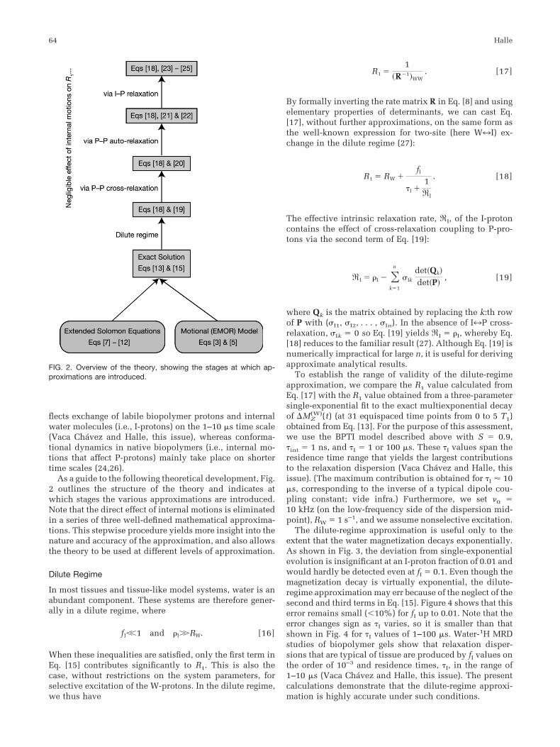
flects exchange of labile biopolymer protons and internalwater molecules (i.e., I-protons) on the 1–10 �s time scale(Vaca Chavez and Halle, this issue), whereas conforma-tional dynamics in native biopolymers (i.e., internal mo-tions that affect P-protons) mainly take place on shortertime scales (24,26).

As a guide to the following theoretical development, Fig.2 outlines the structure of the theory and indicates atwhich stages the various approximations are introduced.Note that the direct effect of internal motions is eliminatedin a series of three well-defined mathematical approxima-tions. This stepwise procedure yields more insight into thenature and accuracy of the approximation, and also allowsthe theory to be used at different levels of approximation.

Dilute Regime

In most tissues and tissue-like model systems, water is anabundant component. These systems are therefore gener-ally in a dilute regime, where

fI��1 and �I��RW. [16]

When these inequalities are satisfied, only the first term inEq. [15] contributes significantly to R1. This is also thecase, without restrictions on the system parameters, forselective excitation of the W-protons. In the dilute regime,we thus have

R1 �1

�R 1WW. [17]

By formally inverting the rate matrix R in Eq. [8] and usingelementary properties of determinants, we can cast Eq.[17], without further approximations, on the same form asthe well-known expression for two-site (here W7I) ex-change in the dilute regime (27):

R1 � RW �fI

�I �1�I

. [18]

The effective intrinsic relaxation rate, �I, of the I-protoncontains the effect of cross-relaxation coupling to P-pro-tons via the second term of Eq. [19]:

�I � �I � �k�1

n

�Ik

det�Qk

det�P, [19]

where Qk is the matrix obtained by replacing the k:th rowof P with (�I1, �I2, . . . , �In). In the absence of I7P cross-relaxation, �Ik � 0 so Eq. [19] yields �I � �I, whereby Eq.[18] reduces to the familiar result (27). Although Eq. [19] isnumerically impractical for large n, it is useful for derivingapproximate analytical results.

To establish the range of validity of the dilute-regimeapproximation, we compare the R1 value calculated fromEq. [17] with the R1 value obtained from a three-parametersingle-exponential fit to the exact multiexponential decayof �MZ

(W)(t) (at 31 equispaced time points from 0 to 5 T1)obtained from Eq. [13]. For the purpose of this assessment,we use the BPTI model described above with S � 0.9,�int � 1 ns, and �I � 1 or 100 �s. These �I values span theresidence time range that yields the largest contributionsto the relaxation dispersion (Vaca Chavez and Halle, thisissue). (The maximum contribution is obtained for �I � 10�s, corresponding to the inverse of a typical dipole cou-pling constant; vide infra.) Furthermore, we set �0 �10 kHz (on the low-frequency side of the dispersion mid-point), RW � 1 s–1, and we assume nonselective excitation.

The dilute-regime approximation is useful only to theextent that the water magnetization decays exponentially.As shown in Fig. 3, the deviation from single-exponentialevolution is insignificant at an I-proton fraction of 0.01 andwould hardly be detected even at fI � 0.1. Even though themagnetization decay is virtually exponential, the dilute-regime approximation may err because of the neglect of thesecond and third terms in Eq. [15]. Figure 4 shows that thiserror remains small (�10%) for fI up to 0.01. Note that theerror changes sign as �I varies, so it is smaller than thatshown in Fig. 4 for �I values of 1–100 �s. Water-1H MRDstudies of biopolymer gels show that relaxation disper-sions that are typical of tissue are produced by fI values onthe order of 10–3 and residence times, �I, in the range of1–10 �s (Vaca Chavez and Halle, this issue). The presentcalculations demonstrate that the dilute-regime approxi-mation is highly accurate under such conditions.

FIG. 2. Overview of the theory, showing the stages at which ap-proximations are introduced.

64 Halle

Internal Motions

Although Eq. [17] (or the equivalent Eqs. [18] and [19]) isaccurate, it is inconvenient to use in practice because itinvolves the high-dimensional polymer relaxation matrixP, which, moreover, requires knowledge of all proton-proton separations and internal motions in the polymer.Fortunately, Eq. [19] can be further simplified under typ-ical tissue conditions. We carry out this simplification inthree steps, as described below.

In the first step we neglect all cross-relaxation rates, �kl,between polymer protons. The relaxation matrix P is thendiagonal, so that det(Qk) � (�Ik/�k)det(P) and Eq. [19]reduces to

�I � �k�1

n ��Ik ��Ik

2

�k. [20]

The accuracy of this approximation essentially relies onthe ratios ��kl�/�k being small compared to unity. Fornearly all �kl, this will be the case simply because �kl

involves only a single dipole coupling, whereas �k in-volves n dipole couplings, some of which will be at least asstrong as the one between protons k and l. Moreover,whereas �k is dominated by a few strong dipole couplingsto nearby protons, most of the �kl are negligibly smallbecause of the large separation between most proton pairs.

To assess the accuracy of Eq. [20] quantitatively, weagain use the BPTI model. In Fig. 5 we compare the R1

dispersion profiles computed from either Eq. [17] (solidcurve) or Eqs. [18] and [20] (dashed curve). The difference

is negligibly small at all frequencies for the parametervalues used: S � 0.9, �int � 10 ns, and �I � 10 �s. Theinternal motions that establish the typical order parameterS � 0.9 in freely tumbling proteins have correlation timesshorter than 100 ps, and much slower internal motionsmodulate only a very small fraction of the dipole coupling(24). By using the value �int � 10 ns, we are thus likelyoverestimating the effect of internal motions considerably.The inset in Fig. 5 shows that Eq. [20] underestimates R1

by at most 0.1% and 2.5% at the low-frequency (104 Hz)and high-frequency (105 Hz) ends, respectively, of thedispersion when �int varies from 0.1 ns to 1 �s (for �I �10 �s and S � 0.9). For all eight hydroxyl protons in BPTI(in Ser, Thr, and Tyr side-chains), the corresponding max-imum relative errors fall in the ranges of 0.08–0.15% and2.2–4.3%. In the limits of very fast (�int � 0) or very slow(S � 1) internal motion, where �k � �Ik and �kl � 0according to Eqs. [6] and [10], the matrix P is rigorouslydiagonal so that Eq. [19] becomes identical to Eq. [20].

Equation [20] still contains the autorelaxation rate, �k, ofP-proton k, which involves dipole couplings to the I-pro-ton and to the n–1 other P-protons (see Eq. [10a]). As thesecond simplifying step, we neglect the effect of the latter,i.e., we write �k � �Ik. This approximation is justified ifthe dispersion is dominated by I-proton exchange ratherthan by polymer internal motions, as appears to be the case(Vaca Chavez and Halle, this issue). In view of Eqs. [3] and[6], this condition becomes (1 S2)�int ¥l Dkl

2 �� S2�I DIk2 .

Replacing �k by �Ik in Eq. [20] and using Eq. [11], we obtainafter some algebra:

FIG. 3. Water-1H magnetization decay after nonselective excitation,calculated exactly with Eq. [13] for the BPTI model with I-protonresidence time �I � 1 �s (●) or 100 �s (E). Other parameter values:fI � 0.01, �int � 1 ns, S � 0.9, RW � 1 s–1, and �0 � 10 kHz. Thecurves resulted from three-parameter single-exponential fits. Theinset shows the root-mean-square error in such fits as a function ofthe intermediary proton fraction, fI, for �I � 1 �s or 100 �s, and otherparameter values as in the main figure.

FIG. 4. Water-1H longitudinal relaxation rate, R1, after nonselectiveexcitation vs. I-proton fraction, fI, for the BPTI model with �I �100 �s. R1 was obtained from a single-exponential fit to the exactmagnetization decay computed from Eq. [13] (solid curve), or wascalculated from the dilute-regime approximation, Eq. [17] (dashedcurve). Other parameter values: �int � 1 ns, S � 0.9, RW � 1 s–1, and�0 � 10 kHz. The inset shows the relative difference (in %) betweenthe two R1 values for �I � 1 �s or 100 �s, with the same abscissa(fI) and parameter values as in the main figure.

Theory of Tissue-Water Relaxation 65

�I � �k�1

n 320.2J�Ik��0 � 0.8J�Ik�2�0� H�Ik��0, [21]

with

H�Ik��0 �2J�Ik�0 � 3J�Ik��0

J�Ik�0 � 3J�Ik��0 � 6J�Ik�2�0. [22]

Except for the factor H(Ik)(�0), which increases monoton-ically with �0 from 1/2 to 2, each term in Eq. [21] is of theform expected for dipolar relaxation of a pair of “like-spin”protons (13). This important feature is a result of I7kcross-relaxation and it means that �I will approach zero athigh frequencies, that is, there will not be a high-frequencyplateau associated with the adiabatic spectral densityJ(Ik)(0).

The spectral density function in Eq. [5b], which appearsin Eqs. [21] and [22], has contributions from exchange aswell as from internal motion of the I–k vector. While suchinternal motions may play a role, e.g., for the labile protonsin a flexible lysine side-chain, we shall, as the third sim-plifying step, ignore their effect on the assumption that (1 S2)�int �� S2�I (as already assumed for the k–l vectors).The spectral density is then given by Eq. [3], and Eq. [21]reduces to the simple form:

�I �32�DIPSIP

2HI��0� 0.2�I

1 � ��0�I2 �

0.8�I

1 � �2�0�I2�, [23]

with

HI��0 �5 � 22��0�I

2 � 8��0�I4

10 � 23��0�I2 � 4��0�I

4 , [24]

and

DIPSIP ��0

4��2���

k�1

n SIk2

rIk6 1/2

. [25]

In Fig. 5 we compare R1 computed from Eqs. [18] and[23]–[25] (dash-dotted curves) with the “exact” R1 ob-tained with Eq. [17]. As anticipated, the approximation isvalid if the internal motions are much faster than theexchange. If this is not the case, an internal motion dis-persion appears in addition to the exchange dispersion, asshown in Fig. 5. In practice, a modest internal motioncontribution is not likely to be resolved in an extendeddispersion profile resulting from several exchange contri-butions with different residence times. For the largest �int

values in Fig. 5, about half of the error associated with Eq.[23] comes from the neglect of internal motion of the I–kvectors.

It can be shown from Eq. [19] that �I � �I, so the effectof I7P cross-relaxation is always to reduce the intrinsicrelaxation rate, �I, of the I-proton below its auto-relaxationrate, �I. In the absence of internal-motion effects (meaningeither very fast or very slow internal motion; vide supra),the P-protons do not cross-relax with each other (�kl � 0)so the relaxation rate of the I-proton becomes a sum of nindependent contributions from isolated “like-spin” pairs(with the dominant contribution from adjacent P-protons).Figure 6 illustrates the effect of cross-relaxation at differ-ent frequencies. At low frequencies (�0�I �� 1), we have �I

FIG. 5. Water-1H relaxation dispersion, R1(�0), for the BPTI model.R1 was calculated from the “exact” Eq. [17] (solid curve), from thediagonal approximation in Eq. [20] (dashed curve) or from the pure-exchange approximation in Eqs. [23]–[25] (dash-dotted curve). Pa-rameter values: fI � 0.001, �I � 10 �s, �int � 10 ns, S � 0.9, andRW � 1 s–1. The inset shows the error, (R1

exact R1approx)/R1

exact, inpercent for the diagonal (dashed curves) and pure exchange (dash-dotted curves) approximations as a function of the internal-motioncorrelation time, �int. The other parameters have the same values asin the main figure, and the frequency, �0, is either 10 or 100 kHz.

FIG. 6. Autorelaxation rate, �I, and effective intrinsic relaxation rate,�I, for the BPTI model. �I was obtained from the “exact” Eq. [17]with �int � 0 (solid curve) or �int � 10 ns (dashed-dotted curve). Theother parameter values are the same as in Fig. 5.

66 Halle

� (1/ 2) ¥k (�Ik � �Ik) � (3/4)�I. At the frequency �0 ��5/(2�I), the cross-relaxation rates, �Ik, vanish so that �I ��I (this only happens for a model with a single residencetime, �I). At high frequencies (�0�I �� 1), we have �I � 2¥k (�Ik � �Ik). This is �� �I, since the adiabatic spectraldensity, J(Ik)(0), cancels out in the sum �Ik � �Ik. In thepresence of internal motions, this cancellation is not per-fect, and both �I (Fig. 6) and R1 (Fig. 5) exhibit an addi-tional dispersion at frequencies where �0�int � 1.

The preceding results are applicable to both internalwater molecules and labile protons. For an internal watermolecule we use Eq. [12] in place of Eq. [11], and the finalresult for the effective intrinsic relaxation rate, �I, of thetwo water protons comprising class I differs from Eq. [23]only through the substitution:

�DIPSIP2HI��0 3 �DWSW

2 � �DWPSWP2HI��0, [26]

where DW and SW are the dipole coupling constant andorder parameter for the intramolecular water H–H vector,respectively, and

DWPSWP ��0

4��2��1

2 �k�1

n �Sak2

rak6 �

Sbk2

rbk6 �1/2

. [27]

As long as the dilute-regime inequalities [16] are satisfied,the theory is readily generalized to the case in which classI contains an arbitrary number of different labile protonsand/or internal water molecules. In Eq. [18] we then sim-ply sum over the different species that make up the inter-mediary (I) proton class:

R1 � RW � �n

fI,n

�I,n �1

�I,n

. [28]

Adiabatic Regime

In the fast-exchange regime, where �I�I �� 1, Eqs. [18] and[23] yield

R1 � RW �32

fI�DIPSIP2HI��0� 0.2�I

1 � ��0�I2 �

0.8�I

1 � �2�0�I2�.

[29]

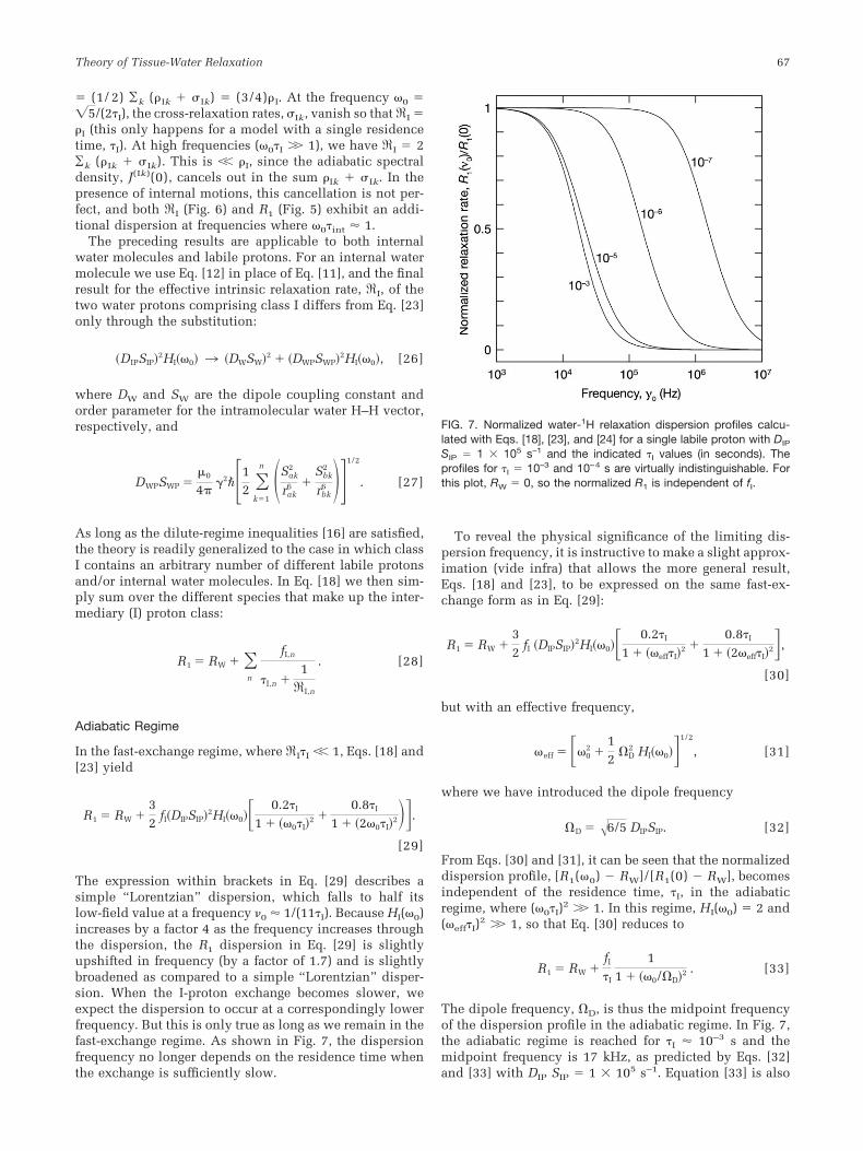
The expression within brackets in Eq. [29] describes asimple “Lorentzian” dispersion, which falls to half itslow-field value at a frequency �0 � 1/(11�I). Because HI(�0)increases by a factor 4 as the frequency increases throughthe dispersion, the R1 dispersion in Eq. [29] is slightlyupshifted in frequency (by a factor of 1.7) and is slightlybroadened as compared to a simple “Lorentzian” disper-sion. When the I-proton exchange becomes slower, weexpect the dispersion to occur at a correspondingly lowerfrequency. But this is only true as long as we remain in thefast-exchange regime. As shown in Fig. 7, the dispersionfrequency no longer depends on the residence time whenthe exchange is sufficiently slow.

To reveal the physical significance of the limiting dis-persion frequency, it is instructive to make a slight approx-imation (vide infra) that allows the more general result,Eqs. [18] and [23], to be expressed on the same fast-ex-change form as in Eq. [29]:

R1 � RW �32

fI �DIPSIP2HI��0� 0.2�I

1 � ��eff�I2 �

0.8�I

1 � �2�eff�I2�,

[30]

but with an effective frequency,

�eff � ��02 �

12�D

2 HI��0�1/2

, [31]

where we have introduced the dipole frequency

�D � 6/5 DIPSIP. [32]

From Eqs. [30] and [31], it can be seen that the normalizeddispersion profile, [R1(�0) RW]/[R1(0) RW], becomesindependent of the residence time, �I, in the adiabaticregime, where (�0�I)

2 �� 1. In this regime, HI(�0) � 2 and(�eff�I)

2 �� 1, so that Eq. [30] reduces to

R1 � RW �fI

�I

11 � ��0/�D

2 . [33]

The dipole frequency, �D, is thus the midpoint frequencyof the dispersion profile in the adiabatic regime. In Fig. 7,the adiabatic regime is reached for �I � 10–3 s and themidpoint frequency is 17 kHz, as predicted by Eqs. [32]and [33] with DIP SIP � 1 � 105 s–1. Equation [33] is also

FIG. 7. Normalized water-1H relaxation dispersion profiles calcu-lated with Eqs. [18], [23], and [24] for a single labile proton with DIP

SIP � 1 � 105 s–1 and the indicated �I values (in seconds). Theprofiles for �I � 10–3 and 10–4 s are virtually indistinguishable. Forthis plot, RW � 0, so the normalized R1 is independent of fI.

Theory of Tissue-Water Relaxation 67

valid for an internal water molecule in the adiabatic re-gime, but then the dipole frequency is (see Eq. [26])

�D � �35�DWSW

2 � 2�DWPSWP2��1/2

. [34]

Whereas the dispersion frequency is independent of �I inthe adiabatic regime, the dispersion amplitude, or R1(0) –RW, is inversely proportional to �I (see Eq. [33]). Thiscontrasts with the extreme-narrowing limit, where the dis-persion amplitude is proportional to �I (see Eq. [29] with�0�I �� 1). The dispersion amplitude must therefore ex-hibit a maximum as a function of �I, as shown in Fig. 8.According to Eqs. [18] and [23], this maximum occurs for�I � �8/5/�D. It can also be seen in Fig. 8 that Eqs. [30]and [31] differ very little from the more accurate result inEqs. [18] and [23]–[25]. The difference is largest (about10%) for �0 � 0 and �I � 1/�D. Both results reduce to Eq.[33] in the adiabatic regime.

In the past, adiabatic dispersion profiles have often beenanalyzed with fast-exchange theories. This has led to themistaken belief that the motional correlation time (de-duced from the dispersion midpoint) is invariant withrespect to system properties and temperature (2,4,5). Infact, the apparent correlation time obtained in this way isnot related to molecular motions. It is simply the inverse ofthe dipole frequency �D, which indeed is expected toexhibit these invariances. For example, for the leftmostdispersion profile in Fig. 7, the apparent correlation time is13 �s, whereas the true correlation time is two orders ofmagnitude longer (1 ms).

Beyond the Motional-Narrowing Regime

The preceding implementation of the EMOR model isbased on the extended Solomon equations with the usual

expressions for auto-relaxation and cross-relaxation rates(12,13). These expressions are valid only in the motional-narrowing regime, which for R1 and in our notation isdefined by the inequality (�D�I)

2 �� 1 � (�0�I)2. At first

sight, this condition appears to restrict the applicability ofthe present theory considerably. In particular, the validityof the results shown in the right half of Fig. 8 may bequestioned. Fortunately, it turns out that the present the-ory remains valid outside the motional-narrowing regime,as explained below.

In essence, the problem is this: when the residence (orexchange) time is also the correlation time that drives spinrelaxation, the motional-narrowing condition will be vio-lated as soon as the system leaves the fast-exchange re-gime. In other words, fast exchange and motional narrow-ing are synonymous. However, we are concerned here onlywith the dilute regime, fI �� 1, where any given protonspends only a small fraction of the time in an I-site. Thestochastically modulated, residual dipole coupling thatinduces relaxation is thus a sparse coupling: it is essen-tially zero for long periods of time (on average �I /fI) andonly intermittently assumes large values (of order 105 s–1)for brief periods (on average �I). The present theory istherefore valid without restrictions on the dimensionlessparameters �0�I and �D�I, as long as the system is in thedilute regime.

To justify this claim, let us consider an isolated two-spinsystem, such as a water molecule exchanging between W-and I-sites. This is like the EMOR model, except that thereare no P-protons to couple with the I-protons. For thissimpler version of the EMOR model, the exact solution hasbeen obtained from an analytical solution of the stochasticLiouville equation (Halle and Nilsson, unpublished re-sults). The exact result is somewhat lengthy, but it deviatesonly slightly (and then only when both �0�I and �D�I arelarge) from the simple expression:

R1 � RW �32

fI �DWWSWW2� 0.2�I

1 � ���D�I2 � ��0�I

2

�0.8�I

1 � ���D�I2 � �2�0�I

2�, [35]

where the dipole frequency is now defined as ��D � (3/2) DWWSWW. This result should be compared with Eq. [30]with HI(�0) � 1 (since there are no P-protons) and DIP SIP

3 DWW SWW. For this comparison we make use of thehighly accurate approximation: 0.2/(1�x) � 0.8/(1�4x) �1/(1�3x). We thus find that the two results coincide, ex-cept for a 10% difference in the dipole frequency appear-ing in the numerator of the dispersive terms.

Spin Diffusion

Whereas all dipole couplings involving I-protons are mo-tionally averaged (to zero if the system is isotropic) byexchange, dipole couplings between two P-protons areeither static or contain a dominant static part that remainsafter partial averaging by restricted internal motions.These static dipole couplings give rise to a coherent spinevolution that we have ignored so far.

FIG. 8. Low-field water-1H relaxation rate, R1(0), for a single labileproton with DIP SIP � 1 � 105 s–1 and fI � 10–3 as a function of thelabile-proton residence time, �I. For this plot, RW � 0. R1 wascalculated with Eqs. [18], [23], and [24] (solid curve) or with Eqs. [30]and [31] (dashed curve).

68 Halle

We assume that the external magnetic field is muchstronger than the local dipolar field: �0 �� Dkl, corre-sponding to Larmor frequencies, �0, higher than 1–10 kHz.At lower fields, the Zeeman energy is no longer conservedand spin angular momentum exchanges with the collec-tive orbital angular momentum of the lattice (28). In thehigh-field regime, the nonsecular part of the static dipolarspin Hamiltonian can be neglected, whereas the secularI�(k)I�

(l ) terms induce energy-conserving mutual spin flips inprotons k and l (13). In a macroscopic sample the net resultof these spin flips is to reduce any differences in longitu-dinal magnetization among the protons according to (29)

dMZ�k

dt� �

l�1l�k

n

Wkl �MZ�l � MZ

�k, [36]

where Wkl is the probability per unit time that protons kand l undergo a mutual spin flip. For spins on a homoge-neous lattice, Eq. [36] leads, in the continuum limit, to adiffusion equation that describes the homogenization of aninitially nonuniform magnetization (29,30). In our nota-tion the spin-flip rate is given by

Wkl ��20

SklDkl. [37]

A comparison of Eqs. [7] and [36] shows that spin diffu-sion can be taken into account approximately, at least for�0 �� Dkl, by making the following substitutions in therelaxation matrix P in Eq. [9]:

�k 3 �k � �l�1l�k

n

Wkl, [38a]

�kl 3 �kl � Wkl. [38b]

Note that we only include spin diffusion among P-protons.The coherent evolution of proton pairs I–k will bequenched by the exchange if the I-proton residence time,�I, is much shorter than the spin-flip time, 1/WIk. FromEqs. [4] and [37] we estimate the shortest possible spin-fliptime to 0.3 ms, corresponding to a proton-proton separa-tion of 2.2 Å (the smallest value for the hydroxyl protonsin BPTI) and a plausible side-chain order parameter of 0.6.As shown in Fig. 8, the relaxation dispersion is dominatedby I-protons with residence times that are much shorterthan the shortest spin-flip time of 0.3 ms. We thereforeconclude that spin diffusion between I- and P-protonsplays an insignificant, if not negligible, role.

Figure 9 shows how spin diffusion among P-protons,modeled with the aid of Eqs. [37] and [38], affects thedispersion profile. The thick dashed curve corresponds tothe solid curve in Fig. 5 with �I � 10 �s and �int � 10 ns(and no spin diffusion). The main effect of spin diffusion isto enhance the amplitude of the high-frequency internal-motion dispersion step (thin dashed curve). The observeddispersion profile is dominated by exchange-modulateddipole couplings between the I-proton (I) and nearby P-

protons. In the absence of spin diffusion, cross-relaxationlargely cancels the adiabatic J(Ik)(0) contribution to �I (seeEq. [11]), thereby making �I �� �I in the high-frequencyrange (Fig. 9, inset). In the presence of spin diffusionamong P-protons, the relaxation of the I-proton can nolonger be (approximately) attributed to independent “like-spin” I–k pairs, and the effect of I–k cross-relaxation islargely quenched. Because the adiabatic contribution isnot canceled, �I now becomes comparable to �I (Fig. 9,inset).

The effect of spin diffusion on the water-1H dispersiondecreases as the internal motion becomes faster. This isillustrated in Fig. 9 for �int � 1 ns (solid curves). In fact,spin diffusion among P-protons has no effect at all on thewater-1H integral relaxation rate R1 if the internal motionsthat modulate the P–P and I–P dipole couplings are eithervery fast (�int � 0, effectively) or very slow (S � 1, effec-tively). This rigorous result, which is also valid outside thedilute regime, follows from Eqs. [3], [5], [6], [8]–[11], [15],and [38]. Seen in the light of our theoretical analysis, theabsence of a pronounced high-frequency step in water-1Hdispersion profiles from tissue (1,2) and biopolymer gels(Vaca Chavez and Halle, this issue) indicates that the ef-fects of internal motions and spin diffusion are unimpor-tant.

Although spin diffusion appears to be unimportant forwater-1H relaxation in tissue and gels, it does effect theevolution of the P-proton magnetization. For P-protons,the exchanging I-protons are likely to act as a more effi-cient relaxation sink than the rotating methyl groups thatusually drive spin diffusion in solid polymers (29).

FIG. 9. Water-1H relaxation dispersion, R1(�0), for the BPTI model.R1 was calculated from the “exact” Eq. [17] with �int � 1 ns (solidcurves) or 10 ns (dashed curves). Other parameter values are as inFigs. 5 and 6, and without (thick curves) or with (thin curves) spindiffusion among all P-protons according to Eqs. [37] and [38]. Theinset shows the effective intrinsic relaxation rate, �I (solid curves),and the auto-relaxation rate, �I (dashed curve), without (thick curve)or with (thin curve) spin diffusion, in all cases for �int � 10 ns.

Theory of Tissue-Water Relaxation 69

DISCUSSION

Other Models

Most previous theories of water-1H relaxation in tissuewere based on a phenomenological description of magne-tization exchange between two bulk proton phases (20,25).In this so-called two-pool model, water (W) and polymer(P) phases, with intrinsic longitudinal relaxation rates rW

and rP, exchange magnetization at rates rW3P and rP3W:

¢OrW

W-|0rW3P

rP3W

P ¡rP

. [39]

This scheme assumes (among other things) fast exchangebetween intermediary protons and external water so thatthese classes (denoted by I and W in the EMOR model) canbe treated as a single homogenous proton phase (denotedby W in the two-pool model). In the absence of internalmotions and in the dilute regime (fI �� 1), the two-poolmodel makes essentially the same prediction as the EMORmodel does in the fast-exchange regime. However, the twomodels differ qualitatively outside the fast-exchange re-gime.

Previous water-1H and 2H MRD studies of chemicallycross-linked protein gels revealed a remarkable invarianceof the dispersion frequency with respect to temperatureand biopolymer (2,4,5). The authors interpreted that find-ing in terms of the two-pool model by postulating theexistence, in all investigated proteins, of a class of watermolecules with a long (1 �s), but temperature-indepen-dent, residence time (2,4,5). Such unphysical assumptionsare not required by the EMOR model, which predicts aninvariant dispersion frequency that is equal to the residualdipole frequency �D, in the adiabatic regime. We previ-ously presented this argument in connection with 2H MRDprofiles (31,32), and Eq. [33] and Fig. 7 show that it holdsalso for the 1H MRD profile.

Several authors have argued that water-1H dispersionsin tissue and biopolymer gels are produced by collectivepolymer vibration modes (7–10). The frequency depen-dence is thus taken to enter via the intrinsic relaxationrate, rP, of the P-proton pool. This view contrasts sharplywith the EMOR model, which effectively sets rP � 0. Acritical assumption in these models is that the vibrationalmodes evolve in a space of reduced dimensionality, lead-ing to a power-law decay, rP(�0) � A�0

p, with p � 1.Except at the highest experimental frequencies, these mod-els predict that rP �� rW, in which case the two-poolmodel yields

R1 �xPrPk

�rP � k2 � 4xPrPk�1/2 , [40]

where k � rW3P � rP3W is the magnetization exchangerate constant, and xW and xP are the equilibrium protonfractions in the two pools. At low frequencies the limit ofslow magnetization transfer, k �� rP, is reached, where Eq.[40] reduces to R1 � xPk � rW3P. At higher frequencies(typically � 105 Hz), where magnetization transfer is fast,Eq. [40] yields R1 � xPrP, so the observed R1 dispersion isa scaled replica of the rP dispersion.

According to the most recent version of the collectivevibration model, P-proton relaxation is induced by local-ized vibration modes (fractons) in a percolation cluster(8–10). To account for the observed dispersion profile, thisfracton model requires that the vibrational density of statesscales (anomalously) as �1/3 from 104 to 108 Hz. However,both experiment (33) and theory (34) support a classic �2

scaling up to �1012 Hz. Apart from its questionable phys-ical basis, the fracton/two-pool model cannot explain thestrong pH dependence seen in water-1H dispersion pro-files from gelatin gels (Vaca Chavez and Halle, this issue)even at frequencies above �100 kHz, where the observedR1 dispersion is predicted to be a scaled replica of rP (videsupra). In the EMOR model this observation is readilyexplained by the acid- and base-catalyzed labile-protonexchange (Vaca Chavez and Halle, this issue). The fracton/two-pool theory also cannot explain the R1 maximum ob-served as a function of temperature for agarose gels (11,35). At frequencies above �100 kHz, this theory predictsthat R1 � rP � T. On the low-frequency plateau, whereR1 � rW3P, the identification (10) rW3P � fI /(T2,solid � �I)with T2,solid � 10 �s taken to be governed by temperature-independent spin diffusion (10), it is clear that R1 cannotdecrease with temperature. In contrast, the EMOR modelaccounts quantitatively for the R1 maximum in terms ofthe temperature-dependent residence time of internal wa-ter molecules (11).

From Model System to Tissue

In the companion paper to this study (Vaca Chavez andHalle, this issue), we show that the EMOR model, withphysically reasonable parameter values, can account for anextensive set of water-1H MRD data from aqueous agaroseand gelatin gels. In the following, we argue that the EMORmodel also provides a basis for the analysis and predictionof MRD profiles from tissue, and thus allows T1 contrast tobe exploited more rationally in clinical MRI investiga-tions.

Although tissues are structurally and chemically morecomplex than biopolymer gels, they contain rotationallyimmobile proteins and other macromolecules with thesame types of intermediary proton as in the gels. A roughestimate indicates that most types of soft tissue are in thedilute regime (fI �� 1), as assumed in the theory. From theknown (36) frequency of occurrence in proteins of aminoacids carrying labile protons (Asp, Glu, Ser, Thr, Tyr, His,Lys, and Arg) and from the observation that proteins con-tain on average one internal water molecule per 27 aminoacid residues (37), the fraction of intermediary protons canbe estimated as

fI � f IP � f I

W � �5.2 � 10 2 � 5.6 � 10 3mP

mW[41]

where f IP refers to labile protons in protein side-chains,

and f Iw refers to protons in internal water molecules. Fur-

ther, mP and mW are the masses (or mass fractions) ofprotein and water, respectively, in the tissue. For skeletalmuscle, with mP � 0.20 and mW � 0.75 (38), Eq. [41] yieldsfI � 1.5 � 10–2, so this tissue type is in the dilute regime.This is also the case for nerve and vascular tissues, which

70 Halle

contain even more water (38). On the other hand, epithe-lial and connective tissues may not be in the dilute regime.It should be noted that Eq. [41] overestimates fI for tworeasons. First, at any given pH, only some of the eighttypes of labile proton will contribute to the water-1H dis-persion (Vaca Chavez and Halle, this issue). Second, onlylabile protons and internal water molecules in immobileproteins contribute (vide supra).

Any tissue contains labile protons and internal watermolecules with a wide range of residence times, but all ofthese protons have dipole coupling constants on the orderof 105 s–1. According to the EMOR model, the observed R1

dispersion should then be dominated by intermediary pro-tons with residence times near 10–5 s (see Fig. 8). Thenormalized dispersion profile should therefore be similarto the �I � 10–5 s curve in Fig. 7, but broadened on thehigh-frequency side due to I-protons with shorter resi-dence times. This is indeed what is observed in mosttissues (1,2). Typically the dispersion is only measureddown to 10 kHz, where the approach to the low-frequencyR1 plateau is just barely apparent (see the �I � 10–5 s curvein Fig. 7). This experimental limitation has made the in-terpretation of water-1H MRD profiles particularly chal-lenging.

The molecular theory presented here provides a quanti-tative basis for 1H MRD investigations of structure anddynamics in tissues and other aqueous systems with im-mobile (or slowly tumbling) biopolymers. Even though thewater-1H dispersion occurs in the mT magnetic-fieldrange, the present work has at least two bearings on clin-ical MRI applications. First, the strong field dependence ofT1 in the mT range is a potential source of tissue contrast,as demonstrated in a recent MRI study with pulsed prepo-larization and detection by a superconducting quantuminterference device (39). Second, even at the 1.5–3.0 Tfields typically used in MRI, the EMOR model can beapplied to the zero-frequency dipolar contributions totransverse relaxation and to selective magnetization trans-fer and to the low-frequency dipolar contribution to rotat-ing-frame spin-lattice relaxation.

CONCLUSIONS

In this work we have presented a molecular theory forwater-1H spin-lattice relaxation in tissue and other aque-ous systems with rotationally immobile macromolecules.The theory is based on the EMOR model, according towhich spin relaxation is induced by exchange-mediatedorientational randomization of labile biopolymer protonsor internal water molecules. These intermediary protonscouple bulk-water and biopolymer protons via dipolarcross-relaxation and material exchange.

Unlike the phenomenological two-pool model, whichimplicitly assumes fast exchange, the EMOR model is de-veloped from a truly molecular perspective. By applyingthe rigorous principles of nuclear spin relaxation and in-troducing well-defined approximations, we obtained asimple analytical expression for R1 that is quantitativelyvalid over the relevant range of system parameters. Theapproximations were tested against exact numerical calcu-lations for a realistic model system and found to be validunder conditions typical of water-rich tissue and biopoly-

mer gels. We have also presented arguments against coher-ent spin diffusion and collective biopolymer vibrations assignificant determinants of the water-1H relaxation disper-sion.

REFERENCES

1. Bryant RG, Mendelson DA, Lester CC. The magnetic field dependenceof proton spin relaxation in tissues. Magn Reson Med 1991;21:117–126.

2. Koenig SH, Brown RD. Relaxometry of tissue. In: Grant D, Harris RK,editors. Encyclopedia of magnetic resonance. New York: Wiley; 1996. p4108–4120.

3. Bottomley PA, Foster TH, Argersinger RE, Pfeifer LM. A review ofnormal tissue hydrogen NMR relaxation times and relaxation mecha-nisms from 1–100 MHz: dependence on tissue type, NMR frequency,temperature, species, excision, and age. Med Phys 1984;11:425–448.

4. Koenig SH, Brown RD. A molecular theory of relaxation and magneti-zation transfer: application to cross-linked BSA, a model for tissue.Magn Reson Med 1993;30:685–695.

5. Koenig SH, Brown RD, Ugolini R. A unified view of relaxation inprotein solutions and tissue, including hydration and magnetizationtransfer. Magn Reson Med 1993;29:77–83.

6. Kimmich R, Nusser W, Gneiting T. Molecular theory for nuclear mag-netic relaxation in protein solutions and tissue: surface diffusion andfree-volume analogy. Colloids Surf 1990;45:283–302.

7. Rorschach HE, Hazlewood CF. Protein dynamics and the NMR relax-ation time T1 of water in biological systems. J Magn Reson 1986;70:79–88.

8. Blinc R, Rutar V, Zupancic I, Zidansek A, Lahajnar G, Slak J. ProtonNMR relaxation of adsorbed water in gelatin and collagen. Appl MagnReson 1995;9:193–216.

9. Korb JP, Bryant RG. The physical basis for the magnetic field depen-dence of proton spin-lattice relaxation rates in proteins. J Chem Phys2001;115:10964–10974.

10. Korb JP, Bryant RG. Magnetic field dependence of proton spin-latticerelaxation times. Magn Reson Med 2002;48:21–26.

11. Vaca Chavez F, Persson E, Halle B. Internal water molecules andmagnetic relaxation in agarose gels. J Am Chem Soc 2006;128:4902–4910.

12. Solomon I. Relaxation processes in a system of two spins. Phys Rev1955;99:559–565.

13. Abragam A. The principles of nuclear magnetism. Oxford: ClarendonPress; 1961.

14. Halle B. Protein hydration dynamics in solution: a critical survey. PhilTrans R Soc Lond B 2004;359:1207–1224.

15. Modig K, Liepinsh E, Otting G, Halle B. Dynamics of protein andpeptide hydration. J Am Chem Soc 2004;126:102–114.

16. Halle B. Water in biological systems: the NMR picture. In: Bellisent-Funel MC, editor. Hydration processes in biology. Dordrecht: IOSPress; 1998. p 233–249.

17. Denisov VP, Halle B. Hydrogen exchange rates in proteins from water1H transverse magnetic relaxation. J Am Chem Soc 2002;124:10264–10265.

18. Venu K, Denisov VP, Halle B. Water 1H magnetic relaxation dispersionin protein solutions. A quantitative assessment of internal hydration,proton exchange, and cross-relaxation. J Am Chem Soc 1997;119:3122–3134.

19. Halle B, Denisov VP, Venu K. Multinuclear relaxation dispersion stud-ies of protein hydration. In: Krishna NR, Berliner LJ, editors. Biologicalmagnetic resonance. Vol. 17. New York: Kluwer Academic/PlenumPress; 1999. p 419–484.

20. Edzes HT, Samulski ET. The measurement of cross-relaxation effects inthe proton NMR spin-lattice relaxation of water in biological systems:hydrated collagen and muscle. J Magn Reson 1978;31:207–229.

21. van Kampen NG. Stochastic processes in physics and chemistry.Amsterdam: North-Holland; 1981.

22. Dattagupta S. Relaxation phenomena in condensed matter physics.London: Academic Press; 1987.

23. Wlodawer A, Walter J, Huber R, Sjolin L. Structure of bovine pancreatictrypsin inhibitor. Results from joint neutron and x-ray refinement ofcrystal form II. J Mol Biol 1984;180:301–329.

24. Palmer AG. NMR probes of molecular dynamics: overview and com-parison with other techniques. Annu Rev Biophys Biomol Struct 2001;30:129–155.

Theory of Tissue-Water Relaxation 71

25. Zimmerman JR, Brittin WE. Nuclear magnetic resonance studies inmultiple phase systems: lifetime of a water molecule in an adsorbingphase on silica gel. J Phys Chem 1957;61:1328–1333.

26. McCammon JA, Harvey SC. Dynamics of proteins and nucleic acids.Cambridge: Cambridge University Press; 1987.

27. Torrey HC, Korringa J, Seevers DO, Uebersfeld J. Magnetic spin pumpingin fluids contained in porous media. Phys Rev Lett 1959;3:418–419.

28. Sodickson DK, Waugh JS. Spin diffusion on a lattice: classical simula-tions and spin coherent states. Phys Rev B 1995;52:6467–6479.

29. Cheung TTP. Spin diffusion in solids. In: Grant D, Harris RK, editors.Encyclopedia of magnetic resonance. New York: Wiley; 1996. p 4518–4524.

30. Cheung TTP. Spin diffusion in NMR in solids. Phys Rev B 1981;23:1404–1418.

31. Halle B. Spin dynamics of exchanging quadrupolar nuclei in locallyanisotropic systems. Progr NMR Spectrosc 1996;28:137–159.

32. Halle B, Denisov VP. A new view of water dynamics in immobilizedproteins. Biophys J 1995;69:242–249.

33. Lushnikov SG, Svanidze AV, Sashin IL. Vibrational density of states ofhen egg white lysozyme. JETP Lett 2005;82:30–33.

34. Yu X, Leitner DM. Heat flow in proteins: computation of thermaltransport coefficients. J Chem Phys 2005;122:054902.

35. Woessner DE, Snowden BS. Pulsed NMR study of water in agar gels. JColl Interface Sci 1970;34:290–299.

36. Creighton TE. Proteins. 2nd ed. New York: WH Freeman; 1993.37. Williams MA, Goodfellow JM, Thornton JM. Buried waters and internal

cavities in monomeric proteins. Protein Sci 1994;3:1224–1235.38. Harper HA. Review of physiological chemistry. 15th ed. Los Altos, CA:

Lange Medical Publishers; 1973. ch. 22.39. Lee SK, Mo le M, Myers W, Kelso N, Trabesinger AH, Pines A, Clarke

J. SQUID-detected MRI at 132 �T with T1-weighted contrast estab-lished at 10 �T–300 mT. Magn Reson Med 2005;53:9–14.

72 Halle