molecular dynamics study of novel cryoprotectants and … · molecular dynamics study of novel...
TRANSCRIPT

Molecular dynamics study of novel cryoprotectants and of CO2 capture by sI clathrate
hydrates
Michael Nohra
Thesis submitted to the
Faculty of Graduate and Postdoctoral Studies
In partial fulfillment of the requirements
For the MSc degree in Chemistry
Department of Chemistry
Faculty of Science
University of Ottawa
© Michael Nohra, Ottawa, Canada, 2012

ii
Table of Contents
Table of Contents……………………………………………………………………………..ii
Abstract………………………………………………………………………………………iii
List of Figures………………………………………………………………………………..iv
List of Tables………………………………………………………………………………...vi
List of Equations………………………………………………………………………….…vii
List of Abbreviations……………………………………………………………………...…ix
Acknowledgements………………………………………………………………………..….x
Chapter 1: Introduction and applications of molecular dynamics simulations
General introduction………………...……………………………………………..…1
Chapter 2: Investigating ice recrystallization inhibition activity of novel cryprotectants
Introduction…………………………………………………………………………...7
Methodology…………………………………………………………………………21
Computational details…………...…………………………………………………..27
Results and discussion……………………………………………………………….32
Conclusion…………………………………………………………………………...40
Chapter 3: Investigating the feasibility of sI clathrate hydrates as carbon capture tools
Introduction.…………………………………………………………………………46
Methodology.…………………………………………………………...……………58
Computational details.……...…………………………………………………….…70
Results and discussion……………………………………………………………….77
Conclusion.…………………………………………………………..………………94
Chapter 4: Future investigations and applications
Conclusions and future work……………………………………………………….102

iii
Abstract
The first project in this work used classical molecular dynamics to study the ice
recrystallization inhibition potential of a series of carbohydrates and alcochols, using the hydration
index, partial molar volumes and isothermal compressibilities as parameters for measuring their
cryogenic efficacy. Unfortunately, after 8 months of testing, this work demonstrates that the accuracy
and precision of the density extracted from simulations is not sufficient in providing accurate partial
molar volumes. As a result, this work clearly demonstrates that current classical molecular dynamics
technology cannot probe the volumetric properties of interest with sufficient accuracy to aid in the
research and development of novel cryoprotectants.
The second project in this work used molecular dynamics simulations to evaluate the Gibbs
free energy change of substituting CO2 in sI clathrate hydrates by N2,CH4, SO2 and H2S flue gas
impurities under conditions proposed for CO2 capture (273 K, 10 bar). Our results demonstrate that
CO2 substitutions by N2 in the small sI cages were thermodynamically favored. This substitution is
problematic in terms of efficient CO2 capture, since the small cages make up 25% of the sI clathrate
cages, therefore a significant amount of energy could be spent on removing N2 from the flue gas
rather than CO2. The thermodynamics of CO2 substitution by CH4, SO2 and H2S in sI clathrate
hydrates was also examined. The substitution of CO2 by these gases in both the small and large cages
were determined to be favorable. This suggests that these gases may also disrupt the CO2 capture by
sI clathrate hydrates if they are present in large concentrations in the combustion flue stream. Similar
substitution thermodynamics at 200 K and 10 bar were also studied. With one exception, we found
that the substitution free energies do not significantly change and do not alter the sign of
thermodynamics. Thus, using a lower capture temperature does not significantly change the
substitution free energies and their implications for CO2 capture by sI clathrate hydrates.

iv
List of Figures
Figure 1.1: General structure of a naturally occurring AFGPs..……………………………. 2
Figure 1.2: Close-up the small and large cages in
sI clathate hydrate…………………………………………………………..…………………4
Figure 2.1: Structure of native AFGP-8 from Gagus Ogac……………………………….. 11
Figure 2.2: Schematic representation of the quasi-liquid layers…………………………... 13
Figure 2.3: IRI activity of native AFGP-8 and some of its analogues…………………….. 14
Figure 2.4: IRI activity of various monosaccharides and Disaccharides as a
function of the hydration number…………….…………………………………………….. 15
Figure 2.5: IRI activity of various monosaccharides and disaccharides as a
function of the hydration index……………………………………………………...……... 16
Figure 2.6: AFGP-8 analogue; Schematic representation of the hydroxyl
groups participating in hydrogen bonding in a AFGP-8 analogue……………………….… 18
Figure 2.7: Molecular dynamics snapshots of the conformations
for 4 different AFGP analogues...………………………………………………………….. 19
Figure 2.8: Test structures of carbohydrates studied in this work…………………………. 20
Figure 2.9: Isothermal and adiabatic compressibilities behavior of
water at different temperratures………………………………. …………………………....24
Figure 2.10: Snapshot of a simulation cell of a solvated carbohydrate
used in this work……………………………………………………………………………..27
Figure 2.11: Density error analysis for all alcohols……………………………………….. 35
Figure 2.12: Simulated partial molar volume of propanol at
different concentrations…………………………………………………………………….. 36
Figure 2.13: Simulation cell snapshot illustrating propanol interactions
at the MD detection limit…………………………………………………………………… 38
Figure 3.1: SiO2, silicate structure (zeolite)………………………………………..……… 49
Figure 3.2: Clathrate hydrate hydrogen bonding network…………………………………. 50
Figure 3.3: Proposed clathrate hydrate apparatus for CO2 recovery………………………. 51

v
Figure 3.4: Pressure and temperature conditions for hydrate formation…………………... 52
Figure 3.5: Example of carbon dioxide deep sea storage using clathrate hydrates………... 53
Figure 3.6: Ocean floor offering favorable conditions for clathrate formation……………. 53
Figure 3.7: Clathrate hydrate reservoir found under the permafrost………………………. 54
Figure 3.8: The structures of small and large cages in
sI clathrate hydrate…………………………………..……………………………………... 55
Figure 3.9: Snapshot of CO2 → SO2 transformation using
thermodynamic integration in this study……………………………………………….…... 65
Figure 3.10: Free energy behavior
for different λ values
of the CO2→SO2 substitution………………………………………………………………. 72

vi
List of Tables
Table 2.1: Comparison of theoretical and simulated partial molar volumes
for the carbohydrates used in this work…………………………………………………….. 32
Table 2.2: Comparison of theoretical and simulated partial molar volumes
for the alcohols used in this work …………..………………………………….…………... 34
Table 2.3: Partial molar volume of propanol at different simulated concentrations………. 37
Table 3.1: List of atomic point charges and Lennard-Jones parameters
for the molecules used in this work…………………............................................................ 71
Table 3.2: Gibbs free energy of CO2(clathrate) → CH4(clathrate)
substitutions at 273 K and 10 bar………………………………………………………….. 78
Table 3.3: Gibbs free energy of CO2(clathrate) → N2(clathrate)
substitutions at 273 K and 10 bar………………………………………………………..… 81
Table 3.4: Thermophysical data and residual contributions to the
Gibbs free energy for the molecules used in this study…………………………………….. 83
Table 3.5: Simulation cell volumes (Å3) for each clathrate
used in this study………………………………………………….………………………... 84
Table 3.6: Van der Waals radii (Å) and polarity for guest species
used in this work…………………………………………………………….……………… 84
Table 3.7: Gibbs free energy of CO2(clathrate) → SO2(clathrate)
substitutions at 273 K and 10 bar………………………………………………………….. 85
Table 3.8: Gibbs free energy of CO2(clathrate) → H2S(clathrate)
substitutions at 273 K and 10 bar………………………………………………………….. 87
Table 3.9: Gibbs free energy of CO2(clathrate) → Y(clathrate)
substitutions at 200 K and 10 bar………………………………………………………….. 90

vii
List of Equations
Equation 2.1: Hydration index……………………………..……………………………… 21
Equation 2.2: Partial molar volume……………………………………………….………. 21
Equation 2.3: Molality…………………………………………………………………….. 21
Equation 2.4: Hydration number………………………………………………………...... 22
Equation 2.5: Mole fraction……………………………………………………………….. 22
Equation 2.6: Isentropic compressibility………………………………………………….. 23
Equation 2.7: Isentropic-Isothermal compressibility approximation……………….……... 23
Equation 2.8: Isothermal compressibility via fluctuation method………………………… 25
Equation 2.9: Isothermal compressibility via finite difference method…………………… 25
Equation 2.10: Density required in the first simulation
of the finite difference method……………………………………………………………... 26
Equation 2.11: Density required in the second simulation
of the finite difference method…………………………………………………………….. 26
Equation 3.1: Phase 1 reaction of CO2 capture via liquid amine sorbent…………………. 47
Equation 3.2: Phase 2 reaction of CO2 capture via liquid amine sorbent…………………. 47
Equation 3.3: Intra and intermolecular interaction potential energy function…………….. 59
Equation 3.4: Non-bonded potential energy function……………………………………... 59
Equation 3.5: Electrostatic potential………………………………………………………. 59
Equation 3.6: Van der Waals potential……………………………………………………. 60
Equation 3.7: Linear Kirkwood coupling parameter method……………………………... 60
Equation 3.8: Gibbs free energy via thermodynamic integration…………………………. 61
Equation 3.9: Non-linear Kirkwood coupling parameter method…………………………. 62
Equation 3.10: General CO2 sI clathrate substitution reaction with impurity guest Y……. 63
Equation 3.11: CO2 substitution reaction in the clathrate hydrate phase with guest Y….... 63
Equation 3.12: Error function mixing function……………………………………………. 65
Equation 3.13: Polynomial function mixing function……………………………………... 65

viii
Equation 3.14: Trigonometric function mixing function………………………………….. 65
Equation 3.15: Y gas substitution reaction with CO2 in the gas phase………………...….. 66
Equation 3.16: Non-ideality free energy contribution for CO2…………………………………………… 66
Equation 3.17: Residual chemical potential component of the non-ideal contribution..….. 67
Equation 3.18: Total Gibbs free energy for CO2Y guest substitution………..………… 67
Equation 3.19: First ideal gas approximation……………………………………………... 68
Equation 3.20: Second ideal gas approximation…………………………………………... 68
Equation 3.21: Clathrate incompressibility approximation……………………………….. 68
Equation 3.22: Total Gibbs free energy approximation…………………………………… 68
Equation 3.23: Full non-bonded potential………………………………………………… 68
Equation 3.24: Partial non-bonded potential (no charge contribution)……………………. 69
Equation 3.25: Lorentz Bertholet combination rules for ε………………………………… 74
Equation 3.26: Lorentz Bertholet combination rules for ………………………………... 74
Equation 3.27: All cage sI clathrate substitution reaction CO2CH4…………………..… 78
Equation 3.28: Large cage sI clathrate substitution reaction CO2CH4 ………..……….. 78
Equation 3.29: Small cage sI clathrate substitution reaction CO2CH4 ……..………….. 79
Equation 3.30: All cage sI clathrate substitution reaction CO2N2 ……………………... 80
Equation 3.31: Large cage sI clathrate substitution reaction CO2 N2………...………… 81
Equation 3.32: Small cage sI clathrate substitution reaction CO2 N2 ……………..…… 81
Equation 3.33: All cage sI clathrate substitution reaction CO2SO2…...………………... 85
Equation 3.34: Large cage sI clathrate substitution reaction CO2 SO2…………………. 85
Equation 3.35: Small cage sI clathrate substitution reaction CO2 SO2…………………. 85
Equation 3.36: All cage sI clathrate substitution CO2H2S…….....……………………... 87
Equation 3.37: Large cage sI clathrate substitution CO2 H2S…………………..………. 88
Equation 3.38: Small cage sI clathrate substitution CO2 H2S .…………………………. 88

ix
List of Abbreviations
AFGP: Antifreeze glycoprotein
AM1-BCC: Austin model 1- bond charge correction
CCS: Carbon capture and storage
DMSO: Dimethyl sulfoxide
Elec: Electrostatics
GAFF: Generalized amber force field
GHG: Greenhouse gas
IR: Infrared radiation
IRI: Ice recrystallization inhibition
IRMOF: Isoreticular metal organic framework
MD: Molecular dynamics
MOF: Metal organic framework
NTP: Constant number of particles, temperature and pressure
NVT: Constant number of particles, volume and temperature
PMV: Partial molar volume
QLL: Quasi-liquid layer
QSAR: Qualitative structure-activity relation
RESP: Restrained electrostatic potential
S and L: Small cage in sI clathrate and large cage in sI clathrate
sH clathrate hydrate: Structure H clathrate hydrate
sI clathrate hydrate: Structure I clathrate hydrate
sII clathrate hydrate: Structure II clathrate hydrate
TI: Thermodynamic integration
TOT: Total
TRAPPE: Transferable potential for phase equilibira
VdW: Van der Waals
ZIF: Zeolitic imidazolate framework

x
Acknowledgements
First I would like to thank my supervisor Professor Tom Woo for giving me the
opportunity to explore computational research; I would like thank him for allowing me to
pursue my Master’s degree in Chemistry. I would also like to thank him for his insights and
help during the course my studies and on this thesis, without his guidance I would have never
accomplished what I did. I want to give a special thanks to Saman Alavi for his help and
support, and all the insightful discussions we have had throughout my degree. Also, I want to
thank him for his help and co-authorship with my first publication. I would also like to thank
the rest of the Woo Lab for a great experience. Especially, Nick Trefiak who was always
there during my undergraduate studies. I would also like to thank Peter Boyd, and Arif Ismail
for making the workplace enjoyable. Their friendship and support was important. Finally, I
would like to thank my family. My mom, for her constant support, and encouragement. My
brother who has always supported me and my dad for always believing in me. Most
importantly I would like to thank my incredible wife for her constant support. I want to thank
her most of all for her patience during my graduate studies, especially during the writing of
my thesis. I would like to thank her as well for ensuring my success. Without her I could
have never completed my studies.
1
Chapter 1: Introduction and applications of molecular dynamics simulations
General introduction
Classical molecular dynamics (MD) calculations involve simulating the nuclear
motion of a molecule or material using Newtonian or classical equations of motion (i.e.
F=ma).1 These simulations have developed into a powerful tool to examine the temporal
evolution of systems at the atomic scale.1 For example, they are often used to examine the
dynamics of protein folding processes.2 In these simulations, the forces acting on the nuclei
are determined from highly parameterized empirical potentials or so-called molecular
mechanics force fields.1 The efficiency of the force field calculations has allowed for
simulations of systems containing hundreds of thousands of atoms for several nanoseconds
to be common place.2 For example, Levy et al. recently explored the mediation effect of
water on protein folding.3 New insights on the dynamics of protein folding/unfolding (micro
to millisecond time scale) of various viral strains such as the bovine papilloma virus were
observed in the presence of water. This lead to a more fundamental understanding of the
mechanism of action in this biological process.3 Classical molecular dynamics simulations
are also often used to examine the free energy barriers of processes, through both physical
and unphysical pathways.1 For example, Roux et al. have used this methodology to examine
the free energy profile of ions passing through a cell membrane. In this process, sodium ions
are transmutated (transformed) into potassium ions at various positions in the ion channel
resulting in better insight on the selectivity gradient along the channel.4
In this thesis, classical molecular dynamics simulations were utilized in two distinct
projects. The first project used classical molecular dynamics to study the ice recrystallization

2
inhibition potential of a series of glycoproteins developed in the Ben lab at the University of
Ottawa. In the second project, molecular dynamics simulations were used to evaluate the
free energies of CO2 capture by clathrate hydrates in the presence of common combustion
gas impurities.
The first part of the thesis work (Chapter 2) involves the study of antifreeze
glycoproteins (AFGPs) and various synthetic analogues developed by the Ben lab for
cryopreserving organs and tissue. AFGPs typically consist of a repeating (Ala-Ala-Thr)
polypeptide backbone and a variety of carbohydrates bound to a hydroxyl oxygen on the
amino acid residues located in the backbone.5 Figure 1.1 depicts the general structure of a
naturally occurring AFGP.5
Figure 1.1: General structure of a naturally occurring AFGP. n represents the number of
repeating subunits and sugar can represent any carbohydrate (i.e. galactose, sucrose etc…)
Reproduced from reference [5]5
Ben and coworkers empirically developed a so-called hydration index that could be
correlated with the cryogenic performance of the glycoproteins.6 The hydration index was a
parameter based on the hydration number per molar volume of the compound in question.7 In
collaboration with the Ben lab, molecular dynamics simulations were performed on the
AFGPs by former Woo lab members.8 From these simulations, it was suggested that the
hydroxyl-hydroxyl hydrogen bonding found in the carbohydrate moiety of the AFGP and

3
distances between the carbohydrate moiety and the polypeptide backbone presented a direct
correlation to cryogenic performance for the available set of AFGP analogues.8 More
recently, I performed MD simulations on a larger test set of AFGP analogues synthesized in
the Ben lab and found that the correlation broke down on this larger data set. Thus, the
objective of this first project was to investigate whether molecular dynamics simulations
could be used to directly evaluate the hydration index developed by the Ben lab. If the
hydration index could be predicted from molecular dynamics simulations, such simulations
could be used to screen for new AFGP analogues. This would be extremely valuable to the
development of new AFGP’s as their synthesis is very time consuming and having a
screening tool would help focus labour intensive lab efforts. Unfortunately, after
approximately 8 months of testing, it was concluded that molecular dynamics simulations
could not be used to calculate the hydration index with enough accuracy to yield predictive
results. Thus, this project was abandoned and a second project that was more aligned with
the Woo lab’s interests in CO2 capture and storage was pursued.
In the third chapter of this thesis, classical molecular dynamics simulations were used
to examine clathrate hydrate formation as a means of capturing CO2 from coal combustion
exhaust gases. Under pressure, water is known to form ice-like cages around small non-polar
molecules such as CO2 called clathrate hydrates as shown in figure 1.2.9

4
Figure 1.2: Close-up of a sI clathate hydrate. Small cage is occupied with the CH4 guest and
large cage with a CO2 guest. The oxygen atoms of the clathrate water framework are
connected by solid red lines, and the hydrogen atoms omitted for clarity. Reproduced from
reference [10]10
It has recently been proposed to use clathrate hydrates as a means of capturing post-
combustion CO2 by bubbling the exhaust gas through water under pressure.11,12
If CO2
clathrate hydrates preferentially form over other gases, such as N2, then this could be used as
a means of removing CO2 from combustion gases for subsequent permanent storage. For
example, once clathrate hydrates are saturated with CO2 captured from the flue stream in
coal combustion plants, it can subsequently be removed as a solid and transported for
permanent storage to locations that promote favorable hydrate formation (i.e. under ocean
beds). The objectives of this project were to use molecular dynamics simulations to examine
the thermodynamic preference of CO2 clathrate hydrate formation compared to other
combustion flue gases such as SO2, CH4, N2, and H2S. If there is a strong thermodynamic
driving force to form clathrate hydrates with gases other than CO2, this may disrupt the CO2
capture process or minimally make it less efficient. Molecular dynamics simulations
combined with transmutation based thermodynamic integration methods were used to
examine the relative free energies of clathrate hydrates containing these aforementioned
gases (both pure and mixtures). The free energies were dissected into separate, electrostatic
and Van der Waals components for further analysis. This work has been published in the
Journal of Chemical Thermodynamics as an invited article. Nohra, M.; Woo, T.K.; Alavi, S.;

5
Ripmeester, J.A. "Molecular dynamics free energy calculations for CO2 capture in structure I
clathrate hydrates in the presence of SO2, CH4, N2, and H2S impurities" The Journal of
Chemical Thermodynamics, 2012.
This thesis is structured as follows. The second chapter contains all AFGP research
including the following sections; introduction, methodology, computational details, results
and discussion, and conclusion. The third chapter contains all Clathrate research including
the subsequent sections; introduction, methodology, computational details, results and
discussion, and finally the conclusion. The fourth chapter contains a summary of the
conclusions and future work related to the studies performed in this work. References are
found at the end of every chapter, respectively.

6
(1) Leach, A. R. Prentice Hall 1996.
(2) Duan, Y.; Kollman, P. A. Science 1998, 282, 740-744.
(3) Levy, Y.; Onuchic, J. N. In Annual Review of Biophysics and Biomolecular
Structure; Annual Reviews: Palo Alto, 2006; Vol. 35, p 389-415.
(4) Noskov, S. Y.; Roux, B. Biophysical Chemistry 2006, 124, 279-291.
(5) Bouvet, V.; Ben, R. N. Cell Biochemistry and Biophysics 2003, 39, 133-144.
(6) Czechura, P.; Tam, R. Y.; Dimitrijevic, E.; Murphy, A. V.; Ben, R. N.
Journal of the American Chemical Society 2008, 130, 2928-2929.
(7) Tam, R. Y.; Ferreira, S. S.; Czechura, P.; Chaytor, J. L.; Ben, R. N. Journal of
the American Chemical Society 2008, 130, 17494-17501.
(8) Tam, R. Y.; Rowley, C. N.; Petrov, I.; Zhang, T. Y.; Afagh, N. A.; Woo, T.
K.; Ben, R. N. Journal of the American Chemical Society 2009, 131, 15745-15753.
(9) Sloan, E. D. Journal of Chemical Thermodynamics 2003, 35, 41-53.
(10) Alavi, S.; Woo, T. K. Journal of Chemical Physics 2007, 126, 7.
(11) Adeyemo, A.; Kumar, R.; Linga, P.; Ripmeester, J.; Englezos, P.
International Journal of Greenhouse Gas Control 2010, 4, 478-485.
(12) Linga, P.; Kumar, R.; Lee, J. D.; Ripmeester, J.; Englezos, P. International
Journal of Greenhouse Gas Control 2010, 4, 630-637.
7
Chapter 2: Investigating ice recrystallization inhibition activity of novel cryprotectants
Introduction
The development of new cryoprotectant products and cryopreservation protocols are
imperative to meet the ever increasing demand for donor organs.1 Due to the shortage of
donor organs, twenty (20) recipient candidates die each day waiting for a transplant in the
United States of America alone.2 Although failure to receive organ transplants is not the
leading cause of mortalities, the number of candidates waiting for organs continues to
dominate the number of viable donor organs available. This gap has widened dramatically
since the 1990s.2 Cryopreservation is a technique with an essential role in applications such
as tissue, blood and long term organ storage and preservation.3-5
Presently, the most significant barrier preventing mass organ cryopreservation and
storage is that safe and long-term technologies do not exist. However, there are several
methodologies and products currently being explored and further developed. Current
cryopreservation techniques consist of using additives such as dimethyl sulfoxide.6-11
Unfortunately, these methods are impractical and unveil safety problems. For example, with
the use of DMSO as a cryoprotectant, it becomes evident that the latter is cytotoxic at
concentrations above 5%. The cytotoxicity of the following product is strongly temperature
dependent and as a result, the temperature regulation during the cryogenic processes (heating
and cooling) must be strictly regulated to avoid deterioration of cellular viability.3,4,6-15

8
Another contributing process which compromises cell safety during cryopreservation
is the formation of large intra and intercellular ice crystals in vivo.5,16
This process occurs
during the cooling, storage, and warming cycles of cryopreservation.5,16
Currently, organs are
stored at hypothermic temperatures during transportation and also during short-term storage
before the transplant procedures.5,16
There are multiple cases demonstrating that the cold
temperatures themselves are not causing damage to the cells but rather the formation of large
sharp ice crystals inside and/or outside the cell that lead to cellular injury. This process is
known as ice recrystallization.5,16
The idea behind cryopreservation is to eventually be able to store and preserve blood
as well as whole organs indefinitely. Optimizing the latter technique will minimize the
number of organs that spoil in inventory.5,16
It is known that when cooling cells, their
metabolic functions decelerates and their degradation is minimized. As previously
mentioned, if the cold temperature is not the reason for compromising cell viability,
theoretically it should be possible to lower temperatures such that long term storage and
preservation can be achieved.5,16
One particular factor that controls the formation of these sharp ice crystals inside and
outside the cell is believed to be the rate of cooling; this process may dictate cellular viability
during cryopreservation. Once temperatures have reached zero degrees Celsius at
atmospheric pressure, the spontaneous formation of ice in pure water becomes favourable.
The formation process of ice crystals requires a group of water molecules to arrange in such
a way that forms a stable crystalline nucleus (solid phase). Water molecules (liquid phase)
can then attach to the existing ice crystal nucleus allowing it to grow as long as the
conditions remain in favour of spontaneous ice formation for pure water.

9
Vitrification of pure water can occur once temperatures of -138 degrees Celsius are
reached; the latter state consists of an amorphous solid state avoiding the formation of any
ice crystalline structures making it ideal for cryopreservation.17
There are two known ways to
reach the vitrification of pure water without the formation of any ice crystals. The first is
extremely rapid cooling of pure water to the glass transition state. The second is the use of
additives (impurities) that prevent the formation of stabilized ice nuclei therefore inhibiting
ice crystal growth.5,18
Unfortunately, with current technologies, the first method must be
disregarded, as flash freezing rates necessary for this application (106
°C/sec) are only
possible on the micron scale. Consequently, organ cryopreservation is not possible.5,18
It is well established that adding impurities to water creates a freezing point
depression (colder temperatures are required to freeze pure water) thus allowing water to
achieve lower temperatures without increasing the probability of ice formation.19
Therefore,
impurities titled ice recrystallization inhibitors or cryoprotectants can potentially increase
cell viability during cryopreservation by minimizing ice crystal formation. The notion of the
ice recrystallization inhibition (IRI) potential of a cryoprotectant is a measure of its
effectiveness to minimize ice crystal formation and ice crystal size. Experimentally, ice
crystal grain size is the parameter used to evaluate the IRI potential of a given compound.
For example, cryoprotectants that are IRI active result in the formation of small ice crystals
(small mean grain size), while IRI inactive compounds result in the formation of large ice
crystals (large mean grain size). This property is of importance because it is believed that the
smaller sharp ice crystals cause less damage to cells once formed inside or outside the cell
walls. Unfortunately, little is known on the recrystallization mechanism of ice, therefore an

10
investigation into the fundamental factors responsible for affecting ice recrystallization is
vital for the future of cryopreservation. However, the fundamental problem with current
cryoprotectants is that the typical concentrations required to prevent ice recrystallization at
cryogenic temperatures are deemed cytotoxic.
A certain variation to cryopreservation can be found in one of nature’s harshest
environments; the arctic tundra. This region is home to a biodiversity of flora and fauna
capable of withstanding the harshest temperatures.20-23
For example, arctic waters can exhibit
temperatures below the freezing point of pure water at atmospheric pressure all year yet life
manages to thrive. Researchers Scholander and DeVries were the first to investigate this
phenomenon in polar fish. The analysis of the latter’s blood led to the conclusion that an
increased concentration of ions (impurities) accounted for only 40-50 % of the demonstrated
freezing point depression.24-27
After careful analysis, it was established that the reason for the
remaining freezing point depression was a result of certain glycoproteins.28-31
Concentrations
near 25 mg/ml of glycoproteins are typically found in a variety of polar fish such as
Trematomas borgrevinki and Dissostichus mawsoni.32
The latter compounds were classified
as AntiFreeze GlycoProteins (AFGPs) which typically consist of a repeating (Ala-Ala-Thr)
polypeptide backbone capable of having minor sequence variations.32
Moreover, a variety of
carbohydrates are bound to a hydroxyl oxygen on the amino acid residues located in the
backbone.32
Figure 2.1 depicts the structure of a naturally occurring AFGP.

11
Figure 2.1: Structure of native AFGP-8 from Gagus Ogac. n represents the number of
repeating units in the backbone. Reproduced from reference [33] 33
Since AFGPs were discovered, many diverse antifreeze glycoproteins have been
identified in numerous arctic species. Currently, there are a wide variety of AFGPs being
studied derived from many different fish such as Arctic cod or Antarctic
notothenioids.23,32,34,35
Unfortunately, the exact reasons and mechanisms of ice recrystallization inhibition
and freezing point depression with AFGPs are still unclear. Although there is no concrete
mechanism that explains these features, many early studies believed that the proposed
mechanism of action for other cryoprotectants may be similar to that of the AFGPs.32
Previously, it was perceived that the antifreeze glycoproteins would insert themselves by
means of hydrogen bonding where the hydroxyl groups located in the carbohydrate moieties
would directly interact with the ice lattice. This process would disrupt the addition of any
new water molecules to the solid phase, therefore ceasing the ice crystal growth.32
This
mechanism is very similar to the colligative effect demonstrated by solutes in low
concentration solutions. However, it was quickly disregarded as it did not account for all of
the outstanding freezing point depressions observed in the polar species. More recently, other
plausible propositions for this mechanism of action have been an important topic of concern
when regarding AFGPs as cryoprotectants.32
As of late, Ben et al. have suggested a new

12
mechanism of action for ice recrystallization inhibition of AFGPs while utilizing two general
concepts. The first concept is that bulk water is present between every formed ice crystal
(Nucleation site of ice).36
The second concept is that the transition between the ice lattice and
bulk water interface is not abrupt.36
The latter concept has recently received much attention;
it is proposed that the existence of a semi-ordered layer of ice denoted the quasi-liquid layer
(QLL) is located between the highly ordered ice lattice (solid) and the highly disordered bulk
water (liquid).37,38
Notions of the novel layer are growing rapidly and according to infrared
studies by Sadtchenko et al., the thickness of the layer is determined to be inversely
proportional to the temperature.38
Furthermore, the latter study also observed that in
conditions similar to those of polar ocean waters, the QLL is roughly ~1 nm.38
The result of
such a thin QLL suggests that if a solute is present it will have a significant effect on the
entirety of the water ordering in the quasi-liquid layer. Recently, many studies have
concentrated on the implications of the QLL’s fundamental role in the ice recrystallization
inhibition (IRI) mechanism. Consequently, it has been suggested that the inhibitors do not
directly interact with the ice lattice but instead interact at the quasi-liquid layer level to
disrupt the ice crystal growth.36
The reasoning behind this theory is as follows; The
formation of larger ice crystals are believed to be a two step transition process where water
molecules from the bulk water (highly disordered zone) must enter the QLL (moderately
disordered zone). Molecules from the quasi-liquid layer can then attach to the growing ice
lattice (highly ordered zone).37,38
It is now believed that the IRI mechanism functions by
disturbing the ordered structure in the QLL. This makes it very difficult and energy intensive
for disordered water molecules in the bulk and QLL phases to enter the more ordered ice
lattice (see figure 2.2).39
In addition, Uchida et al. have studied the mechanism of action for
IRI activity for certain cryoprotectants. They have suggested that the cryoprotectants in

13
question carry out their function at the bulk water and QLL interface, therefore consolidating
the previous statements and hypotheses.40
Figure 2.2: Schematic representation of the quasi-liquid layers. Carbohydrate resides at the
QLL–bulk water interface between two different ice crystals. Carbohydrate preserves the
disordered nature of the surrounding bulk water. This prevents bulk water molecules from
entering the more ordered QLL phase, halting the addition of any water molecules to the
highly ordered crystal phase. As a result, ice crystal growth is terminated. Reproduced from
reference [36]36
Working towards a better understanding of AFGPs and their mechanism of action,
Ben et al. have recently tested and characterized many native fish AFGPs as well as AFGP
analogues.33,39
Some of their latest studies compare the efficiency of different native AFGPs.
However, due to the difficulty of synthesizing these compounds and their bioavailability, it is
desirable that more synthetically accessible analogues be used instead.41
Ben et al. have
suggested many different methods for creating AFGP analogues, two of which have received
considerable attention as they have shown very promising results. Their studies consist of
substituting the carbohydrate moiety with other carbohydrates not present in native AFGPs.
Also, their studies consist of varying polypeptide backbone and side chain lengths (see figure
2.3. The analogues are then screened for IRI efficacy.33,36,39,41

14
There is still a lack of understanding as to why certain analogues are more efficient
at inhibiting ice recrystallization. Some of the AFGPs synthesized by Ben et al. have
demonstrated very similar IRI efficacy as nature however, alternatively some derivatives can
lead to a complete absence of IRI activity.33,36,39,41
IRI efficacy of native AFGP-8 and some
of its analogues are shown in figure 2.3. It is clear that native AFGP-8 is the most IRI active
compound as it results in the formation of the smallest ice crystal mean grain size, followed
by analogue 3 and 5.
Figure 2.3: Recrystallization inhibition activity in terms of mean grain size of native AFGP-
8 and some of its analogues. A phosphate buffered saline solution acts as a control. n
represents the number of carbons in the side chain for the different analogues. Error bars are
shown for all derivatives. Reproduced from reference [39] 39
Furthermore, due to the cryoprotectant nature of carbohydrates and their ability to
dictate ice recrystallization inhibition efficacy in AFGPs, studies solely on the IRI activity of
carbohydrates were conducted in hopes of acquiring a more fundamental understanding.36
Ben et al.’s most recent efforts have focused on correlating known and obvious properties to
ice recrystallization inhibition activity. In early 2008, the Ben lab observed that by varying
the saccharide on the AFGP, different IRI activity could be realized. The difference in

15
efficacy was believed to be attributed to the hydration number of the solute in question,
which is the number of water molecules in the hydration shell (water molecules that are
forced to presume order due to solute interactions).39
Interpreting these results lead to the
following hypothesis; The more water a solute displaces (larger partial molar volumes) the
more disordered the water surrounding the solute becomes in terms of the proper ordering for
insertion into the ice lattice. This prevents the addition of any new water molecules to the ice
crystal thus ceasing growth. Results from Ben et al.’s study demonstrate moderate
correlation between the hydration number and IRI activity. On the contrary, slight offsets are
evident when comparing solutes with very different molecular size.36
Figure 2.4: Recrystallization inhibition activity in terms of mean grain size of various
monosaccharides and disaccharides as a function of their hydration number. Reproduced
from reference [36] 36
In figure 2.4, the IRI potential in terms of mean grain size is plotted against the
hydration number for a series of carbohydrates (mono and disaccharides). It is evident that
there is a strong linear correlation between the hydration number and the IRI efficiency.
Recall, smaller mean grain size translates to smaller ice crystals, thus potent ice

16
recrystallization inhibitors. On the other hand, the increase in hydration number between the
mono and disaccharides did not necessarily translate to greater IRI efficacy.
Further into 2008, Ben et al. discovered the reason behind the offset in their
hydration number correlation theory between mono and disaccharides. By incorporating the
volume of the solute and the hydration number, the offset between largely different
molecular sizes would disappear and one prevalent trend would emerge. This new property
was termed the hydration index.36
Ben et al. utilized this parameter using the hydration
number divided by the partial molar volume (volume for 1 mole of solute given a specific
solvent) of the solute in question. Thus, the hydration index is interpreted as being the
number of tightly bound water molecules per molar volume of solute (see figure 2.5). As a
result of the latter correction, mono and dissacharides can be unified under a single
parameter (the hydration index) as a means of evaluating the ice recrystallization inhibition
potential.
Figure 2.5: Recrystallization inhibition activity of various monosaccharides and
disaccharides as a function of their hydration index. Trend between mono and dissacharides
is unified as they are normalized in terms of partial molar volume. Reproduced from
reference [36] 36

17
If the IRI ability can be related to the hydration index, then it was thought that molecular
dynamics simulations of the saccharides in water could be used as a means to probe the
hydration index of a species. For example, one could examine the hydrogen bonding between
the solute and water to estimate the hydration number. As previously mentioned, AFGPs
have limited bioavailability and AFGP analogues are difficult to synthesize; thus, it would be
desirable to use computational resources to screen potentially efficient AFGPs, and to
provide potentially useful insight for novel cryprotectant design. Previous simulation efforts
by Ben et al. are limited to solution conformations of AFGPs and their analogues using
classical molecular dynamics simulations. In 2009, the Woo and Ben groups published an
experimental and computational study of a variety of AFGP analogues. Solution
conformations of numerous analogues derived from native AFGP-8 were calculated using
MD simulations with the AMBER-9 simulation package.39
The analogues were solvated by
TIP3P water in the NTP ensemble and the intramolecular hydrogen bonding between the
galactose moiety and the backbone were studied.39
In brief, they observed the intramolecular
hydrogen bonding differences between potent IRI analogues and non-potent IRI analogues.
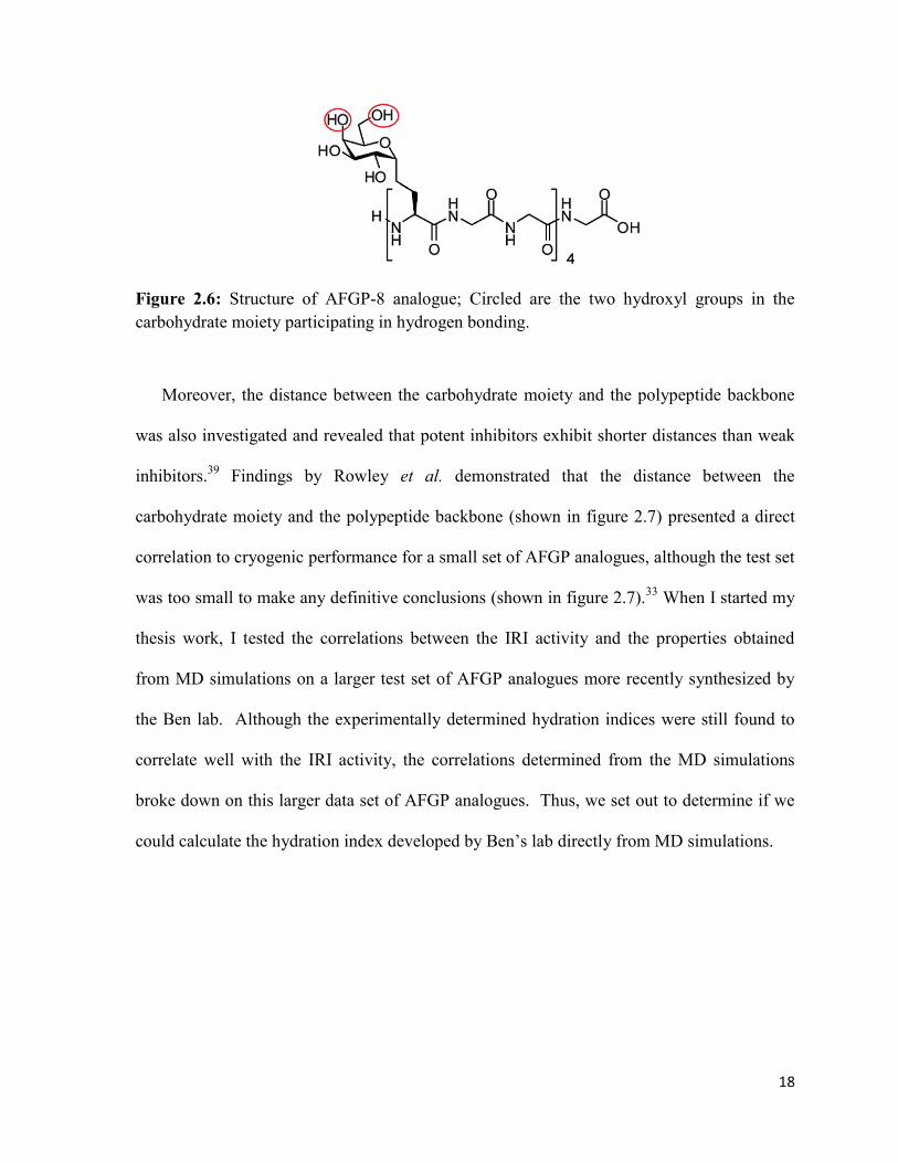
They concluded that persistent hydrogen bonding between two hydroxyl groups located in
the carbohydrate moiety was solely present in non-active AFGP analogues, whereas the IRI
active counterparts demonstrated very little hydrogen bonding (see figure 2.6). This may
indicate that the hydroxyl-water interactions may be crucial to IRI activity, in such a way
that strong hydrogen bonding between the hydroxyl groups results in weak hydroxyl-water
interactions. Therefore leaving the surrounding water undisturbed causing weak IRI
activity.39
18
Figure 2.6: Structure of AFGP-8 analogue; Circled are the two hydroxyl groups in the
carbohydrate moiety participating in hydrogen bonding.
Moreover, the distance between the carbohydrate moiety and the polypeptide backbone
was also investigated and revealed that potent inhibitors exhibit shorter distances than weak
inhibitors.39
Findings by Rowley et al. demonstrated that the distance between the
carbohydrate moiety and the polypeptide backbone (shown in figure 2.7) presented a direct
correlation to cryogenic performance for a small set of AFGP analogues, although the test set
was too small to make any definitive conclusions (shown in figure 2.7).33
When I started my
thesis work, I tested the correlations between the IRI activity and the properties obtained
from MD simulations on a larger test set of AFGP analogues more recently synthesized by
the Ben lab. Although the experimentally determined hydration indices were still found to
correlate well with the IRI activity, the correlations determined from the MD simulations
broke down on this larger data set of AFGP analogues. Thus, we set out to determine if we
could calculate the hydration index developed by Ben’s lab directly from MD simulations.

19
Figure 2.7: Snapshots of the MD conformations for 4 different analogues. Analogue 3 has
the shortest carbohydrate-backbone distance. It is also the most potent ice recrystallization
inhibitor. Reproduced from reference [39] 39
Objectives:
Since Ben and coworkers found that the IRI efficacy could be correlated with the so-
called hydration index of a AFGP analogue, the goal of my initial thesis project was to
determine if we could accurately calculate the hydration index from molecular dynamics
simulations. This would involve determining the partial molar volume and the hydration
number from such simulations. Rather than attempt to evaluate the hydration index on AFGP
analogues, our initial goal was to determine if the hydration indices could be determined
from MD simulations for the carbohydrate components of selected AFGP analogues
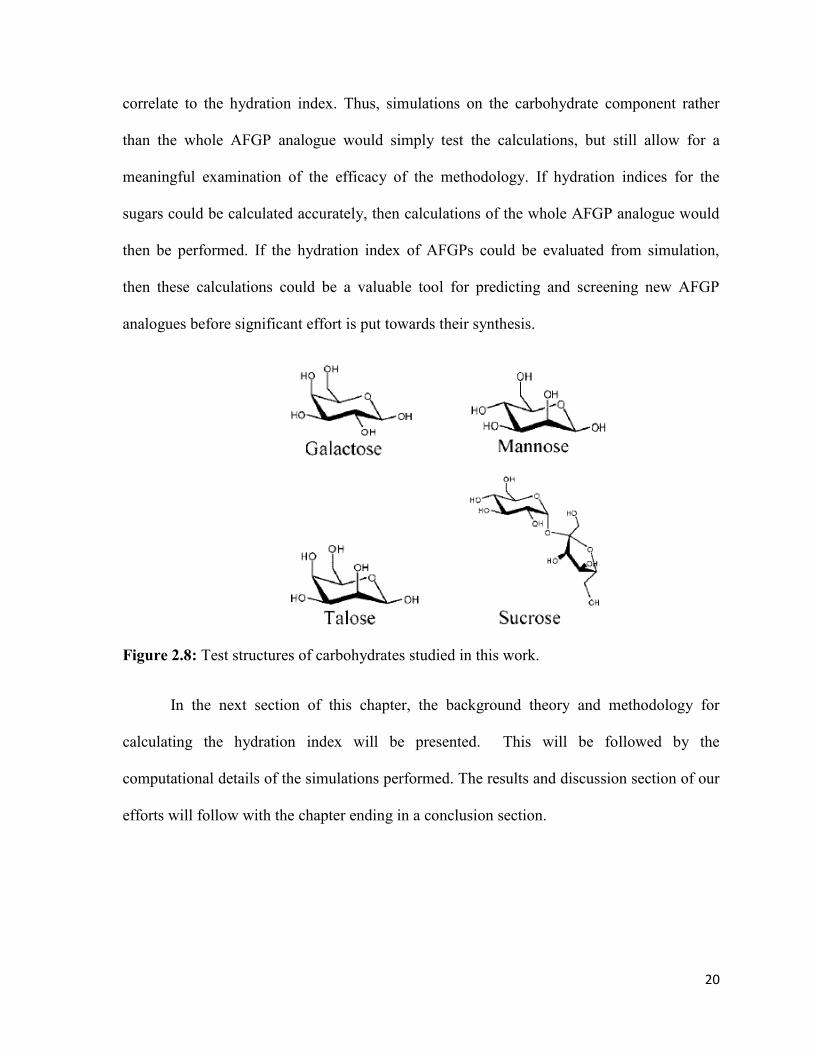
developed in the Ben lab; specifically talose, mannose, galactose, and sucrose (figure 2.8).
The carbohydrates alone also exhibit IRI activity that Ben and coworkers were also able to
20
correlate to the hydration index. Thus, simulations on the carbohydrate component rather
than the whole AFGP analogue would simply test the calculations, but still allow for a
meaningful examination of the efficacy of the methodology. If hydration indices for the
sugars could be calculated accurately, then calculations of the whole AFGP analogue would
then be performed. If the hydration index of AFGPs could be evaluated from simulation,
then these calculations could be a valuable tool for predicting and screening new AFGP
analogues before significant effort is put towards their synthesis.
Figure 2.8: Test structures of carbohydrates studied in this work.
In the next section of this chapter, the background theory and methodology for
calculating the hydration index will be presented. This will be followed by the
computational details of the simulations performed. The results and discussion section of our
efforts will follow with the chapter ending in a conclusion section.

21
Methodology
Recall, the initial goal of this work is to directly evaluate the hydration index for a set
of carbohydrates (i.e. talose, mannose, galactose and sucrose). Ben and coworkers developed
this index to correlate well to IRI activity of AFGP analogues.39
The group defines the
hydration index as:36
2.1
where is the hydration number of the solute (in our case the carbohydrate) in water and
is the partial molar volume of the solute at infinite dilution.36
First, let us dissect the
hydration index into two separate calculations, being the partial molar volume and
being the hydration number.
The initial step in this procedure is to evaluate the partial molar volume (PMV) at
infinite dilution which is equivalent to the apparent partial molar volume (volume observed
in solution depending on its mole composition).42
This property is defined by:43
( )
( )⁄ ⁄ 2.2
where and are the densities of the pure water and the carbohydrate solution,
respectively; is the molality of the carbohydrate in solution; and is the molar mass of
the carbohydrate.43
It is evident from equation 2.2 that three (3) variables are required to
directly evaluate the partial molar volume: and . First, the molality M in equation 2.2
can be easily calculated knowing the composition of the system with the following relation:42
2.3

22
where is the number of moles of solute (i.e. carbohydrate) in the solution and
is the mass of the solvent (i.e. water) in the solution. Secondly, to calculate the
partial molar volume in equation 2.2, one would need to evaluate the density, of the
carbohydrate solution. This can be accomplished by means of classical molecular dynamics
simulations of the solute in water.44
The average density value of the solution in question is
then extracted over the entirety of the simulation.44-46
This results in the direct evaluation of
(carbohydrate solution density) and (pure water density). Calculating the partial molar
volume by means of classical MD completes the first step in the procedure for determining
the hydration index.
The second step in evaluating the hydration index requires the hydration number
of equation 2.1 defined as:43
( ⁄ ) (
⁄ ) 2.4
where and in this case are the mole fractions of water and solute (carbohydrate),
respectively for the solution in question. and of equation 2.4 are the isentropic partial
molar compressibility coefficients of pure water and the carbohydrate solution,
respectively.43
The isentropic partial molar compressibility coefficient is the measure of
how compressible a solution is depending on its composition at constant entropy.42
Equation
2.4 requires the evaluation of four variables to directly calculate the hydration number
and . The mole fractions are easily calculated knowing the composition of the
system with the following relation:42
2.5
23
where represents pure water ( ) or the carbohydrate ( ), therefore is the number of
moles of the constituent of interest (pure water or carbohydrate) and is the total number
of moles in the system (i.e. moles of water in the case of pure water and moles of pure water
added to the moles of carbohydrate in the case of solutions).42
The biggest challenge in calculating the hydration index from simulation involves
determining the final variable in equation 2.4, the isentropic partial molar compressibility
coefficients, . This property is defined as:43
(
) (
) 2.6
where the variation of the volume with respect to pressure is under constant entropy .43
Unfortunately, molecular dynamics simulations at constant entropy are not standard
simulations making these calculations problematic. Fortunately, at ambient temperatures and
lower, the isentropic partial molar compressibility, , is nearly equal to the isothermal
partial molar compressibility, :47
(
) (
) (
) (
) 2.7
Figure 2.9 shows the variation of and for water as a function of temperature.47
The
isothermal partial molar compressibility is potentially more accessible to simulation as
conventional NPT ensembles (constant number of particles, pressure and temperature) could
be utilized.

24
Figure 2.9: Isothermal and adiabatic compressibilities of water. Isothermal and adiabatic
compressibilities of water are nearly equivalent at 25 °C.47
There are several literature examples that study the partial molar volume and use the
isentropic partial molar compressibility coefficients to estimate the hydration number of
carbohydrates in water. For example, Galema and coworkers experimentally estimated the
partial molar volumes and hydration numbers for a series of carbohydrates in 1991.43
The
latter study utilized the isentropic methodology presented in equation 2.2 and 2.4, and
according to their results, they provided exceptionally accurate partial molar volumes and
hydration numbers.43
Due to the accuracy of this study and the relation presented in equation
2.7, the isothermal partial molar compressibility should be a plausible approximation to the
isentropic molar compressibility at room temperature yielding similar accuracy.
Temperature, °C
Com
pres
sibi
lity,
Gpa
-1
0
Isothermal
Adiabatic
10050
0.50
0.40
25
Using classical molecular dynamics simulations in the NTP ensemble, the isothermal
partial molar compressibility coefficients can be determined more readily by the fluctuation
relationship with the following equation:48
(
) (
) ⟨
⟩ 2.8
Where is the average variance of the volume for a given simulation; is the Maxwell-
Boltzmann constant; is the temperature; and is the average volume of the
simulation.48
Once the value of is evaluated using classical molecular dynamics
simulations, it can be substituted in equation 2.4 along with the mole fractions to evaluate the
hydration number.
Recall, to directly evaluate the hydration index (equation 2.1) the partial molar
volume (equation 2.2) and the hydration number (equation 2.4) are required. The
methodology detailed above demonstrates the procedure to directly evaluate the hydration
index.
More recently, Voth and coworkers have evaluated the isothermal partial molar
compressibility coefficients of different water models and found that most models accurately
predict this value.49
Voth and coworkers attempted to evaluate the isothermal partial molar
compressibility more directly by evaluating the variation of the volume with respect to
pressure using the finite difference approximation given by:49
(
) (
) (
⁄
)
2.9
where is the density corresponding to pressure and is the density corresponding to
pressure .49
Unlike the fluctuation method, this method requires multiple simulations to

26
evaluate the isothermal partial molar compressibility coefficients. Finite difference
procedures begin by utilizing a typical NPT simulation at ambient conditions to extract the
equilibrium density of the system.49
In addition, two NVT ensemble simulations
(constant number of particles, volume and temperature) are required.49
One equates to
density defined as: 49
g/cm3
2.10
the other simulation equates to density defined as: 49
g/cm3
2.11
These simulations provide the necessary data to evaluate using equation 2.9.
Pressures and can be extracted from the simulations of and , respectively. This
method provides an alternative route for evaluating the hydration index with the isothermal
partial molar compressibility.
Both the fluctuation approach and the finite difference approach will be
investigated in this work as to standardize the procedure for these types of studies.

27
Computational details
Description of model systems
The main objective in this work is to determine the hydration index of various
carbohydrates (i.e. Glactose, mannose, talose, sucrose) using classical molecular dynamics
simulations. This section will provide the specifications necessary to reproduce the
simulations used in this work.
Figure 2.10: Snapshot of a simulation cell of a solvated carbohydrate surrounded by TIP3P
water. Boxed area represents a close up of the solvated carbohydrate in the simulation cell.
The simulations in this project were performed using the AMBER-9 simulation
package and consist of a single carbohydrate (i.e. Glactose, mannose, talose, sucrose)
solvated by water as depicted in figure 2.10. The initial step in creating these systems
requires the insertion of the carbohydrate at the center of the orthorombic simulation box
with cell dimensions of 32.0x33.0x34.0 Å. All carbohydrate configurations were built using
Glycam’s Carbohydrate 3D Structure Predictor on the glycam website.50
This supplied the
necessary pdb files containing carbohydrate structures for our simulations.50
The next step in

28
constructing our simulations requires the solvation of the carbohydrates with TIP3P water
using the built-in AMBER Solvate Box program. The latter program incrementally adds
water molecules into the simulation box provided while crosschecking a designated radius
around the newly inserted water molecule ensuring that there is no overlap with any other
molecules in the simulation cell.45
A 16 Å parameter describing the distance between the
carbohydrate and the edge of the simulation box was used with the solvate box program,
adding roughly 3300-3350 water molecules. Periodic boundary conditions were utilized to
approximate the bulk solution.
A complication for these simulations is the necessity of infinite dilution. Due to the
nature of this study, the properties of interest (i.e. PMV) depend solely on the contributions
of one carbohydrate interacting with its hydration shell. To truly satisfy infinite dilution
(defined as no solute-solute interactions) the carbohydrates must not directly (carbohydrate-
carbohydrate interaction) or indirectly (hydration shell-hydration shell interaction) interact
with one another.51
As previously mentioned, periodic boundary conditions replicate the
system creating multiple carbohydrates in the simulation. Altough, non-bonded cut-offs can
be used to eliminate the Van der Waals interactions between solute molecules, there will still
be long ranged electrostatic interactions between periodic images.
The electrostatics in the simulation were governed by the Point-Charge model
derived by using a standard AM1-BCC method reproducing RESP charges52,53
calculated at
a Hartree-Fock/6-31G* level of accuracy. The Glycam force field developed by Woods and
co-workers is used to describe inter and intra molecular interactions within and between

29
carbohydrates.54
Glycam is a specialized force field developed for carbohydrates.54
A typical
TIP3P rigid potential was used to define water interactions in the system.55
Simulations were also performed using the DL_POLY 2.17 simulation package. For
reasons described later on in this work, DL_POLY was used to simulate the alcohols
propanol, propanediol, hexanol, and hexanediol in water. Simulations consisted of a single
alcohol solvated by water in a cubic simulation cell of length 45.0 Å. Alcohol structures
optimized at the empirical level using the Generalized Amber Force Field were used for all
simulations. Once again, the alcohols were then solvated with TIP3P water, this time using
the built-in DL_POLY Water Add program. Unlike AMBER’s Solvate Box program,
DL_POLY’s Water Add requires only simulation cell vectors, inserting roughly 1950-3350
water molecules in our simulation cell. The program does so by replicating the simulation
cell with the same dimensions and fills it with water molecules. The next step in the Water
Add Program combines the simulation cell containing the alcohol and the simulation cell
containing the water and systematically removes any water molecules that overlap with the
solute.46
Unlike the Amber model, DL_POLY simulations utilized a different force field to
define inter and intra molecular interactions. Instead of the Glycam force field, the
Generalized AMBER Force Field was used to describe inter and intra molecular interactions
within and between alcohols.56
GAFF is a more generalized force field that can treat a wider
range of general organic compounds.56
Furthermore, the performance and efficiency of the
GAFF parameters have been successfully tested to properly represent the conformations,
energies and dynamical properties for multiple organic species including alcohols.56
Finally,
periodic boundary conditions, point charges, Van der Waals interactions, the water model
used in the AMBER simulations were used with DL_POLY.

30
The Amber & DL_POLY simulation packages used in this study utilize the Leap
Frog-Verlet algorithm to integrate the equations of motion.45
The initial configurations
generated from Amber and DL_POLY solvation codes were first optimized. For the Amber
calculations on the carbohydrates, the AMBER-9 simulation package was used. For these
simulations, the systems were first equilibrated under constant temperature and pressure
conditions for 100 ps. The simulation times for the production runs were a nanosecond or
greater. These simulations were performed under ambient conditions with temperatures and
pressures set to 293 K and 1 atm, respectively. All bonds involving hydrogen atoms were
frozen using the SHAKE algorithm, to allow for the use of a large timestep of 1.0 fs. Ewald
summations were used in all simulations to quickly treat long ranged Coulombic interactions.
The Nosé/Hoover thermostat/barostat was utilized in this work with a thermostat constant of
5.0 ps-1
, and a barostat constant of 0.5 ps. Finally, a 12 Å non-bonded cutoff was employed
to reduce the number of non-bonded interactions.
In addition to NPT simulations, NVT simulations were used in this study to
investigate two (2) different calculation methodologies for determining the partial molar
compressibility coefficients. The fluctuation method presented by Galema and co-workers
was evaluated in the NPT ensemble and the finite difference method presented by Voth was
evaluated in the NVT ensemble. For the NVT simulations, the simulation parameters were
identical to those previously mentioned except that the volume was fixed in the simulations.
As previously mentioned, the finite difference method requires multiple simulations,
one simulation in the NPT ensemble providing the equilibrium density, and two (2)
simulations in the NVT ensemble at different densities. These two different simulations were
performed at slightly different densities ( defined as g/cm3 and

31
defined as g/cm3) where is the density of the system at equilibrium
determined from the NPT simulation. The resulting configuration from the NPT simulations
served as an initial configuration for the NVT simulations. Similar to NPT simulation, an
equilibration run in the NVT ensemble served to make the transition between the NPT
ensemble and the NVT ensemble smoother.
32
Results and discussion
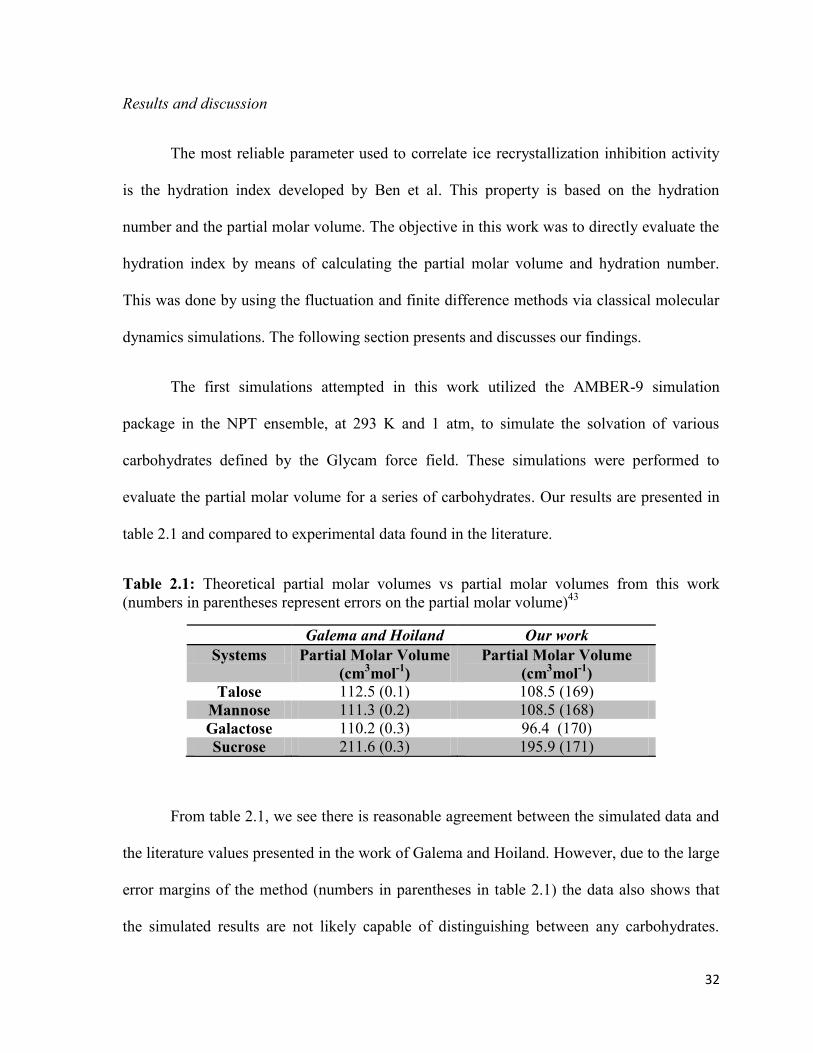
The most reliable parameter used to correlate ice recrystallization inhibition activity
is the hydration index developed by Ben et al. This property is based on the hydration
number and the partial molar volume. The objective in this work was to directly evaluate the
hydration index by means of calculating the partial molar volume and hydration number.
This was done by using the fluctuation and finite difference methods via classical molecular
dynamics simulations. The following section presents and discusses our findings.
The first simulations attempted in this work utilized the AMBER-9 simulation
package in the NPT ensemble, at 293 K and 1 atm, to simulate the solvation of various
carbohydrates defined by the Glycam force field. These simulations were performed to
evaluate the partial molar volume for a series of carbohydrates. Our results are presented in
table 2.1 and compared to experimental data found in the literature.
Table 2.1: Theoretical partial molar volumes vs partial molar volumes from this work
(numbers in parentheses represent errors on the partial molar volume)43
From table 2.1, we see there is reasonable agreement between the simulated data and
the literature values presented in the work of Galema and Hoiland. However, due to the large
error margins of the method (numbers in parentheses in table 2.1) the data also shows that
the simulated results are not likely capable of distinguishing between any carbohydrates.
Galema and Hoiland Our work
Systems Partial Molar Volume
(cm3mol
-1)
Partial Molar Volume
(cm3mol
-1)
Talose 112.5 (0.1) 108.5 (169)
Mannose 111.3 (0.2) 108.5 (168)
Galactose 110.2 (0.3) 96.4 (170)
Sucrose 211.6 (0.3) 195.9 (171)

33
These results led to further investigation and revealed a fundamental problem with the
density extracted from our simulations. It was observed that the density values for different
carbohydrates are only slightly different (on the order of 10-4
). Consequently, density errors
on a similar order (10-4
) produce indistinguishable differences between the carbohydrates.
Due to the strong dependence of the partial molar volume to the density (see equation 2.2),
the PMV values become erroneous.
To address this problem, an understanding of the density inaccuracy is required. The
density is directly proportional to volume and pressure, thus any unexpected fluctuations can
strongly affect this value. In fact, this is precisely the case in our NTP simulations. Pressure
fluctuations are occurring on such a large scale that errors on the density are relatively large
(10-3
). Errors such as these render our simulations untenable for evaluating the partial molar
volume. Therefore, more precise and accurate means to regulate the pressure in the system is
necessary. Regulating the barostat relaxation constant proved futile in the attempt to obtain
more converged densities. As a result of our previous efforts, it was thought that the problem
lay in the Langevin thermostat/barostat used in AMBER. This thermostat/barostat does not
rigorously sample the NPT ensemble due to the nature of the scaling.45
The technique
randomly selects one molecule and scales its kinetic energy to regulate the changes in
temperature and pressure.45
This results in the occurrence of potentially unphysical
equilibrium behaviour and it was thought that this may be causing problems in the
convergence of the densities.45
Another common thermostat/barostat method used in classical molecular dynamics
simulations is the Nosé/Hoover method.46
This method scales the kinetic energy of all the
molecules as to formally sample the NPT ensemble.46
Unfortunately, this thermostat/barostat

34
is not implemented in the AMBER-9 simulation package. For this reason, the DL_POLY
simulation package, which utilizes the Nosé/hoover barostat/thermostat, was used for further
calculations. Moreover, it was thought that the imprecision in the density is due to the
pressure regulation in AMBER. Another contributing factor to the erratic pressure can also
be a result of the ill-defined force field used to describe intra and inter molecular
interactions. Although the Glycam force is optimized for treating carbohydrates, these
molecules are notoriously difficult to simulate, in part due to their conformational variability.
To more easily determine the sources of error in calculating the partial molar volume, we
decided to simulate simple alcohols which are expected to have more refined and accurate
force fields. The previous changes in the force field, simulation package, and
thermostat/barostat should eliminate all variables that can result in unreliable pressure.
Therefore, accurate densities and thus partial molar volumes can be extracted from future
simulations.
The remainder of the simulations performed in this study utilized the DL_POLY 2.17
simulation package along with the Generalized Amber Force Field and Nosé/Hoover
thermostat/barostat to simulate the solvation of various alcohols (i.e. propanol, propanediol,
hexanol and hexanediol) at 293 K and 1 atm. Partial molar volume results are presented in
table 2.2 and compared to experimental data found in the literature.
Table 2.2: Theoretical partial molar volumes vs partial molar volumes from this work (numbers
in parentheses are errors on the partial molar volume)51
Hoiland Our work
Systems Partial molar volume (lit.)
(cm-3 mol-1)
Partial molar volume (calc.)
(cm-3 mol-1)
Propan-1-ol 70.65 (0.05) 56.61 (202)
Propanediol-1,3 71.93 (0.05) 51.73 (152)
Hexan-1-ol 117.96 (0.05) 72.24 (159)
Hexanediol-1,3 120.01 (0.05) 95.05 (158)

35
Unfortunately, results presented in Table 2.2 show clear discrepancies between the
simulated data in this work and the literature values presented in the work of Hoiland.51
Similar to the carbohydrate results in Table 2.1, the error margins on the partial molar
volume of the alcohols prevent us from distinguishing between molecules. Further
investigation revealed the same density related problem as the AMBER calculations on
carbohydrates. In the case of the alcohols, the density errors are also on the orders of 10-3
whereas the density differences between different alcohols are only on the order of 10-4
. This
is illustrated in figure 2.11.
Figure 2.11: Density error analysis for all alcohols extracted from DL_POLY simulations
using GAFF and the Nosé/Hoover thermostat/barostat. Density error bars are shown for all
alcohols. It is clear that all densities are within error making them indistinguishable between
one another.
The reoccurring difficulties with the density inspired a literature investigation on both
experimental and computational studies attempting to determined partial molar volumes of
molecules. Among multiple studies, we discovered that all evaluations of the partial molar
volumes are conducted at concentrations much larger (3 to 6 times) than the concentration
0.984
0.986
0.988
0.99
0.992
0.994
0.996
0.998
Den
sity
(g/c
m3)
Alcohols
Alcohol Densities
Pure water Propanol Propanediol Hexanol Hexanediol

36
used in this work (infinite dilution 0.0177 molal).59-62
Typical molal concentrations found in
the literature vary anywhere between 0.05 and 0.1 molal resulting in accurate PMV results
experimentally.59-62
However, these concentrations are no longer considered infinite dilution,
therefore solute-solute interactions must be accounted for while evaluating the partial molar
volume. Usually this is accomplished by measuring the density for a series of different
concentrations and extrapolating to infinite dilution. Figure 2.12 and table 2.3 summarize our
efforts in dealing with larger concentrations in hopes of achieving better PMV accuracies.
Simulations were no longer performed at infinite dilution; instead specific molal
concentrations used to determine the partial molar volume experimentally were replicated in
hopes of obtaining greater accuracies.
Figure 2.12: Partial molar volume of propanol at different concentrations. Dotted line
represents the experimental literature value of the partial molar volume of propanol at
infinite dilution. Solid line represents the extrapolation to infinite dilution from our
simulations.
50
55
60
65
70
75
0 0.05 0.1 0.15 0.2 0.25
PM
V (
cm3/m
ol)
Molal concentration (mol/kg)
Partial molar volume at experimental concentrations
y = 147.79x + 52.76

37
Table 2.3: Partial molar volume of propanol at different simulated concentrations.
Number of alcohols
molecules
Number of water
molecules
Molality (mol/kg) Partial molar
volume (cm3/mol)
1 3143 0.0177 56.6
1 2116 0.0264 54.8
2 3921 0.0278 57.7
2 1934 0.0569 60.5
3 1934 0.0862 66.0
4 1934 0.1089 66.8
5 1934 0.1435 65.6
7 1934 0.2017 67.0
Figure 2.12 illustrates the partial molar volume extracted from the simulations
submitted at different concentrations. It is clear from the results that the limiting
concentration for classical molecular dynamics simulations is reached at a concentration of
roughly 0.0862 molal. The partial molar volume of propanol converges to a value of ~ 66.0
cm3/mol. The dotted line in figure 2.12 represents the experimental literature value of the
PMV for propanol at infinite dilution (70.65 cm3/mol). Unfortunately, the literature value
and our calculated value are not very comparable (20% error). Errors such as these are not
acceptable especially for evaluating the PMV, where very accurate and precise values are
required in order to distinguish between solutes that are very similar in structure (i.e.
propanol vs propanediol). More importantly, the partial molar volume difference between
stereochemically different carbohydrates such as galactose and mannose will not be
accessible.
Due to the increased concentration required to achieve the detection limit, PMV
results extracted from MD simulations are further discredited. Although this increase in
concentration generated more accurate partial molar volumes of 66.0 cm3/mol as opposed to
56.61 cm3/mol, simulations performed at the limiting concentration no longer satisfy the

38
condition of infinite dilution. Figure 2.13 represents propanol at concentrations in the
detection limit of molecular dynamics simulations. It is clear from this figure that solute-
solute interactions are present in the system, thus the partial molar volume extracted from
these simulations are not representative of the PMV at infinite dilution. To obtain a more
representative value for the partial molar volume at infinite dilution, the data evaluated for
the different concentrations must be extrapolated. The extrapolation (solid line) is shown in
figure 2.12, leading to a calculated PMV of 52.76 cm3/mol.
Figure 2.13: Simulation cell illustrating solute-solute (propanol) interactions at the limiting
concentration of molecular dynamics simulations; water molecules have been omitted for
clarity. It is evident that the alcohols are grouping together.
In addition to our study, a thorough literature review revealed many sources studying
solvated alcohols, alcanes, and carbohydrates with molecular dynamics simulations.59-62
These studies also determined volumetric properties such as partial molar volume and
revealed similar problems in reproducing experimental partial molar volumes. In-depth
investigations of these studies reveal similar density issues as our research.59-62
This confirms
that the accuracy obtained in this work is the limit of molecular dynamics simulations. 59-62

39
Unfortunately, simulated densities are not comparable to experimental results. Consequently,
the volumetric properties of interest such as the PMV will be inaccurate. These inaccuracies
will translate directly to inaccuracies in the hydration index making any correlations to the
ice recrystallization inhibition activity impossible. These results show that MD simulations
cannot be used to calculate the hydration indices using the methods outlined.
40
Conclusion
Previously, Ben et al observed that ice recrystallization inhibition efficacy is
correlated to the hydration index. This parameter is based on the partial molar volume and
hydration number for a prospective cryoprotectant. Classical molecular dynamics
simulations were used to investigate these volumetric properties for carbohydrates such as
galactose, mannose, talose, sucrose, and alcohols including propanol propanediol, hexanol
and hexanediol. These simulations were performed in hopes of facilitating and standardizing
the screening protocol of possible novel antifreeze compounds. After 8 months of rigorous
testing, a clear conclusion can be drawn.
The use of classical molecular dynamics simulations to investigate volumetric
properties such as the partial molar volume and hydration number is not possible due to the
heavy dependence on density. The density of a solution is highly dependent on the
concentration of the solute in question as is the partial molar volume. This work illustrates
that the accuracy and precision of the density extracted from simulations is not sufficient to
distinguish between similar compounds.
The partial molar volume of a compound relies fundamentally on one variable
property; density. These densities can be extracted by simulating the solutions of interest.
However, classical molecular dynamics simulations demonstrate a detection limit which is
the threshold for distinguishing similar properties of different species. Unfortunately, the
detection limit for the density in classical molecular dynamics simulations is much greater
than the density differences of different species at infinite dilution, thus accurate partial
molar volumes cannot be extracted.

41
To conclude, this work demonstrates clearly that current classical molecular
dynamics technology cannot probe the volumetric properties of interest with sufficient
accuracy to aid in the research and development of novel cryoprotectants.

42
(1) Hafez, T. F., B.; Baust J. G.; Baust J. M. CRC press: Boca Raton 2007, 197-
210.
(2) Transplantation, U. S. G. I. o. O. a. T. D. a. http://organdonor.gov/ 2011.
(3) Mazur, P. American Journal of Physiology 1984, 247, C125-C142.
(4) Mazur, P.; Leibo, S. P.; Chu, E. H. Y. Experimental Cell Research 1972, 71,
345-&.
(5) Fowler, A.; Toner, M. In Cell Injury: Mechanisms, Responses, and Repair;
New York Acad Sciences: New York, 2005; Vol. 1066, p 119-135.
(6) Eroglu, A.; Bailey, S. E.; Toner, M.; Toth, T. L. Biology of Reproduction
2009, 80, 70-78.
(7) Hossain, A. M.; Osuamkpe, C. O. Archives of Andrology 2007, 53, 99-103.
(8) Hunter, J. E.; Bernard, A.; Fuller, B.; Amso, N.; Shaw, R. W. Human
Reproduction (Oxford) 1991, 6, 1460-1465.
(9) Mondal, B. Cell and Tissue Banking 2009, 10, 341-344.
(10) Wezeman, F. H.; Guzzino, K. M. Cryobiology 1986, 23, 81-87.
(11) Whittingham, D. G. Journal of Reproduction and Fertility 1977, 49, 89-94.
(12) Davis, J. M.; Rowley, S. D.; Braine, H. G.; Piantadosi, S.; Santos, G. W.
Blood 1990, 75, 781-786.
(13) Elmoazzen, H. Y.; Poovadan, A.; Law, G. K.; Elliott, J. A. W.; McGann, L.
E.; Jomha, N. M. Cell and Tissue Banking 2007, 8, 125-133.
(14) Liseth, K. A., J. F.; Bjorsvik, S.; Grottebo, K.; Bruserud, O. Cryotherapy
2005, 7, 328-333.
(15) Ohlendorf, C.; Tomford, W. W.; Mankin, H. J. Journal of Orthopaedic
Research 1996, 14, 413-416.
(16) Gage, A. A. B., J. Cryobiology 1998, 61, 3149-3158.
(17) Turnbull, D. Solid State Physics-Advances in Research and Applications
1956, 3, 225-306.
(18) J.M., B. Cell preservation technology 2002, 1, 17-31.
(19) Turnbull, D. Journal of Physical Chemistry 1962, 66, 609-&.

43
(20) DeVries, A. L. Biochemical and Biophysical perspectives in marine biology
1974, 289-330.
(21) Duman, J. G.; Olsen, T. M. Cryobiology 1993, 30, 322-328.
(22) Graham, L. A.; Liou, Y. C.; Walker, V. K.; Davies, P. L. Nature 1997, 388,
727-728.
(23) Yeh, Y.; Feeney, R. E. Chemical Reviews 1996, 96, 601-617.
(24) Devries, A. L.; Wohlschl.De Science 1969, 163, 1073-&.
(25) Devries, A. L. K., S.K.; Feeney, R.E. Journal of biological chemistry 1970,
245, 2901-2908.
(26) Gordon, M. S.; Scholander, P. F.; Amdur, B. H. Biological Bulletin 1962,
122, 52-&.
(27) Scholander, P. F.; Vandam, L.; Kanwisher, J. W.; Hammel, H. T.; Gordon, M.
S. Journal of Cellular and Comparative Physiology 1957, 49, 5-24.
(28) Duman, J. G.; Devries, A. L. Cryobiology 1972, 9, 469-472.
(29) Lin, Y.; Devries, A. L.; Duman, J. G. Biochemical and Biophysical Research
Communications 1972, 46, 87-&.
(30) Raymond, J. A.; Devries, A. L. Cryobiology 1972, 9, 541-547.
(31) Scholand.Pf; Maggert, J. E. Cryobiology 1971, 8, 371-&.
(32) Harding, M. M.; Anderberg, P. I.; Haymet, A. D. J. European Journal of
Biochemistry 2003, 270, 1381-1392.
(33) Tam, R. Y.; Rowley, C. N.; Petrov, I.; Zhang, T. Y.; Afagh, N. A.; Woo, T.
K.; Ben, R. N. Journal of the American Chemical Society 2009, 131, 15745-15753.
(34) Feeney, R. E.; Burcham, T. S.; Yeh, Y. Annual Review of Biophysics and
Biophysical Chemistry 1986, 15, 59-78.
(35) Fletcher, G. L.; Hew, C. L.; Davies, P. L. Annual Review of Physiology 2001,
63, 359-390.
(36) Tam, R. Y.; Ferreira, S. S.; Czechura, P.; Chaytor, J. L.; Ben, R. N. Journal of
the American Chemical Society 2008, 130, 17494-17501.
(37) Karim, O. A.; Haymet, A. D. J. Chemical Physics Letters 1987, 138, 531-534.

44
(38) Sadtchenko, V.; Ewing, G. E. Journal of Chemical Physics 2002, 116, 4686-
4697.
(39) Czechura, P.; Tam, R. Y.; Dimitrijevic, E.; Murphy, A. V.; Ben, R. N.
Journal of the American Chemical Society 2008, 130, 2928-2929.
(40) Uchida, T.; Nagayama, M.; Shibayama, T.; Gohara, K. Journal of Crystal
Growth 2007, 299, 125-135.
(41) Liu, S. H.; Ben, R. N. Organic Letters 2005, 7, 2385-2388.
(42) Petrucci, R. H. H., F.G.; Madura, J.D.; Bissonnette, C. Pearson 2011, 10,
214,560.
(43) Galema, S. A.; Hoiland, H. Journal of Physical Chemistry 1991, 95, 5321-
5326.
(44) Leach, A. R. Prentice Hall 1996.
(45) Amber9 Reference manual.
(46) DL_POLY2.17 Reference manual.
(47) Zemansky, M. W. D., R.W. McGraw-Hill Book Company 1981, 6, 238.
(48) McQuarrie, D. A. Harper and Row 1976.
(49) Wu, Y. J.; Tepper, H. L.; Voth, G. A. Journal of Chemical Physics 2006, 124,
12.
(50) http://glycam.ccrc.uga.edu/ccrc/carbohydrates/cb_newbuilder.jsp.
(51) Hoiland, H. Journal of Solution Chemistry 1980, 9, 857-866.
(52) Cieplak, P.; Cornell, W. D.; Bayly, C.; Kollman, P. A. Journal of
Computational Chemistry 1995, 16, 1357-1377.
(53) Cornell, W. D.; Cieplak, P.; Bayly, C. I.; Kollman, P. A. Journal of the
American Chemical Society 1993, 115, 9620-9631.
(54) Woods, R. J.; Dwek, R. A.; Edge, C. J.; Fraserreid, B. Journal of Physical
Chemistry 1995, 99, 3832-3846.
(55) Jorgensen, W. L.; Chandrasekhar, J.; Madura, J. D.; Impey, R. W.; Klein, M.
L. Journal of Chemical Physics 1983, 79, 926-935.

45
(56) Wang, J. M.; Wolf, R. M.; Caldwell, J. W.; Kollman, P. A.; Case, D. A.
Journal of Computational Chemistry 2004, 25, 1157-1174.
(57) Case, D. A.; Cheatham, T. E.; Darden, T.; Gohlke, H.; Luo, R.; Merz, K. M.;
Onufriev, A.; Simmerling, C.; Wang, B.; Woods, R. J. Journal of Computational Chemistry
2005, 26, 1668-1688.
(58) Case, D. A. e. a. University of California 2006, San Francisco.
(59) Avdeev, M. V.; Bodnarchuk, I. A.; Petrenko, V. I.; Kholmurodov, K. T.;
Yaradaikin, S. P. Russian Journal of Physical Chemistry A 2009, 83, 1129-1133.
(60) Romero, C. M.; Paez, M. S.; Arteaga, J. C.; Romero, M. A.; Negrete, F.
Journal of Chemical Thermodynamics 2007, 39, 1101-1109.
(61) Romero, C. M.; Paez, M. S.; Perez, D. Journal of Chemical Thermodynamics
2008, 40, 1645-1653.
(62) Sangwai, A. V.; Ashbaugh, H. S. Industrial & Engineering Chemistry
Research 2008, 47, 5169-5174.
(63) Baruch, E.; Belostotskii, A. M.; Mastai, Y. Journal of Molecular Structure
2008, 874, 170-177.
(64) Furuki, T. Carbohydrate Research 2000, 323, 185-191.
(65) Furuki, T. Carbohydrate Research 2002, 337, 441-450.
(66) Galema, S. A.; Howard, E.; Engberts, J.; Grigera, J. R. Carbohydrate
Research 1994, 265, 215-225.

46
Chapter 3: Investigating the feasibility of sI clathrate hydrates as carbon capture tools
Introduction
Carbon capture and storage (CCS) represents a serious strategy to reduce the
environmental impact of energy production by capturing CO2 from the combustion gas and
permanently storing it. The development of new carbon capture materials and carbon capture
protocols are imperative to the struggle of mitigating the ever increasing temperature of
earth’s atmosphere. For over two hundred years, mankind has been releasing increasing
amounts of greenhouse gases (GHG) such as methane, carbon oxides, nitrous oxides and
chloro/fluorocarbons into the atmosphere1. These gases are capable of retaining infrared (IR)
radiation inside earth’s atmosphere causing temperatures to climb.1 The increased release of
GHG in the last century alone has resulted in a 0.74 °C rise in average global temperature.2
Among many concerns associated with the rise in temperature, global sea levels and
vegetation viability are the most important. The aforementioned increase in temperature has
resulted in a 17 cm increase in average global sea levels due to thawing polar ice caps and
glaciers.2 Consequently, global warming has become one of the leading environmental and
political concerns today. Many political efforts have attempted to regulate the latter by
implementing strategies such as the Kyoto protocol established in 1997 by the United
Nations Framework Convention on Climate Change (UNFCCC).3,4
The latter requires those
whom have ratified to reduce their GHG emissions by 5.2 % of their 1990 emission level.3,4
For these reasons, carbon capture and storage techniques/materials play an essential role in
the future of earth’s climate.

47
World energy demands and the cost (real and perceived) associated with the start-up
of new technologies for energy production mean that fossil fuels will continue to be used for
power generation. Therefore, high levels of CO2 will continue to be emitted from flue stacks
in combustion plants despite the many concerns raised about global warming. Coal
combustion for power generation alone produces 7 gigatonnes of anthropogenic CO2 per
year.5 This is equivalent to 40% of all anthropogenic CO2 emission yearly.
5 Fortunately, CO2
is one of the weaker GHGs as it can only absorb a small spectrum of infrared radiation.
Although CO2 is not considered a particularly potent greenhouse gas (GHG), its importance
is due to its escalating concentration in the atmosphere making it the largest contributor of
anthropogenic GHG to global warming. For this reason, CCS has attracted serious attention.
Numerous pilot programs exist in the struggle for carbon capture and storage. For example,
some commercial coal plants have been retrofitted with CO2 carbon capture technology.
Nonetheless, large scale CCS is not yet realized.
At the moment, the most significant barrier to large scale CCS from coal burning
power plants is that low energy and cost effective CO2 scrubbing technologies do not exist.
However, several methodologies are being explored and developed. One CO2 scrubbing
method widely used today is based on aqueous amines, such as mono or diethanolamine.
These solutions are used to capture the CO2 from the flue gas by means of chemisorption.6
Once CO2 and the aqueous amine interact, a chemical reaction can occur. This process is
based on the following reactions where R is the remaining atoms in a typical amine:7
3.1
3.2

48
Although presently the most commonly used CCS method, in order to recover the
liquid amine sorbent, heating of the solution is required. This process is energetically costly.
Furthermore, the liquid amine solution is toxic, corrosive, and degrades over time due to
irreversible side reactions with other flue gases. Consequently, the aqueous amine solvent
must be replaced at a rate of eight pounds per ton of CO2 captured, adding to the overall cost
of clean energy production.6 Today, incorporating aqueous amine scrubber technology in
power plants usually translates to a drop in power generating efficiency (roughly 30 %) per
combustible fuel. This is due to the parasitic energy load of the carbon capture mechanism
making alternatives to this approach desirable.8
Another technology that has received great attention is the use of nanoporous solids
to capture CO2 (g) in flue gas post-combustion. Such solids include zeolites (Zeolitic
Imidazolate Framework) and metal organic frameworks (MOFs). Unlike liquid amines,
nanoporous solids interact with the flue gas by means of adsorption.9,10
These materials are
porous crystalline solids with well-defined cavities. They can be tuned to tailor pore size,
accessibility, gas selectivity, and gas uptake simply by substituting the fundamental building
blocks in the framework such as metal linkers and organic ligands. Flue gas derived from the
coal burning process is allowed to diffuse through a compartment containing the nanoporous
material. In which case, the gases (i.e. CO2) have the opportunity to adsorb to certain sites in
the framework by means of non-bonded (dispersion and/or electrostatics) interactions. The
CO2 saturated material can then be regenerated by multiple means such as pressure swing or
temperature swing techniques. The most common method utilizes a combination of the two
techniques. In these processes, adsorption usually occurs at a given temperature and pressure.

49
However, desorption of CO2 is forced at greater temperatures and lower pressures than those
used for adsorption. The newly freed carbon dioxide gas can now be compressed, stored or
transported in a separate container. The desorption process regenerates the nanoporous solid
for recycled use in future capture. A schematic representation of a zeolite containing
adsorbed CO2 is exemplified in figure 3.1.
Figure 3.1: SiO2, silicate structure (zeolite). Carbon dioxide fills the micro-pores of the
zeolite under pressure. Reproduced from reference [11] 11
A problem with the MOF materials (other than their high cost of production) is that
they are susceptible to being poisoned by water which is a major combustion product.12
Moreover, even if the MOF is water stable, it must be significantly more selective for CO2
than water to effectively capture, separate or store carbon dioxide.12
One solution for dealing
with water is to use a hydrophobic MOF. However, the MOF must also be selective for CO2
over other non-polar combustion gases such as N2.12

50
Current technologies for capture and storage have much room for improvement. The
challenge now resides in researching and developing novel CCS materials and protocols that
can efficiently and effectively remove and store carbon dioxide from the flue gas in coal
combustion plants. The development of these technologies are of great importance and
crucial in the fight against global warming.
Figure 3.2: Single clathrate hydrate cage encapsulating a methane molecule. Hydrogen
bonds between water molecules are represented by dotted lines.
Recently, it has been proposed to use the clathrate hydrate formation potential of
CO2(g) gas under pressure (10-30 bar at 273 K) as a means of CO2 (g) capture from
combustion flue streams.13,14
At sufficiently high pressures (10 bar) and low temperatures
(below 300 K), water begins to form structured crystalline cages around non-polar molecules
(i.e. CO2) called clathrate hydrates (see figure 3.2).15
Considering ambient conditions, the
latter combination of molecules would result in an arrangement such that the non-polar-polar
interactions are minimized consequently creating two separate phases with an interacting
interface.16
However, at high pressures and low temperatures the water molecules form
ordered cages around the non-polar molecules. These cages form in such a way that
maximizes the hydrogen bonds between water molecules and as a result minimizes the

51
number of interactions with the guest (non-polar) molecule. Figure 3.2 shows the hydrogen
bonding network of the clathrate hydrates.
There are two advantages of using clathrate hydrates instead of other novel
technologies for CO2 (g) capture. The first being that the only material needed to capture the
gas is water and no other hazardous or expensive materials are involved. The second
advantage is that this method is not poisoned by water but rather uses water to capture the
gas. Thus, the abundant H2O found in flue gas will not pose any problems to the operation.
Figure 3.3 depicts a plausible clathrate hydrate process for carbon capture. This model can
theoretically be retrofitted to existing flue stacks in coal combustion plants. Unfortunately,
one problem with using clathrates as carbon capture tools is that pressurizing the flue gas to
pressures that promote the spontaneous clathrate formation is energetically costly. At the
moment, it is still unclear whether or not this process can be optimized to reduce operation
costs. Nonetheless, clathrate hydrate based CO2 scrubbing processes have been proposed and
studied.
Figure 3.3: Proposed clathrate hydrate apparatus for CO2 recovery from flue gas exhausted
from coal combustion plants. Operational temperature for this apparatus is 273 K.
Operational pressure for gas hydrate process 1, 2, and 3 are 10, 5, and 2.5 bar, respectively.
Reproduced from reference [17] 17

52
Understanding how impurities (gases other than CO2) present in the flue gas may
influence the formation of CO2 clathrate hydrates is important for using these materials for
both carbon capture and storage. These impurities may disrupt CO2 clathrate formation
and/or may impede CO2 selectivity. For example, Beeskow and coworkers recently studied
the effects of 1% SO2 and NO2 impurities on the CO2 hydrate formation process.18
They
found an enrichment of SO2 in the hydrate phase compared to the gas concentration, which
suggests that clathrate hydrate formation also removes these unwanted contaminants from
the flue. It was suggested to further investigate the influence of these impurities because they
may present some useful features such as promoting hydrate formation at milder conditions
(i.e. lower pressure and higher temperature). This can lead to more stable CO2 clathrate
hydrates which can greatly influence the cost for implementing these technologies for CO2
capture and sequestration. Figure 3.4 represents the pressure and temperature data of CO2
clathrate formation. It is clear that the conditions required for CO2 clathrate hydrate
formation are reduced in the presence of 1 % SO2.
Figure 3.4: Pressure and temperature conditions for hydrate formation. This figure
illustrates the clathrate formation diagram for pure CO2 and CO2-SO2 gas mixture. It is clear
from this data that the CO2-SO2 mixture shifts the clathrate formation temperature to milder
values. Reproduced from reference [18] 18

53
In the arena of permanent storage, clathrate hydrates may also play a role depending
on how the CO2 is stored. Although the leading strategy for permanent carbon dioxide
storage is in depleted oil and gas reservoirs, deep ocean CO2 storage has also been seriously
considered.19,20
As seen in figure 3.5, once the CO2 is injected into the deep ocean sediment,
it begins to rise due to its buoyancy until it reaches the hydrate formation zone (conditions
required for hydrate formation). It then is presumed to form a cap, bottling the remaining
buoyant CO2. Figure 3.6 indicates the potential locations where deep sea storage is possible.
Figure 3.5: Example of carbon dioxide deep sea storage using clathrate hydrate formation
potentials to avoid leakage. Hydrates formed in the hydrate formation zone cap rising CO2,
preventing the remaining carbon dioxide from rising. Reproduced from reference [21] 21
Figure 3.6: Over 22 % of the ocean floor near the United States coast line alone offers
favorable conditions necessary for clathrate formation. Reproduced from reference [21] 21

54
Furthermore, injection of CO2 into sediment layers in colder northern climates such
as under lakes and ocean beds has been suggested as a route for carbon storage (see figure
3.7) because conditions may be appropriate for hydrate formation.22-25
Within these
processes, the impurities in the flue gas captured and injected with the CO2 or the existing
gases in the injection site, such as methane, may interfere with the CO2 storage process. It is
therefore imperative to explore the phenomena of the clathrate substitution process to gain
further insight on the efficacy of certain CCS strategies.
Figure 3.7: Clathrate hydrate reservoir in earth’s crust found under northern climate
permafrost with favorable hydrate formation conditions. Reproduced from reference [26] 26
Depending on the temperature, pressure and the non-polar molecule encapsulated,
different topologies of clathrate hydrates can form. Under the conditions being proposed for
CO2 capture (273 K and 10 bar), the most stable form of CO2 clathrate hydrate is the so-
called structure I (sI) clathrate hydrate.13,14
This structure`s unit cell consists of two “small”
(S) twelve-sided cages with pentagonal faces [512
] and six “large” (L) fourteen-sided cages
composed of twelve pentagonal and two hexagonal sides [512
62] giving the sI unit cell a
formula of S2L6.46H2O.27
The structure of the small and large (S and L in the formula above)
sI clathrate hydrate cages are shown in figure 3.8. Each cage can theoretically hold one CO2

55
molecule. This translates to a large volumetric efficiency of 1 m3 per sI clathrate hydrate
theoretically capable of storing 172 m3 of gas.
28 Although, sI clathrate is the stable phase of
the hydrate in the suggested CCS application, other phases such as the structure II (sII) and
the structure H (sH) do exist. These different phases have different topologies and form at
temperatures and pressures between 270-290 K and 15-300 bar depending on the non-polar
gas encapsulated.
Figure 3.8: The structure of the small (512
) and large (512
62) cages of the sI clathrate
hydrate. The effective diameter of the small cage is 4.84 Å and the major and minor axes of
the large cage are 6.12 and 5.07 Å, respectively. Reproduced from reference [27]
Clathrate stabilities and gas substitution thermodynamics have been previously
studied via molecular dynamics simulations using Gibbs free energy calculations in hopes of
acquiring a more fundamental understanding. More recent efforts entail the study of the
Gibbs free energy associated with different guest loadings for various gasses (Ne, Ar, Xe and
CH4). The latter simulations were used to calculate and determine the optimal capacity for
storage in these clathrates under different pressure conditions.29,30
Methane proved to show
high uptake in sI clathrate hydrates. More recently, the Woo lab 27,31
have used classical MD
Gibbs free energy calculations to examine CO2 clathrate hydrates under conditions relevant
to permanent deep sea storage of CO2.21
In the former study, structure H clathrate hydrate
stabilities were investigated. The optimal loading was determined at deep sea storage

56
conditions using classical molecular dynamics studies and thermodynamic integration
techniques. The five guest molecules arranged in such a way that minimized the guest-water
interactions. Methane substitution reactions for this hydrate were also investigated. The latter
methane hydrate proved to be less stable than its CO2 counterpart demonstrating the potential
candidature of structure H clathrate hydrates in the application of CO2 sequestration. After
careful investigation, the study revealed that all CH4 molecules in the large cages of the
clathrate are favourably substituted with CO2, although the small cages remained un-
substituted.
In this work, molecular dynamics simulations will be used to probe the influence of
flue gas impurities on the stability of carbon dioxide sI clathrate hydrates. The objective of
this work will be to examine the substitution thermodynamics of CO2 clathrate hydrates with
common combustion gases under conditions relevant for CO2 capture, and related gas
purification applications. Flue gas has a weight composition of 65.96% CO2(g), 8.29 % N2(g)
and Ar(g), 1.28% O2(g), 0.80 % SO2(g) and other gases forming fractions of the output.32
To
evaluate the potential of these other gases to disrupt the CO2 (g) clathrate hydrate formation,
we perform a series of molecular dynamics Gibbs free energy calculations based on
thermodynamic integration. Our objective will be to determine the relative thermodynamic
stability of the different clathrates under the conditions of flue gas. The Gibbs free energies
of substituting CO2(g) with other guests or combinations of other guests will give us insight
into the efficiency and practicality of clathrate hydrates as carbon dioxide capture tools in
flue stacks. Furthermore, this work studies the substitution of CO2 for both large and small
clathrate hydrate cages to determine which ones are favored sites for substitution with

57
different guests. The partial (large cage only/small cage only) substitution reactions of the
clathrate hydrates will give some indication of the potential for using a binary gas mixture to
help promote hydrate formation at milder conditions. This is done in hopes of reducing the
cost of implementation as a novel technology for CO2 gas capture/purification. This study
will focus on examining the Gibbs free energies of substituting CO2(g) with SO2(g), H2S(g),
N2(g) and CH4(g) gasses found in industrial flue streams. These free energies of substitution
will be analyzed by dissecting them into Van der Waals, electrostatics, and non-ideal gas
components. This will allow us to get further insight on the major factors which contribute to
clathrate stability and selectivity. This study was performed in the hopes of understanding
the fundamental factors that influence CO2 clathrate hydrate formation in the presence of
impurities under the conditions proposed for post-combustion CO2 capture.

58
Methodology
The goal of this work is to examine the substitution thermodynamics of CO2 clathrate
hydrates with an impurity gas Y (i.e. CH4, SO2, H2S, N2). The difference in Gibbs free
energy between the initial state (i.e. CO2 filled clathrate) and the final state (i.e. Y filled
clathrate) is directly correlated to the stability of the system.16
At constant temperature and
pressure, the sign and magnitude of the Gibbs free energy can easily demonstrate the
favourability of a change from the initial to the final state.16
For example, a negative Gibbs
free energy difference represents a spontaneous (favourable) process, where the final state of
the system is more thermodynamically stable relative to the initial state.16
A positive Gibbs
free energy difference represents a nonspontaneous (unfavorable) process, where the initial
state of the system is more thermodynamically stable relative to the final state.16
Using
classical molecular dynamics simulations to extract Gibbs free energy proves to be a
practical method for probing the latter substitution thermodynamics. Thermodynamic
integration based on classical molecular dynamics is a very useful tool for extracting relative
free energy differences between any two given states.16
In this work, the thermodynamic integration method used to evaluate the Gibbs free
energy is the Kirkwood coupling parameter method.33
This method utilizes the state function
property of the free energy which entails that the free energy difference between two states
does not depend on the pathway used to convert the initial state into the final state.16
Simulations can take full advantage of this property as it allows the construction of artificial
states. This may not reflect the actual mechanism (chemical or physical) in which the states
are connected. For example, the simulations performed in this study take full advantage of
59
these artificial states by computationally transforming CO2 guests into Y guests (i.e. SO2)
inside the sI clathrate hydrate. This is accomplished by slowly modifying the molecules
interaction potential. In classical molecular dynamics simulations particles are allowed to
evolve through time. The forces that dictate the behavior of a given system are governed by
intramolecular interactions (bonds, angles etc…) and intermolecular interactions
(electrostatics and van der Waals). The sum of the intra and intermolecular
interactions on every particle in the system results in the potential energy function ( )
where represents the position of all particles in the system.(equation 3.3):34
( ) 3.3
In the simulations performed in this work, we make the approximation that all
molecules are rigid. This implies that parameters such as bond lengths, angles etc… are set to
fixed equilibrium values. As a result, the parameters are no longer variable throughout the
simulation. Recall, that the potential energy function (equation 3.3) depends on both intra
and intermolecular interactions. However, the rigid approximation reduces the components
of the potential energy function in equation 3.3 solely to intermolecular interactions
(equation 3.4).
( ) 3.4
These non-bonded interactions are modeled using electrostatic interactions (charge-
charge, charge-dipole, etc…) shown in equation 3.5 and Van der Waals interactions (sterics
and dispersions) shown in equation 3.6.
∑
3.5
60
Where the indices and represent all atoms in the simulation; the terms represent the
point charge on the atoms; is the permittivity of free space; and is the internuclear
distance between the atoms of interest.34
∑ [(
)
(
)
] 3.6
Where the indices and represent all the atoms involved in the pairwise interactions;
represents the well depth of the potential energy describing the Van der Waals interactions at
equilibrium; represents the finite distance between the pairwise interactions where the Van
der Waals interaction energy is zero; and r is the internuclear distance between the atoms of
interest.34
Recall, the goal is to transform one molecule into another using the Kirkwood
coupling parameter method by modifying the molecules interaction potential. Furthermore,
by utilizing the rigid approximation, we can computationally transform one molecule into
another simply by modifying the non-bonded potential according to equation
3.4. Computationally, the general form of the Kirkwood coupling parameter method for a
chemical (substitution) or physical (melting) process can be described by the following
potential energy function:34
( ) ( ) ( ) (
) 3.7
Where λ is the Kirkwood coupling parameter which varies between 0 and 1; is the
potential energy function that represents the initial state; and is the potential energy
function that represents the final state.34
In this linear form of the Kirkwood coupling
parameter method, when λ is equivalent to 0 the term tends to 0, thus the system is in the

61
initial state and is described by the potential function (i.e. CO2 molecule is in the
clathrate).34
When λ is equivalent to 1 the term tends to 0, therefore the system is in the
final state represented by the potential function (i.e. SO2 molecule is in the clathrate).34
For any λ values between 0 and 1 the system can be considered in some sort of unphysical
intermediate state described by a combination of the and potential functions.34
Classical molecular dynamics simulations can utilize the linear Kirkwood coupling
parameter method presented in equation 3.7 to evaluate the Gibbs free energy difference at
constant pressure with the following equation:33
( ) ( ) ∫ ⟨ ( )
⟩
3.8
where ( ) is the Gibbs free energy of the final product, and ( ) is the Gibbs
free energy of the initial reactant.34
Subtracting the latter two results in the Gibbs free energy
difference for the transformation from reactant to product. This equation demonstrates that
integrating the ensemble average of the derivative of the potential energy with respect to the
coupling parameter yields the Gibbs free energy difference for the transformation of the
initial reactant to final product.34
A series of molecular dynamics simulations using various λ
values (between 0 and 1) can be utilized to evaluate the ensemble average ⟨ ( )
⁄ ⟩.
Using numerous simulations with small λ increments (i.e. 0.05), result in a more accurate
evaluation of the integral in equation 3.8. Thus, we can extract more converged free energy
differences. Equations 3.7 and 3.8 are the basis for the thermodynamic integration technique
for evaluating the difference in Gibbs free energy.

62
Furthermore, thermodynamic integration (TI) can also be used to evaluate the free
energy difference for inserting/deleting a molecule. This is also accomplished by modifying
the interaction potential of a molecule. For example, in the creation process, a non-
interacting molecule (molecule with no interaction potential) is transformed into an
interacting molecule (molecule with an interaction potential). However, when inserting a
molecule by means of linear Kirkwood coupling parameter method, one needs extremely
small λ increments to properly evaluate the free energy.34
For example, if you were to insert
a molecule (with a full interaction potential) closely to an existing molecule in the system,
the interaction between the two would create unphysical forces, resulting in a non-
representative evaluation of the free energy.34
To avoid this problem, the linear method
requires numerous simulations (very small λ increments). These small λ values will
gradually introduce the interaction potential of the newly added molecule, resulting in
realistic forces which lead to a representative evaluation of the free energy.34
Unfortunately, using extremely small λ increments makes it expensive to evaluate the
change in free energy. Consequently, other solutions to this problem are desirable. Presently,
non-linear scaling Kirkwood coupling parameter methods are the most commonly used
approach. These methods redesign the linear form of the Kirkwood coupling parameter
method (equation 3.7) to the following potential energy function:34
( ) [ ( )] ( ) ( ) (
) 3.9
where f(λ) is a non-linear mixing function which varies continuously between 0 and 1 and
satisfies the conditions, f(0) = 0 and f(1) = 1.35
Furthermore, these functions should be
selected such that, the derivative of ( ) tends to 0 when λ approaches either 0 or 1.34
If the

63
function satisfies these conditions, the contribution of the endpoints (λ=0 or λ=1) to the
overall free energy integral will diminish, resulting in more converged free energy
evaluations.34
Essentially, these methods put less emphasis on the free energy contribution
derived from simulations at the endpoints. For example, the free energy value derived from
the λ=0 simulation in the molecule insertion process described earlier, will have less of an
impact on the total free energy due to the selective weighing of the non-linear mixing
functions. Non-linear mixing functions are used in this work to obtain more converged free
energy differences for the substitutions of interest.
Recall, we are interested in evaluating the difference in Gibbs free energy associated
with the following transformations using non-linear thermodynamic integration based
molecular dynamics simulations:
[( ) ( )] ( ) [ ( ) ] ( ) 3.10
where n is the # of CO2 molecules initially in the clathrate hydrate phase and x molecules of
gas Y (SO2, CH4, H2S, N2) at a temperature T and pressure p replace xCO2(g) molecules
from the structure I clathrate hydrate. The CO2(g) molecules originally in the clathrate
hydrate phase are released into the gas/fluid phase. Using the non-linear Kirkwood coupling
method (equation 3.9), MD can evaluate the Gibbs free energy difference associated with the
substitution of the gases in the clathrate hydrate phase only.
[( ) ( )] [ ( ) ] 3.11

64
Figure 3.9: Representation of the set-up for the CO2 → SO2 transformation in the
thermodynamic integration calculations. a) λ = 0 shows the CO2 (green) within the clathrate
cages with its full non-bonded potential switched on and SO2 (yellow) randomly distributed
within the clathrate as a ghost atom with no intermolecular potentials. b) λ = 0.5 shows both
CO2 and SO2 within the clathrate cages interacting with partial potentials. C) λ = 1 shows the
SO2 within the clathrate cages with its full non-bonded potential switched on and CO2
randomly distributed within the clathrate as a ghost atom with no intermolecular potentials.
The coupling constant λ switches off the intermolecular potential energy function for
the interactions of the xCO2(g) guest molecules with the hydrate cage water molecules and

65
other guests in the simulation. This converts the xCO2(g) molecules to “ghost” molecules
which have no interactions potential. Simultaneously, the coupling constant λ switches on
the intermolecular potential energy functions of the xY guest molecules which are initially
“ghosts” in the simulation cell. Once the transformation is complete, the xY guest molecules
will have fully turned on potentials and will be positioned inside the proper clathrate hydrate
cages. To illustrate the simulation procedure, the nature of the potential energy functions for
the guests at different values of the coupling constant λ is shown in figure 3.9.
The mixing function used in this work to transform the potential energy function
from the reactant state (i.e. interacting CO2 guest in the clathrate) to the product state (i.e.
interacting Y guest in the clathrate) is defined by the error function:
( )
√ ∫ [ (
)
]
3.12
This function is continuous and satisfies the proper boundary conditions at λ = 0 and λ = 1.
The parameter α is chosen between 10 and 11.34
Other common non-linear mixing functions
were tested such as polynomial mixing function where k is a parameter used to control the
behaviour of the mixing function (equation 3.13) and the trigonometric function (equation
3.14):
( ) ( ) 3.13
( )
[ ( (
))] 3.14
By varying the λ increment (number of simulations), I evaluated the convergence of
the free energy change. The error mixing function proved most efficient, as it required fewer
simulations (larger λ increment) to obtain converged free energy changes.

66
As previously mentioned, the free energy difference associated with the
transformation shown in equation 3.10 is given by equation 3.8. The derivative of the
potential energy function in angular brackets represent the NpT ensemble average (average
over the course of a simulation performed with constant number of molecules, pressure and
temperature) for each value of λ. This is extracted from a number of simulations using small
λ intervals and by numerically calculating the value of the Gibbs free energy difference
integral. The free energy of this reaction determines whether the CO2(g) hydrate is
thermodynamically stable when the gas Y is present in the flue stream. If the free energy is
positive, the substitution is unfavorable and thus the CO2 clathrate hydrate is more
thermodynamically stable. If it is negative the substitution is favorable and the Y clathrate
hydrate is more thermodynamically stable. The latter processes may have profound
implications on the feasibility of using clathrate hydrates for carbon capture.
Furthermore, when evaluating the change in free energy of the process shown in
equation 3.10 using MD, one must also consider the free energy difference resulting from the
guest molecule exchange in the gas phase (non-ideality effect). This means that we must also
account for the Gibbs free energy change of molecule in the gas phase shown in equation
3.15.
( ) ( ) 3.15
For the xCO2(g) molecules in the gas phase at T and p, the Gibbs free energy is:
( ( )
) [ ( )] 3.16

67
where k is the Maxwell-Boltzmann constant, T the temperature, ( ) is the number
density of the CO2(g) in the gas phase and is the ideal gas CO2(g) partition function.
The residual chemical potential for CO2(g) in the gas phase is determined by the
thermodynamic expression:
[ ( )] ∫ [ ( ) ( )]
3.17
where the real gas molar volume for CO2(g), V(p,T) can be determined from experimental
measurements at T and p, or calculated from MD simulations. The VIG
(p,T) term is evaluated
as the volume of an ideal gas at pressure p and temperature T of 1 mole of ideal gas using the
Ideal Gas Law. Similar expressions can be written for the free energy of the xY guest
molecules in the simulation cell.
Combining equation 3.16 and the corresponding relations for the free energies of the
Y guest, results in the expression for the free energy difference for the guest molecule
exchange in the gas phase (Non-ideal contribution). Adding the free energy difference from
the clathrate phase calculated with thermodynamic integration using MD (ΔGTI), provides the
total Gibbs free energy difference (ΔGTOT), for the substitution of interest (equation 3.10):
[ ( ( )
( )) (
( )
( ))]
[ [ ( )] [ ( )]] 3.18
Given the lack of thermophysical data on some the gases studied in this work, it is not
always possible to evaluate ∆GTOT. However, one can simplify the expression for the total
Gibbs free energy difference in equation 3.18, by utilizing two approximations. Considering
the temperature and pressure conditions relevant for clathrate hydrate formation (273 K and
10 bar), we assume that CO2(g) and Y(g) behave as ideal gases. This approximation can be

68
made as temperature and pressure conditions such as these are not enough to induce non-
ideal gas behavior. Consequently:
( ) ( ) 3.19
[ ( )] [ ( )] 3.20
Furthermore, the volume difference between different clathrate hydrates (i.e. CO2 vs
SO2 filled) can be disregarded. This approximation is valid because clathrate hydrates cages
are known to be non-compressible, thus there is no change in volume for the inclusion of
different guests. Therefore:
( ) ( ) 3.21
This reduces the expression of the total Gibbs free energy in equation 3.18 solely to
the Gibbs free energy difference extracted from the thermodynamic integration simulations;
3.22
Using simulation, one can examine the separate contributions of the Van der Waals
and electrostatic parts of the intermolecular potential energy to the total Gibbs free energy of
CO2 substitution. Partitioning of the intermolecular interactions into electrostatic and Van
der Waals components in the force field will also allow us to partition their contribution to
free energy of substitution. The intermolecular interactions of atoms are represented by:
∑ [(
)
(
)
] ∑
3.23
where the first term gives the van der Waals contribution and the second term gives the
electrostatic contribution to the intermolecular interaction potential. To find the relative
contribution of these two terms to the ΔGTI (equation 3.18), we have performed a set of

69
simulations where the CO2 guests are substituted with Y guest species without electrostatic
point charges:
∑ [(
)
(
)
] 3.24
This will allow us to get further insight on the major factors which contribute to
clathrate stability and selectivity in hopes of understanding the fundamental factors that
influence clathrate hydrate formation potentials in the presence of impurities.

70
Computational details
Description of model systems
The main objective of this work is to determine the stability of certain clathrate
hydrates (i.e. methane, carbon dioxide, nitrogen, hydrogen sulfide and sulfur dioxide) using
molecular dynamics simulations. The simulations in this project were performed using the
DL_ POLY 2.20 simulation package utilizing the Leap Frog-Verlet algorithms to integrate
the equations of motion.34
They consist of multiple guest gas molecules enclosed in a sI
clathrate hydrate.34
The first step in creating proper sI clathrate hydrate systems ideal for
simulations requires the construction of the sI hydrate. This is accomplished by using the
water oxygen atom coordinates determined from the sI clathrate X-ray crystal structure.27
The initial configuration of the water hydrogen atoms were selected according to the TIP4P
potential such as to maximize the hydrogen bonding network and minimize the dipole
moment of the unit cell.27
A 3x3x3 replica of the latter sI clathrate hydrate unit cell
containing 6x27 = 162 large cages and 2x27 = 54 small cages is used. The later sI clathrate
water coordinates are positioned in a cubic simulation box with cell vectors
(36.00x36.00x36.00)90° Å3
. Periodic boundary conditions were used with 13 Å cutoffs. This
distance is less than half the length of the shortest cell vector insuring no self-image
interactions. The subsequent step in the creation process, inserts the guest gas molecule of
interest (CO2) at the center of both the large cages and the small cages in the sI clathrate
hydrate framework. Rigid potentials were selected for all molecules used in this work. These
force fields imply that bonded potentials (bonds lengths, angles etc…) are not represented in
the potential energy function describing the intramolecular interactions. Instead the rigid
approximations for all molecules are based on extensively developed models able to

71
accurately represent the bulk thermodynamic properties of interest such as vapor
pressure.27,39-44
The non-bonded potentials (electrostatic and van der Waals) are treated by
typical means of Coulombic interactions and Lennard-Jones interactions, respectively.
Finally, any pairwise van der Waals non-bonded interactions including hydrogen
atoms were set to 0, otherwise no other constraints were applied. The TIP4P rigid potential
was used for water, this potential was selected due to its success in previous work in the Woo
lab.29-31,36,37
The Harris rigid potential was used for CO2(g), this potential was also selected
due to its success in previous work in the Woo lab.27,31,38
The Ribeiro rigid potential was
used for SO2. This potential is among the most accurate for replicating the vapor pressure
without representing the quadrupole moment.39
The Kamath rigid potential was used for
H2S, this potential was selected due to its capability for reproducing the vapor pressure.40
In
this model the hydrogen atoms do not have any VDW contributions; instead the VDW
parameter for the sulfur atom is optimized and chosen to account for the hydrogen atoms. In
this way, the model is optimized to accurately represent the hydrogen bonding network of
hydrogen sulfide. An anisotropic rigid potential was chosen for N2. This potential was also
selected due to its success in previous work in the Woo lab.27,41-43
The M parameter
represents a charged ghost partical to represent the quadrupole moment of nitrogen. The
single point TRAPPE potential was used for CH4 because it is commonly used and
computationally inexpensive.44
The atomic electrostatic point charges and the Lennard-Jones
parameters for the molecules in this work are given in table 3.1.
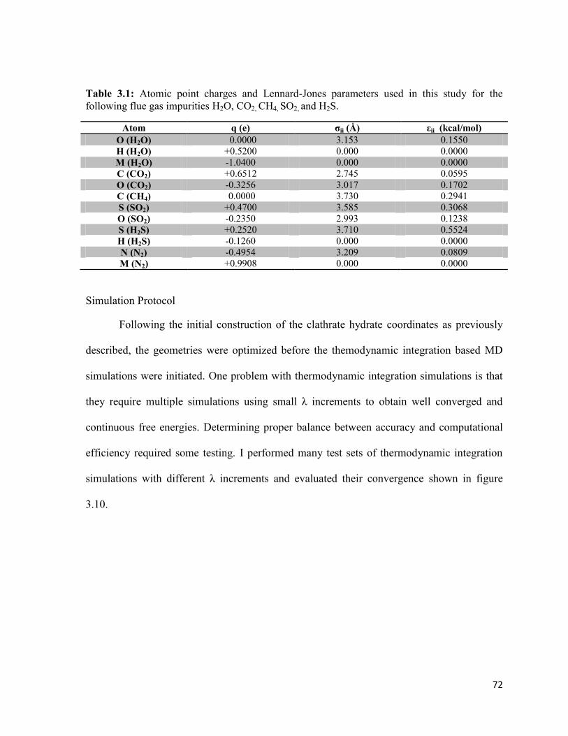
72
Table 3.1: Atomic point charges and Lennard-Jones parameters used in this study for the
following flue gas impurities H2O, CO2, CH4, SO2, and H2S.
Atom q (e) σii (Å) εii (kcal/mol)
O (H2O) 0.0000 3.153 0.1550
H (H2O) +0.5200 0.000 0.0000
M (H2O) -1.0400 0.000 0.0000
C (CO2) +0.6512 2.745 0.0595
O (CO2) -0.3256 3.017 0.1702
C (CH4) 0.0000 3.730 0.2941
S (SO2) +0.4700 3.585 0.3068
O (SO2) -0.2350 2.993 0.1238
S (H2S) +0.2520 3.710 0.5524
H (H2S) -0.1260 0.000 0.0000
N (N2) -0.4954 3.209 0.0809
M (N2) +0.9908 0.000 0.0000
Simulation Protocol
Following the initial construction of the clathrate hydrate coordinates as previously
described, the geometries were optimized before the themodynamic integration based MD
simulations were initiated. One problem with thermodynamic integration simulations is that
they require multiple simulations using small λ increments to obtain well converged and
continuous free energies. Determining proper balance between accuracy and computational
efficiency required some testing. I performed many test sets of thermodynamic integration
simulations with different λ increments and evaluated their convergence shown in figure
3.10.

73
Figure 3.10: Plot representing the free energy convergence of the error function as a
function of the λ increment (number of simulations). It is clear that the free energy converges
at λ 0.05
It can be observed that the Gibbs free energy can be determined with sufficient
accuracy with a λ increment of 0.05. Therefore, 21 total simulations where ideal to perform
the transformation of the CO2 in the clathrate hydrate phase to guest Y (i.e. methane,
nitrogen, hydrogen sulfide and sulfur dioxide). In the product CO2(g), molecules are
randomly replaced from both small and large cages with Y guests. Recall, to transform a
reactant to a product the λ parameter must be applied to the potential energy functions
describing the intermolecular interactions. The replacement fractions of the CO2(g) guests in
the small and large cages in the simulation cell can vary from λ = 0.0 to 1.0 in intervals of
0.05, thus leading to a total of 21 simulations to complete the transformation. Additionally,
large cage and small cage substitutions were also performed separately allowing us to further
understand the driving force behind the substitutions. Finally, the same procedure was
implemented to determine the separate contributions of the Van der Waals and electrostatic
-3000
-2000
-1000
0
1000
2000
3000
4000
5000
0 0.2 0.4 0.6 0.8 1
λ
λ sensitivity test using the non-linear Error Function
lambda 0.1
lambda 0.05
lambda 0.025
λ increment
(kc
al/m
ol)

74
parts of the intermolecular potential energy to the total Gibbs free energy of CO2
substitution.
The thermodynamic integration method may seem tedious because there are a total of
4 different guests (i.e. CH4, SO2, H2S, and N2) and total of 5 different types of
transformations for each guest (full cage substitution at 200 K, full cage substitution at 273
K, large cage substitution, small cage substitution and partial non-bonded substitution) all
requiring 21 simulations to complete the transformation (420 total simulations). However,
this work was feasible as I developed a Python program to automate the process for creating
appropriate simulations for thermodynamic integration techniques. The program requires
minimal supplementary input from the user to generate simulations suitable for free energy
calculations using thermodynamic integration based on typical classical molecular dynamics
inputs. In general, only three inputs are required for typical DL_POLY simulations; 1) The
CONFIG file which contains all the coordinates for the atoms in the system, 2) The FIELD
file which contains the force field parameters and 3) the CONTROL file which contains all
the simulation parameters and specifications such as temperature, pressure, simulation time
etc… The latter files all need to be altered when performing free energy calculations based
on thermodynamic integration. My program can perform these changes and submit these
simulations using the DL_POLY 2.20 molecular dynamics package with nothing more than
the coordinates and atomic types of the Y guest molecule of interest. The program begins by
randomly selecting CO2 molecules located in the CONFIG file in the desired category (all
cages, large cages, and small cages) for transformation. The program then creates the
coordinates for the Y guests in the appropriate Cartesian space (Y guest is created near the

75
randomly selected CO2 guest) and generates the appropriate CONFIG file necessary for free
energy calculations based on thermodynamic integration. The program then uses the atomic
types provided by the user and a tabulated list of potentials to determine the non-bonded
potentials describing the interactions of the newly added Y guest with all of the existing
atoms in the simulation calculated using typical Lorentz-Bertholet combination rules:
( )
3.25
( ) ⁄ 3.26
Where the indices and represent all the atoms involved in the pairwise interactions,
represents the well depth of the potential energy describing the Van der Waals interactions at
equilibrium, represents the finite distance between the pairwise interactions for all atoms
where the Van der Waals interaction energy is zero. The program then generates the
necessary FIELD file suitable for free energy simulations based on thermodynamic
integration. Finally, the program also modifies the CONTROL file appropriately. More
specifically, the program analyzes the previously created input files and generates a new
CONTROL file with the necessary free energy initiation specifications such as the reactant
and product atoms, lambda value and other parameters necessary for proper thermodynamic
integration procedure. Once all the newly created input files are complete, they are submitted
with the lambda value 0 to 1 in increments of 0.05 creating the aforementioned 21
simulations required to complete a transformation. These simulations can all run
simultaneously.
Simulations were all performed using the DL_POLY 2.20 molecular dynamics
program34
in the NpT ensemble with Nosé/Hoover thermostat and barostat constants of 0.2

76
and 0.5 ps, respectively. The temperature and pressure of the simulations were 200 K and 1
bar. In addition, simulations were also performed at 273 K to observe the effect of
temperature on the free energy of substitution. Simulations were carried out for 500 ps with
the first 100 ps used for equilibration with a timestep of 1 fs to integrate the equations of
motion. All simulations used the SHAKE algorithm for rigid molecule motion. The Ewald
summation method was used to treat Coulombic interactions and all intermolecular
interactions in the simulation box were calculated within a cutoff distance of 13 Å.

77
Results and Discussion
Structure I clathrate hydrates have been suggested as carbon dioxide
capture/separation tools for flue stream derived from coal combustion plants. Understanding
the disruption potential of common gas impurities found in the flue stream at conditions
relevant for hydrate formation (273 K and 10 bar) is imperative for determining the
feasibility of this method. Our goal is to evaluate the relative thermodynamic stability of
each sI clathrate hydrate (i.e. CH4, CO2, N2, SO2, and H2S) using Gibbs free energy
calculations based on thermodynamic integration via MD simulations. These substitution
thermodynamics will be evaluated for three different substitutions: the full substitutions in all
cages, the substitutions in the large cages only and finally the substitution in the small cages
only. The effect of temperature on the substitution process will also be investigated. Finally,
by partitioning the non-bonded potential into separate contributions (i.e. Van der Waals and
electrostatics) we hope to acquire further insight on the driving force behind the substitution
process.
Recall, there are two components to the substitution process, the guest substitution in
the clathrate phase (calculated from simulation) and the guest substitution in the gas phase
(calculated using the non-ideality component). Simulations provide the free energy for the
guest substitution in the clathrate phase. These simulations were performed at a temperature
of 273 K and 1 bar of pressure. Since the clathrate is non-compressible, this is a good
approximation for conditions relevant for hydrate formation (10 bar). An example of the
integrand in equation 3.8 is shown in figure 3.11 where all CO2 guests in the sI clathrate are
replaced by SO2 guests (substitution in equation 3.33).

78
Figure 3.11: A representation of the ⟨ ( )
⁄ ⟩
for different values of λ for the CO2→SO2
substitution in the clathrate hydrate. The integration of this curve gives ΔGTI.
Initially, at λ=0 the Gibbs free energy is positive thus unfavorable (CO2-cage
interactions are dominant). As λ varies from 0 to 0.5 (weakening of the CO2–cage
interactions and strengthening the SO2–cage interactions), the free energy change tends to
more negative values. This suggests that the SO2-cage interactions are more favorable than
the CO2-cage interactions. Moreover, once λ>0.5, the Gibbs free energy change becomes
favorable, this is a result of the SO2-cage interactions becoming more dominant than the less
favored CO2-cage interactions. Evaluating the area under the curve in figure 3.11 provides
ΔGTI for the substitution in equation 3.31.
`
⟨ ( )
⟩
(kcal/mol)

79
a. CO2 substitution with CH4
The Gibbs free energy of the carbon dioxide guest substitutions with methane in the
sI clathrate hydrate cages are given in table 3.2. In the first set of simulations, all CO2 guests
in the sI clathrate hydrate are substituted by CH4 guests at 273 K and 10 bar (equation 3.27).
[ ( )] ( ) [ ( )] ( ) 3.27
Table 3.2: Gibbs free energy per guest substitution of CO2(clathrate) → CH4(clathrate) in
the sI clathrate hydrate at 273 K 10 bar. The Non-ideal gas contributions are calculated at
conditions relevant for hydrate formation (273 K and 10 bar). Van der Waals and
electrostatic contributions to the total Gibbs free energy are also presented.
Substitution ΔGTOT
(kcal/mol)
ΔGTI
(kcal/mol)
ΔGNon-ideality
(kcal/mol)
ΔGTI (VdW)
(kcal/mol)
ΔGTI (Elec.)
(kcal/mol)
All cages -0.39 -0.38 -7.1×10⁻³
-0.38 -
Large cages - -0.39 - - -
Small cages - -1.54 - - -
The total Gibbs free energy for the substitution in equation 3.27 is –0.39 kcal/mol for
each guest. This value includes the non-ideality effects of the molecule exchange in the gas
phase (-7.1x10⁻³
kcal/mol). These results demonstrate that methane sI clathrate hydrates are
more stable than CO2 sI clathrate hydrates at 273 K and 10 bar. Further dissection of the free
energy reveals the separate contributions of the small and large cages. The Gibbs free energy
for the substitution of CO2 with CH4 in the large cages only (equation 3.28) is -0.39 kcal/mol
per guest.
[ ( )] ( ) [ ( ) ( )] ( ) 3.28

80
Furthermore, the substitution of CO2 with methane in the small cages only (equation 3.29) is
–1.54 kcal/mol per guest.
[ ( )] ( ) [ ( ) ( )] ( ) 3.29
These values show that the carbon dioxide gas in both the large and small cages of
CO2 sI clathrate hydrates are thermodynamically susceptible to substitution with CH4.
Unfortunately, these favorable Gibbs free energy differences suggest that if a significant
amount of uncombusted methane is present in the flue stream, it may spontaneously replace
CO2 in both the small and large cages. Although the bulk of the CO2 capacity (large cages)
will remain unsubstituted the 2:6 small cage/large cage ratio of sI clathrate hydrate indicates
that methane can considerably impede efficient carbon capture. This suggests that CO2
capture using sI clathrate hydrates will not likely be feasible at 273 K and 10 bar.
In addition, partitioning the cage substitutions into large and small cages allow us to
evaluate the effect of binary hydrates. These effects will demonstrate the influence of a
binary CO2/CH4 sI clathrate hydrate on the thermodynamics stability of CO2CH4
substitutions. Table 3.2 summarizes our results. Results in table 3.2 suggest that the most
stable phase of the sI clathrate hydrate occurs when the small cages are substituted with
methane and the large cages are occupied by CO2 (largely negative ∆G for small cage
substitutions). These small cage substitutions are ideal in terms of using binary clathrates as
hydrate promoters, as they will not hinder the bulk of the CO2 uptake capacity. Promoters are
suggested for reducing the conditions (temperature and pressure) necessary to form the
hydrates. However, the large cage substitution can also be favored; this is problematic in the
carbon capture application because the large cages represent the bulk to the CO2 uptake

81
capacity. Thus its consideration as a hydrate promoter at these conditions (273 K and 10 bar)
should be questioned.
The united atom TRAPPE potential was chosen to represent CH4. Our simulations
were able to study the separate contributions of the Van der Waals and the electrostatics to
the Gibbs free energy of substitutions. This methane potential would suggest that the
favourability of the CO2CH4 substitutions is related to the effective radius of methane.
Table 3.6 demonstrates that the Van der Waals radius of methane is much smaller than that
of CO2, this can make it easier to accommodate in the cages resulting in a favorable ΔGVDW
(negative ΔGVDW given in table 3.2). However, further dissection of the separate
contributions is not possible as this model does not utilize charges to describe methane
behavior. Instead, it uses only the Van der Waals interactions to represent methane
interactions. In order to make any conclusions, the effect of the non-bonded potential of
methane on the ∆GTOT should be investigated.
b. CO2 substitution with N2
The Gibbs free energy of the carbon dioxide guest substitutions with nitrogen in the
sI clathrate hydrate cages are given in table 3.3. In the first set of simulations, all CO2 guests
in the sI clathrate hydrate are substituted by N2 guests at 273 K and 10 bar (equation 3.30).
[ ( )] ( ) [ ( )] ( ) 3.30

82
Table 3.3: Gibbs free energy per guest substitution of CO2(clathrate) → N2(clathrate) in the
sI clathrate hydrate at 273 K 10 bar. The Non-ideal gas contributions are calculated at
conditions relevant for hydrate formation (273 K and 10 bar). Van der Waals and
electrostatic contributions to the total Gibbs free energy are also presented.
Substitution ΔGTOT
(kcal/mol)
ΔGTI
(kcal/mol)
ΔGNon-ideality
(kcal/mol)
ΔGTI (VdW)
(kcal/mol)
ΔGTI (Elec.)
(kcal/mol)
All cages 1.37 1.36 -9.7×10⁻³
0.33 1.03
Large cages - 1.59 - - -
Small cages - -0.20 - - -
The total Gibbs free energy for the substitution in equation 3.30 is 1.37 kcal/mol for
each guest. This value includes the non-ideality effects of the molecule exchange in the gas
phase (-9.7x10⁻³
kcal/mol). These results demonstrate that carbon dioxide sI clathrate
hydrates are more stable than nitrogen sI clathrate hydrates. This behavior is to be expected,
as sI nitrogen clathrate hydrates do not form at conditions of 273 K and 10 atm. As a result
this gas cannot be considered as a hydrate promoter. Further dissection of the free energy
reveals the separate contributions of the small and large cages. The Gibbs free energy for the
substitution of CO2 with N2 in the large cages only (equation 3.31) is 1.59 kcal/mol per
guest.
[ ( )] ( ) [ ( ) ( )] ( ) 3.31
Additionally, the substitution of CO2 with N2 in the small cages only (equation 3.32) is –0.20
kcal/mol per guest.
[ ( )] ( ) [ ( ) ( )] ( ) 3.32
These values show that the carbon dioxide gas in the large cages of CO2 sI clathrate
hydrates are not thermodynamically susceptible to substitution with N2. However, the Gibbs
free energy for the substitution of carbon dioxide gas in the small cages of CO2 sI clathrate

83
hydrates show that CO2 in the small cages are thermodynamically susceptible to substitution
with N2. These results indicate that the most stable form of the sI clathrate hydrate would be
a binary CO2/N2 hydrate phase, where CO2 is in the large cages and N2 in the small cages.
Unfortunately, due to the high concentration of nitrogen in the atmosphere and in the
combustion gas, CO2 capture using sI clathrate hydrates could be severely hampered by the
formation of N2 clathrates at 273 K and 10 bar. Although the bulk of the cages (large cages)
in CO2 sI clathrate hydrates are not susceptible to substitution with N2, the small cages of
CO2 sI clathrate hydrates can be substituted. Since the small cage/large cage ratio of sI
clathrate hydrate is 2:6, this suggests that 25% of the CO2 capacity can be substituted
resulting in a drastic decrease in carbon capture efficiency. As a result, sI clathrate hydrates
could consume large amounts of energy to capture N2 (a harmless gas) from flue stacks. This
could have serious implications for CO2 capture by clathrate hydrates. It is important to note
that these simulations only investigate the thermodynamics of substitution. Kinetics of N2
substitution in the small cages of sI clathrate hydrate is also important.
Separate contributions of the N2 non-bonded potential were also analyzed in hopes of
gaining a better understanding of the small vs large cage selectivity. These values are given
in table 3.3 and show that the electrostatic contribution to the ΔGTI is larger than the Van der
Waals contribution (1.03 and 0.33 kcal/mol, respectively). From the values given in table
3.6, we can see that the Van der Waals radius of N2 is significantly smaller than CO2. This
would make this guest easier to accommodate in the small sI clathrate hydrate cages. This
should result in a smaller contribution of the ΔGVdW to the positive ΔGTI (shown in table 3.3).
Furthermore, the large positive ∆GElec. suggests that N2 is disfavored in the large cages due to

84
its electrostatics. This could be a result of the smaller quadrupole moment of N2 compared to
the larger more favorable quadrupole moment of CO2. The effect of multipole moments
should be further investigated before determining the fundamental reason for selectivity.
Table 3.4: The molar volumes of CO2, CH4, and N2 (m3/mol) at 200 K for different
pressures (bar) and the residual contribution to the Gibbs free energy from each gas
(kcal/mol). d
at 273 K
Gas Pressure
(bar)
Vm(p,T)
(m3/mol)
),( TpV ig
m
(m3/mol)
TpVTpV ig
mm ,,
(m3/mol)
)],;(X[ pTgres
CO245
0.5 0.032940 0.033260 -3.2×10⁻⁴
1 0.016312 0.016628 -3.2×10⁻⁴
-2.40×10⁻⁴
1.01325 0.016094 0.016411 -3.2×10⁻⁴
10 f 0.002081 0.002245 -1.6×10
-4 -1.55×10
-4
CH446
0.1 0.16617 0.16628 -1.1×10⁻⁴
0.5 0.033156 0.033256 -1.0×10⁻⁴
1 0.016523 0.016628 -1.0×10⁻⁴
-1.04×10⁻⁴
1.01325
0.016305 0.016411 -1.0×10⁻⁴
10 d 0.002189 0.002245 -5.5×10
-5 -5.53×10
-4
N247
0.2 0.083126 0.083145 -1.9×10⁻⁵
0.4 0.041528 0.041572 -4.4×10⁻⁵
0.6 0.027678 0.027715 -3.7×10⁻⁵
0.8
0.0207512 0.020786 -3.5×10⁻⁵
1 0.016593 0.016629 -3.6×10⁻⁵
-3.11×10⁻⁵
1.01325 0.016375 0.016411 -3.7×10⁻⁵
10 d 0.002234 0.002245 -1.1×10
-5 -1.09×10
-4

85
Table 3.5: Simulation cell volumes (Å3) for each clathrate at 200K and 1 bar.
V(clathrate; T,p)
),;(
),;(ln
2CO
Y
pTclathrate
pTclathrate
Clathrate(CO2) 44877 -
Clathrate(SO2) 45475 -0.013
Clathrate(H2S) 44376 0.011
Clathrate(CH4) 44671 0.005
Clathrate(N2) 44581 -0.007
Table 3.6: The van der Waals radii (Å) and polarity of the guest species Y studied in this work.
Y van der Waals radius (Å) a Electrostatic moment
SO2 3.98 μ = 1.62 D b
CO2 3.85 Θ = –4.3×10⁻²⁶
statC·cm2 c
H2S 3.12 μ = 0.97 D d
CH4 2.98 N/A e
N2 2.65 Θ = –1.4×10⁻²⁶
statC·cm2 c
a Ref.
48,49
b Ref.
39
c Ref.
50
d Ref.
40
e No electrostatic charge is used in the united atom TRAPPE potential for CH4.
c. CO2 substitution with SO2
The Gibbs free energy of the carbon dioxide guest substitutions with sulfur dioxide in
the sI clathrate hydrate cages are given in table 3.7. Unfortunately, the necessary
thermophysical data for SO2 (and H2S) is not available to calculate the ∆Gnon-ideal component
of the ∆GTOT in the same manner as was determined for CH4 and N2 using the first and
second term in equation 3.18 and the data presented in tables 3.4 and 3.5. However, at these
pressures (10 bar) we note that these non-ideal corrections for nitrogen and methane are on
the orders of 10-3
kcal/mol and account for less than 2% of the ∆GTOT (refer to table 3.2 and
3.3). Therefore, ∆Gnon-ideal is approximated to be zero in the calculation of the ∆GTOT for SO2
and H2S. This approximation can be further justified by considering the gases as ideal

86
(equation 3.19 and 3.20) and by considering the clathrate hydrates as non-compressible
(equation 3.21).
In the first set of simulations, all CO2 guests in the sI clathrate hydrate are substituted
by SO2 guests at 273 K and 10 bar (equation 3.33).
[ ( )] ( ) [ ( )] ( ) 3.33
Table 3.7: Gibbs free energy per guest substitution of CO2(clathrate) → SO2(clathrate) in the
sI clathrate hydrate at 273 K 10 bar. Van der Waals and electrostatic contributions to the total
Gibbs free energy are also presented.
Substitution ΔGTOT
(kcal/mol)
ΔGTI (VdW)
(kcal/mol)
ΔGTI (Elec.)
(kcal/mol)
All cages -1.63 -0.99 -0.91
Large cages -2.05 - -
Small cages -0.63 - -
The total Gibbs free energy for the substitution in equation 3.33 is –1.63 kcal/mol for
each guest. These results demonstrate that SO2 sI clathrate hydrates are more stable than
CO2 sI clathrate hydrates. Further examination of the free energy reveals the separate
contributions of the small and large cages. The Gibbs free energy for the substitution of CO2
with SO2 in the large cages only (equation 3.34) is -2.05 kcal/mol per guest.
[ ( )] ( ) [ ( ) ( )] ( ) 3.34
The substitution of CO2 with SO2 in the small cages only (equation 3.35) is –0.63 kcal/mol
per guest.
[ ( )] ( ) [ ( ) ( )] ( ) 3.35

87
These values show that the carbon dioxide gas in both the large and small cages of
CO2 sI clathrate hydrates are thermodynamically susceptible to substitution with sulfur
dioxide. Furthermore, these favorable Gibbs free energy differences suggest that if SO2 is
present in sufficient quantities in the flue stream, CO2 capture using sI clathrate hydrates may
not be feasible at 273 K and 10 bar. Fortunately, current desulfurization technologies are
very mature and wide spread.54
CO2/SO2 binary sI clathrate hydrates were also studied. These effects are shown in
table 3.7. When evaluating the Gibbs free energy for substituting the large cages only
(equation 3.34), it is clear that having a binary CO2/SO2 sI clathrate hydrate, with CO2 is in
the small cages and SO2 in the large cages will be the most stable phase for this hydrate.
This computational prediction is in agreement with experimental studies which show that the
phase boundary for the CO2/SO2 binary sI clathrate hydrate is found at lower pressures and
temperatures compared to the CO2 sI hydrate (refer to figure 3.4).18,51
Unfortunately, this gas
favors the large cages and forms clathrates more readily than CO2, thus this gas should not be
investigated as a hydrate promoter, as it will impede the bulk of the CO2 capture. Therefore,
this impurity would need to be removed further from the flue stream prior to CO2 capture.
The contribution of the Van der Waals and electrostatic potentials to the Gibbs free
energy for the CO2SO2 transformation are shown in table 3.7. These values are almost
equal at –0.99 and –0.91 kcal/mol, respectively. Both contributions have a negative Gibbs
free energy implying that SO2 is the thermodynamically favored guests over CO2 from both
the van der Waals guest – water and electrostatic guest-water interactions. Let us examine

88
the van der Waals radius and electrostatic moment of SO2 given in table 3.6 to further
understand SO2 selectivity.39,40,48-50,52
Van der Waals radii values show that SO2 is larger
than CO2, therefore there must be another underlying reason that SO2 is favored in both
small and large cages in terms of ∆GVdW. Table 3.6 also demonstrates the electrostatic
moment of SO2 is considerably larger than any other guests. However, further investigation
is required to understand the favorable nature of the ∆GVdW and ∆GElec. before the underlying
reason can be conclusively determined.
d. CO2 substitution with H2S
The Gibbs free energy of the carbon dioxide guest substitutions with hydrogen
sulfide in the sI clathrate hydrate cages are given in table 3.8. In the first set of simulations,
all CO2 guests in the sI clathrate hydrate are substituted by H2S guests at 273 K and 10 bar
(equation 3.36).
[ ( )] ( ) [ ( )] ( ) 3.36
Table 3.8: Gibbs free energy per guest substitution of CO2(clathrate) → H2S(clathrate) in the
sI clathrate hydrate at 273 K 10 bar. Van der Waals and electrostatic contributions to the total
Gibbs free energy are also presented.
Substitution ΔGTOT
(kcal/mol)
ΔGTI (VdW)
(kcal/mol)
ΔGTI (Elec.)
(kcal/mol)
All cages -1.55 -1.30 -0.26
Large cages -1.12 - -
Small cages -2.73 - -
The total Gibbs free energy for the substitution in equation 3.36 is –1.55 kcal/mol for
each guest. These results demonstrate that H2S sI clathrate hydrates are more stable than CO2
sI clathrate hydrates. Further dissection of the free energy reveals the separate contributions

89
of the small and large cages. The Gibbs free energy for the substitution of CO2 with H2S in
the large cages only (equation 3.37) is -1.12 kcal/mol per guest.
[ ( )] ( ) [ ( ) ( )] ( ) 3.37
Furthermore, the substitution of CO2 with SO2 in the small cages only (equation 3.37) is
–2.73 kcal/mol per guest.
[ ( )] ( ) [ ( ) ( )] ( ) 3.38
These values show that the carbon dioxide gas in both the large and small cages of
CO2 sI clathrate hydrates are thermodynamically susceptible to substitution with hydrogen
sulfide. Unfortunately, these favorable Gibbs free energy differences suggest that if H2S is
present in the flue stream, CO2 capture using sI clathrate hydrates will not likely be feasible
at 273 K and 10 bar. Similar to the case of SO2, if H2S is present in sufficient quantities it can
considerably impede efficient carbon dioxide capture. Fortunately, due to the toxicity of
hydrogen sulfide and its high concentration in “sour gas”, combustion plants today are
equipped with technologies for removing this contaminant before it is released into the
atmosphere.54
CO2/H2S binary sI clathrate hydrates were also studied. These effects are shown in
table 3.8. Contrary to SO2, the free energy values presented in table 3.8 suggest that a binary
CO2/H2S sI clathrate hydrate, with CO2 is in the large cages and H2S in the small cages will
be the most stable phase for this hydrate. Unlike SO2, little is known of the clathrate hydrate
formation potential of H2S and further investigation of this gas’ clathrate hydrate formation
potential is necessary before conclusion can be made on the its efficacy to hinder clathrate

90
hydrate CO2 uptake.53
If the hydrate formation potential of H2S coincides with the conditions
necessary for carbon capture using clathrate hydrates, it too could have the capability of
obstructing CO2 capture. This would result in the necessary removal of the H2S impurity
from the flue stream prior to CO2 capture. However, as previously mentioned the most stable
phase for these clathrates contain CO2 in the large cages and H2S in the small cages. This
type of binary hydrate is an ideal candidate in the hydrate promotion application. If hydrogen
sulfide clathrates require milder conditions, the possibility of using this gas as a promoter
exists. Unfortunately, large cage substitutions are also still favored this will likely further
discredit the use of sI clathate hydrates as carbon capture tools.
Similarly, Van der Waals and electrostatic contributions to the ΔGTI were evaluated.
According to the results in table 3.8 the ∆GVdW is much larger than the electrostatic
contribution (–1.30 and –0.26 kcal/mol per guest, respectively). Referring to table 3.6, we
can observe that the Van der Waals radius of H2S is significantly smaller than CO2 which
makes it easier to accommodate into the sI clathrate hydrate cages. This could account for
the Van der Waals stabilization effect to the Gibbs free energy. Furthermore, the smaller
magnitude of the dipole moment of the H2S guests compared to SO2 can be attributed to the
smaller magnitude of the electrostatic contributions for ΔGTI for this guest. Nonetheless, the
small dipole moment of H2S leads to favorable contributions of the electrostatic potential to
free energies of substitution of CO2. The effects of the separate components of the non-
bonded potential should be further investigated before determining the fundamental reasons
for selectivity.

91
e. Effect of temperature on the Gibbs free energy of substitution
Since the free energies of substitution evaluated at 273 K do not bode well for CO2
capture with clathrate hydrates, we examined the free energies of substitution at a lower
temperature (200K). This should give us some indication of the effect of temperature on the
Gibbs free energy for CO2 substitutions with flue gas impurities. Our results are summarized
in table 3.9.
Table 3.9: Gibbs free energy per guest substitution of CO2(clathrate) → Y(clathrate) in the
sI clathrate hydrate at 273 K and 200 K at 10 bar.
Y Substitution ΔGTOT
(273 K)
kcal/mol
ΔGTOT
(200 K)
kcal/mol
SO2 All cages -1.63 -1.90
Large cages -2.05 -2.30
Small cages -0.63 -0.77
CH4 All cages -0.38 -0.13
Large cages -0.39 0.35
Small cages -1.54 -1.26
H2S All cages -1.55 -1.56
Large cages -1.12 -0.82
Small cages -2.73 -2.76
N2 All cages 1.11 1.36
Large cages 1.53 1.59
Small cages -0.20 -0.37
In all simulations with SO2, H2S, and N2, the value of the ΔGTI per guest molecule at
200 K varied by less than 0.3 kcal/mol per substitution relative to the values at 273 K. The
SO2 and H2S hydrates become slightly more thermodynamically stable at the 200 K relative
to CO2 clathrates in all substitution reactions, with the exception of the H2S large cage
substitutions. Unfortunately, the effect of temperature in these cases further hinders the CO2
uptake and the feasibility of using sI clathrate hydrates as carbon capture tools. On the other
hand, N2 substitutions are only further stabilized in the small cages; otherwise the

92
substitutions in the large cages are further destabilized. It is clear that the effect of
temperature does not change the thermodynamics of substitution for SO2, H2S and N2 in
terms of CCS application. However, in the case of CH4 hydrates the substitution
thermodynamics in the large cages become significantly less stable at 200 K. We can observe
this by comparing the Gibbs free energy difference at 273 K and 200K (-0.39 kcal/mol per
guest vs 0.35 kcal/mol per guest, respectively). This makes the CO2 guests in the large cages
of sI clathrate hydrate unsusceptible to substitutions. Consequently, the decrease in
temperature can have a profound impact on the feasibility of using sI hydrates for carbon
capture. Because CH4 is favored only in the small cages, it has potential to be used as a
hydrate promoter. Meaning it may be able to reduce the conditions of hydrate formation,
making it easier to form CO2 clathrates in a binary CO2/CH4 mixture. Furthermore, the large
cage substitutions are now disfavored, this renders in the bulk of the CO2 capacity (large
cages) unsusceptible to substitutions. These nonspontaneous substitutions make binary
CO2/CH4 hydrates prime candidates for hydrate promotion. Additionally, because CH4
favors the replacement of CO2 in the small cages, it will have minimal impact on the CO2
uptake capacity of the hydrate (2:6 small cage/large cage ratio). However, uncombusted
methane is not very concentrated in the flue stream, thus the use of CH4 as a promoter should
be investigated further to determine if the reduction of the conditions (temperature and
pressure) for hydrate formation outweighs the compromise in CO2 uptake capacity. These
studies would indicate that having a binary CO2/CH4 hydrate would be economically feasible
compared to the pure CO2 hydrates. Furthermore, substituting CO2 in the small cages may
not have a negative effect in terms of capture. Since CH4 is a much more potent (21 times)
greenhouse gas than CO2, it is also desirable to remove this flue gas impurity from the

93
atmosphere. The binary CO2/CH4 hydrates should be further investigated in the application
of carbon capture.
Results from a previous study by the Woo Lab on methane substitution with CO2
from the sI clathrate hydrate under deep ocean pressures and temperatures near 273 K,27
are
in agreement with this work. The Woo lab found that CO2 is favored in the large sI cages,
and CH4 is favored in the small sI clathrate hydrate cages. The relative magnitude of the
Gibbs free energy for substitution of CO2 with CH4 in the small and large cages is different
in this work and Ref. [27] and this can be related to the different thermodynamic conditions
of the two sets of simulations or the different intermolecular potential used for methane in
Ref. [27]. Although the results are considerably different, the same trends can be drawn and
used to conclude that a binary mixture of CO2/CH4 is the most stable clathrate hydrate that
can form at the given temperatures and conditions.
Another previous study performed by the Woo lab was used to determine the
methane storage capacity in the structure H clathrate hydrate under high pressure
conditions.30,31
In those studies, it was observed that the calculated values of the Gibbs free
energy for methane encapsulation from the gas phase show strong sensitivity to the
intermolecular potential energy function used for methane. This must be taken into account
when interpreting the numerical values of the Gibbs free energy of CO2 substitution with
CH4.
94
Conclusions
Molecular dynamics simulations were used to evaluate the free energy of substituting
CO2 in clathrate hydrates by N2,CH4, SO2 and H2S flue gas impurities under conditions
proposed for CO2 capture (273 K, 10 bar). Under these conditions, structure I CO2 clathrate
hydrates that have both small and large cages in a 2:6 ratio are known to form. In this work,
our goal was to examine how thermodynamically susceptible CO2 sI clathrates were to
substitution by N2,CH4, SO2 and H2S in both the large and small cages.
For post-combustion CO2 capture, nitrogen is an important gas to consider for
substitution as it is present in high concentrations within the combustion flue gas. Although
N2 clathrate hydrates do not form at these temperature and pressure conditions, our
simulations suggested that CO2 sI clathrates may be susceptible to substitution by N2 only in
the small cages. More specifically, we found that CO2 substitution by N2 in the small sI
cages was thermodynamically favorable by 0.20 kcal/mol per guest substitution. This
substitution is problematic in terms of efficient CO2 capture because a significant amount of
energy is spent on forming the N2 clathrates. Since the small cages make up 25% of the sI
clathrate cages, a significant amount of energy could be spent on removing N2 from the flue
gas rather than CO2. It is important to note that these simulations only evaluate the
thermodynamics of the substitution process, not the kinetics of the process. So if the
substitution is slow, the presence of N2 may not be problematic for CO2 capture using
clathrate hydrates. Unfortunately, previous experimental studies of methane clathrates under
similar conditions (Park et al. Proc. Natl. Acad. Sci. U.S.A. 2006, 103, 12690) revealed that
N2 can rapidly substitute CH4 in the sI clathrates. The kinetics of CO2 sI calthrate
substitution by N2 is not expected to be significantly different, however further experimental
study of this issue is necessary to confirm this assertion.

95
The thermodynamics of CO2 substitution by SO2 and H2S in sI clathrate hydrates was
also examined. In both cases, the substitution was highly favored in the full cage substitution
process (1.63 and 1.55 kcal/mol for SO2 and H2S, respectively). Moreover, substitution of
CO2 by these gases in both the small and large cages was determined to be favorable. This
suggests that these gases may also disrupt the CO2 capture by sI clathrate hydrates if they are
present in large concentrations in the combustion flue stream. However, since these gases are
not typically present in high concentration due to desulfurization technologies, they should
not present a problem for post-combustion CO2 scrubbing. Unfortunately, SO2 and H2S gases
can be present in relatively high concentration in natural gas from so-called unconventional
reservoirs (reservoirs not usually fit or selected for natural gas extraction due to their
contamination). Presently, there are increasing amounts of natural gases being extracted from
unconventional reservoirs such as shale gas due to the shortage of conventional (ideal)
reservoirs. As a result, there is an interest in CO2 scrubbing technologies for natural gas
purification. These reservoirs typically have high levels of CO2 (~15%), where clathrate
hydrates could be used for CO2 removal in pre-combustion purification. Since SO2 and H2S
need to be removed from natural gas, our results suggest that a sI clathrate hydrate based
technology (at conditions of 200K and 10 bar) could be used for removal of all three gases.
Finally, the thermodynamics of CO2 substitution by methane in sI clathrate hydrates
was examined. Substitution in both the small and large cages was calculated to be favorable,
although substitution in the small cages was significantly more exergonic with ∆GTOT being
-1.54 and -0.39 kcal/mol for small and large case substitutions, respectively. Since methane
is a 21 times stronger greenhouse gas than CO2, its concomitant removal during post-
combustion CO2 scrubbing is desirable. On the other hand, for natural gas purification, these

96
results suggest that a sI clathrate hydrate based technology could not be used since CO2
scrubbing would be disrupted by methane, the primary component of natural gas.
Because the results at 273 K and 10 bar were not particularly promising for CO2
capture by sI clathrate hydrates, we evaluated the same substitution thermodynamics at 200
K and 10 bar. This was done to determine if CO2 sI calthrate hydrates were less susceptible
to substitution at lower temperatures. With one exception, we found that the substitution free
energies change by less than 0.3 kcal/mol, and do not alter the sign of free energies. Thus,
using a lower capture temperature does not significantly change the substitution free energies
and their implications for CO2 capture by sI clathrate hydrates. The only exception to this
was the substitution of CO2 by CH4 in the large cages. The calculated substitution free
energy changed from ∆GTOT= -0.39 kcal/mol at 273 K to +0.35 kcal/mol at 200 K. This
might make it more feasible for using sI clathrate hydrates for natural gas purification,
however further analysis and experimentation would be required as lower temperature
processes are energetically costly.
The total free energies of substitution were also broken down into non-ideal gas
effects, Van der Waals and electrostatic contributions to the substitution process. At the
pressures proposed for CO2 capture (~10 bar) using sI clathrate hydrates, non-ideal gas
effects were found to be negligible and can be neglected for other gases under similar
conditions. The substitution free energies were also dissected into the individual
contributions of the non-bonded potential energy function (Van der Waals and electrostatics)
to evaluate their effect on the total Gibbs free energy of substitution between CO2 and flue
gas impurities in sI clathrate hydrates. It is clear that these contributing factors strongly

97
depend on the species of interest. However, it can be observed that the size of the guest plays
a major role in the substitution process. Further studies are required before accurate
conclusions can be made on the electrostatic contributions to the total Gibbs free energy of
substitution.
As part of this work, the free energy calculations were automated. In these
calculations, thermodynamic integration is performed where the CO2 molecules in the sI
clathrate hydrate cages are incrementally mutated into the substituting gases N2, SO2, H2S or
CH4. These simulations are tedious and are prone to human error because numerous steps are
involved in the setup of the molecular dynamics input files needed at each stage. Thus,
significant effort was put into fully automating the procedure, such that the user only needs
to create input files containing the atomic types and coordinates of the initial and final gases.
The program was capable of fully automating the procedure of creating all of the
intermediate input files, submitting the jobs, and integrating the free energy changes.
Moreover, the program was written in a way that it is not limited to the specific application
of clathrate hydrates. For example, it could be used to mutate a functional group within a
metal organic framework to examine the change in adsorption free energies. This will
greatly simplify and accelerate any future mutational free energy calculations done in the
Woo lab.

98
(1) Morgan, M. G.; Cantor, R.; Clark, W. C.; Fisher, A.; Jacoby, H. D.; Janetos,
A. C.; Kinzig, A. P.; Melillo, J.; Street, R. B.; Wilbanks, T. J. Environmental Science &
Technology 2005, 39, 9023-9032.
(2) Nations, U. http://www.ipcc.ch/SPM2feb07.pdf 2007.
(3) Nations, U. http://www.unfccc.int/resource/docs/convkp/conveng.pdf 1992.
(4) Nations, U. http://www.unfccc.int/resource/docs/convkp/kpeng.pdf 1998.
(5) Aaron, D.; Tsouris, C. Separation Science and Technology 2005, 40, 321-348.
(6) Klara, S. M.; Srivastava, R. D. Environmental Progress 2002, 21, 247-253.
(7) Oi, L. E. SIMS2007 Conference 2007, Telemark Univeristy College.
(8) Herzog, H. M., J.; Hatton, A. Clean air task force 2009.
(9) Banerjee, R.; Phan, A.; Wang, B.; Knobler, C.; Furukawa, H.; O'Keeffe, M.;
Yaghi, O. M. Science 2008, 319, 939-943.
(10) Vaidhyanathan, R.; Iremonger, S. S.; Shimizu, G. K. H.; Boyd, P. G.; Alavi,
S.; Woo, T. K. Science 2010, 330, 650-653.
(11) Haines, J.; Cambon, O.; Levelut, C.; Santoro, M.; Gorelli, F.; Garbarino, G.
Journal of the American Chemical Society 2010, 132, 8860-+.
(12) Han, S. S.; Choi, S. H.; van Duin, A. C. T. Chemical Communications 2010,
46, 5713-5715.
(13) Adeyemo, A.; Kumar, R.; Linga, P.; Ripmeester, J.; Englezos, P.
International Journal of Greenhouse Gas Control 2010, 4, 478-485.
(14) Linga, P.; Kumar, R.; Lee, J. D.; Ripmeester, J.; Englezos, P. International
Journal of Greenhouse Gas Control 2010, 4, 630-637.
(15) Sloan, E. D. Journal of Chemical Thermodynamics 2003, 35, 41-53.
(16) Petrucci, R. H. H., F.G.; Madura, J.D.; Bissonnette, C. Pearson 2011, 10,
214,560.
(17) Linga, P.; Kumar, R.; Englezos, P. Journal of Hazardous Materials 2007,
149, 625-629.
(18) Beeskow-Strauch, B.; Schicks, J. M.; Spangenberg, E.; Erzinger, J.
Chemistry-a European Journal 2011, 17, 4376-4384.

99
(19) Stevens, S. H.; Kuuskraa, V. A.; Gale, J. In Greenhouse Gas Control
Technologies; C S I R O: East Melbourne, 2001, p 278-283.
(20) Stevens, S. H. K., V. A.; Gale, J.; Beecy, D. Envir. Geosciences 2001, 8, 200-
209.
(21) House, K. Z.; Schrag, D. P.; Harvey, C. F.; Lackner, K. S. Proceedings of the
National Academy of Sciences of the United States of America 2006, 103, 12291-12295.
(22) Côté, M. M. W., J. F. SPE, DOI: 10.2118/138121-MS.
(23) Uddin, M.; Coombe, D.; Law, D.; Gunter, B. Journal of Energy Resources
Technology-Transactions of the Asme 2008, 130, 14.
(24) Uddin, M.; Coombe, D.; Wright, F. Journal of Energy Resources Technology-
Transactions of the Asme 2008, 130, 11.
(25) Wright, J. F. C., M. M.; Dallimore S. R. Proced. 6th Inter. Conf. Gas
Hydrates 2008, Vancouver, BC, Canada.
(26) Englezos, P. Industrial & Engineering Chemistry Research 1993, 32, 1251-
1274.
(27) Dornan, P.; Alavi, S.; Woo, T. K. Journal of Chemical Physics 2007, 127, 8.
(28) Susilo, R.; Alavi, S.; Ripmeester, J.; Englezos, P. Fluid Phase Equilibria
2008, 263, 6-17.
(29) Alavi, S.; Ripmeester, J. A.; Klug, D. D. Journal of Chemical Physics 2006,
125, 10.
(30) Alavi, S.; Ripmeester, J. A.; Klug, D. D. Journal of Chemical Physics 2007,
126, 6.
(31) Alavi, S.; Woo, T. K. Journal of Chemical Physics 2007, 126, 7.
(32) Haryanto, A.; Hong, K. S. Computers & Chemical Engineering 2011, 35, 25-
40.
(33) Leach, A. R. Prentice Hall 1996.
(34) Smith, W. F., T.R.; Todorov, I.T. Version 2.20 2009.
(35) Steinbrecher, T.; Mobley, D. L.; Case, D. A. The Journal of chemical physics
2007, 127, 214108.

100
(36) Abascal, J. L. F.; Sanz, E.; Fernandez, R. G.; Vega, C. Journal of Chemical
Physics 2005, 122, 9.
(37) Alavi, S.; Ripmeester, J. A.; Klug, D. D. Journal of Chemical Physics 2006,
124,
(38) Harris, J. G.; Yung, K. H. Journal of Physical Chemistry 1995, 99, 12021-
12024.
(39) Ribeiro, M. C. C. Journal of Physical Chemistry B 2006, 110, 8789-8797.
(40) Kamath, G.; Lubna, N.; Potoff, J. J. Journal of Chemical Physics 2005, 123,
7.
(41) van Klaveren, E. P.; Michels, J. P. J.; Schouten, J. A.; Klug, D. D.; Tse, J. S.
Journal of Chemical Physics 2001, 115, 10500-10508.
(42) van Klaveren, E. P.; Michels, J. P. J.; Schouten, J. A.; Klug, D. D.; Tse, J. S.
Journal of Chemical Physics 2001, 114, 5745-5754.
(43) van Klaveren, E. P.; Michels, J. P. J.; Schouten, J. A.; Klug, D. D.; Tse, J. S.
Journal of Chemical Physics 2002, 117, 6637-6645.
(44) Martin, M. G.; Siepmann, J. I. Journal of Physical Chemistry B 1998, 102,
2569-2577.
(45) Span, R.; Wagner, W. Journal of Physical and Chemical Reference Data
1996, 25, 1509-1596.
(46) Younglove, B. A.; Ely, J. F. Journal of Physical and Chemical Reference
Data 1987, 16, 577-798.
(47) Jacobsen, R. T.; Stewart, R. B.; Jahangiri, M. Journal of Physical and
Chemical Reference Data 1986, 15, 735-909.
(48) Davidson, D. W.; Handa, Y. P.; Ratcliffe, C. I.; Ripmeester, J. A.; Tse, J. S.;
Dahn, J. R.; Lee, F.; Calvert, L. D. Molecular Crystals and Liquid Crystals 1986, 141, 141-
149.
(49) Davidson, D. W.; Handa, Y. P.; Ratcliffe, C. I.; Tse, J. S.; Powell, B. M.
Nature 1984, 311, 142-143.
(50) Bondi, A. Journal of Physical Chemistry 1964, 68, 441-&.
(51) Cady, G. H. Journal of Physical Chemistry 1983, 87, 4437-4441.
101
(52) Buckingh.Ad; Disch, R. L.; Dunmur, D. A. Journal of the American Chemical
Society 1968, 90, 3104-&.
(53) Mohammadi, A. H.; Richon, D. Journal of Chemical and Engineering Data
2009, 54, 2338-2340.
(54) Biondo, S.J.; Marten,J.C., Journal of the Air Pollution Control Association,
1977, 27, 948–961.

102
Chapter 4: Future investigations and applications
Conclusions
In this thesis, two distinct projects were explored using molecular dynamics
simulations. The first project involved novel cryoprotectants called antifreeze glycoproteins
(AFGPs) and some of their respective analogues. The compounds are composed of a
repeating (Ala-Ala-Thr) polypeptide backbone and linked to a variety of carbohydrates. Ben
and coworkers have recently experimentally developed a metric called the hydration index,
which correlates well to the cryogenic performance of these compounds. The hydration index
is composed of two fundamental properties, the partial molar volume and the hydration
number of the solute in water. The goal of the first project was to examine if molecular
dynamics simulations could be used to calculate the hydration index to potentially screen for
new AFGP analogues before significant effort is put into their synthesis. To calculate the
volumetric properties from molecular dynamics, the density of the solutions was averaged
from MD simulations. Using a variety of approaches, it was determined that these properties
could not be calculated with sufficient accuracy to yield predictive results for the research
and development of novel cryoprotectants.
The second project involved the use of novel carbon capture materials to mitigate
anthropogenic CO2 release into the atmosphere. Under specific conditions (273 K and 10
bar) water is known to form ordered crystalline cages around non-polar molecules called
clathrate hydrates. Recently, it has been suggested that clathrates could be used for scrubbing
CO2 from coal combustion gases. (Coal combustion is responsible for approximately 40% of
the World’s anthropogenic CO2 emissions.) Understanding the influence of flue gas
impurities derived from coal combustion on the CO2 sI clathrate hydrate formation process is
103
imperative to investigate the feasibility of using these materials. In this thesis, molecular
dynamics simulations are combined with transmutation based thermodynamic integration
methods to examine the relative free energies of CO2 clathrate hydrates compared to N2,
CH4, SO2 and H2S. If there is a strong thermodynamic driving force to form clathrate
hydrates with gases other than CO2, this may disrupt the CO2 capture process or minimally
make it less efficient. However, if CO2 clathrate hydrates preferentially form over other
gases, such as N2, then this could be used as a means of removing CO2 from combustion
gases for subsequent permanent storage. Overall, our results were not encouraging for CO2
capture by clathrate hydrates. Most problematically, it was found that it is favourable for N2
to substitute CO2 in the small cages of the sI clathrate hydrate phase. This is problematic as
the small cages make up 25% of the guest sites in sI clathrates meaning that significant
amount of energy would put into removing N2 from the flue stream. This is expected to
dramatically reduce the efficiency of the CO2 capture process. The substitution
thermodynamics of SO2, H2S and CH4 were also explored at 273K and 10 atm, where the
free energies of replacing CO2 by these three gases in both the small and large cages would
found to be favourable. If these gases are present in large concentrations in the combustion
gas, then they could potentially disrupt the CO2 capture. However, since they are typically
not present in large concentration in the combustion gas, and since they are either toxic or
stronger greenhouse gases than CO2, these results suggest that this approach could be used to
remove these unwanted gases from the flue stream. Finally, we explored the temperature
dependence of the substitution free energies by performing the simulations at 200 K. Except
for methane substitution in the small cages, the calculated results at lower temperature were
not significantly different compared to 273K. Moreover, the implications for post-
combustion CO2 capture did not change.
104
Overall, the calculated substitution free energies suggest that using clathrate hydrates
for post-combustion CO2 scrubbing will have significant challenges as binary mixtures of
N2/CO2 clathrate hydrates are thermodynamically favoured over pure CO2 clathrates. We
note that we have only examined the thermodynamics of the substitution process and that the
kinetics of the substitution can be important. However, previous experimental studies suggest
that the substitution process in clathrates is rapid.
Future Work
Currently, classical MD studies in the literature are limited to exploring hydroxyl-
hydroxyl hydrogen bonding, polypeptide backbone-carbohydrate distances, and
configurational folding in hopes of discovering the fundamental reason for potent IRI
activity. However, these methods have not yet proven successful making novel approaches
desirable.
One such method is the QSAR (qualitative structure-activity relation) approach. This
method is likely to be a more efficient for screening novel AFGPs for potent IRI activity.
QSAR analyzes simple structural features of the compounds to predict the activity of a
certain property. Although QSAR technology seems promising, heavy parameterization is
required on small test sets of AFGPs before the tool cab become predictive. In this case, a
known library of current native AFGPs and AFGP analogues would be required as a training
set for the QSAR method. This library will teach the program what structural features in the
compounds are common for potent IRI activity. The program then learns to seek out key
structural features in the novel analogues to determine their ice recrystallization inhibition
potency. Once the training set is large enough, this method should become extremely

105
powerful at predicting IRI activity in the novel AFGP analogues; Making QSAR research a
long term exploration.
In this work, classical molecular dynamics simulations were used to determine the
disruption potential of flue gas impurities on the carbon capture potential of sI clathrate
hydrate. These simulations were performed using the rigid potential approximation.
Although the latter is a good approximation due to the non-compressible nature of the
clathrate hydrates, it would be desirable to replicate the simulations in this work considering
the bonded interactions (variable bond lengths, angles). Moreover, this work mentions the
possibility of using gases such as methane as a clathrate hydrate promoter. This can lead to
reduced formation conditions for CO2 clahrate hydrates in binary mixture of CH4/CO2. The
practicality of cases such as these should be investigated to determine if it is more
economically feasible to trade-off CO2 uptake capacity in the clathrate hydrate for lowered
pressure and higher temperature conditions.
A further application of this work can be for the purification of natural gas from shale
gas. Shale gas has substantially greater amounts of CO2 than other gases; the present
calculations give a basis for studying gas hydrate formation as a means of purifying the
resulting shale gas mixture.
Finally, I developed a program that utilizes typical classical molecular dynamics
input and creates inputs suitable for free energy calculations. Due to the increasing amounts
of attention for the use of MOFs as carbon capture materials, it would be desirable to apply
the same program and procedure in this work to metal organic frameworks to gain further
insight on the disruption potential of impurities in flue gas in carbon capture. In addition, my

106
program can also help evaluate separate non-bonded (electrostatics and van der Waals)
contributions to the Gibbs free energy. This can lead to further insight on the driving force
behind selectivity and uptake of these materials.