mold filling characteristics and molecular …
TRANSCRIPT
MOLD FILLING CHARACTERISTICS AND MOLECULAR ORIENTATION IN INJECTION MOLDING OF LIQUID CRYSTALLINE COPOLYESTERS
OF POLY (ETHYLENE TEREPHTHALATE)
by
Chieu Dinh Nguyen
Thesis submitted to the Faculty of the
Virginia Polytechnic Institute and State University
in partial fulfillment of the requirements for the degree of
MASTER OF SCIENCE
in
Chemical Engineering
APPROVED:
D. G. Baird, Chairman
J. E. McGrath G. L. Wilkes
December, 1982
Blacksburg, Virginia

ACKNOWLEDGEMENTS
The author wishes
Donald G. Baird
to express his appreciation to Dr.
for his advice, criticism and
recommendations during the course of this work. He would
also express thanks to Dr. Garth L. Wilkes and Dr. James E.
McGrath for their interests of being the members of the
graduate committee.
The author also wishes to thank Dr. G. Ifju for his
permission to use the Spencer 860 Sliding Microtome. He
would also like to express his deep appreciation to Billy
Williams for the excellent machine works in constructing the
capillaries and molds.
Last but not least, he would like to express his
sincere gratitude to his friends Eugene Joseph, Ramesh
Pisipati, Dr. Athanasios E. Labropoulos, Kao Chun Hawn and
Din-Shong Done for their help and guidance. All this would
not have been possible without the help, criticism and
encouragement of Thuy Tran.
ii
TABLE OF CONTENTS
ACKNOWLEDGEMENTS ........................................ ii
TABLE OF CONTENTS ...................................... iii
LI ST OF FIGURES .......................................... v
LIST OF TABLE .......................................... xiv
Chapter Page I . INTRODUCTION ....................................... 1
II. LITERATURE REVIEW .................................. 5
Liquid Crystalline Order ........................ 6 General ...................................... 6 The Thermotropic Liquid Crystalline system
Poly (Ethylene Terephthalate) and p-Hydroxybenzoic Acid .................... 9
Rheological Properties of Thermotropic Liquid Crystalline Polymers .................. 14
The Mechanism of Skin-Core Formation in Injection Molding ........................ 22
The Flow of Polymer Melt in Injection Molding ............................... 22
The Skin-Core Morphology of Injection Molded Objects ........................ 26
Injection Molding Studies ...................... 33 Summary ........................................ 42
III. EXPERIMENTAL PROCEDURE AND MATERIAL ............... 44
Plan of Investigation .......................... 44 Instron Capillary Rheometer .................... 47 Mold Designed .................................. 51 Sample Preparation ............................. 57 Sample Preparation for Flow Visualization
Studies - Polymer Rod .................... 59 Injection Molding .............................. 62 Shrinkage Measurement .......................... 65
IV. RESULTS ........................................... 68
Capillary Rheometer ............................ 68 Mold Filling Characteristics ................... 90 Shrinkage Measurement of Microtomed Samples ... 100
V. DISCUSSION ....................................... 123
Viscosity Measurement ......................... 123
iii
Boundary Layer Effects on Viscosity ........... 136 Mold Filling Characteristics .................. 152 Molecular Orientation of Liquid Crystalline
Polymers in Injection Molding ........... 161
VI. CONCLUSION ....................................... 189
VI I. RECOMMENDATIONS .................................. 192
BIBLIOGRAPHY ........................................... 194
~ppendix Pag~
A COMPUTER PROGRAM FOR VISCOSITY CALCULATION ....... 205
B DATA TABLE ....................................... 210
C NOMENCLATURE ..................................... 227
VITA ................................................... 229
ABSTRACT ............................................... 230
iv
LIST OF FIGURES
2.1.1 Schematic representation of Mesophase Type ........ 18
2.1.2 Poly (Ethylene Terephthalate) and its Copolymers with p-Hydroxybenzoic Acid ............ 19
2.1.3 Effect of p-Hydroxybenzoic Acid Content on Melt Viscosity at 275 C (Jackson and Kuhfuss, 1976) ................................... 20
2.1.4 Effect of Shear on Melt Viscosity of PET Modified with p-Hydroxybenzoic Acid (Jackson and Kuhfuss, 1976) ...................... 21
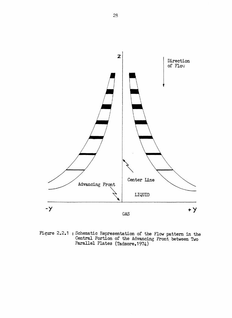
2.2.1 Schematic Representation of the Flow Pattern in the Central Portion of the Advancing Front between two Parallel Plates (Tadmore, 1974) ........................... 28
2.2.2 Flow Pattern in the Advancing Front between Two Parallel Plates (Tadmore, 1974) .............. 29
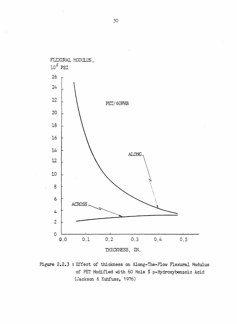
2.2.3 Effect of Thickness on Along-The-Flow Flexural Modulus of PET Modified with 60 Mole % p-Hydroxy-benzoic Acid (Jackson and Kuhfuss, 1976) ......... 30
2.2.4 Schematic Diagram of the Velosity Profile of The Flow behind the Front and its Corresponding Shear Rate ....................................... 31
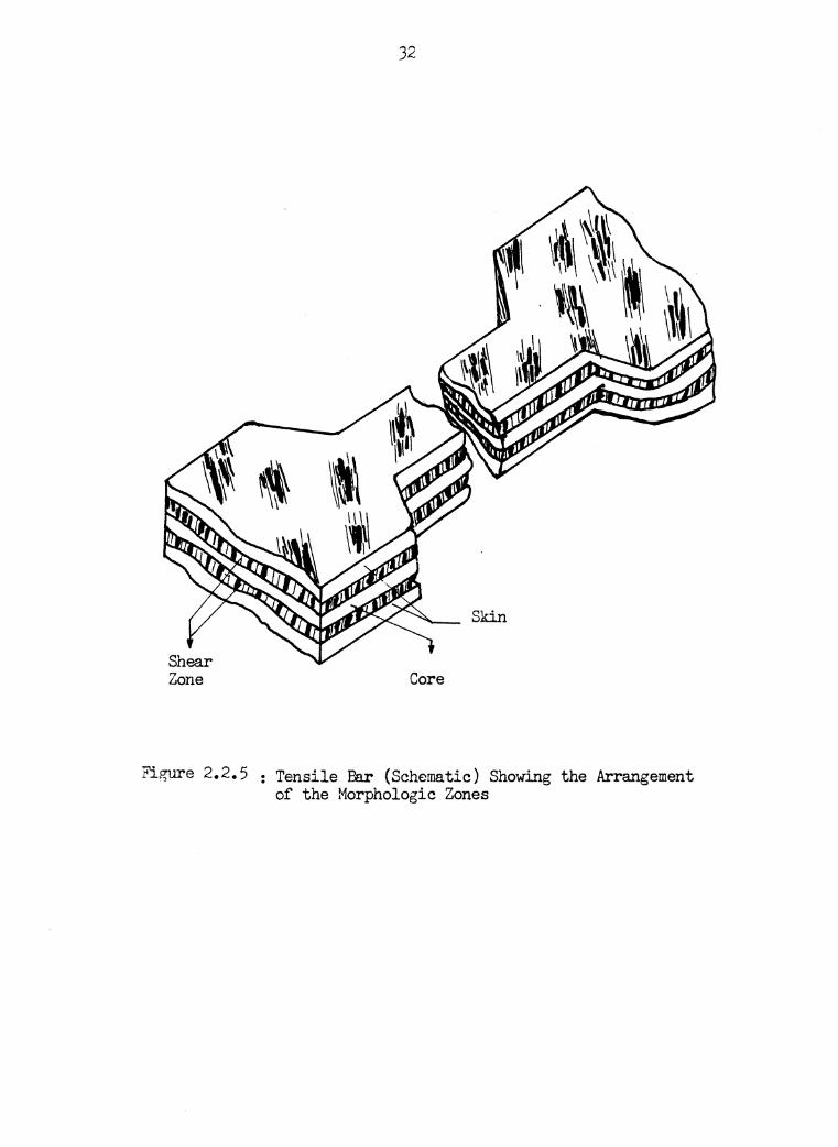
2.2.5 Tensile Bar (Schematic) Showing the Arrangement of the Morphologic Zones (Kantz et al., 1972) .... 32
2.3.1 Mold Filling Patterns in Different Geometry ...... 40
2.3.2 Mold Filling Characteristics in Rectangular Cavity ........................................... 41
3.2.1 Schematic Diagram of Instron Capillary Rheometer (Jerman, 1980) ................................... 49
3.3.1 Injection Molding Apparatus ...................... 53
3.3.2 Runner ........................................... 54
3.3.3 Photograph of Rectangular Mold .................... 55
v
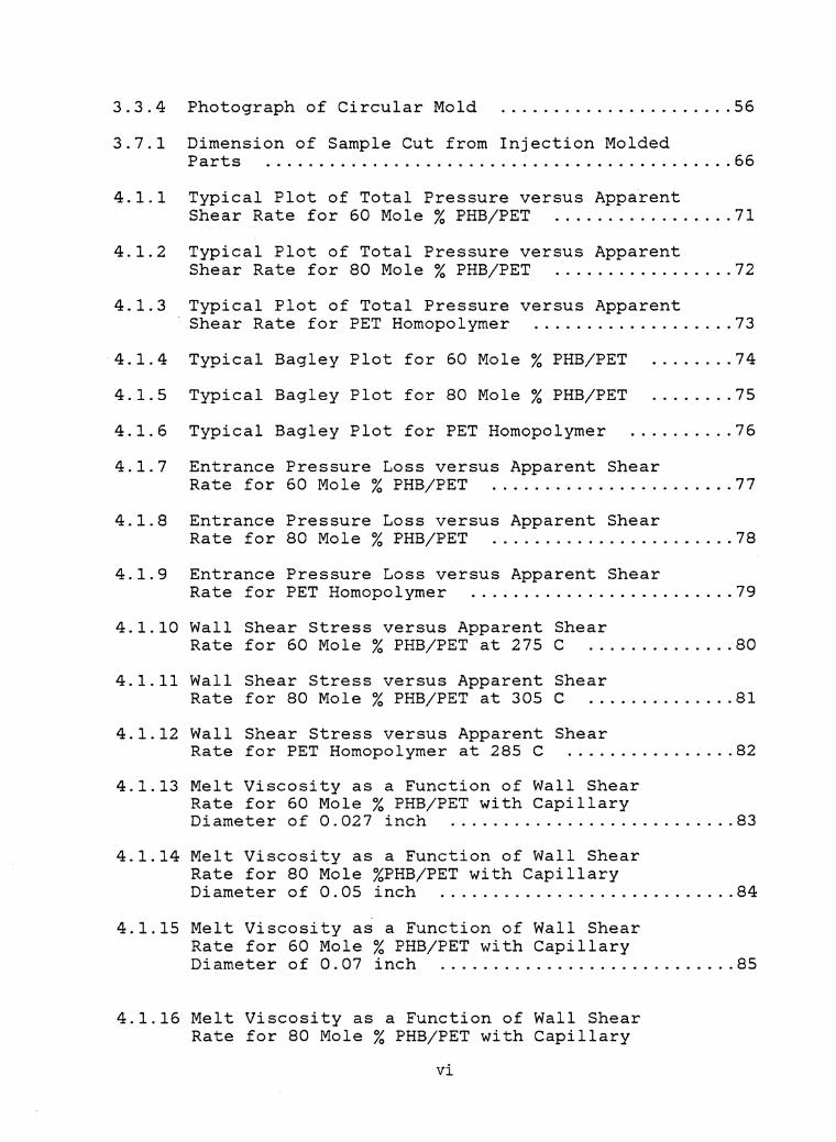
3.3.4 Photograph of Circular Mold ...................... 56
3.7.1 Dimension of Sample Cut from Injection Molded Parts ............................................ 66
4.1.1 Typical Plot of Total Pressure versus Apparent Shear Rate for 60 Mole% PHB/PET ................. 71
4.1.2 Typical Plot of Total Pressure versus Apparent Shear Rate for 80 Mole% PHB/PET ................. 72
4.1. 3 Typical Plot of Total Pressure versus Apparent Shear Rate for PET Homopolymer ................... 7 3
4.1. 4 Typical Bagley Plot for 60 Mole % PHB/PET ........ 7 4
4.1. 5 Typical Bagley Plot for 80 Mole % PHB/PET ........ 7 5
4.1. 6 Typical Bagley Plot for PET Homopolymer .......... 7 6
4.1.7 Entrance Pressure Loss versus Apparent Shear Rate for 60 Mole% PHB/PET ....................... 77
4.1.8 Entrance Pressure Loss versus Apparent Shear Rate for 80 Mole% PHB/PET ....................... 78
4.1.9 Entrance Pressure Loss versus Apparent Shear Rate for PET Homopolymer ......................... 79
4. 1. 10 Wall Shear Stress versus Apparent Shear Rate for 60 Mole % PHB/PET at 275 c .............. 80
4.1.11 Wall Shear Stress versus Apparent Shear Rate for 80 Mole % PHB/PET at 305 c .............. 81
4 .1.12 Wall Shear Stress versus Apparent Shear Rate for PET Homopolymer at 285 c ................ 82
4.1.13 Melt Viscosity as a Function of Wall Shear Rate for 60 Mole % PHB/PET with Capillary Diameter of 0.027 inch ........................... 83
4.1.14 Melt Viscosity as a Function of Wall Shear Rate for 80 Mole %PHB/PET with Capillary Diameter of 0.05 inch ............................ 84
4.1.15 Melt Viscosity as a Function of Wall Shear Rate for 60 Mole % PHB/PET with Capillary Diameter of 0.07 inch ............................ 85
4.1.16 Melt Viscosity as a Function of Wall Shear Rate for 80 Mole % PHB/PET with Capillary
vi
Diameter of 0.027 inch ........................... 86
4.1.17 Melt Viscosity as a Function of Wall Shear Rate for 80 Mole % PHB/PET with Capillary Diameter of 0.05 inch ............................ 87
4.1.18 Melt Viscosity as a Function of Wall Shear Rate for 80 Mole % PHB/PET with Capillary Diameter of 0. 07 inch ............................ 88
4.1.19 Melt Viscosity as a Function of Wall Shear Rate for PET Homopolymer with Capillary Diameter of 0.027 inch ........................... 89
4. 2. 1 Di stance from Ga.te versus Time for Various Fluid Pigments in a Cold Mold (Mold Temp.= 100 C, Cavity thickness= 0.125 inch, Injection Speed = 40 cm/min) ..................................... 92
4.2.2 Distance from Gate versus Time for Various Fluid pigments in a Hot Mold (Mold Temp.= 200 C, Cavity thickness= 0.125 inch, Injection Speed = 40 cm/min) ..................................... 93
4.2.3 Velocity of Various Fluid Pigments versus Distance from Gate in a Cold Mold (Mold Temp.= 100 C, Cavity thickness= 0.125 inch, Injection Speed = 40 cm/min) ............................... 94
4.2.4 Velocity of Various Fluid Pigments versus Distance from Gate in a Hot Mold (Mold Temp.= 200 C, Cavity Thickness= 0.125 inch, Injection Speed = 40 cm/min) ............................... 95
4.2.5 Longitudinal Section of Short-Shot Type of Injection for 60 Mole% PHB/PET .................. 96
4.2.6 Longitudinal Section of Short-Shot Type of Injection for 80 Mole% PHB/PET .................. 97
4.2.7 Longitudinal Section of Short-Shot Type of Injection for PET Homopolymer .................... 98
4.2.8 Photograph of Section Cut Transverse to the Flow Direction ........................................ 99
4.3.1 Shrinkage of the Microtomed Samples of 60 Mole % PHB/PET (Mold Temp. = 100 C, Melt Temp.= 275 C, Injection Speed= 20 cm/min., Cavity thickness= 0.1250 inch) ................... 102
4.3.2 Shrinkage of the Microtomed Samples of 60 Mole % PHB/PET (Mold Temp.= 100 C, Melt Temp. = 285 C, Injection Speed= 20 cm/min.,
vii

Cavity Thickness= 0.125 inch) .................. 103
4.3.3 Shrinkage of the Microtomed Samples of 80 Mole % PHB/PET (Mold Temp.= 100 C, Melt Temp. = 305 c, Injection Speed= 20 cm/min., Cavity Thickness= 0.1250 inch) ................. 104
4.3.4 Shrinkage of the Microtomed Samples of 60 Mole % PHB/PET (Mold Temp.= 100 C, Melt Temp. = 275 C, Injection Speed= 40 cm/min., Cavity Thickness= 0.1250 inch) ................. 105
4.3.5 Shrinkage of the Microtomed Samples of 60 Mole % PHB/PET (Mold Temp.= 100 C, Melt Temp. = 285 C, Injection Speed= 40 cm/min., Cavity Thickness= 0.1250 inch) ................. 106
4.3.6 Shrinkage of the Microtomed Samples of 80 Mole % PHB/PET (Mold Temp.= 100 C, Melt Temp. = 305 C, Injection Speed= 40 cm/min., Cavity Thickness= 0.1250 inch) ................. 107
4.3.7 Shrinkage of the Microtomed Samples of 60 Mole % PHB/PET (Mold Temp.= 100 C, Melt Temp. = 275 C, Injection Speed= 20 cm/min., Cavity Thickness= 0.0625 inch) ................. 108
4.3.8 Shrinkage of the Microtomed Samples of 60 Mole % PHB/PET (Mold Temp.= 100 C, Melt Temp. = 285 C, Injection Speed= 20 cm/min., Cavity Thickness= 0.0625 inch) ................. 109
4.3.9 Shrinkage of the Microtomed Samples of 80 Mole % PHB/PET (Mold Temp.= 100 C, Melt Temp. = 305 C, Injection Speed= 20 cm/min., Cavity Thickness= 0.0625 inch) ................. 110
4.3.10 Shrinkage of the Microtomed Samples of 60 Mole % PHB/PET (Mold Temp.= 100 C, Melt Temp. = 275 C, Injection Speed= 40 cm/min., Cavity Thickness= 0.0625 inch) ................. 111
4.3.11 Shrinkage of the Microtomed Samples of 60 Mole % PHB/PET (Mold Temp.= 100 C, Melt Temp. = 285 C, Injection Speed= 40 cm/min., Cavity Thickness= 0.0625 inch) ................. 112
4.3.12 Shrinkage of the Microtomed Samples of 80 Mole % PHB/PET (Mold Temp.= 100 C, Melt Temp. =305 C, Injection Speed= 40 cm/min., Cavity Thickness= 0.0625 inch) ................. 113
4.3.13 Shrinkage of the Microtomed Samples of 60 Mole % PHB/PET (Mold Temp.= 165 C, Melt
viii

Temp. = 275 C, Injection Speed= 20 cm/min., Cavity Thickness= 0.1250 inch) ................. 114
4.3.14 Shrinkage of the Microtomed Samples of 60 Mole % PHB/PET (Mold Temp.= 165 C, Melt Temp. = 285 C, Injection Speed= 20 cm/min., Cavity Thickness= 0.1250 inch) ................. 115
4.3.15 Shrinkage of the Microtomed Samples of 60 Mole % PHB/PET (Mold Temp.= 165 C, Melt Temp. = 275 C, Injection Speed= 40 cm/min., Cavity Thickness= 0.1250 inch) ................. 116
4.3.16 Shrinkage of the Microtomed Samples of 60 Mole % PHB/PET (Mold Temp.= 165 C, Melt Temp. = 285 C, Injection Speed= 40 cm/min., Cavity Thickness= 0.1250 inch) ................. 117
4.3.17 Shrinkage of the Microtomed Samples of 60 Mole % PHB/PET (Mold Temp.= 165 C, Melt Temp. = 275 C, Injection Speed= 20 cm/min., Cavity Thickness= 0.0625 inch) ................. 118
4.3.18 Shrinkage of the Microtomed Samples of 60 Mole % PHB/PET (Mold Temp.= 165 C, Melt Temp. = 285 C, Injection Sp~ed = 20 cm/min., Cavity Thickness= 0.0625 inch) ................. 119
4.3.19 Shrinkage of the Microtomed Samples of 60 Mole % PHB/PET (Mold Temp.= 165 C, Melt Temp. = 275 C, Injection Speed= 40 cm/min., Cavity Thickness= 0.0625 inch) ................. 120
4.3.20 Shrinkage of the Microtomed Samples of 60 Mole % PHB/PET (Mold Temp.= 165 C, Melt = Temp. = 285 C, Injection Speed= 40 cm/min., Cavity Thickness= 0.0625 inch) ................. 121
4.3.21 Comparison of the Across the Flow Shrinkage of The Microtomed Samples of 60 Mole % PHB/PET in two Seperate Runs (Injection Speed = 20 cm/min, Cavity Thickness= 0.125 inch) .................. 122
5.1.1 Viscosity versus Wall Shear Rate for PET/60%PHB at 260 c ........................................ 12 8
5.1.2 Viscosity versus Wall Shear Rate for PET/60%PHB at 275 c ........................................ 12 9
5.1.3 Viscosity versus Wall Shear Rate for PET/60%PHB at 285 c ........................................ 13 0
5.1.4 Viscosity versus Wall Shear Rate for PET/80%PHB at 305 c ........................................ 131
ix

5.1.5 Viscosity versus Wall Shear Rate for PET/80%PHB at 315 C ........................................ 132
5.1.6 Viscosity versus Wall Shear Rate for PET Homopolymer at 275 C ....... ~· ................... 133
5.1.7 Viscosity versus Wall Shear Rate for PET Homopolymer at 285 C ............................ 134
5.1.8 Schematic Diagram of Capillary Used in This Work (A) and That Used by Jerman (B), (Jerman, 1980) .................................. 135
5.2.1 Comparison of Viscosity for PET/60%PHB Measured at 260 C Using Capillaries with Different Diameters ........................ 141
5.2.2 Comparison of Viscosity for PET/60%PHB Measured at 275 C Using Capillaries with Different Diameters ........................ 142
5.2.3 Comparison of Viscosity for PET/60%PHB Measured at 285 C Using Capillaries with Different Diameters ........................ 143
5.2.4 Comparison of Viscosity for PET/80%PHB Measured at 305 C Using Capillaries with Different Diameters ........................ 144
5.2.5 Comparison of Viscosity for PET/60%PHB Measured at 315 C Using Capillaries with Different Diameters ........................ 145
5.2.6 Entrance Pressure Loss as Function of Apparent Shear Rate for 60 Mole % PHB/PET Measured at 260 C Using Capillary with Different Diameters .. 146
5.2.7 Entrance Pressure Loss as Function of Apparent Shear Rate for 60 Mole % PHB/PET Measured at 275 C Using Capillary with Different Diameters .. 147
5.2.8 Entrance Pressure Loss as Function of Apparent Shear Rate for 60 Mole % PHB/PET Measured at 285 C Using Capillary with Different Diameters .. 148
5.2.9 Entrance Pressure Loss as Function of Apparent Shear Rate for 80 Mole % PHB/PET Measured at 305 C Using Capillary with Different Diameters .. 149
5.2.10 Entrance Pressure Loss as Function of Apparent Shear Rate for 80 Mole % PHB/PET Measured at 315 C Using Capillary with Different Diameters .. 150
x
5.2.11 Viscosity versus Wall Shear Rate for 60 Mole% PHB/PET at 275 C (without Correcting for Pressure Entrance Loss) .................................. 151
5.3.1 Distribution of Colors in a Molded Plaque of PET Homopolymer (Mold Temp.= 100 C, Melt Temp.= 285 C, Injection Speed= 40 cm/min) .................... 156
5.3.2 Velocity of Various Fluid Pigments versus Time for PET Homopolymer (Mold Temp.= 285 C, Injection Speed = 40 cm/min, Cavity Thickness= 0.1250 inch) ................. 157
5.3.3 Longitudinal Section of Short-Shot type of Injection for 60 Mole% PHB/PET ................. 158
5.3.4 Longitudinal Section of Short-Shot type of Injection for 80 Mole% PHB/PET ................. 159
5.3.5 Proposed Mold Filling Mechanism for PET/PHB Copolymer Systems ............................... 160
5.4.1 Schematic Representation of the Bulk Structure of Liquid Crystalline Copolymers of PET modified with 60 and 80 Mole% PHB ....................... 168
5.4.2 Effect of Injection Speed on Shrinkage of Microtomed Samples Transverse to the Flow Direction for 60 Mole % PHB/PET (Mold Temp. = 100 C, Melt Temp. = 275 C Cavity Thickness= 0.125 inch) .................. 169
5.4.3 Effect of Injection Speed on Shrinkage of Microtomed samples Transverse to the Flow Direction for 60 MOle % PHB/PET (Mold Temp.= 100 C, Melt Temp.= 285 C, Cavity Thickness= 0.125 inch) .................. 170
5.4.4 Effect of Injection Speed on Shrinkage of Microtomed Samples Transverse to the Flow Direction for 80 Mole % PHB/PET (Mold Temp.= 100 C, Melt Temp.= 305 C, Cavity Thickness= 0.125 inch) .................. 171
5.4.5 Effect of Injection Speed on Shrinkage of Microtomed Samples Transverse to the Flow Direction for 60 Mole % PHB/PET (Mold Temp.= 100 C, Melt Temp.= 275 C, Cavity Thickness= 0.0625 inch) ................. 172
5.4.6 Effect of Injection Speed on Shrinkage of Microtomed Samples Transverse to the Flow Direction for 60 Mole % PHB/PET (Mold Temp.= 100 C, Melt Temp. = 285 C,
xi

Cavity Thickness= 0.0625 inch) ................. 173
5.4.7 Effect of Injection Speed on Shrinkage of Microtomed Samples Transverse to the Flow Direction for 80 Mole % PHB/PET (Mold Temp.= 100 C, Melt Temp.= 305 C, Cavity Thickness= 0.0625 inch) ................. 174
5.4.8 Effect of Cavity Thickness on Shrinkage Transverse to the Flow Direction for 60 Mole % PHB/PET (Mold Temp. = 100 C, Melt Temp.= 275 C, Injection Speed= 20 cm/min) ................... 175
5.4.9 Effect of Cavity Thickness on Shrinkage Transverse to the Flow Direction for 60 Mole % PHB/PET (Mold Temp. = 100 C, Melt Temp.= 285 C, Injection Speed= 20 cm/min) .................... 176
5.4.10 Effect of Cavity Thickness on Shrinkage Transverse to the Flow Direction for 80 Mole % PHB/PET (Mold Temp. = 100 C, Melt Temp.= 305 C, Injection Speed= 20 cm/min) .................... 177
5.4.11 Effect of Cavity Thickness on Shrinkage Transverse to the Flow Direction for 60 Mole % PHB/PET (Mold Temp. = 100 C, Melt Temp.= 275 C, Injection Speed= 40 cm/min) .................... 178
5.4.12 Effect of Cavity Thickness on Shrinkage Transverse to the Flow Direction for 60 Mole % PHB/PET (Mold Temp. = 100 C, Melt Temp.= 285 C, Injection Speed= 40 cm/min) .................... 179
5.4.13 Effect of Cavity Thickness on Shrinkage Transverse to the Flow Direction for 80 Mole % PHB/PET (Mold Temp. = 100 C, Melt Temp.= 305 C, Injection Speed= 40 cm/min) .................... 180
5.4.14 Effect of Injection Speed on Shrinkage of Microtomed Samples for 60 Mole % PHB/PET (Mold Temp. = 165 C, Melt Temp.= 275 C, Cavity Thickness= 0.125 inch) .................. 181
5.4.15 Effect of Injection Speed on Shrinkage of Microtomed Samples for 60 Mole % PHB/PET (Mold Temp. = 165 C, Melt Temp.= 285 C, Cavity Thickness= 0.125 inch) .................. 182
5.4.16 Effect of Injection Speed on Shrinkage of Microtomed Samples for 60 Mole % PHB/PET (Mold Temp. = 165 C, Melt Temp.= 275 C, Cavity Thickness= 0.0625 inch) ................. 183
5.4.17 Effect of Injection Speed on Shrinkage of
xii
Microtomed Samples for 60 Mole % PHB/PET (Mold Temp. = 165 C, Melt Temp.= 285 C, Cavity Thickness= 0.0625 inch) ................. 184
5.4.18 Effect of Cavity Thickness on Shrinkage of Microtomed Samples for 60 Mole % PHB/PET (Mold Temp. = 165 C, Melt Temp.= 275 C, Injection Speed= 20 cm/min) .................... 185
5.4.19 Effect of Cavity Thickness on Shrinkage of Microtomed Samples for 60 Mole % PHB/PET (Mold Temp. = 165 C, Melt Temp.= 285 C, Injection Speed= 20 cm/min) .................... 186
5.4.20 Effect of Cavity Thickness on Shrinkage of Microtomed Samples for 60 Mole % PHB/PET (Mold Temp. = 165 C, Melt Temp.= 275 C, Injection Speed= 40 cm/min) .................... 187
5.4.21 Effect of Cavity Thickness on Shrinkage of Microtomed Samples for 60 Mole % PHB/PET (Mold Temp. = 165 C, Melt Temp.= 285 C, Injection Speed= 40 cm/min) .................... 188
xiii

LIST OF TABLES
3.1.1 Temperature for Viscosity Measurement of Poly (Ethylene Terephthalate) and its Copolymer of PET & p-hydroxybenzoic Acid ...................... 46
3.2.1 Gear Ratio and Speeds for Instron Model 3211 Capillary Rheometer .............................. 50
3.5.1 Compression Molding Temperature for PET and its Copolymer with PHB ............................... 61
3.6.1 Injection Molding Conditions ..................... 64
3.7.1 Annealing Time and Temperature for Shrinkage Measurement ...................................... 67
xiv
Chapter I
INTRODUCTION
Liquid crystalline polymers are materials which possess
fluid-like mechanical properties but also are capable of
transmitting polarized light under static conditions, and in
some cases, they exhibit Bragg diffraction of X-rays (Wen-
droff, 1978). These optical properties are the result of a
high degree of molecular order in the fluid state of the po-
lymer. Thermodynamically, the liquid crystalline state is a
stable state existing between the solid and fluid phases and
is, therefore, referred to as a mesophase or ~ mesomorphic
state (Wendroff, 1978). For polymer to possess this meso-
morphic state, the structure of the molecule is invariably
highly ~anisotropic in shape, usually rod-like or lath-like
and composed of a rigid central section with some flexible
end group (Wissbrun, 1981).
Liquid crystalline polymeric systems have received con-
siderable interest in recent years for several reasons.
First, a study of liquid crystalline polymer literature re-
veals that liquid crystalline polymers in the solid state
possess exceptional physical and mechanical properties which
arise as a result of molecular structure and orientation
generated in the fluid state. Secondly, processing of these
1

2
materials can be carried out more rapidly with less expendi-
ture of energy due to lower viscosity than that of polymers
with the same molecular weight in the isotropic state.
Furthermore, liquid crystalline polymers may be spun to pro-
duce ultra-high strength fibers (Morgan, 1976).
Recent studies focussing on synthesis and rheology of
thermotropic liquid crystalline copolymers of polyethylene
terephthalate (PET) modified with p-hydroxybenzoic acid
(PHB) have appeared in the literature (Jackson &: Kuhfuss,
1976; Wissbrun, 1980; Jerman&: Baird, 1981). By increasing
the mole percent of PHB in the chain, the chain stiffness is
increased to the point that is sufficient to yield a polymer
system which exhibits liquid crystalline behavior (McFarlane
et al., 1977). The physical properties of injection molded
specimens of these materials were reported to be highly ani-
sotropic. Physical properties measured al·ong the flow direc-
tion were exceptionally higher than those measured across to
the flow direction. Furthermore, these properties were de-
pendent on melt temperature and the dimension of the mold.
In particular, they found that the physical properties were
highly dependent on the thickness of the mold and increasing
with decreasing mold thickness. According to these authors,
this is probably due to an increa·se in orientation as the
result of high shear rates and the increased cooling rate
3
which resulted in preserving more of the orientation pro-
duced during flow.
In general,the final properties of the injection molded
parts are directly related to its molecular orientation in
the melt state and its processed condition. This molecular
orientation may be influenced by a layer of molecules at the
boundary with different molecular orientation than those in
the core fluid. Fisher and Fredrickson (1969) have reported
this influence on viscosity of low molecular weight liquid
crystalline polymer. Leslie and Ericksen have developed
constitutive theories f0r nematic liquid crystalline fluids
which lead to the prediction that the viscosity depends on
some characteristic width, i.e. radius of the capillary, as
well as on shear rate. Because of this influence of the
boundary, the r,heological properties of liquid crystalline
polymer may change with the size of the flow channel, i.e.
radius of the capillary. In turn, the mechanical and physi-
cal properties of the molded parts may also be changed. It
is the purpose of this study to investigate this boundary
layer effect on the rheological property of the thermotropic
liquid crystalline polymer of PET modified with 60 and 80
mole % PHB. In particular, viscosities 9f these polymers
will be measured using different capillary diameters to det-
ermine whether viscosity depends on capillary diameter as
4
predicted from the liquid crystalline continuum theory de-
veloped by Ericksen (1969) and Leslie (1969).
The final physical properties of any injection molded
specimen depend on the molecular orientation generated in
the filling stage of injection molding. In this study, the
mold filling characteristics of PET/PHB copolymer in both
unidirectional flow and radial flow will be investigated by
means of a tracer technique. Pigmented fluid elements will
be used as tracers to illustrate flow patterns.
The fact that physical properties of injection molded
specimens of PET/60PHB are highest at 275°C as stated in the
publication of Jackson & Kuhfuss (1976) will be further stu-
died by injection molding this polymer at different melt
temperatures in an Instron rheometer. By microtoming the
injection molded parts, shrinkage measurement will be per-
formed to qualitatively determine the molecular orientation
of the molded test specimens. This, in turn, may help to
explain the dependence of the mechanical properties of these
materials on melt temperature and mold thickness.
Injection molding of these copolyesters in end-gate cavi-
ties leads to plaques which have anisotropic properties.
Studies will also be carried out using a center-gate disc
cavity in order to investigate the' possibility for obtaining
biaxial orientation.

Chapter II
LITERATURE REVIEW
The final mechanical properties of injection molded spe-
cimens of poly (ethylene terephthalate) modified with p-hy-
droxybenzoic acid are excellent and highly anisotropic. To
understand the reasons for these unusually high mechanical
properties, one must know its liquid crystalline behavior.
Therefore, the first section in this chapter will review the
nature of liquid crystalline polymers in general and specif-
ically the poly (ethylene terephthalate) modified with p-hy-
droxybenzoic acid. Since the mechanical properties are re-
lated with the skin-core formation generated during mold
filling process, the next section in this chapter will re-
view the mold filling mechanism in a rectangular cavity and
the skin-core morphology of the injection molded specimen.
Last, injection molding studies for different shape of molds
are also included in this chapter.
5
6
2.1 LIQUID CRYSTALLINE ORDER
2.1.1 General
A liquid crystalline polymer is one which exhibits physi-
cal and mechanical properties of regular fluids. However, it
also has a high degree of molecular order which is somewhat
characteristic of a crystalline solid. This high degree of
molecular order can be detected by light scattering, X-ray
techniques, or Bragg reflections of X-ray (Wendroff 1978).
This order occurs in many different forms and may exist in
local regions in either the melt state or solution. Because
of this ordering, liquid crystalline polymers have been
classified into thermotropic and lyotropic mesophases. Ther-
motropic liquid crystals are materials that are transformed
into a mesophase simply by heating these materials above
their melting points. Lyotropic liquid crystals mesophases
are formed by increasing the concentration of polymer in so-
lution. Soap and water is a typical example of liquid crys-
tals of this type. The distinction between thermotropic and
lyotropic liquid crystal is not exclusive, however. For lyo-
tropic case, the degree of liquid crystallinity is a func-
tion of both concentration and temperature. Any change in
temperature may affect the critical concentration, the con-
centration at which liquid crystalline domains are formed.
Therefore, for a lyotropic liquid crystal, transitions from
7
thermotropic to isotropic state can occur by changing both
the temperature and concentration of the solution.
Depending on the nature of the ordering, liquid crystal-
line polymers may be classified into three mesophases: ne-
matic, smectic, and cholesteric. The nematic mesophase is
one in which there is no long-range order of the position of
the molecule. In this mesophase, molecules tend to line up
in a preferred direction which is described by a "director".
The distribution of the director among the molecules is
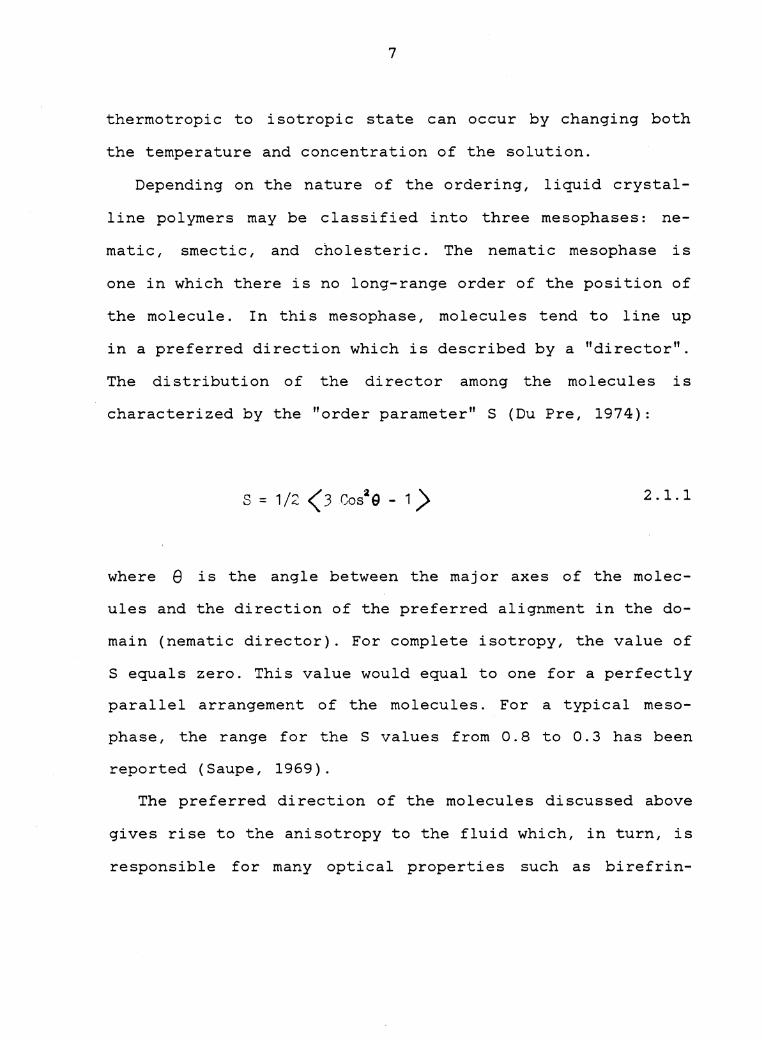
characterized by the "order parameter" S (Du Pre, 1974):
S = 1 /2 < 3 Cos2 6 - 1 ) 2 .1.1
where e is the angle between the major axes of the molec-
ules and the direction of the pref erred alignment in the do-
main (nematic director). For complete isotropy, the value of
S equals zero. This value would equal to one for a perfectly
parallel arrangement of the molecules. For a typical meso-
phase, the range for the S values from 0.8 to 0.3 has been
reported (Saupe, 1969).
The preferred direction of the molecules discussed above
gives rise to the anisotropy to the fluid which, in turn, is
responsible for many optical properties such as birefrin-

8
gence (Tsvetkov et al., 1978), NMR splitting (Mcfarlane et
al., 1977) and light scattering (Wendroff, 1978). For the
systems displaying high strength or high modulus, it is gen-
erally the nematic morphology that is preferrably induced.
Because of the preferred direction of the molecules, the
nematic director can be easily influenced by interacting
with electric and magnetic fields (Filas, 1977) as well as
by shear (Porter and Johnson, 1967). In the proximity of the
surface, the molecules may be oriented at some angle to the
surface, forming a boundary layer of the molecules. This an-
gle is a strong function of the physical and chemical treat-
ment of that surface (Fisher and Fredrickson, 1969).
Similarly to the nematic mesophases,the cholesteric meso-
phases possess a preferred direction and do not exhibit
long-range positional order. However, unlike nematics, the
direction in space of the "director" varies helically along
an axis perpendicular to the plane in which the director
lies as shown schematically in figure 2.1.1 (Wissbrun,
1981). If the pitch of the helical structure is similar to
the wavelength of visible light, a selective reflection of
monochromatic light can be observed. This effect leads to
the irridescent colors often observed in cholesteric meso-
phases (Wendroff, 1978). Due to the lack of the overlap bet-
ween the long axis of the molecules, polymer systems of this

9
type do not possess high strength or high modulus in con-
trast to that of purely nematic mesophase.
Among the three types of ordering, smectic is the most
ordered mesophase. In smectics, the molecules are arranged
in well-defined layers so that they do have a long range po-
si tional order in one dimension which is perpendicular to
the layer plane (Wissbrun, 1981). Since smectic liquid crys-
tals possess a higher degree of order than that seen in the
nematic mesophase, it is natural to assume that the S values
will be higher. This is indeed the case. The S values for
this mesophase have been reported as high as 0. 9 (Du Pre,
1974). Al though possessing the highest degree of ordering,
materials having smectic morphology do not exhibit high
strength or high modulus. This is due to the lack of mole-
cular backbone overlap in the orientation direction.
2 .1.2 The Thermotropic Liquid Crytalline System of Poly (Ethylene Terephthalate) and p-Hydroxybenzoic Acid
Although poly (ethylene terephthalate), (PET), is widely
used in the fiber and film industry, it has only limited ac-
ceptance as a molding plastic. The reason for this is the
need of a hot mold (140-150°C) to allow the polymer to crys-
tallize (Jackson & Kuhfuss, 1976). In an attemp to solve
this problem and also to meet certain specific flammability
standards, the amount of aromatic character of PET was in-
10
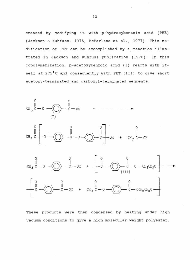
creased by modifying it with p-hydroxybenzoic acid ( PHB)
(Jackson & Kuhfuss, 1976; Mcfarlane et al., 1977). This mo-
dification of PET can be accomplished by a, reaction illus-
trated in Jackson and Kuhfuss publication ( 1976). In this
copolymerization, p-acetoxybenzoic acid (I) reacts with it-
self at 275°C and consequently with PET (III) to give short
acetoxy-terminated and carboxyl-terminated segments.
0 II
C"l c- 0 u3 .I
0
-@-~-OH (I)
II II 11 ot o ot· c o--<Q>--c-o-@-c OH +
0 II
Cu c o·· •l 3 - ti
0 0 11~11
CP. 3 C - 0 --0--- C - OE + r ~ ~ ~-o- cn,cn,of-t (III)
+ g --@--L OII + CE 3 L 0 --@-- ~ - OCH2 CE, 0 ~
These products were then condensed by heating under high
vacuum conditions to give a high molecular weight polyester.
11
II II 11 0 0 0 -t C --@-- C - 0--@-- C - OC.:I 2CH 20 +
0 II
Cµ COTT ... ~ 3 ti
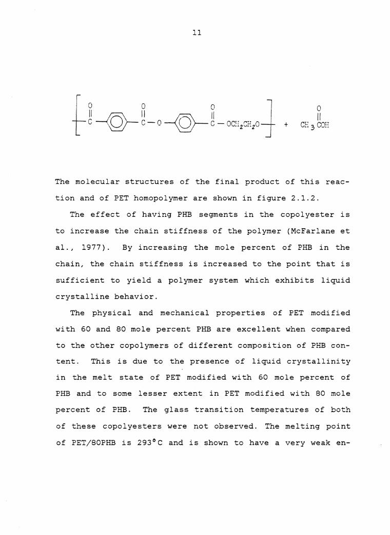
The molecular structures of the final product of this reac-
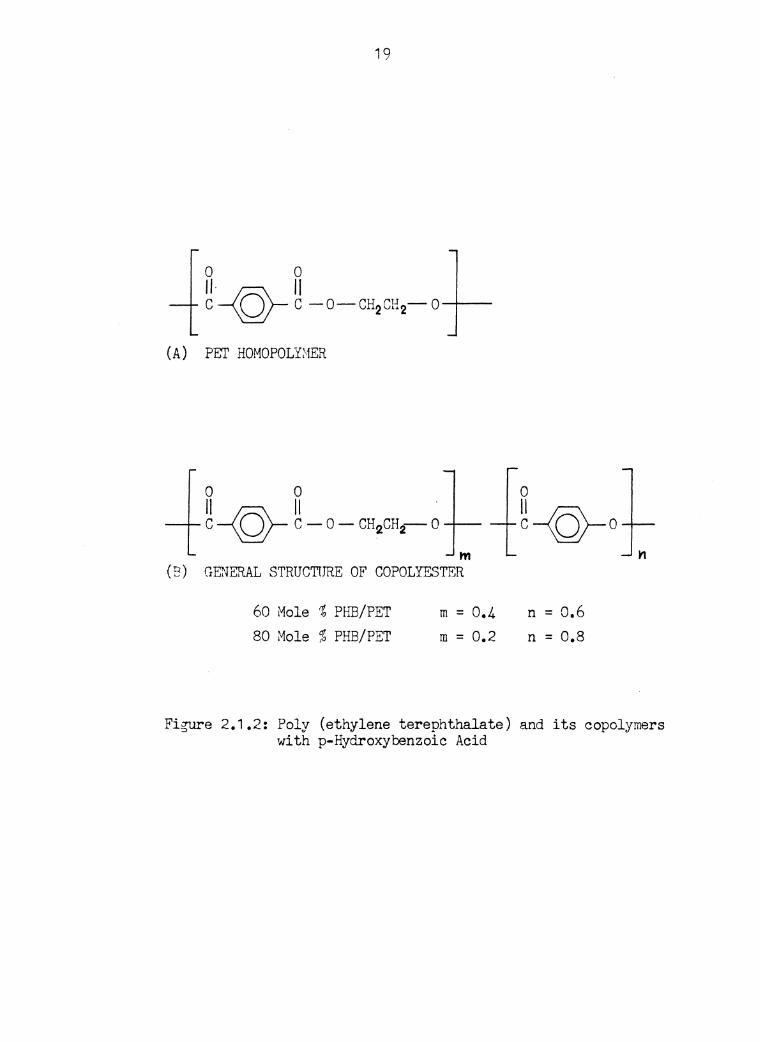
tion and of PET homopolymer are shown in figure 2.1.2.
The effect of having PHB segments in the copolyester is
to increase the chain stiffness of the polymer (McFarlane et
al., 1977). By increasing the mole percent of PHB in the
chain, the chain stiffneas is increased to the point that is
sufficient to yield a polymer system which exhibits liquid
crystalline behavior.
The physical and mechanical properties of PET modified
with 60 and 80 mole percent PHB are excellent when compared
to the other copolymers of different composition of PHB con-
tent. This is due to the presence of liquid crystallinity
in the melt state of PET modified with 60 mole percent of
PHB and to some lesser extent in PET modified with 80 mole
percent of PHB. The glass transition temperatures of both
of these copolyesters were not observed. The melting point
of PET/80PHB is 293°C and is shown to have a very weak en-
12
do therm while the melting point of PET/60PHB has not been
observed. The later phenomena is probably due to the forma-
tion of liquid crystallinity.
Probably, one of the most unusual properties of these co-
polyesters is the melt viscosity. The effect of PHB contents
on melt viscosity at 275°c is shown in figure 2.1.3. It is
noteworthy that the melt viscosities increased as the PHB
content was increased to about 30 mole percent and then de-
creased as the PHB content was increased further to 60 mole
percent. The effect of the shear on melt viscosities of
these copolyesters at 275°C is shown in figure 2.1.4. As the
PHB content increases, the polymer becomes shear-sensitive
at lower shear rates.
The mechanical properties of the injection molded speci-
mens of these copolymers are exceptionally high. When com-
pared to the same copolymers with different PHB content, PET
modified with 60 mole percent PHB is reported to have maxi-
mum flexural modulus, Izod impact strength, and minimum
Rockwell hardness. The absence of mold Shrinkage in composi-
tion containing 40.,-80 mole percent PHB is also reported.
This is probably due to the long relaxation time of these
polymers (Jackson & Kuhfuss, 1976).
The unusual high mechanical properties of liquid crystal-
line polymers probably arose from the orientation generated
13
in the melt state. Especially, in injection molding, the ef-
fect of molecular orientation on the mechanical properties
is more pronounced. For 60 mole percent PHB, as the tempera-
ture of the melt increases from 210°c to 260°C, the melt
viscosity decreased. If the speed of the polymer melt in-
jected into the mold increased, the orientation of the po-
lymer chains therefore would increase (Jackson &. Kuhfuss,
1976). The melt temperature at which this copolyester is
injection molded affects the orientation of the liquid crys-
tal polymer chains and therefore affects its mechanical
properties. The mechanical properties of PET/60PHB increase
as the melt temperature increases from 210 to 260°C. Above
280°C, the properties seem to decrease. According to Jackson
and Kuhfuss (1976), this decrease is probably due to some
loss of orientation of the polymer chains in the melt before
the solidification of the melt takes place.
The nature of the liquid crystalline polymer melt causes
it to be easily oriented by the shear force and extentional
flow during injection. Since the mechanical properties in-
crease as the degree of orientation of the copolyester in-
creases, it is expected that the properties of the "along
the flow direction" are higher than those of "across the
flow direction". In fact, this is observed in the work of
Jackson and Kuhfuss (1976). For 60 and 80 mole percent PHB,

14
the mechanical properties are reported to be highly aniso-
tropic. It is also reported that the mold shrinkage and
coefficient of linear thermal expansion are zero along the
flow direction but not across the flow direction.
In summary, the mechanical properties of injection molded
specimens of PET/PHB copolymer system are highly anisotrop-
ic. These properties are directly related with the molecu-
lar orientation generated in the melt state. Since the de-
gree of molecular orientation in a molded specimen depends
on the melt temperature, mold temperture, specimen's shape
and thickness etc, the mechanical properties are strongly
dependent of these same variables (McFarlane et al., 1977).
The phenomena of low melt viscosities and anisotropic prop-
erties can be explained on the basis of liquid crystalline
formation.
2 .1. 3 Rheological Properties Of Thermotropic Liquid Crystalline Polymers
In recent years there have been a number of papers con-
cerned with the rheology of lyotropic liquid crystalline po-
lymers and a variety of interesting effects; e.g concentra-
tion dependence of viscosity, long relaxation time, apparent
yield stress, and negative normal stress have been observed
(Baird, 1978). Not many comparable studies has been reported
on thermotropic liquid crystalline polymer besides some mea-
15
surements of viscosity as a function of temperature and of
shear rate for the copolyester of poly (ethylene terephth-
late) and p-hydroxybenzoic acid (Jackson and Kuhfuss, 1976;
Jerman and Baird, 1981). Wissbrun (1980) measured the rheo-
logical properties of PET modified with 60 mole percent PHB
using a Rheometrics Mechanical Spectrometer and a capillary
rheometer. In his work, Wissbrun reported a long relaxation
time for the melt, estimated from shear rate dependence of
viscosity and from melt elasticity. The long relaxation time
is presumably associated with the rotation of whole molec-
ules (or of units composed of many segments}, or perhaps of
the cooperative motion of many such molecules or units.
Wissbrun (1980) also observed many cases of unusual flow
behavior including rheopexy in some compositions, negative
normal stresses, and negligible die swell. The rheopexy phe-
nomena is explained to be due to the presence of "a struc-
ture of some sort in the melt." In systems that have an ap-
parent yield stress, but do not show appreciable thixotropy,
the time required for the formation of the structure res-
ponssible for the yield stress must be small compared to the
time between successive measurements. What that structure
might be is not stated clearly in his publication.
Using an Instron Capillary Rheometer, Jerman and Baird
(1981) measured viscosities and die swell of PET/60PHB and

16
PET/80PHB as well as PET homopolymer. The melt viscosity of
PET/60PHB was reported to be considerably lower than that of
PET homopolyrner. This is probably due to the orientation in-
duced from the shear flow and the present of the liquid
crystalline domain in the melt. During flow, these oriented
domains act as the flow unit rather than the individual mo-
lecules. The molecules slide smoothly over each other. Thus
less energy is dissipated than is the case for the randomly
oriented and/or entangled molecules (Jerman and Baird,
1981).
The viscosity of PET/80PHB is higher than that of
PET/60PHB when compared at the same temperature. As reported
by Jackson & Kuhfuss (1976), the PET/80PHB copolyester exhi-
bits a crystalline melting point at 293 ° C, whereas the
PET/60PHB copolyester exhibits neither a glass transition
temperature nor a melting point. Hence the higher viscosity
of PET/80PHB copolymer may be attributed to solidlike re-
gions. However, as the temperature increases, the viscosity
becomes extremely low.
Values of extrudate swell, Dj /D, were reported to in-
crease with increasing melt temperature for both of these
copolymers. This phenomena is probably due to the yield
stresses and negative normal stresses. According to Jerman
and Baird (1981), the lack of extrudate swell could be at-
17
tributed to the yield stresses which inhibit elastic recov-
ery of the extrudate. Furthermore, the shear field in the
capillary is limited to a narrow region near the wall with
the core of the melt passing through the capillary in plug
flow. Therefore, there exists some region in the melt in
which elastic recovery does not occur. At low temperature,
the formation of the yield stresses probably arose from the
crystalline regions. As the melt temperature increases, the
magnitude of the yield stress decreases, thus allowing some
extrudate swell to· occur.
Another possibility which explains this extrudate swell
phenomena is the presence of the negative primary normal
stress differences (N1 ) (Jerman and Baird, 1981). N1 is ne-
gative or negligible when ~/Dis less than or equal to 1.0.
Probably, as temperature increases, the formation of the
isotropic region increases which inturn leads to the posi-
tive values of N and therefore to the values of Dj/D greater
than 1.0. However, if the isotropic regions form, then the
viscosity of the melt is expected to increase but it does
not. These authors suggested that either one or the combina-
tion of these explanations may be respossible for the ob-
served behavior of extrudate swell.

18
NEMATIC
QQQQeG6QQ QQQGeGBUQ QQQQeGIJUQ QOGGeGGQ~ OOQBe~ooo
CHOLESTERIC
r \ r\J\ r\ 0 r, i\\\ (',I\ 0 nu· \j \J \j ·J\).J \J r. "(\ (\(\ .r·\({\ n ~ (\ UU \JU\J U.J\JUU\J 0000\JQ~OOOQ
SMECTIC A Figure 2.1.1: Schematic representation of Mesophase Types
(Wissbrun, 1981)
19
0 0 11~11 C~- C -0-CH2CH 2-0---4---
(A) PET HOMOPOLD,!ER
0 0 0 II -\Q)--11 . C 0 C-0-CH2CH2-0 ~--(Q}--o
m n (2) GENERAL STRUCTURE OF COPOLYESTER
60 Mole % Ph13/PET m = 0.4 n = o.6 80 Mole % PHB/PET m = 0.2 n = 0.8
Figure 2.1.2: Poly (ethylene terephthalate) and its copolymers with p-Hydroxybenzoic Acid

VISCOSITY (275°C), PJISE 105
10 0 20
20
40 60 p-HYDROXYBENZOIC ACID, M)LE %
•
80
SHE..\R RA.TE ,
• 15 0 100 ... 1600 0 54000
100
Figure 2.1.3 : Effect of p-Hydroxybenzoic Acid Content on Melt Viscosity at 275°C (Jackson and Kuhfuss, 1976)
S'""'cC-1

MELT VISCOSITY (275°C), POISE
104
10 1
• PET .A PET/20PHB 6 PET/40PHB 0 PET/SOPHB • PET/60PHB
10
• •
Figure 2.1.4 : Effect of Shear on Melt Visc©sity of PET Modified with p-Hydrox:ybenzoic Acid (Jackson and Kuhfuss, 1976)
22
2.2 THE MECHANISM OF SKIN-CORE FORMATION IN INJECTION MOLDING
The final properties of any injection molded article will
depend on the molecular orientation generated in the melt
state. These properties are also a result of the skin-core
formation in an injection molded article. However, the me-
chanism in which the melt fills in the mold would explain
the skin-core formation and the molecular orientation. It is
obvious, then, that the final properties of an injection
molded article would depend on the mold filling characteris-
tics and the skin-core morphology resulting from this flow.
In this section, the flow of polymer melt in injection mold-
ing is reviewed first. The skin-core morphology generated
from this flow is then discussed.
2.2.1 The Flow Of Polymer Melts In Injection Molding
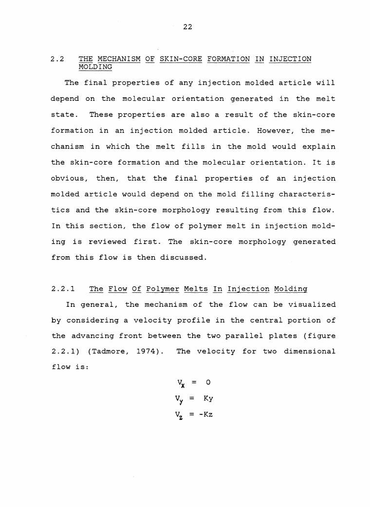
In general, the mechanism of the flow can be visualized
by considering a velocity profile in the central portion of
the advancing front between the two parallel plates (figure
2 . 2 . 1 ) ( Tadmo re, 19 7 4) .
flow is:
The velocity for two dimensional
VX 0
V"t = Ky
Vz = -Kz
23
where K is the rate of elongation. These equations imply
that a rectangular fluid element while moving toward the
front will decelerate in the axial direction, will acceler-
ate in the perpendicular direction, and during this process
will be stretched in the y direction at a constant rate.
In such a steady elongational flow, macromolecules are
stretched and oriented in the y direction. The degree of or-
ientation of these molecules is then dependent on the rate
of elongation. Tadmore (1974) assumed for an order of mag-
nitude calculation that at a distance of 2B upstream of the
front, a fully developed shear flow exists. Therefore, the
rate of elongation is given by the following expression:
- K = Vmax - <v)
2B (2.2.1)
where:
flow
= maximum velocity of the fully developed
<V> = the mean velocity If the power law fluid
model is used in this flow:
2n + 1 n + 1 <v)
Equation (2.2.1) and (2.2.2) can be combined to give:
(2.2.2)
24
- K = n <v) 2(n + 1 )B
(2.2.3)
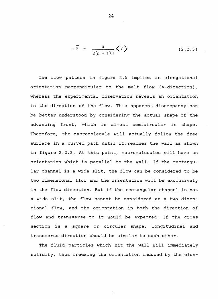
The flow pattern in figure 2. 5 implies an elongational
orientation perpendicular to the melt flow ( y-direction),
whereas the experimental observation reveals an orientation
in the direction of the flow. This apparent discrepancy can
be better understood by considering the actual shape of the
advancing front, which is almost semicircular in shape.
Therefore, the macromolecule will actually follow the free
surface in a curved path until it.reaches the wall as shown
in figure 2.2.2. At this point, macromolecules will have an
orientation which is parallel to the wall. If the rectangu-
lar channel is a wide slit, the flow can be considered to be
two dimensional flow and the orientation will be exclusively
in the flow direction. But if the rectangular channel is not
a wide slit, the flow cannot be considered as a two dimen-
sional flow, and the orientation in both the direction of
flow and transverse to it would be expected. If the cross
section is a square or circular shape, longitudinal and
transverse direction should be similar to each other.
The fluid particles which hit the wall will immediately
solidify, thus freezing the orientation induced by the elon-

25
gational flow. The amount of orientation will depend on the
rate of elongation. Equation (2.2.3) shows that an increase
in injection speed and a decrease in cavity thickness will
result in an increase in orientation. For liquid crystalline
polymers, the latter effect has been observed in the work of
Jackson and Kuhfuss ( 1976). The mechanical properties of
these polymers when measured along the flow are reported to
be higher for the thin cavity than that for the thick cavity
(figure 2.2.3). This measurement indicates that decreasing
cavity thickness will result in an increase in molecular or-
ientation (along the flow only).
The foregoing discussion only addresses the flow mechan-
ism at the flow front. Behind this flow front, an entire
different flow mechanism (shear flow) exists as discussed by
Menges and Wubken (1973). From the section along the flow
direction ( figu.re 2. 2. 4), there exist frozen surface layers
with no motion. The highest velocity gradients, greatest
shear rate, are below the frozen surface layers. Here, the
melt is intensively sheared. This gives rise to a relative
maximum molecular orientation below the frozen surface lay-
ers. Behind the front, as shown in figure 2.2.5, the veloc-
ity vectors of the flow are parallel to the x-axis (flow di-
rection). The average velocity of the melt in this section
is much greater than the velocity of the flow front. There-
26
fore, the melt particles behind the front would rapidly
catch up with it and flow transversally to the front as dis-
cussed earlier in this section.
2.2.2 The Skin-Core Morphology Of Injection Molded Objects
It is generally recognized that the final properties of
injection molded parts are strongly dependent on morphology,
orientation and stress applied during processing (Baer,
1964; Bayer, 1960; Maxwell, 1965; Stein, 1964). Many studies
of various polymers have shown that injection molded objects
have a skin made up of molecules that are highly oriented in
the flow direction and an essentially unoriented central
bulk region which is called a core region. This morphology
has been observed in both glassy and semicrystalline polym-
ers and has been reported throughout the literature (Jackson
and Ballman, 1960; Kantz et al., 1972; Wales, 1972; Ballman
and Toor, 1960). The high degree of molecular orientation in
the skin has been observed in certain instances to cause
warpage, shrinkage and premature fracture during impact and
flexural testing (Keskkula et al., 1965; Morris, 1968).
Optical microscopy shows that the injection molded parts
under any processing condition displayed the skin-core mor-
phology as previously discussed. Kantz et al. (1972) studied
the skin-core formation of a polypropylene tensile bar. They

27
observed that there exist intermediate layers parallel to
the flow direction and between the skin and core. This in-
termediate layer, the shear zone, is spheruli tic and its
morphology differs from that in the core region. The spheru-
li tes are randomly nucleated in the core region while those
in the shear zone are row nucleated. The latter indicates a
higher degree of molecular orientation than that in the core
region. In figure 2. 2. 5, the morphological structure of a
typical tensile bar is shown. This bar is made up of a core,
two layers of shear zones on either side of the core and two
skin zones on each of the two large surfaces.
28
2
Advancing Fr~
-y
Center Ll.ne
LIQUID
GAS
Direction of Flow
+Y
Fi~e 2.2.1 : Schematic Representation of the Flow pattern in the Central Portion of the Advancing Front between Two Parallel Plates (Tadmore,1974)

Advancing Front
29
Cold Wall ---B-----
Figure 2.2.2 Flow Pattern in The Advancing Front Between Two Parallel Plate (Tadmore, 1974)
FLEXURAL MODULUS, 105 PSI
26
24
22
20
18
16
14
12
10
8
6
30
PEI'/60PHB
~\ ~ \
I
\
4
2
ACROSS~
-0
0.0 0.1 0.2 0.3 0.4
TIUCKNESS, IN.
0.5
Figure 2.2.3 : Effect of thickness on Along-The-Flow Flexural Modulus of PET Modified with 60 Mole % p-Hydroxybenzoic Acid (Jackson & Kuhfuss, 1976)

Velocity Profile
,,.--- Solidifying Layer
Shear Rate
Flow Direction
Figure 2.2.4: Schematic Diagram of the Velocity Profile of the Flow Behind the Front and its Correspondin~ Shear Rate
32
Fi~ure 2.2.5 : Tensile Par (Schematic) Showing the Arrangement of the Morphologic Zones
33
2.3 INJECTION MOLDING STUDIES
Injection molding flows are highly complex as a result of
the unsteady and non-isothermal conditions. This process in-
volves the injection of molten plastics into cold, complex
cavities in which they solidify to form fabricated parts.
The mechanical properties of a molded part are strongly de-
pendent on the molding morphological features which in turn
are related to cavity flow as well as packing pressure and
cooling rate (Schmidt, 1977). One qualitative method for in-
vestigating the kinematics of melt flow is to observe flow
patterns in different channels. The first scientific study
of the injection molding process was carried out by Spencer
and Gilmore (1950,1951). In their.publications, the authors
studied the orientation, residual stresses,_ pressure losses
and the fluid mechanics of mold filling. Using a glass win-
dow, these authors observed that polymer melt flows only in
a central region of the mold and there exist stationary lay-
ers next to the mold walls. They proposed that when polymer
melt reaches the advancing front (polymer-air interface), it
contacts the mold wall, cools and stops flowing.
To investigate the flow front as polymer fills up the
mold, many reseachers adapted the flow visualization techni-
que used by Spencer and Gilmore to study mold filling in
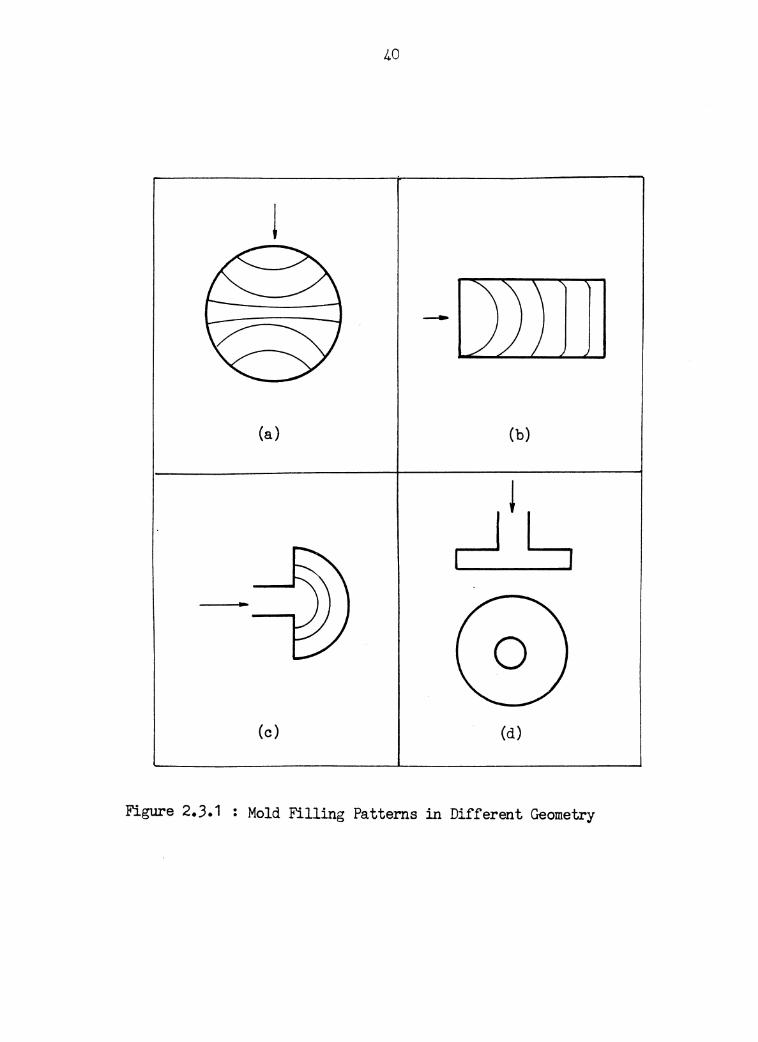
many different complicated geometries. The flow patterns of

34
polystyrene in a disc-shaped cavity were photographed by
Beyer and Spencer (1960). They observed a circular spread-
ing front as shown in figure 2.3.1.a.
More recently, mold filling in a rectangular channel was
investigated visually (figure 2.3.1.b) (White et al., 1974;
Schmidt, 1977). White and Dee (1974) studied mold filling
characteristics of polymer melts in a rectangular mold as
shown in figure 2. 3. 1. b for isothermal and non-isothermal
flows. The apparatus used in their work was a modified In-
stron Rheometer where in stead of a capillary die, a com-
bined nozzle and mold assembly were attatched to the lower
end of the barrel. The mold is primary designed for flow vi-
sualization and the outer clamping blocks are fitted with
Pyrex plate glass windows. For isothermal flow, they ob-
served that there are two basic flow regimes,mold filling
and jetting phenomena, depending upon the injection rate of
the molten polymer into the mold. Figure 2. 3. 2 shows the
slow isothermal flow of polymer melts into a rectangular
mold. The mold filling may be divided into three stages.
First, on passage from the narrow constriction at the gate
into the mold, the melt spreads in an approximately radial
manner. Secondly, after the corner are filled, there is a
transition region in which the front changes from a circular
shape to an almost flat profile. Finally, the nearly flat

35
front continues to move forward un:til the mold is filled.
The front shape seems flat except for some convex curvature
near the mold wall. In this final region, the velocity of
the center of the mold appears more rapid than near the
walls. This observation, in general, is in good agreement
with the observation made by Spencer and Gilmore (1951). At
high injection rate, White and Dee observed jetting flow in
the mold. This phenomena is also reported in the work by
Spencer and Gilmore (1951).
For non-isothermal flow of melts into a rectangular mold,
the flow is also divided into three stages as described in
the isothermal case. However, the non-isothermal flow dif-
fers from the isothermal one in two aspects. First, the
greater channeling of flow from the gate through the center
of the cavity to the front. Second, the greater degree of
curvature of the front has been observed as it moves through
the mold. These phenemena probably are the result of the
variation in rheological properties of the melts with temp-
erature across the cavity cross-section. The lower tempera-
ture of the melt in the vici~ity of the mold walls means a
higher viscosity. As a result, the velocity of the melt in
the core is higher due to a lower viscosity than that in the
vicinity of the walls. This type of flow is interpreted as
channelling. The channelling of the melt in the center com-
36
bined with the solidification of the polymer near the wall
must lead to the curvature of the moving front (White and
Dee, 1974).
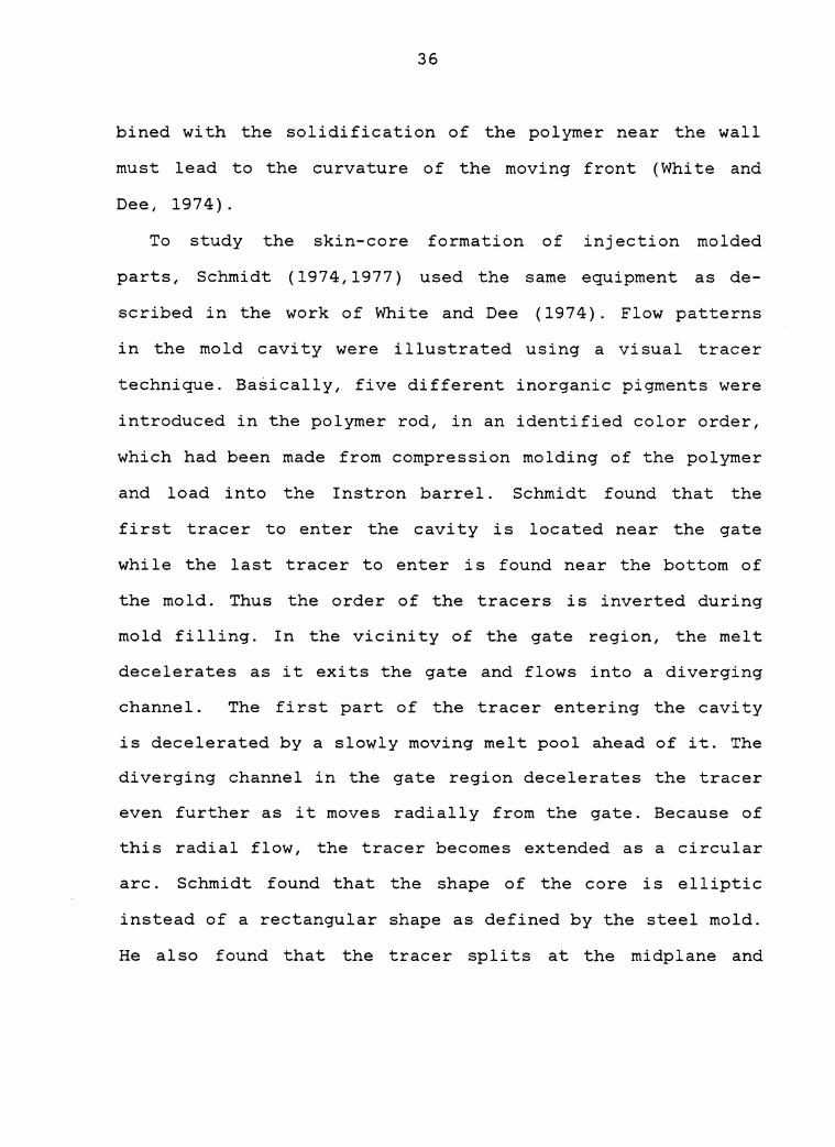
To study the skin-core formation of injection molded
parts, Schmidt (1974,1977) used the same equipment as de-
scribed in the work of White and Dee (1974). Flow patterns
in the mold cavity were illustrated using a visual tracer
technique. Basically, five different inorganic pigments were
introduced in the polymer rod, in an identified color order,
which had been made from compression molding of the polymer
and load into the Instron barrel. Schmidt found that the
first tracer to enter the cavity is located near the gate
while the last tracer to enter is found near the bottom of
the mold. Thus the order of the tracers is inverted during
mold filling. In the vicinity of the gate region, the melt
decelerates as it exits the gate and flows into a diverging
channel. The first part of the tracer entering the cavity
is decelerated by a slowly moving melt pool ahead of it. The
diverging channel in the gate region decelerates the tracer
even further as it moves radially from the gate. Because of
this radial flow, the tracer becomes extended as a circular
arc. Schmidt found that the shape of the core is elliptic
instead of a rectangular shape as defined by the steel mold.
He also found that the tracer splits at the midplane and
37
this tracer is found on the front. This occurs probably be-
cause the flow front is continuously splitting. The split-
ting action adds an additional velocity component to the
velocity vector. Therefore, the trajectory of the midplane
tracer material is an arc from the midplane to the cavity
wall. This flow mechanism produces the molecular orientation
as reviewed in the previous section.
As discussed previously, the flow of the polymer melt in
the entrance region is classified as radial flow. Kamal and
Kenig (1972) proposed a model for this type of flow. In this
work, these authors used a semicircular mold as shown in
figure 2.3.1.c. This mold was chosen in order to study ra-
dial flow without the interference from the wall of the
mold. The model is based on setting up the equation of con-
tinuity, motion and energy for the system during each of the
stages of the injection molding cycle i.e. filling, packing
and cooling. Using numerical techniques, they were able to
solve for the flow rate, velocity profiles at different
times and front positions in the cavity, and the progression
of the melt front.
The radial flow in which the melt is fed at the center of
the mold (figure 2.3.1.d) has also been studied by many au-
thors (Berger and Gogos, 1973; Wu, Hwang, and Gogos, 1974;
Laurencena and Williams, 1974; Winter, 1975; Schmidt, 1976).
38
Berger and Gogos (1973) and Wu et al. (1974) used the gener-
al transport equations, i.e. continuity, momentum and energy
equations to solve the transient and non-isothermal problem
of filling a disc-shape cavity with poly (vinyl chloride).
From this result, these authors predict pressure gradients,
fi 11 time and short shots. Furthermore, the velocity and
temperature fields were obtained throughout the formation of
a frozen surface layer during filling.
Following the work of Berger and Gogos and Wu et al. ,
Winter (1975) conducted a similar investigation but included
poly (ethylene) and polystyrene. He chose to modify the pow-
er-law model to include the normal stress components and
used in this model to predict pressure gradients and normal
stress distribution. The computed result differ by about 20
percent with the experimental pressure profiles.
In all of the work involving_ radial flow discussed so far
the flow at the entry region has been ignored. All of these
investigators obtained numerical solutions to the equations
of continuity, motion and energy based on a power-law const-
itutive relationship. From the numerical solution, they com-
puted temperature and pressure gradients, velocity profiles,
and the position of the advancing front as a function of
time. The inlet effects due to the stagnation flow were also
assumed negligible, and the solution started at a point bey-
ond this stagnation region.

39
Schmidt (1976) studied both the stagnation flow and
diverging radial flow between the parallel plates. He used
pigmented fluid elements as tracers to illustrate the flow
patterns which were recorded on a movie film. The data taken
from this movie film served as a basis to measure the veloc-
ity of the fluid elements as a function of both time and
distance. He found that the complex entrance region associ-
ated with stagnation flow leading to diverging radial flow
between parallel plates is large and of the order of 5 to 10
times the plates seperation. The flow in this region is a
combination of extensional flow and shear flow resulting
from the rearrangement of the velocity profile. Beyond the
entrance region, the flow is less complicated and can be de-
scribed as a combination of plannar extension and simple
shear flow.
40
!
---
(a) (b)
0 (c) (d)
Figure 2.3.1 Mold Filling Patterns in Different Geometry

Rffi!ON 3
GATE ENTRANCE ' \
\ I
I I
/ ,,.
.F'LOW DIRECTION FLOW FRONT
Figure 2.3.2 Mold Filling Characteristics in Rectangular Cavity
42
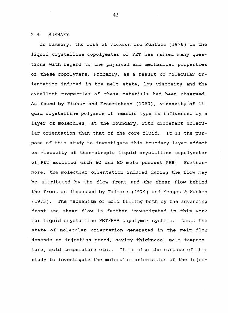
2.4 SUMMARY
In summary, the work of Jackson and Kuhfuss (1976) on the
liquid crystalline copolyester of PET has raised many ques-
tions with regard to the physical and mechanical properties
of these copolymers. Probably, as a result of molecular or-
ientation induced in the melt state, low viscosity and the
excellent properties of these materials had been observed.
As found by Fisher and Fredrickson (1969), viscosity of li-
quid crystalline polymers of nematic type is influenced by a
layer of molecules, at the boundary, with different molecu-
lar orientation than that of the core fluid. It is the pur-
pose of this study to investigate this boundary layer effect
on viscosity of thermotropic liquid crystalline copolyester
of~ PET modified with 60 and 80 mole percent PHB. Further-
more, the molecular orientation induced during the flow may
be attributed by the flow front and the shear flow behind
the front as discussed by Tadmore (1974) and Menges & Wubken
(1973). The mechanism of mold filling both by the advancing
front and shear flow is further investigated in this work
for liquid crystalline PET/PHB copolymer systems. Last, the
state of molecular orientation generated in the melt flow
depends on injection speed, cavity thickness, melt tempera-
ture, mold temperature etc.. It is also the purpose of this
study to investigate the molecular orientation of the injec-

43
tion molded parts under different molding condition by mea-
suring at the shrinkage of their microtomed samples.
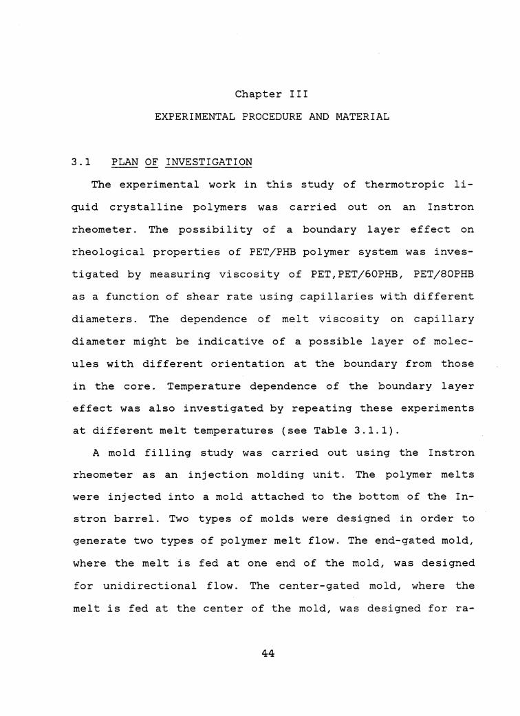
Chapter III
EXPERIMENTAL PROCEDURE AND MATERIAL
3.1 PLAN OF INVESTIGATION
The experimental work in this study of thermotropic li-
quid crystalline polymers was carried out on an Instron
rheometer. The possibility of a boundary layer effect on
rheological properties of PET/PHB polymer system was inves-
tigated by measuring viscosity of PET,PET/60PHB, PET/80PHB
as a function of shear rate using capillaries with different
diameters. The dependence of melt viscosity on capillary
diameter might be indicative of a possible layer of molec-
ules with different orientation at the boundary from those
in the core. Temperature dependence of the boundary layer
effect was also investigated by repeating these experiments
at different melt temperatures (see Table 3.1.1).
A mold filling study was carried out using the Instron
rheometer as an injection molding unit. The polymer melts
were injected into a mold attached to the bottom of the In-
stron barrel. Two types of molds were designed in order to
generate two types of polymer melt flow. The end-gated mold,
where the melt is fed at one end of the mold, was designed
for unidirectional flow. The center-gated mold, where the
melt is fed at the center of the mold, was designed for ra-
44

45
dial flow. The purpose of having the center-gated mold is to
make an attemp to generate biaxial orientation. Flow visual-
ization was accomplished by introducing different color pig-
ments into the melt and using a TV camera to record the
movements of these colored pigments through glass windows in
the mold. The mechanism of the melt filling the cavity was
investigated by making short-shots in which the fluid par-
tially fills the cavity. Finally, the molecular orientation
in these flows, i.e. radial and unidirectional flows, was
qualitatively studied by measuring the shrinkage of the mi-
crotomed samples.
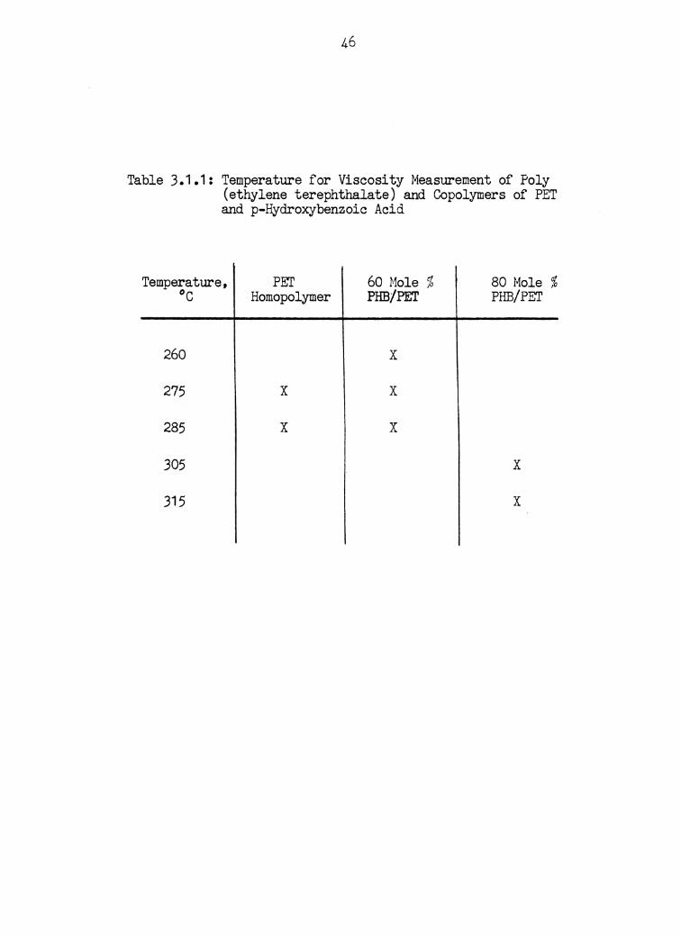
Table 3.1.1: Temperature for Viscosity Measurement of Poly (ethylene terephthalate) and Copolymers of PET and p-Hydroxybenzoic Acid
Temperature, PEI' 0 c Homopolymer
260
275 x
285 x
305
315
60 Mole % PHB/P'.ET
x
x
x
80 Mole % PHB/PET
x
x
47
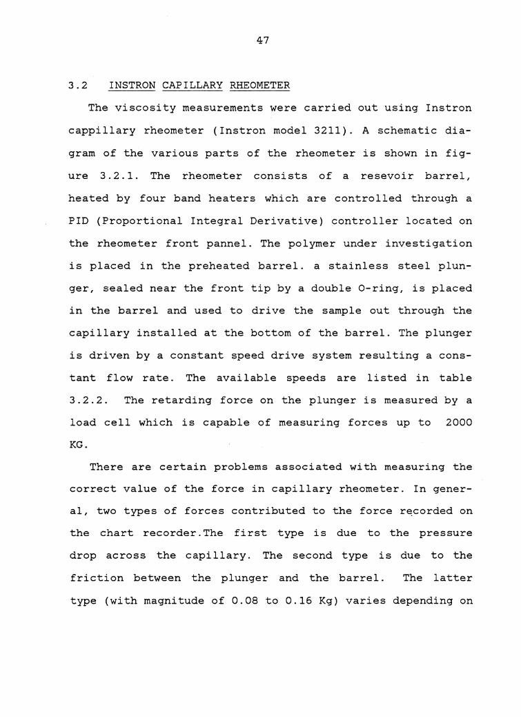
3.2 INSTRON CAPILLARY RHEOMETER
The viscosity measurements were carried out using Instron
cappillary rheometer (Instron model 3211). A schematic dia-
gram of the various parts of the rheometer is shown in fig-
ure 3. 2. 1. The rheometer consists of a resevoir barrel,
heated by four band heaters which are controlled through a
PID (Proportional Integral Derivative) controller located on
the rheometer front pannel. The polymer under investigation
is placed in the preheated barrel. a stainless steel plun-
ger, sealed near the front tip by a double 0-ring, is placed
in the barrel and used to drive the sample out through the
capillary installed at the bottom of the barrel. The plunger
is driven by a constant speed drive system resulting a cons-
tant flow rate. The available speeds are listed in table
3.2.2. The retarding force on the plunger is measured by a
load cell which is capable of measuring forces up to 2000
KG.
There are certain problems associated with measuring the
correct value of the force in capillary rheometer. In gener-
al, two types of forces contributed to the force r~corded on
the chart recorder. The first type is due to the pressure
drop across the capillary. The second type is due to the
friction between the plunger and the barrel. The latter
type (with magnitude of 0.08 to 0.16 Kg) varies depending on

48
the position of the plunger in the barrel (the amount of
contact between the plunger and the barrel). In measuring
low forces as in the case of the polymer involved in this
study, this friction force becomes a serious problem. To ob-
tain a repeatable value, the Instron barrel was half-filled
with polymer and care was taken to record the values of the
force at the same position of the plunger for every run.

49
INSULATION
~--;-,._HEATERS
r----+-1- CAPILLARY
---RETAINING RING
Figure 3.2.1: Schematic Diagram of Instron Capillary Rheometer (Jerman, 1980)

50
TABLE 3.2.i
Gear Ratio and Speeds For Instron Model 3211 Capillary Rheometer
(Cm/Min)
Gear Ratio
1 :1 1:2 2:1
o.06 0.03 0.12 0.20 0.10 0.40 0.60 0.30 1.20 2.00 1.00 4.00 6.oo 3.00 12.0 20.0 10.0 40.0
51
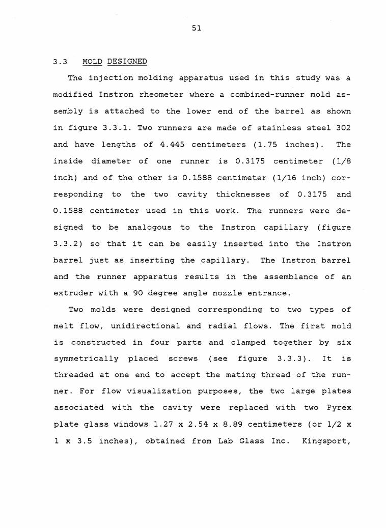
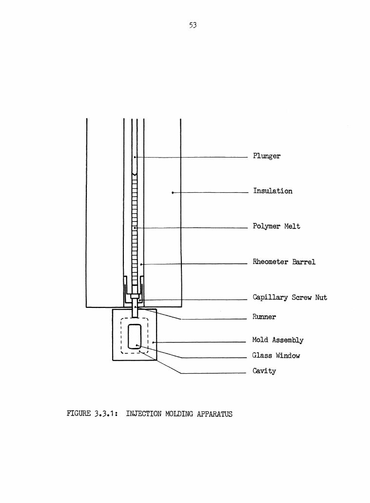
3.3 MOLD DESIGNED
The injection molding apparatus used in this study was a
modified Instron rheometer where a combined-runner mold as-
sembly is attached to the lower end of the barrel as shown
in figure 3.3.1. Two runners are made of stainless steel 302
and have lengths of 4. 445 centimeters ( 1. 75 inches). The
inside diameter of one runner is 0.3175 centimeter (1/8
inch) and of the other is 0.1588 centimeter (1/16 inch) cor-
responding to the two cavity thicknesses of 0.3175 and
0. 1588 centimeter used in this work. The runners were de-
signed to be analogous to the Instron capillary (figure
3. 3. 2) so that it can be easily inserted into the Instron
barrel just as inserting the capillary. The Instron barrel
and the runner apparatus results in the as semblance of an
extruder with a 90 degree angle nozzle entrance.
Two molds were designed corresponding to two types of
melt flow, unidirectional and radial flows. The first mold
is constructed in four parts and clamped together by six
symmetrically placed screws (see figure 3.3.3). It is
threaded at one end to accept the mating thread of the run-
ner. For flow visualization purposes, the two large plates
associated with the cavity were replaced with two Pyrex
plate glass windows 1.27 x 2.54 x 8.89 centimeters (or 1/2 x
1 x 3. 5 inches), obtained from Lab Glass Inc. Kingsport,

52
Tennessee. The cavity thickness can be changed by changing
the spacing between the two large surfaces of the mold. The
cavity is rectangular in shape and has a dimension of 2.54 x
8.89 x 0.3715 (or 0.1588) centimeters. The mold temperature
was controlled by four 150 watts catridge heaters connected
in parallel to an Omega model 4001 controller. The heaters
were inserted in holes drilled on the wall of the mold and
perpendicular to the large surface. An Iron-Constantan ther-
mocouple was placed near the top of the mold. In this way,
the mold temperature is always kept within ±1°C from the set
point. The temperature variation over the mold surface was
checked by means of a thermocouple attached at the bottom of
the mold. It had been observed that no temperature gradient
existed over this large surface of the mold.
The second mold was designed for radial flow. Basically,
it is same as the first mold except its size and the posi-
tion of the ·gate entrance. This mold has a dimension of
10.16 x 10.16 x 4.445 centimeters (or 4 x 4 x 1 .. 75 inches.
Instead of being end-gated, it has a threaded hole at the
center of the large surface to accept the mating thread of
the runner (see figure 3.3.4). Because of this position of
the runner, this mold is called center-gated mold.
53
~ ..... ..... ..... ..... . ..... I-..... ..... .... -.... -.... .... ..... -..... ..... .... ..... -..... ....
. .... . ~ ... -.... -r--._
~-... -,
I - I I I I I I I I
--~ · - - r--._ "---~-
FIGURE 3.3.1: INJECTION MOLDING APPARATUS
Plunger
Insulation
Polymer Melt
Rheometer Barrel
Capillary Screw Nut
Rtmner
Mold Assembly
Glass Window
Cavity
54
+ 0. ?>
//
_.____-t 0. 185"
t.5o"
0.38 Fine Thread
FIGURE 3.3.2: RUNNER

55
Figure 3. 3. 3: Photograph of Recta.."1.gular Mold

56
77
Fi.gure 3.3.4: PhotofSraph of Circular :fold
57
3.4 SAMPLE PREPARATION
The polymers used in this study are poly (ethylene ter-
ephthalate) and two copolyesters of PET, 60 and 80 mole %
p-hydroxybenzoic acid. The PET homopolymer is milky white
with glossy surface. The 60 mole percent pellets are an off
white with a soft sheen. The 80 mole percent pellet is beige
color wi;th rough appearance. All three polymers were pre-
pared and supplied by Tennesse Eastman Laboratories at
Kingsport, Tennesse.
According to Jackson and Kuhfuss (1976), the flow behav-
ior of these polymers is a function of temperature, shear
rate, and moisture content. Due to the chemical structure of
this polymer system, care had to be taken to avoid the pres-
ence of water or moisture during the experiments. This ne-
cessitated a carefull drying and special loading techniques.
Polyester such as PET is extremely hygroscopic (Van Der
Wielen, 1976) and the polymer will undergo a degradation in
the presence of moisture, resulting in a decrease in molecu-
lar weight and consequently, a decrease in viscosity (Wiss-
brun, 1979).
In this work, polymer pellets were stored in small glass
containers (28.3 ml) with sealable lids. The specimens were
placed in a vacuum oven and dried at a temperature of 110°c
and under a vacuum of 63. 5 centimeters of mercury for 72
58
hours. At the end of the drying time, the pressure of the
oven was returned to atmospheric pressure by bleeding in
prepurified nitrogen. On reaching atmosheric pressure, the
glass containers were covered, sealed using electrical tape
and allowed to cool to room temperature. All of these con-
tainers were then kept in a dessicator.
During each loading of polymer into the Instron barrel,
care was taken to retain as much of inert atmosphere as pos-
sible. A prepurified nitrogen line was connected to flow
downward into the rheometer barrel. This would displace the
moist air in the barrel. A small amount of polymer pellets
was rapidly fed into the barrel with the nitrogen still
flowing. The polymer was then tamped down to remove any
trapped gas bubles as the polymer melted. This process of
loading was repeated until the barrel had been half-filled
with polymer. The plunger was
slight pressure was applied,
then put in position and a
sealing the polymer from the
surrounding atmoshere as it was allowed to reach the running
temperature.

59
3.5 SAMPLE PREPARATION FOR FLOW VISUALIZATION STUDIES --- ---POLYMER ROD
For the visual tracer technique, five different colors of
pigmented polymers were placed into the polymer melt column
in the rheometer barrel. This was accomplished by inserting
these pigments into a precompression-molded polymer rod. The
rod is then fed into the rheometer from the bottom. In this
experiment, the polymer rod was prepared using the Instron
plunger-barrel as a compression unit. First, the barrel was
preheated to a compression molding temperature. This temp-
erature was chosen to be different depending on the type of
polymer (see Table 3. 5. 1). The bottom of the barrel was
blocked with a small disk which was held in place by the ca-
pillary screw nut. A small amount of polymer pellets was fed
into the barrel. The polymer was then compressed by the
plunger to a pressure of 1. 4 x 10 7 N/M 2 . Th f e process o
loading small amounts of pellets and compression was repeat-
ed until the barrel had been completely filled. At this
time, the barrel was allowed to cool down to a "cooling
temperature" to solidify the polymer inside the barrel. To
get the polymer rod out of the Instron barrel without using
a great amount of force, the temperature of the barrel was
slightly raised to a higher temperature. The rod was then
pushed out by means of the plunger.

60
To insert the pigmented polymer into the polymer rod,
five small holes were drilled partially through the rod,
perpendicular to the axis of symmetry. Pigmented polymer
pellets were inserted into these holes and plugged with the
original unpigmented polymer. The polymer rod was then fed
into the hot rheometer barrel.

Type of Polymer
PET Homopolymer
60 Mole % PHB/PET
80 Mole % PHB/PET
61
TABLE 3.5.1
Compression Holding Temperature for PET and its Copolymer with PHB
Compression Temperature,°C
230
220
270
Extrusion Temperature,°C
200
180
220
62
3.6 INJECTION MOLDING
In this experiment, the runner was held in place at the
bottom of the Instron barrel by the capillary screw nut. The
polymer pellets were then loaded using the same technique
discussed in section 3.4. At this time, the polymer was al-
lowed to reach the injection temperature before the mold as-
sembly was attached. During this heat-up period, a small
steel plug was placed in the runner to prevent the melt from
flowing down under the influence of the gravity. The plug
was quickly removed just before the mold assembly was at-
tached at ~he end of the runner. The mold was preheated by
four catridge heaters to an appropriate temperature. Final-
ly, the material was injected into the mold cavity at a
constant flow rate of 0.2375(10-4 ) and 0.475(10-4 ) cubic me-
ters per second. Similar experiments were run for a variety
of conditions. A summary of these conditions is shown in Ta-
ble 3.6.1
For short-shot type of injection, the same procedure de-
scribed above was used except that the polymer rod was fed
into the rheometer barrel from the bottom before the runner
was placed at the end of the barrel. The injection step was
stopped when the second fluid pigment showed up on the wall
of the cavity. This color can be seen through the glass win-
dow of the mold. The short-shot injected plaque was then cut
63
along to the flow direction and the photographs of these
sections were taken.
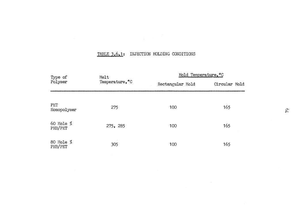
Type of Polymer
PET Homopolymer
60 Mole % PHB/PET
80 Mole % PHB/PET
TABLE 3.6.1: INJECTION MOLDit\lG CONDITIONS
Melt Temperature,°C
275
275, 285
305
Mold Temperature,°C
Rectangular Mold Circular Mold
100 165
100 165
100 165
O" .p-..

65
3.7 SHRINKAGE MEASUREMENT
Melt flow during the molding of injection molded parts
always causes an orientation of macromolecules along the
flow direction. This orientation significantly influences
the properties of the molded parts. To qualitatively study
the macromolecular orientation development of the molded
parts, a small sample of the molded plaque was cut and mi-
crotomed. The geometry and dimension of this cut are shown
in figure 3. 7 .1 for both rectangular and circular plaque.
This sample was microtomed using the Spencer 860 sliding mi-
crotome machine. The thickness of the microtomed specimen is -5 approximately 2.54(10 ) meter. The dimension of each of
these specimens was measured using a caliper. The thickness
was measured using a micrometer. From these thicknesses,
the distance from surface of each microtomed sample was det-
ermined. These samples were then heated in the oven above
their softening temperatures. These temperatures and the
heating times for different polymers are shown in Table
3.7.1. Finally, the dimension of the annealed samples was
remeasured and the percent shrinkage was calculated.

66
(a) Rectangular Plaque
~ o. 2"
(b) Circular Plaque
Figure 3.7.1: Dimension of Sample Cut From Injection Molded Parts

'fype of Polymer
60 Mole % PHB/PRI'
80 Mole % PHB/PET
67
TABLE 3.7.1
Annealing Time and Temperature for Shrinkage Measurement
Annealing Time, Min.
10
10
Annealing Temp., °C
200
260

4.1 CAPILLARY RHEOMETRY
Chapter IV
RESULTS
From the force and plunger speed data of the Instron ca-
pillary rheometer, viscosity of poly (ethylene terephtha-
late) and its copolyesters with 60 and 80 mole % p-hydroxy-
benzoic acid were determined. First, the graphs of total
pressure drop, !:::.. P, versus the apparent shear rate, 'kAP? ,
were contructed. Examples for this type of graphs are shown
in figure 4. 1. 1 to 4. 1. 3. Pressures at constant apparent
shear rates were taken from these graphs and plotted against
the capillary length to diameter ratio, L/D. This type of
plot is commonly called a Bagley plot. The lines of the Bag-
ley plot appear to be nearly linear and were fit into a line
least squares program. From this program, the intercepts of
these lines with the ordinate give the end pressures (in-
cluding entrance pressure loss and exit residual pressure)
for various shear rates. In general, the exit residual
pressure is small and the end pressure can be assumed as
entrance pressure loss (Han, 1976). Typical examples of
Bagley plots corresponding to figure 4. 1. 1 to 4. 1. 3 are
shown in figure 4.1.4 to 4.1.6. Figures 4.1.7 to 4.1.9 show
the results of entrance pressure loss, /:J. Pen , as a function
68
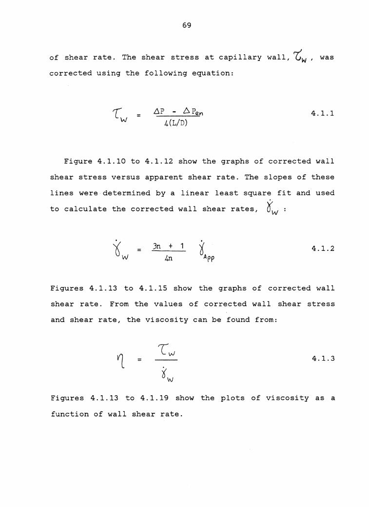
69
of shear rate. The shear stress at capillary wall, t:w , was
corrected using the following equation:
fl? - 6 PeY\ 4(1/D)
4.1.1
Figure 4.1.10 to 4.1.12 show the graphs of corrected wall
shear stress versus apparent shear rate. The slopes of these
lines were determined by a linear least square fit and used
to calculate the corrected wall shear rates, Ow :
. (;'w =
Jn + 1
4n i App
4.1.2
Figures 4.1.13 to 4.1.15 show the graphs of corrected wall
shear rate. From the values of corrected wall shear stress
and shear rate, the viscosity can be found from:
= 4 .1. 3
Figures 4 .1. 13 to 4. 1. 19 show the plots of viscosity as a
function of wall shear rate.

70
Throughout the viscosity measurement a fortran program
was used based on the above outline. A copy of this program
is shown in appendix A.
The results of these calculations are presented in tabu-
lar form in appendices B-1 through B-3 Values of raw
data, apparent and wall shear rates, corected wall shear
stresses, melt viscosities and entrance pressure losses are
given.
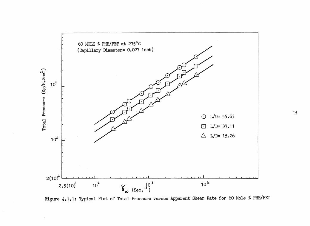
-c-J • () Q)
Cl) • :::
...........
~ ........ Q)
~ f/l f/l Q)
J::
~ E-t
106
105
60 MOLE % PHB/PET at 275°C (Capillary Diameter= 0.027 inch)
0 L/D= 55.63
0 L/D= 37.11
6 L/D= 15.26
2(1of '---L-__.___._.___.__.__._._~_.___._-L---l-L-L.JL.L.L.~--'~_._..J__l__J___j~.L_~_J___L__._-'--'--LL~ 2.5(10)1 102. . 10 3
'(w (Sec.-• ) 1oir
Figtn'e 4.1.1: Typical Plot of Total Presstn'e versus Apparent Shear Rate for 60 Mole% PHB/PET
-.J __.
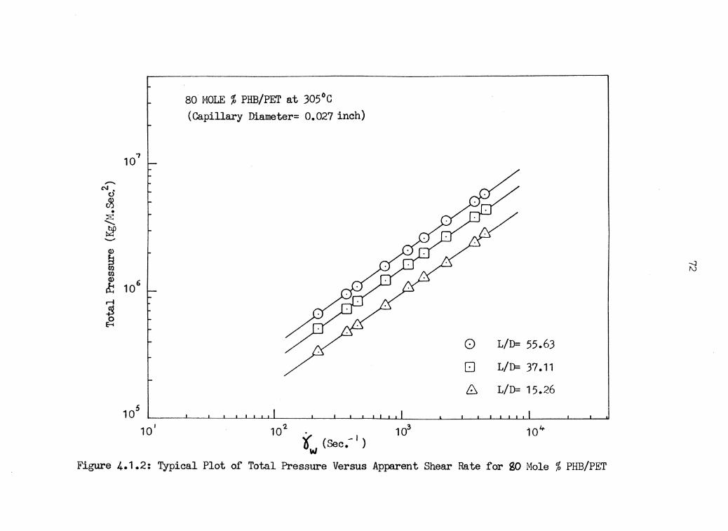
107
-"' . 0
r93 • ~ .......... ~ .......... Q)
~ (Q (Q Q)
106 ~ r-1
~ E-t
105
10'
80MOLE % PHB/PET at 305°C (Capillary Diameter= 0.027 inch)
102 i. (Sec.- 1 ) w 103
0 L/D= 55.63
8 L/D= 37.11
b L/D= 15.26
10""
Figure 4.1.2: Typical Plot of Total Pressure Versus Apparent Shear Rate for go Mole % PHB/PET
-J l\J
.......... ...a.
()
~ • ~
.......... ~ .......... Q) a (/) (/) Q)
~
~ ~
107
10b
PET HOMOPOLYMER at 285°C (Capillary Diameter= 0.027 inch)
c::J L/D= 55.63
0 L/D= 37.11
0 L/D= 15.26
2(1of ..._._~_._~_._.......~~_.__.__._-'--'L._L_Jl-Li.~~-'---L--L--L-JL--L-l--'--L~~J.._--'--'---L.....l---'-'....L.I 2.5(10)1 10 2. 3 . 10 I 15-w (Sec.- )
104-
Figure 4.1.3: Typical Plot of Total Pressure Versus Apparent Shear Rate for PET Homopolymer
-..J VJ
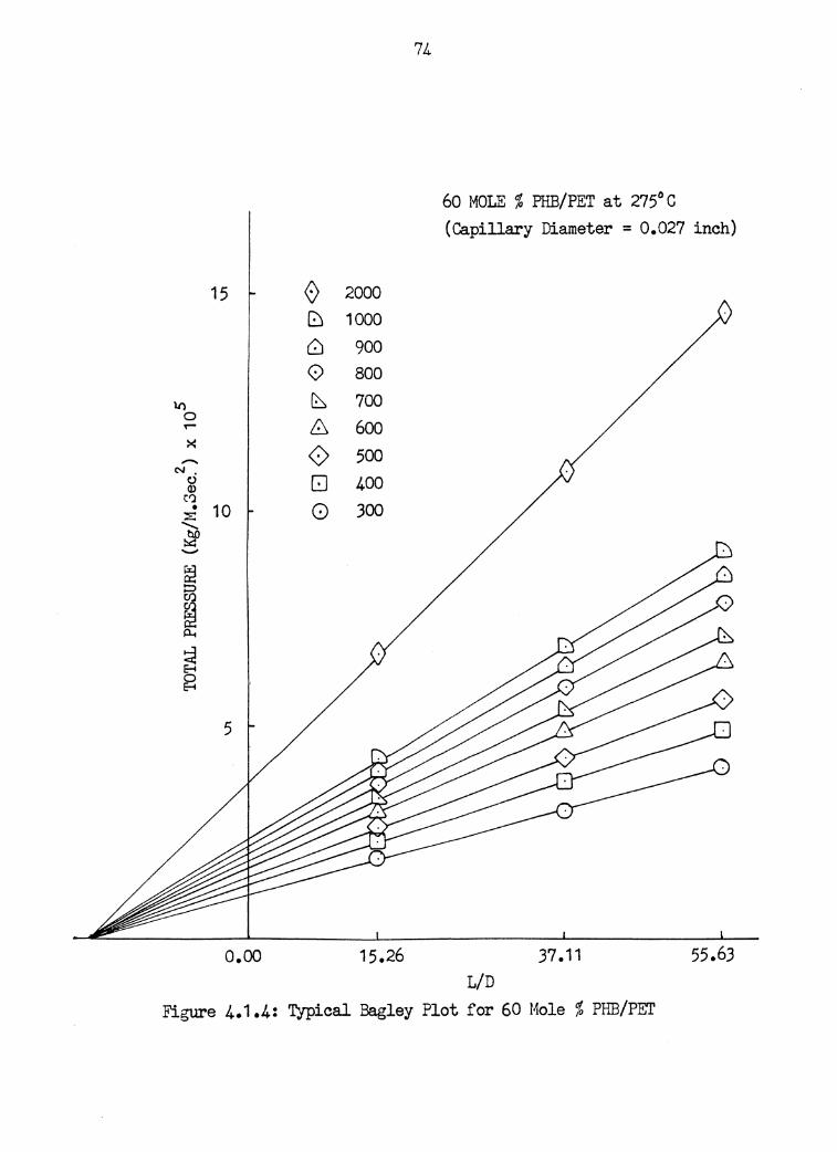
74
60 MOLE % PHB/PET at 275°C (Capillary Diameter = 0.027 inch)
15 0 2000 ~ 1000 ~ 900 0 800
\/) ~ 700 0 (;:::, ,..- 600 >< 0 ........ 500
N, Q GJ 400 Q>
C') • 10 0 300 ~ ............
~ ..........
~ ~ ~ p..,
~ 0 E-t
5
o.oo 15.26 37.11 55.63 L/D
Figure 4.1.4: Typical Bagley Plot for 60 Mole % PHB/PET

30
\0 0 ..-><
........ c-a •
0 ID
(/) • :<::
...........
~ 20 -~ ~ p...
~
o.oo
0 tJ ~ 0 ~
0:,
0 8 0
2000 1000
900 800 700 600 500 400 300
15.26
75
80 MOLE % PHB/PET at 305°C (Capillary Diameter = 0.027 inch)
37.11 55.63 L/D
Figure 4.1.5: Typical Pagley Plot for 80 Mole % PHB/PET
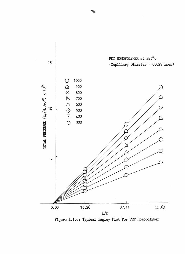
15
..$) 0 ,.... ::< -"'· () (1)
U,l • 10 ::::;:: ...........
~ -~ §3 ~ p...
~ 0 E-1
5
o.oo
0 ~ 0 ~
8 0 [!]
0
1000 900 800 700 600 500 400 300
15.26
76
L/D
PET HOMOPOLYMER at 285°C (Capillary Diameter = 0.027 inch)
37.11 55.63
Figure 4.1.6: Typical Bagley Plot for PEI' Homopolymer

Figure 4.1.7:
60 MOLE % PHB/PET at 275°C (Capillary Diameter = 0.027 inch)
102 103 10"' 105" "i(APP (Sec .-1 )
Entrance Pressure Loss versus Apparent Shear Rate for 60 Mole % PHB/PET
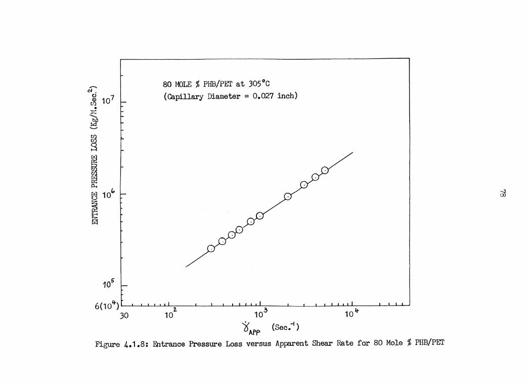
.......... "' . ~ 107 • ::?.:: .........
M ~ ......... Cl) Cl)
8
~ ~ fl...
~ 10'1
~ ~
80 MOLE % PHB/PET at 305°C (Capillary Diameter = 0.027 inch)
6(10*)~L-J..--'--.j~-'-;;-~~----L~L__L-L-L-L.L.l~~--L~-L--1-L...L..LLLL~___!_l_--1.....1....J 30 10 1 o3 10 lf-
y _, o APP (Sec. )
Figure 4.1.8: Entrance Pressure Loss versus Apparent Shear Rate for 80 Mole % PHB/PET
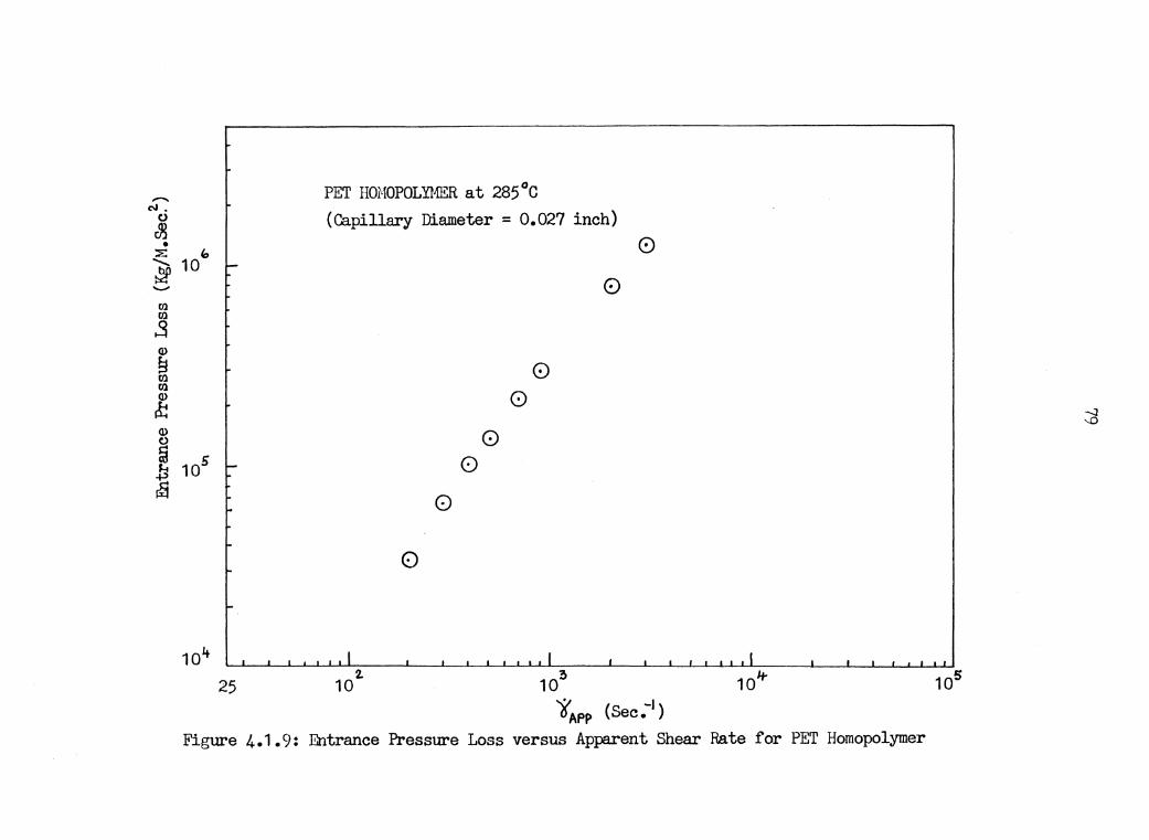
"""' cl • ()
~ • ::?.: ...........
~ ..._., Cl) Cl) .s Q) s Cl) Cl) Q)
~ Q) ()
§ _fj iS
" 10
105
PET HOHOPOLYMER at 285°C (Capillary Diameter = 0.027 inch)
0
0
0 0
0
0
0
103
0
1APP (Sec.-1) Figure 4.1.9: Entrance Pressure Loss versus Apparent Shear Rate for PET Homopolymer
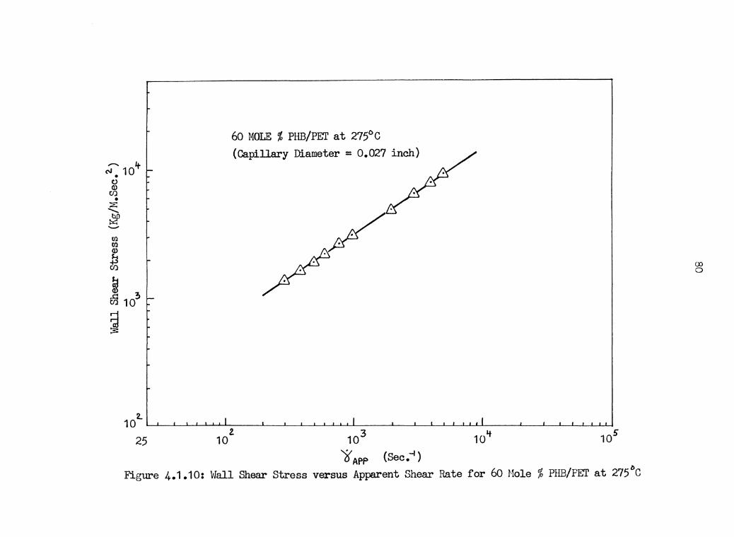
60 MOLE % PHB/PET at 275°C (Capillary Diameter = 0.027 inch)
/ /
103
'j{ APP (Sec.-1) 10't
Figure 4.1.10: Wall Shear Stress versus Apparent Shear Rate for 60 Mole% PHB/PET at 275t>C
00 0

-cJ • (.)
~101+ ~
.......... ~ ........ (/) (/) Q)
b Cl)
fd Q)
61 ~ 10 !>
200 25
80 ;,10LE % PHB/PET at 305°C (Capillary Diameter = 0.02? inch)
2.. 10 10 3
".:./ I 0 APP (Sec.- )
101.t
Figure 4.1.11: Wall Shear Stress versus Apparent Shear Rate for 80 Mole% PHB/PET at 305°C
co ~
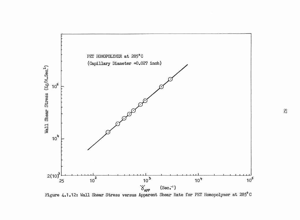
PET HOMOPOLYMER at 285°C
- (Capillary Diameter =0.027 inch) <"I •
0 Q)
ti) • ::E: .........
105 ~ .._.. (I) (I) Q)
_f3 ti)
m 83 r-l
~ 101+
2(1of ,_.___.__..__,'--'---'~~~____.~__.___.___,.___._-'--'-'L-L--~-'---JL-JL...-L-L-l_i_J__J-_~_.____.___.__J__J_j_~ 25 10 103 101t 105
l5APP (Sec.-') Figure 4.1.12: Wall Shear Stress versus Apparent Shear Rate for PET Homopolymer at 285°C
CXl lV

~ t) Q)
U) • ~ t) I'll
~ .........
c'
10 1 -... ...
...
10° f-- 0 260°C c:J 275°C 0 285°C
60 MOLE % PHB/PET (Capillary Diameter = 0.027 In.)
-I I I I 10 ._.__,_1___,__.___.--'-'-_.__~_,_~_.__~1_._~,~·'-'-'--'-~---'-'~_.____.___.__. • ._._.._._.~~-·.___.__.__.__,_11_._.1_._.1
25 10 2. 10 ~ 10 It 1 o5
¥w (Sec:') Figure 4.1.13: Melt Viscosity as a Function of Wall Shear Rate for 60 Mole % PHB/PET with
Capillary Diameter of 0.027 inch
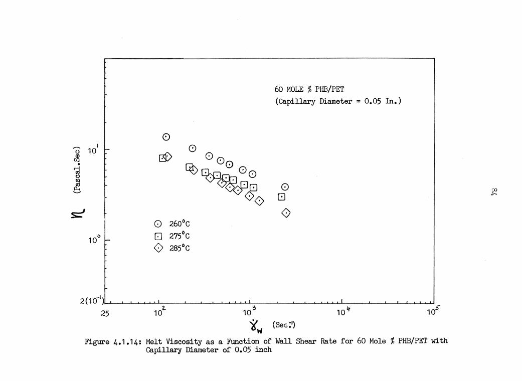
-0 Q)
Cl) •
'd 0 (J)
~ ....._...
I 10 -
0 260°C ['.] 275°C (> 285°C
60 MOLE % PHB/PET (Capillary Diameter= 0.05 In.)
0 G
0
2 ( 10-I ).__...___._-.1--~__._._..__ , _ __.__..___,__~-1-1.--L...L1 ----'-----L------'L.....-J..-'-.LJ_Ul------'--J.....__..J...• __L_-'--1.--L-1..J
25 1 oz. 10 "3 10 Lt v O, (SeG:1) ~
Figure 4.1.14: Melt Viscosity as a F\mction of Wall Shear Rate for 60 Mole % PHB/PET with Capillary Diameter of 0.05 inch

......,. 0 (1) I (/) 10 • -
M aj 0 (/) aj
p..,
s::.'
10° -
25
0 260°C c:J 275°C 0 285°C
• I I I
60 MOLE % PIIB/PET (Capillary Diameter = 0.070 In.)
I I I
103
~w (Sec:1)
l
10Lt
Figure 4.1.15: Melt Viscosity as a Function of Wall Shear Rate for 60 Mole% PHB/PET with Capillary Diameter of 0.07 inch
co '-"

----·
0 305°C
El 31s 0c
80 MOLE % PHB/PET (Capillary Diameter = 0.027 In.)
I I
10~
(Sec.-•)
Figure 4.1.16: Melt Viscosity as a Function of Wall Shear Rate for 80 Mole % PHB/PET with Capillary Diameter of 0.027 inch
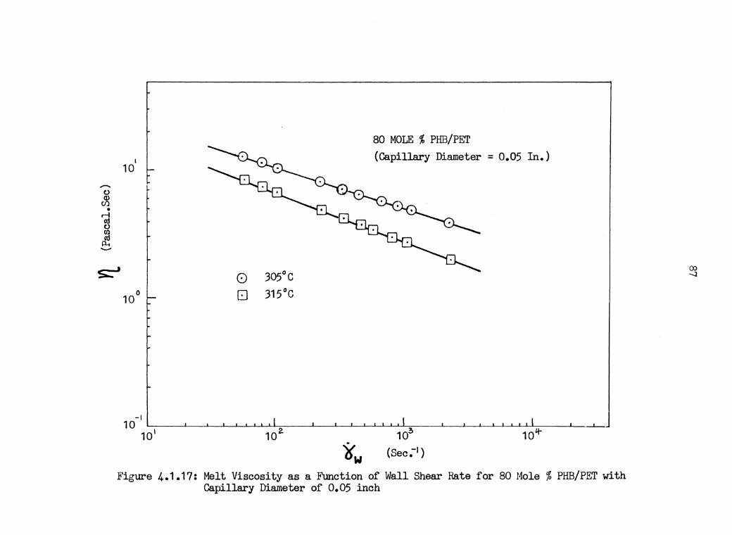
80 MOLE % PIIB/PET I (Capillary Diameter = 0.05 In.)
10 -() Q)
CJ) • ~ () Ul cd p_., .........
~ 0 305°C
10 0
-I 10
101
8 315°C
1oir
'if w Figure 4.1.17: Melt Viscosity as a Function of Wall Shear Rate for 80 Mole % PIIB/PET with
Capillary Diameter of 0.05 inch
00 .....J
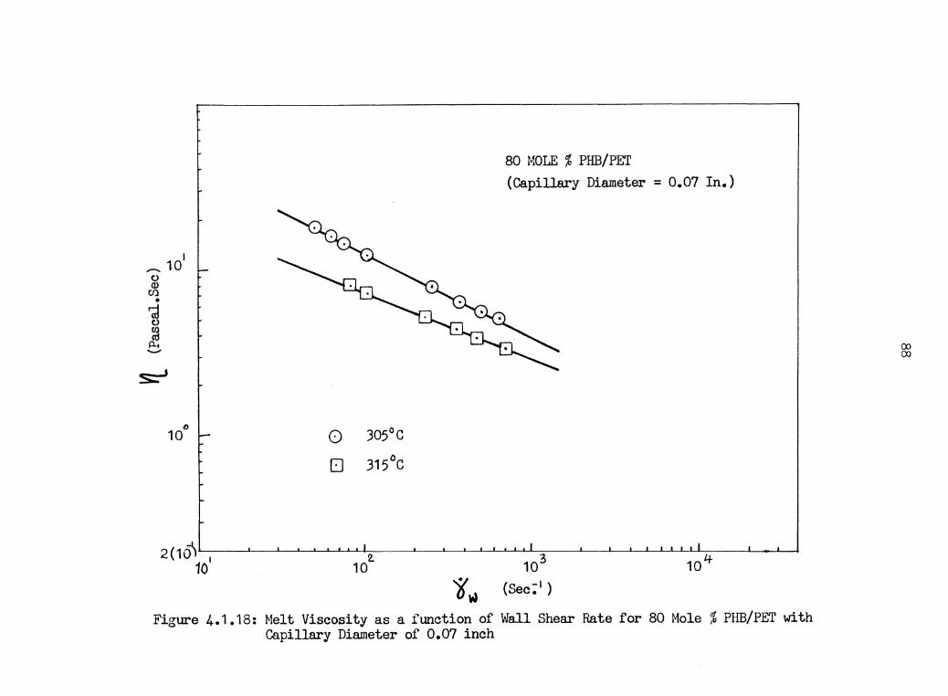
80 MOLE % PHB/PET (Capillary Diameter = 0.07 In.)
,,......, 10 I (.) Q)
(/) •
'cl (.) Ul cd
ri. .........
s:-'
t)
10 O 305°C
EJ 315°C
2(10\.__,~-L...~L-.l-1-L...-'--'-~~~---'~_L__L__J__j'-'-L'-1.~~_.____._--'--L-'-l_L.l_J_~-l.~..L-1
10 10 103 104-'i{ W (Sec: 1 )
Figlll'e 4.1.18: Melt Viscosity as a function of Wall Shear Rate for 80 Mole% PHB/PET with Capillary Diameter of 0.07 inch
co co

PET HOMOPOLYMER (Capillary Diameter = 0.027 In.)
2 ........ 10 (.)
~ • «1 (.) I'll
~ .......
s;-' ~ 275°C
I 0 285°C 10
2 101 103
'if w (Sec:1 )
Figure 4.1.19: Melt Viscosity as a Function of Wall Shear Rate for PET Homopolymer with Capillary Diameter of 0.027 inch
CXl
'°
90
4.2 MOLD FILLING CHARACTERISTICS
The investigation of mold filling characteristic of these
liquid crystalline polymer systems composes of two parts:
Flow visualization of color pigmented polymers and short-
shot type of injection. First, from the video tape recorded
during experiment, the distance of fluid pigments from gate
was plotted against the time of injection. Examples of this
plot for the flow visualization of PET are shown in figure
4.2.1 and 4.2.2. Figure 4.2.1 shows the data of these plots
of PET injected into a cold mold whereas figure 4.2.2 shows
a similar plot for injection into the hot mold. The slopes
of these data points on these curves
of the fluid pigments at that time.
represent the velocity
Figure 4.2.3 and 4.2.4
show the velocity of these pigments as a function of their
positions in the mold (distance from gate).
The flow visualization experiments described above only
show the movement of the pigmented polymers in two dimen-
sions: along the flow and across the flow direction. To see
the complete picture of the filling patterns of the melt
flow, one must see the filling pattern of these pigments in
the section perpendicular to the large surface of the melt
flow and parallel to the direction of flow. Figures 4.2.5
to 4.2.7 show the photographs of a short-shot type of injec-
tion for PET, PET/60PHB and PET/80PHB respectively. Lastly,

91
a photograph of a section transverve to the flow direction
and perpendicular to the large surface of the melt flow is
shown in figure 4.2.8.
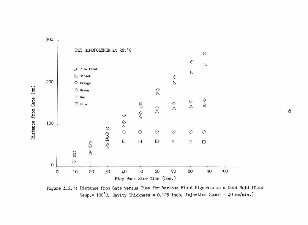
......... ~
'--"
$ ~ s 0 H
CH Q) t)
~ £Jl a
300
PET HOMOPOLYHER at 285°C 0
0 ~
0 Flow front b,
~ Violet 0 200 0 Orange b,
6 Green () b,
0Red 0 0
[J Blue ~ 0 ~ &
0 & 0 &
() & 100 ~
0 &
~ 0 <) 0 0 0 <)
8 Q [] [] Q [] [] G ~
8 f! 0 0
'------'--- ·-----0 10 20 30 40 50 60 70 80 90 1UU
Play I3ack Slow Time (Sec.)
Figure 4.2.1: Distance from Gate versus Time for Various Fluid Pigments in a Cold Mold (Mold Temp.= 100°C, Cavity Thiclmess = 0.125 inch, Injection Speed= 40 cm/min.)
,_Q I\)
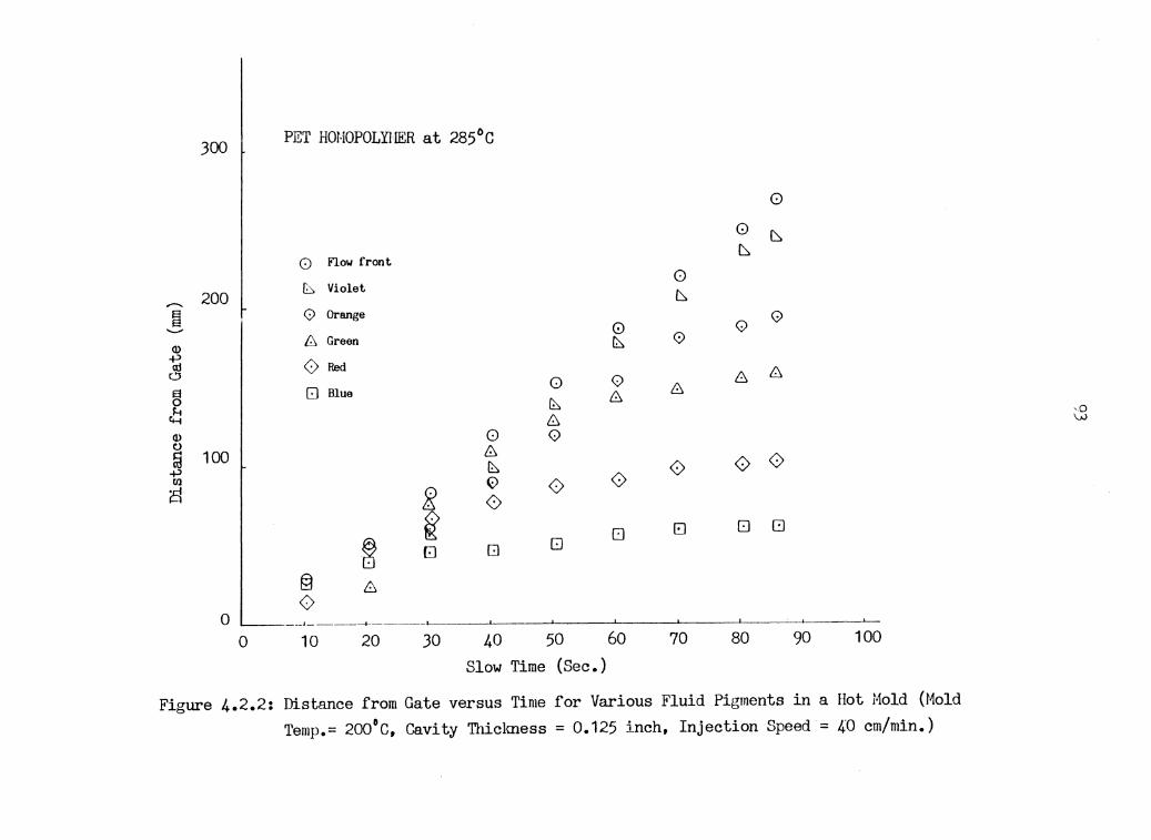
300 PET HOMOPOLYIIER at 285°C
8 Flow front
[;:::, Violet
0 Orange
8 Green
0Red (J Blue
jg ~ El
0 6 ~ 0 0
G
0 ~ 6 0
0
(J
0
0 ~ b.
0 b.
0 0 0 ~ 0
0 6 6 6 6
0 0 0 0
0 EJ (J G
0 ..___. __ , _____ __. _______ .___ _ ___._ __ ___. ___ ___._ __ ___._ __ ___._ __ -'----J. __ _
0 10 20 30 40 50 60 70 80 90 100 Slow Time (Sec.)
Figure 4.2.2: Distance from Gate versus Time for Various Fluid Pigments in a Hot Mold (Mold Temp.= 200°C, Cavity Thiclmess = 0.125 inch, Injection Speed = 40 cm/min.)
,0 'vJ
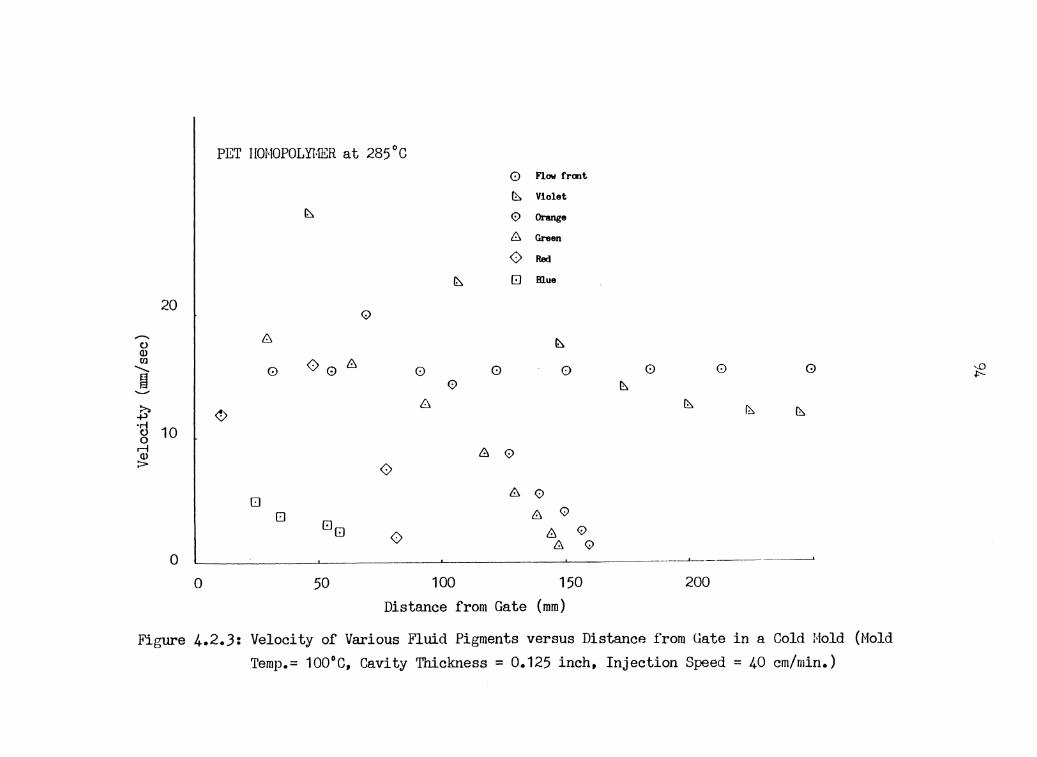
PET IIOMOPOLYHER at 285°C 0 Fl.ow frmt
~ Violet ~ 0 Orange
8 Green
0 Red
~ El filue
20 0
......... 6 ~ t) Q) Cll 00 8 .......... 0 0 0 0 0 0 0 ~ 0 !:::.
v 8 ~ ~ ~ ~ ·rl 10 t) 0 rl & 0 Q) :> 0
8 0 El El 8 0
El & 0 El 0 & 0 0 ____ ______.__, ________ ________.
0 50 100 150 200 Distance from Gate (mm)
Figure 4.2.3: Velocity of Various Fluid Pigments versus Distance from Gate in a Cold Mold (.Mold Temp.= 100°C, Cavity Thickness= 0.125 inch, Injection Speed= 40 cm/min.)
,_Q l'-
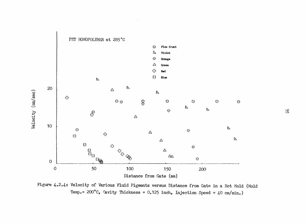
-() Q) rJl ......... ~ ~
$ •r-1 () 0 rl ~
PET HOHOPOLYMER at 285°C 0 now frcmt ~ Violet
0 Orange 8 Green
0 Red
~ EJ Blue
20 8 ~
~
0 00 ~ 0 0 0 0
~ ~
8 0 8
10 ~ 0 8 0 EJ 0
8 ~
EJ 0 0
0
EJ 0 8 EJ 0~ ~ EJ
0 .~ 0 50 100 150 200
Distance from Gate (mm)
Figure 4.2.4: Velocity of Various Fluid Pigments versus Distance from Gat~ in a Hot Mold (Mold Temp.= 200°C, ~,avity Thickness= 0.125 inch, Injection Speed= 40 cm/min.)
'° \J1
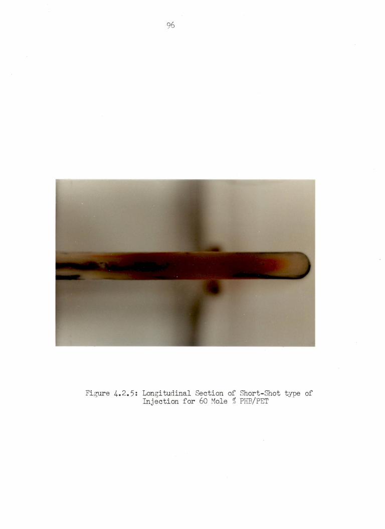
96
Figure 4.2.5: Longitudinal Section of Short-Shot type of Injection for 60 Mole % PHB/PET
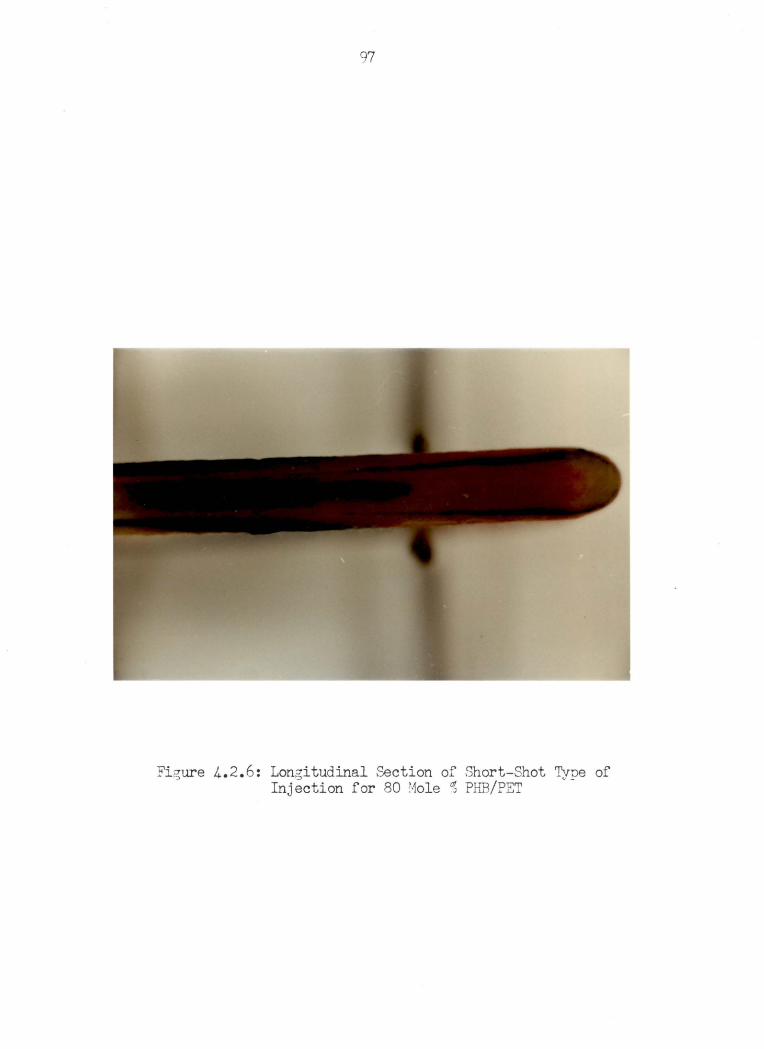
97
Fisure 4.2.6: Longitudinal Section of Short-Shot Type of Injection for 80 Mole ~ PHB/PET

98
Figure 4.2.7: Longitudinal Section of Short-Shot type of Injection for PET homopolymer
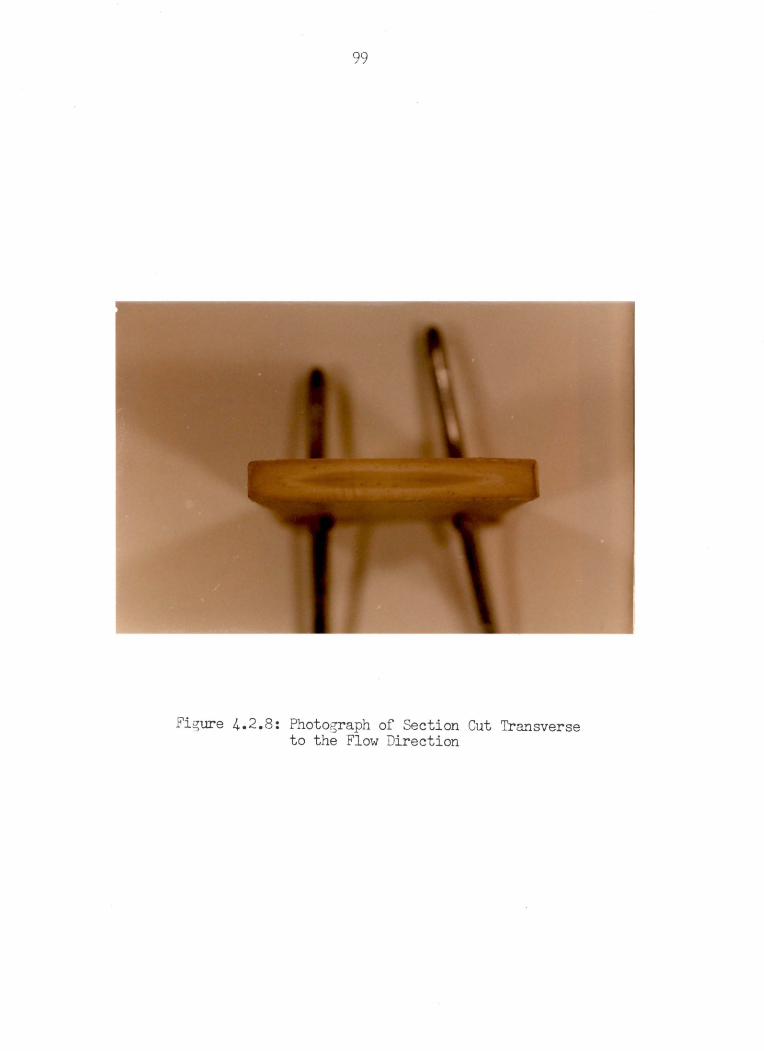
99
Figure 4.2.s: Photograph of Section Cut Transverse to the Flow Direction
100
4.3 SHRINKAGE MEASUREMENT OF MICROTOMED SAMPLES
Molecular orientation generated during the injection
molding of polymer melt influences significantly the proper-
ties of the molding.
face to the core of
This orientation varies from the sur-
the ~njection molded part. Since
shrinkage depends on this state of orientation, one method
to qualitatively rate the degree of orientation is to mea-
sure the shrinkage of the microtomed samples of the injec-
tion molded parts. The state of orientation depends on many
injection molded variables, i.e. speeds of injection, cavity
thicknesses, mold temperatures, type of melt flow. Conse-
quently, the degree of shrinkage will vary with these varia-
bles as well. In this section, the plots of the percent
shrinkage of microtomed samples versus the distance from the
surface of the molded parts are shown for various injection
molded conditions. Figures 4.3.1 to 4.3.12 show the shrink-
age measurement data for the injection molding of liquid
crystalline polymer into a rectangular channel (unidirec-
tional flow). Figures 4.3.1 to 4.3.3 show these data with
injection speed of 20 centimeter per minute and cavity
thickness of 0. 125 inch. Figures 4. 3. 4 to 4. 3. 6 show data
with the same cavity thickness but with a higher injection
speed, 40 centimeter per minute. For a smaller cavity
thickness, 0.0625 inch, figures 4.3.7 to 4.3.9 show shrink-
101
age data with injection speed of 20 centimeter per minute
whereas figures 4. 3. 10 to 4. 3. 12 show shrinkage data with
higher speed of injection, 40 centimeter per minute. With
the same injection molding conditions as in the case of uni-
directional flow above, figures 4. 3. 13 to 4. 3. 18 show the
shrinkage data for radial polymer melt flow.
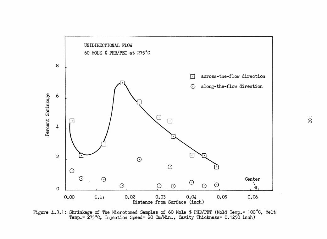
8
2
0 0
0
o.oo
UNIDIRECTIONAL FLOW 60 MOLE % PHB/PET at 275°C
0 0
0 0 0
[] across-the-flow direction
G) along-the-flow direction
0 0 0 Center
\ G.vi 0.02 O.OJ 0.04 0.06
Distance from Surface (inch)
Figure 4.3.1: Shrinkage of The Microtomed Samples of 60 Mole % PHB/PET (Mold Temp.= 100°C, Melt Temp.= 275°C, Injection Speed= 20 Cm/Min., Cavity Thickness= 0.1250 inch)
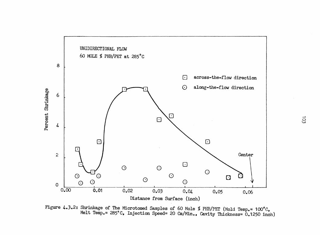
UNIDIRECTIONAL FLOW 60 MOLE % PHB/PET at 285°C
8
c:J across-the-flow direction
() along-the-flow direction 6
4
8
2 Center
G 0 0
0 0 0
0 0 0
0 0
0~00 0.01 0.02 0.03 0.04 0.05 0.06 Distance from Surf ace (inch)
Figure 4.3.2: Shrinkage of The Microtomed Samples of 60 Mole % PHB/PET (Mold Temp.= 100°C, Melt Temp.= 285°C, Injection Speed= 20 Cm/Min., Cavity Thickness= 0.1250 inch)
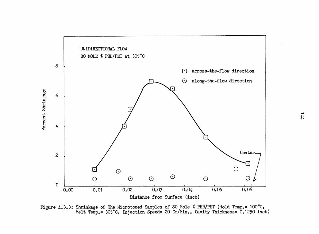
UNIDIRECTIONAL FLOW 80 MOLE % PHB/PET at 305°C
8 (] across-the-flow direction
c::> along-the-flow direction
2
0 0 0 0 G 0 0 0
0 o.oo 0.01 0.02 0.03 0.05 0.06
Distance from Surface (inch)
Figure 4.3.3: Shrinkage of The Microtomed Samples of 80 Mole % PHB/PET (Mold Temp.= 100°C, Melt Temp.= 305°C, Injection Speed= 20 Cm/Min., Cavity Thickness= 0.1250 inch)
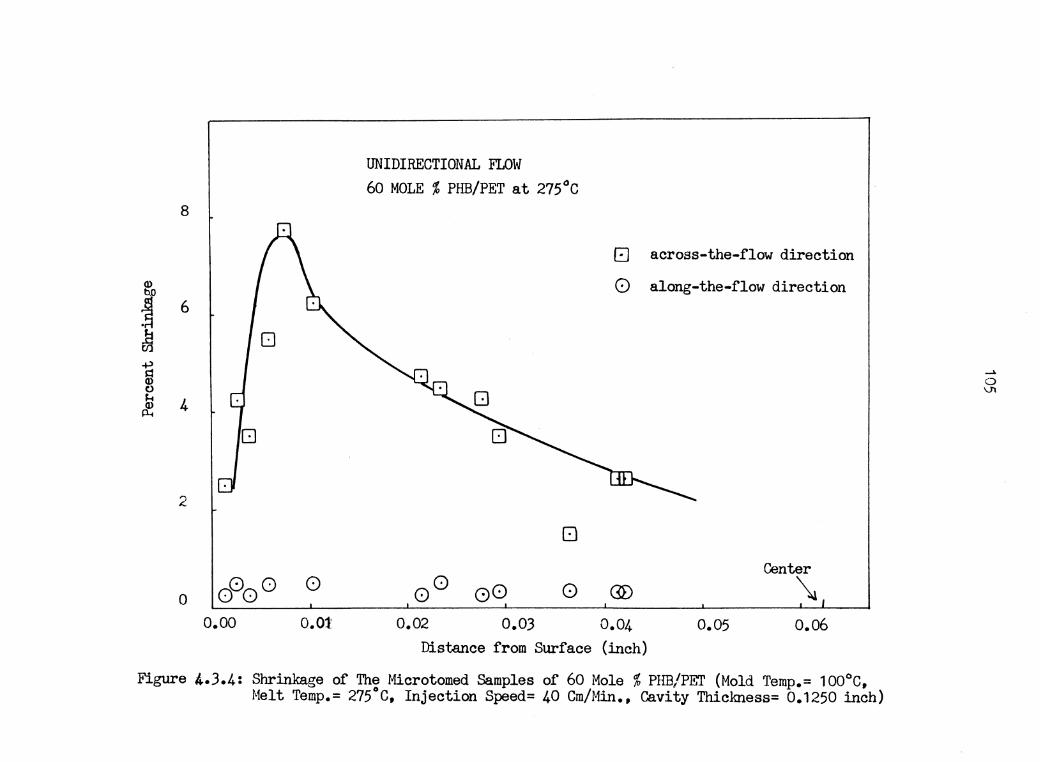
8
0
2
0 0
o.oo o.ot
UNIDIRECTIONAL FLOW 60 MOLE % PHB/PET at 275°C
0 0.02 0.03
GJ across-the-flow direction
0 along-the-flow direction
Center \i
0.04 0.05 0.06 Distance from Surf ace (inch)
Figure 4.3.4: Shrinkage of The Microtomed Samples of 60 Mole % PHB/PET (Mold Temp.= 100°C, Melt Temp.= 275°C, Injection Speed= 40 Cm/Min., Cavity Thickness= 0.1250 inch)
_. 0 Vl

8
6
4
2
0 0 00 0
0 o.oo 0.01 0.02
UNIDIRECTIONAL FLOW 60 MOLE % PHB/PET at 285°C
8
0 0 0 ___a__ ___
0.03
(:J across-the-flow direction
0 along-the-flow direction
0 0
0 Cent\
0.04 0.05 o.06 Distance from Surface (inch)
Figure 4.3.5: Shrinkage of The Microtomed Samples of 60 Mole % PHB/PET (Mold Temp.= 100°C, Melt Temp.= 285°C, Injection Speed= 40 Cm/Min., Cavity Thickness= 0.1250 inch)

8
6
4
2
0 o.oo
UNIDIRECTIONAL FLOW 80 MOLE % PHB/PET at 305QC
0 0 00 0 0 0
0.01 0.02
Q
[]
0 0.03
r::J across-the-flow direction
~ along-the-flow direction
Center 0 0 ~
0.04 0.05 o.06 Distance from Surface (inch)
Figure 4.J.6: Shrinkage of The Microtomed Samples of 80 Mole % PHB/PET (Mold Temp.= 100°C, Melt Temp.= 305°C, Injection Speed= 40 Cm/Min., Cavity Thickness= 0.1250 inch)
..... 0 -.J
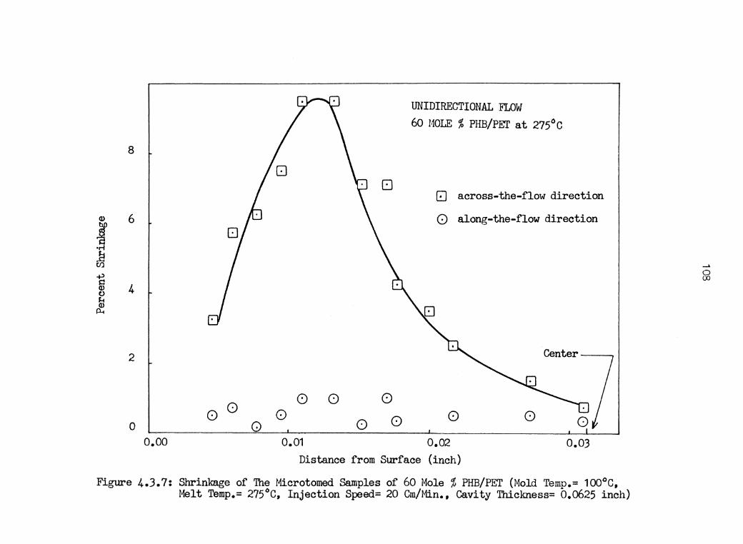
UNIDIRECTIONAL FLOW 60 MOLE % PHB/PET at 275°C
8
G] across-the-flow direction
6 0 along-the-flow direction
4
2 Center--
0 0 0 0 0 0 0 0
0 Q 0 0 o.oo 0.01 0.02 0.03
Distance from Surface (inch)
Figure 4.3.7: Shrinkage of The Microtomed Samples of 60 Mole % PHB/PET (Mold Temp.= 100°C, Melt Temp.= 275°C, Injection Speed= 20 Cm/Min., Cavity Thiclaless= 0.0625 inch)
~
0 (X)
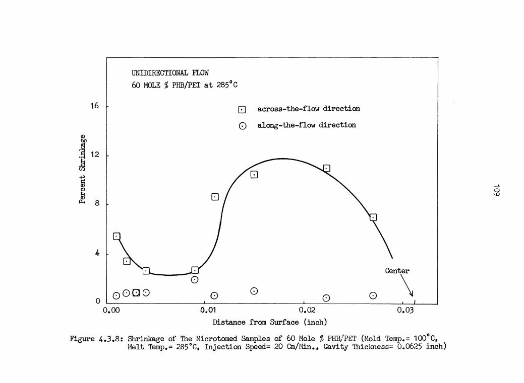
UNIDIRECTIONAL FLOW 60 MOLE % PHB/PET at 285°C
16
4
oOElO 0
o.oo
0 0
0.01
GJ across-the-flow direction
0 along-the-flow direction
0 0
0.02 Distance from Surface (inch)
Center
0 \ 0.03
Figure 4.3.8: Shrinkage of The Microtomed Samples of 60 Mole % PHB/PET (Mold Temp.= 100°C, Melt Temp.= 285°C, Injection Speed= 20 Cm/Min., Cavity Thiclmess= 0.0625 inch)
__. 0 ,0
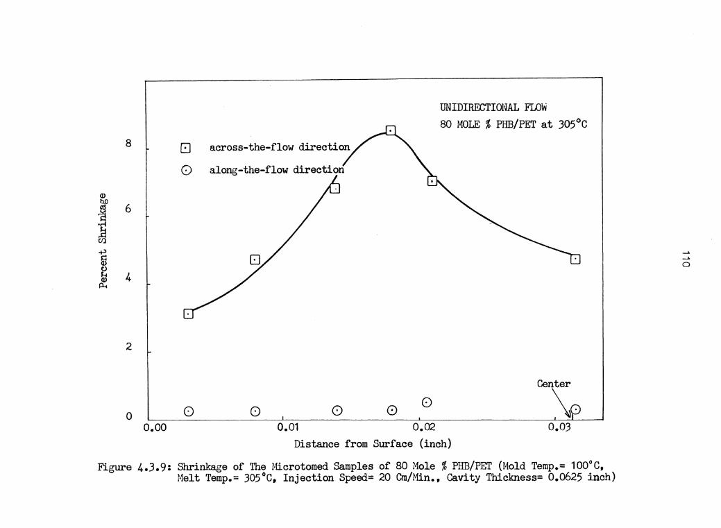
UNIDIRECTIONAL FLOW 80 MOLE % PHB/PET at 305°C
8 8 across-the-flow direction
() along-the-flow direction
2
Center
0 0 0 0 0 \p 0
o.oo 0.01 0.02 0.03 Distance from Surface (inch)
Figure 4.3.9: Shrinkage of The Microtomed Samples of 80 Mole % PHB/PET (Mold Temp.= 100°C, Melt Temp.= 305°C, Injection Speed= 20 Cm/Min., Cavity Thickness= 0.0625 inch)

16
Q) J 12
Jj
1 8
4
0 0 o.oo
UNIDIRECTIONAL FLOW 60 MOLE % PHB/PET at 275°C
0 0 0.01
GJ across-the-flow direction
() along-the-flow direction
Center---.
0 0 0.02 0.03
Distance from Surface (inch)
Figure 4.3.10: Shrinkage of The Microtomed Samples of 60 Mole% PHB/PET (Mold Temp.= 100°C, Melt Temp.= 275.°C, Injection Speed= 40 Cm/Min., Cavity Thickness= 0.0625 inch)
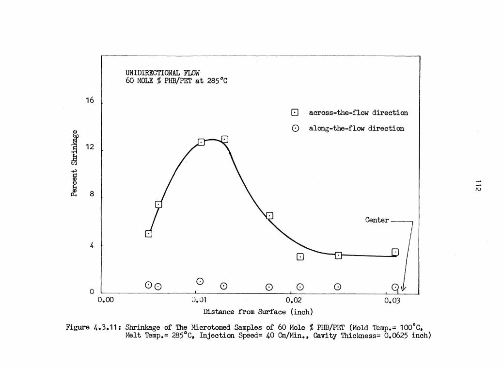
UNIDIRECTIONAL FLOW 60 MOLE % PHB/PET at 285°C
16 c:l across-the-flow direction
0 along-the-flow direction
Center-~
4
0 () 0 0 0 0
o.oo 0.02 0.03 Distance from Surface (inch)
Figure 4.3.11: Shrinkage of The Microtomed Samples of 60 Mole % PHB/PET (Mold Temp.= 100°C, Melt Temp.= 285°C, Injection Speed= 40 Cm/Min., Cavity Thiclaless= 0.0625 inch)

UNIDIRECTIONAL FLOW 80 MOLE % PHB/PET at 305°C
8
Q. across-the-flow direction CD
i 0 along-the-flow direction 6
~ Cl)
fil e CD p... 4
Center
2
0 0 0 0 0 0 0 0 0 0 0 0 o.oo o.o-i 0.02 0.03
Distance from Surface (inch)
Figure 4.3.12: Shrinkage of The Microtomed Samples of 80 Mole % PHB/PET (Mold Temp.= 100°C, Melt Temp.= 305°C, Injection Speed= 40 Cm/Min., Cavity Thicknes~= 0.0625 inch)
_. _. \.JJ

RADIAL FLOW f:IJ MOLE % PHB/PET at 275°C
20
0 8-direction
Q) ~ r-direction
I 15 ~ +> fa (.) J.t 0 if 10
Center 5
0 o.oo 0.01 0.02 0.03 0.04 O.C5 o.06
Distance from Surf ace {inch)
Figure 4.3.13: Shrinkage of The Microtomed Samples of 60 Mole % PUB/PET (Mold Temp.= 165°C, Melt Temp.= 275°C, Injection Speed= 20 Cm/Min., Cavity Thickness= 0.1250 inch)
__.. __.. ~
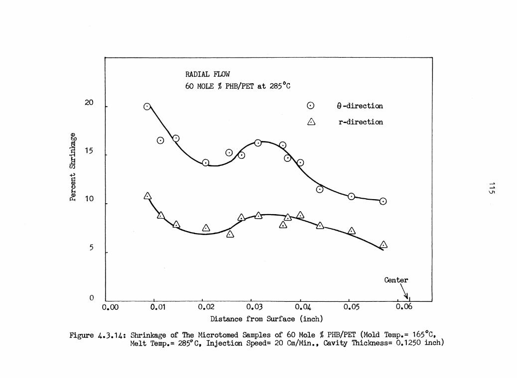
RADIAL FLOW 60 MOLE % PHB/PET at 285°C
20 0 e -direction
~ r-direction Q) jo
15
M +> ai C)
~ 10
5
Center
0 \ o.oo 0.01 0.02 O.OJ 0.04 o.os 0.06
Distance from Surface (inch)
Figure 4.J.14: Shrinkage of The Microtomed Samples of 60 Mole % PHB/PET (Mold Temp.= 165°C, Melt Temp.= 285°C, Injection Speed= 20 Cm/Min., Cavity Thickness= 0.1250 inch)
__. __. \J'l
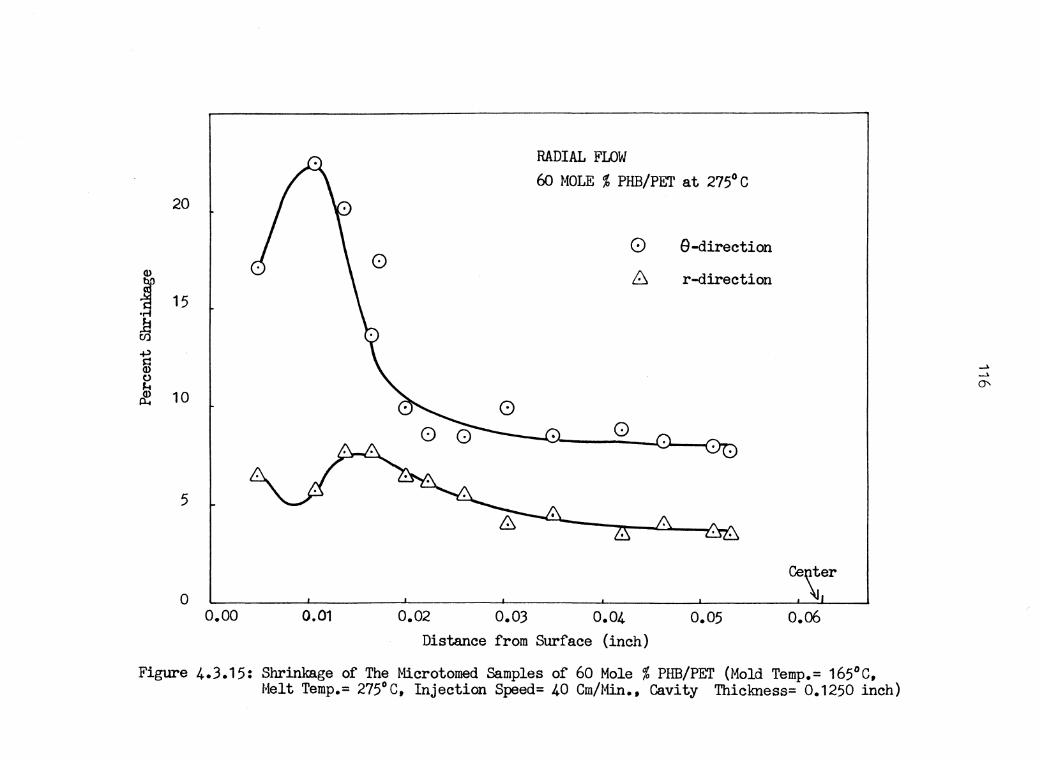
RADIAL FLOW 60 MOLE % PHB/PET at 275°C
20
0 9-direction
r-direction
5
0 o.oo 0.01 0.02 O.OJ 0.04 0.05 o.06
Distance from Surface (inch)
Figure 4.J.15: Shrinkage of The Microtomed Samples of 60 Mole % PHB/PET (Mold Temp.= 165°C, Melt Temp.= 275°C, Injection Speed= 40 Cm/Min., Cavity Thickness= 0.1250 inch)
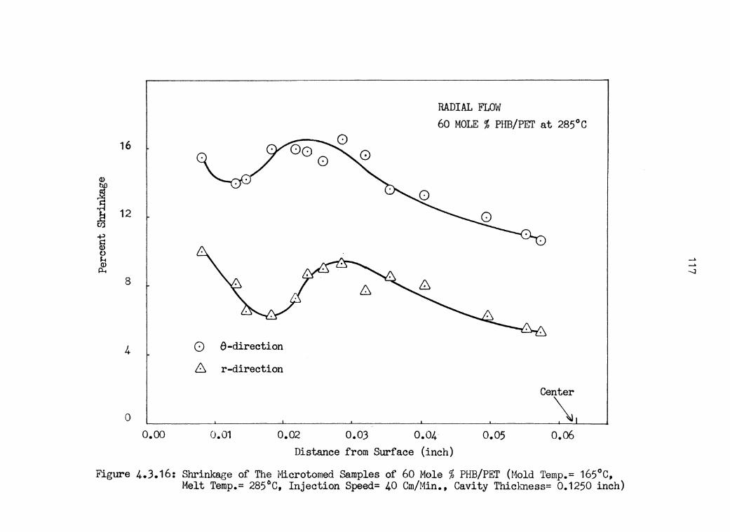
RADIAL FLOW 60 MOLE % PHB/PET at 285°C
16
8
4 () e-direction
r-direction
Center
0 \ o.oo 0.01 0.02 0.03 0.05 o.06
Distance from Surface (inch)
Figure 4.3.16: Shrinkage of The Microtomed Samples of 60 Mole% PHB/PET (Mold Temp.= 165°C, Melt Temp.= 285°C, Injection Speed= 40 Cm/Min., Cavity Thickness= 0.1250 inch)

RADIAL FLOW 60 MOLE % PHB/PET at 275°C
20 0 9-direction
~ r-direction
15
10
5
6
0 Cente~
o.oo 0.01 0.02 0.03 Distance from Surface (inch)
Figure 4.3.17: Shrinkage of The Microtomed Samples of 60 Mole% PHB/PET (Mold Temp.= 165°C, Melt Temp.= 275°C, Injection Speed= 20 Cm/Min., Cavity Thickness= O.o625 inch)
-' -' 00
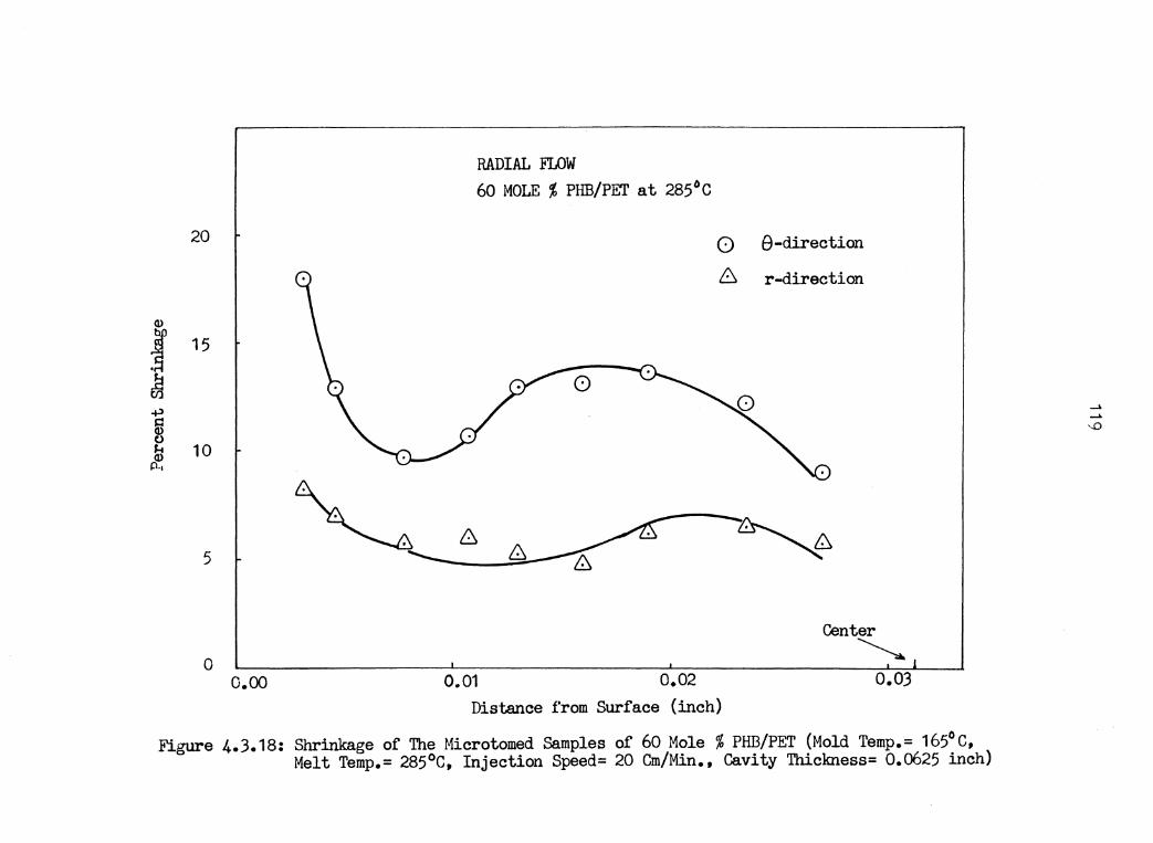
RADIAL FLOW 60 MOLE % PHB/PET at 285°C
20 0 6-direction
6 r-direction
(1)
I 15
~ 0 +> 53 (.) J..I 10 Cl)
p.,
5
Center
0 ~ o.oo 0.01 0.02 0.03
Distance from Surf ace (inch)
Figure 4.3.18: Shrinkage of The Microtomed Samples of 60 Mole % PHB/PET (Mold Temp.= 165°C, Melt Temp.= 285°C, Injection Speed= 20 Cm/Min., Cavity Thickness= 0.0625 inch)
_. ...... -..o

20
Q)
J 15
~ ~ Q) 0 J... 10 ~
5
0 o.oo
RADIAL FLOW 60 MOLE % PHB/PET at 2?5°C
0 6-direction
~ r-direction
0.01 0.02 Distance from Surface (inch)
G 0 0
Center
~ 0.03
Figure 4.3.19: Shrinkage of The Microtomed Samples of 60 Mole % PHB/PET (Mold Temp.= 165°C, Melt Temp.= 2?5°C, Injection Speed= 40 Cm/Min., Cavity Thiclmess= 0.0625 inch)
__. /\.) 0
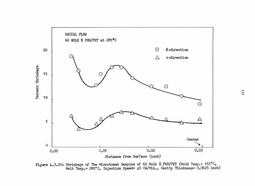
20
Q)
J 15
~ +:> ~ Q) () ~ Q)
p.. 10
0 o.oo
RADIAL FLOW 60 MOLE % PHB/PET at 285°C
0.01 0.02
0 8-direction
6 r-direction
0
Center ~
0.03 Distance from Sl.ll"f ace (inch)
Figure 4.3.20: Shrinkage of The Microtomed Samples of 60 Mole % PHB/PET (Mold Temp.= 165°C, Melt Temp.= 285°C, Injection Speed= 40 Cm/Min., Cavity Thiclmess= 0.0625 inch)
..... /\) .....

UNIDIRECTIONAL FLOW 60 MOLE % PHB/PET at 275 C
8
0
6 0 -Q) [] hf) m 0 ~
•rl l:! D U)
0 -+> ~ 4 (.) 0 H Q)
P-.
8 0 B
2 ..
0 o.oo o.01 0.02
0 oD
0 0
0
0.03 0.04
0
0
r
0 00 0
Cienter . I
0.05 o.06 Figure 4.3.21: Comparison of the Across the Flow Shrinkage of the Microtomed samples of 60 Mole %
PHB/PET in two separate runs (Injection Speed= 20 Cm/Min, Cav. Thick.= 0.125 inch)

Chapter V
DISCUSSION
5.1 VISCOSITY MEASUREMENT
The first objective of this work was to determine whether
a boundary layer effect existed for liquid crystalline po-
lymers. The approach used to determine this effect was to
measure viscosity of these polymers as a function of shear
rate at different temperatures using capillaries with diffe-
rent diameters. As observed in chapter 4, the shear rate
range was limited to fairly high shear rates (from 40 to
5000 sec1 ) in the capillary rheometer. As a result, the vis-
cosity shear rate curves show the high-shear behavior of
these liquid crystalline fluids. The procedure to obtain
the viscosity-shear rate curves was outlined in chapter 4.
Basically, the corrected wall shear stresses were obtained
from the pressure data and corrected for the entrance pres-
sure loss by constructing the Bagley plot. The power law
melt flow indices were calculated from the slope of log of
wall shear stress versus log of apparent shear rate. This
value was then used to calculate the corrected wall shear
rate, and from this the viscosity-shear rate curves were ob-
tained.
123

124
The viscosity-shear rate curves of these polymers are
shown in figures 4.1.13 to 4.1.19. When compared at the same
melt temperature, PET/60 mole % PHB shows a much lower vis-
cosi ty than that of PET homopolymer. Typically, at 275° C -·1 and shear rate of 1000 sec ,viscosity of PET homopolymer is
61. 73 Pascal. Sec. whereas that of PET/60%PHB is 2. 8 Pas-
cal.Sec .. This can be explained in terms of an ordering ef-
feet. In general, the 60%PHB/PET molecules are more rigid
than PET molecules. During flow they are readily oriented
along the lines of the flow by the shear field. This re-
sults in lower viscosity than in the isotropic state.
In figures 4.1.13 to 4.1.15, viscosity of PET/60%PHB at
275cC shows an overlap with those at 260 and 285°C. This is
due to a change in viscosity when measured using capillaries
with different diameters. This phenomena will be discussed
in more detail in the next section (boundary layer effect).
Many difficulties were encountered in obtaining repeata-
ble values of viscosity, i.e. the position of plunger in the
Instron barrel, the thermal history of the melt before ex-
periment. A special experimental technique was developed
and reported in chapter 3 in order to obtain repeatable re-
sults. For the purpose of confirming this experimental tech-
nique, figures 5.1.1 to 5.1.7 show the viscosity-shear rate
curves between the data of this work, the data obtained from
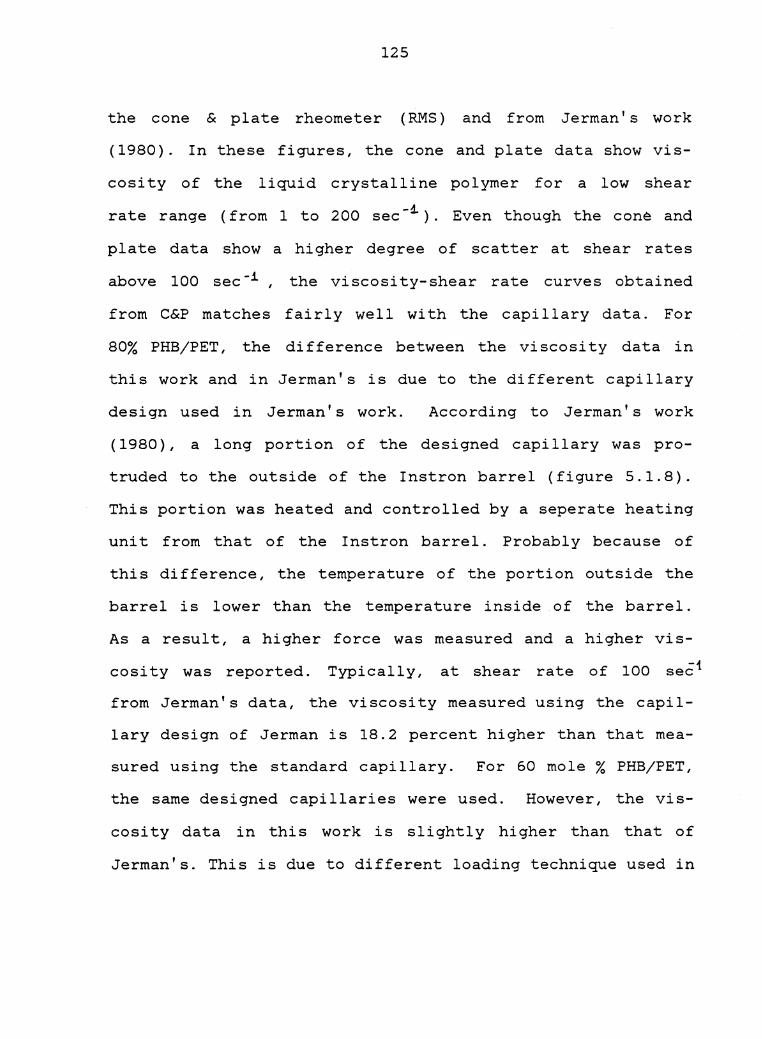
125
the cone & plate rheometer (RMS) and from Jerman' s work
(1980). In these figures, the cone and plate data show vis-
cosity of the liquid crystalline polymer for a low shear
rate range (from 1 to 200 sec-~). Even though the cone and
plate data show a higher degree of scatter at shear rates
above 100 sec-i , the viscosity-shear rate curves obtained
from C&P matches fairly well with the capillary data. For
80% PHB/PET, the difference between the viscosity data in
this work and in Jerman's is due to the different capillary
design used in Jerman' s work. According to Jerman' s work
( 1980), a long portion of the designed capillary was pro-
truded to the outside of the Instron barrel (figure 5.1.8).
This portion was heated and controlled by a seperate heating
unit from that of the Instron barrel. Probably because of
this difference, the temperature of the portion outside the
barrel is lower than the temperature inside of the barrel.
As a result, a higher force was measured and a higher vis-
cosity was reported. Typically I at shear rate of 100 sec1
from Jerman's data, the viscosity measured using the capil-
lary design of Jerman is 18.2 percent higher than that mea-
sured using the standard capillary. For 60 mole % PHB/PET,
the same designed capillaries were used. However, the vis-
cosity data in this work is slightly higher than that of
Jerman's. This is due to different loading technique used in

126
Jerman's work. In this work, the polymer pellets are loaded
into the Instron barrel in a standard experimental procedure
as described in chapter 3. However, according Jerman, he
found that the 60 mole % PHB/PET pellets melted too rapidly
and adhered to the side of the resevoir, causing a bridging
effect across the month of the barrel. As a result, he used
a different loading procedure to perform his experiment. In
his work, the 60 mole % PHB/PET polymer pellets were com-
pression molded into a polymer rod and subsequently, the rod
was loaded into the Instron barrel. This procedure would
cause the polymer to decrease in molecular weight. The ef-
fect of the higher viscosity results from the use of the
protruding capillary of Jerman is probably less than the ef-
fect of the lower viscosity results from the loss in molecu-
lar weight. As a result, for PET/60%PHB, a lower viscosity
was measured in Jerman' s work than that reported in this
work.
As shown in figures 5.1.6 and 5.1.7, values for melt vis-
cosities of PET homopolymer are less than those measured by
RMS and Jerman. This could possibly due to degradation or
hydrolysis of the sample. Extrudate was collected for PET
homopolymer and run again to check for changes in pressure,
as a check for possible polymer degradation. For PET homo-
polymer at 275 and 285°c, with the resident time of the melt

127
in the Instron barrel of one minute, the pressure reading
was the same as that of the original run. This indicates
that PET samples used in this experiment had been degraded.
The process of degradation is probably due to hydrolysis of
the polymer (Van Der Wielen, 1975). Since degradation is the
result of a chemical reaction, it is evident that the extent
to which the material degrades will not only depend upon the
amount of moisture present but will also depend on the time
over which the reaction is allowed to proceed, i.e. the re-
sident ,time of the melt. To show this effect, a sample of
PET was run at 275 and 285°C, with the resident time of five
minutes, the pressure reading was lower on this run by 48.7
% at 275°C and 59.5 % at 285°C when compared with the ori-
ginal run. From these experiments, it is obvious that the
rheological property of PET is a strong function of both
moisture content and the resident time of the melt. Care
must be taken to eliminate these interference in future ex-
periments with this material.
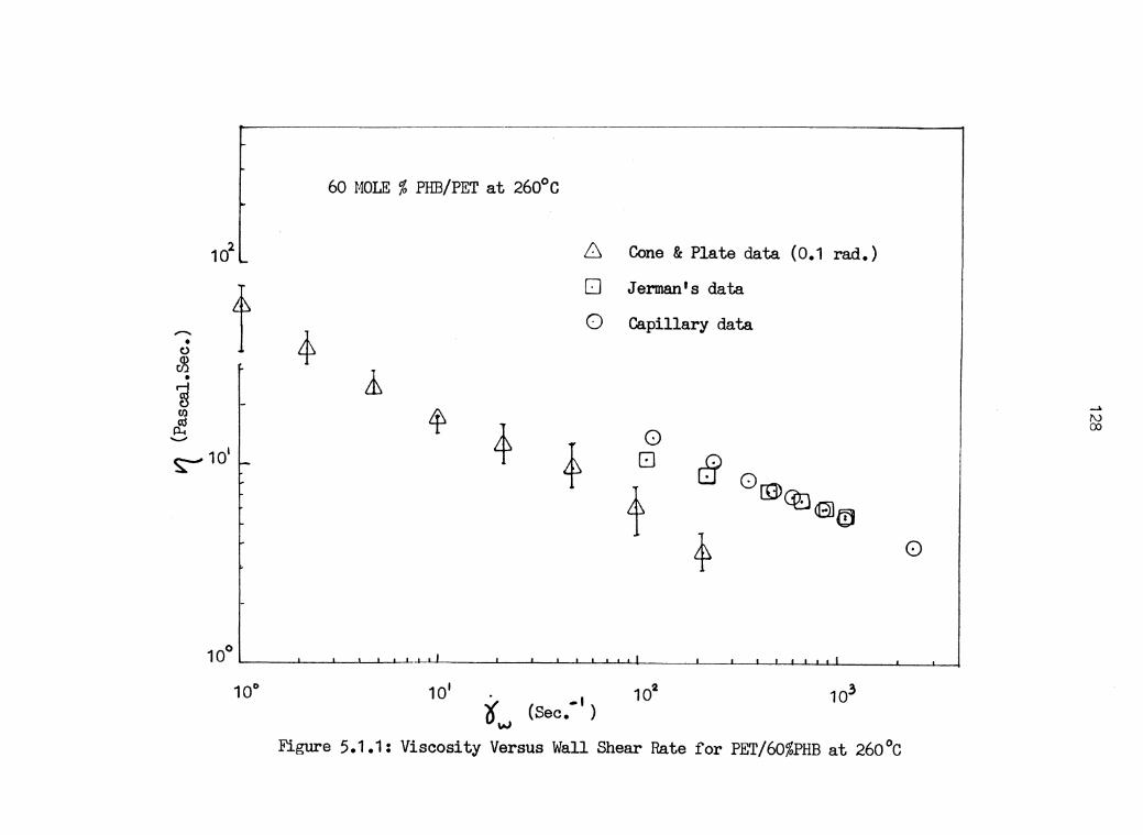
t I s:-10 ~
10°
60 MOLE % PHB/PET at 260°C
101
6 Cone & Plate data (0.1 rad.)
D Jerman's data
() Capillary data
t _, (Sec. ) w
0 8
+ 8 0
~
[3)~ (8)Cl
Figure 5.1.1: Viscosity Versus Wall Shear Rate for PET/60%PHB at 260°c
_. I\) 00
0
........... • (.)
J3 • ~ (/)
~ ......... 1o'
~ f-
60 MOLE % PHB/PET at 275°C
e 8one & Plate data (0.1 rad.)
0 Jerman's data
0 Capillary data
a 10°.__~---L-~-'-----'----'---'-~'-L-L·~~-'-~"'--~'-'--'-'---1-1..~·~~_i___J~L__j_J_l_L_L_J_i_l~~i·~-L---l
10° i"w (Sec.- I)
Figure 5.1.2: Viscosity Versus Wall Shear Rate for PET/60%PHB at 275°C

60 MOLE % PHB/PET at 285°C
102 i-.. 6 Cone & Plate data (0.04 rad.)
0 Jerman's data - 4 ~ 0 Capillary data • 4 () <I> t Cl)
t • ~ t t/l t __. ~ w
0 .._,. I 4 ~
10 ... 4o 0 £x:J
[] Ooo [] 0
0 [] 0 Dc:::i 0
10° I I I I I I
10° 10 1 t (Sec.- 1 ) 102 103
w Figure 5.1.3: Viscosity Versus Wall Shear Rate for PET/60%PHB at 285°C

80 MOLE % PHB/PET at 305°C
~ Cone & Plate data (0.1 rad.) 102 - 0 Jerman's data
~ ~ 0 Capillary data - Cl •
~ () Q)
Cl) ~ • 8 c::i (/) ...
~ 0 8! ...... "" ........ 0 ......
I c::i c:J 0 s:--' 10 f- (:J (:J
@00 8 r::J
['.] [:J 0 ·o
0 Oo
10°1--~_._·~~·_._-'-~'-'-'--Jl'-----~~·'------'-~·L_J._·~·L-L.JL.LL.l~~~'~~·__,__..___._11~•~·__._.__'~~-'--'-4-'-i..'-'----'-'..L-J
10° 101 Yw (Sec. -I)
Figure 5.1.4: Viscosity Versus Wall Shear Rate for PET/80%PHB at 305°C

80 MOLE % PHB/PET at 315°C
6 Cone & Plate data (0.1 rad.)
10'f 0 Jerman's data
1 0 Capillary data ........
• & () Q) ...
Cf.)
~ • ~ & rJl
~ ... &
_. 'v.J ......... I\)
~101 ¢ [] -
b 0 ... 4 4 0 ... f 00
0 8 Oo 0 Oo
0 10° I I I I I I I I I I I I I I I I I I I I I I I I I I I I
10° 10 1 ow (Sec.- 1 ) 10 2 10 3
Figure 5.1.5: Viscosity Versus Wall Shear Rate for PET/80%PHB at 315°C

,....... •
()
~ • 'cl () t/l
&! .._..
s;:..J
~ 10
2.. 10
10 I
EJ
0 .IO
PEI'/HOMOPOLYMER at 275°C
6 6 ~ 6 6 6 66 EJ [J EJ [J 8 EJ ....... w r:J w
0 0 0 00 00 0 0 0 Cone & Plate data (0.1 Rad.)
& Jerman's data
0 Capillary data
LI
10 1 10a 103
0-\J _, (Sec. )
Figure 5.1.6~ Viscosity Versus Wall Shear Rate for PET/Hornopolymer at 275°C
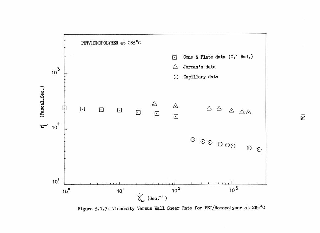
10'
10° 10' -/ {Sec.- I ) Ow
0 0 . 8 0 00 8 8
Figure 5.1.7: Viscosity Versus Wall Shear Rate for PET/Homopolymer at 2g5cic

135
RETAINING RING
CAPILLARY
/ / .__..._
(A) SIANOARO DESiGN (3) REVISED DESIGN
Figure 5.1.8: Schematic Diagram of Capillary used in this Work (A) and That used by Jerman (B), (Jerman,1980)
136
5.2 BOUNDARY LAYER EFFECTS ON VISCOSITY
In. connection with the first section of this chapter,
this section will discuss the possibility of a boundary lay-
er effect in more detail. The viscosity of PET/60%PHB and
PET/80%PHB was measured using three capillary sets with
different diameters _ 6. 858 ( 10-4- ) , 1. 27 ( 10-3 ), and 1. 778 ( 163
) meter (corresponding to 0.027, 0.050, and 0.070 inches).
For each capillary diameter, three capillaries with diffe-
rent L/D ratio were used to obtain the entrance pressure
loss by constructing the Bagley plot. Viscosity data using
capillaries with diameters indicated above are plotted
against wall shear rate. For 60 mole % PHB/ PET, the viscos-
ity-shear rate curves are shown in figures 5.2.1 to 5.2.3 at
temperatures of 260, 275 and 285°c. Similarly, for 80 mole %
PHB/PET, in figures 5.2.4 and 5.2.5, these curves are shown
at two temperatures of 305 and 315 ° C. From these curves,
only the viscosity data of PET/60%PHB measured at 275 ° C
shows an increase with increasing capillary diameter. As a
result, this causes an overlap in viscosity data when plot-
ting viscosity-shear rate curves for different temperatures
on the same graph (see figures 4. 1. 13 to 4. 1. 15) . This re-
sult leads to two immediate questions: (1) How does this
possible phenomena occur ? (2) Why does it only occur at
275°c and not at 260°c nor at 285°c ? These questions will
be discussed seperately in the subsequent paragraphs.

137
Before trying to answer these questions, one needs to
investigate the role of entrance pressure loss in this pos-
sible phenomena. Entrance pressure loss can be thought of
as the pressure associated with the energy needed to over-
come a polymer's elastic resistance to converging extension-
al flow. According to the theory of capillary rheometry,
this entrance pressure is independent of the capillary geo-
metry, i.e. the L/D ratio. Figures 5.2.6 to 5.2.10 show
plots of 0 ~n vs apparent shear rate for the three capil-
lary sizes used. In general, the entrance pressure data
show good agreement with the hypothesis of capillary flow -f stated above in the range of shear rates up to 200 sec
Above this range, deviation from the theory occur. To minim-
ize the effect of entrance pressure loss, a long capillary
was used so that the pressure drop over the entrance region
was negligible compared with the pressure drop over the en-
tire length of the capillary. Figure 5.2.11 shows the vis-
cosity of 60 mole % PHB/PET at 275°c using the longest ca-
pillaries for each capillary diameter. Again, the dependence
of viscosity on capillary diameter is observed.
The answer to the first question may be related to the
molecular orientation at the boundary which can be caused by
physical defects or textures on the surf ace or any chemical
treatment of that surface (Berreman, 1973). Throughout the
138
experimental procedure, no chemical treatment was applied
and it is assumed that none was applied to the inside of the
capillaries during their manufacture. Using a scanning elec-
tron microscope, Jerman ( 1980) showed that there exists a
strong pattern of grooves running longitudinally in the flow
channel. This pattern is probably the result of the drawing
process commonly used in manufacture of tubing. The texture
in the tubing is clearly one of long parallel grooves in the
flow direction which would cause an orientation parallel to
the grooves and consequently parallel to the flow (Berreman,
1973; Fisher and Fredrickson, 1969; Jerman, 1980). Probably,
the increase in viscosity with increasing in capillary diam-
eter is due to this texture of the tube wall (capillary
wall). This result is in agreement with the work by Fisher
and Fredrickson (1969) who found similar results for the ca-
pillary flow of low molecular weight liquid crystalline po-
lymer (p-azoxyanisole) with the capillary specially treated
with sulfuric acid-dichromate.
This boundary layer effect can be summarized as follows.
At the boundary, there exists a layer of molecules with
different orientation from those in the core. Because of the
special molecular orientation, this layer has its own vis-
cosity which is less than that of the core fluid. The thick-
ness of this layer is presumably a function of both tempera-

139
ture and shear rate. As the cross section of the capillary
decreases (capillary diameter decreases), the cross section
area taken up by this boundary layer increases. Consequent-
ly the bulk viscosity of the fluid inside the capillary is
affected by this boundary layer and thus decreases (with de-
creasing capillary diameter).
The fact that the boundary layer effect only occurs at
275°c may be explained from the molecular kinetic energy as-
sociated with the solid-nematic and nematic-isotropic tran-
sition. From Boltzman distribution, ifA E is the difference
in free energy per molecule between solid state and nematic
mesophase, then the number of molecules having this energy
is proportional to exp (-~ E/kT) (Pincus and de Gennes,
1977). At low temperature, not many molecules possess this
energy to undergo solid-nematic transition; a semicrystal-
line results in the melt. As the temperature increases, more
molecules obtain this energy, thus the solid-nematic transi-
tion occurs. Consequently, at this temperature, the boundary
layer effect on viscosity is observed. Further increase in
temperature would make these molecules to gain more energy,
sufficient to undergo Brownian motion. As a result, nematic-
isotropic transition occurs and therefore the boundary layer
effect on viscosity is not observed.
140
Molecules in isotropic state are freely rotating. In con-
trast, molecules in nematic mesophase are packed such that
they have freedom of rotion about one axis only (R. Wil-
liams, 1963). The heat for solid-nematic-isotropic transi-
tions thus involved energy for both molecular seperation and
internal rotation (Barrall et al., 1964). To further inves-
tigate this explanation, future works should study the heat
required for these transitions using differential scanning
calorimetry. Also, since the molecular rotation of molecules
in isotropic state is different from that of nematic meso-
ph~se, NMR spectra for melt in nematic mesophase is expected
to be different from that in isotropic state. Further work
should include NMR studies for these states.

1 () 0
10 1
60 MOLE % PHB/PET at 260°C
t"°' (Sec.- I )
Capillary Diameter, i!!£!1
0 0 6
0.02?
0.05
o.o?
104-
Figure 5.2.1: Comparison of Viscosity for PET/60%PHB Measured at 260°C Using Capillaries with Different Diameters
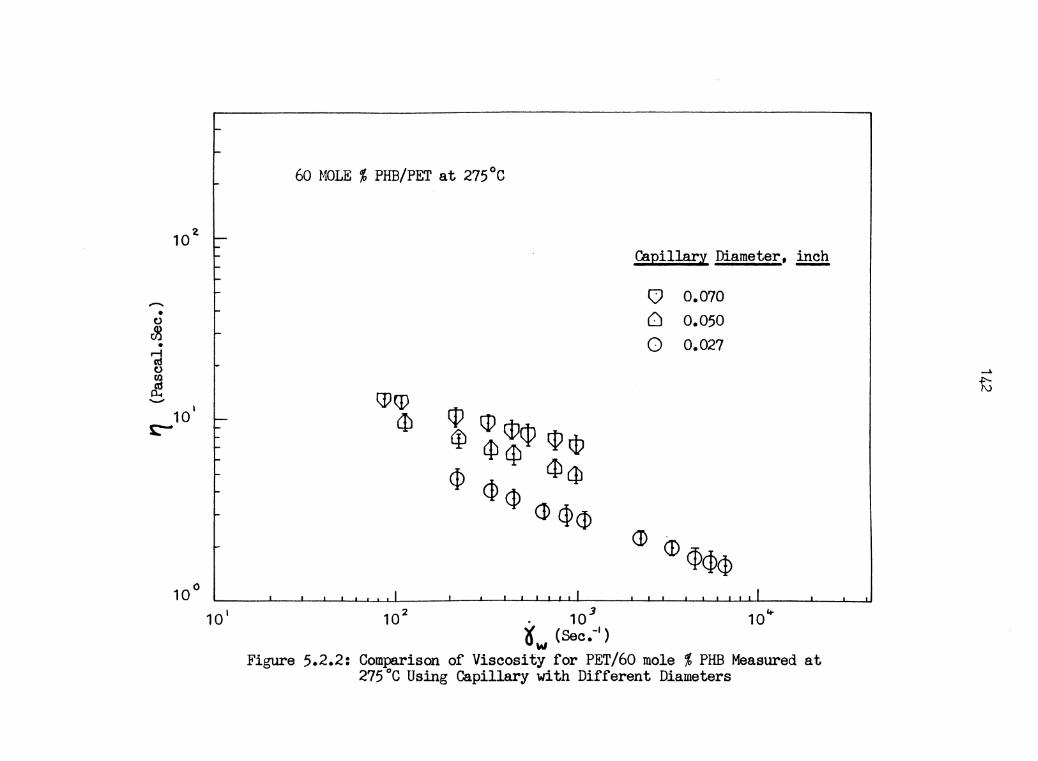
10 2
......... •
()
t93 • r-1 m () Cl)
&! ......... 10 1
c-
60 MOLE % PHB/PET at 275°C
Capillary Diameter, ~
CJ 0.070 Q o.oso 0 0.027
\Pq) (}) cp cp cP
i{l iii qi q:i ~ qi <P c:D $
<P ell ~ <P <!> <1)
© (f)¢cp
10 1 10 2 • 10 3 10* ~ (Sec.-')
w Figure 5.2.2: Comparison of Viscosity for PET/60 mole % PHB Measured at
2?5°C Using Capillary with Different Diameters
_. .p-... I\}

60 MOLE % PHB/PET at 285°C
Oapillary Diameter, i!!£h.
Q 0.07
a 0.05
0 0.027
~w (Sec.- 1 )
Figure 5.2.3: Comparison of Viscosity for PET/60%PHB Measured at 285°C Using Capillaries with Different Diameters

102.
-• ()
J3 • ~ [I}
~ ....... ~ 101
80 MOLE % PHB /PET at 305°C
Capillary Diameter, ~
0 0.01
8 0.05
0 0.027
0 ~62@
4)~ ~o~lR 8 00
~~ (Sec.- I )
Figure 5.2.4: Comparison of Viscosity for PET/80%PHB Measured at 305°c Using Capillaries with Different Diameters
_. ~ ~
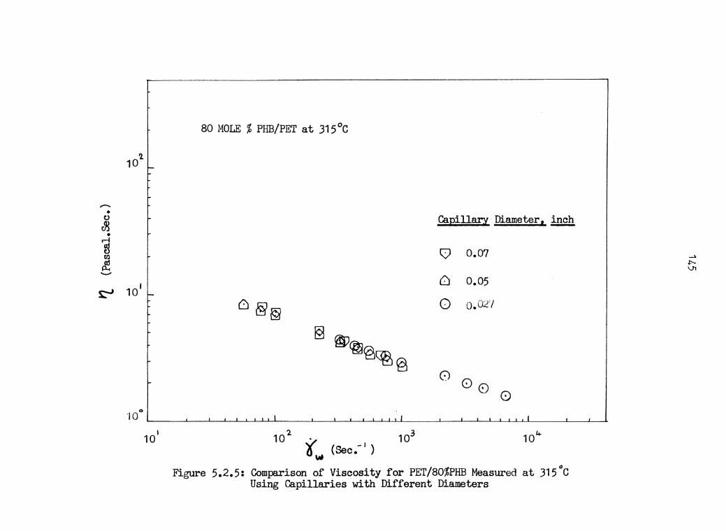
-• t}
~ • .-I ~ {/)
~ .._..
£'""' 101
0 ·10
80 MOLE % PHB/PET at 315 °C
'( (Sec.-' ) w
Capillary Diameter, ~
CJ 0.07
a 0.05
0 0.02'/
8 0 ·0 0
101+
Figure 5.2.5: Comparison of Viscosity for PET/80%PHB Measured at 315°C Using Capillaries with Different Diameters
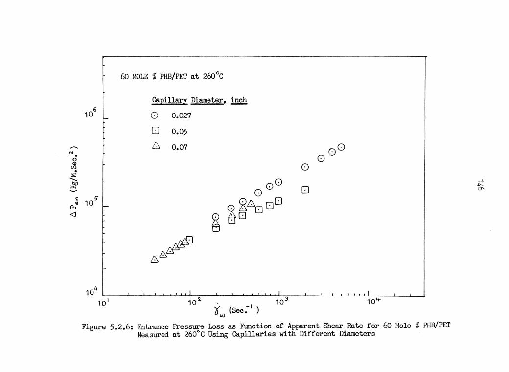
-... • ()
c?3 • ::E: ......... ~ -~ ~
P-t <J
10 5
104
60 MOLE % PHB/PET at 260°C
Capillary Diameter, !!!5ll:! 0 0.027
D 0.05
6 0.07 0
0
0 0
"--;-~-J-~~--'---'--4-'-l-L.L-;;-~_L_~L--.L__l-L--'----L--L-L---.--~_J___Jl__L__J"---.L..LL-1-L.-,-~..L_--1--1
10 1 10~ 103 10~ t. (Sec: I ) w Figure 5.2.6: Entrance Pressure Loss as Function of Apparent Shear Rate for 60 Mole % PHB/PET
Measured at 260°C Using Capillaries with Different Diameters ·

-('I • (.)
JJ • ~ ......... ~ ........ ~
~I/I
<J 105
60 MOLE % PHB/PET at 275°C
Capillary Diameter, ~
0 0.027
0 0.05
u 0.01
0
0
0 (i)
0
1 -.'+-i,) ,___ _ __,__.....___.__.__.___.__,__._._ __ _.___,.__..__.'---L--'---L....L..L. __ _.____J_L_J-.L..LJ._.L.l----L---1---1
101 iw (Sec_- I)
Figure 5.2.7: Entrance Pressure Loss as F\Jnction of Apparent Shear Rate for 60 Mole % PHB/PET Measured at 275°C Using Capillaries with Different Diameters

-°' • (.)
c?J • :::E: ......... ~ ..._..
t: fl.. QI
<l 105
60 MOLE % PHB/PET at 285°C
Capillary Diameter, i!!£h
0 0.027
0 0.05
6 0.07
0 0
0 0 0
0
10* .__~--i.~~~~~~~~~~~~.._..~.__._._~~~~~-'-'--'-_.__.._._._~~__.___.~
10 1 . I '6 w (Sec.- )
Figure 5.2.8: Entrance Pressure Loss as Function of Apparent Shear Rate for 60 Mole % PHB/PET Measured at 285°C Using Capillaries with Different Diameters
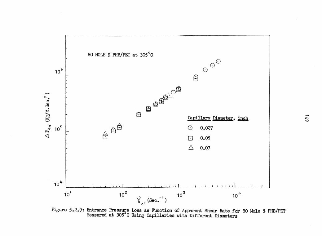
-"' • t) Q)
Cl) • ~ ........ ~ ......... ~ 1\1 p..
<l
80 MOLE % PHB/PET at 305°C
105
10 1
'{ (Sec.-' ) w
8 0 0
Capillary Diameter, 1!!£h 0 0.027
0 0.05
6 o.o?
10 u.
Figure 5.2.9: Entrance Pressure Loss as Function of Apparent Shear Rate for 80 Mole % PHB/PET Measured at 305°C Using Capillaries with Different Diameters
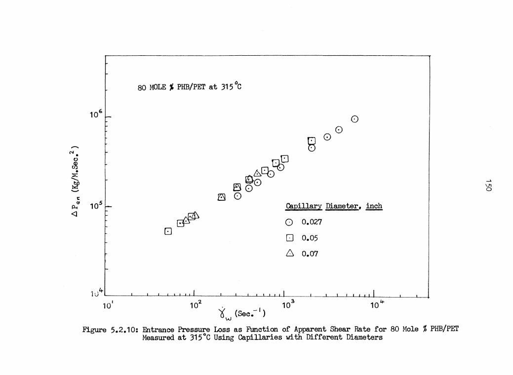
-('I •
()
~ • ~
.......... ~ ........ ~ (:I
P-4 <l
80 MOLE% PHB/PET at 315°C
105
0 0 8 0
Capillary Diameter, .!!!£h 0 0.027
0 0.05
6 0.07
10*'--~--'---~---'---'-_L_Jc_L_LLJ.~~_l_~L__J_.L_L~--LJ_~~_j___JL__l_L_j__J_J__j_J_~~J___J~ 102 10 1
't (Sec.- 1) w Figure 5.2.10: Entrance Pressure Loss as Function of Apparent Shear Rate for 80 Mole% PHB/PET
Measured at 315°C Using Capillaries with Different Diameters
~
V1 0
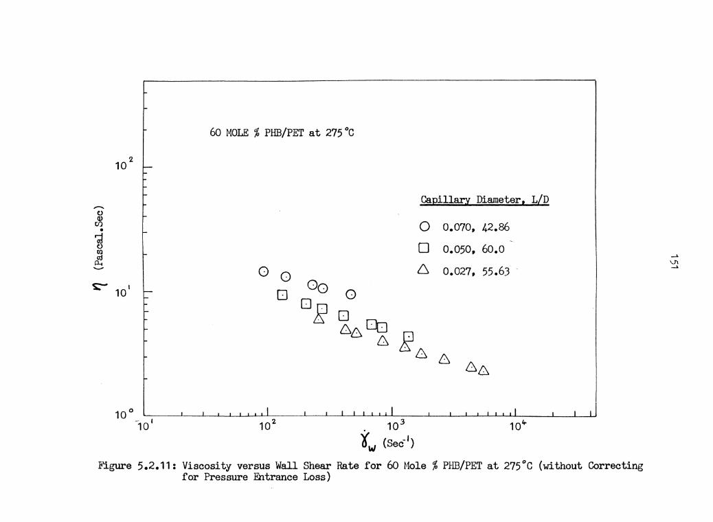
~
() Q)
Cl) •
'cl () (J)
~ .........
s:- 10 1
60 MOLE% PHB/PET at 275°C
0 0 Oo D OR
103
iw (Sec- 1)
Capillary Diameter,
0 0.070, 42.86
0 0.050, 60.0
6 0.027, 55.63
10~
L/D
Figure 5.2.11: Viscosity versus Wall Shear Rate for 60 Mole% Prill/PET at 275°C (without Correcting for Pressure .Entrance Loss)
~
VI ~
152
5.3 MOLD FILLING CHARACTERISTICS
The second objective of this work was to investigate the
mold filling behavior of liquid crystalline polymers. The
procedure used to observe the flow front behavior was dis-
cussed in chapter 3 and 4. The behavior of the flow front of
PET, PET/ 60 mole % PHB, and PET / 80 mole % PHB melts for
flow into a rectangular mold is observed as reviewed in sec-
tion 2.3. The mold filling may be divided into three stages
(figure 2.3.2). First, at the region near the gate, the melt
enters the mold in a radial manner. Secondly, as the melt
reaches the corners, the flow front starts changing its
shape from circular to a nearly flat flow front. Third, the
melt continues to move forward, until the mold is completely
filled by an advancing front mechanism.
Pigmented polymer was introduced into the barrel in an
order so that the blue would enter the mold first, then the
red, green, orange and finally violet. From the video tape
recorded during the flow, it is observed that the order of
the colors which enter the mold is reversed. The blue color
enters the mold first but ceases to flow near the entrance
of the mold. The red color enters next and also ceases to
flow just next to the blue color and away from the gate. Si-
milarly, the green and orange colors move in the same fash-
ion as the red color. The violet color is located at the
153
other end of the mold. Figure 5. 3 .1 shows the shapes of
these colors in a molded plaque. Near the entrance of the
mold, the blue color forms a circular shape corresponding to
the radial flow in the first stage discussed above. The cir-
cular shape of these colors changes to a flat profile as the
polymer melt flows down the cavity away from the gate re-
gion. This would correspond to the second and third stages
of the filling.
The reversion of the order of GOlors entering the mold
can be further investigated by observing their velocities as
a function of time. For the injection of PET homopolymer
into a regtangular mold (figure 5.3.2), the blue and red co-
lors enter first and cease to flow after a certain amount of
tme flowing in the mold. The green and orange colors enter
the mold successively with a velocity higher than those of
the blue and red colors. The violet color enters the mold
last with a higher velocity than the rest of the colors.
From the foregoing discussion, it is evident that at one
time a fluid particle had been flowing in the core and must
reach the flow front. At this point, the fluid particle is
split and flows up to the cold wall of the mold. It is then
frozen and ceases to flow due to this cold wall. Similar ob-
servations have been reported in the work of Schmidt (1976).

154
The mechanism of the splitting pattern at the flow front
is discussed by Tadmore (1974) and reviewed in chapter 2. To
actually investigate this mechanism for the liquid crystal-
line polymer, one must be able to see the movement of these
colors in the core. Figure 5.3.3 and 5.3.4 show photographs
of "short shots" sectioned along the flow for PET/ 60 mole %
PHB and PET/ 80 mole % PHB, respectively. For PET/ 60 mole
% PHB (figure 5. 3. 3), the blue and red colors lay on the
wall. The green color is splitting at the front. What is un-
usual is that the orange and violet colors are splitting
even when they are in the core. On the other hand, according
to Tadmore (1974), the splitting pattern only occured at the
flow front. The same phenomena is observed for the case of
PET/ 80 mole % PHB. The blue, red, and green colors lay on
the wall. The violet and orange colors are splitting in the
core.
From figure 5.3.3 and 5.3.4, it is noteworthy that the
"V" shape of the color pigments lay at wall is formed in a
fashion which the arrow of this shape is in the direction
opposite to that of the flow. Whereas, in the case of Poly
(Butylene terephthalate) (Schmidt, 1974), this arrow is in
the same direction as that of the flow. This phenomena is
believed to be unique to the mold filling characteristics of
liquid crystalline polymers.
155
From these observations, the mechanism for mold filling
of liquid crystalline polymer is proposed and summarized
schematically in figure 5.3.5. The splitting pattern of the
fluid elements occurs right in the core. This pattern be-
comes bigger as the fluid pigment moves to the flow front.
As a result, the pigments lay on the wall with the direction
of the "V" shape in the direction opposite to that of the
flow.
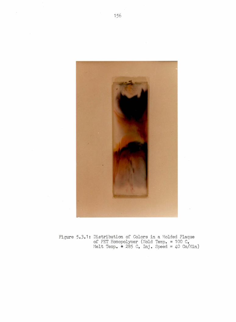
156
Figure 5.3.1: Distribution of Colors in a Molded Plaque of PET Homopolymer (Mold Temp. = 100 C, Melt Temp. * 285 C, Inj. Speed= 40 Cm/Min)


158
Figure 5.3.3: Longitudinal Section of Short-Shot type of Injection for 60 Hole % PHB/PET

Figure 5.3.4: Lon~itudinal Section of Short-Shot type of Injection for 80 Mole ~~ PHB/PET

FLOW FRONT
SOLIDIFYING RF...GION
=·.:·,~ ... -.. ~: .......... ··.· ~: .··;'. · .. , ... ;·.· • • ; .t. • •• ,. ' •• ·- • - • .. - • ••• •••• : ••• •• • ';• • ...... _ ,,.":' ...... , ...
. . .. . . . . .. ·. ·~:···· ·.'· .. :: ,: ): ::. · .. i- .. ··:·: • ....... .
FLOW DIRECTION
FLUID PIGMENT SPLITTING
Figure 5.3.5: Proposed Mold Filling Mechanism for PET/PHB Copolymer Systems
161
5.4 MOLECULAR ORIENTATION OF LIQUID CRYSTALLINE POLYMERS IN INJECTION MOLDING
Melt flow during the molding of ·plastics parts always
causes an orientation of macromolecules. This molecular or-
ientation influences significantly the properties of the
molding. The crack behavior, tendency to distort, corrosion
and shrinkage depend on this state of orientation (Menges
and Wubken, 1973). For liquid crystalline polymers, oriented
parts show highly anisotropic physical properties (Jackson
and Kuhfuss, 1976). This molecular orientation is due to
both the shear deformation of the melt and the flow front.
The last objective in this work is to qualitatively study
the molecular orientation generated during unidirectional
and radial types of flow. The first type of flow is thought
to result in anisotropic molecular orientation whereas the
second type of flow is thought to result in biaxial orienta-
ti on.
For unidirectional flow, the percent shrinkage of the mi-
crotomed samples as a function of distance from the surface
of the molded parts is shown in chapter 4 for 60 mole %
PHB/PET and 80 mole % PHB/PET. .All shrinkage data show a
negligible amount of shrinkage along the flow direction
whereas across to the flow direction, it is significantly
higher. To qualitatively confirm that no density change oc-
cured, the thfckness of the molded part was measured before

162
and after annealing. It was noticed that a 5 percent in-
crease in thickness results from the annealing process. The
shrinkage across to the flow direction shows a maximum peak
away from the surface of the parts. This maximum peak cor-
responds to high molecular orientation in the shear zone
layer which was discussed in chapter 2. This is not to say
that maximum orientation is found away from the surface of
molded part. According to Menges and Wubken (1973), the ab-
solute maximum orientation is always found at the surface,
since the oriented state is frozen immediately and no possi-
bility for relaxation exists. Away from the shear zone lay-
er, the percent of shrinkage decreases corresponding to less
orientation in the core.
For liquid crystalline polymer, the data in chapter 4
shows a higher shrinkage across the flow direction than that
along the flow direction. This is contrast to amorphous po-
lymer. For the latter type, higher shrinkage would be ob-
served along the flow than that of across to the flow. The
explanation for this phenomena may be found base on the work
by Joseph, Wilkes and Baird (1982). Basically, the polymer
melt of PET/PHB copolymers has been reported to be nonho-
mogenous (Zachariades et al., 1982; Meesiri et al., 1982;
Joseph et al., 1982). Using chemical etching technique on
the pressed film, Joseph et al. have shown that these copo-
163
lymers contain two phases: PET rich and PHB rich phase. For
copolymer of 60 and 80 mole % of PHB, the PHB rich phase ap-
pears to be more continuous than the PET rich phase (figure
5.4.1). They suggested that when the melt undergoes deforma-
tion, the PHB rich region would have a lower viscosity and
thus would orient along the flow and migrate towards the
surface of the injection molded parts while the more viscous
PET phase preferentially remains in the core (Joseph er al.,
1982). Since PHB segments are rigid, they do not relax much
upon annealing. Therefore, along the flow direction, the
maximum shrinkage peak close to the surface is absent.
Furthermore, since not much of shear deformation occurs in
the core and the PHB rich phase is found in the skin region,
negligible shrinkage of the microtomed sample (along the
flow direction) is observed. Consequently, the rest of the
discussion for unidirectional flow will only concern the
shrinkage across to the flow direction.
The effect of injection speed on molecular orientation
can be easily understood. With increasing injection speed,
higher force is applied and thus more oriented molecules
will immediately be frozen at the mold surface as a result
of the increases in rate of elongation and cooling rate.
Therefore, the relative maximum molecular orientation would
move to the surface. This is actually seen in figures 5.4.2

164
to 5.4.7. From these figures, the relative maximum shrinkage
corresponding to the molecular orientation of the shear zone
moves closer to the surface as the injection speed increas-
es. The fact that the magnitude of the relative maximum is
nearly the same at lower and higher injection speed is pro-
bably due to the combination of the relaxation process dis-
cussed above and the slow speed of injection (which is lim-
ited by the capability of the instrument). A lower injection
speed will result in a longer injection time and therefore a
thicker frozen layer. A higher injection speed will result
parts with higher molecular orientation along the flow. This
would give rise to anisotropic mechanical properties of the
molded parts.
The effect of gap thickness on molecular orientation can
be seen in figures 5.4.8 to 5.4.13. In these figures, the
across the flow shrinkage at the same injection speed and
different gap thickness is shown. Similar to the case of
higher injection speed, with constant injection speed, the
smaller the cavity thickness, the larger the rate of shear
deformation and the larger amount of heat removal will oc-
cur( for a smaller cavity). As a result, the thinner the fro-
zen layer will be and therefore, the relative maximum orien-
tation will move toward the surface as the cavity thickness
decreases. This is indeed observed in figures 5.4.8 to
5.4.13 for across the flow direction.
165
The discussion so far about the relative maximum
orientation beneath the surface of the molded parts may also
hold for the case of radial flow. Evidence can be seen in
figures 5.4.14 to 5.4.21. The effect of injection speed on
shrinkage of microtomed samples is shown in figures 5.4.14
to 5. 4. 17. With decreasing injection speed, the relative
maximum orientation (peak) moves toward the center of the
plaque due to a thicker frozen layer developed. The effect
of cavity thickness on the amount of shrinkage is shown in
figures 5.4.18 to 5.4.21. Similar to unidirectional case,
holding the injection speed constant and decreasing the cav-
ity thickness which lead to a larger amount of heat being
removed,. Therefore, the thinner frozen layer will be and the
relative maximum orientation will move toward the surface of
the molded parts.
The major difference between the shrinkage of parts re-
sulting from unidirectional and radial flow is that a signi-
ficant amount of shrinkage along the flow direction exists
in the radial flow case whereas it is negligible in the uni-
directional flow case. For radial flow, the radial velocity
for any type of incompressible fluid is:
Vr = V(r,z) (5.4.1)

166
The equation of continuity is:
\] • v = 0
Therefore:
= 0 and f (z)
r
The rate of deformation tensor becomes:
2 oVr ar
i = 0 -
0
2 Vr r
0
0
0
(5.4.2)
(5.4.3)
The diagonal components are related by the continuity equa-
tion (5.4.2):
d- Vr = - Vr O r r
(5.4.4)
The term on the left side of equation 5. 4. 4, )V,. , reflects or the amount of elongational strain generated along the flow
direction (r-direction). The term on the right side of the
167
equation (5.4.4), V..-. r reflects the amount of elongational
strain generated normal to the flow direction ( e -direc-
tion). These two terms would qualitatively be respossible
for the molecular orientation generated in redial flow. Ac-
cording to this equation 5.4.4, the degree of the molecular
orientation, hence the percent of shrinkage, should be in
the same order of magnitude for the flow direction and its
transverse direction (r and 6-directions respectively). In
the publication by Schmidt (1976), it was found that the ra-
dial flow beyond the entrance region can be described as a
combination of planar extension and simple shear whereas the
equation 5.4.4 only describes the planar extensioal flow be-
havior. Therefore, the magnitude of shrinkage is not the
same in the r and e-directions. Of course, more work must be
done to confirm this explanation.
In summary,from the shrinkage data shown in this section,
biaxial orientation has been generated in radial flow. The
amount of shrinkage in both the e and r-directions becomes
significant. This is the result of planar extension and
shear flow. Increasing injection speed or decreasing cavity
thickness would make the relative maximum shrinkage peak
move toward the surface as a result of higher deformation,
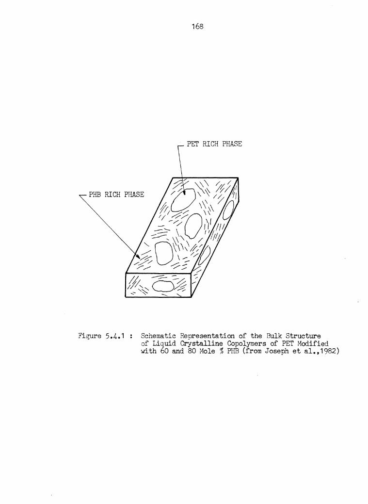
168
PET RICH PHASE
PHB RICH PHASE
Figure 5 .4. 1 Schematic Representation of the Bulk Structure of Liquid erYstalline Copolymers of PET Modified with 60 and 80 Hole % PHB (from Joseph et al., 1982)
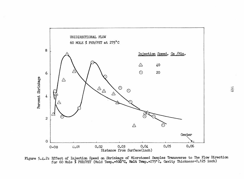
Q)
:f ~ ~ C>
~
8
6 6
4
2
UNIDIRECTIONAL FLOW 60 MOLE % PHB/PET at 275°C
0
Injection Speed, Cm /Min.
40
20
Center
O.__~~_._~~-'-~~~J__~~--'--~~---'-~~~~~----1 0·00 0.01 0.02 0.03 0.04
Distance from Sl.U"face(inch) 0.05 0.06
Figure 5.4.2: Effect of Injection Speed on Shrinkage of Microtomed Samples Transverse to 'lhe Fl.ow Direction for 60 Mole % PHB/PET (Mold Temp..=100°C, Melt Temp •. :;:275° C, Cavity 'lhiclmess==0.125 inch)
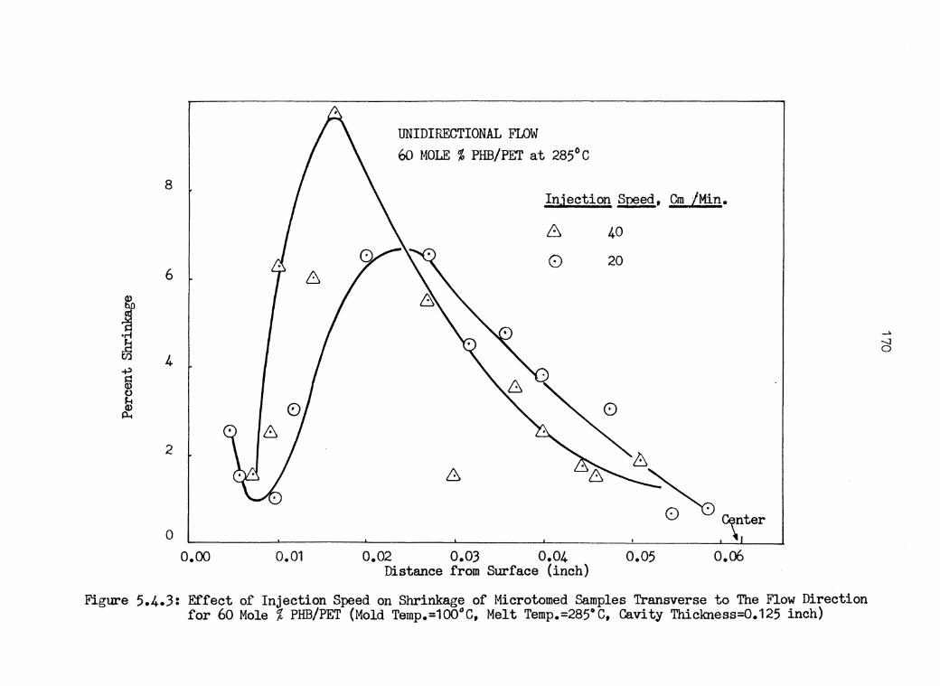
8
6
4
2
0 o.oo 0.01
UNIDIRECTIONAL FLOW 60 MOLE % PHB/PET at 285°C
Injection Speed, Cm /Min.
8
0
0.02 0.03 0.04 Distance from Surface {inch)
40
20
0
6
~~nter 0.05 o.06
Figure 5.4.3: Effect of Injection Speed on Shrinkage of Microtomed Samples Transverse to The Flow Direction for 60 Mole% PHB/PET {Mold Temp.=100°C, Melt Temp.=285°C, Cavity Thickness=0.125 inch)

UNIDIRECTIONAL FLOW 80 MOLE % PHB/PET at 305°C
8 Injection Speed, Cm /Min.
8 40
G 20 6
Q)
J 61 4 ~ w (.) J-f Q)
p.. 6 2
Center 0 \
o.oo 0.01 0.02 0.03 0.04 0.05 0.06 Distance from Surface (inch)
Figure 5.4.4: Effect of Injection Speed on Shrinkage of Microtomed Samples Transverse to The Flow Direction for 80 Mole % PHB/PET (Mold '.i.'emp.=100°C, Melt Temp.=305°C, Cavity 'l'hiclmess=0.125 inch)
..... -...J .....
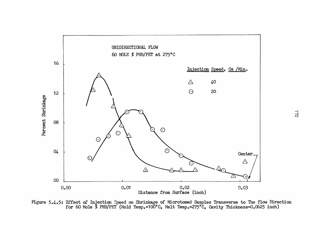
UNIDIRECTIONAL FLOW 60 MOLE % PHB/PET at 275°C
16 Injection Speed, Cm /Min.
~ 40
12 0 20 Q)
J ~ ~ 08 Q) 0 0 ~
04 c.ente7r 6
~ 00
o.oo 0.01 0.02 0.03 Distance from Surface (inch)
Figure 5.4.5: Effect of Injection Speed on Shrinkage of Microtomed Samples Transverse to The Flow Direction for 60 Mole % PHB/PET (Mold Temp.=100°C, Melt Temp.=275°C, Cavity Thickness=0.0625 inch)
_.. -..J I\)

16
12
08
00 o.oo
UNIDIRECTIONAL FLOW 60 MOLE % PHB/PET at 285°C
0.01
Injection Speed, Cm /Min.
0.02 Distance from Surface (inch)
Center
""' Figure 5.4.6: Effect of Injection Speed on Shrinkage of Microtomed Samples Transverse to The Flow D::;rection
for 60 Mole % PHB/PET (Mold Temp.=1004C, Melt Temp.=285°C, Cavity Thickness=0.0625 inch)

8
6
4
2
0 o.oo
UNIDIRECTIONAL FLOW 0 80 MOLE % PHB/PET at 305°C
Injection Speed, Qn/Min.
6 0
0.01
40 20
0.02 Distance from Surface(inch)
Cen~
0.03
Figure 5.4.?: Effect of Injection Speed on Shrinkage of Microtomed Samples Transverse to The Flow D:trection for 80 Mole % PHB/PET (Mold Temp.=100°C, Melt Temp.=305°C, Cavity Thickness=0.0625 inch)

UNIDIRECTIONAL FLOW 60 MOLE % PHB/PET at 275°C
8 Ca.vi ty Thickness, !!!9b.:
~ 0.1250 6 0 0.0625
4
2
Center 0 \
0.02 0.03 0.04 Distance from Surface (inch)
o.o 0.01 0.05 0.06
Figure 5.J,..8: Effect of Cavity Thickness on Shrinkage Transverse to The Fl.ow Direction for 60 Mole % PHB/PET (Mold Temp.= 100°C, Melt Temp.= 275°C, Injection Speed= 20 Cm/Min.)
..... -J
"'

UNIDIRECTIONAL FLOW 60 MOLE % PHB/PET at 2a5°c
16
Cavity Thickness, ~:
~ 0.1250 0 0.0625
4
Center
0 ·\ 0 o.o 0.01 0.02 0.03 0.04
Distance from Stn"face (inch) 0.06
Figure 5.4.9: Effect of Cavity Thickness on Shrinkage Transverse to The Flow Direction for 60 Mole % PHB/PET (Mold Temp.= 100°C, Melt Temp.= 285°C, Inject;Lon Speed= 20 Cm/Min.)
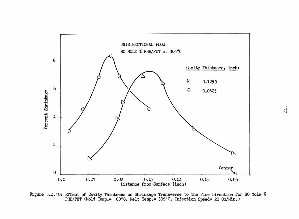
UNIDIRECTIONAL FLOW 80 MOLE % PHB/PET at 305°C
8
Cavity Thickness, ~:
~ 0.1250
0 0.0625
2
0 Cente~
o.o 0.01 0.02 0.03 0.04 0.05 o.o6 Distance from Surface (inch)
Figure 5.4.10: Effect of Cavity Thickness on Shrinkage Transverse to The Flow Direction for 80 Mole % PHB/PET (Mold Temp.= 100°C, Melt Temp.= 305°C, Injection Speed= 20 Cm/Min.)
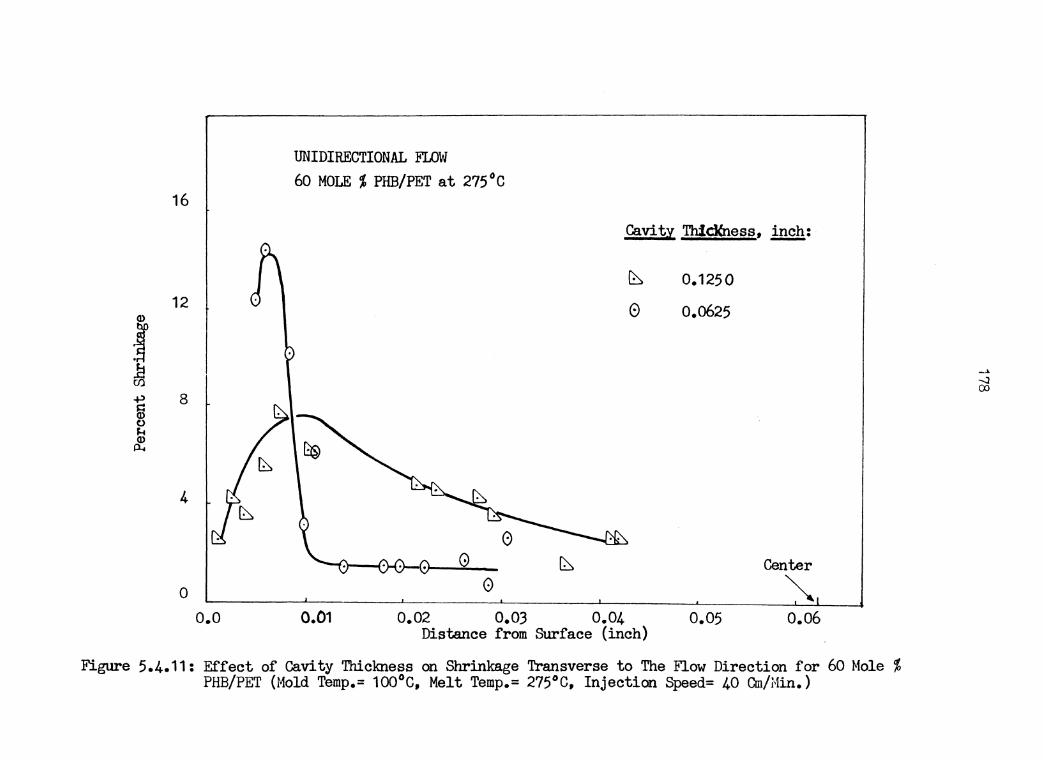
UNIDIRECTIONAL FLOW 60 MOLE % PHB/PET at 2?5°C
16
Ca.vi ty Thidmess, E.!£h:
~ 0.1250 12 0 0.0625
8
4
G Center 0 0 ~
o.o 0.01 0.02 0.03 0.04 0.06 Distance from Surface (inch)
Figure 5.4.11: Effect of Cavity Thickness on Shrinkage Transverse to The Flow Direction for 60 Mole % PHB/PET (Mold Temp.= 100°C, Melt Temp.= 2?5°C, Injection Speed= 40 Cm/Min.)
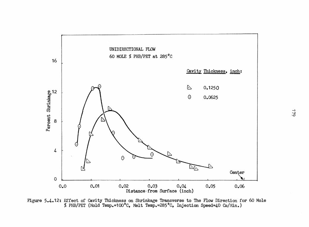
UNIDIRECTIONAL FLOW 60 MOLE % PHB/PET at 285°C
16
Cavity Thickness, ~:
~ 0.1250
0 0.0625
4 0
Center 0 ~
o.o 0.01 0.02 0.03 0.04 0.05 o.06 Distance 1from Surface (inch)
Figure 5.4.12: Effect of Cavity Thickness on Shrinkage Transverse to The Flow Direction for 60 Mole % PHB/PET (Mold Temp.=100°C, Melt Temp.=285°C, Injection Speed.=40 Cm/Min.)

UNIDIRECTIONAL FLOW
8 80 MOLE % PHB/PET at 305°C
Q) 6 Cavity Thiclmess, ~:
J ~ 0.1250 ~ 0 0.0625 ~ C) 4 ~
2
Center 0 ~
o.o 0.01 0.02 0.03 0.04 Distance from Surface (inch)
0.05 o.06
Figure 5.4.13: Effect of Cavity Thickness on Shrinkage Transverse to The Flow Direction for 80 Mole % PHB/PET (Mold Temp.=100°C, Melt Temp.=305°C, Injection Speed=40 Cm/Min.)
-' ()'.) 0

20
15
10
5
0 o.o 0.01
RADIAL FLOW 60 MOLE % PHB/PET at 275°c
Direction/Injection Speed
~ 9-direction, 40 Cm/Min.
0 r-direction, 40 Cm/Min.
~ 8-direction, 20 Cm/Min.
• r-direction, 20 Cm/Min.
0
Center \
0.02 0.03 0.04 0.05 0.06 Distance from Stn"face (inch)
Figure 5.4.14: Effect of Injection Speed on Shrinkage of Microtomed Samples for 60 Mole% PHB/PET (Mold Temp.= 165°C, Melt Temp.= 275°C, Cavity Thickness= 0.125 inch)
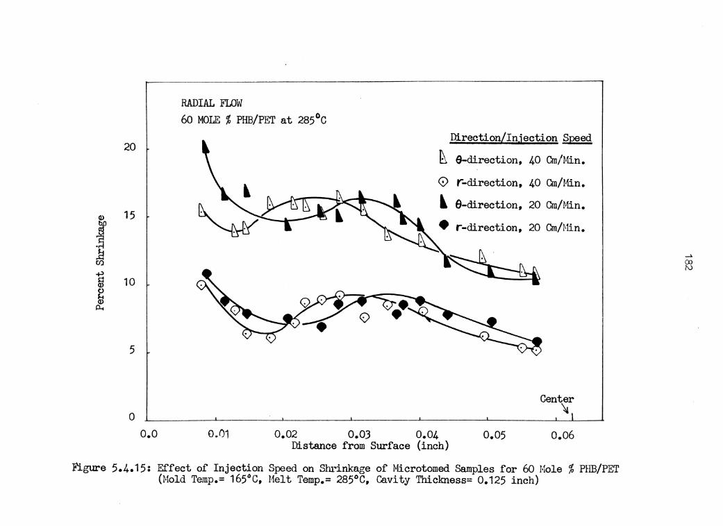
RADIAL FLOW 60 MOLE % PHB/PET at 285°C
DirectionLinjection S~ed
~ 6-direction, 40 Cm/Min. 20
0 r-direction, 40 Cm/Min.
l 6-direction, 20 Cm/Min.
• r-direction, 20 Cm/Min.
~
Q) 15 ~ J 1:! CJ)
fil 10 ()
~ p...
5
Center 0 ~
o.o 0.01 0.02 0.03 0.04 0.05 0.06 Distance from Surface (inch)
tigure 5.4.15: Effect of Injection Speed on Shrinkage of Microtomed Samples for 60 Mole % PHB/PET (Mold Temp.= 165°C, Melt Temp.= 285°C, Cavity Thiclmess= 0.125 inch)
__. (X) [\)

RADIAL FLOW 60 MOLE % PHB/PET at 275°C
Di.rectionlinjection S.el!ed
20 ~ 8-direction, 40 Cm/Min.
0 r-direction, 40 Cm/Min.
~ 8-direction, 20 Cm/Min •
j 15 • r-direction, 20 Cm/Min.
~ ~ ~ +> ti} 10 C> '-4 ~
• 5
• Center 0
o.o 0.01 0.02 0.03 Distance from Surface (inch)
Fig1..&re 5.4.16: Effect of Injection Speed an Shrinkage of Microtomed Samples for 60 Mole % PHB/PET (Mold Temp.= 165°C, Melt Temp.= 275°C, Cavity Thickness= 0.0625 inch)
_. 00 \..V

RADIAL FLOW 60 MOLE % PHB/PET at 285°C
20 Directionlinjection S~ed
~ 9-direction, 40 Cm/Min.
0 r-ctirection, 40 Cm/Min.
~ e-direction, 20 Cm/Min.
• r-ctirection, 20 Cm/Min. 15
10
~
5
0 Center
0 ~
o.o 0.03 0.01 0.02 Distance from Surface (inch)
Figure 5.4.17: Effect of Injection Speed on Shrinkage of Microtomed Samples for 60 Mole % PHB/PET (Mold Temp.= 165°C, Melt Temp.= 285°C, Cavity Thickness= 0.0625 inch)
__. 00 ~
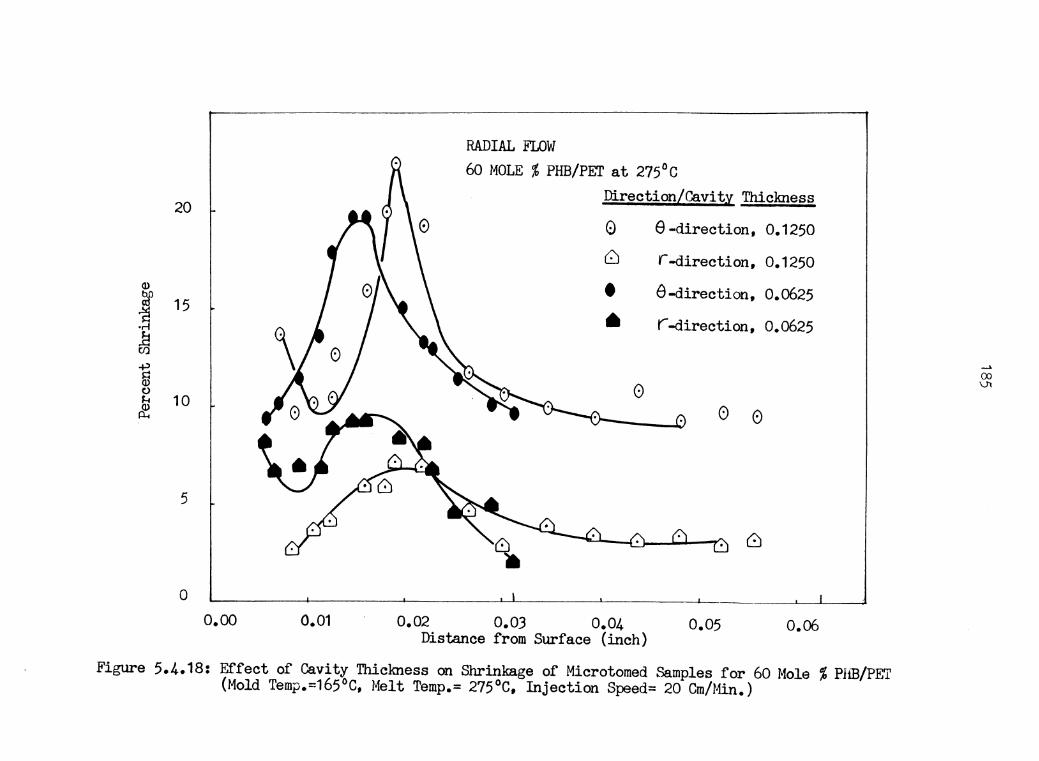
20
15
10
5
0 o.oo 0.01
RADIAL FLOW 60 MOLE % PHB/PET at 275°C
Direction/Cavity Thickness
0 e -direction, 0.1250 c;J r -direction, 0.1250
• e-ctirection, 0.0625 A r-ctirection, 0.0625
0 0 0
0.02 0.03 0.04 Distance from Surface (inch)
0.05 o.06
Figure 5.4.18: Effect of Cavity Thickness on Shrinkage of Microtomed Samples for 60 Mole % PHB/PET (Mold Temp.=165°C, Melt Temp.= 275°C, Injection Speed= 20 Cm/Min.)

20
15
10
5
0 o.oo 0.01
RADIAL FLOW 60 MOLE % PHB/PET at 285°C
0.02 0.03 0.04
Direction/Cavity Thickness
0 e -direction, o. 1250
~ r-direction, 0.1250
B-direction, 0.0625
r-direction, 0.0625
0.05 o.06 Distance from Surf ace (inch)
Figure 5.4.19: Effect of Cavity Thickness on Shrinkage of Microtomed Samples for 60 Mole % PHB/PET (Mold Temp.= 165°C, Melt Temp.= 285°C, Injection Speed= 20 Cm/Min.)

RADIAL FLOW 60 MOLE % PHB/PET at 275°C
20 Direction/Cavity Thickness
0 B-direction, 0.1250 c:'.:) r-direction, 0.1250
• 8-direction, 0.0625
A r-direction, 0.0625
5
0
o.oo 0.01 0.02 0.03 0.04 0.05 0.06 Distance from Surface (inch)
Figure 5~4.20: Effect of Cavity Thickness on Shrinkage of Microtomed Samples for 60 Mole % PHB/PET (Mold Temp.= 165°C, i"1elt Temp.= 275°C, Injection Speed= 40 Cm/Min.)
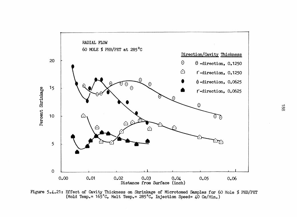
RADIAL FLOW 60 MOLE % PHB/PET at 285°C
DirectionLCavit~ Thickness 20 0 e -direction, 0.1250
~ r -direction, 0.1250
• e-direction, 0.0625
• r-direction, 0.0625
10
5
0 o.oo 0.01 0.02 0.03 0.04 0.05 o.06
Distance from Surface (inch)
Figure 5.4.21: Effect of Cavity Thickness on Shrinkage of Microtomed Samples for 60 Mole % PHB/PET (Mold Temp.= 165°C, Melt Temp.= 285°C, Injection Speed= 40 Cm/Min.)
Chapter VI
CONCLUSIONS
The dependence of viscosity on capillary diameters for
PET/PHB copolymer has been investigated. The mold filling
characteristics and molecular orientation in injection mold-
ing have been qualitatively studied. The following conclu-
sions may be drawn from the results of this work.
1. Unlike PET homopolymer, this liquid crystalline po-
lymer system is highly non-Newtonian and pseudoplas-
tic fluid. Increasing the degree of stiffness of the
polymer chain by increase the percentage of PHB con-
tent does not show a decrease in viscosity of the
melt as the 60 mole % PHB/PET copolymer shows lower
viscosity than the 80 mole % PHB/PET copolymer.
2. Melt viscosity of 60 mole% PHB/PET measured at 27S0 c shows a slight dependence on capillary diameter. This
is probably caused by a boundary layer of molecules
oriented parallel to the flow direction. At the
boundary, the viscosity of the melt is less than that
of the core fluid. For smaller capillary diameters,
the boundary occupies a greater percentage of the
flow channel. This explains the decrease in viscosity
with decrease in capillary diameter.
189
190
3. The reverse of the order of colors suggests that the
first material entering the mold would lay on the
wall and remained near the gate. The succeeding ma-
terial accelerates in the core, to the front, splits
and lays on the walls away from the gate.
4. Unlike amorphous polymers where the splitting pat-
terns only occur at the flow front, for liquid crys-
talline polymers, the splitting occurs even when the
fluid pigment is in the core. This splitting magni-
fies gradually and accelerate to the flow front. Upon
contacting with the cold wall, the splitting of the
fluid pigments stops and forms a "V" shape which has
the direction opposite to that of the flow.
5. The negligible amount of shrinkage along the flow di-
rection arises from the orientation of the PHB rich
region at the surf ace of the molded part and the much
less orientation of the PET region in the core. Upon
heating up to annealing temperature, the induced or-
ientation of PHB region relaxes more slowly than that
of flexible chain polymer. Also, the PET region in
the core is not oriented. Therefore, insignificant
amount of shrinkage along the flow direction is ob-
served.

191
6. For unidirectional flow, neglegible shrinkage along
the flow direction and low viscosity observed for li-
quid crystalline polymer suggest a high degree of mo-
lecular orientation developed along the flow direc-
tion during extrusion. Because of this orientation,
the molded parts possess anisotropic mechanical prop-
erties as reported by Jackson & Kuhfus (1976).
7. For radial flow, biaxial orientation was observed.
Flow beyond the gate region is a conmposi tion of
shear and planar extensional flow.
8. In general, maximum orientation due to shear zone
moves to the surface for higher injection speed and
smaller cavity thickness due to a larger rate of
shear deformation and the larger amount of heat remo-
val.

Chapter VI I
RECOMMENDATIONS
Based on the results of this work, the following is the
list of recommendations for future study in the area of pro-
cessing and rheology of copolyester of PET with p-hydroxy-
benzoic acid.
1. The behavior of viscosity for liquid crystalline po-
lymer at high shear rate should be investigated. This
can be done by measuring viscosity of these melt us-
ing capillaries with smaller diameters (i.e. !) =
0. 009 inch).
2. Since the molecular rotation of molecules in isotrop-
ic state is different from that of nematic mesophase,
further work should include NMR studies for the melts
at these states.
3. Future study should investigate the phase transition
of 60 mole % PHB/PET copolymer using differential
scanning calorimetry, X-ray diffraction, and electron
microscopy.
4. Since boundary layer effect occurs at 2 75° C for 60
mole % PHB/PET, injection molding in unidirectional
flow with the wall specially treated is a direct ap-
plication of the boundary layer.
192
193
5. Mold filling studies should be carried out at higher
injection speed for both radial and unidirectional
flow.
6. Center-gated type of injection should be further stu-
died with the lower plate rotating to further inves-
tigate the biaxial orientation of these copolymers.
7. Physical properties of each layer of injection molded
parts (from surface to core) should be measured both
along and across the flow directions to correlate
with the shrinkage data shown in this work.
BIBLIOGRAPHY
Atkins, R.J. "Poiseuille Flow of Liquid Crystals of The Nematic Type". Arch. Ration. Mech. Anal., 38 224, 1970a.
Atkins, R.J. and F.M. Leslie. "Couette Flow of Nematic Liquid". Quart. J. Mech. Appl. Math., 23, pt. 2, 53, 1970b.
Bagley, E.B. and A.M. Birks. "Flow of Polyethylene into a Capillary". J. of Appl. Phys., Vol. 31, No. 3, March 1960.
Bagley, E.B. and H.J. Duffey. "Recover Shear Strain and the Barus Effect in Polymer Extrusion". Trans. Soc. Rheo., 14:4, 545, 1970.
Bagley, E.B. "The Separation of Elastic and Plastic Effect in Polymer Flow". Trans. Soc. Rheo., 5, 355, 1961.
Baird, D.G. "Rheology of Polymer with Liquid Crystalline Order". Liquid Crystalline Order in Polymers, A. Blumstein, Ed., Academic Press, N.Y., 1978.
Ballenger, T.F. et al. "Polymer Melt Flow Instabilities in Extrusion: Investigation of the Mechanism and Material and Geometric Variables". Trans. Soc. Rheo., 15:2, 195-215, 1971
Ballenger, T.F. and J.L. White. "The Development of the Velocity Melts in a Reservoir Approaching a Capillary Die". J. Appl. Polym. Sci., Vol. 15, pp. 1949-1962, 1971.
Ballman, R.L., R.L. Kruse, and W.P. Taggart. "Surface Fracture in Injection Molding of Filled Polymers". Polym. Engr. Sci., Vol. 10, No. 3, May 1970.
Ballman, R.L. and H.L. Toor. "Orientation in Injection Molding". Modern Plastics, pp. 113-124, Oct. 1960.
Barrall II, E.M. "Thermodynamics of Mesophase Transitions". Liquid Crystals: The Fourth State of Matter, F.D. Saeva, Ed., Marcel Dekker, Inc., N.Y., 1979.
Barrall II, E.M., R.S.Porter and J.F. Johnson. "Heats of Transition for Nematic Mesophases". Jour. of Phys. Chem. 68, 2810(1964).
194
195
Benbow, J.J. and P. Lamb. "New Aspect of Melt Fracture". SPE Trans., pp 7-17, Jan. 1963.
Berger, J.L. and C.G. Gogos. "A Numerical Simulation of the Cavity Filling Process with PVC in Injection Molding". Polym. Engr. Sci., Vol. 13, No. 2, March 1973.
Berreman, P.W. "Alignment of Liquid Crystals by Grooved Surfaces". Mol. Cryst. Liq. Cryst., 22, 215, 1973.
Bird, R.B. "Useful Non-Newtonian Models". Annual Review of Fluid Mechanics, Vol. 8, 1976.
Bird, R.B., P. Hassager and R.C. Armstrong. Dynamics of Polymeric Liquids, Vol. 1, John Wiley & Sons, Inc.,lil.Y., 1977.
Bird, R.B., M.W. Johnson, Jr., and J.F. Stevenson. "Molecular Theories of Elongational Viscosity".Proc. of the fifth Congr. on Rheology, Vol.4,S. Onogi, Ed. University of Tokyo, 1970, p.159.
Blumstein, A and E.C. Hsu. "Liquid Crystalline Order in Polymers with Mesogenic Side Groups". Liquid Crystalline Order in Polymers, A. Blumstein, Ed., Academic Press, N.Y., 1978.
Blyler Jr.,L.L. and T.W. Haas. "The Influence of Intermolecular Hydrogen Bonding on the Flow Behavior of Polymer Melts". J. Appl. Polym. Sci., 13, 2721, 1969.
Breyer, E., Z. Tadmor and C. Gutfinger. "Filling of a Rectangular Channel with a Newtonian Fluid". Israel J. Tech., Vol. 11, No. 4, 1973, pp.189-193.
Broyer, E., c. Gutfinger and Z. Tadmor. "A Theoretical Model for the Cavity Filling Process in Injection Molding". Trans. Soc. Rheo., 19:3, 423-444, 1975.
Casale, A., Moroni A. and I. Ronzoni. "An Approach for the Processing Engineer: Rheotechnics". Polym. Engr. Sci., 14:9, 651-55, Sept. 1974.
Chan, Y., J.L. White and Y. Oyanagi. "Influence of Glass Fiber on the Extrusion and Injection Molding Characteristics of Polyethylene and Polystyrene Melts". Polym. Engr. Sci., 18:4, 268-72, March 1978.

196
Chistyakov, I. "Ordering and Structure of Liquid Crystals". Advances in Liquid Crystals, Vol. l, G.H. Brown, Ed., Academic Press, N.Y., 1975.
Currie, P.K. "Viscometric Flows of Anisotropic Fluids". Rheo. Acta., 16:2, 205, 1977.
Currie, P.K. "Aproximate Solutions for Poiseuille Flow of Liquid Crystals". Rheo. Acta., 14:8, 688, 1975.
Currie, P.K. "Static Solutions with Phase Change for a Nematic Liquid Crystal in a Pipe". Trans. Soc. Rheo., 17:2, 197, 1973.
De Gennes, P.G. The Physics of Liquid Crystals, Claredon Press, Oxford, 1974.
De Gennes,P.G., P. Pincus. "Nematic Polymers". Polym. Prepr. 18, 161(1977).
Dietz, W., J.L. White and E.S. Clark. "Orientation Development and Relaxation in Injection Molding of Amorphous Polymers". Polym. Engr. Sci., Report No. 103, June 1977.
Duffy, B.R. "Flow of a Liquid with an Anisotropic Tensor: Some Axisymmetric Flows". Journal of Non-Newtonian Fluid Mechanics, 7 (1980) 359-367.
DuPre, D.B, E.T. Samulski and A.V. Tobolsky. "The Mesomorphic State: Liquid and Plastic Crystals." Polymer Science and Materials, A.V. Tobolsky and H.F. Mark, Wiley - Intersciences, N.Y., 1974
Duvdevani, I.J. and I. Klein. "Analysis of Polymer Melt Flow in Capillaries Including Pressure Effects". SPE Journal, 41-45, Dec 1967.
Ericksen, J.L. "A Boundary-Layer Effect in Viscometry of Liquid Crystals". Trans. Soc. Rheo., 13:1, 9, 1969a.
Ericksen, J.L. "Continuum Theory of Liquid Crystals of Nematic Type". Mol. Cryst. Liq. Cryst., 7, 153, 1969b.
Ericksen, J.L. "Conservation Laws for Liquid Crystals". Trans. Soc. Rheo., 5, 23, 1961.
197
Faulkner, E.L. and L.R. Schmidt. "Glass Bead-Filled Polypropylene Part 1: Rheological and Mechanical Properties". Report No. 76CRD200, Corporate Research and Developement, Schenectady, New York, Aug 1976.
Fisher, J. and A.G. Fredrickson. "Interfacial Effects on the Viscosity of a Nematic Mesophase". Mol. Cryst. Liq. Cryst., 8, 267, 1969.
Flory, P.J. and G. Ronca. "Theory of Systems of Rodlike Particles, II. Thermotropic Systems with Orientation-Dependent Interactions". Mol. Cryst. Liq. Cryst., 54, 311, 1979.
Gallet, B. "Liquid Crystalline Structure of Block Copolymers". Liquid Crystalline Order in Polymers, A. Blumstein, Ed., Academic Press, N.Y., 1978.
Goldblatt, P.H. and R.S. Porter. "A Comparison of Equations for the Effect of Pressure on the Viscosity of Amorphous Polymers". J. Appl. Polym. Sci., Vol. 20, 1199-1208, 1976.
Grover M.K., R. Zwanzig. "Polymer Concentration Effects on Helix-Coil Transition Widths". Biopolymers 13, 2103(1974).
Han, C.D. "Stress Birefringence Patterns in Molten Polymers During the Mold-Filling and Cooling Process". J. Appl. Polym. Sci., Vol. 18, 3581-3592, 1974.
Han, C.D. "On Silt- and Capilarry Die- Geometry''. Trans. Soc. Rheo., 18:1, ·163-190, 1974.
Han, C.D. Rheology in Polymer Processing, Academic Press, N.Y., 1976.
Han, C.D. and M. Charles. ''Entrance- and Exit-Correction in Capillary Flow Molten Polymers". Trans. Soc. Rheo., 15:2, 371, 1971.
Han, C.D., M. Charles, and W. Philippoff. "Measurement of the Axial Pressure Distribution of Molten Polymers in Flow Through a Circular Tube". Trans. Soc. Rheo., 13:4, 455-466, 1969.
198
Han, C.D., M. Charles, and W. Philippoff. "Rheological Implications of the Exit Pressure and Die Swell in Steady Capillary Flow of Polymer Melts. I. The Primary Normal Stress Difference and the Effect of L/D Ratio on Elastic Properties". Trans. Soc. Rheo., 14:3, 409, 1970.
Han, C.D., C.A. Villamiza, and Y.W. Kim. "Morphology and Mechanical Properties of Injection-Molded Specimens of TwoPhase Polymer Blends". J. Appl. Polym. Sci., Vol. 21, 353- 370, 1970.
Harry, D.H. and R.G. Parrott. "Numerical Simulation of Injection Mold Filling". Polym. Engr. Sci., 10:4, 209-214, July 1970.
Jackson, G.B. and R.L. Ballman. "The Effect of Orientation on the Physical Properties of Injection Moldings". SPE Journal, 1147-1152, Oct 1960.
Jackson, Jr. W.J. and H.F. Kuhfuss. "Liquid Crystal Polymers. I. Preparation and Properties of p-hydroxybezoic Acid Copolymers". J. Polym. Sci., 14, 2043, 1976.
Jenkins, J.T. "Flows of Nematic Liquid Crystals". Ann. Rev. Fluid Mech., 10, 197, 1978.
Jerman, R.E. "A Rheological Characterization of Liquid Crystalline Copolymers of Poly (ethylene Terephthalate) ", V.P.I & S.U. Thesis, 1980.
Jerman, R.E. and D.G. Baird. "Rheological Properties of Copolyester Liquid Crystalline Melts. I. Capillary Rheometry". J. Rheo., 25(2), 275-292, 1981.
Joseph, E., G.L. Wilkes and D.G. Baird. "Morphological Study of Thermotropic Liquid Crystalline Polyesters Based on PET and p-hydroxy Bezoic Acid.", in printing.
Kamal, M.R. and S. Kenig. "The Injection Molding of Thermoplastics Part I: Theoretical Model". Polym. Engr. Sci., 12:4, 294-301, July 1972.
Kamal, M.R. and S. Kenig. "The Injection Molding of Thermoplastics Part II: Experimental Test of the Model". Polym. Engr. Sci., 12:4, 302-308, July 1972.
Kamal, M.R., Y. Kuo and P.H. Doan. "The Injection Molding Behavior of Thermoplastics in Regtangular Cavities." ibid., 15, 863(1975)
199
Kamal, M.R. and H. Nyun. "Capillary Viscometry: A Complete Analysis Including Pressure and Viscous Heating Effects". Polym. Engr. Sci., 20:2, 109-119, Jan 1980.
Kamal, M.R., Y. Kuo. "The Fluid Mechanics and Heat Transfer of Injection Mold Filling of Thermoplastic Materials". AIChe J., 22:4, 661-669, July 1976.
Kantz, M.R. , H.D. Newman and F.H. Stigale, J. Appl. Polymer Sci. , 16, 1249(1972).
Kim, Y.H. and P. Pincus. "Nematic Polymers: Excluded-Volume Effects". Biopolymers 18, 2315(1979).
Laurencena, B.R. and M.C. Williams. "Radial Flow of No'n-Newtonian Fluids Between Parallel Plates". Trans. Soc. Rheo., 18:3, 331-355, 1974.
Lee, B.L. and J.L. White. "An Experimental Study of Rheological Properties of Polymer Melts in Laminar Shear Flow and of Interface Deformation and Its Mechanisms in Two-Phase Stratified Flow". Trans. Soc. Rheo., 18:3, 467-492, 1974.
Leslie, F.M. "Some Constitutive Relations for Liquid Crystals". Arch. Ration. Mech. Anal., 28, 265, 1968.
Leslie, F.M. "Continuum Theory of Cholesteric Liquid Crystals". Mol. Cryst. Liq. Cryst., 7, 407, 1969.
Leslie, F.M. "Theory of Flow Phenomena in Liquid Crystals". Advances in Liquid Crystals, Vol. 4, G.H. Brown, Ed., Academic Press, N.Y., 1979.
McFarlane, F.E., V.A. Nicely and T.G. Davis. "Liquid Crystal Polymers. II. Preparation and Properties of Polyesters Exhibiting Liquid Crystalline Melts." Contemporary Topics in Polymer Science, Vol. 2, E.M. Pearce and J.R. Schaefgan, Ed., Plenum Publishing Corp., N.Y., 1977.
McLuckie, C. and M.G. Rogers. "Influence of Elastic Effects on Capillary Flow of Molten Polymers". J. Appl. Polym. Soc., Vol. 13, 1049-1062, 1969.
Meesiri, W. et al. "Phase Transitions in Mesophase Maromolecules. III. The Transitions in Poly (ethylene Terephthalate-co-p-oxybenzoate) ". J. Polym. Sci.: Polymer Physics Edition, Vol. 20, 719-728, 1982.

200
Meissner, J. "Capillary Rheometry for Polymer Melts". Rheology of Polymeric Liquids, Von Karman Institute for Fluid Dynamics, Rhode Saint Genese, Belgium, 1978.
Menges, G. and G. Wubken. "Influence of Processing Conditions on Molecular Orientation in Injection Moldings", Annual Technical Conference of the Soc. of Plastics Eng. Preprints, Montreal, Canada, 1973, p.519
Metzger, A.P., C.W. Hamilton and E.H. Merz. "Anomalous Flow Behavior of High Density Polyethylene Melts". SPE Trans., 21-26, Jan 1963.
Metzger, A.P. "Extensional Primary Field Approximations for Viscoelastic Media". Rheo. Acta., 10, 434-444, 1971
Middleman, S. The Flow of High Polymers, Wiley-Interscience, N.Y., 1968.
Middleman, S. Fundementals of Polymer Processing, McGraw Hill, N.Y., 1977.
Morgan,P.W. "Synthesis and Properties of Aromatic and Extended-chain Polyamides." Poly, Prepr. Div. of Poly. Chem., Am. Chem. Soc., 17:1, 47, 1976.
Moss, E.A. "Flow Visualisation Techniques". The South African Mechanical Engineer, Vol. 30, 84-89, Mar 1980.
Oda, K., J.L. White and E.S. Clark. "Jetting Phenomena in Injection Mold Filling". Polym. Engr. Sci., 16:8, 585, Aug 1976.
Ohgawara, M., T. Uchida and M. Wada. "Liquid Crystal Orientation on Various Surfaces". Mel. Cryst. Liq. Cryst., Vol. 74, 227-242, 1981.
Okubo, S. and Y. Hori. "Shear Stress at Wall and Mean Normal Stress Difference in Capillary Flow of Polymer Melts". J. Rheo., 23:5, 625-649, 1979.
Onogi, Y., J.L. White and J.E. Fellers. "Rheo-Optics of Shear and Elongational Flow of Liquid Crystalline Polymer Solutions: Hydroxypropyl Cellulose/Water and Poly p-phenylene Terephthalamide/Sulfuric Acid". Journal of Non-Newtonian Fluid Mechanics, 7, 121-151, 1980.
201
Papkov, S.P., V.G. Kulichikhin, V.D. Kalmykova and A.Y. Mackin. "Rheological Properties of Anisotropic Poly (p-benzamide) Solutions". J. Polym. Sci. , Polym. Phys. Ed. , 12, 1753, 1974.
Philippoff, W. and F.H. Gaskins. "The Capillary Experiment in Rheology". Trans. Soc. Rheo., II, 263- 284, 1958.
Porter, R.S., E.M. Barrall, II, and J.F. Johnson. "Some Flow Characteristics of Mesophase Types". J. Chem. Phys., 45, 1452 ( 1966).
Porter, R.S. and J.F. Johnson. "The Rheology of Liquid Crystals". Rheology, Theory and Application, Vol. 4, F.R. Elrich, Ed., Academic Press, N.Y. 1967.
Preston, J. "Synthesis and Properties of Rodlike Condensation Polymers". Liquid Crystalline Order in Polymers, A. Blumstein, Ed., Academic Press, N.Y., 1978.
Rajan V.T. and C.W. Woo. "Liquid Crystalline Properties and reeentrance Phenomena in PBLG solutions". Phys. Rev. A2 l , 9 9 0 ( 19 8 0 ) .
Richardson, S. "Hele Shaws Flows with a Free Boundary Produced by the Injection of Fluid into a Narrow Channel". J. Fluid Mech., 56:4, 609-618, 1972.
Saeva, F.D. "Nematic Mesophases". Liquid Crystal: The Fourth State of Matter, F.D. Saeva, Ed., Marcel Dekker, Inc., N.Y., 1979.
Sakiadis, B.C. "Equilibrium Flow of a General Fluid Through a Cylindrical Tube". AIChe J., 8:3, 317-321, Jul 1962.
Samulski, E.T. "Polymeric Liquid Crystals". Physics Today, May 1982, 40-46.
Saupe, A. "On Molecular Structure and Physical Properties of Thermotropic Liquid Crystals." Mol. Crys. Liq. Crys., 7, 59, 1969.
Schmidt, L.R. "A Special Mold and Tracer Technique for Studying Shear and Extensional Flows in a Mold Cavity During Injection Molding". Polym. Engr. Sci., 14:11, 797-800, Nov 1974.
Schmidt, L.R. "Diverging Radial Flow of Glass Bead-Filled Polypropylene Between Parallel Plates". Report No. 76CRD202, Cor. Res. Dev., Aug 1976.
202
Schmidt, L.R. "Experimental Studies of Injection Mold Filling". Report No. 77CRD142, Corp. Res. Dev., Jun 1977.
Shiboyev, V.P. and N.A. Plate. "Liquid Crystalline Polymers". J. Polym. Sci., 19:5, 923, 1977.
Sleeman, M.J. and G.H. West. "Runner Flow in Injection Moulds". Br. Polym. J., 1973, 5, 91-99.
Spencer, R.S. and G.D. Gilmore. "Some Flow Phenomena in the Injection Molding of Polystyrene". Presented at the Annual Meeting of the Society of Rheology, New York, N.Y., Nov 3-4, 1950.
Tadmor, Z. "Molecular Orientation in Injection Molding". J. Appl. Polym. Sci., 18, 1753, 1974.
Tadmor, Z. and C.G. Gogos. Principles of Polymer Processing, Wiley-Interscience, N.Y., 1979.
Thienel, P. and G. Menges. "Mathematical and Experimental Determination of Temperature, Velocity, and Pressure Fields in Flat Molds During the Filling Process in Injection Molding of Thermoplastics". Polym. Engr. Sci., 18:4, 314-320, Mar 1978.
Toor, H.L., R.L. Ballman and L. Cooper. "Predicting Mold Flow by Electronic Computer". Modern Plastics, Dec 1960, 117-209.
Tsvetkov, V.N., E.I. Rjumtsev, and I.N. Shtennikova. "Intramolecular Orientation Order and Properties of Polymer Molecules in Solution." Liquid Crystalline Order in Polymers, A. Blumstein, Ed., Academic Press, N.Y., 1978.
Van Der Wielen, M.P. "The Flow Behavior and Impact Strengh of Poly (buthylene-terephthalate) as a Functio,n of Several Processing Variables". Polym. Engr. Sci., 15:2, 102, Feb 1975.
Wales, J.L.S., IR J. Van Leeuwen and R. Van Der Vijgh. "Some Aspects of Orientation in Injection Molded Objects". Polym. Engr. Sci., 12:5, 358-363, Sep 1972.
Wampler, F.C., D.R> Gregory and W.D. Kennedy. "Spinning of Poly (ethylene-terephthalate) Fibers from a Melt Pool Without a Spinneret". J. Appl. Polym. Sci., 16, 99-106, 1972.

203
Wendorff, J.H. "Scattering in Liquid Crystalline Polymer Systems". Liquid Crystalline Order in Polymers, A. Blumstein, Ed., Academic Press, N.Y., 1978.
White, J.L. "Fluid Mechanical Analysis of Injection Mold Filling". Polym. Engr. Sci. , 15: 1, 44-50, Jan 1975.
White, J.L. "Fluid Mechanical Analysis of Injection Mold Filling". Report No. 24 (revised). Dept. Chem. and Mettalurgical Engr., Univ. Tenn.
White, J.L. and H.B. Dee. "Flow Visualisation for Injection Molding of Polyethyene and Polystyrene Melts". Polym. Engr. Sci., 14:3, 212-222, Mar 1974.
White, J.L. and B.L. Lee. "An Experimental Study of Sandwith Injection Molding of Two Polymer Melts Using Simultaneous Injection". Polym. Engr. Sci., 15:7, 481-485, Jul 1975.
White, J.L., K. Oda, E.S. Clark and Y. Yonezawa. "Rheological Phenomena in Injection Molding". Dept. Chem. and Mettalurgical Engr., Univ. Tenn.
Williams, G. and H.A. Lord. "Mold-Filling Studies for the Injection Molding of Thermoplastic Material. Part I: The Flow of Plastic Materials in Hot- and Cold-Walled Circular Channels". Polym. Engr. Sci., 15:8, 553-568, Aug 1975.
Williams, G. and H.A. Lord. "Mold-Filling Studies for the Injection Molding of Thermoplastic Material. Part II: The Transient Flow of Plastic Materials in the Cavities of Injection-Molding Dies". Polym. Engr. Sci., 15:8, 569-582, Aug 1975.
Wissbrun, K.F. "Observations on the Melt Rheology of Thermotropic Aromatic Polyesters". Celanese Research Company, Summit, N.J., British Polym. J., 12(4), 163(1980)
Wissbrun, K.F. "Rheology of Rod-like Polymers in the Liquid Crystalline State." Jour. of Rheology, in printing.
Wu, P.C., C.F. Huang and C.G. Gogos. "Simulation of the Mold-Filling Process". Polym. Engr. Sci., 14:3, 223-230, Mar 1974.
204
Young, S.S., J.L. White, E. Clark and Y. Oyanagi. "A Basic Experimental Study of Sandwich Injection Molding with Sequential Injection". Polym. Engr. Sci. , 20: 12, 798-804, Aug 1980.
Zachariades, A.E., J. Economy and J.A. Logan. "The Morphology of the Aromatic Copolyester of PET and 80 mol% of p-Acetoxybenzoic Acid". J. Appl. Polym. Sci., Vol. 27, 2009-2014, 1982.

Appendix A
COMPUTER PROGRAM FOR VISCOSITY CALCULATION
Comment: c
This program is to calculate the viscosity of polymer melt from the raw data of Instron capillary rheometer model 3211. Entrance pressure loss is also calculated from the linear regression of total pressure drop vs L/D ratio (Bagley plot). Corrected wall shear stress and wall shear rates are thus obtained.
c c c c c c c c c c c c c c
c c c c c c c
c
1 100
101
2
5 6
3
Input: Speed of Plunger and Pressure readings for capillaries with different L/D ratio.
Output: Entrance pressure loss, corrected Wall Shear Stress, Apparent Shear Rate, Wall Shear Rate and Viscosity.
REAL D,TEMP,L(10),SPEED(l8),FORCE(18),LNGAMA(l8) REAL LNPRES(18),C(ll),LNTW(6,30),LNTWS(30) REAL APGAMA(30),PRESS(6,30),RATI0(6),PEN(30),TW(6,30) REAL LNAPGA(30), GAMAW(6,30),ETA(6,30),APRESS(6) REAL FORCES(l8,4),AGAMA(18),PRESUR(l8,4),PRESSE(30,6) INTEGER N,NDATA(18),DATA,M,K,I,S,Y INTEGER DOTS(4,130),DOT,POLYMA,POLYMB,POLYMC DATA DOT/lH*/
The data is input here: N = number of capillary, i.e. 03 D = Capillary Diameter TEMP = Melt Temperature POLYMA, POLYMB, POLYMC = name of polymer
READ (5,100) N,D,TEMP,POLYMA,POLYMB,POLYMC FORMAT (I2,lX,F7.5,lX,F5.l,lX,3A4) IF (N .EQ. 0) GOTO 600 WRITE (6,101) FORMAT (lHl) DO 6 I=l,4 DO 2 J=l,130 DOTS(I,J)=DOT CONTINUE WRITE(6,5) (DOTS(I,J),J=l,130) FORMAT(lX,130Al) CONTINUE WRITE (6,7) WRITE (6,3) POLYMA, POLYMB, POLYMC, TEMP, D FORMAT (lX, 'RHEOLOGICAL PROPERTY OF I ,3A4, 'AT I ,FS.l,lX,
+' DEGREE CENTIGRADE' ,SX, 'CAPILLARY DIAMETER= ',F7.5)
205
206
C Input of Raw Data: C L(I) = Length of capillary (inch) C NDATA(I) = number of data points C SPEED(J) = speed of plunger (cm/min) C FORCE(J) = Pressure reading (kg) c
DO 40 I=l,N READ (5,200) L(I),NDATA(I) DATA= NDATA(I) DO 10 J=l,DATA READ (5,300) SPEED(J), FORCE(J) FORCES(J,I)=FORCE(J)
10 CONTINUE c C Calculation of apparent shear rate and total pressure C drop from raw data c
DO 20 K=l,DATA AGAMA(K)=2.0*SPEED(K)*((0.9525)**2)/(15.0*(((D*2.54)**3))) LNGAMA(K)=ALOG(AGAMA(K)) PRESUR(K,I)=(l.375E05)*FORCE(K) LNPRES(K)=ALOG(PRESUR(K,I))
20 CONTINUE c C Using linear least square to compute entrance pressure C loss from Bagley Plot c
CALL LEAST (LNGAMA,LNPRES,l,C,DATA) APGAMA(l)=lO.O DO 30 M=l,28 LNAPGA(M)=ALOG(APGAMA(M)) PRESS(I,M)=EXP((C(2))*LNAPGA(M)+C(l)) PRESSE(M,I)=PRESS(I,M) IF (APGAMA(M).LT.100.0) GOTO 22 IF (APGAMA(M).LT.1000.0) GOTO 24 IF (APGAMA(M).LT.10000.0) GOTO 26 GO TO 31
22 S=M+l APGAMA(S)=APGAMA(M)+lO.O GO TO 30
24 S=M+l APGAMA(S)=APGAMA(M)+lOO.O GO TO 30
26 S=M+l APGAMA(S)=APGAMA(M)+lOOO.O
30 CONTINUE 31 DO 40 Y=l,11
C(Y)=0.0 40 CONTINUE
WRITE (6,7) DO 60 M=l,28 DO 50 I=l,N RATIO(I) = L(I)/D
50 APRESS(I) = PRESS(I,M)

c
207
CALL LEAST (RATIO,APRESS,l,C,N) PEN(M) = C(l) DO 60 J=l,11 C(J) = 0.0
60 CONTINUE WRITE (6,45) (RATIO(I),I=l,3)
45 FORMAT (lX, 'SPEED*******FORCE, L/D = I ,6(2X,F6.2)/) WRITE (6,46)
46 FORMAT (lX, I (CM/MIN)' ,4X, I (KG)'//) DO 41 J=l,DATA WRITE(6,42) SPEED(J),(FORCES(J,I),I=l,N)
42 FORMAT (1X,F4.l,4(5X,F7.2)/) 41 CONTINUE
WRITE (6,7) WRITE (6,47) (RATIO(I),I=l,3)
47 FORMAT (lX, 'APGAMA*******PRESSURE, L/D = I ,6(2X,F6.2)/) WRITE (6,48)
48 FORMAT (lX, I (SEC-1)' ,6X, I (KG/M.SEC2)'//) DO 44 J=l,DATA WRITE(6,43) AGAMA(J),(PRESUR(J,I),I=l,N)
43 FORMAT (1X,F7.l,4(5X,Ell.4)/) 44 CONTINUE
C Write apparent shear rate, total pressure drop for C each capillary and entrance pressure loss. c
c
WRITE (6,7) WRITE (6,66) (RATIO(I),I=l,3)
66 FORMAT (lX, 'APGAMA******PRESSURE, L/D = I ,3(2X,F6.2),3X, +'PRESS. ENTRANCE '/)
WRITE (6,67) 67 FORMAT (lX, I (SEC-1)' ,6X, I (KG/M.SEC2)' ,33X, '(KG/M.SEC2)'//)
DO 64 J=l,28 WRITE (6,63) APGAMA(J),(PRESSE(J,I),I=l,N),PEN(J)
63 FORMAT (1X,F7.l,5(5X,Ell.4)/) 64 CONTINUE
WRITE (6,7) 7 FORMAT(lX,' '//////)
C Calculation of corected wall shear stress from total C pressure drop and entrance pressure loss c
DO 80 I=l,N WR I TE ( 6 I 3 5 0 ) I WRITE (6,400) WRITE (6,450) DO 61 M=l, 28 TW(I,M)=(PRESS(I,M)-PEN(M))*D/(4.0*L(I)) LNTW(I,M)=ALOG(TW(I,M)) LNAPGA(M}=ALOG(APGAMA(M))
61 CONTINUE DO 65 S=l,28 LNTWS(S)=LNTW(I,S)
65 CONTINUE
208
DATA = 28 c C Using Linear least square to compute the power law C index of the polymer c
CALL LEAST (LNAPGA,LNTWS,l,C,DATA) c C Calculation of corrected wall shear rate and its C corresponding viscosity c
c c c c c
c c c c c
70
80 200 300 350
400
450
500
600
DO 70 M=l,28 GAMAW(I,M)=((3.0*C(2)+1.0)/(4.0*C(2)))*APGAMA(M) ETA(I,M)=TW(I,M)/GAMAW(I,M)
Print output: Pressure entrance, Wall shear stress, Apparent shear rate, corrected wall shear rate and Viscosity
WRITE (6,500) PEN(M),TW(I,M),APGAMA(M),GAMAW(I,M),ETA(I,M) CONTINUE DO 80 J=l,11 C(J)=O.O CONTINUE FORMAT (F5.3,1X,I2) FORMAT (F5.2,F7.2) FORMAT(lHl,lX, 'THE CALCULATED RHEOLOGICAL PROPERTIES ',
+I USING CAPILLARY' I I2, lX, I ARE: I//) . FORMAT(lX, 'ENTRANCE PRESSURE' ,13X, 'WALL SHEAR STRESS' ,13X,
+'APPARENT SHEAR' ,13X, 'WALL SHEAR RATE' ,13X,' VISCOSITY') FORMAT(lX, 'LOSS (KG/M.SEC2)' ,16X, I (KG/M.SEC2)' ,16X,
+'RATE (SEC-1)' ,19X, I (SEC-1)' ,17X, I (PASCAL.SEC)'//) FORMAT(4X,Ell.4,19X,Ell.4,21X,F7.l,22X,F8.2,18X,F8.2) GOTO 1 STOP END
This subroutine is to calculate the slope and y-intercept of a straight line from a set of data using the linear least square method
SUBROUTINE LEAST (X,Y,M,C,DATA) DIMENSION X(200),Y(200),A(ll,ll),B(ll),C(ll),P(20) INTEGER DATA NUMBER = DATA MX2 = M*2 DO 13 I=l,MX2 P(I) = 0.0 DO 13 J=l,NUMBER
13 P(I) = P(I)+X(J)**I N = M+l DO 30 I=l,N DO 30 J=l,N K =I+J-2 IF(K) 29,29,28
28 A(I,J) = P(K) GO TO 30
29 A(l,l) =NUMBER 30 CONTINUE
B(l) = 0.0 DO 21 J=l,NUMBER
21 B(l) = B(l)+Y(J) DO 22 I=2,N B(I)=O.O DO 22 J=l,NUMBER
209
22 B(I)=B(I)+Y(J)*X(J)**(I-1) NMl=N-1 DO 300 K=l,NMl KPl = K+ 1 L=K DO 400 I=KPl,N IF(ABS(A(I,K))-ABS(A(L,K))) 400,400,401
401 L=I 400 CONTINUE
IF(L-K) 500,500,405 405 DO 410 J=K,N
TEMP = A(K,J) A(K,J) = A(L,J)
410 A(L,J) = TEMP TEMP = B(K) B(K) = B(L) B(L) = TEMP
500 DO 300 I=KPl,N FACTOR= A(I,K)/A(K,K) A(I,K) = 0.0 DO 301 J=KPl,N
301 A(I,J) = A(I,J)- FACTOR * A(K,J) 300 B(I) = B(I)-FACTOR*B(K)
C(N) = B(N)/A(N,N) I = NMl
710 IPl = I+l SUM = 0.0 DO 700 J=IPl,N
700 SUM= SUM + A(I,J)*C(J) C(I) = (B(I)-SUM)/A(I,I) I = I-1 IF (I) 800,800,710
800 RETURN END
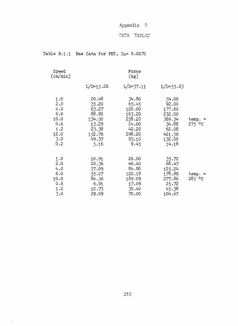
Appendix :3
DATA TABLES
Table B.1.1 Raw Data for PET, De= 0.0270
Speed Force (cm/min) (kg)
L/D=15.26 L/D=37.11 L/D=55,63
i.o 20.48 34.80 54.00 2.0 35,20 65 ,45 92.00 4.0 63.27 120.00 1?7.60 6.o 88.80 163.20 232.00
10.0 134.50 258.~0 369,34 temp. = o.6 13.29 24.00 34.88 275 °c 1.2 23,38 42.20 62.08
12.0 152,76 298.20 421.56 3.0 49,37 93.10 132.00 0.2 5.16 9,45 14.18
i.o 10.91 26.60 35,72 2.0 20.36 46.40 68.47 4.0 37,09 8L~.80 125.24 6.o 55 .27 122.18 178,89 temp. =
10.0 84.J6 1$9,09 277,86 285 °c o.6 6.91 17.09 25.72 1.2 12.73 J0.40 45,38 3.0 29.09 70.00 104.67
210
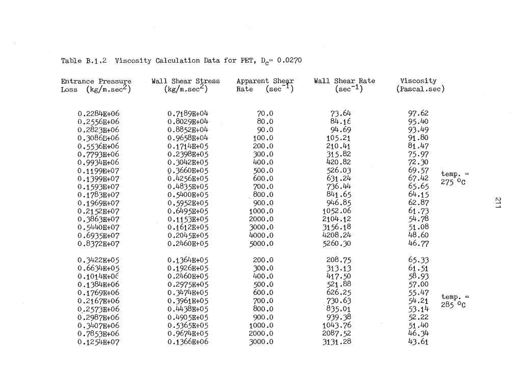
Table B.1.2 Viscosity Calculation Data for PET, De= 0.0270
Entrance Pressure Wall Shear Stress Apparent She~ Wall Shear Rate Viscosity Loss (kg/m.sec2) (kg/m.sec2) Rate (sec- ) (sec-1) (Pascal.sec)
0.2284E+06 o.7189E+04 70.0 73,64 97,62 o.2556E+06 0,8029E+04 80.0 84.16 95,40 0.282JE+06 0.8852E+04 90.0 94.69 93,49 o.3086E+06 0,9658E+04 100.0 105.21 91.80 0,5536E+06 0 .1714E+05 200.0 210.41 81.47 0.7793E+06 0.2J98E+05 300.0 315.82 75,97 0.9934E+06 O.J042E+05 400.0 420.82 72.30 0.1199E+07 Q.J660E+05 500.0 526.03 69.57 temp. = 0 .1J99E+07 0.4256E+05 600.0 631.24 67.42 275 OC 0 .1593E+07 0,48J5E+05 700.0 736.44 65.65 0 .178JE+07 0.5400E+05 800.0 841.65 64.15 0 .1969E+07 0.5952E+05 900.0 946.85 62.87 [\.) __. __. 0 .2152E+07 0.6495E+05 1000.0 1052.06 61.73 0 ,386JE+07 0.1153E+05 2000.0 2104.12 54.78 0 ,5440E+07 0.:t.612E+05 3000.0 3156 .18 51.08 0.6935E+07 0.2045E+05 4000.0 4208.24 48.60 0,8J72E+07 0.2460E+05 5000.0 5260 .JO 46.77
O.J422E+05 0.1J64E+05 200.0 208.75 65,33 0.66J4E+05 0.1926E+05 300.0 313 .13 61.51 0.1014E+OC 0.2460E+05 400.0 417.50 58,93 0 .1384E+06 0.2975E+05 500.0 521.88 57.00 0 .1769E+06 O.J474E+05 600.0 626.25 55,47 temp. = 0.2167E+06 O.J961E+05 700.0 730.63 54.21 0,.2573E+06 o.44J8E+05 800.0 ·835.01 53.14 285 °c 0.2987E+06 0.4905E+05 900.0 939,38 52.22 0 .J407E+06 o.5365E+05 1000.0 1043.76 51.40 0.785JE+06 0.9674E+05 2000.0 2087,52 46,34 0 .1254E+07 0 .1366E+06 3000.0 3131.28 43.61
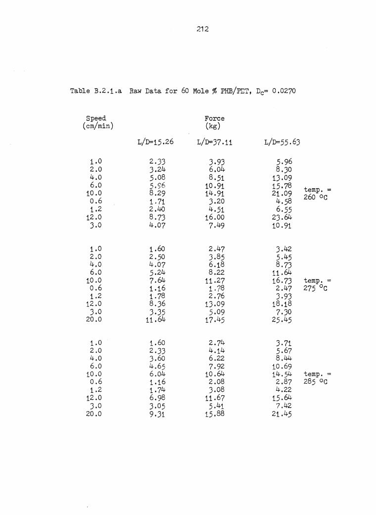
212
Table B.2.1.a Raw Data for 60 Mole% PHB/P£T, De= 0.0270
Speed Force (cm/min) (kg)
L/D=15.26 L/D=37 .11 L/D=55.63
1.0 2.33 3,93 5,96 2.0 3.24 6.04 8.30 4.0 5.08 8.51 13.09 6.o 5 .<;6 10.91 15.78 temp. = 10.0 8.29 14.91 21.09 260 oc o.6 1. 71 3.20 4.58 1.2 2.40 4.51 6.55
12.0 8,73 16.00 23.64 3.0 4.07 7,49 10 .91
1.0 1.60 2.47 3.42 2.0 2.50 3,85 5,45 4.0 4.07 6.18 8,73 6.o 5.24 8.22 11.64
10.0 7,64 11.27 16.73 temp. = 0.6 1.16 1.?8 2.47 275 OC 1.2 1. 78 2.76 3,93
12.0 8.36 13.09 18.18 3.0 3,35 5,09 7.30
20.0 11.64 17.45 25.45
1.0 1.60 2.74 3,71 2.0 2.33 4.14 5,67 4.0 3.60 6.22 8.44 6.0 4.65 7,92 10.69
10.0 6.04 10.64 14.54 temp. = 0.6 1.16 2.08 2.87 285 oc 1.2 1.74 3.08 4.22
12.0 6.98 11.67 15.64 J.O J.05 5.41 7.42
20.0 9.31 15.88 21.45
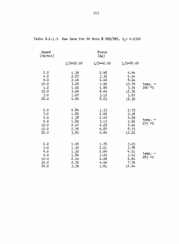
213
Table B.2.1.b Raw Data for 60 Mole% PHB/PET, De= 0.0500
Speed Force (cm/min) (kg)
L/D=20.00 L/D=40.00 L/D=80.00
2.0 1.36 2.48 4.44 4.0 2.07 3.36 6.54 6.0 2.40 4.46 8.44
10.0 3.20 5,90 10.76 temp. = 1.2 1.02 1.84 3,34 260 °c
12.0 3.64 6.64 12.36 3.0 1.67 3.12 5.67
20.0 4.80 8.63 16.36
2.0 0.84 1.53 2.73 3.0 1.82 2.00 3.56 4.0 1.38 2.47 4.29 temp. = 6.0 1.82 3.13 5.60
10.0 2.47 4.29 7.64 275 °c 12.0 2.76 4.87 8.73 20.0 3.85 6.84 12.22
2.0 1.06 1.76 3.05 3.0 1.30 2.21 3,78 4.0 1.52 2.64 4.51 temp. = 6.o 1.84 3.20 5.45
10.0 2.24 4.08 6.84 285 oc 12.0 2.72 4.40 7,76 20.0 3,36 5.81 10.04

214
Table B.2.1.c Raw Data for 60 Mole % PHB/PET, De= 0 .0700
Speed Force (cm/min) (kg)
L/D=14.29 L/D=21.43 L/D=42.86
2.0 0.57 0.75 1.34 4.0 0.88 1.20 2.00 temp. = 6.0 1.13 1.56 2.73
10.0 1.53 2.14 . 3,85 260 oc 12.0 1.78 2.47 4.22 20.0 2.40 3.34 5:82
4.0 0.74 1.02 1. 74 6.0 1.02 1.34 2.33 temp. = 10.0 1.45 1.93 3.42 275 °c 12.0 1.74 2 .18 3,85
20.0 2.33 3.27 5.6o
4.0 0.76 0.97 1.56 6.o 0.94 1.20 2.00 temp. = 10.0 1.17 1.56 2.58
12.0 1.34 1.69 2.87 285 °c 20.0 1.78 2.18 J.64

Table B.2.2.a Viscosity Calculation Data for 6o Mole% PHB/PET, De= 0.0270
Entrance Pressure Wall Shear Stress Apparent Shear Wall Shear Rate Viscosity Loss (kg/m.sec2) (kg/m.sec2) Rate (sec-1) (sec-1) (Pascal.sec)
0. 7847E+05 0.2245E+04 200.0 240.99 9.32 0,9844E+05 0.2805E+04 300.0 361.48 7,76 0 .1156E+06 0.3286E+04 400.0 481.97 6.82 0.1310E+06 0.3714E+04 500.0 602.47 6.11 0 .1451E+06 0.4106E+04 600.0 722.96 5.68 0 .1581E+06 0.4469E+04 700.0 843.45 5,30 temp. = 0 .1704E+06 0.4809E+04 800.0 963,95 4.99 0.1820E+06 0 .5131E+04 900.0 1084.44 4.73 260 °c 0 .1930E+06 0.5436E+04 1000.0 1204.93 4.51 0 . 28Ll4E+06 0.7957E+04 2000.0 2409.87 3.30 0.3567E+06 · 0 . 9942E+04 3000.0 3614.80 2.75 0.4190E+06 0 .1165E+05 4000.0 4819.80 2.42 0 .4747E+06 0.1J16E+05 5000.0 6024.67 2 .19 [\) _.
Vl
0.1024E+06 0.1J81E+04 300.0 335,49 4.12 0.1234E+06 0 .1679E+04 400.0 447.33 3.75 0 .1427E+06 0.1954E+04 500.0 559 .16 3,49 0 .1606E+06 0.2211E+04 6oo.o 670.99 3.30 0.1775E+06 0.2455E+04 700.0 782.82 3.14 0.1936E+06 0.2688E+04 800.0 894.65 3.00 0.2090E+06 0.2911E+04 900.0 1006.48 2.89 temp. = 0.2238E+06 0.3127E+04 1000.0 1118.31 2.80 275 °c 0.3509E+06 0.5006E+04 2000.0 2236.63 2.24 0 .L~566E+06 0.6591E+04 3000.0 3354,94 1.96 0.5503E+06 0.8012E+04 4000.0 4473.26 1.79 0.6360E+06 0.9321E+04 5000.0 5591°57 t.67 0.7159E+06 0 .1055E+05 6000.0 6709.89 1.57 0.7911E+06 0 .1171E+05 7000.0 7828.20 1.50

Table B.2.2.a (Continued)
Entrance Pressure Wall Shear Stress Apparent Shear Wall Shear Rate Viscosity Loss (kg/m.sec2) (kg/m.::;ec2) Rate (sec-1) (sec-1) (Pascal.sec)
0.6751E+05 0.1335E+04 200.0 238,65 5,59 0 .8?16E+05 0 .1678E+o4 300.0 357,97 4.69 0 .1045E+o6 0 .1974E+04 400.0 477,30 4.14 0 .1202E+o6 0.2239E+04 500.0 596.62 3,75 0 .1348E+06 0.2481E+o4 600.0 715.95 3.47 0 .1485E+o6 0.2706E+04 700.0 835.27 3.24 0 .1615E+o6 o· .2918E+04 800.0 954,59 3.06 0 .1739E+06 0.3118E+04 900.0 1073,92 2.90 1.cinp0 = 0.1858E+o6 0.3309E+04 1000.0 1193 .24 2.77 265 c 0 .2868E+o6 0.4891E+04 2000.0 2386.49 2.05 0.3697E+o6 0.6146E+04 3000.0 3579,73 1.72 /\.)
-'
0.4426E+06 0. 7227E+04 4000.0 4772.97 1.51 °' 0.5088E+o6 0.8195E+o4 5000.0 5966.22 1.37 0 .5702E+o6 0 .9081E+04 6000.0 7159.46 1.27 0.6Z78E+06 0.9904E+o4 7000.0 8352.71 1.19 0.6824E+06 0 .t068E+o5 8000.0 95lJ.5 ,95 1.12
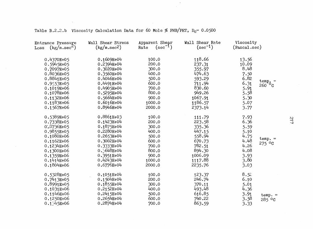
Table B.2.2.b Viscosity Calculation Data for 60 Mole % PHB/PET, De= 0.0500
Entrance Pressure Wall Shear Stress Apparent Sherr Wall Shear Re.te Viscosity Loss (kg/m.sec2) (kg/m.sec2) Rate (sec- ) (sec-1) (Pascal.sec)
0 .4370E+05 0.1609E+04 ioo.o 118.66 13.56 0.5945Et05 0.2394E+04 200.0 237,31 10.09 0.?097E+05 0.3020Et04 300.0 355,97 8.48 0.8036E+05 0.3560E+04 400.0 474.63 7,50 0.8841E+05 0.4046E+04 500.0 593.29 6.82 temp. = 0.955JE+05 0.4491E+04 600.0 711.94 6.31 260 °c 0 .1019E+06 0.4905E+04 700.0 830.6o 5.91 0 .1078E+06 0.5295Et04 800.0 949.26 5,58 0 .1132E+06 0.5664E+04 900.0 1067. 91 5.30 0 .1183E+06 0.60t6E+04 1000.0 1186.57 5.07 0 .1567E+06 0,8946E+04 2000.0 2373.14 3,77
o.5389E+05 0,8861E+03 100.0 111°79 7,93 /\)
0.7338E+05 O.i423E+04 200.0 223.58 6.36 ....... --..]
o:~8736E+05 o.1875E+04 300.0 335,36 5,59 0.9855E+05 0.2280Et04 400.0 447.15 5.10 0.1080E+06 0.2653Et04 500.0 558,94 4.75 temp. = 0 .1162E+06 0.3002Et04 600.0 670.73 4.48 0.1234E+06 0.3333E+04 700.0 782.51 4.26 275 °c 0 .1300Et06 o • .:;.648E+04 800.0 894,30 4.08 0.1359E+06 0.3951Et04 900.0 1006.09 3,93 0 .1414E+06 0.4243E+04 1000.0 1117.88 3.80 0 .1804E+06 o.6776m+o4 2000.0 2235,76 3.03
0,5328E+05 0.1051E+04 100.0 123,37 8.52 0.7413E+05 0 .1504E+04 200.0 246.74 6.10 0.8991E+05 o.1855m+o4 300.0 370.11 5.01 0.1031E+06 0.2152E+04 400.0 493.48 4.36 0.1146E+06 0.2415E+04 500.0 616.85 3.91 temp. = 0 .1250E+06 0.2654E+04 6oo.o 740.22 3,58 285 °c O • C·l~5E+06 0.2874E+04 700.0 863.59 3,33
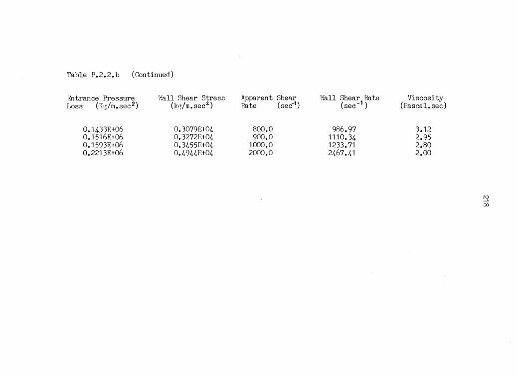
Tahle B.2.2. b (Continued)
Entrance Pressure Loss (K~/m.sec2)
0.1433E+06 0.1516E+06 0.1593E+06 0.22131~+06
\•!all Shear Stress (h;/m.sec2.)
O. 3079F~+04 0.3272E+04 0.3455E+04 0.4944E+04
Apparent Shear Rate (sec1)
800.0 900.0
1000.0 2000.0
1,<fall Shear Hate (sec-1 )
986.97 1110.34 1233.71 2467.41
Viscosity (Pascal. se~)
3.12 2.95 2.80 2.00

Ta~;le B.2 .2 .c Viscosity Calculation Data for 60 Mole % PHB/PET, De= 0.0700
Entrance Pressu2e Wall Shear Stress Apparent Shear Wall Shear Rate Viscosity Loss (kg/m.sec ) (kg/m.sec2) Rate {sec-1) {sec-1) {Pascal.sec)
0.2534E+05 0.8648E+03 40.0 45.20 19.13 0.2887E+05 0.1002E+04 50.0 56.50 17.73 0.3210E+05 0.UJOE+04 60.0 67.80 16.66 0.3512E+05 0.1250E+04 70.0 79.10 15.81 0.3796E+05 0.1J65E+04 80.0 90.40 15.10 temp. = 0 .Ll-065E+05 0.1475E+04 90.0 101. 70 14.51 0.4322E+05 0 .1581E+04 100.0 113.00 13.99
26o OC 0.6464E+05 0.2495E+04 200.0 226.00 11.04 0.8174E+05 0.3258E+04 300.0 339.01 9.61 0.9652E+05 0.3937E+04 400.0 452.01 8.71 0 .1098E+06 0.456oE+04 500.0 565.01 8.07
/\.) -"
0.3459E+05 0.1122E+04 80.0 87.27 12.85 -..o 0.3751E+05 0 .1223E+04 90.0 98.17 12.46 o.4034E+05 0.1J21E+04 100.0 109.08 . 12 .11 temp. = o.6504E+05 0.2197E+04 200.0 218 .16 10.07 275 OC 0.8597E+05 0.2958E+04 300.0 327.24 9.04 o.1048E+06 0.3653E+04 400.0 436.33 8,37 0.1222E+06 0.4J03E+04 500.0 545.41 7.89
0.4555E+05 0.9610E+03 80.0 97.30 9,88 0.4821E+05 0.1024E+04 90.0 109.46 9,35 0.5071E+05 O .1083E+04 100.0 121.62 8.91 temp. = 0. 7078E+05 0 .1571E+04 200.0 243.24 6.46 285 OQ 0.8599E+05 0 .1953E+04 300.0 364.86 5,35 0.9872E+05 0.2279E+04 400.0 486.48 4.68 0.1099E+06 0.2569E+04 500.0 608.10 4.22
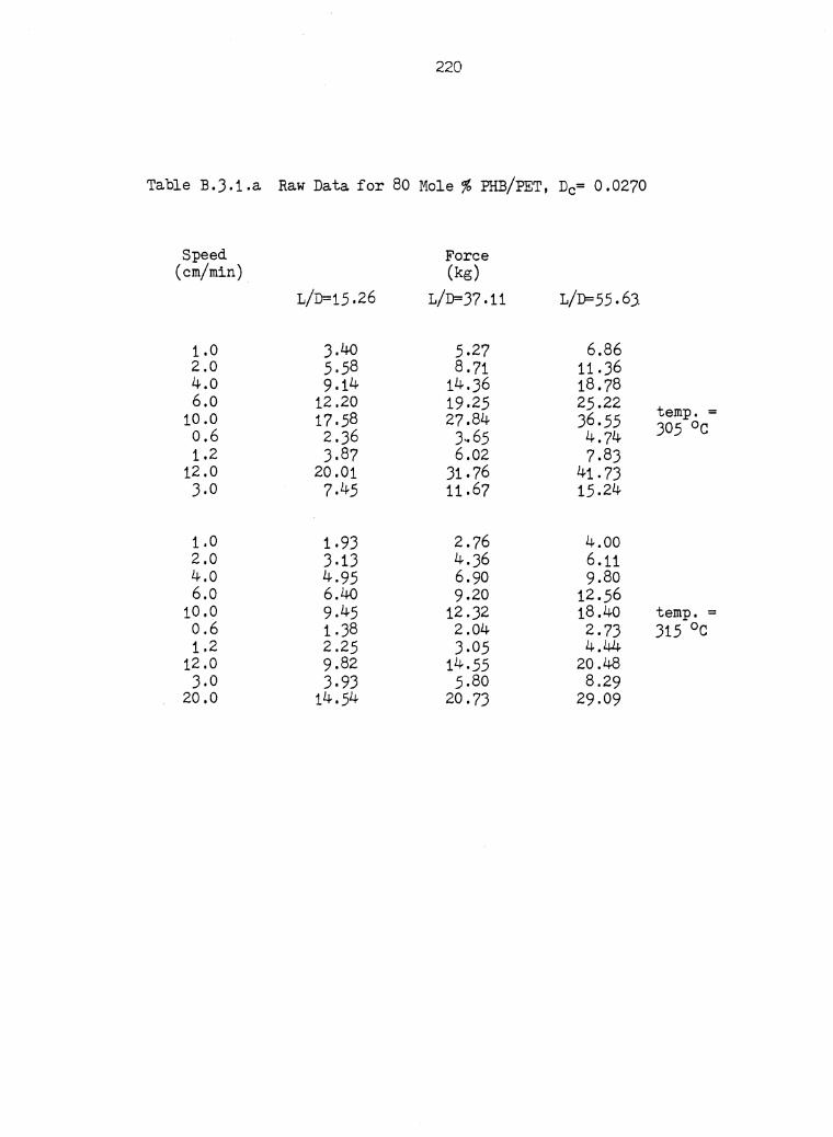
220
Table B.3.1.a Raw Data for 80 Mole% PHB/PET, De= 0.0270
Speed Force (cm/min) (kg)
L/D=15.26 L/D=37.11 L/D=55.63.
1.0 3.40 5,27 6.86 2.0 5,58 8.71 11.36 4.0 9 .14 14.36 18.78 6.0 12.20 19.25 25.22 temp. = 10.0 17.58 27.84 36.55 0.6 2.36 3~65 4.74 305 °c 1.2 3,87 6.02 7,83
12.0 20.01 31.76 41.73 3.0 7,45 11.67 15.24
1.0 1.93 2.76 4.00 2.0 3,13 4.36 6.11 4.0 4.95 6.90 9.80 6.o 6.40 9.20 12.56
10.0 9,45 12.32 18.40 temp. = 0.6 1.38 2.04 2.73 315 °c 1.2 2.25 3.05 4.44
12.0 9.82 14.55 20.48 3.0 3,93 5.80 8.29
20.0 14.54 20.73 29.09

221
Table B.3.1.b Raw Data for 80 Mole% PHB/PET, De= 0.0500
Speed Force (cm/min) (kg)
L/D=20. L/D=40. L/D=80.
1.0 1.10 1.53 2.51 2.0 1.75 2.55 3.93 4.0 2.69 3.78 6.11 6.0 3.64 5.16 8.65 temp. = 10.0 4.94 7.13 11.64 1.2 1.27 1.78 2.87 305 °c
12.0 5.82 8.36 1J.82 3.0 2.40 3.27 5.09
20.0 8.00 11.64 18.18
1.0 0.75 1.02 1.71 2.0 1.14 1.60 2.58 4.0 1.80 2.54 3,93 6.o 2.33 3.34 5.45 temp. = 10.0 3.20 4.58 6.91 315 °c 1.2 0.88 1.24 1.93
12.0 3.56 4.94 8.00 3.0 1.60 2.11 3.42
20.0 4.87 7,05 10.84
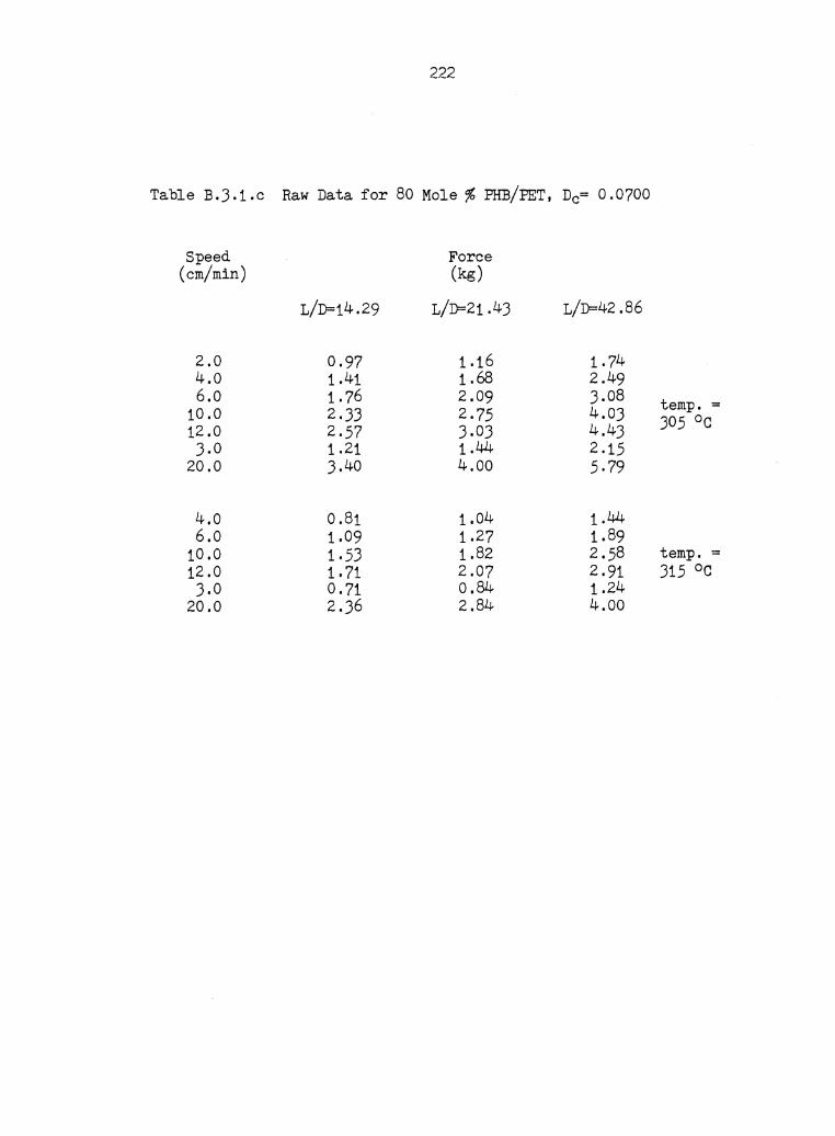
222
Table B.3.1.c Raw Data for 80 Mole% PHB/PET, De= 0.0700
Speed Force (cm/min) (kg)
L/D=14.29 L/D=21.43 L/D=42.86
2.0 0.97 1.16 1.74 4.0 1.41 1.68 2.49 6.0 1.76 2.09 3.08 temp. = 10.0 2.33 2.75 4.03 305 °c 12.0 2.57 3.03 4.43 3.0 1.21 1.44 2 .15
20.0 3.40 4.00 5,79
4.0 0.81 1.04 1.44 6.0 1.09 1.27 1.89
10.0 1.53 1.82 2.58 temp. = 12.0 1.71 2.07 2.91 315 °c 3.0 0.71 o.84 1.24
20.0 2.36 2.84 4.00

Table B.3.2.a Viscosity Calculation Data for 80 Mole% PHB/PET, De= 0.0270
Entrance Pressure Wall Shear Stress Apparent Shear Wall Shear Rate Viscosity Loss (kg/m.sec2) (kg/m.sec2) Rate {sec-1) {sec-1) (Pascal.sec)
0.2460E+06 0.2501E+04 300.0 326.50 7.66 0.3007E+06 0.3093E+04 400.0 435.33 7 .10 0.3513E+06 0.3647E+04 500.0 544.16 6.70 0.3990E+06 0.41)7E+04 600.0 653.00 6.39 0.4442E+06 0.4677E+04 700.0 '761.83 6.14 temp. = 0.8476E+06 0.5161E+04 800.0 870.66 5.93 305 °c 0. 52c1lE+06 0.5631E+04 900.0 1088.31 5,59 o. 5r;96~~+06 0 .6o86E+04 1000.0 10RR,33 5.59 0.9233E+06 0 .1016E+05 2000.0 2176.66 4.67 0.1255E+07 0 .1370E+05 3000.0 3264.98 4.20 0 .1496E+07 0 .1694E+05 4000.0 4353.31 3.89 0 .1748E+07 0 .1998E+05 5000.0 5441.64 3.67 N
/\) 'vJ
0.1355E+06 0 .1469E+04 300.0 336.91 4.36 0 .1640E+06 0 .178tE+04 400.0 449.21 3,97 0 .1902E+06 0.2068E+04 500.0 561.51 3.68 0.2146E+06 0.2337E+04 600.0 673.81 3.47 0.2377E+06 0.2592E+04 700.0 786 .12 3.30 temp. = 0.2598E+06 0.2834E+04 800.0 898.42 3.15 315 OC 0.2809E+06 0.3067E+04 900.0 1010.72 3.03 0.3012E+06 0.3292E+04 1000.0 1123.02 2.93 0.4772E+06 0,5238E+04 2000.0 2246.05 2.33 0.6245E+06 0.6873E+04 3000.0 3369.07 2.04 0.7558E+06 0,8JJ5E+04 4000.0 4492.09 1.86 0.8765E+06 0.9679E+04 5000.0 5615.11 1.72 0.9892E+06 0 .1094E+05 6000.0 6738 .14 1.62 0 .1096E+07 0 .1213E+05 7000.0 7861.16 1.54

Table B.J.2.b Viscosity Calculation Data for 80 Mole% PHB/PET, Dc=0.0500
Entrance Pressure Wall Shear Stress Apparent Shear Wall Shear Rate Viscosity Loss (kg/m.sec2) (kg/m.sec2) Rate (sec-1) (sec-1) (Pascal.sec)
0.7982E+05 0.7094E+03 50.0 55,85 12.70 0.8976E+05 0.80J2E+03 60.0 67.02 11.98 0.9913E+05 0.8922E+03 70.0 78.20 11.41 0 .1080E+06 0.9772E+03 80.0 89,37 10.93 0.1165E+06 0.1059E+04 90.0 100.54 10.53 0 .1247E+06 0 .1138E+04 100.0 111. 71 10.18 0 .1948E+06 0.1824E+04 200.0 223.42 8 .17 0.2528E+06 0.2405E+04 300.0 335 .12 7 .18 temp. = 0 .3042E+06 0.2925E+04 400.0 446.83 6.55 305 °c 0 .3511E+06 0.3405E+04 500.0 558,54 6.10 O.J948E+06 O.J855E+04 600.0 670.25 5,75 0.4359E+06 0.4282E+04 700.0 781.96 5.48 j\)
0.4750E+06 0.4690E+04 800.0 893.67 5.25 N ~
0.512JE+06 0 .5081E+o4 900.0 1005.37 5,05 0.5482E+o6 0 .5459E+o4 1000.0 1117.08 4.89 0.8557E+06 0.8751E+04 2000.0 2234.16 3,92
0.5429E+05 0.4946E+OJ 50.0 58.00 8,53 0.6099E+05 0.5528E+03 60.0 69.60 7,94 0.6730E+05 0.607JE+03 70.0 81.20 7,48 0 .7J29E+05 0.6589E+03 80.0 92.80 7.10 0.7901E+o5 0.7080E+OJ 90.0 104.40 6.78 0.8451E+05 0.7550E+oJ 100.0 116.00 6.51 0.1J15E+ot 0 .1152E+04 200.0 231.99 4.97 0 .1704E+06 0 .1475E+04 JOO.O 347.99 4.24 temp. = 0.2047E+ot 0 .1758E+04 400.0 463,99 3,79 315 °c 0 .2J60E+06 0.2015E+04 500.0 579,99 3,47 0.2651E+o6 0.2252E+04 600.0 695.98 J.24 0.2926E+o6 0.2474E+o4 700.0 811.98 3.05

Table R.3.2.b (Continued)
Entrance Pressure Loss (I\c;/rn.sec2 )
0.3186E+06 0.3434E+06 0.3673F.+06 0.5715E+06
\fall Shear Stress (Kg/rn.sec2 )
0.2683E+04 0.2883E+04 0.3074E+04 0.4691E+04
Apparent Shear Rate (sec-')
800.0 900.0
1000.0 2000.0
\·rall Shear Rate (sec- 1 )
927.98 1043. 98 1159.97 2319.95
Viscosity (Pascal.sec)
2.89 2.76 2.65 2.02
/\) /\) \J'l
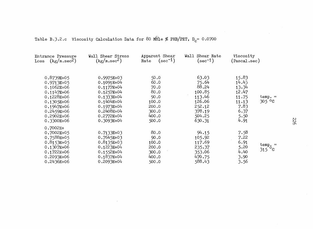
Table B.3.2.c Viscosity Calculation Data for 80 M8le % PHB/PET, De= 0.0700
Entrance Pressure Wall Shear Stress Apparent Shear Wall Shear Rate Viscosity Loss (kg/m.sec2) (kg/m.sec2) Rate (sec-1) (sec-1) (Pascal.sec)
0.8739E+05 0.9975E+03 50.0 63.03 15.83 0.9713E+05 0 .1091E+04 6o .o 75.64 14.43 0 .1062E+06 0 .1177E+04 70.0 88.24 13.34 0 .1147E+06 0 .1257E+04 80.0 100.85 12.47 0 .1228E+06 0 .1333E+04 90.0 113 .46 11.75 temp. = 0 .1J05E+06 0 .1404E+04 100.0 126 .06 11.13 305 °c 0 .1947E+06 0 .1973E+OLJ. 200.0 252 .12 7,83 0.2459E+06 0.2408E+04 300.0 378 .19 6,37 0.2902E+06 0.2772E+04 400.0 504.25 5.50 0.3300E+06 0.3093E+04 500.0 630.31 4.91 /\)
/\)
°" 0.7002E+ 0.7002E+05 0.71J3E+03 80.0 94.15 7.58 0.7588E+05 o.7645Frt03 90.0 105.92 7.22 0.8153E+05 0 ,81J5E+03 100.0 117.69 6.91 temp. = 0 .1307E+06 0.1223E+04 200.0 235,37 5.20 315 °c 0 .1722E+06 0 .1552E+04 300.0 353.06 4.40 0.2093E+06 0.1837E+04 400.0 470.75 3.90 0.2436E+06 0.2093E+04 500.0 588.43 3.56
Appendix C
NOMENCLATURE
A Cross Sectional Area of Plunger (m 2 )
B Cavity Thickness
Db Diameter of Barrell (m)
Dj Diameter of Extrudate (m)
de Diameter of Capillary (m)
dp Diameter of Plunger (m)
K Rate of Elongation
L Length of Capillary (m)
M Entrance Length Correction (Dimensionless)
N~ First Normal Stress Difference (Kg/m.secz)
n Power-Law Index
P Pressure (Kg/m.sec2)
Q Flow Rate (cm /sec)
R Radius (m)
S Molecular Order Parameter (Dimensionless)
S Plunger Speed (m/sec)
Sr Recoverable Shear Strain
T Temperature (°K)
T~ Glass Transition Temperature (°K)
Tm Melt Temperature (°K)
Vi Velocity in i direction (m/sec)
(V) Average Velocity (m/sec)
227

228
iAPP Apparent Shear Rate (l/sec)
~W Wall Shear Rate (1/sec)
APeri Entrance Pressure Loss (Kg/rn.sec 2 )
~ Melt Viscosity (Pascal.Sec)
n• ., Complex Viscosity (Pascal.Sec)
Yl~ Viscosity at Core (Pascal.Sec)
V'l.w Viscosity at Wall (Pascal.Sec)
~ Apparent Viscosity (Pascal.Sec) ' \Af P p Density (Kg/rn3)

The vita has been removed from the scanned document
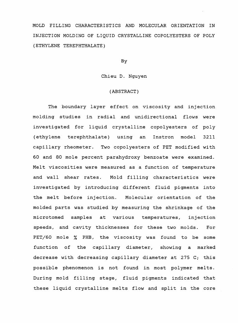
MOLD FILLING CHARACTERISTICS AND MOLECULAR ORIENTATION IN
INJECTION MOLDING OF LIQUID CRYSTALLINE COPOLYESTERS OF POLY
(ETHYLENE TEREPHTHALATE)
By
Chieu D. Nguyen
(ABSTRACT)
The boundary layer effect on viscosity and injection
molding studies in radial and unidirectional flows were
investigated for liquid crystalline
(ethylene terephthalate) using an
copolyesters of poly
Instron model 3211
capillary rheometer. Two copolyesters of PET modified with
60 and 80 mole percent parahydroxy benzoate were examined.
Melt viscosities were measured as a function of temperature
and wall shear rates. Mold filling characteristics were
investigated by introducing different fluid pigments into
the melt before injection. Molecular orientation of the
molded parts was studied by measuring the shrinkage of the
microtomed samples
speeds, and cavity
at various temperatures, injection
thicknesses for these two molds. For
PET/60 mole % PHB, the viscosity was found to be some
funct~on of the capillary diameter, showing a marked
decrease with decreasing capillary diameter at 275 C; this
possible phenomenon is not found in most polymer melts.
During mold filling stage, fluid pigments indicated that
these liquid crystalline melts flow and split in the core

before they approach the flow front. Molecular orientation
studies showed that high shrinkage across the flow direction
than that measured along the flow direction. Studies also
indicated that there existed a relative maximum molecular
orientation away from the surf ace of the parts,
corresponding to the shear zone. As the cavity thickness
decreases or injection speed increases, this relative
maximum peak moves to the surface of the molded parts.