1

Forecasting Price Relationships among U.S Tree Nuts Prices

Mohammed Ibrahim

Fort Valley State University 1005 State University Dr.

Fort Valley, GA 31030 Tel: (478) 825-6815

E-mail: ibrahimm@fvsu.edu

Wojciech J. Florkowski

Department of Agricultural and Applied Economics The University of Georgia, Griffin E-mail: wflorko@griffin.uga.edu

Paper Prepared for Presentation at the Southern Agricultural Economics

Association Annual Meeting, Atlanta, Georgia, January 31-February 3, 2009

Copyright 2009 by M. Ibrahim and W.J. Florkowski. All rights reserved. Readers may make verbatim copies of this document for non-commercial purposes by any means, provided that this copyright notice appears on all such copies.

2

Forecasting Price Relationships among U.S Tree Nuts Prices

Abstract

This paper investigates a vector auto regression model, using the Johansen cointegration technique, and the autoregressive integrated moving average time series models to determine the better model for forecasting US tree nut prices over the period 1992-2006. The Johansen contegration test shows lack of long run relationship among pecan, walnut, and almond prices. As such, only autoregressive integrated moving average-type models were used in forecasting U.S. nut prices. Keywords: substitutability, cointegration, tree nuts, long-run equilibrium forecasting.

3

Introduction

The U.S. is not only the world’s leading producer, but also the leading exporter of

tree nuts (Johnson, 1998). Tree nuts remain an important component of the American

diet. The growth in demand for tree nuts may be attributed to the increase in knowledge

of the health benefits of nuts, an increase in per capita income and the increase in

introductions of new products by a rapidly expanding bakery and confectionery industry.

U.S. tree nuts (henceforth referred to as ‘nuts’) are used in snacks, breakfast cereal, ice

cream, and confections (Lin et al., 2001). The U.S. tree nut industry is a multibillion

industry (USDA, 2003). Some of the most popular tree nuts are almonds, pecans, and

walnuts. Although all kinds of nuts have very specific and different uses, some

substitutability does occur between and among the nuts (Florkowski and Lai, 1997). For

example, walnuts or almonds cannot be substituted for pecans in a pecan pie, but this can

happen in a breakfast cereal or a nut mix snack.

As a consequence, a better understanding of the relationships among tree nut

prices is crucial for the tree nut industry. The results of this study contribute to the

exploration of the market structure, product substitutability, competitiveness of nut

markets and price forecasts.

To our knowledge, there are no empirical studies dealing with forecasting price

relationships among U.S. tree nut prices. Earlier studies, however, provide examples of

how the cointegration technique is useful in the forecasting process (Florkowski and Lai,

1997; Lanza et al., 2005). In the context of nut prices, Florkowski and Lai (1997) studied

the relationship between pecan and other edible nut prices using the cointegraton

4

technique. The study found a cointegration between prices of pecans and almonds and

pecans and walnuts. The results were used to improve price forecasts. The study used

processor prices of two grades of each kind of nut.

The objective of this paper is to forecast cointegrated relationships among

selected U.S. tree nut prices employing the Johansen and Juselius (1990) maximum

likelihood procedure. For the purpose of comparison, an autoregressive integrated

moving average, first introduced by Box and Jenkins (1976), is used in forecasting the

univariate variables.

The Johansen Cointegration Procedure

Engle and Granger (1987) argue in the seminal paper that differencing used to

make data stationary in the traditional Box and Jenkins type models causes the loss of

information on the long run effects. The cointegration technique, which accommodates

deviations from the equilibrium condition for two or more economic variables that are

nonstationary when taken by themselves, was developed by Engle and Granger (1987) to

address this problem. Since then, economists have extended and also applied the

cointegration technique to wide ranging sets of economic data (Johansen, 1988; Johansen

and Juselius, 1990; Luppold and Prestemon, 2003). In this study, the Johansen type of the

contegration technique is used because it is more powerful than the Engle and Granger

procedure (MacDonald and Taylor, 1994). Following Johansen and Juselius (1990), the

error correction model can be written as

(1) tttit

p

i

it ADXXX ε++Π+∆Φ=∆ −−

−

−

∑ 1

1

1

where iΦ = ( )iI Γ+Γ+− ,...,1

5

and Π = ( )pI Γ−−Γ−− ,...,1 .

Other terms in (1) include: tε are the error terms and are drawn from a p-dimensional

i.i.d. normal distribution with covariance Λ ; tD is a deterministic term, which may

contain a constant, a linear trend or seasonal dummy variables, or both. The impact

matrix,Π , determines whether or not there are significant long-run relationships among

variables in the system. If the rank of Π matrix r is pr <<0 , then there are two matrices

α and β each with dimension p x r such that Π=′βα , while r is the number of

cointegrating relationships among variables in tX . The matrix β of r cointegrating

vectors consists of elements of tXβ ′ that are stationary. The matrix of error correction

parameters α measures the speed of adjustment in tX∆ .

In order to use the cointegration technique in the forecasting process, the series

must be cointegrated. Johansen (1988) proposes the following trace test statistic:

(2) ( ) ( )∑+=

−−=n

tj

jtrace Tr1

ˆ1log λλ

where T is the number of observations in the data. The trace test has its null hypothesis

that there are at most r cointegrating vectors. The alternative hypothesis states that there

are more than r cointegrating vectors in the system. The trace test has a non-standard

distribution (Johansen and Juselius, 1990). The series are cointegrated if r is not equal to

zero and there are r cointegrated relationships among the series, and the error correction

method is appropriate for the data.

Univariate Time Series

The more popular autoregressive integrated moving average (ARIMA) method is

applied in the case of the univariate time series. The ARIMA procedure (Box and

6

Jenkins-type model) generally involves four steps; identification, model estimation,

diagnostics and forecasting. The technique assumes that the time series under

consideration is stationary. Therefore, the first step in estimating an ARIMA model is to

test for stationarity. If the series is not stationary then transformation or differencing is

needed to make the time series stationary. The differencing of non-stationary series,

however, results in a significant loss of information on long run trends (Engle and

Granger, 1987).

The general form of the ARIMA model is written as ARIMA (p,d,q), where the p

represents the autoregressive part of the model, d is the order of differencing to make the

series stationary, and q represents the moving average part of the model. Algebraically,

the general ARIMA ( p,d,q) model is written as:

( )( ) ( ) tqt

d

p LZLL αθθφ +=− 01

( )Lpφ represents AR part: p

pLL φφ −−− ...1

( )Lqθ represents MA part: q

qLL θθ −−− ...1 1

tα represents a zero mean white noise process with constant variance.

Data

Monthly prices of the U.S. shelled tree nut grades were obtained from USDA for

the period beginning in January1992 through May 2006. The data include pecan “fancy

halves”, walnuts “light halves and pieces”, and almonds “nonpareil supreme” prices. We

chose to analyze the three price series because of the paucity of data for other kinds of

tree nuts or because other domestically produced tree nuts (e.g., pistachios) are sold

mostly as an in-shell product. Moreover, the chosen nuts appear to be the three most

7

popular among the U.S. consumers. All data refer to the shelled basis, nominal and

wholesale prices (free on board-FOB) from a location in the southeastern U. S.

Table 1 shows the summary statistics for the nut price series. The statistics refer

to the high end grades of the three kinds of nuts and the mean prices reflect the overall

availability of each nut and the domestic demand. Pecans were traded at a premium to

both walnuts and almonds with mean prices $1.41 and $1.26 per pound higher,

respectively. Pecan prices also showed the widest range between the minimum and the

maximum price, which likely results from the tendency to pecan trees to bear in alternate

years. Walnuts, on the other hand, sold at a premium to almonds with a mean price of

$0.15 per pound higher. However, almond prices showed the highest variability and the

largest standard deviation among the three kinds of nuts considered in this study.

Figure 1 shows the plots of price series for pecans, almonds and walnuts between

January 1992 and May 2006. During the period under consideration, the prices of pecans

and walnuts were generally higher than those of almonds except in 1996 and 1997. In

these two years the prices of pecans were lower than those of almonds or walnuts, while

almond prices were on par or higher than walnut prices reaching the highest level

between 1992 and 2002. Since 1997, the prices of three nut types returned to the pattern

observed in the early 1990s.

Results

The first step in applying the cointegration technique is to test for stationarity. The

results of the stationarity test are summarized in Table 2. All price series were found to

be nonstationary. The trace statistic was used to test for cointegration. Table 3 shows

results of the Johansen’s test. The series are shown not to be cointegrated. Since the

8

condition cointegration is not met the VECM model is not applicable. The results imply

that there is no long run relationship among the substitutes. The findings are inconsistent

with earlier conclusions by Florkowski and Lai (1997).

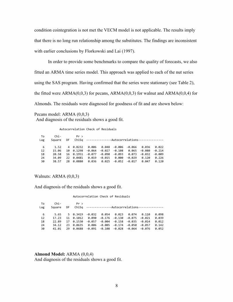
In order to provide some benchmarks to compare the quality of forecasts, we also

fitted an ARMA time series model. This approach was applied to each of the nut series

using the SAS program. Having confirmed that the series were stationary (see Table 2),

the fitted were ARMA(0,0,3) for pecans, ARMA(0,0,3) for walnut and ARMA(0,0,4) for

Almonds. The residuals were diagnosed for goodness of fit and are shown below:

Pecans model: ARMA (0,0,3) And diagnosis of the residuals shows a good fit.

Autocorrelation Check of Residuals

To Chi- Pr >

Lag Square DF ChiSq ---------------Autocorrelations---------------

6 1.52 4 0.8232 0.006 0.048 -0.006 -0.066 0.036 0.022

12 15.06 10 0.1298 -0.064 -0.027 -0.108 0.065 -0.080 -0.214

18 20.58 16 0.1951 -0.077 -0.090 -0.093 0.073 -0.032 -0.009

24 34.09 22 0.0481 0.019 -0.015 0.000 -0.029 0.120 0.226

30 38.57 28 0.0880 0.036 0.025 -0.052 -0.017 0.047 0.120

Walnuts: ARMA (0,0,3)

And diagnosis of the residuals shows a good fit.

Autocorrelation Check of Residuals

To Chi- Pr >

Lag Square DF ChiSq ---------------Autocorrelations---------------

6 5.65 5 0.3419 -0.032 0.054 0.023 0.074 0.110 0.098

12 17.23 11 0.1012 0.090 -0.176 -0.130 -0.075 -0.021 0.039

18 22.89 17 0.1530 -0.057 -0.004 -0.158 -0.035 -0.014 0.012

24 34.12 23 0.0635 0.006 -0.005 -0.174 -0.050 -0.057 0.142

30 41.01 29 0.0688 -0.091 -0.108 -0.028 -0.064 -0.076 0.052

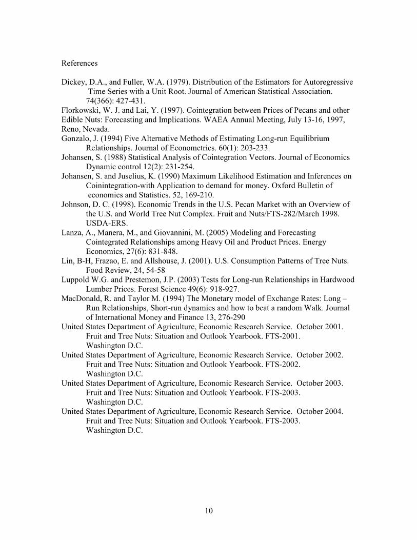
Almond Model: ARMA (0,0,4) And diagnosis of the residuals shows a good fit.

9

Autocorrelation Check of Residuals

To Chi- Pr >

Lag Square DF ChiSq ---------------Autocorrelations---------------

6 3.25 5 0.6619 0.102 0.075 -0.023 -0.018 -0.005 0.039

12 13.87 11 0.2401 -0.004 -0.104 -0.174 -0.071 -0.104 0.030

18 17.42 17 0.4262 -0.054 -0.030 -0.054 -0.055 -0.000 0.093

24 22.84 23 0.4701 0.133 0.048 0.067 -0.010 0.026 -0.046

30 27.60 29 0.5393 0.117 0.015 -0.033 -0.089 -0.005 -0.014

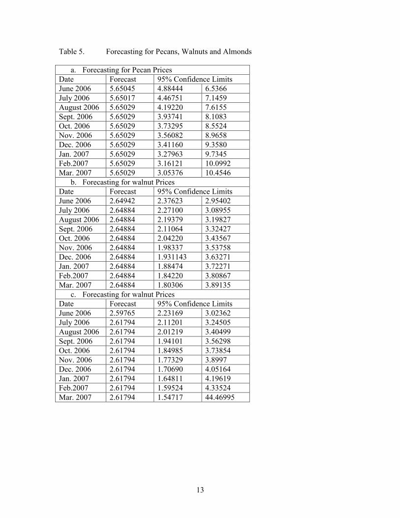
Forecasting

The intention of this paper was to find a better forecasting model between ARIMA and

VEC models. But only ARMA models were used because the cointegration test showed

lack of long run relationships among the nut prices, a prerequisite for using VECM to

make forecasts. The estimated ARMA models outlined above were used to generate

forecasts for monthly nut prices for the period June 2006 to march 2007. The forecasts

are listed in Table 5.

Concluding Remarks

The result of no cointegration among the U.S. tree nuts was disappointing.

Because, we think, there is usually some substitutability among nuts, we expect a

relationship among those nut prices to exist. One possible answer to the lack of

relationship is the data used in the study. Secondary data were used and the quality of the

data is not known. We therefore conclude that, by default, the ARIMA-type models are

better at forecasting U.S. nut prices. However, further examining of the data and re-

constructing the VECM, to allow direct forecast performance comparison, is an important

subject for further research.

10

References Dickey, D.A., and Fuller, W.A. (1979). Distribution of the Estimators for Autoregressive

Time Series with a Unit Root. Journal of American Statistical Association. 74(366): 427-431.

Florkowski, W. J. and Lai, Y. (1997). Cointegration between Prices of Pecans and other Edible Nuts: Forecasting and Implications. WAEA Annual Meeting, July 13-16, 1997, Reno, Nevada. Gonzalo, J. (1994) Five Alternative Methods of Estimating Long-run Equilibrium

Relationships. Journal of Econometrics. 60(1): 203-233. Johansen, S. (1988) Statistical Analysis of Cointegration Vectors. Journal of Economics

Dynamic control 12(2): 231-254. Johansen, S. and Juselius, K. (1990) Maximum Likelihood Estimation and Inferences on

Coinintegration-with Application to demand for money. Oxford Bulletin of economics and Statistics. 52, 169-210.

Johnson, D. C. (1998). Economic Trends in the U.S. Pecan Market with an Overview of the U.S. and World Tree Nut Complex. Fruit and Nuts/FTS-282/March 1998. USDA-ERS.

Lanza, A., Manera, M., and Giovannini, M. (2005) Modeling and Forecasting Cointegrated Relationships among Heavy Oil and Product Prices. Energy Economics, 27(6): 831-848.

Lin, B-H, Frazao, E. and Allshouse, J. (2001). U.S. Consumption Patterns of Tree Nuts. Food Review, 24, 54-58

Luppold W.G. and Prestemon, J.P. (2003) Tests for Long-run Relationships in Hardwood Lumber Prices. Forest Science 49(6): 918-927.

MacDonald, R. and Taylor M. (1994) The Monetary model of Exchange Rates: Long – Run Relationships, Short-run dynamics and how to beat a random Walk. Journal of International Money and Finance 13, 276-290 United States Department of Agriculture, Economic Research Service. October 2001.

Fruit and Tree Nuts: Situation and Outlook Yearbook. FTS-2001. Washington D.C.

United States Department of Agriculture, Economic Research Service. October 2002. Fruit and Tree Nuts: Situation and Outlook Yearbook. FTS-2002. Washington D.C.

United States Department of Agriculture, Economic Research Service. October 2003. Fruit and Tree Nuts: Situation and Outlook Yearbook. FTS-2003. Washington D.C.

United States Department of Agriculture, Economic Research Service. October 2004. Fruit and Tree Nuts: Situation and Outlook Yearbook. FTS-2003. Washington D.C.

11

Table 1. Summary of Selected Tree Nut Prices in the U.S.

Nut price Mean ($/lb)

Standard deviation

Coefficient of variation

Minimum ($/lb)

Maximum ($/lb)

Pecan 3.67 0.94 25.50 2.03 5.80

Almond 2.21 0.71 32.02 1.23 4.25

Walnut 2.26 0.39 17.03 1.58 3.05

Table 2. Results of the Dickey Fuller Unit Root Test on Selected Price Series.

a. DF test for Transformed U.S .Tree Nut Prices Before First Order Difference

Variable Type Rho Pr<Rho Tau Pr<Tau

Pecans Zero Mean -0.09 0.6608 -0.09 0.6519

Single Mean -12.79 0.0643 -2.33 0.1634

Trend -15.56 0.1548 -2.69 0.2441

Walnuts Zero Mean -0.07 0.6971 -0.07 0.7054

Single Mean -10.17 0.1243 -2.29 0.1773

Trend -10.16 0.4141 -2.28 0.4430

Almonds Zero Mean -0.41 0.5881 0.29 0.5791

Single Mean -7.26 0.2539 -1.88 0.3432

Trend -7.55 0.6123 -1.91 0.6448

b. DF test for Transformed US Tree Nut Prices After First Order Difference

Variable Type Rho Pr<Rho Tau Pr<Tau

Pecans Zero Mean -121.90 0.0001 -7.76 <.0001

Single Mean -122.25 0.0001 -7.75 <.0001

Trend -123.20 0.0001 -7.75 <.0001

Walnuts Zero Mean -150.90 0.0001 -8.64 <.0001

Single Mean -151.68 0.0001 -8.63 <.0001

Trend -151.74 0.0001 -8.61 <.0001

Almonds Zero Mean -128.79 0.0001 -8.00 <.0001

Single Mean -129.27 0.0001 -7.99 <.0001

Trend -129.26 0.0001 -7.96 <.0001

12

Table 3. Cointegration Rank Test for Transformed U.S. Tree Nut Prices

The Johansen Rank using trace test

H0: H1: Eigenvalue Trace statistic

5% Critical value Rank=r Rank>r

0 0 0.0608 16.3674 24.08

1 1 0.0313 5.5736 12.21

2 2 0.0006 0.1013 4.14

Table 4. Model Diagnostics for Transformed U.S. Tree Nut Prices

a. Univariate Model ANOVA Diagnostics

Variable R-square Standard deviation F value Pr>F

Pecan - 0.07722 - -

Walnut 0.0568 0.05464 5.09 0.0098

Almond 0.0082 0.07768 0.70 0.4966

C. Univariate Model White Noise Diagnostics

Variable Durbin Watson

Normality ARCH

Chi Sq Pr>Ch sq F value Pr > F

Pecan 1.48784 560.20 <0.0001 1.46 0.2294

Walnut 2.00434 127.99 <0.0001 10.20 0.0017

Almond 1.82001 513.90 <0.0001 0.07 0.7923

C. Univariate Model AR Diagnostics

Variable AR1 AR2 AR3 AR4

F value

Pr>F F value Pr>F F value Pr>F F value

Pr>F

Pecan 11.86 0.0007 5.88 0.0034 4.40 0.0053 3.97 0.0042

Walnut 0.00 0.9760 0.40 0.6731 2.43 0.0668 2.19 0.0719

Almond 1.23 0.2683 1.14 0.3225 0.08 0.4966 1.08 0.3675

13

Table 5. Forecasting for Pecans, Walnuts and Almonds

a. Forecasting for Pecan Prices

Date Forecast 95% Confidence Limits

June 2006 5.65045 4.88444 6.5366

July 2006 5.65017 4.46751 7.1459

August 2006 5.65029 4.19220 7.6155

Sept. 2006 5.65029 3.93741 8.1083

Oct. 2006 5.65029 3.73295 8.5524

Nov. 2006 5.65029 3.56082 8.9658

Dec. 2006 5.65029 3.41160 9.3580

Jan. 2007 5.65029 3.27963 9.7345

Feb.2007 5.65029 3.16121 10.0992

Mar. 2007 5.65029 3.05376 10.4546

b. Forecasting for walnut Prices

Date Forecast 95% Confidence Limits

June 2006 2.64942 2.37623 2.95402

July 2006 2.64884 2.27100 3.08955

August 2006 2.64884 2.19379 3.19827

Sept. 2006 2.64884 2.11064 3.32427

Oct. 2006 2.64884 2.04220 3.43567

Nov. 2006 2.64884 1.98337 3.53758

Dec. 2006 2.64884 1.931143 3.63271

Jan. 2007 2.64884 1.88474 3.72271

Feb.2007 2.64884 1.84220 3.80867

Mar. 2007 2.64884 1.80306 3.89135

c. Forecasting for walnut Prices

Date Forecast 95% Confidence Limits

June 2006 2.59765 2.23169 3.02362

July 2006 2.61794 2.11201 3.24505

August 2006 2.61794 2.01219 3.40499

Sept. 2006 2.61794 1.94101 3.56298

Oct. 2006 2.61794 1.84985 3.73854

Nov. 2006 2.61794 1.77329 3.8997

Dec. 2006 2.61794 1.70690 4.05164

Jan. 2007 2.61794 1.64811 4.19619

Feb.2007 2.61794 1.59524 4.33524

Mar. 2007 2.61794 1.54717 44.46995

14

Figure 1. U.S. Tree Nut Prices, January 1992- May2006.

Source: Based on USDA price data. Note: pprice = Prices of pecans; WalPrice = walnut prices; AlPrice = almond prices.

15

Figure 2. U.S. Walnut Price Forecasts, June 2006- March 2007.

16

Figure 3. U.S. Pecan Price Forecasts, June 2006- March 2007.

17

Figure 4. U.S. Almond Price Forecasts, June 2006- March 2007.