moe kltfse numerical heat transfernht.xjtu.edu.cn/__local/4/d3/c8/f7c18f6f858ddc3db1682e... ·...
TRANSCRIPT

MOE KLTFSE
1/87
Instructor Tao, Wen-Quan
CFD-NHT-EHT Center Key Laboratory of Thermo-Fluid Science & Engineering of MOE
Xi’an Jiaotong University
Xi’an, 2016-Sept-12
Numerical Heat Transfer (数值传热学)
Chapter 1 Introduction

MOE KLTFSE
2/87
Brief Introduction to Course
1. Textbook-《数值传热学》, 2nd ed.,2001
2. Teaching hours- 50 hrs-basic principles;
about 10 hrs-code
3. Course score(课程成绩)- Home work/Computer-
aided project:-50/50
4. Methodology- Open, Participation and
Application (开放,参与,应用 )
5. Teaching assistants- Pu KE(何璞), Le LEI (雷乐), Xing-Jie RENG (任兴杰),Peng HE (和鹏)
For convenience of discussion , a qq-group has been set up:
573633261

MOE KLTFSE
3/87
《数值传热学》Citations of the textbook
1988 1992 1996 2000 20041990 1994 1998 2002 2006
0
100
200
300
400
50
150
250
350 《数值传热学》被引用次数
引
用
次
数
Total citation number home and abroad>8000

MOE KLTFSE
4/87
Relative International Journal 有关的主要国外期刊
1.Numerical Heat Transfer, Part A- Applications; Part B- Fundamentals 2.International Journal of Numerical Methods in Fluids. 3.Computer & Fluids 4.Journal of Computational Physics 5.International Journal of Numerical Methods in Engineering 6.International Journal of Numerical Methods in Heat and Fluid Flow 7.Computer Methods of Applied Mechanics and Engineering 8.Engineering Computations 9.Progress in Computational Fluid Dynamics 10. Computer Modeling in Engineering & Sciences (CMES) 11.ASME Journal of Heat Transfer 12.International Journal of Heat and Mass Transfer 13.ASME Journal of Fluids Engineering 14.International Journal of Heat and Fluid Flow 15.AIAA Journal

MOE KLTFSE
5/87
Methods for improving teaching and studying
1. Speaking simple but clear English with Chinese note
(注释) of new terminology (术语) and some words;
4. Previewing (预习) PPT of 2015 loaded in our group;
website:http//nht.xjtu.edu.cn
3. Understanding (理解) the importance of numerical
simulation method: not just for a credit(学分) , but
it’s an important technique for job-looking (谋职);
2. Enhancing (加强) communications between students
and teachers: a QQ-group has been set up, and my
four assistants will help me in this regard;

MOE KLTFSE
6/87
5. Teaching theory and code alternatively (交替地):
From1983 to 2015, theory and code were separately
taught with theory first and code second;
From this year following change will be made;
Chapter 1-Chapter 7----Basic theory for NHT
Chapter 8- Introduction to teaching code
Chapter 9- Seven examples for conduction and
laminar flow and heat transfer
Chapter 10- Stream function-vorticity method
Chapter 11- Turbulence model with code
implementation (example 8)
Chapter 12- Grid generation techniques

MOE KLTFSE
7/87
1.1 Mathematical formulation (数学描述)of
heat transfer and fluid flow (HT & FF)
problems
1.2 Basic concepts of NHT and its application
examples
1.3 Mathematical and physical classification
of HT & FF problems and its effects on
numerical solution
Contents of Chapter 1
1.4 Recent advances(进展) in numerical
simulation of HT & FF problems

MOE KLTFSE
8/87
1.1 Mathematical formulation of heat transfer
and fluid flow (HT & FF) problems
1.1.1 Governing equations (控制方程)and their general form
1.1.2 Conditions for unique solution(唯一解)
1.1.3 Example of mathematical formulation
1. Mass conservation
2. Momentum conservation
3. Energy conservation
4. General form

MOE KLTFSE
9/87
1.1 Mathematical formulation of heat transfer and
fluid flow (HT & FF) problems
All macro-scale (宏观)HT & FF problems are
governed by three conservation laws:mass,
momentum and energy conservation law.
The differences between different problems are in:
conditions for the unique solution(唯一解):initial
(初始的)& boundary conditions, physical
properties and source terms.
1.1.1 Governing equations and their general form
1. Mass conservation
( ) ( ) ( )0
u v w
t x y z

MOE KLTFSE
10/87
( ) 0div Ut
For incompressible fluid(不可压缩流体):
( ) 0 ; 0u v w
div Ux y z
called flow without divergence (流动无散条件)。
( ) ( ) ( )( )=
u v wdiv U
x y z
( ) 0, 0u v w
div Ux y z
“div” is the mathematical
symbol for divergence
(散度).

MOE KLTFSE
11/87
Applying the 2nd law of Newton (F=ma) to the elemental control volume(控制容积) shown above in the three-dimensional coordinates:
2. Momentum conservation
[Increasing rate of momentum of the CV]= [Summation of external(外部) forces applying on the CV]
dynamic viscosity ,
( ) ( ) ( ) ( )( 2 )
[ ( )] [ ( )] x
u uu uv uw p udivU
t x y z x x x
v u u wF
y x y z z x
fluid 2nd molecular viscosity.
Adopting Stokes assumption:stress is linearly proportional to strain(应力与应变成线性关系),We have:

MOE KLTFSE
12/87
( )( ) ( ) udiv U div grad S
uu u
t
Navier-Stokes equation:
It can be shown that the above equation can be
reformulated as (改写为)following general form of
Transient
term
Convection
term
Diffusion
term Source
term
u ----dependent variable(因变量) to be solved;
----fluid velocity vector;
Su ----source term.
U

MOE KLTFSE
13/87
Source term in x-direction:
( ) ( ) ( ) ( )u x
u v w pS divU F
x x xy x x xz
( ) ( ) ( ) ( )v y
u v w pS divU F
x y yy y y yz
( ) ( ) ( ) ( )w z
u v w pS divU F
x z zy z z zz
Similarly:
For incompressible fluid with constant properties the
source term does not contain velocity-related part.

MOE KLTFSE
14/87
3. Energy conservation
[Increasing rate of internal energy in the CV]= [Net
heat going into the CV]+[Work conducted by body
forces and surface forces]
Introducing Fourier’s law of heat conduction and
neglecting the work conducted by forces;Introducing
enthalpy(焓)
( )( ) ( ) T
p
div U div gradT
Tc
St
T
( )Prp p pc c c
( )
Prp p pc c c
( )
Prp p pc c c
( )
Prp p pc c c
ph c T , assuming pc Constant:

MOE KLTFSE
15/87
4. General form of the governing equations
* *( )( ) ( )div U div grad S
t
The differences between different variables:
(1)Different boundary and initial conditions;
(2)Different nominal source(名义源项) terms;
Transient Convection Diffusion Source
(3)Different physical properties (nominal diffusion
coefficients)

MOE KLTFSE
16/87
2. When a HT & FF problem is in conjunction with (与…有关)mass transfer process, the component(组份) conservation equation should be included in the governing equations.
5. Some remarks(说明)
1. The derived transient 3D Navier-Stokes equations
can be applied for both laminar and turbulent flows.
3. Although cp is assumed constant, the above
governing equation can also be applied to cases with
weakly changed cp.
4. Radiative (辐射)heat transfer is governed by a
differential-integral (微分-积分)equation, and its
numerical solution will not be dealt with here.

MOE KLTFSE
17/87
1.1.2 Conditions for unique solution
1. Initial condition 0, ( , , )t T f x y z
2. Boundary condition
(1) First kind (Dirichlet):
(2) Second kind (Neumann):
(3) Third kind (Rubin):Specifying(规定) the
relationship between boundary value and its first-
order normal derivative:
3. Fluid thermo-physical properties and source term
of the process.
B givenT T
( )B B given
Tq q
n
( ) ( )B B f
hT
Tn
T

MOE KLTFSE
18/87
3rd kind boundary conditions for solid heat
conduction and convective heat transfer problems
Heat conduction
with 3rd kind B.C.
at surface
Inner convective heat
transfer with 3rd kind
condition at wall outside
,h T are known
,eh T are known

MOE KLTFSE
19/87
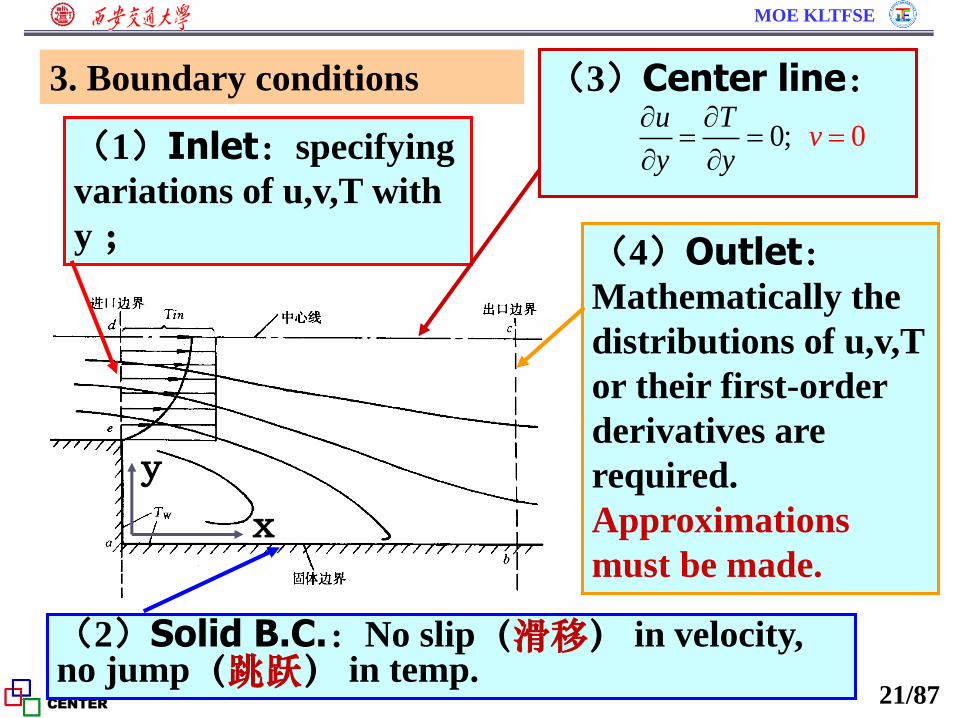
1.1.3 Example of mathematical formulation
1. Problem and assumptions
Convective heat transfer in a sudden expansion
region : 2D, steady- state, incompressible fluid,
constant properties, neglecting gravity and viscous
dissipation(耗散).
Solution
domain

MOE KLTFSE
20/87
2. Governing equations
0u v
x y
2 2
2 2
( ) ( ) 1( )
uu vu p u u
x y x x y
2 2
2 2
( ) ( ) 1( )
uv vv p v v
x y y x y
2 2
2 2
( ) ( )( )
uT vT T Ta
x y x y
p
ac
MOE KLTFSE
21/87
3. Boundary conditions
(2)Solid B.C.:No slip(滑移) in velocity, no jump(跳跃) in temp.
x
y
(1)Inlet:specifying
variations of u,v,T with
y ; (4)Outlet:Mathematically the
distributions of u,v,T
or their first-order
derivatives are
required.
Approximations
must be made.
(3)Center line:
00;
u Tv
y y

MOE KLTFSE
22/87
The right hand side :
Thus we have:
( 2 ) [ ( )] [ ( )] x
u uv w pdivU F
u
x y zx y x z x x
( )( ) ( )
udiv U div grad S
uu u
t
( )u u u
grad ux y z
i j k
( ( )) ( ) ( ) ( )u u u
div grad ux x y y z z
( ) ugradu Sdiv
( ) ( ) ( ) ( ) ( ) ( ) ( )
x
u v wdivU
x x y x z
u u u
x x y y xz
x
z x
pF
Navier-Stokes
( ( ))div grad u uS
( ) ( ) ( )( )
uu uv uwdiv uU
x y z
In the left hand side
Notes to Section 1.1

MOE KLTFSE
23/87
Gradient of a scalar (标量的梯度) is a vector:
( )u u u
grad u i j kx y z
Divergence of a vector (矢量的散度) is a scalar:
( ( )) ( )u u u
div grad u div i j kx y z
( ( )) ( ) ( ) ( )u u u
div grad ux x y y z z
( ( )) ( ) ( ) ( )u u u
div grad ux x y y z z
End of Notes to Section 1.1

MOE KLTFSE
24/87
1.2 Basic concepts of NHT and its application examples
1.2.1 Basic concepts of numerical solutions
based on continuum assumption
1.2.2 Classification of numerical solution methods
based on continuum assumption
1.2.3 Three fundamental approaches of
scientific research and their relationships
1.2.5 Some suggestions
1.2.4 Application examples

MOE KLTFSE
25/87
1.2.1 Basic concepts of numerical solutions based on continuum assumption(连续性假设)
1.2 Basic concepts of NHT and its application
examples
Replacing the fields of continuum variables (velocity,
temp. etc.) by sets (集合)of values at discrete(离散的)
points (nodes, 节点) (---Discretization of domain);
Establishing algebraic equations for these values at
the discrete points by some principles (---Discretization
of equations);
Solving the algebraic equations by computers to get
approximate solutions of the continuum variables
(---Solution of equation).

MOE KLTFSE
26/87
Discretizing
domain
Discretizing
equations
Solving
algebraic equations
Analyzing
numerical results Flow chart (流程图)

MOE KLTFSE
27/87
1. Finite difference method(FDM)
2. Finite volume method(FVM)
3. Finite element method(FEM)
4. Finite analytic method(FAM)
D B Spalding; S V Patankar
O C Zienkiewicz; 冯 康(Kang
Feng)
陈景仁(Ching Jen Chen)
5. Boundary element method(BEM) D B Brebbia
6. Spectral analysis method(SAM)
L F Richardson(1910),A Thom
1.2.2 Classification of numerical solution methods based on continuum assumption
(谱分析法)

MOE KLTFSE
28/87
Comparisons of FDM(a),FVM(b),FEM(c),FAM(d)
FDM
有限差分
All these methods need a grid system(网格系统):
1)Determination of grid positions;2)Establishing
the influence relationships between grids.
FVM
有限容积
FEM
有限元
FAM
有限分析

MOE KLTFSE
29/87
BEM (边界元)requires a basic solution, which greatly
limits its applications in convective problems.
SAM can only be applied to geometrically simple
cases.
Manole、Lage 1990-1992 statistics(统计):FVM --
-47%;adopted by most commercial softwares; Our
statistics of NHT in 2007 even much higher.

MOE KLTFSE
30/87
Theoretical analysis
Experimental research
Numerical simulation
1.2.3 Three fundamental approaches(方法) of
scientific research and their relationships
The starting point of numerical simulation for
physical problems is Fluid Dynamics. Thus it is often
called Computational Fluid Dynamics---CFD.

MOE KLTFSE
31/87
1. Theoretical analysis
Its importance should not be underestimated(低估).
It provides comparison basis for the verification(验证)
of numerical solutions.
Examples: The analytic solution of velocity from NS
equation for following case :
2
1 2 2
2
1 1 2 2
1 1
/ 1 ( / )
1 ( / ) /
u r r r r
u r r r r
u r

MOE KLTFSE
32/87
2. Experimental study
A basic research method: observation;properties
measurement; verification of numerical results
3.Numerical simulation
With the rapid development of computer
hardware(硬件), its importance and function will
become greater and greater.
Numerical simulation is an inter-discipline (交叉学科), and plays an important and un-replaceable role
in exploring (探索)unknowns, promoting (促进) the
development of science & technology, and for the
safety of national defense(国防安全).

MOE KLTFSE
33/87
Complicated
FF & HT
Atoms &
Molecules
Life
Science Numerical
Simulation
Historically,in 1985 the West Europe listed the
first commercial software-PHEONICS as the one which
was not allowed to sell to the communist countries.

MOE KLTFSE
34/87
In 2005 the USA President Advisory Board put
forward a suggestion to the president that in order to
keep competitive power (竞争力)of USA in the
world it should develops scientific computation.
In the year of 2006 the director of design department of Boeing , M. Grarett , reported to the US Congress(国会) indicating that the high performance computers have completely changed the way of designing Boeing airplane.
Numerical simulation plays
an important role in the
design of Boeing airplane

MOE KLTFSE
35/87
Example 1:Weather forecast-
Large scale vortex
Cloud Atlas sent back by a
meteorological satellite
Num. solution is the only way.
1.2.4 Application examples


MOE KLTFSE
37/87
Example 3:Hydraulic construction(水利建设)
The mud (泥)and sand(沙) content of our
Yellow River is about 35 kg/m3, ranking No. 1 in the world,
leading to following unpleasant situation: the ground floor
of some cities is lower than the riverbed(河床) of
Yellow River:Kai Feng-13m lower, Xin Xiang- 20m lower
In 2002 the idea of three yellow rivers was proposed:
Through 8 times of
modeling and simulation the
height of the riverbed was
averagely decreased by 1.5 m.
(1) Original YR;
(2)Numerical YR;
(3)Modele YR.

MOE KLTFSE
38/87
Example 4:Design of head shape of high-speed train
The front head shape of the high speed train is of great importance for its aerodynamic performance(空气动力学特性). Numerical wind tunnel is widely used to optimize the front head shape.


MOE KLTFSE
40/87
In the construction of gym :the chair material
cannot meet the requirement of fireproof(防火). A
decision should be made asap on whether such
material can be used. Numerical simulation was
adopted.


MOE KLTFSE
44/87
Example 6:House safety-Fire prediction
The major purpose is to guarantee(保证) that once fire
outbreak(火灾) occurs, the persons living in the house can
safely leave for outside within a certain amount of time.

MOE KLTFSE
Comparisons of predicted and simulated flow fields
Example 7:Heat transfer characteristics of large
electric current bar(电流母线)

MOE KLTFSE
46/87
Example 8:Shell-side simulation of helical baffle(螺旋折流板) heat exchanger
1.34
2.73
610

MOE KLTFSE
47/87
Example 9:Velocity and temperature distribution
simulation to improve design of air-conditioning
system
淮安市茂业时代广场项目空调系统CFD气流温度场分析
佛山金科大厦项目空调系统CFD气流温度场分析;
宁波甬邦大厦项目空调系统CFD 气流温度场分析

MOE KLTFSE
48/87
Temperature scale:℃
Out flow streamlines
Temperature distributions of 13F,14F,15F,16F Out flow stream
lines of 13F,14F,15F
Outflow air temperature clouds
Example 9:Velocity and temperature distribution simulation to improve design of air-conditioning system

MOE KLTFSE
49/87
Effect of floor number on the inflow temperature of air for condenser
10 12 14 16 18 20 22 24 26
35
36
37
38
39
40
41
42
43
44
45
温度
/℃
楼层
unit1
unit2
unit3
unit4
KS
The allowed upper limit is 43 ℃, thus the design is OK.

MOE KLTFSE
50/87
Visualization(可视化) of numerically predicted
results:
Example 9:Simulation of multiphase (多相) flow
2. Film boiling heat transfer (膜态沸腾);
3. Nucleate boiling in shallow liquid layer (浅液层中
的核态沸腾)
1. Breaking down of a dam (溃坝).

MOE KLTFSE
Evolution(演变) process of interface
0.0 0.5 1.0 1.5 2.0 2.5 3.01.0
1.5
2.0
2.5
3.0
3.5
4.0
r/L
t·(g/L)1/2
present simulation
Martin & Moyce
Base radius vs. time
51/87

MOE KLTFSE
4K 0 1 2 3 40
1
2
3
Nu
t(s)
数值模拟结果 Klimenko
5K
Experiment by Reimann
and Grigull (1975)
Klimenko correlation
Guo D.Z., Sun D.L.,Li Z.Y., Tao W.Q., Phase Change Heat Transfer Simulation for Boiling Bubbles Arising from a Vapor Film by VOSET Method. Numerical Heat Transfer, Part A: Applications, 2011, 59: 857-881
52/87

MOE KLTFSE
0.0 0.2 0.4 0.6 0.8 1.00
1x10⁴
2x10⁴
3x10⁴
4x10⁴
5x10⁴
时间/ s
热流密度
/ W
·m-2
深水条件 浅水条件
Shallow(浅)
liquid layer
Deep(深)
liquid layer Lin K, Tao WQ., Numerical simulation of nucleate boiling I shallow liquid. Asian Symposium on Computational Heat Transfer and Fluid Flow, 2015, Busan, Korea
Strong disturbance
caused by bubble
upward motion!
53/87
20160912

MOE KLTFSE
54/87
It is now widely accepted that an appropriate
combination of theoretical analysis, experimental study
and numerical simulation is the best approach for
modern scientific research.
With the further development of computer
hardware and numerical algorithm(算法), the
importance of numerical simulation will become
more and more important!
Summary

MOE KLTFSE
55/87
1.2.5 Some Suggestions
1. Understanding numerical methods from basic
characteristics of physical process;
2. Mastering complete picture and knowing every
details (明其全,析其微)for any numerical method;
3. Practicing simulation method by a computer;
4. Trying hard to analyze simulation results: rationality
(合理性) and regularity (规律性);
5. Adopting CSW(商业软件) with self-developed code.

MOE KLTFSE
56/87
Brief review of 2016-09-12 lecture key points
1. General governing eqs. and boundary conditions
of FF & HT problems
* *( )( ) ( )div U div grad S
t
Three kinds of B.C.:
(1) 1st :boundary value is known;
(2) 2nd :boundary heat flux is known
(3) 3rd :relationship between boundary value and
boundary 1st-order normal derivative(导数)is known
( ) ( )B B f
hT
Tn
T

MOE KLTFSE
57/87
2. Major concept of numerical simulation of HT &
FF problems
Solution of
algebraic eqs.
Domain discretization
Equation discretization
The differences in the three procedures(过程) lead to different numerical methods based on the continuum assumption.
----replacing the continuum domain by a number of discrete points, called node or grid, at which the values of velocity, temp., etc., are to be solved;
----replacing the governing equations by a number of algebraic equations for the nodes;
----solving the algebraic equations for the nodes by a computer.

MOE KLTFSE
58/87
1.3.1 From mathematical viewpoint(观点)
1.3.2 From physical viewpoint
1. General form of 2nd-order PDE(偏微分方程)
with two independent variables (二元)
2. Basic features(特点) of three types of PDEs
3. Relationship to numerical solution method
Conservative (守恒型) and non-conservative
1.3 Mathematical and physical classification of HT & FF problems and its effects on numerical solution
MOE KLTFSE
59/87
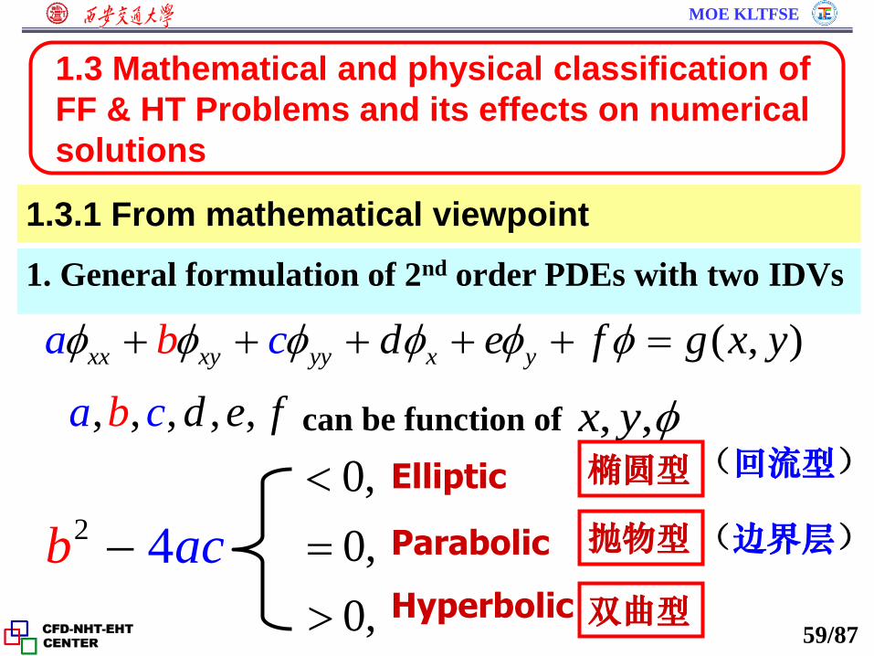
1.3.1 From mathematical viewpoint
1. General formulation of 2nd order PDEs with two IDVs
( , )xx xy yy x yd e f ga c x yb
, , , , ,ba c d e f , ,x y can be function of
24b ac
0, elliptic
0, parabolic
0, hyperbolic
椭圆型
抛物型
双曲型
Elliptic
Parabolic
Hyperbolic
(回流型)
(边界层)
1.3 Mathematical and physical classification of
FF & HT Problems and its effects on numerical
solutions

MOE KLTFSE
60/87
2. Basic feature of three types of PDEs
24 0,b ac having no real characteristic line;
24 0,b ac having one real characteristic line;
24 0,b ac having two real characteristic lines
leading to the difference in domain of dependence
(DOD,依赖区) and domain of influence (DOI,影响区);
DOD of a node is an area which determines the
value of a dependent variable at the node; DOI of a
node is an area within which the values of dependent
variable are affected by the node.
(没有实的特征线)

MOE KLTFSE
61/87
2
2
T T
t ya
2 2
2 2 2
1 1T T T
t ta c y
2 22
2 2C
t y
..xx xy yya b c
Elliptic
Parabolic Hyperbolic
DOI DOD DOD DOI DOD DOI

MOE KLTFSE
62/87
3. Relationship with numerical methods
(1)Elliptic:flow with
recirculation(回流),solution should be
conducted simultaneously
for the whole domain;
(2)Parabolic: flow without recirculation ,solution
can be conducted by marching method, greatly saving
computing time!。
Marching method

MOE KLTFSE
63/87
1.3.2 From physical viewpoint
1. Conservative (守恒型) vs. non-conservative(非守
恒型):
Conservative:those governing equations whose
convective term is expressed by divergence form(散度
形式) are called conservative governing equation .
Non-conservative: those governing equation whose
convective term is not expressed by divergence form is
called non-conservative governing equation .
These two concepts are only for numerical solution.

MOE KLTFSE
64/87
2. Conservative GE can guarantee the applicability(可用性) of physical conservation law within a finite (有限大小) volume.
( )( ) ( )
p
p T p
c Tdiv c TU div gradT S c
t
( ) ( ) ( )p p T p
V V V V
c T dv div c TU dv div gradT dv S c dvt
From Gauss theorem
( ) ( )V V
div gradT dv gradT ndA
( ) ( )p p
V V
div c TU dv c TU ndA
Dot product(点积)
MOE KLTFSE
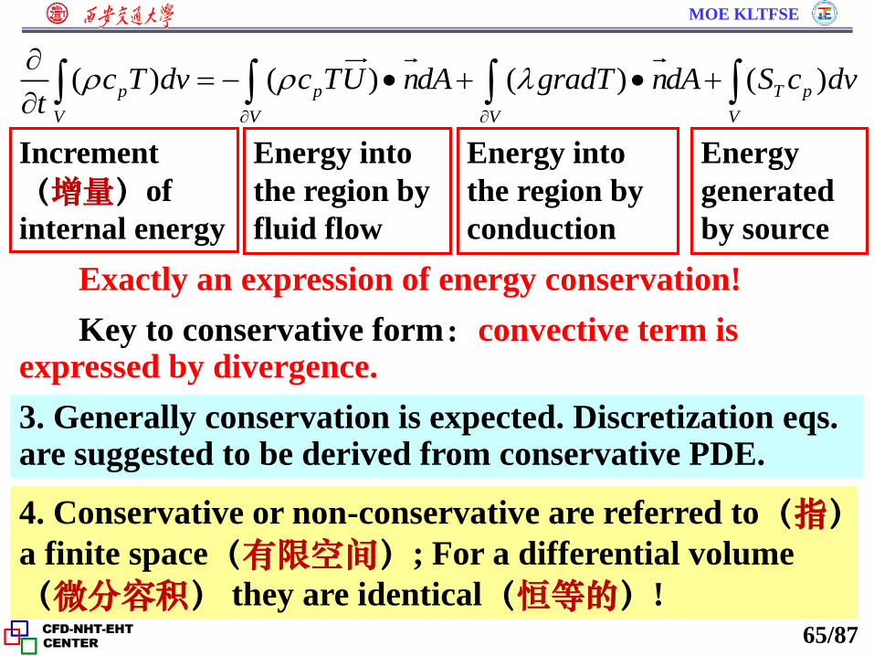
65/87
( ) ( ) ( ) ( )p p T p
V V V V
c T dv c TU ndA gradT ndA S c dvt
Increment
(增量)of
internal energy
Energy into
the region by
fluid flow
Energy into
the region by
conduction
Energy
generated
by source
Key to conservative form:convective term is expressed by divergence.
3. Generally conservation is expected. Discretization eqs. are suggested to be derived from conservative PDE.
4. Conservative or non-conservative are referred to(指)
a finite space(有限空间); For a differential volume
(微分容积) they are identical(恒等的)!
Exactly an expression of energy conservation!

MOE KLTFSE
66/87
1) For liquids:Up to micrometer scale (微米尺度)the
continuum based methods can be adopted.
2) For gases:Flow regimes(流态) are determined by
Knudsen number:ratio of molecular mean free path (分子平均自由程)over characteristic length(特征长度) :
KnL
Continuum
Slip, jump region
Transition(过渡)
Free molecule region
0.001
1.4.1 Applicable region of continuum assumption (连续性假设的适用范围)
1.4 Recent advances in numerical simulation of HT & HH problems
10
0.001 Kn 0.1
0.1 Kn 10

MOE KLTFSE
67/87
1) Macroscale(宏观层次)— Based on the
continuum assumption:FDM, FVM,FEM,FAM
2) Mesoscale(介观层次)— lattice-Boltzmann
method (LBM) ; Direct simulation of Monte Carlo
method(DSMC)
1.4.2 Numerical methods at three levels
LBM and DSMC belong to the mesoscale method:
both methods adopt a concept of computational
particle (计算粒子) ,which is much larger than a real
molecule, but can be treated as a molecule in some
sense(simulation molecule).

MOE KLTFSE
68/87
In MDS a domain contains a large number of
molecules and each molecule moves according to
Newton’s 2nd law of motion.
For numerical solutions of problems at different
scales there is most applicable(适用) method to each
scale.
3) Microscale(微观层次— Molecular dynamics
simulation (MDS).
There is one thing in common to the above three methods: macroscopic parameters (velocity, pressure, etc.) are obtained via some statistical (统计的) or averaged method.
Taking gas as an example, flow regime and related
numerical method can be classified as follows according
to the values of Knudson number: / L


MOE KLTFSE
70/87
Physical background, govern,eqs. and numer. methods
Ya-Ling He, Wen-Quan Tao, Multiscale simulations of heat transfer and fluid flow problems,
ASME J. Heat Transfer, 2012, 134:031018
Physics
Equa-
tions
Methods


MOE KLTFSE
72/87
In both engineering and nature, system or process
often covers several geometric or time scales. Such
system/process is called multiscale problem(多尺度问题).
Actually almost all problems have multiple scales
in nature(有多尺度特性);
Because of the limitations in the development of
science and technology , previous studies were mainly
concentrated at individual scale level.
1.4.3 Multiscale simulation
Turbulent flow and heat transfer is a typically
multiscale process where eddies(涡旋) at different
scales are included and interact with each other.

MOE KLTFSE
73/87 PEMFCs
The transport process in PEMFC (质子交换膜
燃料电池)covers several orders of geometries.

MOE KLTFSE
74/87
Transport process in PEMFC
Transport process in a PEFMC covers 3-4 orders of dimension.
Anode-阳极 Cathode-阴极 Catalyst-催化剂


MOE KLTFSE
76/87
In the present-day numerical simulation of PEMFC
usually FVM is adopted, and a number of empirical
parameters(经验参数) are involved with their values
being selected with great uncertain(不确定性). The V-
I curve is usually taken to verify a simulation model.
This leads to following unpleasant situation:
0.0 0.2 0.4 0.6 0.8 1.0 1.2 1.4
0.2
0.4
0.6
0.8
1.0
1.2
V
cell/
V
Iav/A cm-2
Group 1
Group 2
With two different sets of
empirical parameters we
may obtain almost the same
output curve.
Only multiscale simula-
tion can avoid(避免) such
an un-pleasant situation!
Tao W Q, Min C H, Liu X L, He Y L, Yin B H, Jiang W. Journal of Power
Source, 2006, 160:359-373

MOE KLTFSE
77/87
Information is coupled at
the interfaces of different
regions.
Full multiscale simulation for PEMFC
Flow in channel
by FVM
Transport in gas
diffusion layer by
LBM
Reaction in
catalyst layer by
MDS
Transport in
membrane by
MDS

MOE KLTFSE
78/87
1. Mesh-less method (无网格方法)
In the grid generation two kinds of data or
information are obtained:(1)positions of different
nodes ;(2)relationship between neighboring
nodes, influencing coefficient. The difficulty for grid
generation of complicated geometry is in the
establishment of the influencing coefficients.
1.4.4 Mesh-less method
In the mess-less method the positions of nodes are
still needed, however, the relationship between
neighboring nodes are not required. This so much
simplify the task of grid generation that researchers
call it “mesh-less” method.

MOE KLTFSE
79/87 Examples of sold large deformation
The conventional methods meet great difficulties
when large deformation (形变)occurs during the
simulation process. This happens in mechanical
manufacturing process.

MOE KLTFSE
80/87
The rapid development of high performance
supper computer(高性能超级计算机) has being
greatly enlarged the applicable region of numerical
simulation. Now we can say that almost every thing
can be simulated by computers, with different
reliability(可靠性) and accuracy(精度).
1.4.5 Supper-computer and parallel computation
My dream:there is one day in the future when
computer simulation becomes the major tool for
research and production design , and experiment
measurement is only needed for validate(验证)
some cases.

MOE KLTFSE
81/87
排名 制造商 总核数 峰值/实测性能
1 中国国防科技大学
6核Intel
186368
4701万亿次
2566万亿次(2566T)
2 Jaguar
(美洲豹)
6核AMD
224162
2331万亿次
1759万亿次
3 Nebulae
(星云)曙光
6核Intel
120640
2984万亿次
1271万亿次
4 Tsubame (燕子) NEC/HP公司
6核Intel
73278
2287.6万亿次
1192万亿次
5 Hopper(跳跃者) Cray
12核AMD
294912
1188.6万亿次
1054万亿次
2010年11月世界TOP500超级计算机
1G=109=10亿, 1T=1012=万亿, 1P=1015=1000万亿

MOE KLTFSE
82/87
排名 安装地点 制造商 峰值/实测 功耗
1 中国广州 国防科技大学
54900万亿(T)次
33860万亿次
17800kW
2
橡树林国家实验室 (Oak Ridge)
Cray 27110
17590
8200
3 劳伦斯国家实验室
IBM 20130
17170
7890
4 日本理化研究所
富士通 11280
10510
12660
5 阿贡国家实验室
IBM 10060
8580
3940
2013-11至2015-07世界TOP500超级计算机排名
1T=1012=万亿

MOE KLTFSE
83/87
Erratum
1. 第3页中间: -2/3 应改为 -2/3
4. 第7页 式(1-18)中右端: 应改为 p
3. 第4页倒数第3行: div U 应改为 2( )div U
本章作业为习题1-7(补充不可压,常物性的条件),与第二章一起上交。
5. 第9页倒数第3、4行右端:扩散项前的系数应为
2. 第3页倒数第3行: p
x
应改为 x
pF
x
倒数第1,2行仿此修改。
6. 式(1-6),(1-8)中漏了重力项。

MOE KLTFSE
84/87
Home Work 1
Problem 1-7
Adding following two assumptions:
Incompressible flow (不可压缩流体);
Constant thermo-physical properties(物性为常数)
Hand in with the home work of Chapter 2.
The pdf file of each chapter will be posted at our
group website!

MOE KLTFSE
85/87
A solid square having uniform temperature Th is
placed at center line of a two-dimensional parallel
plate channel as shown in figure below. Flow is fully
developed. The upper and lower side of the channel
is insulated and therefore you may assume that these
sides are adiabatic whereas outlet boundary is far
from the solid square. Fluid enters the channel with
a uniform temperature, Tin= C. Write down the
governing equations for steady state, incompressible
laminar flow with constant properties.
Problem 1-7

MOE KLTFSE
86/87
Also write down boundary conditions for the velocity
and temperature for the given domain (It is
preferable, at exit boundary, to take first derivative
zero). Flow is incompressible and material properties
are constants.

MOE KLTFSE
87/87
同舟共济 渡彼岸!
People in the same boat help each other to cross to the other bank, where….
本组网页地址:http://nht.xjtu.edu.cn 欢迎访问!
For convenience of discussion , a qq-group has been set up:
573633261