module - cheknowledge.files.wordpress.com · version 2 me, iit kharagpur space for a universal...

Version 2 ME, IIT Kharagpur

Module 3

Design for Strength


Lesson 1

Design for static loading


Instructional Objectives

At the end of this lesson, the students should be able to understand

• Types of loading on machine elements and allowable stresses.

• Concept of yielding and fracture.

• Different theories of failure.

• Construction of yield surfaces for failure theories.

• Optimize a design comparing different failure theories

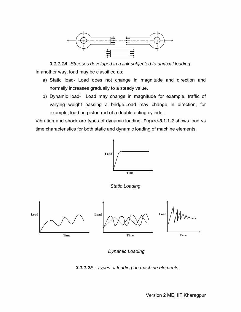
3.1.1 Introduction Machine parts fail when the stresses induced by external forces exceed their

strength. The external loads cause internal stresses in the elements and the

component size depends on the stresses developed. Stresses developed in a

link subjected to uniaxial loading is shown in figure-3.1.1.1. Loading may be due

to:

a) The energy transmitted by a machine element.

b) Dead weight.

c) Inertial forces.

d) Thermal loading.

e) Frictional forces.


Time

Load

Load

Time

Load

Time

Load

Time

3.1.1.1A- Stresses developed in a link subjected to uniaxial loading

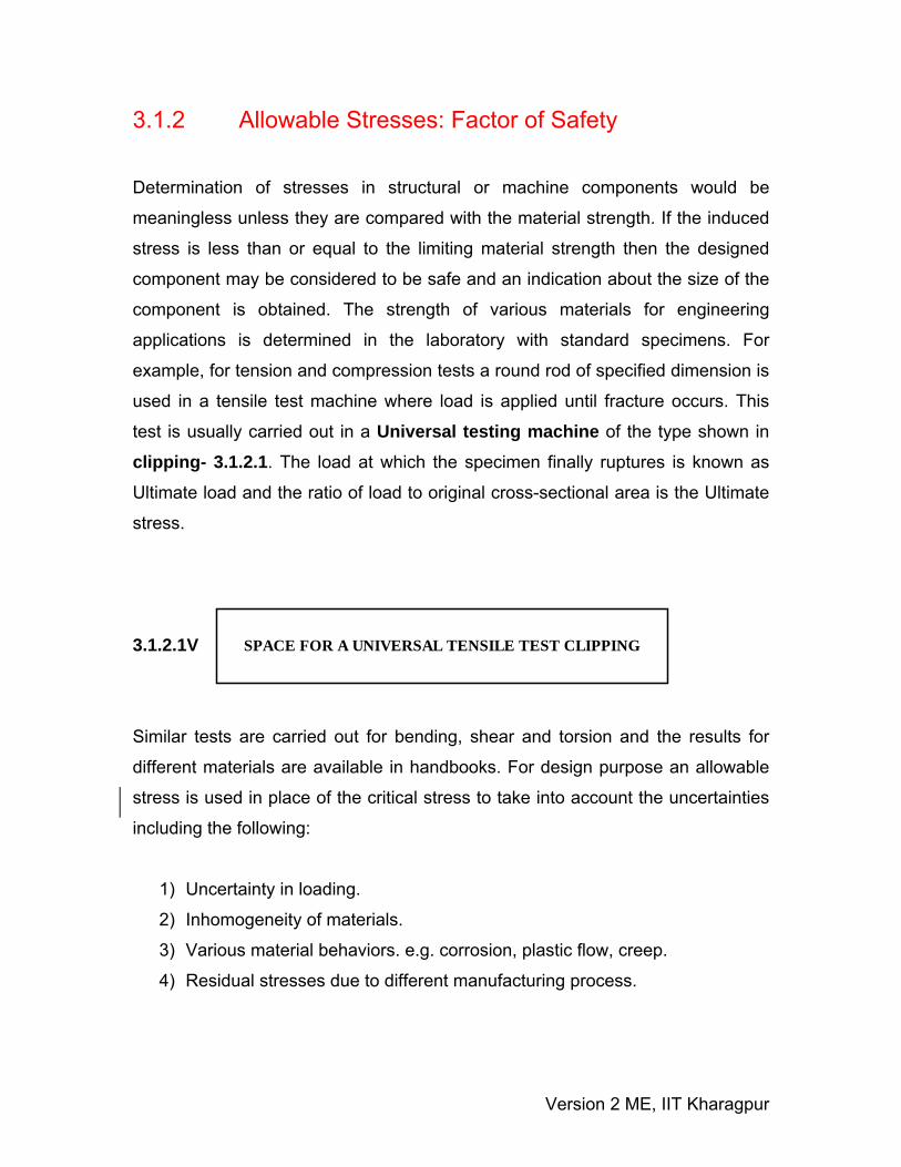
In another way, load may be classified as:

a) Static load- Load does not change in magnitude and direction and

normally increases gradually to a steady value.

b) Dynamic load- Load may change in magnitude for example, traffic of

varying weight passing a bridge.Load may change in direction, for

example, load on piston rod of a double acting cylinder.

Vibration and shock are types of dynamic loading. Figure-3.1.1.2 shows load vs

time characteristics for both static and dynamic loading of machine elements.

Static Loading

Dynamic Loading

3.1.1.2F - Types of loading on machine elements.


SPACE FOR A UNIVERSAL TENSILE TEST CLIPPING

3.1.2 Allowable Stresses: Factor of Safety Determination of stresses in structural or machine components would be

meaningless unless they are compared with the material strength. If the induced

stress is less than or equal to the limiting material strength then the designed

component may be considered to be safe and an indication about the size of the

component is obtained. The strength of various materials for engineering

applications is determined in the laboratory with standard specimens. For

example, for tension and compression tests a round rod of specified dimension is

used in a tensile test machine where load is applied until fracture occurs. This

test is usually carried out in a Universal testing machine of the type shown in

clipping- 3.1.2.1. The load at which the specimen finally ruptures is known as

Ultimate load and the ratio of load to original cross-sectional area is the Ultimate

stress.

3.1.2.1V

Similar tests are carried out for bending, shear and torsion and the results for

different materials are available in handbooks. For design purpose an allowable

stress is used in place of the critical stress to take into account the uncertainties

including the following:

1) Uncertainty in loading.

2) Inhomogeneity of materials.

3) Various material behaviors. e.g. corrosion, plastic flow, creep.

4) Residual stresses due to different manufacturing process.


UltimateStress F.S.AllowableStress

=

5) Fluctuating load (fatigue loading): Experimental results and plot- ultimate

strength depends on number of cycles.

6) Safety and reliability.

For ductile materials, the yield strength and for brittle materials the ultimate

strength are taken as the critical stress.

An allowable stress is set considerably lower than the ultimate strength. The ratio

of ultimate to allowable load or stress is known as factor of safety i.e.

The ratio must always be greater than unity. It is easier to refer to the ratio of

stresses since this applies to material properties.

3.1.3 Theories of failure When a machine element is subjected to a system of complex stress system, it is

important to predict the mode of failure so that the design methodology may be

based on a particular failure criterion. Theories of failure are essentially a set of

failure criteria developed for the ease of design.

In machine design an element is said to have failed if it ceases to perform its

function. There are basically two types of mechanical failure:

(a) Yielding- This is due to excessive inelastic deformation rendering the

machine

part unsuitable to perform its function. This mostly occurs in ductile

materials.

(b) Fracture- in this case the component tears apart in two or more parts. This

mostly occurs in brittle materials.

There is no sharp line of demarcation between ductile and brittle materials.

However a rough guideline is that if percentage elongation is less than 5%

then the material may be treated as brittle and if it is more than 15% then the


material is ductile. However, there are many instances when a ductile

material may fail by fracture. This may occur if a material is subjected to

(a) Cyclic loading.

(b) Long term static loading at elevated temperature.

(c) Impact loading.

(d) Work hardening.

(e) Severe quenching.

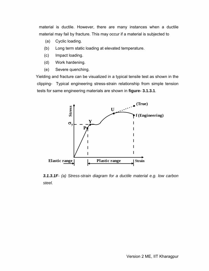
Yielding and fracture can be visualized in a typical tensile test as shown in the

clipping- Typical engineering stress-strain relationship from simple tension

tests for same engineering materials are shown in figure- 3.1.3.1.

3.1.3.1F- (a) Stress-strain diagram for a ductile material e.g. low carbon

steel.

Stre

ss

StrainPlastic rangeElastic range

(True)

f (Engineering)U

PYσy


3.1.3.1F- (b) Stress-strain diagram for low ductility.

3.1.3.1F- (c) Stress-strain diagram for a brittle material.

3.1.3.1F- (d) Stress-strain diagram for an elastic – perfectly plastic

material.

Stre

ss

Strain

Y

U(True)f (Engineering)

0.2 % offset

Strain

Stre

ss

f (Ultimate fracture)

σy

Stre

ss

Strain


SPACE FOR FATIGUE TEST CLIPPING

For a typical ductile material as shown in figure-3.1.3.1 (a) there is a definite yield

point where material begins to yield more rapidly without any change in stress

level. Corresponding stress is σy . Close to yield point is the proportional limit

which marks the transition from elastic to plastic range. Beyond elastic limit for an

elastic- perfectly plastic material yielding would continue without further rise in

stress i.e. stress-strain diagram would be parallel to parallel to strain axis beyond

the yield point. However, for most ductile materials, such as, low-carbon steel

beyond yield point the stress in the specimens rises upto a peak value known as

ultimate tensile stress σo . Beyond this point the specimen starts to neck-down

i.e. the reduction in cross-sectional area. However, the stress-strain curve falls till

a point where fracture occurs. The drop in stress is apparent since original cross-

sectional area is used to calculate the stress. If instantaneous cross-sectional

area is used the curve would rise as shown in figure- 3.1.3.1 (a) . For a material

with low ductility there is no definite yield point and usually off-set yield points are

defined for convenience. This is shown in figure-3.1.3.1. For a brittle material

stress increases linearly with strain till fracture occurs. These are demonstrated

in the clipping- 3.1.3.2 .

3.1.3.2V

3.1.4 Yield criteria

There are numerous yield criteria, going as far back as Coulomb (1773). Many of

these were originally developed for brittle materials but were later applied to

ductile materials. Some of the more common ones will be discussed briefly here.


σ2

σ1

b

+σy

a ..+σy

-σy

-σy

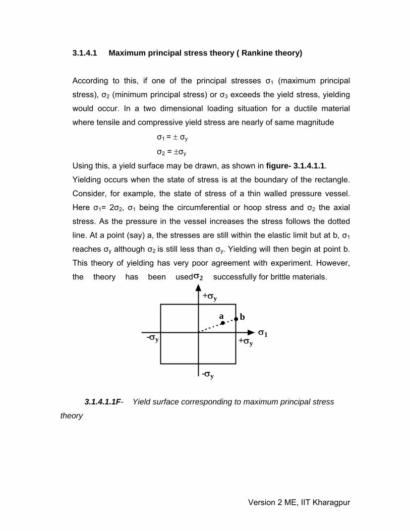
3.1.4.1 Maximum principal stress theory ( Rankine theory)

According to this, if one of the principal stresses σ1 (maximum principal

stress), σ2 (minimum principal stress) or σ3 exceeds the yield stress, yielding

would occur. In a two dimensional loading situation for a ductile material

where tensile and compressive yield stress are nearly of same magnitude

σ1 = ± σy

σ2 = ±σy

Using this, a yield surface may be drawn, as shown in figure- 3.1.4.1.1.

Yielding occurs when the state of stress is at the boundary of the rectangle.

Consider, for example, the state of stress of a thin walled pressure vessel.

Here σ1= 2σ2, σ1 being the circumferential or hoop stress and σ2 the axial

stress. As the pressure in the vessel increases the stress follows the dotted

line. At a point (say) a, the stresses are still within the elastic limit but at b, σ1

reaches σy although σ2 is still less than σy. Yielding will then begin at point b.

This theory of yielding has very poor agreement with experiment. However,

the theory has been used successfully for brittle materials.

3.1.4.1.1F- Yield surface corresponding to maximum principal stress

theory


( )

( )

1 1 2 1 2

2 2 1 2 1

1 1 2 0

2 2 1 0

1ε σ νσ σ σE1ε σ νσ σ σE

This gives, Eε σ νσ σ

Eε σ νσ σ

= − ≥

= − ≥

= − = ±

= − = ±

σ2

σ1-σy

-σy

σ2=σ0+νσ1

σ1=σ0+νσ2

+σy

+σy

3.1.4.2 Maximum principal strain theory (St. Venant’s theory) According to this theory, yielding will occur when the maximum principal strain

just exceeds the strain at the tensile yield point in either simple tension or

compression. If ε1 and ε2 are maximum and minimum principal strains

corresponding to σ1 and σ2, in the limiting case

The boundary of a yield surface in this case is thus given as shown in figure-3.1.4.2.1

3.1.4.2.1- Yield surface corresponding to maximum principal strain theory


1 2 y

2 3 y

3 1 y

σ σ σ

σ σ σ

σ σ σ

− = ±

− = ±

− = ±

1 2 y 1 2

1 2 y 1 2

2 y 2 1

1 y 1 2

1 y 1 2

2 y 2 1

σ σ σ if σ 0,σ 0

σ σ σ if σ 0,σ 0

σ σ if σ σ 0

σ σ if σ σ 0

σ σ if σ σ 0

σ σ if σ σ 0

− = > <

− = − < >

= > >

= − < <

= − > >

= − < <

σ2

σ1+σy-σy

+σy

-σy

3.1.4.3 Maximum shear stress theory ( Tresca theory) According to this theory, yielding would occur when the maximum shear

stress just exceeds the shear stress at the tensile yield point. At the tensile

yield point σ2= σ3 = 0 and thus maximum shear stress is σy/2. This gives us

six conditions for a three-dimensional stress situation:

3.1.4.3.1F- Yield surface corresponding to maximum shear stress

theory

In a biaxial stress situation ( figure-3.1.4.3.1) case, σ3 = 0 and this gives


( )1 1 2 2 3 3 y y1 1σ ε σ ε σ ε σ ε2 2

+ + =

σ2 σ1 σ

τ

( )1 1 2 2 3 3 y y1 1σ ε σ ε σ ε σ ε2 2

+ + =

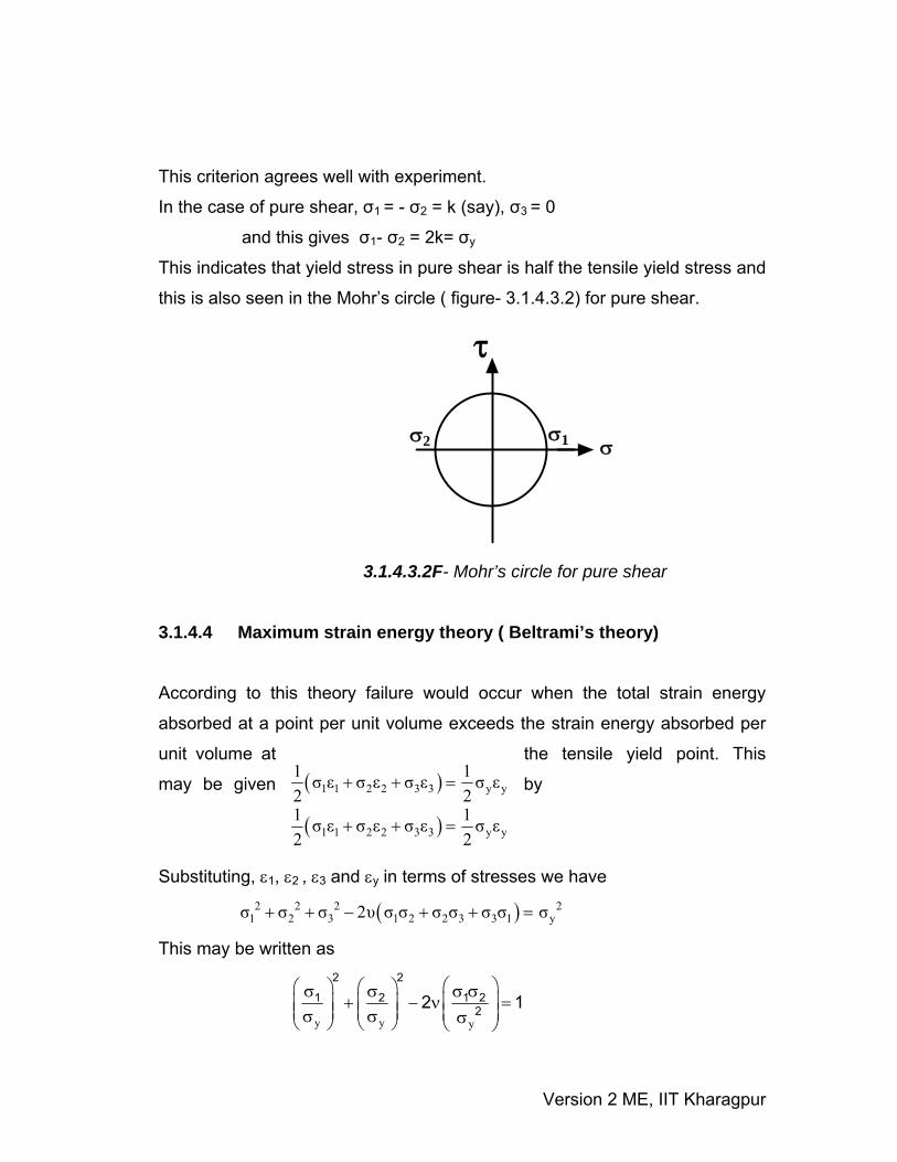
This criterion agrees well with experiment.

In the case of pure shear, σ1 = - σ2 = k (say), σ3 = 0

and this gives σ1- σ2 = 2k= σy

This indicates that yield stress in pure shear is half the tensile yield stress and

this is also seen in the Mohr’s circle ( figure- 3.1.4.3.2) for pure shear.

3.1.4.3.2F- Mohr’s circle for pure shear

3.1.4.4 Maximum strain energy theory ( Beltrami’s theory)

According to this theory failure would occur when the total strain energy

absorbed at a point per unit volume exceeds the strain energy absorbed per

unit volume at the tensile yield point. This

may be given by

Substituting, ε1, ε2 , ε3 and εy in terms of stresses we have

( )2 2 2 21 2 3 1 2 2 3 3 1 yσ σ σ 2υ σ σ σ σ σ σ σ+ + − + + =

This may be written as

y y y

2 2

1 2 1 222 1

⎛ ⎞⎛ ⎞ ⎛ ⎞σ σ σ σ⎜ ⎟+ − ν =⎜ ⎟ ⎜ ⎟⎜ ⎟ ⎜ ⎟ ⎜ ⎟σ σ σ⎝ ⎠ ⎝ ⎠ ⎝ ⎠


σ2

σ1

-σy

-σy

σy

σy

y E(1 )σ −νy E(1 )σ +ν

( )T 1 1 2 2 3 3 V av av1 3E σ ε σ ε σ ε and E σ ε2 2

= + + =

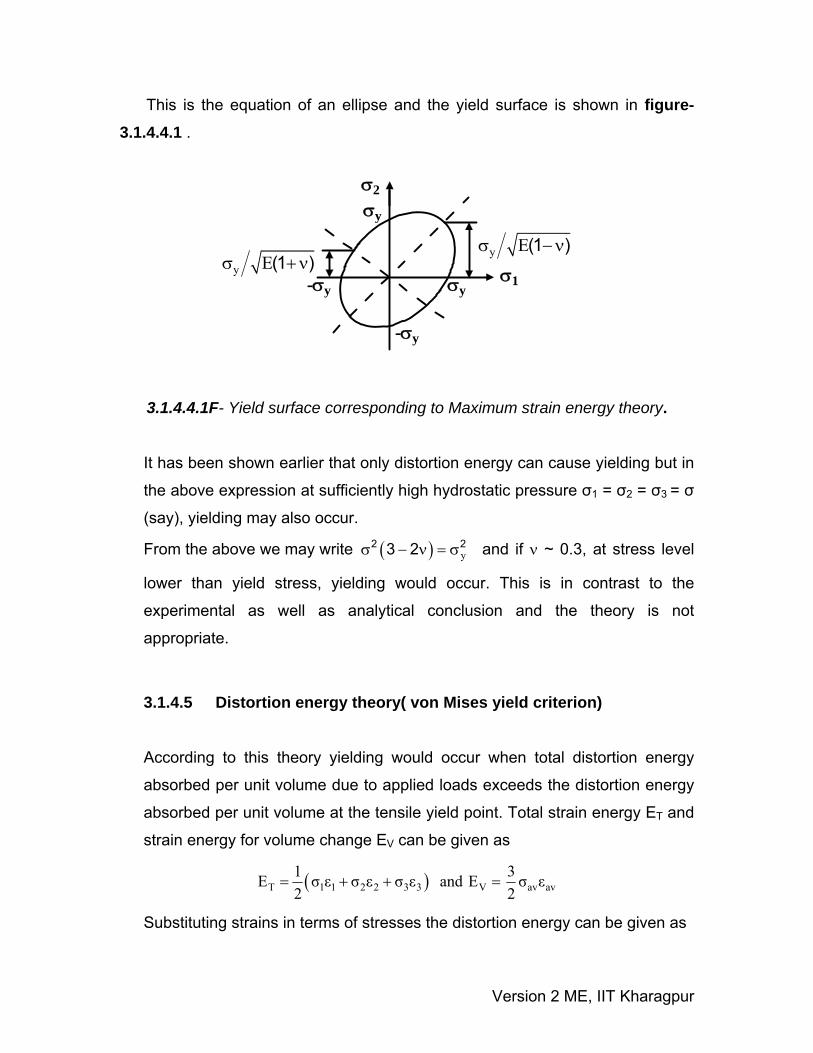
This is the equation of an ellipse and the yield surface is shown in figure-3.1.4.4.1 .

3.1.4.4.1F- Yield surface corresponding to Maximum strain energy theory.

It has been shown earlier that only distortion energy can cause yielding but in

the above expression at sufficiently high hydrostatic pressure σ1 = σ2 = σ3 = σ

(say), yielding may also occur.

From the above we may write ( ) y2 23 2σ − ν = σ and if ν ~ 0.3, at stress level

lower than yield stress, yielding would occur. This is in contrast to the

experimental as well as analytical conclusion and the theory is not

appropriate.

3.1.4.5 Distortion energy theory( von Mises yield criterion)

According to this theory yielding would occur when total distortion energy

absorbed per unit volume due to applied loads exceeds the distortion energy

absorbed per unit volume at the tensile yield point. Total strain energy ET and

strain energy for volume change EV can be given as

Substituting strains in terms of stresses the distortion energy can be given as


( ) ( ) ( )2 2 2 21 2 2 3 3 1 yσ σ σ σ σ σ 2σ− + − + − =

σ2

σ1

-σy

-σy

σy

σy

yσ

0.577 σy

45o

Ed = ET- EV = ( )2 2 21 2 3 1 2 2 3 3 1

2(1 ν) σ σ σ σ σ σ σ σ σ6E+

+ + − − −

At the tensile yield point, σ1 = σy , σ2 = σ3 = 0 which gives

2dy y

2(1 ν)E σ6E+

=

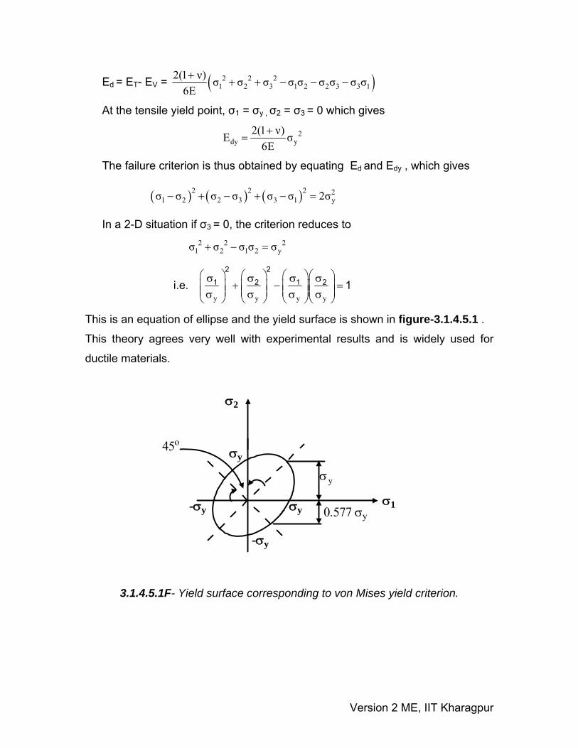
The failure criterion is thus obtained by equating Ed and Edy , which gives

In a 2-D situation if σ3 = 0, the criterion reduces to 2 2 2

1 2 1 2 yσ σ σ σ σ+ − =

i.e. y y y y

2 2

1 2 1 2 1⎛ ⎞ ⎛ ⎞ ⎛ ⎞⎛ ⎞σ σ σ σ

+ − =⎜ ⎟ ⎜ ⎟ ⎜ ⎟⎜ ⎟⎜ ⎟ ⎜ ⎟ ⎜ ⎟⎜ ⎟σ σ σ σ⎝ ⎠ ⎝ ⎠ ⎝ ⎠⎝ ⎠

This is an equation of ellipse and the yield surface is shown in figure-3.1.4.5.1 .

This theory agrees very well with experimental results and is widely used for

ductile materials.

3.1.4.5.1F- Yield surface corresponding to von Mises yield criterion.


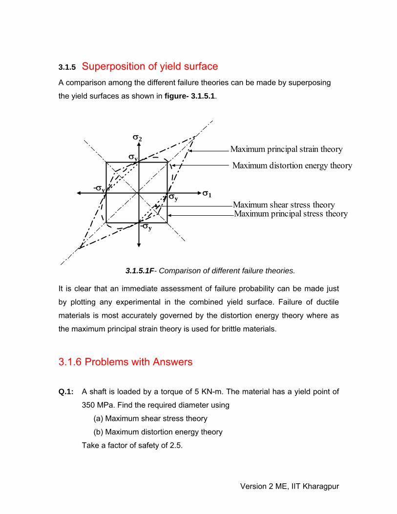
3.1.5 Superposition of yield surface A comparison among the different failure theories can be made by superposing

the yield surfaces as shown in figure- 3.1.5.1.

3.1.5.1F- Comparison of different failure theories. It is clear that an immediate assessment of failure probability can be made just

by plotting any experimental in the combined yield surface. Failure of ductile

materials is most accurately governed by the distortion energy theory where as

the maximum principal strain theory is used for brittle materials.

3.1.6 Problems with Answers

Q.1: A shaft is loaded by a torque of 5 KN-m. The material has a yield point of

350 MPa. Find the required diameter using

(a) Maximum shear stress theory

(b) Maximum distortion energy theory

Take a factor of safety of 2.5.

Maximum distortion energy theory

Maximum principal stress theory

σ2

-σy

σy

σyσ1

-σy

Maximum shear stress theory

Maximum principal strain theory


( ) ( ) ( ) ( )22 2 21 2 2 3 1 3 Yσ σ σ σ σ σ 2 σ F.S− + − + − =

A.1:

Torsional shear stress induced in the shaft due to 5 KN-m torque is

x xd

3

316 (5 10 )

τ =π

where d is the shaft diameter in m.

(b) Maximum shear stress theory,

x y2

2max 2

σ − σ⎛ ⎞τ = ± + τ⎜ ⎟

⎝ ⎠

Since σx = σy = 0, τmax=25.46x103/d3 = Y xxF S x

6350 102 . . 2 2.5σ

=

This gives d=71.3 mm.


In this case σ1 = 25.46x103/d3

σ2 = -25.46x103/d3

According to this theory,

Since σ3 = 0, substituting values of σ1 , σ2 and σY

D=68 mm.

Q.2: The state of stress at a point for a material is shown in the figure-3.1.6.1.

Find the factor of safety using (a) Maximum shear stress theory (b) Maximum

distortion energy theory. Take the tensile yield strength of the material as 400

MPa.

3.1.6.1F

τ=20 MPa

σx=40 MPa

σy=125 MPa


( ) ( ) ( ) ( )22 2 21 2 2 3 1 3 Yσ σ σ σ σ σ 2 σ F.S− + − + − =

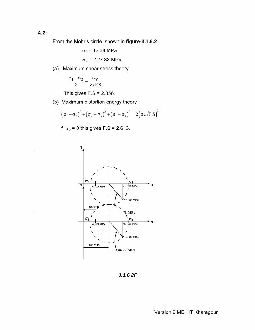
A.2: From the Mohr’s circle, shown in figure-3.1.6.2

σ1 = 42.38 MPa

σ2 = -127.38 MPa

(a) Maximum shear stress theory

Y

xF S1 2

2 2 .σ − σ σ

=

This gives F.S = 2.356.


If σ3 = 0 this gives F.S = 2.613.

3.1.6.2F

σ1σ2 σσx=20 MPa σy=120 MPa

τ=-20 MPa

τ

80 MPa44.72 MPa

σ1σ2 σσx=20 MPa σy=120 MPa

τ=-20 MPa

τ

80 MPa44.72 MPa


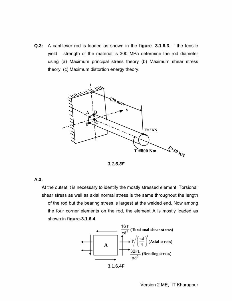
Q.3: A cantilever rod is loaded as shown in the figure- 3.1.6.3. If the tensile

yield strength of the material is 300 MPa determine the rod diameter

using (a) Maximum principal stress theory (b) Maximum shear stress

theory (c) Maximum distortion energy theory.

3.1.6.3F

A.3: At the outset it is necessary to identify the mostly stressed element. Torsional

shear stress as well as axial normal stress is the same throughout the length

of the rod but the bearing stress is largest at the welded end. Now among

the four corner elements on the rod, the element A is mostly loaded as

shown in figure-3.1.6.4

3.1.6.4F

120 mmx

P=10 KN

BA

C

F=2KN

T =800 Nm

D

A

Td3

16π

(Torsional shear stress)

dP2

4π⎛ ⎞

⎜ ⎟⎝ ⎠

(Axial stress)

FLd3

32π

(Bending stress)


Shear stress due to bending VQIt

is also developed but this is neglected

due to its small value compared to the other stresses. Substituting values

of T, P, F and L, the elemental stresses may be shown as in figure-3.1.6.5:

3.1.6.5F This gives the principal stress as

d d d d d

⎛ ⎞ ⎛ ⎞ ⎛ ⎞σ = + ± + +⎜ ⎟ ⎜ ⎟ ⎜ ⎟⎝ ⎠ ⎝ ⎠ ⎝ ⎠

2 2

1,2 2 3 2 3 31 12732 2445 1 12732 2445 40742 4

(a) Maximum principal stress theory,

Setting σ1 = σY we get d = 26.67 mm.

(b) Maximum shear stress theory,

Setting Y1 2

2 2σ − σ σ

= , we get d = 30.63 mm.

(c) Maximum distortion energy theory,

Setting ( ) ( ) ( ) ( )22 2 21 2 2 3 1 3 Yσ σ σ σ σ σ 2 σ− + − + − =

We get d = 29.36 mm.

d d2 312732 2445⎛ ⎞+⎜ ⎟⎝ ⎠

d⎛ ⎞⎜ ⎟⎝ ⎠3

4074


3.1.7 Summary of this Lesson Different types of loading and criterion for design of machine parts

subjected to static loading based on different failure theories have been

demonstrated. Development of yield surface and optimization of design

criterion for ductile and brittle materials were illustrated.


Module 3

Design for Strength


Lesson 2

Stress Concentration


Instructional Objectives At the end of this lesson, the students should be able to understand • Stress concentration and the factors responsible.

• Determination of stress concentration factor; experimental and theoretical

methods.

• Fatigue strength reduction factor and notch sensitivity factor.

• Methods of reducing stress concentration.

3.2.1 Introduction In developing a machine it is impossible to avoid changes in cross-section, holes,

notches, shoulders etc. Some examples are shown in figure- 3.2.1.1.

3.2.1.1F- Some typical illustrations leading to stress concentration.

Any such discontinuity in a member affects the stress distribution in the

neighbourhood and the discontinuity acts as a stress raiser. Consider a plate with

a centrally located hole and the plate is subjected to uniform tensile load at the

ends. Stress distribution at a section A-A passing through the hole and another

BEARING GEAR

KEY

COLLAR

GRUB SCREW


section BB away from the hole are shown in figure- 3.2.1.2. Stress distribution

away from the hole is uniform but at AA there is a sharp rise in stress in the

vicinity of the hole. Stress concentration factor tk is defined as 3t

avk σ= σ , where

σav at section AA is simply P t w b( 2 )− and Ptw1σ = . This is the theoretical or

geometric stress concentration factor and the factor is not affected by the

material properties.

3.2.1.2F- Stress concentration due to a central hole in a plate subjected to an

uni-axial loading.

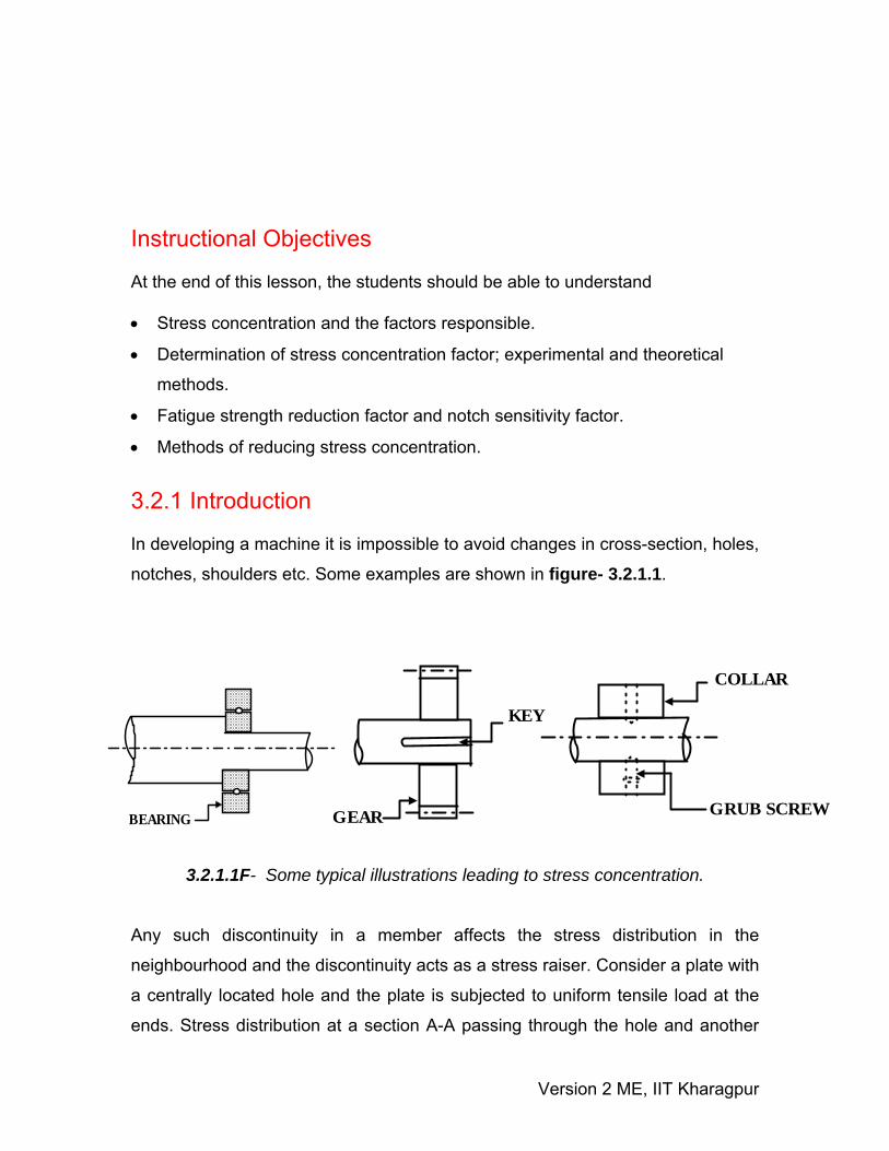
It is possible to predict the stress concentration factors for certain geometric

shapes using theory of elasticity approach. For example, for an elliptical hole in

an infinite plate, subjected to a uniform tensile stress σ1 (figure- 3.2.1.3), stress

distribution around the discontinuity is disturbed and at points remote from the

discontinuity the effect is insignificant. According to such an analysis

3 12b1a

⎛ ⎞σ = σ +⎜ ⎟⎝ ⎠

If a=b the hole reduces to a circular one and therefore 3 1σ = 3σ which gives tk =3.

If, however ‘b’ is large compared to ‘a’ then the stress at the edge of transverse

A A

B B

P

P

σ2

σ3

σ1

t

w

2b


crack is very large and consequently k is also very large. If ‘b’ is small compared

to a then the stress at the edge of a longitudinal crack does not rise and tk =1.

3.2.1.3F- Stress concentration due to a central elliptical hole in a plate subjected

to a uni-axial loading.

Stress concentration factors may also be obtained using any one of the following

experimental techniques:

1. Strain gage method

2. Photoelasticity method

3. Brittle coating technique

4. Grid method

For more accurate estimation numerical methods like Finite element analysis

may be employed.

Theoretical stress concentration factors for different configurations are available

in handbooks. Some typical plots of theoretical stress concentration factors and

rd ratio for a stepped shaft are shown in figure-3.2.1.4.

σ1

σ2

σ3

2a

2b


3.2.1.4F- Variation of theoretical stress concentration factor with r/d of a stepped

shaft for different values of D/d subjected to uni-axial loading (Ref.[2]).

In design under fatigue loading, stress concentration factor is used in modifying

the values of endurance limit while in design under static loading it simply acts as

stress modifier. This means Actual stress= tk ×calculated stress.

For ductile materials under static loading effect of stress concentration is not very

serious but for brittle materials even for static loading it is important.

It is found that some materials are not very sensitive to the existence of notches

or discontinuity. In such cases it is not necessary to use the full value of tk and


instead a reduced value is needed. This is given by a factor known as fatigue

strength reduction factor fk and this is defined as

fEndurance limit of notch free specimensk

Endurance limit of notched specimens=

Another term called Notch sensitivity factor, q is often used in design and this is

defined as

f

t

k 1qk 1−

=−

The value of ‘q’ usually lies between 0 and 1. If q=0, fk =1 and this indicates no

notch sensitivity. If however q=1, then fk = tk and this indicates full notch

sensitivity. Design charts for ‘q’ can be found in design hand-books and knowing

tk , fk may be obtained. A typical set of notch sensitivity curves for steel is

shown in figure- 3.2.1.5.

3.2.1.5F- Variation of notch sensitivity with notch radius for steels of different ultimate tensile strength (Ref.[2]).


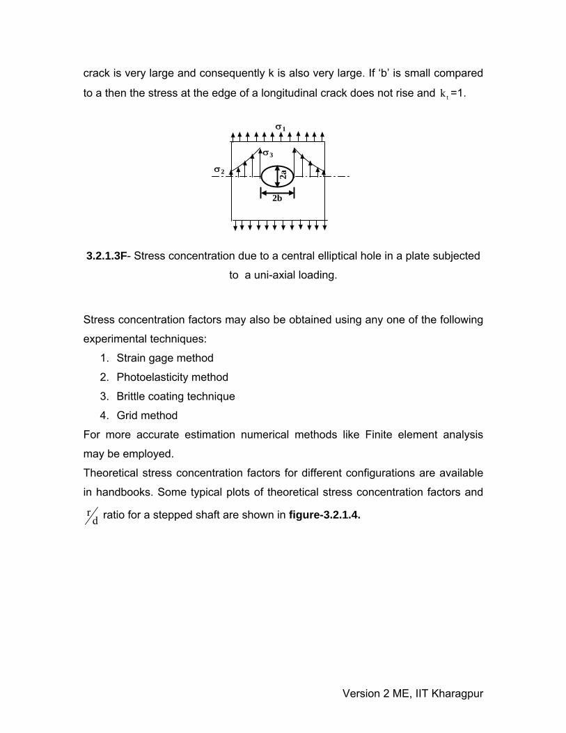
3.2.2 Methods of reducing stress concentration A number of methods are available to reduce stress concentration in machine

parts. Some of them are as follows:

1. Provide a fillet radius so that the cross-section may change gradually.

2. Sometimes an elliptical fillet is also used.

3. If a notch is unavoidable it is better to provide a number of small notches

rather than a long one. This reduces the stress concentration to a large extent.

4. If a projection is unavoidable from design considerations it is preferable to

provide a narrow notch than a wide notch.

5. Stress relieving groove are sometimes provided.

These are demonstrated in figure- 3.2.2.1.

(a) Force flow around a sharp corner Force flow around a corner with fillet: Low stress concentration. (b) Force flow around a large notch Force flow around a number of small notches: Low stress concentration.


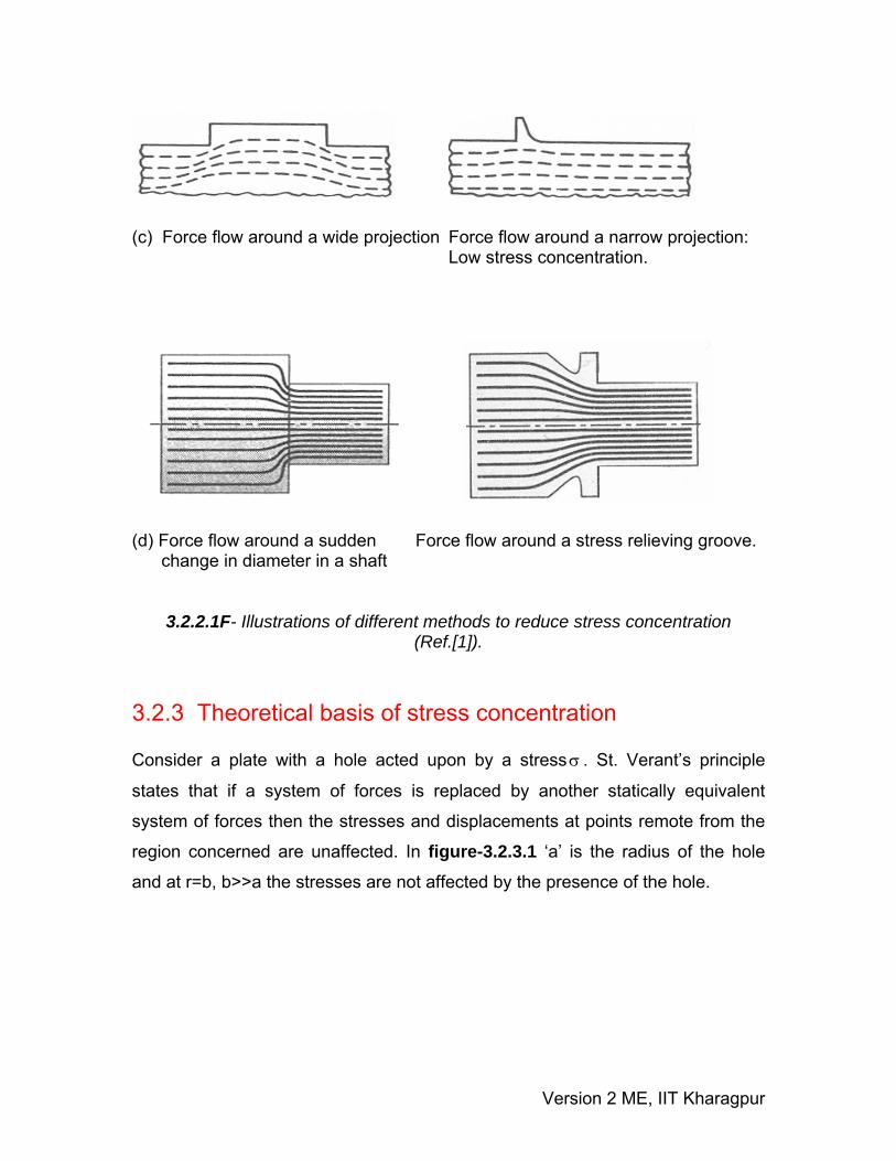
(c) Force flow around a wide projection Force flow around a narrow projection: Low stress concentration. (d) Force flow around a sudden Force flow around a stress relieving groove. change in diameter in a shaft

3.2.2.1F- Illustrations of different methods to reduce stress concentration (Ref.[1]).

3.2.3 Theoretical basis of stress concentration Consider a plate with a hole acted upon by a stressσ . St. Verant’s principle

states that if a system of forces is replaced by another statically equivalent

system of forces then the stresses and displacements at points remote from the

region concerned are unaffected. In figure-3.2.3.1 ‘a’ is the radius of the hole

and at r=b, b>>a the stresses are not affected by the presence of the hole.


3.2.3.1F- A plate with a central hole subjected to a uni-axial stress

Here, xσ = σ , y 0σ = , xy 0τ =

For plane stress conditions: 2 2

r x y xycos sin 2 cos sinσ = σ θ + σ θ + τ θ θ

2 2x y xysin cos 2 cos sinθσ = σ θ + σ θ − τ θ θ

( ) ( )2 2r x y xysin cos cos sinθτ = σ − σ θ θ + τ θ − θ

This reduces to

( )2r cos cos2 1 cos2

2 2 2σ σ σ

σ = σ θ = θ + = + θ

( )2sin 1 cos2 cos22 2 2θσ σ σ

σ = σ θ = − θ = − θ

r sin22θσ

τ = − θ

such that 1st component in rσ and θσ is constant and the second component

varies with θ . Similar argument holds for rθτ if we write rθτ = sin22σ

− θ . The

stress distribution within the ring with inner radius ir a= and outer radius or b=

due to 1st component can be analyzed using the solutions of thick cylinders and

y

xσ σa

b

P

Q


the effect due to the 2nd component can be analyzed following the Stress-function

approach. Using a stress function of the form ( )R r cos2φ = θ the stress

distribution due to the 2nd component can be found and it was noted that the

dominant stress is the Hoop Stress, given by 2 4

2 4a 3a1 1 cos2

2 r 2 rθ

⎛ ⎞ ⎛ ⎞σ σσ = + − + θ⎜ ⎟ ⎜ ⎟

⎝ ⎠ ⎝ ⎠

This is maximum at 2θ = ±π and the maximum value of 2 4

2 4a 3a2

2 r rθ

⎛ ⎞σσ = + +⎜ ⎟

⎝ ⎠

Therefore at points P and Q where r a= θσ is maximum and is given by 3θσ = σ

i.e. stress concentration factor is 3.


Q.1: The flat bar shown in figure- 3.2.4.1 is 10 mm thick and is pulled by a

force P producing a total change in length of 0.2 mm. Determine the

maximum stress developed in the bar. Take E= 200 GPa.

3.2.4.1F A.1: Total change in length of the bar is made up of three components and this

is given by

39

0.3 0.3 0.25 P0.2x100.025x0.01 0.05x0.01 0.025x0.01 200x10

− ⎡ ⎤= + +⎢ ⎥⎣ ⎦

This gives P=14.285 KN.

50 mm25 mm 25 mm P

300 mm 300 mm 250 mm

Fillet with stressconcentration factor 2.5

Fillet with stressconcentration factor 2.5

Hole with stressconcentration factor 2


Stress at the shoulder s16666k

(0.05 0.025)x0.01σ =

− where k=2.

This gives σh = 114.28 MPa.

Q.2: Find the maximum stress developed in a stepped shaft subjected to a

twisting moment of 100 Nm as shown in figure- 3.2.4.2. What would be the

maximum stress developed if a bending moment of 150 Nm is applied.

r = 6 mm

d = 30 mm

D = 40 mm.

3.2.4.2F

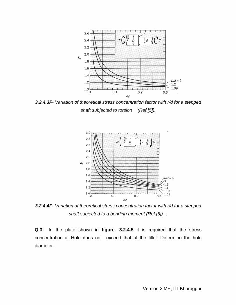
A.2: Referring to the stressconcentration plots in figure- 3.2.4.3 for stepped

shafts subjected to torsion for r/d = 0.2 and D/d = 1.33, Kt ≈ 1.23.

Torsional shear stress is given by 316T

dτ =

π. Considering the smaller diameter and

the stress concentration effect at the step, we have the maximum shear stress as

( )max t 3

16x100K0.03

τ =π

This gives τmax = 23.201 MPa.

Similarly referring to stress-concentration plots in figure- 3.2.4.4 for

stepped shaft subjected to bending , for r/d = 0.2 and D/d = 1.33, Kt ≈ 1.48

Bending stress is given by 332M

dσ =

π

Considering the smaller diameter and the effect of stress concentration at

the step, we have the maximum bending stress as

( )max t 3

32x150K0.03

σ =π

This gives σmax = 83.75 MPa.


3.2.4.3F- Variation of theoretical stress concentration factor with r/d for a stepped

shaft subjected to torsion (Ref.[5]).

3.2.4.4F- Variation of theoretical stress concentration factor with r/d for a stepped

shaft subjected to a bending moment (Ref.[5]) .

Q.3: In the plate shown in figure- 3.2.4.5 it is required that the stress

concentration at Hole does not exceed that at the fillet. Determine the hole

diameter.


3.2.4.5F A.3: Referring to stress-concentration plots for plates with fillets under axial

loading (figure- 3.2.4.6 ) for r/d = 0.1 and D/d = 2,

stress concentration factor, Kt ≈ 2.3.

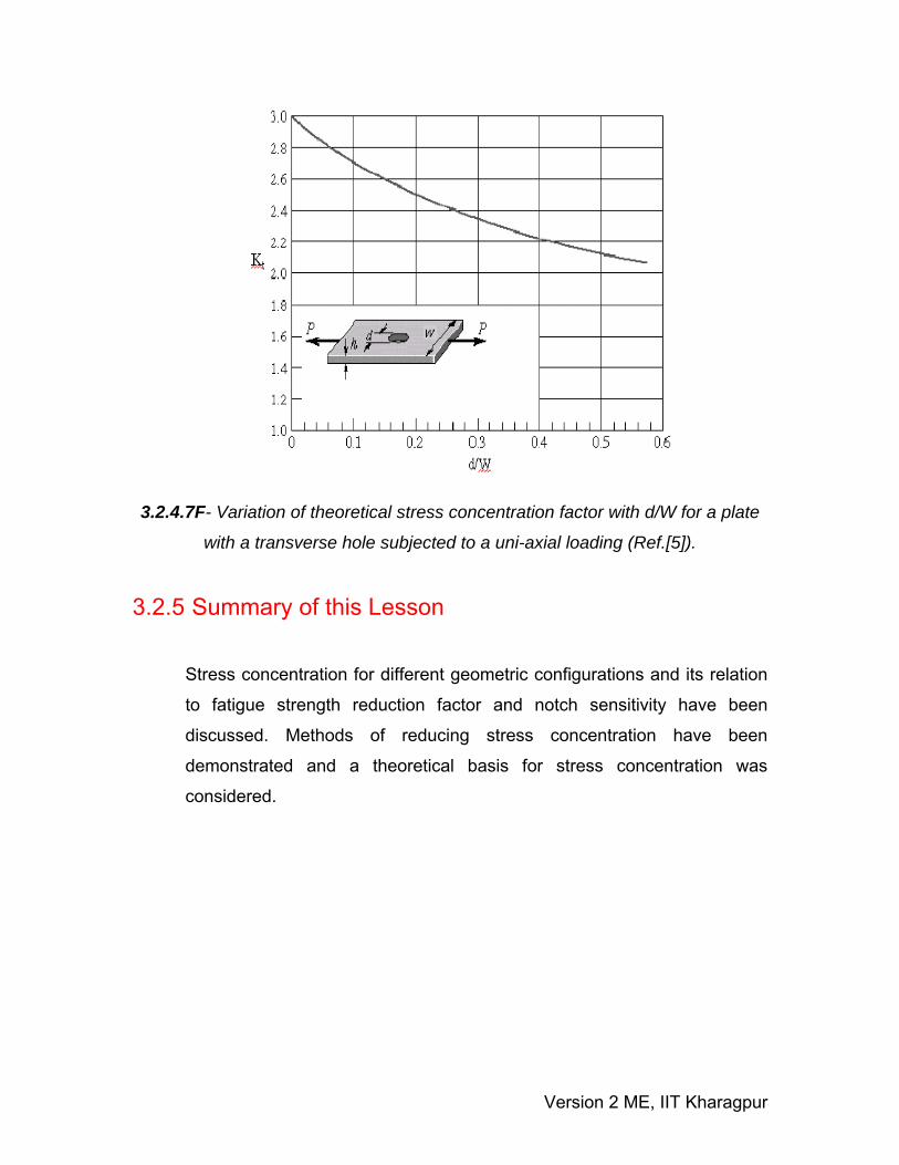
From stress concentration plots for plates with a hole of diameter ‘d’ under axial

loading ( figure- 3.2.4.7 ) we have for Kt = 2.3, d′/D = 0.35.

This gives the hole diameter d′ = 35 mm.

3.2.4.6F- Variation of theoretical stress concentration factor with r/d for a plate

with fillets subjected to a uni-axial loading (Ref.[5]).

100 mm d' P50 mm

5 mm


3.2.4.7F- Variation of theoretical stress concentration factor with d/W for a plate

with a transverse hole subjected to a uni-axial loading (Ref.[5]).

3.2.5 Summary of this Lesson

Stress concentration for different geometric configurations and its relation

to fatigue strength reduction factor and notch sensitivity have been

discussed. Methods of reducing stress concentration have been

demonstrated and a theoretical basis for stress concentration was

considered.

Module 3

Design for Strength Version 2 ME, IIT Kharagpur

Lesson 3

Design for dynamic loading


Instructional Objectives At the end of this lesson, the students should be able to understand • Mean and variable stresses and endurance limit.

• S-N plots for metals and non-metals and relation between endurance limit

and ultimate tensile strength.

• Low cycle and high cycle fatigue with finite and infinite lives.

• Endurance limit modifying factors and methods of finding these factors. 3.3.1 Introduction Conditions often arise in machines and mechanisms when stresses fluctuate

between a upper and a lower limit. For example in figure-3.3.1.1, the fiber on the

surface of a rotating shaft subjected to a bending load, undergoes both tension

and compression for each revolution of the shaft.

-

+

TP

3.3.1.1F- Stresses developed in a rotating shaft subjected to a bending load.

Any fiber on the shaft is therefore subjected to fluctuating stresses. Machine

elements subjected to fluctuating stresses usually fail at stress levels much

below their ultimate strength and in many cases below the yield point of the

material too. These failures occur due to very large number of stress cycle and

are known as fatigue failure. These failures usually begin with a small crack


which may develop at the points of discontinuity, an existing subsurface crack or

surface faults. Once a crack is developed it propagates with the increase in

stress cycle finally leading to failure of the component by fracture. There are

mainly two characteristics of this kind of failures:

(a) Progressive development of crack.

(b) Sudden fracture without any warning since yielding is practically absent.

Fatigue failures are influenced by

(i) Nature and magnitude of the stress cycle.

(ii) Endurance limit.

(iii) Stress concentration.

(iv) Surface characteristics.

These factors are therefore interdependent. For example, by grinding and

polishing, case hardening or coating a surface, the endurance limit may be

improved. For machined steel endurance limit is approximately half the ultimate

tensile stress. The influence of such parameters on fatigue failures will now be

discussed in sequence.

3.3.2 Stress cycle A typical stress cycle is shown in figure- 3.3.2.1 where the maximum, minimum,

mean and variable stresses are indicated. The mean and variable stresses are

given by

minmean

miniable

σ + σσ =

σ − σσ =

max

maxvar

2

2


σmax

σmin

σm

σv

Time

Stre

ss

3.3.2.1F- A typical stress cycle showing maximum, mean and variable stresses.

3.3.3 Endurance limit Figure- 3.3.3.1 shows the rotating beam arrangement along with the specimen.

Machined and polished surface

W

(a) Beam specimen (b) Loading arrangement

3.3.3.1F- A typical rotating beam arrangement.

The loading is such that there is a constant bending moment over the specimen

length and the bending stress is greatest at the center where the section is

smallest. The arrangement gives pure bending and avoids transverse shear


since bending moment is constant over the length. Large number of tests with

varying bending loads are carried out to find the number of cycles to fail. A typical

plot of reversed stress (S) against number of cycles to fail (N) is shown in figure-3.3.3.2. The zone below 103 cycles is considered as low cycle fatigue, zone

between 103 and 106 cycles is high cycle fatigue with finite life and beyond 106

cycles, the zone is considered to be high cycle fatigue with infinite life.

Low cycle fatigue High cycle fatigue

Finite life Infinite life

S

103 106

N

Endurance limit

3.3.3.2F- A schematic plot of reversed stress (S) against number of cycles to fail (N) for steel.

The above test is for reversed bending. Tests for reversed axial, torsional or

combined stresses are also carried out. For aerospace applications and non-

metals axial fatigue testing is preferred. For non-ferrous metals there is no knee

in the curve as shown in figure- 3.3.3.3 indicating that there is no specified

transition from finite to infinite life.


S

N

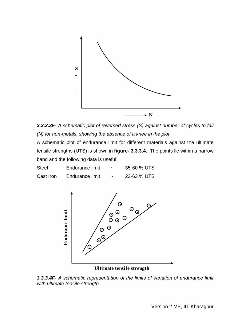
3.3.3.3F- A schematic plot of reversed stress (S) against number of cycles to fail

(N) for non-metals, showing the absence of a knee in the plot.

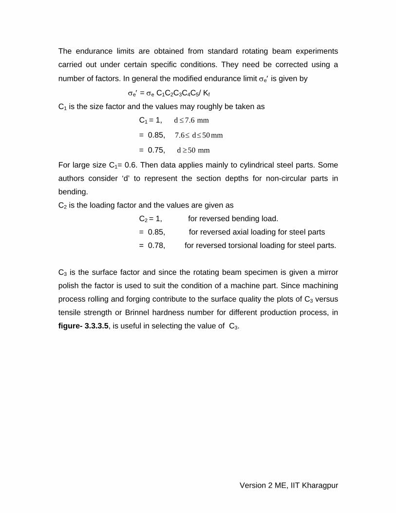
A schematic plot of endurance limit for different materials against the ultimate

tensile strengths (UTS) is shown in figure- 3.3.3.4. The points lie within a narrow

band and the following data is useful:

Steel Endurance limit ~ 35-60 % UTS

Cast Iron Endurance limit ~ 23-63 % UTS

End

uran

ce li

mit

Ultimate tensile strength

.

...

..

.. ..

.

.

.

.

3.3.3.4F- A schematic representation of the limits of variation of endurance limit with ultimate tensile strength.


The endurance limits are obtained from standard rotating beam experiments

carried out under certain specific conditions. They need be corrected using a

number of factors. In general the modified endurance limit σe′ is given by

σe′ = σe C1C2C3C4C5/ Kf

C1 is the size factor and the values may roughly be taken as

C1 = 1, d 7.6 mm≤

= 0.85, 7.6 d 50 mm≤ ≤

= 0.75, d 50 mm≥

For large size C1= 0.6. Then data applies mainly to cylindrical steel parts. Some

authors consider ‘d’ to represent the section depths for non-circular parts in

bending.

C2 is the loading factor and the values are given as

C2 = 1, for reversed bending load.

= 0.85, for reversed axial loading for steel parts

= 0.78, for reversed torsional loading for steel parts.

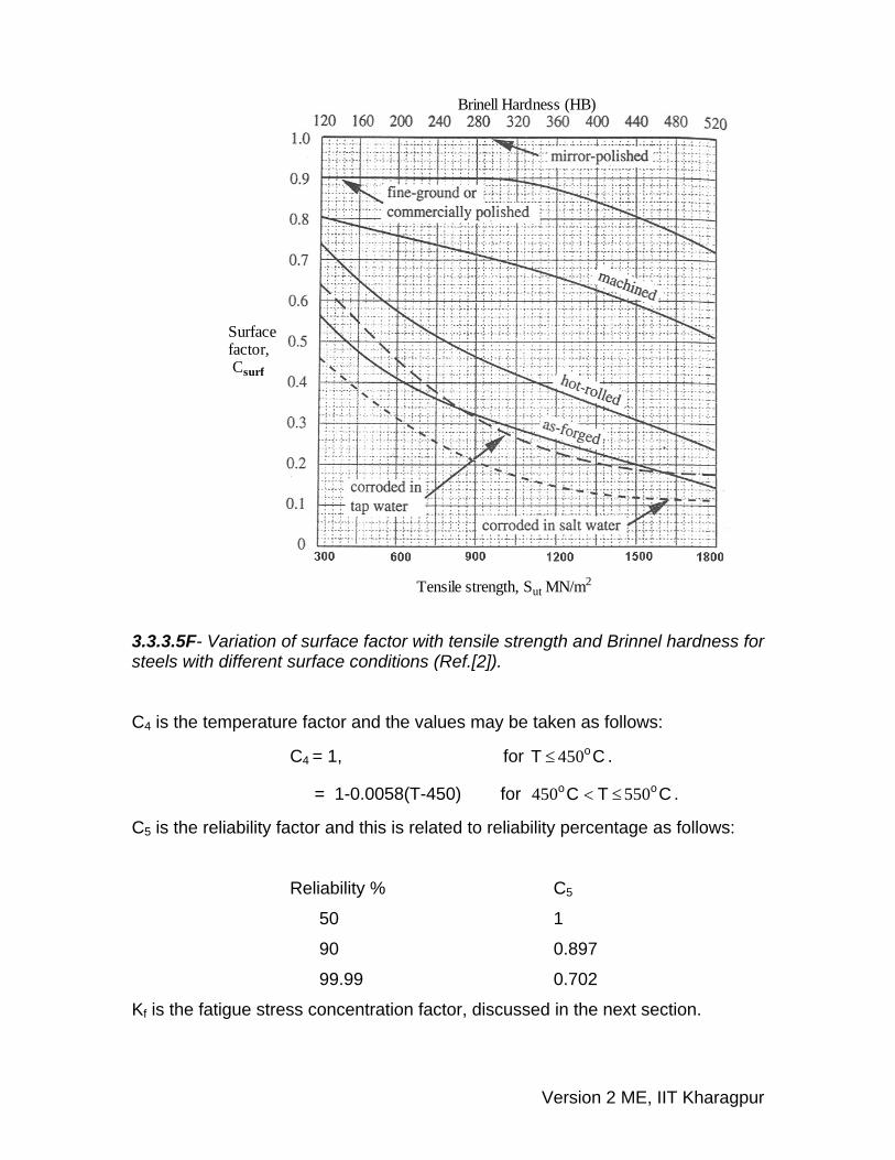
C3 is the surface factor and since the rotating beam specimen is given a mirror

polish the factor is used to suit the condition of a machine part. Since machining

process rolling and forging contribute to the surface quality the plots of C3 versus

tensile strength or Brinnel hardness number for different production process, in

figure- 3.3.3.5, is useful in selecting the value of C3.


Tensile strength, Sut MN/m2

Surfacefactor,Csurf

Brinell Hardness (HB)

3.3.3.5F- Variation of surface factor with tensile strength and Brinnel hardness for steels with different surface conditions (Ref.[2]). C4 is the temperature factor and the values may be taken as follows:

C4 = 1, for . 450oT C≤

= 1-0.0058(T-450) for . 450 550o oC T C< ≤

C5 is the reliability factor and this is related to reliability percentage as follows:

Reliability % C5

50 1

90 0.897

99.99 0.702

Kf is the fatigue stress concentration factor, discussed in the next section.


3.3.4 Stress concentration Stress concentration has been discussed in earlier lessons. However, it is

important to realize that stress concentration affects the fatigue strength of

machine parts severely and therefore it is extremely important that this effect be

considered in designing machine parts subjected to fatigue loading. This is done

by using fatigue stress concentration factor defined as

fEndurance limit of a notch free specimenk

Endurance limit of a notched specimen=

The notch sensitivity ‘q’ for fatigue loading can now be defined in terms of Kf and

the theoretical stress concentration factor Kt and this is given by

−=

−f

t

K 1qK 1

The value of q is different for different materials and this normally lies between 0

to 0.7. The index is small for ductile materials and it increases as the ductility

decreases. Notch sensitivities of some common materials are given in table- 3.3.4.1 .

3.3.4.1T- Notch sensitivity of some common engineering materials.

Material Notch sensitivity index

C-30 steel- annealed 0.18

C-30 steel- heat treated and drawn at

480oC

0.49

C-50 steel- annealed 0.26


480oC

0.50


480oC

0.57

Stainless steel- annealed 0.16

Cast iron- annealed 0.00-0.05

copper- annealed 0.07

Duraluminium- annealed 0.05-0.13


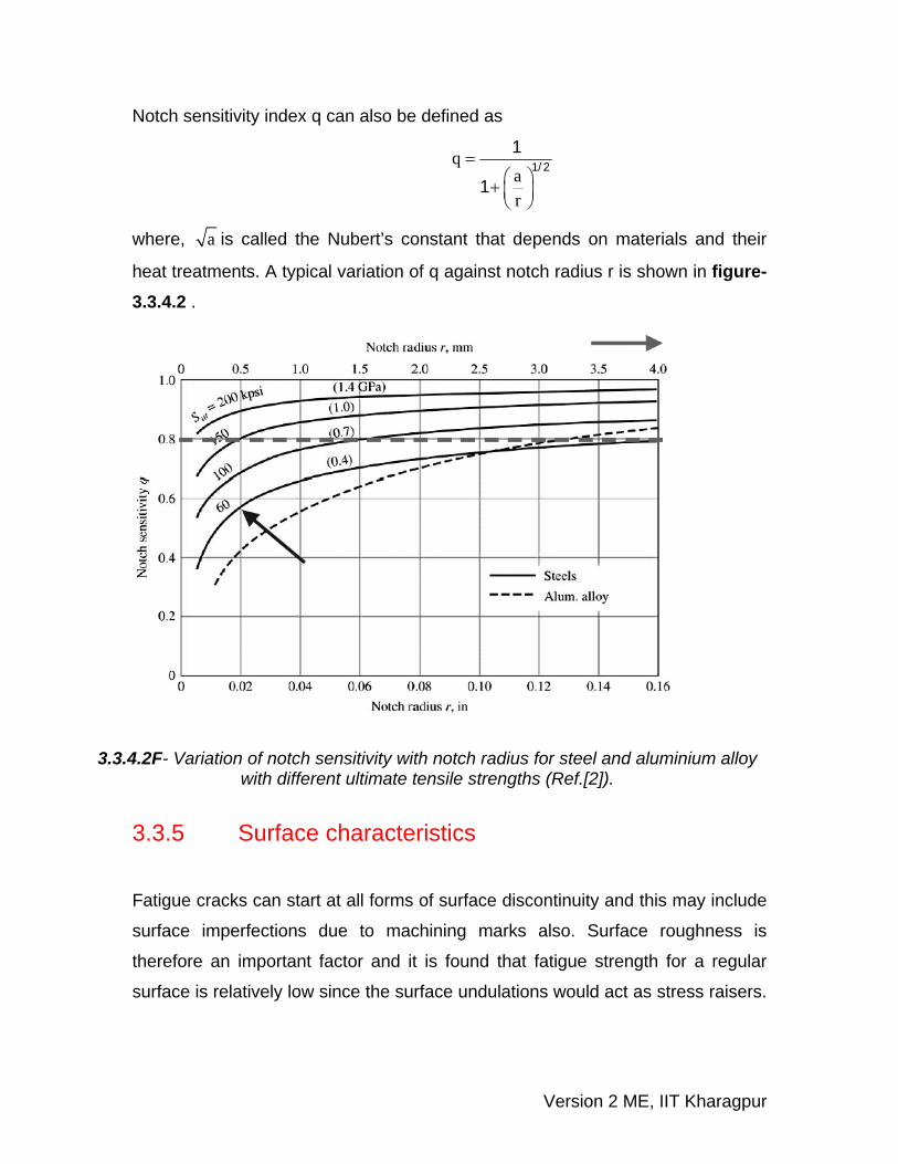
Notch sensitivity index q can also be defined as

qar

=⎛ ⎞+ ⎜ ⎟⎝ ⎠

1/ 21

1

where, a is called the Nubert’s constant that depends on materials and their

heat treatments. A typical variation of q against notch radius r is shown in figure- 3.3.4.2 .

3.3.4.2F- Variation of notch sensitivity with notch radius for steel and aluminium alloy with different ultimate tensile strengths (Ref.[2]).

3.3.5 Surface characteristics Fatigue cracks can start at all forms of surface discontinuity and this may include

surface imperfections due to machining marks also. Surface roughness is

therefore an important factor and it is found that fatigue strength for a regular

surface is relatively low since the surface undulations would act as stress raisers.


It is, however, impractical to produce very smooth surfaces at a higher machining

cost.

Another important surface effect is due to the surface layers which may be

extremely thin and stressed either in tension or in compression. For example,

grinding process often leaves surface layers highly stressed in tension. Since

fatigue cracks are due to tensile stress and they propagate under these

conditions and the formation of layers stressed in tension must be avoided.

There are several methods of introducing pre-stressed surface layer in

compression and they include shot blasting, peening, tumbling or cold working by

rolling. Carburized and nitrided parts also have a compressive layer which

imparts fatigue strength to such components. Many coating techniques have

evolved to remedy the surface effects in fatigue strength reductions.


Q.1: A rectangular stepped steel bar is shown in figure-3.3.6.1. The bar is

loaded in bending. Determine the fatigue stress-concentration factor if

ultimate stress of the materials is 689 MPa.

r = 5mm D = 50 mm d = 40 mm b = 1 mm

3.3.6.1F A.1: From the geometry r/d = 0.125 and D/d = 1.25.

From the stress concentration chart in figure- 3.2.4.6

Stress- concentration factor Kt ≈ 1.7

From figure- 3.3.4.2

Notch sensitivity index, q ≈ 0.88

The fatigue stress concentration factor Kf is now given by

Kf = 1+q (Kt -1) =1.616


3.3.7 Summary of this Lesson

Design of components subjected to dynamic load requires the concept of

variable stresses, endurance limit, low cycle fatigue and high cycle fatigue

with finite and infinite life. The relation of endurance limit with ultimate

tensile strength is an important guide in such design. The endurance limit

needs be corrected for a number of factors such as size, load, surface

finish, temperature and reliability. The methods for finding these factors

have been discussed and demonstrated in an example.



Module 3

Design for Strength


Lesson 4

Low and high cycle fatigue


Instructional Objectives At the end of this lesson, the students should be able to understand • Design of components subjected to low cycle fatigue; concept and necessary

formulations.

• Design of components subjected to high cycle fatigue loading with finite life;

concept and necessary formulations.

• Fatigue strength formulations; Gerber, Goodman and Soderberg equations.

3.4.1 Low cycle fatigue This is mainly applicable for short-lived devices where very large overloads may

occur at low cycles. Typical examples include the elements of control systems in

mechanical devices. A fatigue failure mostly begins at a local discontinuity and

when the stress at the discontinuity exceeds elastic limit there is plastic strain.

The cyclic plastic strain is responsible for crack propagation and fracture.

Experiments have been carried out with reversed loading and the true stress-

strain hysteresis loops are shown in figure-3.4.1.1. Due to cyclic strain the

elastic limit increases for annealed steel and decreases for cold drawn steel. Low

cycle fatigue is investigated in terms of cyclic strain. For this purpose we consider

a typical plot of strain amplitude versus number of stress reversals to fail for steel

as shown in figure-3.4.1.2.


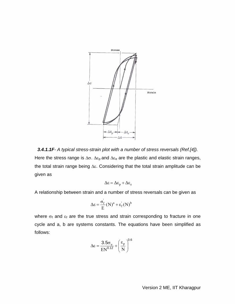
3.4.1.1F- A typical stress-strain plot with a number of stress reversals (Ref.[4]).

Here the stress range is Δσ. Δεp and Δεe are the plastic and elastic strain ranges,

the total strain range being Δε. Considering that the total strain amplitude can be

given as

p eΔε Δε Δε= +

A relationship between strain and a number of stress reversals can be given as

'

a ' bff

σΔε (N) ε (N)E

= +

where σf and εf are the true stress and strain corresponding to fracture in one

cycle and a, b are systems constants. The equations have been simplified as

follows:

pu

NEN

0.6

0.123.5 ε⎛ ⎞σ

Δε = + ⎜ ⎟⎝ ⎠


In this form the equation can be readily used since σu, εp and E can be measured

in a typical tensile test. However, in the presence of notches and cracks

determination of total strain is difficult.

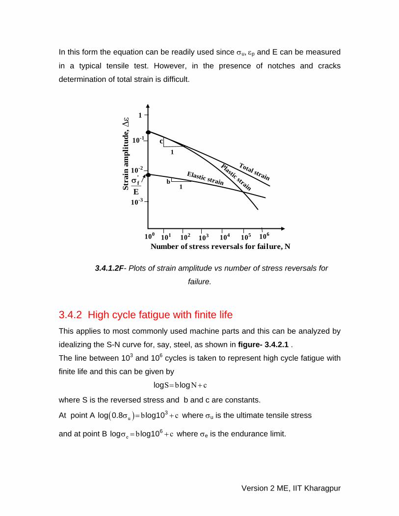
3.4.1.2F- Plots of strain amplitude vs number of stress reversals for

failure.

3.4.2 High cycle fatigue with finite life This applies to most commonly used machine parts and this can be analyzed by

idealizing the S-N curve for, say, steel, as shown in figure- 3.4.2.1 .

The line between 103 and 106 cycles is taken to represent high cycle fatigue with

finite life and this can be given by

S b N c= +log log

where S is the reversed stress and b and c are constants.

At point A ( )u b c3log 0.8 log10σ = + where σu is the ultimate tensile stress

and at point B e b cσ = +6log log10 where σe is the endurance limit.

Total strainElastic strain

Plastic strain

c

b

101 102 103 104 105 106

10-3

10-2

10-1

1

Number of stress reversals for failure, N

Stra

in a

mpl

itud

e,

'f

Eσ

100

1

1

Δε


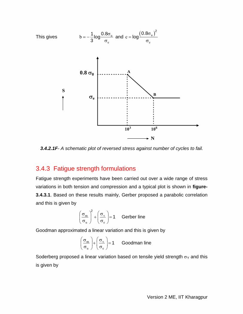
This gives u

eb

σ= −

σ0.81 log

3 and ( )u

ec

σ=

σ

20.8log

3.4.2.1F- A schematic plot of reversed stress against number of cycles to fail.

3.4.3 Fatigue strength formulations Fatigue strength experiments have been carried out over a wide range of stress

variations in both tension and compression and a typical plot is shown in figure- 3.4.3.1. Based on these results mainly, Gerber proposed a parabolic correlation

and this is given by

vm

u e

2

1⎛ ⎞ ⎛ ⎞σσ

+ =⎜ ⎟ ⎜ ⎟σ σ⎝ ⎠ ⎝ ⎠ Gerber line

Goodman approximated a linear variation and this is given by

vm

u e1

⎛ ⎞ ⎛ ⎞σσ+ =⎜ ⎟ ⎜ ⎟σ σ⎝ ⎠ ⎝ ⎠

Goodman line

Soderberg proposed a linear variation based on tensile yield strength σY and this

is given by

A

B

103 106

σe

0.8 σ0

S

N


vm

y e

⎛ ⎞ ⎛ ⎞σσ+ =⎜ ⎟ ⎜ ⎟⎜ ⎟σ σ⎝ ⎠⎝ ⎠

1 Soderberg line

Here, σm and σv represent the mean and fluctuating components respectively.

3.4.3.1F- A schematic diagram of experimental plots of variable stress against mean stress and Gerber, Goodman and Soderberg lines.


Q.1: A grooved shaft shown in figure- 3.4.4.1 is subjected to rotating-bending

load. The dimensions are shown in the figure and the bending moment is

30 Nm. The shaft has a ground finish and an ultimate tensile strength of

1000 MPa. Determine the life of the shaft.

r = 0.4 mm D = 12 mm d = 10 mm

3.4.4.1F

o

o oo

o

oo o

o o

oo oo o

o

o

o

ooo

o

o

o

oo

oo

o

o

o

o

o

o

o

o

o

oV

aria

ble

stre

ss,σ

v

Mean stress, σmCompressive stress Tensile stress

σe

σuσy

Gerber line

Goodman line

Soderberg line


A.1:

Modified endurance limit, σe′ = σe C1C2C3C4C5/ Kf

Here, the diameter lies between 7.6 mm and 50 mm : C1 = 0.85

The shaft is subjected to reversed bending load: C2 = 1

From the surface factor vs tensile strength plot in figure- 3.3.3.5

For UTS = 1000 MPa and ground surface: C3 = 0.91

Since T≤ 450oC, C4 = 1

For high reliability, C5 = 0.702.

From the notch sensitivity plots in figure- 3.3.4.2 , for r=0.4 mm and UTS

= 1000 MPa, q = 0.78

From stress concentration plots in figure-3.4.4.2, for r/d = 0.04 and D/d =

1.2, Kt = 1.9. This gives Kf = 1+q (Kt -1) = 1.702.

Then, σe′ = σex 0.89x 1x 0.91x 1x 0.702/1.702 = 0.319 σe

For steel, we may take σe = 0.5 σUTS = 500 MPa and then we have

σe′ = 159.5 MPa.

Bending stress at the outermost fiber, b 332Mσπd

=

For the smaller diameter, d=0.01 mm, bσ 305 MPa=

Since 'b eσ σ> life is finite.

For high cycle fatigue with finite life,

log S = b log N + C

where, e

b σ= −

σ00.81 log

3 ' = x

− =−1 0.8 1000log 0.2333 159.5

( )u

ec

σ=

σ

20.8log

' = ( )x

=20.8 1000

log 3.60159.5

Therefore, finite life N can be given by

N=10-c/b S1/b if 103 ≤ N ≤ 106.

Since the reversed bending stress is 306 MPa,

N = 2.98x 109 cycles.


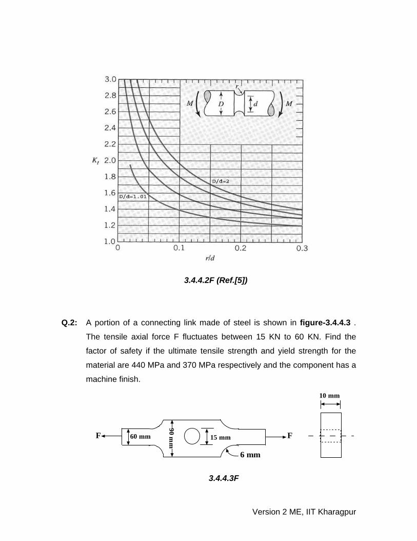
3.4.4.4F

3.4.4.2F (Ref.[5]) Q.2: A portion of a connecting link made of steel is shown in figure-3.4.4.3 .

The tensile axial force F fluctuates between 15 KN to 60 KN. Find the

factor of safety if the ultimate tensile strength and yield strength for the

material are 440 MPa and 370 MPa respectively and the component has a

machine finish.

3.4.4.3F

90 mm60 mm 15 mm F

6 mm

10 mm

F


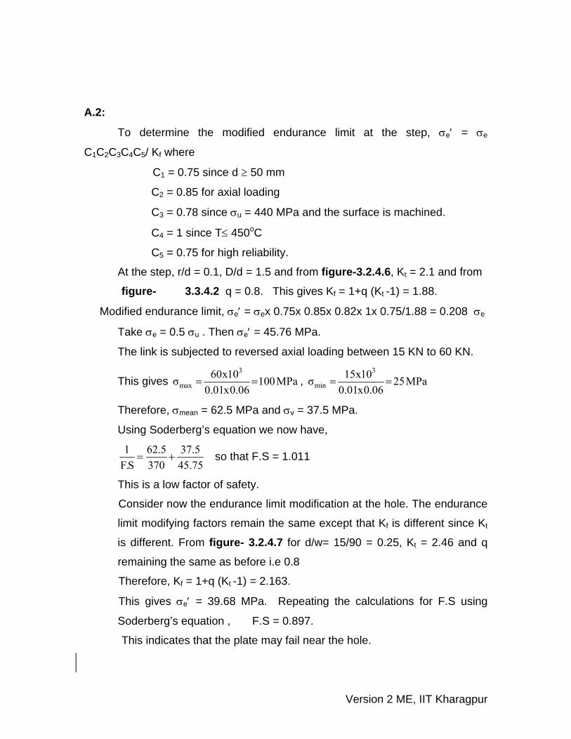
A.2:

To determine the modified endurance limit at the step, σe′ = σe

C1C2C3C4C5/ Kf where

C1 = 0.75 since d ≥ 50 mm

C2 = 0.85 for axial loading

C3 = 0.78 since σu = 440 MPa and the surface is machined.

C4 = 1 since T≤ 450oC

C5 = 0.75 for high reliability.

At the step, r/d = 0.1, D/d = 1.5 and from figure-3.2.4.6, Kt = 2.1 and from

figure- 3.3.4.2 q = 0.8. This gives Kf = 1+q (Kt -1) = 1.88.

Modified endurance limit, σe′ = σex 0.75x 0.85x 0.82x 1x 0.75/1.88 = 0.208 σe

Take σe = 0.5 σu . Then σe′ = 45.76 MPa.

The link is subjected to reversed axial loading between 15 KN to 60 KN.

This gives 3

max60x10σ 100MPa

0.01x0.06= = ,

3

min15x10σ 25MPa

0.01x0.06= =

Therefore, σmean = 62.5 MPa and σv = 37.5 MPa.

Using Soderberg’s equation we now have,

1 62.5 37.5F.S 370 45.75

= + so that F.S = 1.011

This is a low factor of safety.

Consider now the endurance limit modification at the hole. The endurance

limit modifying factors remain the same except that Kf is different since Kt

is different. From figure- 3.2.4.7 for d/w= 15/90 = 0.25, Kt = 2.46 and q

remaining the same as before i.e 0.8

Therefore, Kf = 1+q (Kt -1) = 2.163.

This gives σe′ = 39.68 MPa. Repeating the calculations for F.S using

Soderberg’s equation , F.S = 0.897.

This indicates that the plate may fail near the hole.


Q.3: A 60 mm diameter cold drawn steel bar is subjected to a completely

reversed torque of 100 Nm and an applied bending moment that varies

between 400 Nm and -200 Nm. The shaft has a machined finish and has a

6 mm diameter hole drilled transversely through it. If the ultimate tensile

stress σu and yield stress σy of the material are 600 MPa and 420 MPa

respectively, find the factor of safety.

A.3: The mean and fluctuating torsional shear stresses are

τm = 0 ; ( )v 3

16x100τπx 0.06

= = 2.36 MPa.

and the mean and fluctuating bending stresses are

( )m 3

32x100σπx 0.06

= = 4.72 MPa; ( )v 3

32x300σπx 0.06

= = 14.16 MPa.

For finding the modifies endurance limit we have,

C1 = 0.75 since d > 50 mm

C2 = 0.78 for torsional load

= 1 for bending load

C3 = 0.78 since σu = 600 MPa and the surface is machined ( figure-

3.4.4.2).

C4 = 1 since T≤ 450oC

C5 = 0.7 for high reliability.

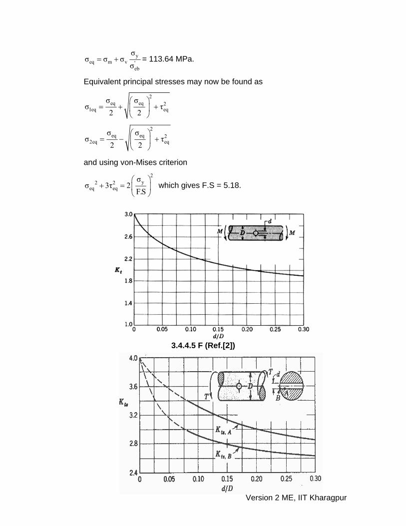
and Kf = 2.25 for bending with d/D =0.1 (from figure- 3.4.4.5 )

= 2.9 for torsion on the shaft surface with d/D = 0.1 (from figure- 3.4.4.6 )

This gives for bending σeb′ = σex 0.75x1x 0.78x 1x 0.7/2.25 = 0.182 σe

For torsion σes′ = σesx 0.75x0.78x 0.78x 1x 0.7/2.9 = 0.11 σe

And if σe = 0.5 σu = 300 MPa, σeb′ =54.6 MPa; σes′ = 33 MPa

We may now find the equivalent bending and torsional shear stresses as:

yeq m v '

es

ττ τ τ

σ= + = 15.01 MPa ( Taking τy = 0.5 σy = 210 MPa)


yeq m v '

eb

σσ σ σ

σ= + = 113.64 MPa.

Equivalent principal stresses may now be found as

2eq eq 2

1eq eq

2eq eq 2

2eq eq

σ σσ τ

2 2

σ σσ τ

2 2

⎛ ⎞= + +⎜ ⎟

⎝ ⎠

⎛ ⎞= − +⎜ ⎟

⎝ ⎠

and using von-Mises criterion

2

y2 2eq eq

σσ 3τ 2

F.S⎛ ⎞

+ = ⎜ ⎟⎝ ⎠

which gives F.S = 5.18.

3.4.4.5 F (Ref.[2])


3.4.4.6 F (Ref.[2])

3.4.5 Summary of this Lesson The simplified equations for designing components subjected to both low

cycle and high cycle fatigue with finite life have been explained and

methods to determine the component life have been demonstrated. Based

on experimental evidences, a number of fatigue strength formulations are

available and Gerber, Goodman and Soderberg equations have been

discussed. Methods to determine the factor of safety or the safe design

stresses under variable loading have been demonstrated.


3.4.6 Reference for Module-3

1) Design of machine elements by M.F.Spotts, Prentice hall of India,1991.

2) Machine design-an integrated approach by Robert L. Norton, Pearson

Education Ltd, 2001.

3) A textbook of machine design by P.C.Sharma and D.K.Agarwal,

S.K.Kataria and sons, 1998.

4) Mechanical engineering design by Joseph E. Shigley, McGraw Hill,

1986.

5) Fundamentals of machine component design, 3rd edition, by Robert C.

Juvinall and Kurt M. Marshek, John Wiley & Sons, 2000.

module - cheknowledge.files.wordpress.com · version 2 me, iit kharagpur space for a universal...

Documents