MASTER SCIENCE DE LA MATIÈRE Stage M2École Normale Supérieure de Lyon Qing FangUniversité Claude Bernard Lyon I M2 Physique

Modulation Transfer Spectroscopy in AtomicStrontium

Abstract :We present a blue diode laser system for laser cooling and trapping of neutral strontiumatoms. The laser light is sent to a spectroscopy cell where a frequency discriminant isgenerated by modulation transfer spectroscopy. The laser is locked to the 1S0 → 1P1

transition at 460.862 nm. After locking the laser to the transition frequency, the laserlight will be used to injection lock other diode lasers to generate the power required forslowing, cooling, and trapping atoms at mK temperatures.

Key words : Strontium, modulation transfer spectroscopy, cold atoms

Supervisor : Sebastian BlattMax Planck Institut für QuantenoptikHans-Kopfermann-Straße 1, 85748 Garching bei München

Contents

1 Introduction 1

2 Theory of laser cooling 32.1 Semi-classical description . . . . . . . . . . . . . . . . . . . . . . . . . . . . . . . 32.2 Zeeman slower . . . . . . . . . . . . . . . . . . . . . . . . . . . . . . . . . . . . . 52.3 Magneto-optical trap . . . . . . . . . . . . . . . . . . . . . . . . . . . . . . . . . . 52.4 Laser stabilization is necessary . . . . . . . . . . . . . . . . . . . . . . . . . . . . . 5

3 Preparation of spectroscopy cell 63.1 Requirements . . . . . . . . . . . . . . . . . . . . . . . . . . . . . . . . . . . . . . 63.2 Design . . . . . . . . . . . . . . . . . . . . . . . . . . . . . . . . . . . . . . . . . . 73.3 Preparation procedure . . . . . . . . . . . . . . . . . . . . . . . . . . . . . . . . . . 8

4 Modulation transfer spectroscopy 94.1 Absorption coefficient . . . . . . . . . . . . . . . . . . . . . . . . . . . . . . . . . . 94.2 Basic calculation of error signal . . . . . . . . . . . . . . . . . . . . . . . . . . . . 104.3 Experimental setup of saturation spectroscopy . . . . . . . . . . . . . . . . . . . . . 11

5 Laser frequency stabilization 155.1 Linear control system . . . . . . . . . . . . . . . . . . . . . . . . . . . . . . . . . . 155.2 Frequency locking procedure . . . . . . . . . . . . . . . . . . . . . . . . . . . . . . 165.3 Characterization of locking stability . . . . . . . . . . . . . . . . . . . . . . . . . . 17

6 Conclusion and outlook 20

A Spectroscopy cell design 21

B Homebuilt Electro-optic modulator 22

C Injection-locked diode laser 26

Acknowledgments 28

Bibliography 29

2

Chapter 1

Introduction

It has been shown a century ago by Einstein that light can be decomposed into photons. The mo-mentum of a photon is transferred to the atoms which absorb it. As a laser is an optical device whichproduces a stream of photons, a moving atom can be decelerated by scattering photons from a counterpropagating laser beam. By using a magneto-optical trap (MOT), which will be presented in the nextchapter, neutral atoms can be cooled to a temperature below 1 mK or even 1 µK (Nobel prize 1997 toCohen-Tannoudji, Phillips and Chu).

Cold atoms are widely used in quantum simulation [1], quantum metrology [2] and quantumcomputation [3, 4]. These systems are a magnificent platform to study not only quantum degenerategases but also other fields. For instance, cooling molecules to ultracold (< 1 mK) temperature regimescan study quantum chemistry [5] and atoms in optical lattices can simulate Hamiltonians of solid statesystems [6].

A variety of atoms can be laser cooled and trapped. Among them, alkaline-earth or alkaline-earth-like elements like strontium, calcium [7] and ytterbium [8] raise recent interest because their twovalence electrons lead to a distinctive level structure, such as narrow intercombination lines [9]. Weare using strontium atoms in our lab.

Strontium has four stable isotopes. Three of them are bosons (84Sr, 86Sr, 88Sr), which have nonuclear spin. The remaining isotope, 87Sr, is a fermion with a nuclear spin of 9/2. Experiments withstrontium have been done in many fields. For instance, precision measurements using 87Sr and 88Srin optical lattices [10] and creating cold molecules such as Sr2 and SrF [11, 12].

The Sr energy levels used for laser cooling and trapping are shown in Fig. 1.1. Because of thetwo valence electrons, strontium has singlet and triplet electronic states. Transitions between singletand triplet states are spin-forbidden therefore they are very narrow. The 1S0 → 3P0 transition has alinewidth of about 1 mHz, and is used in optical clocks; 1S0 → 3P1 is used for the red MOT with aDoppler temperature of 200 nK; the 3P2 state is a metastable state which can be used to store atomsin a magnetic trap [13].

During laser cooling on the 1S0 → 1P1 transition, Sr atoms in the 1P1 state can decay into the1D2 state with a small branching ratio of 1:50 000. The 1D2 state then decays into the 3P2 and the3P1 states. The 3P2 is a reservoir state where atoms cannot decay into the 1S0. The atoms can betransferred back to the cooling cycle by adding repumping lasers on the 3P2 → 3S1 and 3P0 → 3S1

transitions. Atoms can decay into the 1S0 state via the 3P1 → 1S0 intercombination line.To investigate quantum many body physics, we need a reliable laser which can be tuned to the

desired atomic transition frequency. Nowadays, semiconductor lasers can produce many wavelengthsfrom ultraviolet to infrared [14] and their wavelengths can be tuned by changing the temperature andthe driving current. Commercial blue diode lasers at 461 nm have been invented in the market a fewyears ago which allows us to get rid of the complicated second harmonics generation (SHG) laser.We can increase power by using several blue laser diodes injection locked to the master laser.

In this report, we will discuss how to set up a stable blue laser system for addressing the 1S0 → 1P1

1

2

Cooling

Cooling

Repumping

Figure 1.1: Illustration of energy levels and transitions in neutral Sr which will be used in our ex-periment. The solid lines are transitions that are required for the MOTs. The 1S0 → 1P1 and the1S0 → 3P1 transitions are used for cooling and the 3S1 → 3P2 and 3S1 → 3P0 transitions are used forrepumping. The figure is reproduced from Ref. [15].

transition frequency. A spectroscopy cell is used to generate an error signal for frequency locking. Theremainder of this report is structured as follows. In chapter 2, some basic theories of laser cooling aregiven for interested readers. In chapter 3, we will discuss a few requirements for the spectroscopy cell.In chapter 4, we present the generation of the frequency discriminant and our optical setup. In chapter5, the locking stability is examined. Details of some components are listed in the appendix. Thisreport also serves as a reference for the next spectroscopy cell for the 1P0 → 3P1 intercombinationline.

Chapter 2

Theory of laser cooling

In this chapter, we present the basic theory used in our experiment for understanding what the stabi-lized laser will be used for. The basic principle of Zeeman slowers and MOTs is presented.

In our experiment, the spectral line will be broadened by different mechanisms. The main broad-ening mechanisms are Doppler broadening and power broadening. We will consider the power broad-ening effect when we measure the frequency spread of our error signal in a Doppler free spectroscopysetup in chapter 4.

A single atom will experience photon recoil force when scattering photons. The strength of thisforce depends on the laser power and detuning and we need to tune the laser power and frequency tohave a maximal scattering force.

In our experiment, we use this scattering force to set up our experiment to cool and trap strontiumatoms. The scattering force determines the length of the Zeeman slower which is used to deceleratestrontium atoms and the magnetic field setup of the MOT. The MOT allows trapping neutral atomsand cools them to temperatures of about 1 mK [16].

After the Zeeman slower, the Sr atomic flux has a typical velocity around 30 m/s such that theatoms can be captured by a MOT. The Doppler cooling limit can tell us what temperature we can coolto and whether we need a second MOT or evaporative cooling to achieve µK temperatures. Moredetails of the semi-classical theory of light can be found in Ref. [17, 18]. The presentation andnotation in this chapter follows Ref. [19].

2.1 Semi-classical description

Power broadening We describe the interaction between an atom and light in a simplified two-levelatom consisting of a ground state and an excited state. Two-level systems are the simplest quantumsystems since the absorption and emission of light cannot exist in a one-level system. A generaltwo-level system is shown in Fig. 2.1.

In the density matrix description, a two-level system can be characterized by the optical Blochequations. In the steady state, the population of the excited state is

ρee =s0/2

1 + s0 + (2δ/Γ)2

where δ is the detuning (see Fig. 2.2, the frequency of the red-detuned laser is below the resonantfrequency and the frequency of the blue-detuned laser is above the resonant frequency), Γ is the decayrate of an atom in the excited state, s0 = I/Isat is the saturation parameter and Isat = πhc/3λ3τ isthe saturation intensity (h is the Planck constant, c is the speed of light, λ is the wavelength of lightand τ = Γ−1 is the lifetime of an atom in the excited state). The overall decay rate of the excited state

3

4 2.1. SEMI-CLASSICAL DESCRIPTION

Excited state

Ground state

Absorption

Light Light

Radiation

Figure 2.1: The two-level system with the ab-sorption and radiation of light. This two-levelsystem is the simplest quantum systems sinceabsorption and emission of light cannot existin a one-level system.

Excited state

Ground state

Red detuned Blue detuned0

Figure 2.2: Illustration of laser detuning δ.The frequency ω of the red-detuned laser isbelow the resonant frequency ω0 and the fre-quency of the blue-detuned laser is above theresonant frequency.

should equal to the total scattering rate Γ′ of laser light. For decay rate Γ, we have

Γ′ = Γρee =s0

1 + s0

Γ/2

1 + (2δ/(Γ√

1 + s0))2

For s0 1, the scattering rate saturates to Γ′ → Γ/2. The scattering rate has a Lorentzian shapewhich is broadened to Γp = Γ

√1 + s0. This is called power broadening.

Scattering force Another property that can be deduced from the density matrix description is thescattering force. The absorption of one photon gives a kick to the atom while the spontaneous emis-sion has no preferred direction. The total scattering force is determined by the scattering rate and thephoton momentum ~~k as

~Fsc = ~~kΓ′ = ~~kΓ

2

s0

1 + s0 + (2δ/Γ)2

where k is the wave vector of light and ~ = h/2π is the reduced Planck constant. In the large intensitylimit, the above formula reduces to ~Fsc = ~~kΓ/2, which is the maximum force.

Cooling limit In the optical molasses where three pairs of counter propagating beams are used tocool atoms, the total force from pair of counter propagating beams is

~F =~Fsc(ω − ω0 − ~k cot~v)− ~Fsc(ω − ω0 + ~k · ~v)

=−(

4~k2s0−2δ/Γ

(1 + (2δ/Γ)2)2

)~v

=− α~v

where ω0 is the resonant frequency, ω is the laser frequency, and ~v is the velocity of the atom.The spontaneous emission of photons causes a random walk of an atom which leads to a non-zero

value of the mean squared velocity. This heating rate must be balanced by the cooling rate given byFscv = −αv2. As there are six beams, the total heat rate is 2Er × 2Γ′. By using the equipartitiontheorem 1

2m〈v2〉 = 1

2kBT , the Doppler temperature is given by

kBTD =~Γ

4

1 + (2δ/Γ)2

−2δ/Γ

where m is the mass of the atom and the minimum temperature kBTD = ~Γ/2 is obtained at δ =−Γ/2 . Another cooling limit is the recoil limit kBTr/2 = Er = (h/λ)2/2m (the kinetic energyof an atom which is initially at rest increases to Er after emitting a photon). For the blue MOT ofstrontium, the Doppler temperature is 730 µK. For the red MOT, the Doppler temperature is about180 nK, which would be larger than the recoil limit of 460 nK. These temperatures place fundamentallimits on how cold we can cool the atoms in the optical molasses technique.

CHAPTER 2. THEORY OF LASER COOLING 5

2.2 Zeeman slowerThe blue MOT can only capture the atoms with velocities below ∼ 30 m/s. However, the averagevelocity of the atoms moving out of an oven of 600 C (which is the temperature of our oven) isabout 500 m/s. According to the Maxwell-Boltzmann statistics, only a small amount of atoms can becaptured. Therefore, we need to build a Zeeman slower to decelerate the atoms.

A counter-propagating laser beam can decelerate the atomic beam as every photon reduces theatom energy by ~k on average. However, the Doppler effect influences the laser cooling process suchthat there is no interaction between light and atoms when the Doppler shift exceeds the linewidth ofthe atomic resonance.

To keep decelerating atoms, we can either change the laser frequency which is called chirp cooling[20] or detune the resonance frequency to compensate for the Doppler shift. The latter one is used inZeeman slowers by varying the magnetic field. The Zeeman effect should obey the condition:

ω0 +gµBB(z)

~= ω + kv

where µB is the Bohr magneton, B is the magnetic field and z is the spatial coordinate in the Zeemanslower (z = 0 when v = v0, and v0 is the initial velocity of atoms). Normally, a constant decelerationa is considered such that v(z) =

√v2

0 − 2az . It gives the magnetic field as

B(z) = B0

(1− z

L0

)1/2

+B′

where L0 is the length of the Zeeman slower and B′ = ~(ω − ω0)/µB is the bias magnetic field.

2.3 Magneto-optical trapThe MOT is used to trap and cool atoms. Three pairs of laser beams are added as in the opticalmolasses technique. The laser beams have polarizations σ+ and σ− as the σ+ polarized light inducesonly |m〉 → |m+1〉 transitions and σ− polarized light induces only |m〉 → |m−1〉 transitions. These|m〉 indicates the magnetic sublevel of the ground and excited states.

A pair of counter-propagating laser beams with σ+ and σ− polarizations gives a position dependentforce. This force is directed towards the zero crossing of the magnetic field when the laser frequencyis red detuned.

A quadrupole magnetic field is produced by two coils in anti-Helmholtz configuration (current inopposite direction). The center of the coils has zero magnetic field and the magnetic field increaseslinearly in every direction near the center. The force in the MOT is then

F zMOT =Fσ+(ω − kv − (ω0 +

gµB~

∂B

∂zz))− Fσ−(ω + kv − (ω0 −

gµB~

∂B

∂zz))

=− βv − κzThis is a damped harmonic force to cool and trap the atoms. The spatial dependence of the mag-

netic field results in spatially dependent coefficients β and κ.

2.4 Laser stabilization is necessaryTo achieve a stable system of laser-cooled atoms, laser frequency stabilization should be consideredin the first place. Noise in the laser output will perturb atoms in a MOT. Laser noise induced heatingwill decrease the number of trapped atoms [21]. We thus need a stabilized laser system to cool andmanipulate atoms. To achieve this goal, we need to build a reliable spectroscopy cell to lock the laser.

Chapter 3

Preparation of spectroscopy cell

We use a spectroscopy cell to stabilize a blue diode laser to the 1S0 → 1P1 transition. The linewidthof the 1S0 → 1P1 transition is 30.5 MHz. In the long term, the laser frequency will drift and moveout of this range. Therefore, frequency locking is required. We built a spectroscopy system wherethe signal from a spectroscopy cell is used to feedback on the piezoelectric transducer or the drivingcurrent of the laser. In this chapter, we will talk about how to build such a cell.

3.1 RequirementsA spectroscopy cell is a heated pipe where the metallic strontium is heated to generate strontiumvapour inside. We should consider the number density n(T ) of strontium vapour, the vapour pressureP (T ), and the protection of windows from strontium coating.

When a low-intensity (s0 1) laser beam passes through the strontium vapour, it gets absorbedaccording to an absorption coefficient

α = n(T )σ (3.1)

where σ is the absorption cross section which is proportional to λ2, and the transmitted intensity iscalculated by dI(z)

dz= −αI(z). Hence we obtain Beer’s law [22]:

I(z) = I0e−nσz (3.2)

The pressure of strontium vapour in the cell is related to its number density. Changing the temper-ature can tune the vapour pressure. The pressure formula with experimentally determined coefficientsis given in Ref. [15] as

P (T ) = 10−9450/T+10.52−1.31log(T ) (3.3)

where the temperature is in units of K and the pressure is in mbar.We can estimate the number density using the ideal gas law n(T ) = P (T )/kBT . We plot the

temperature dependence of the pressure (Eqn. 3.1) in Fig. 3.1 and the transmission (Eqn. 3.2) in Fig.3.2.

The mean free path describes the average distance a particle travels between two successive colli-sions with other particles. We can estimate the mean free path of strontium atoms in a pure Sr vapourby [23]

l =kBT√2πd2P

(3.4)

where kB is the Boltzmann constant, d is the diameter of strontium atoms.The pressure and temperature obtained from previous considerations give a mean free path which

is much longer than the length of a standard cell. This means that if a Sr atom starts to move towards

6

CHAPTER 3. PREPARATION OF SPECTROSCOPY CELL 7

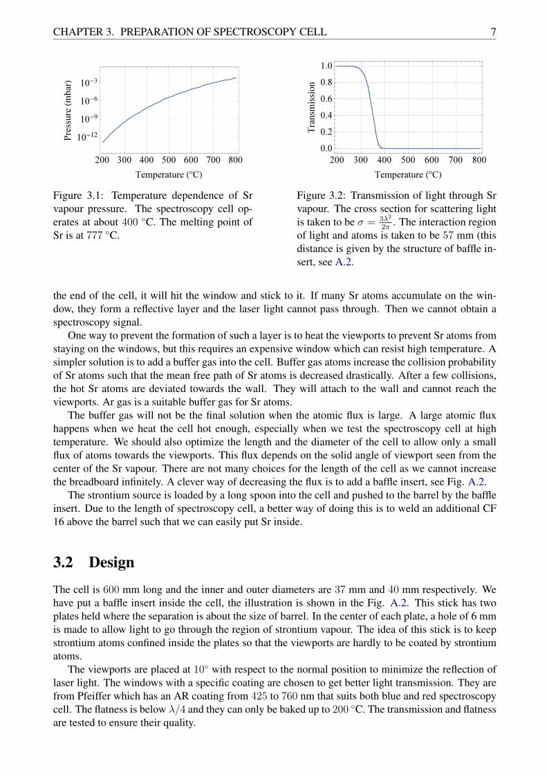
Figure 3.1: Temperature dependence of Srvapour pressure. The spectroscopy cell op-erates at about 400 C. The melting point ofSr is at 777 C.

Figure 3.2: Transmission of light through Srvapour. The cross section for scattering lightis taken to be σ = 3λ2

2π. The interaction region

of light and atoms is taken to be 57 mm (thisdistance is given by the structure of baffle in-sert, see A.2.

the end of the cell, it will hit the window and stick to it. If many Sr atoms accumulate on the win-dow, they form a reflective layer and the laser light cannot pass through. Then we cannot obtain aspectroscopy signal.

One way to prevent the formation of such a layer is to heat the viewports to prevent Sr atoms fromstaying on the windows, but this requires an expensive window which can resist high temperature. Asimpler solution is to add a buffer gas into the cell. Buffer gas atoms increase the collision probabilityof Sr atoms such that the mean free path of Sr atoms is decreased drastically. After a few collisions,the hot Sr atoms are deviated towards the wall. They will attach to the wall and cannot reach theviewports. Ar gas is a suitable buffer gas for Sr atoms.

The buffer gas will not be the final solution when the atomic flux is large. A large atomic fluxhappens when we heat the cell hot enough, especially when we test the spectroscopy cell at hightemperature. We should also optimize the length and the diameter of the cell to allow only a smallflux of atoms towards the viewports. This flux depends on the solid angle of viewport seen from thecenter of the Sr vapour. There are not many choices for the length of the cell as we cannot increasethe breadboard infinitely. A clever way of decreasing the flux is to add a baffle insert, see Fig. A.2.

The strontium source is loaded by a long spoon into the cell and pushed to the barrel by the baffleinsert. Due to the length of spectroscopy cell, a better way of doing this is to weld an additional CF16 above the barrel such that we can easily put Sr inside.

3.2 DesignThe cell is 600 mm long and the inner and outer diameters are 37 mm and 40 mm respectively. Wehave put a baffle insert inside the cell, the illustration is shown in the Fig. A.2. This stick has twoplates held where the separation is about the size of barrel. In the center of each plate, a hole of 6 mmis made to allow light to go through the region of strontium vapour. The idea of this stick is to keepstrontium atoms confined inside the plates so that the viewports are hardly to be coated by strontiumatoms.

The viewports are placed at 10 with respect to the normal position to minimize the reflection oflaser light. The windows with a specific coating are chosen to get better light transmission. They arefrom Pfeiffer which has an AR coating from 425 to 760 nm that suits both blue and red spectroscopycell. The flatness is below λ/4 and they can only be baked up to 200 C. The transmission and flatnessare tested to ensure their quality.

8 3.3. PREPARATION PROCEDURE

The cell is made from stainless steel and we have tested its quality by heating to 900 C. Therewas no break or any slit on the cell, the vacuum quality is maintained.

The illustration of the spectroscopy cell is shown in appendix A.

3.3 Preparation procedureThe baking procedure is necessary for good vacuum conditions. The tube is wrapped with heatingwire and glass fiber in order to heat homogeneously. The stainless steel absorbs water vapour and thebaking procedure accelerates the outgassing. The gas is then pumped out during baking. More detailsabout vacuum technique can be found in Ref. [24]

The cell is pre-baked without viewports. We wrap a heating wire around the tube homogeneously,then add glass fiber and aluminium foils to heat the tube to a temperature about 450 C for tens ofhours. The viewports should not be heated to a temperature higher than 200 C, so they are not usedin the pre-baking stage.

After the pre-baking, we put the cell into a plastic glove bag with Argon gas filled in. We changetwo viewports and break the ampoule of strontium inside of the bag. Strontium is loaded into the cellby a spoon and pushed to the barrel by the baffle insert. We need to make sure that there is no residualair as strontium interacts strongly with oxygen and becomes a chalk like powder which can no longerbe used in further experiment.

About 5 g of Strontium is loaded into the barrel of the cell. It can be used for few years withoutopening the cell. We can monitor the cell by using the pressure gauge and by adding buffer gas. Thepressure gauge is PCR 280 from Pfeiffer which is a combination of a diaphragm capacitive gauge anda Pirani gauge. It can measure the pressure from 5× 10−5 to 1500 hPa (hectopascal). The buffer gasshould be added during pumping for a reasonable time to eliminate any residual gas. A valve is usedto control the flow of Argon gas to attain the desired equilibrium pressure.

After adding two viewports and a pressure gauge, we re-bake our cell slowly to 200 C as thesenew elements may cause a bad vacuum condition in the cell. This baking stage takes about two days.

We can also test the sealing quality of the cell with a helium leak detector. We put Helium gas atevery CF connection and measure the Helium pressure inside the cell.

Finally, we take off the heating wire and use a heating clamp only around the barrel. Two copperblocks are added where water cooling is used. The heating region is covered again by glass fiber sheetand aluminium foil.

Chapter 4

Modulation transfer spectroscopy

Modulation transfer spectroscopy is a pump-probe scheme where we send a saturated pump beam(s0 > 1) through the strontium vapour and a weak probe beam in the opposite direction. It is asaturated absorption spectroscopy and it has a signal resolution which is close to the natural linewidth.

It can achieve a steep signal for frequency discrimination to lock the laser frequency. The capturerange is typically a few times the natural linewidth hence it is usually below 100 MHz. Modulationtransfer spectroscopy has several advantages over other techniques: it has a zero background signal,the zero crossing is centered on atomic transition and the closed atomic transitions dominate thesignals. Frequency modulation spectroscopy usually has a sloping background where an additionaldemodulation is required and it also gives a open transition signal which is not suitable for laserlocking in closely spaced spectrum [25].

We will discuss the light absorption of atoms to explain why we need this spectroscopy.

4.1 Absorption coefficientAccording to the Doppler effect, the moving atoms see different frequencies of the laser beam. In athermal gas, the atoms can be classified into different velocity classes. The frequency seen by eachclass is given by ω = ωl − ~k · ~v where ωl is the laser frequency, ~k = 2π

λk (where λ is the laser

wavelength and k is the unit vector along the laser beam propagating direction) and ~v is the velocityof atoms.

The laser light can be absorbed by the atoms in the velocity class satisfying ω0 = ωl − ~k · ~v.The velocity distribution of atoms obeys Maxwell-Boltzmann statistics which has a Gaussian shape.Hence, the absorption linewidth will not be Lorentzian but will be broadened to a Gaussian. This iscalled the Doppler broadening and the FWHM is given by [26]

∆ωD ≈ 1.7u

cω0

where u =√

2kBT/m is the most probable speed for atoms. This can be about GHz which istoo large in comparison to the natural linewidth. We need a spectroscopy technique with linewidthcomparable to the natural linewidth.

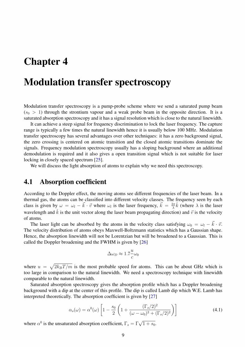
Saturated absorption spectroscopy gives the absorption profile which has a Doppler broadeningbackground with a dip at the center of this profile. The dip is called Lamb dip which W.E. Lamb hasinterpreted theoretically. The absorption coefficient is given by [27]

αs(ω) = α0(ω)

[1− s0

2

(1 +

(Γs/2)2

(ω − ω0)2 + (Γs/2)2

)](4.1)

where α0 is the unsaturated absorption coefficient, Γs = Γ√

1 + s0.

9

10 4.2. BASIC CALCULATION OF ERROR SIGNAL

The experimental signal of the Lamb dip will be presented later. We will calculate the error signalin the next section.

4.2 Basic calculation of error signalIn the modulation transfer spectroscopy, the intense pump beam is propagating through an electro-optic modulator (EOM, details can be found in appendix B) to get two sidebands. Consider the singlefrequency pump beam E = E0 sin(ω0t) and the driven frequency of the EOM is ωm. An additionaltime-dependent phase term is added to the pump beam

E = E0 sin(ω0t+m sinωmt)

where m is the modulation index given by the ratio of the driven voltage V and the half-wave voltageVπ, m = V

Vπ. ωm is called the modulation frequency. See appendix B.

By using Bessel functions Jn(x), we expand the above expression to get a beam which has acarrier term and two sidebands terms as

E = E0 sin(ω0t+m sinωmt)

= E0[Σ∞n=0Jn(m) sin(ω0 + nωm)t+ Σ∞n=1(−1)nJn(m) sin(ω0 − nωm)t

≈ E0[sinω0t+m

2sin(ω0 + ωm)t− m

2sin(ω0 − ωm)t]

=1

2E0

−m

2exp[i(ω0 − ωm)t] + exp(iω0t) +

m

2exp[i(ω0 + ωm)t]

+ c.c

Where the last two lines are valid for m 1 and we have two sidebands oscillating at ω ± ωm. Thisis an ideal case as the absorption of light is not considered. In the real case, the intensity of light willdecrease after passing through the EOM. After the two sidebands are generated, the pump beam ispassing through the area of atomic vapour.

A probe field E = Ep sin(ω0t) oscillates at the frequency ω0. It propagates through the atomicvapour in the opposite direction of the pump beam. These two beams interact in a nonlinear waysuch that a four wave mixing process occurs between one sideband and the carrier of the pump beamand the probe beam[25]. The new field beats with the probe beam creating a new signal at sidebandfrequency ωm. According to [28, 29, 30], the lineshape of the beat signal for two sidebands is givenby

S(ωm) =C√

Γ2 + ω2m

J0(m)J1(m)[(L−1 − L− 12

+ L 12− L−1) cosωmt

+ (D1 −D 12−D− 1

2+D−1) sinωmt]

(4.2)

where

Ln =Γ2

Γ2 + (δ − nωm)2

is the Lorentzian resonance function and

Dn =Γ(δ − nωm)

Γ2 + (δ − nωm)2

Γ is the natural linewidth and δ is the detuning. C is a constant number.Using heterodyne detection, the absorption signal or the dispersion signal can be detected by

changing the phase of the local oscillator. We can plot the dispersion and absorption lineshapes by

CHAPTER 4. MODULATION TRANSFER SPECTROSCOPY 11

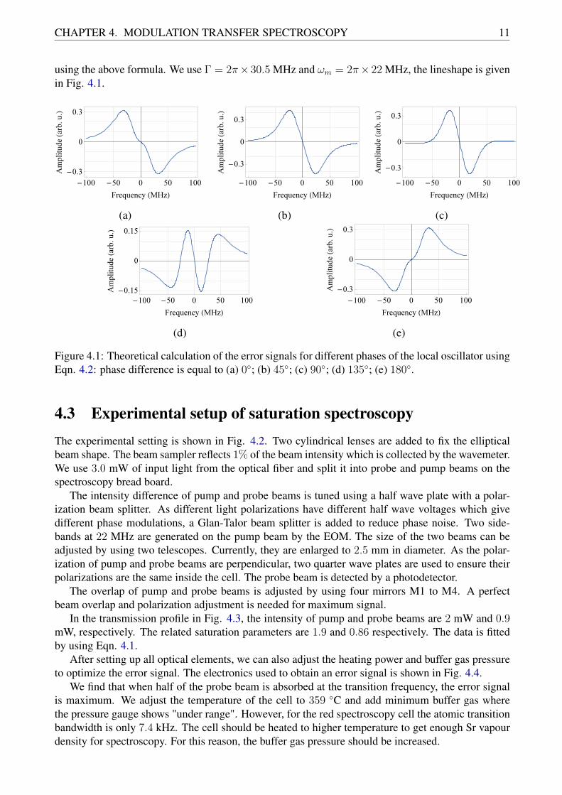
using the above formula. We use Γ = 2π× 30.5 MHz and ωm = 2π× 22 MHz, the lineshape is givenin Fig. 4.1.

(a) (b) (c)

(d) (e)

Figure 4.1: Theoretical calculation of the error signals for different phases of the local oscillator usingEqn. 4.2: phase difference is equal to (a) 0; (b) 45; (c) 90; (d) 135; (e) 180.

4.3 Experimental setup of saturation spectroscopyThe experimental setting is shown in Fig. 4.2. Two cylindrical lenses are added to fix the ellipticalbeam shape. The beam sampler reflects 1% of the beam intensity which is collected by the wavemeter.We use 3.0 mW of input light from the optical fiber and split it into probe and pump beams on thespectroscopy bread board.

The intensity difference of pump and probe beams is tuned using a half wave plate with a polar-ization beam splitter. As different light polarizations have different half wave voltages which givedifferent phase modulations, a Glan-Talor beam splitter is added to reduce phase noise. Two side-bands at 22 MHz are generated on the pump beam by the EOM. The size of the two beams can beadjusted by using two telescopes. Currently, they are enlarged to 2.5 mm in diameter. As the polar-ization of pump and probe beams are perpendicular, two quarter wave plates are used to ensure theirpolarizations are the same inside the cell. The probe beam is detected by a photodetector.

The overlap of pump and probe beams is adjusted by using four mirrors M1 to M4. A perfectbeam overlap and polarization adjustment is needed for maximum signal.

In the transmission profile in Fig. 4.3, the intensity of pump and probe beams are 2 mW and 0.9mW, respectively. The related saturation parameters are 1.9 and 0.86 respectively. The data is fittedby using Eqn. 4.1.

After setting up all optical elements, we can also adjust the heating power and buffer gas pressureto optimize the error signal. The electronics used to obtain an error signal is shown in Fig. 4.4.

We find that when half of the probe beam is absorbed at the transition frequency, the error signalis maximum. We adjust the temperature of the cell to 359 C and add minimum buffer gas wherethe pressure gauge shows "under range". However, for the red spectroscopy cell the atomic transitionbandwidth is only 7.4 kHz. The cell should be heated to higher temperature to get enough Sr vapourdensity for spectroscopy. For this reason, the buffer gas pressure should be increased.

12 4.3. EXPERIMENTAL SETUP OF SATURATION SPECTROSCOPY

Laser

Cylindrical

Lenses

(a)

Collimation

Lenses 2 2

Glan-Taylor

Polarizer

EOM Telescope2

Telescope

4 4

M1

M2

PD

Spectroscopy Cell

M3

M4

(b)

Figure 4.2: (a) Optical setup for the blue master laser. The spectroscopy setup shown in (b) is opti-mized to only use 3 mW light out of fiber. Components are taken from Inkscape ComponentLibrary.

Figure 4.3: The transmission signal and fit function given by Eqn. 4.1. The solid red curve is the datawhich is fitted by the dashed blue curve. The temperature of the spectroscopy cell is 359 C (Thistemperature is measured at the bottom of the barrel). The beam diameter is 2.5 mm and the intensityof pump and probe beams are 2 mW and 0.9 mW, respectively.

CHAPTER 4. MODULATION TRANSFER SPECTROSCOPY 13

Function

Generator

CH 1

CH 2

Phase

Delay

Line l.o.

EOM PD

r.f.i.f.

Low-Pass

Filter

PID SC 100

Offset V

VoltageSummer

PZT+

Spectrum

Analyzer

Spectroscopy

Cell

Figure 4.4: The electronics for negative feedback frequency locking. CH1 and CH2 are two outputchannels of a function generator. The phase of the local oscillator (l.o.) can be changed by adjustingthe different phases on the function generator or by changing the cable length. The photodiode (PD)has two ports, one is the DC port, which is sent to oscilloscope for transmission signal, the other is theAC port, which is sent to the radio frequency (r.f.) part of a frequency mixer. A proportional-integral-derivative controller (PID) and a scan controller (SC) are used to control the piezoelectric transducer(PZT) in the laser head.

(a) (b) (c)

(d) (e)

Figure 4.5: Error signal for different phases. The scales of these signals in 20 mV per box in thevertical axis and 10 ms per box in the horizontal axis. These data are taken at higher input beam in-tensity for better illustration. For different phases of the local oscillator, we observe: phase differenceis equal to (a) 0; (b) 45; (c) 90; (d) 135; (e) 180. The error signals show good correspondence totheoretical calculation in Fig. 4.1.

14 4.3. EXPERIMENTAL SETUP OF SATURATION SPECTROSCOPY

The error signal is also strongly influenced by the phase difference of the radio frequency andlocal oscillator signals. We fix the phase of the radio frequency signal and tune the phase of the localoscillator by directly adjusting the phase of the function generator or by changing the phase delayline. Here we show the phase dependences of the error signal in Fig. 4.5.

We should choose a phase of local oscillator to make an error signal which has a zero crossing attransition frequency. Besides, its magnitude should be as large as possible to avoid unlock by noise.

In Fig. 4.5, we can also observe a second error signal. This error signal is located at about 120MHz below the first error signal. The isotope shift of 86Sr is −124.8 MHz and its the second mostabundant isotope. Hence 86Sr gives the second error signal.

Chapter 5

Laser frequency stabilization

In this section, we will briefly introduce a basic theory to study the dynamic properties of the laserstabilization system and then talk about how to realize a reliable laser locking. For readers who areinterested in these topics, [31] is a good reference.

5.1 Linear control system

The general control system can be split into two parts. One is a control system which is calledcontroller and the other is a plant which represents the process being controlled. The control loop canform a negative feedback such that when an error of output is detected, a response signal is generatedto have an opposite sign of initial out to correct it back to the set value.

Consider the gain function of the controller and plant as gc(t) and gp(t), respectively. The initialinput vi(t) is amplified to the convolution of gp and gc in the closed negative feedback loop by

vo(t) =

∫ t

−∞g(t− t′) (vi(t

′)− vo(t′)) dt′

where g(t) is the total gain given by

g(t) =

∫ t

−∞gp(t− t′)gc(t′)dt′

A useful way to consider the above equations is to use the Laplace transformation. For any ordi-nary function f(t), the Laplace transformation is

F (s) = L[f ] =

∫ ∞0

e−stf(t)dt

If we apply the Laplace transformation to g(t), the convolution transforms to a simple product

G(s) = Gp(s)Gc(s)

We can use the block diagram to show the relation of different blocks, where a block representsthe principle function of a system part. The relation between different blocks is indicated by arrowsand the summer with plus and minus sign at the inputs. The closed negative feedback loop has theblock diagram given in Fig. 5.1

15

16 5.2. FREQUENCY LOCKING PROCEDURE

p c+

-

i oV Vs s

Figure 5.1: The block diagram of a negative feedback loop, the overall transfer function is G(s) =Gp(s)Gc(s). The + and − signs indicate negative feedback of the control loop.

From this diagram, the Laplace transformed input and output voltages are related by

Vo(s) = G(s) (Vi(s)− Vo(s))

The transfer function H(s) is

H(s) =Vo(s)

Vi(s)=

G(s)

1 +G(s)

For laser frequency stabilization, a frequency discriminant will generate a response signal whenlaser frequency does not equal to the set frequency. This response signal is amplified by a loop filterto control the piezoelectric transducer or driving current of the laser.

Assume the laser frequency f depends linearly on the amplified response signal f = f1 + κVc. Vcis the voltage given by the control loop. It is always a reasonable assumption in the range of transitionlinewidth. This dependence allows us to directly consider the transfer function between the input andoutput frequencies.

In the control part, the output frequency f is compared to f0 which is the atomic transition fre-quency at zero crossing of the error signal. There is one difference between the block diagram 5.1and our system. The feedback signal is proportional to the frequency difference ∆f = f − f0.

Following the block diagram and the Ref. [31], the loop equation can be written by

F (s) = F1(s)−G(s)× (F (s)− F0(s))

then

F (s) = F1(s)1

1 +G(s)+ F0(s)

G(s)

1 +G(s)

where F (s), F1(s) and F0(s) are the Laplace transforms of f , f1 and f0 respectively.We can characterize the frequency noise by considering the laser frequency jitter ∆F1 and the

reference frequency noise ∆F0. Using above formula, we have

∆F = ∆F11

1 +G(s)+ ∆F0

G(s)

1 +G(s)

In the regime whereG(s) 1, ∆F1 is suppressed and only noise from the frequency discriminantis important. In our case, this noise comes from the error signal zero crossing fluctuation.

5.2 Frequency locking procedureThe basic loop filters take the integral, differential or proportional of the error signal. Their combina-tions form the simplest controller. In our case, we use the Toptica PID 110 in combination with SC100. The PID controller has a transfer function [31]

GPID(s) = Kp +Ki1

s+Kds

CHAPTER 5. LASER FREQUENCY STABILIZATION 17

The laser head with all the electronic equipment form the experiment part are treated as a black boxbecause of no available analytic expression of the transfer function. We tune the PID to generate afast responding overall transfer function.

In order to get good laser stabilization, we need to adjust the temperature and current of the laserto avoid mode hoping. After choosing an appropriate running condition, we can start to lock the laserfrequency in the following steps:

1. Before locking the laser frequency, we should set the laser frequency to the atomic transitionfrequency. A simple way of doing that is to use an offset voltage and a voltage summer to adjustthe voltage on the PZT, see Fig. 4.4.

2. Turn up the scan amplitude to show the error signal on the oscilloscope, like Fig. 4.5 (a).

3. Choose the correct direction of PID action according to Fig. 5.2.

4. Adjust the set point of the PID controller to put error signal at zero crossing, then turn downscan amplitude.

5. Keep the PID controller off and set the P, I and D trimpots farthest to the left where they haveminimum gain. Set the PID gain potentiometer to an intermediate value.

6. Turn on the PID controller and increase the I trimpot to get an initial lock. We can see an errorsignal similar to Fig. 5.3 (a). Decrease I to get an error signal similar to Fig. 5.3 (c).

7. Increase the P and D trimpots until oscillation, similarly as in Fig. 5.3 (d). Decrease P and D toget rid of the oscillation.

8. Check the locking stability by measuring the error signal noise with the spectrum analyzer.

5.3 Characterization of locking stabilityTo measure the stability of an oscillator, there are two basic ways. One is in the time domain, wemeasure the mean of the output signal during fixed period to determine the signal variance. The otheris in the frequency domain, we use the power spectrum of output fluctuation to calculate the frequencynoise.

For a laser, it is usually hard to count the radiation circle precisely so usually people study the laserstability in frequency domain. In our experiment, we can access the error signal spectrum density witha Stanford sr 760 fft spectrum analyzer.

Assuming laser light has only phase noise φ(t) such that its amplitude E0 is constant. The laserlight can be described by [31]

E(t) = E0 sin(2πf0t+ φ(t))

where f0 is the laser’s frequency without noise. The instantaneous frequency is defined by

f(t) = f0 +1

2π

dφ

dt

The frequency fluctuation is given by

∆f(t) = f(t)− f0 =1

2π

dφ

dt(5.1)

18 5.3. CHARACTERIZATION OF LOCKING STABILITY

Figure 5.2: The scales of these signals are 10 mV per box in the vertical axis and 50 ms per box inthe horizontal axis. The top signal is the error signal and the bottom signal is the PZT scan voltage.The laser frequency decreases when the scan voltage increases, which can be confirmed as the isotopeerror signal appears at a lower PZT voltage. The relation between scan voltage and laser frequencydetermines the required gain sign of the servo loop.

(a) The laser frequency is locked. The P andD trimpots are turned to zero and the errorsignal is slightly above the red line.

(b) The laser frequency is locked. The P andD trimpots are turned to zero and the errorsignal is slightly below the red line.

(c) The laser frequency is locked. The P andD trimpots are turned to zero and the errorsignal is on the red line.

(d) The laser frequency is locked. Startingfrom the settings in panel (c), the P and Dtrimpots are increased to observe oscillation.

Figure 5.3: The scales of these signals are 10 mV per box in the vertical axis and 50 ms per box inthe horizontal axis. The panels show the error signal from the monitor output of the PID controller.

CHAPTER 5. LASER FREQUENCY STABILIZATION 19

By Wiener-Khintchine theorem, the power spectrum of phase noise Sφ(f) is the Fourier transformof its autocorrelation function Rφ(t)

Rφ(t) = limT→∞

1

T

∫ T/2

−T/2φ(t+ t′)φ(t)dt′

Sφ(ω) =1

2π

∫ ∞−∞

Rφ(t)eiωtdt

However, what we are interested in is not phase noise spectrum density but the frequency noisespectrum density. According to Eqn. 5.1,

Sφ(ω) = ω2Sφ(ω)

hence〈φ2〉 = Rφ(0) =

∫ ∞−∞

Sφ(ω)dω

As the measurement from spectrum analyzer gives spectral density in positive frequencies, themean square frequency deviation 〈(∆f)2〉 is given by the spectral density of frequency fluctuationsS∆f (f)

〈(∆f)2〉 =

∫ ∞0

S∆f (f)df

where the one-sided spectral density is used.Typically, the free running diode laser has a linewidth of a few MHz. Frequency locking reduces

this linewidth smaller than the atomic transition linewidth. In our experiment, the linewidth of thelaser is measured by the density power spectrum of the error signal obtained from the spectroscopybreadboard. The error signal amplitude is linearly dependent on the detuning frequency in the rangeof the natural linewidth.

From Fig. 4.5 (a), we can measure the proportionality constant between the error signal amplitudeand frequency. We measure the density power spectrum of the error signal when laser is runningfreely and when the laser is locked. The measurements are shown in Fig. 5.4.

Figure 5.4: (a) Power spectrum density (PSD in the figure, unit in µVrms/√Hz) of the error signal,

(b) PSD is zoomed in. The solid red curve is for the free running laser close to the locking frequencyand the dashed blue curve is for the locked laser.

The noise is reduced after the locking procedure. From this in-loop measurement, we cannotconclude that the laser linewidth is reduced. However, by integrating the error signal PSD, we canestimate that the servo reduces the frequency excursions by a factor of 3 approximately. The maincontribution of noise after locking comes from low frequencies. They are harmonics of 50 Hz lab ACsupplies. The low frequency noise will be reduced to get a narrower linewidth.

Chapter 6

Conclusion and outlook

We built a system to stabilize the frequency of a Toptica diode laser system to a saturated absorptionspectroscopy. The laser light is split into a pump beam and a probe beam. The intense pump beamis modulated by an EOM and then goes through Sr vapour to saturate atoms in excited state whilethe weak probe beam propagates in the opposite direction. The transmission signal from probe beamshows a Lamb dip in a Doppler broaden transmission profile. This is a basic saturation spectroscopyscheme. The modulation frequency in pump beam is transferred to the probe beam via four wavemixing process.

The transmitted probe signal is analyzed by electronic devices to give an error signal which has azero crossing at the atomic transition frequency. This error signal is used in a PID controller to lockthe diode laser frequency. The in-loop error signal is examined with a 100 kHz Fourier transformationspectrum analyzer to ensure the good locking quality.

After locking the blue laser to the Sr transition, we will use it as the reference further blue diodeslasers for power amplification. We designed a diode laser mount compatible with injection locking,shown in appendix C.

In the blue laser system, acousto-tptical modulators (AOMs) will be added to shift frequency fortransverse cooling, the Zeeman slower and the MOT. A similar setup will be built for the red lasersystem with an additional optical cavity to reduce the laser linewidth below 7.4 kHz. We are in theprocess of designing the vacuum system for cooling and trapping of Sr based on these new lasersystems.

Many proposals will be possible to realize with strontium experiments. Recently, there was aproposal about a toy model in QCD which can be realized in strontium optical lattice [32]. Thefermionic strontium atoms have nuclear spin I = 9/2 representing the SU(N ) spins model withN ≤ 2I + 1. Among these SU(N ) models, certain effective low-energy (2+1) dimensional spinladder models of SU(N ) can produce the (1+1) dimensional CP(N −1) model under the dimensionalreduction where the continuous limit is taken. Another proposal [33] discussed the possibility to studylattice gauge theories in the strontium optical lattice. These proposals show a lot of exciting physicsin quantum simulation of particle physics via the strontium optical lattice.

20

Appendix A

Spectroscopy cell design

The spectroscopy cell we use was originally designed by A. Mayer. For the next version of thecell, we would like to add a CF 16 flange on the top of the barrel such that it is convenient to loadstrontium into the barrel. The cell which is used in the blue laser spectroscopy is shown in the Fig.A.1. To prevent coating the viewports we added two baffles around the Sr reservoir (see Fig. A.2).Additionally, the cell is water cooled.

(a)

10°

6,89

33,75

12,7012,70

(b)

Figure A.1: (a) Blue laser spectroscopy cell and (b) windows. The window has a 10 angle with thetube. This angle should be designed to minimize the reflection of laser light.

1,50 1,50

6,00

Ø

6,00

Ø

6,00

Ø

n6,00

n4,00

Figure A.2: The baffle insert is put into the cell, the total length is 490mm and the distance betweentwo baffles are 57 mm. The hole in the center of baffle allows light go through Sr vapour while keep Sratoms stay in this region as the aperture of the hole is 6 mm in comparison with 40 mm cell diameter.This small aperture reduce the flux of Sr towards viewport and prevent windows from Sr coating.

21

Appendix B

Homebuilt Electro-optic modulator

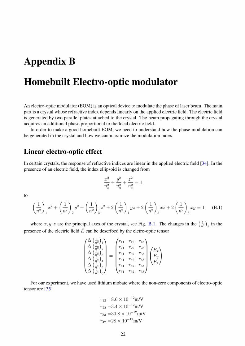
An electro-optic modulator (EOM) is an optical device to modulate the phase of laser beam. The mainpart is a crystal whose refractive index depends linearly on the applied electric field. The electric fieldis generated by two parallel plates attached to the crystal. The beam propagating through the crystalacquires an additional phase proportional to the local electric field.

In order to make a good homebuilt EOM, we need to understand how the phase modulation canbe generated in the crystal and how we can maximize the modulation index.

Linear electro-optic effectIn certain crystals, the response of refractive indices are linear in the applied electric field [34]. In thepresence of an electric field, the index ellipsoid is changed from

x2

n2x

+y2

n2y

+z2

n2z

= 1

to (1

n2

)1

x2 +

(1

n2

)2

y2 +

(1

n2

)3

z2 + 2

(1

n2

)4

yz + 2

(1

n2

)5

xz + 2

(1

n2

)6

xy = 1 (B.1)

where x, y, z are the principal axes of the crystal, see Fig. B.1. The changes in the(

1n2

)k

in thepresence of the electric field ~E can be described by the elctro-optic tensor

∆(

1n2

)1

∆(

1n2

)2

∆(

1n2

)3

∆(

1n2

)4

∆(

1n2

)5

∆(

1n2

)6

=

r11 r12 r13

r21 r22 r23

r31 r32 r33

r41 r42 r43

r51 r52 r53

r61 r62 r63

ExEyEz

For our experiment, we have used lithium niobate where the non-zero components of electro-optictensor are [35]

r13 =8.6× 10−12m/Vr22 =3.4× 10−12m/Vr33 =30.8× 10−12m/Vr42 =28× 10−12m/V

22

APPENDIX B. HOMEBUILT ELECTRO-OPTIC MODULATOR 23

x axis

y axis

z axis

VAC

voltage

W

L

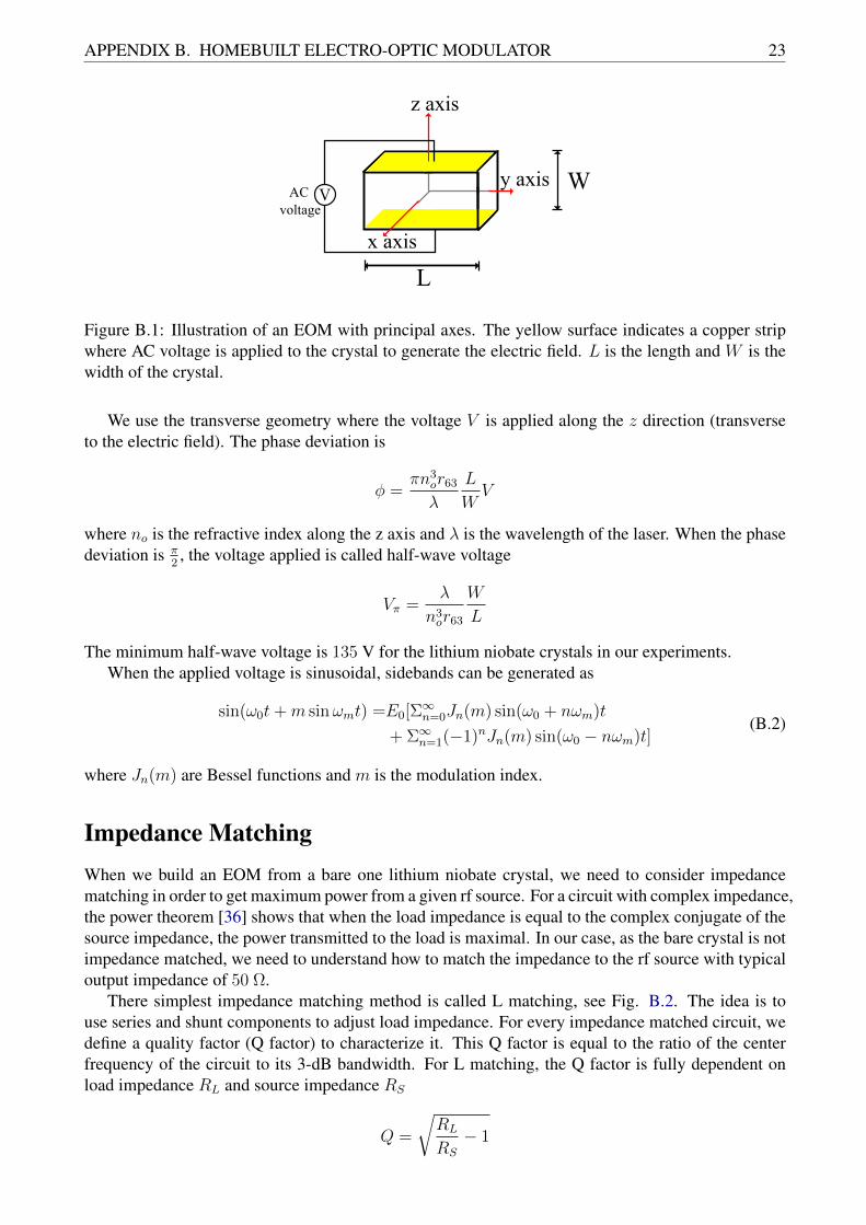
Figure B.1: Illustration of an EOM with principal axes. The yellow surface indicates a copper stripwhere AC voltage is applied to the crystal to generate the electric field. L is the length and W is thewidth of the crystal.

We use the transverse geometry where the voltage V is applied along the z direction (transverseto the electric field). The phase deviation is

φ =πn3

or63

λ

L

WV

where no is the refractive index along the z axis and λ is the wavelength of the laser. When the phasedeviation is π

2, the voltage applied is called half-wave voltage

Vπ =λ

n3or63

W

L

The minimum half-wave voltage is 135 V for the lithium niobate crystals in our experiments.When the applied voltage is sinusoidal, sidebands can be generated as

sin(ω0t+m sinωmt) =E0[Σ∞n=0Jn(m) sin(ω0 + nωm)t

+ Σ∞n=1(−1)nJn(m) sin(ω0 − nωm)t](B.2)

where Jn(m) are Bessel functions and m is the modulation index.

Impedance MatchingWhen we build an EOM from a bare one lithium niobate crystal, we need to consider impedancematching in order to get maximum power from a given rf source. For a circuit with complex impedance,the power theorem [36] shows that when the load impedance is equal to the complex conjugate of thesource impedance, the power transmitted to the load is maximal. In our case, as the bare crystal is notimpedance matched, we need to understand how to match the impedance to the rf source with typicaloutput impedance of 50 Ω.

There simplest impedance matching method is called L matching, see Fig. B.2. The idea is touse series and shunt components to adjust load impedance. For every impedance matched circuit, wedefine a quality factor (Q factor) to characterize it. This Q factor is equal to the ratio of the centerfrequency of the circuit to its 3-dB bandwidth. For L matching, the Q factor is fully dependent onload impedance RL and source impedance RS

Q =

√RL

RS

− 1

24

In order to get a high Q, we need to use three elements circuits, π matching or T matching. Thesetwo circuits can be understood by a combination of two L matching circuits.

X1

RS

X2 RL

(a)

X1

X2RS

X3 RL

(b)

X1

RS

X2 RL

X3

(c)

Figure B.2: (a) L matching. (b) π matching. (c) T matching. Figure reproduced from [36]

The Smith chart was created in the second world war to help radio frequency engineers to calculatecomplex impedance and reflection coefficients Γ. For a load impedance ZL and a source impedanceZS , the reflection coefficient is given by

Γ =ZS − ZLZS + ZL

In the Smith chart, all the values are normalized by the source impedance.A superposition of Smith chart and a 180 rotation of Smith chart is sometimes called YZ chart

as it shows both impedance Z and admittance Y. These charts are extremely useful and very easy tolearn for a layman to do impedance matching trials.

In our case, the capacitance of EOM crystal is specified 12.3 pF and we want to build a circuitwith resonance frequency at 22 MHz. We add two shunt capacitors and make an series inductor bycopper wire for a π matching. The complete matching circuit of our homebuilt EOM is shown in theFig. B.3.

Figure B.3: The matching circuit for the EOM. A indicates the source capacitors with a tunablecapacitance, B is the coil (inductance) and C is the load capacitor.

The approach of selecting capacitors and inductors are shown in the Fig. B.4

APPENDIX B. HOMEBUILT ELECTRO-OPTIC MODULATOR 25

RADI ALLY SCALED PARAMETERS

TOWARD LOAD —> <— TOWARD GENERATOR1.11.21.41.61.822.5345102040100

SWR1

12345681015203040

dBS1

1234571015 ATTE

N. [

dB]

1.1 1.2 1.3 1.4 1.6 1.8 2 3 4 5 10 20 S.W.

LOS

S CO

EFF

1

0 1 2 3 4 5 6 7 8 9 10 12 14 20 30

RTN. LOSS [dB]

0.010.050.10.20.30.40.50.60.70.80.91

RFL. COEFF, P 0

0.1 0.2 0.4 0.6 0.8 1 1.5 2 3 4 5 6 10 15 RFL.

LOS

S [d

B]

0

1.1 1.2 1.3 1.4 1.5 1.6 1.7 1.81.9 2 2.5 3 4 5 10 S.W.

PEA

K (C

ONST

. P)

0

0.10.20.30.40.50.60.70.80.91

RFL. COEFF, E or I

0 0.99 0.95 0.9 0.8 0.7 0.6 0.5 0.4 0.3 0.2 0.1 0 TRAN

SM.

COEF

F, P

1

CENTER

1 1.1 1.2 1.3 1.4 1.5 1.6 1.7 1.8 1.9 2 TRAN

SM.

COEF

F, E

or

I

0 0.1 0.2 0.3 0.4 0.5 0.6 0.7 0.8 0.9

ORI GI N

0.1

0.1

0.2

0.2

0.2

0.3

0.3

0.4

0.4

0.4

0.5

0.5

0.5

0.6

0.6

0.6

0.7

0.7

0.7

0.8

0.8

0.8

0.9

0.9

0.9

1.0

1.0

1.0

1.2

1.2

1.2

1.4

1.4

1.4

1.6

1.6

1.6

1.8

1.8

1.8

2.0

2.0

2.0

3.0

3.0

3.0

4.0

4.0

4.0

5.0

5.0

5.0

10

10

10

20

20

20

50

50

50

0.2

0.2

0.2

0.2

0.4

0.4

0.4

0.4

0.6

0.6

0.6

0.6

0.8

0.8

0.8

0.8

1.0

1.0

1.0

1.0

0.1

0.1

0.1

0.2

0.2

0.2

0.3

0.3

0.3

0.4

0.4

0.4

0.5

0.5

0.5

0.6

0.6

0.6

0.7

0.7

0.7

0.8

0.8

0.8

0.9

0.9

0.9

1.0

1.0

1.0

1.2

1.2

1.2

1.4

1.4

1.4

1.6

1.6

1.6

1.8

1.8

1.8

2.0

2.0

2.0

3.0

3.0

3.0

4.0

4.0

4.0

5.0

5.0

5.0

10

10

20

20

20

50

50

50

0.2

0.2

0.2

0.2

0.4

0.4

0.4

0.4

0.6

0.6

0.6

0.6

0.8

0.8

0.8

0.8

1.0

1.0

1.0

1.0

20

-20

30

-30

40-40

50

-50

60

-60

70

-70

80

-80

90

-90

100

-100

110

-110

120

-120

130

-130

140

-140

150

-150

160

-160

170

-170

180

±

90

-90

85

-85

80

-80

75

-75

70

-70

65

-65

60

-60

55

-55

50-50

45

-45

40

-40

35

-35

30

-30

25

-25

20

-20

15

-15

10

-10

0.04

0.04

0.05

0.05

0.06

0.06

0.07

0.07

0.08

0.08

0.09

0.09

0.1

0.1

0.11

0.11

0.12

0.12

0.13

0.13

0.14

0.14

0.15

0.15

0.16

0.16

0.17

0.17

0.18

0.18

0.19

0.19

0.2

0.2

0.21

0.21

0.22

0.22

0.23

0.23

0.24

0.24

0.25

0.25

0.26

0.26

0.27

0.27

0.28

0.28

0.29

0.29

0.3

0.3

0.31

0.31

0.32

0.32

0.33

0.33

0.34

0.34

0.35

0.35

0.36

0.36

0.37

0.37

0.38

0.38

0.39

0.39

0.4

0.4

0.41

0.41

0.42

0.42

0.43

0.43

0.44

0.44

0.45

0.45

0.46

0.46

0.47

0.47

0.48

0.48

0.49

0.49

00

AN

GLE

OF

TRA

NSM

ISS

ON

CO

EFFIC

IEN

TIN

DEG

REES

AN

GLE

OF

REFLECTIO

NC

OEFF

CIE

NT

IND

EG

REES

—>

WA

VELEN

GTH

STO

WA

RD

GEN

ERA

TO

R—>

<—

WA

VELEN

GTH

STO

WA

RD

LO

AD<—

IND

UCTIV

EREACTAN

CE

COM

PONEN

T(+jX/Z

o),O

RCA

PACIT

IVE SU

SCEPTANCE (+

jB/Yo)

EACTANCECOM

PONEN

T(-

jX/Zo),O

RIN

DUCTIV

ESU

SCEPTA

NCE(-jB

Yo)

RESI STANCE COMPONENT (R/Zo) , OR CONDUCTANCE COMPONENT (G/Yo)

NORMALIZED IMPEDANCE AND ADMITTANCE COORDINATES

RVE

I TI CAPAC

S L Z =2.1

Y =0.48L

L

A

Shunt

capacitor

+j 3.3

Z =0.04-j0.3

Y =0.48+j3.3A

A

RADI ALLY SCALED PARAMETERS

TOWARD LOAD —> <— TOWARD GENERATOR1.11.21.41.61.822.5345102040100

SWR1

12345681015203040

dBS1

1234571015 ATTE

N. [

dB]

1.1 1.2 1.3 1.4 1.6 1.8 2 3 4 5 10 20 S.W.

LOS

S CO

EFF

1

0 1 2 3 4 5 6 7 8 9 10 12 14 20 30

RTN. LOSS [dB]

0.010.050.10.20.30.40.50.60.70.80.91

RFL. COEFF, P 0

0.1 0.2 0.4 0.6 0.8 1 1.5 2 3 4 5 6 10 15 RFL.

LOS

S [d

B]

0

1.1 1.2 1.3 1.4 1.5 1.6 1.7 1.81.9 2 2.5 3 4 5 10 S.W.

PEA

K (C

ONST

. P)

0

0.10.20.30.40.50.60.70.80.91

RFL. COEFF, E or I

0 0.99 0.95 0.9 0.8 0.7 0.6 0.5 0.4 0.3 0.2 0.1 0 TRAN

SM.

COEF

F, P

1

CENTER

1 1.1 1.2 1.3 1.4 1.5 1.6 1.7 1.8 1.9 2 TRAN

SM.

COEF

F, E

or

I

0 0.1 0.2 0.3 0.4 0.5 0.6 0.7 0.8 0.9

ORI GI N

0.1

0.1

0.2

0.2

0.2

0.3

0.3

0.4

0.4

0.4

0.5

0.5

0.5

0.6

0.6

0.6

0.7

0.7

0.7

0.8

0.8

0.8

0.9

0.9

0.9

1.0

1.0

1.0

1.2

1.2

1.2

1.4

1.4

1.4

1.6

1.6

1.6

1.8

1.8

1.8

2.0

2.0

2.0

3.0

3.0

3.0

4.0

4.0

4.0

5.0

5.0

5.0

10

10

10

20

20

20

50

50

50

0.2

0.2

0.2

0.2

0.4

0.4

0.4

0.4

0.6

0.6

0.6

0.6

0.8

0.8

0.8

0.8

1.0

1.0

1.0

1.0

0.1

0.1

0.1

0.2

0.2

0.2

0.3

0.3

0.3

0.4

0.4

0.4

0.5

0.5

0.5

0.6

0.6

0.6

0.7

0.7

0.7

0.8

0.8

0.8

0.9

0.9

0.9

1.0

1.0

1.0

1.2

1.2

1.2

1.4

1.4

1.4

1.6

1.6

1.6

1.8

1.8

1.8

2.0

2.0

2.0

3.0

3.0

3.0

4.0

4.0

4.0

5.0

5.0

5.0

10

10

20

20

20

50

50

50

0.2

0.2

0.2

0.2

0.4

0.4

0.4

0.4

0.6

0.6

0.6

0.6

0.8

0.8

0.8

0.8

1.0

1.0

1.0

1.0

20

-20

30

-30

40-40

50

-50

60

-60

70

-70

80

-80

90

-90

100

-100

110

-110

120

-120

130

-130

140

-140

150

-150

160

-160

170

-170

180

±

90

-90

85

-85

80

-80

75

-75

70

-70

65

-65

60

-60

55

-55

50-50

45

-45

40

-40

35

-35

30

-30

25

-25

20

-20

15

-15

10

-10

0.04

0.04

0.05

0.05

0.06

0.06

0.07

0.07

0.08

0.08

0.09

0.09

0.1

0.1

0.11

0.11

0.12

0.12

0.13

0.13

0.14

0.14

0.15

0.15

0.16

0.16

0.17

0.17

0.18

0.18

0.19

0.19

0.2

0.2

0.21

0.21

0.22

0.22

0.23

0.23

0.24

0.24

0.25

0.25

0.26

0.26

0.27

0.27

0.28

0.28

0.29

0.29

0.3

0.3

0.31

0.31

0.32

0.32

0.33

0.33

0.34

0.34

0.35

0.35

0.36

0.36

0.37

0.37

0.38

0.38

0.39

0.39

0.4

0.4

0.41

0.41

0.42

0.42

0.43

0.43

0.44

0.44

0.45

0.45

0.46

0.46

0.47

0.47

0.48

0.48

0.49

0.49

00

AN

GLE

OF

TRA

NSM

ISS

ON

CO

EFFIC

IEN

TIN

DEG

REES

AN

GLE

OF

REFLECTIO

NC

OEFF

CIE

NT

IND

EG

REES

—>

WA

VELEN

GTH

STO

WA

RD

GEN

ERA

TO

R—>

<—

WA

VELEN

GTH

STO

WA

RD

LO

AD<—

IND

UCTIV

EREACTAN

CE

COM

PONEN

T(+jX/Z

o),O

RCA

PACIT

IVE SU

SCEPTANCE (+

jB/Yo)

EACTANCECOM

PONEN

T(-

jX/Zo),O

RIN

DUCTIV

ESU

SCEPTA

NCE(-jB

Yo)

RESI STANCE COMPONENT (R/Zo) , OR CONDUCTANCE COMPONENT (G/Yo)

NORMALIZED IMPEDANCE AND ADMITTANCE COORDINATES

RVE

I TI CAPAC

A

S L

Z =0.04-j0.3

Y =0.48+j3.3A

A

B

Series

inductor

+j 0.5

Z =0.04+j0.2

Y =0.96-j4.7B

B

RADI ALLY SCALED PARAMETERS

TOWARD LOAD —> <— TOWARD GENERATOR1.11.21.41.61.822.5345102040100

SWR1

12345681015203040

dBS1

1234571015 ATTE

N. [

dB]

1.1 1.2 1.3 1.4 1.6 1.8 2 3 4 5 10 20 S.W.

LOS

S CO

EFF

1

0 1 2 3 4 5 6 7 8 9 10 12 14 20 30

RTN. LOSS [dB]

0.010.050.10.20.30.40.50.60.70.80.91

RFL. COEFF, P 0

0.1 0.2 0.4 0.6 0.8 1 1.5 2 3 4 5 6 10 15 RFL.

LOS

S [d

B]

0

1.1 1.2 1.3 1.4 1.5 1.6 1.7 1.81.9 2 2.5 3 4 5 10 S.W.

PEA

K (C

ONST

. P)

0

0.10.20.30.40.50.60.70.80.91

RFL. COEFF, E or I

0 0.99 0.95 0.9 0.8 0.7 0.6 0.5 0.4 0.3 0.2 0.1 0 TRAN

SM.

COEF

F, P

1

CENTER

1 1.1 1.2 1.3 1.4 1.5 1.6 1.7 1.8 1.9 2 TRAN

SM.

COEF

F, E

or

I

0 0.1 0.2 0.3 0.4 0.5 0.6 0.7 0.8 0.9

ORI GI N

0.1

0.1

0.2

0.2

0.2

0.3

0.3

0.4

0.4

0.4

0.5

0.5

0.5

0.6

0.6

0.6

0.7

0.7

0.7

0.8

0.8

0.8

0.9

0.9

0.9

1.0

1.0

1.0

1.2

1.2

1.2

1.4

1.4

1.4

1.6

1.6

1.6

1.8

1.8

1.8

2.0

2.0

2.0

3.0

3.0

3.0

4.0

4.0

4.0

5.0

5.0

5.0

10

10

10

20

20

20

50

50

50

0.2

0.2

0.2

0.2

0.4

0.4

0.4

0.4

0.6

0.6

0.6

0.6

0.8

0.8

0.8

0.8

1.0

1.01.0

1.0

0.1

0.1

0.1

0.2

0.2

0.2

0.3

0.3

0.3

0.4

0.4

0.4

0.5

0.5

0.5

0.6

0.6

0.6

0.7

0.7

0.7

0.8

0.8

0.8

0.9

0.9

0.9

1.0

1.0

1.0

1.2

1.2

1.2

1.4

1.4

1.4

1.6

1.6

1.6

1.8

1.8

1.8

2.0

2.0

2.0

3.0

3.0

3.0

4.0

4.0

4.0

5.0

5.0

5.0

10

10

20

20

20

50

50

50

0.2

0.2

0.2

0.2

0.4

0.4

0.4

0.4

0.6

0.6

0.6

0.6

0.8

0.8

0.8

0.8

1.0

1.0

1.0

1.0

20

-20

30

-30

40-40

50

-50

60

-60

70

-70

80

-80

90

-90

100

-100

110

-110

120

-120

130

-130

140

-140

150

-150

160

-160

170

-170

180

±

90

-90

85

-85

80

-80

75

-75

70

-70

65

-65

60

-60

55

-55

50-50

45

-45

40

-40

35

-35

30

-30

25

-25

20

-20

15

-15

10

-10

0.04

0.04

0.05

0.05

0.06

0.06

0.07

0.07

0.08

0.08

0.09

0.09

0.1

0.1

0.11

0.11

0.12

0.12

0.13

0.13

0.14

0.14

0.15

0.15

0.16

0.16

0.17

0.17

0.18

0.18

0.19

0.19

0.2

0.2

0.21

0.21

0.22

0.22

0.23

0.23

0.24

0.24

0.25

0.25

0.26

0.26

0.27

0.27

0.28

0.28

0.29

0.29

0.3

0.3

0.31

0.31

0.32

0.32

0.33

0.33

0.34

0.34

0.35

0.35

0.36

0.36

0.37

0.37

0.38

0.38

0.39

0.39

0.4

0.4

0.41

0.41

0.42

0.42

0.43

0.43

0.44

0.44

0.45

0.45

0.46

0.46

0.47

0.47

0.48

0.48

0.49

0.49

00

AN

GLE

OF

TRA

NSM

ISS

ON

CO

EFFIC

IEN

TIN

DEG

REES

AN

GLE

OF

REFLECTIO

NC

OEFF

CIE

NT

IND

EG

REES

—>

WA

VELEN

GTH

STO

WA

RD

GEN

ERA

TO

R—>

<—

WA

VELEN

GTH

STO

WA

RD

LO

AD<—

IND

UCTIV

EREACTAN

CE

COM

PONEN

T(+jX/Z

o),O

RCA

PACIT

IVE SU

SCEPTANCE (+

jB/Yo)

EACTANCECOM

PONEN

T(-

jX/Zo),O

RIN

DUCTIV

ESU

SCEPTA

NCE(-jB

Yo)

RESI STANCE COMPONENT (R/Zo) , OR CONDUCTANCE COMPONENT (G/Yo)

NORMALIZED IMPEDANCE AND ADMITTANCE COORDINATES

RVE

I TI CAPAC

B

Z =0.04+j0.2

Y =0.96 j4.7B

B-

S L

A

Shunt

capacitor

+j 4.7

Z =1.04

Y =0.96S

S

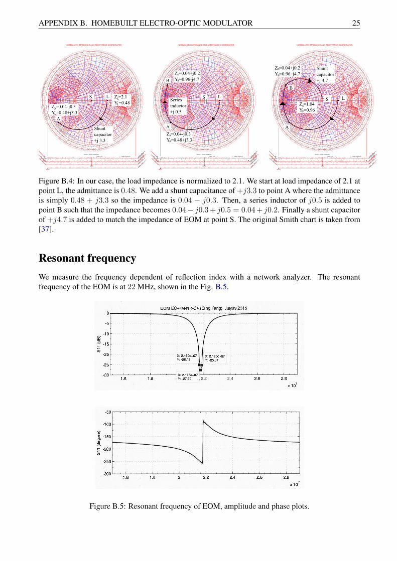
Figure B.4: In our case, the load impedance is normalized to 2.1. We start at load impedance of 2.1 atpoint L, the admittance is 0.48. We add a shunt capacitance of +j3.3 to point A where the admittanceis simply 0.48 + j3.3 so the impedance is 0.04 − j0.3. Then, a series inductor of j0.5 is added topoint B such that the impedance becomes 0.04− j0.3 + j0.5 = 0.04 + j0.2. Finally a shunt capacitorof +j4.7 is added to match the impedance of EOM at point S. The original Smith chart is taken from[37].

Resonant frequencyWe measure the frequency dependent of reflection index with a network analyzer. The resonantfrequency of the EOM is at 22 MHz, shown in the Fig. B.5.

Figure B.5: Resonant frequency of EOM, amplitude and phase plots.

Appendix C

Injection-locked diode laser

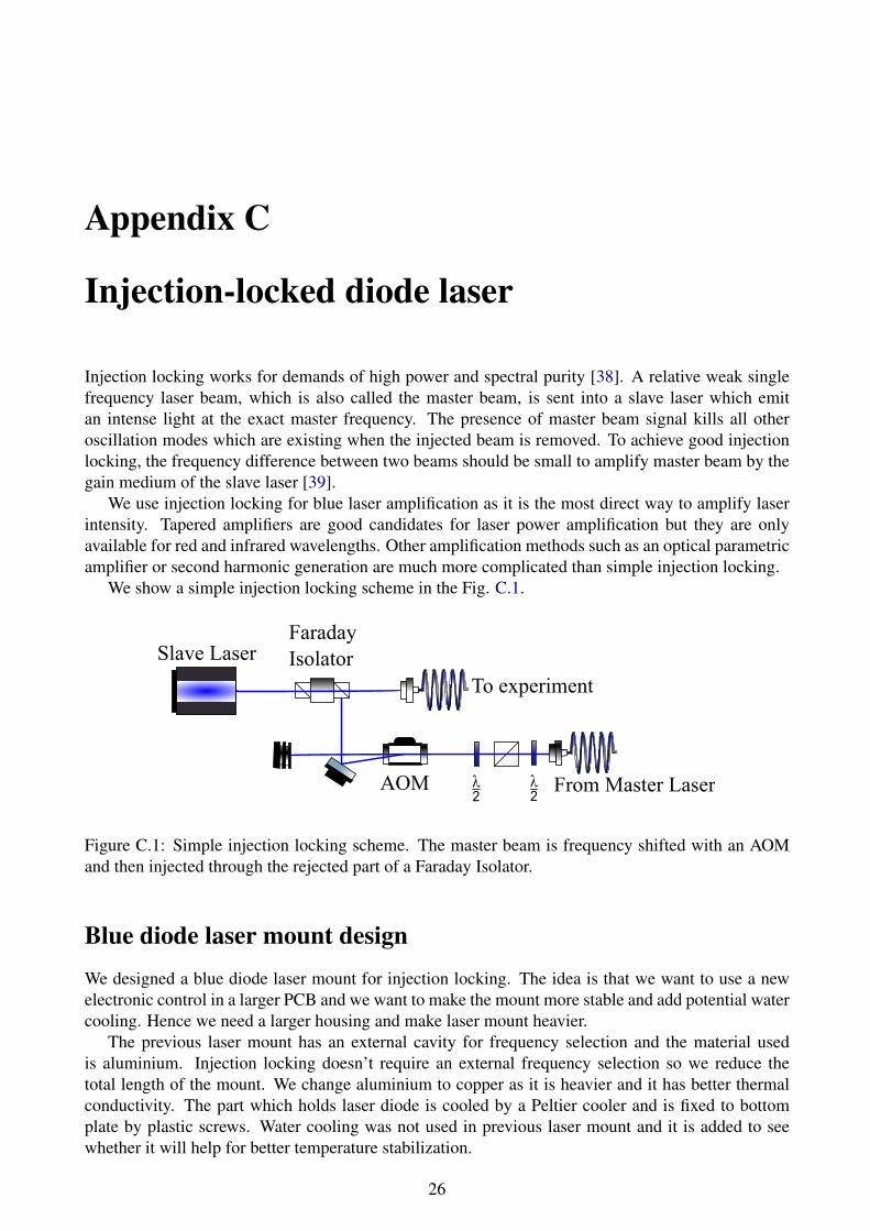
Injection locking works for demands of high power and spectral purity [38]. A relative weak singlefrequency laser beam, which is also called the master beam, is sent into a slave laser which emitan intense light at the exact master frequency. The presence of master beam signal kills all otheroscillation modes which are existing when the injected beam is removed. To achieve good injectionlocking, the frequency difference between two beams should be small to amplify master beam by thegain medium of the slave laser [39].

We use injection locking for blue laser amplification as it is the most direct way to amplify laserintensity. Tapered amplifiers are good candidates for laser power amplification but they are onlyavailable for red and infrared wavelengths. Other amplification methods such as an optical parametricamplifier or second harmonic generation are much more complicated than simple injection locking.

We show a simple injection locking scheme in the Fig. C.1.

2 2

Faraday

IsolatorSlave Laser

AOM From Master Laser

To experiment

Figure C.1: Simple injection locking scheme. The master beam is frequency shifted with an AOMand then injected through the rejected part of a Faraday Isolator.

Blue diode laser mount designWe designed a blue diode laser mount for injection locking. The idea is that we want to use a newelectronic control in a larger PCB and we want to make the mount more stable and add potential watercooling. Hence we need a larger housing and make laser mount heavier.

The previous laser mount has an external cavity for frequency selection and the material usedis aluminium. Injection locking doesn’t require an external frequency selection so we reduce thetotal length of the mount. We change aluminium to copper as it is heavier and it has better thermalconductivity. The part which holds laser diode is cooled by a Peltier cooler and is fixed to bottomplate by plastic screws. Water cooling was not used in previous laser mount and it is added to seewhether it will help for better temperature stabilization.

26

APPENDIX C. INJECTION-LOCKED DIODE LASER 27

Figure C.2: Illustration of the blue diode laser mount. Four main parts are shown as A, B, C and D inthe figure. The copper block A is used to hold the laser diode collimation package and is attached byplastic screws from the baseplate B. The baseplate is heavy and provides good mechanical stability.Additionally, the baseplate can be water-cooled using the connectors C, which might help to achievebetter temperature stability. The diode laser is encased in a plastic housing (D) to prevent temperaturefluctuation from air flows.

Acknowledgements

It is an adventure for me to join the construction of the strontium experiment. I would like to thankmy supervisor Sebastian Blatt and the team leader Immanuel Bloch for giving me this opportunity tofinish the internship for my Master’s degree. It is a fantastic environment for research and study.

I would like to thank Sebastian for his supervision, advice, trust and patience. Sebastian has aextremely profound understanding not only in physics but also how to construct a new lab. I acknowl-edge his kind guidance in my work.

Nejc Janša has shared with me his experience, knowledge besides our office. It was a pleasure towork together and he helped me a lot. I thank him for every project we have worked on.

I would like to thank Rodrigo G. Escudera, Zhichao Guo, Yunpeng Ji and Stepan Snigirev for theirkind help. All the technicians, Anton Mayer, Oliver Mödl and Karsten Förster, thank you for yourexcellent electronic and mechanic works. I would like to thank people in other labs for their supportof knowledge and every electronic and optic component. Thanks to Zhenkai Lu and Jae-yoon Choifor their kind discussion and advice.

Finally, I would like to thank my parents for their encouragement and continuous support.

28

Bibliography

[1] I. Bloch, J. Dalibard and S. Nascimbène, Quantum simulations with ultracold quantum gases,Nature Physics 8, 267 276 (2012)

[2] H. Katori, Optical lattice clocks and quantum metrology, Nature Photonics 5, 203-210 (2011)

[3] A. J. Daley, M. M. Boyd, J. Ye, and P. Zoller, Quantum Computing with Alkaline-Earth-MetalAtoms, Phys. Rev. Lett. 101, 170504 (2008)

[4] A. V. Gorshkov, A. M. Rey, A. J. Daley, M. M. Boyd, J. Ye, P. Zoller, and M. D. Lukin, Alkaline-Earth-Metal Atoms as Few-Qubit Quantum Registers, Phys. Rev. Lett. 102, 110503 (2009)

[5] L. Carr, D. DeMille, R. Krems, and J. Ye, Cold and ultracold molecules: science, technologyand applications, New J. Phys. 11, 055049 (2009)

[6] M. Greiner, M. O. Mandel, T. Esslinger, T. Hänsch, and I. Bloch, Quantum phase transitionfrom a superfluid to a Mott insulator in a gas of ultracold atoms Nature 415, 39-44 (2002)

[7] S. Kraft, F. Vogt, O. Appel, F. Riehle, and U. Sterr, Bose-Einstein Condensation of AlkalineEarth Atoms: 40Ca Phys. Rev. Lett. 103, 130401 (2009)

[8] A. H. Hansen, A. Khramov, W. H. Dowd, A. O. Jamison, V. V. Ivanov, and S. Gupta, Quantumdegenerate mixture of ytterbium and lithium atoms Phys. Rev. A 84, 011606 (2011)

[9] J. E. Sansonetti and G. Nave, Wavelengths, Transition Probabilities, and Energy Levels for theSpectrum of Neutral Strontium (Sr I), J. Phys. Chem. Ref. Data 39, 033103 (2010)

[10] A. D. Ludlow, M. M. Boyd, J. Ye, E. Peik, and P.O. Schmidt, Optical atomic clocks, Rev. Mod.Phys. 87, 637 (2015)

[11] S. Stellmer, F. Schreck, T. C. Killian, Degenerate quantum gases of strontium,arXiv:1307.0601v2 [cond-mat.quant-gas] (2014)

[12] E. S. Shuman, J. F. Barry, D. R. Glenn, and D. DeMille, Radiative Force from Optical Cyclingon a Diatomic Molecule, Phys. Rev. Lett. 103, 223001 (2009)

[13] X. Xu, T. H. Loftus, J. L. Hall, A. Gallagher, and J. Ye, Cooling and trapping of atomic stron-tium, J. Opt. Soc. Am. B 20, 968-976 (2003)

[14] M. J. Weber, Handbook of laser wavelengths, CRC Press, ISBN 978-0-849-32513-7 (1999)

[15] S. Stellmer, Degenerate quantum gases of strontium, PhD thesis, Physics department, Universityof Innsbruck (2013)

[16] T. Kurosu and F. Shimizu, Laser Cooling and Trapping of Calcium and Strontium, Jpn. J. Appl.Phys. 29 L2127 (1990)

29

30 BIBLIOGRAPHY

[17] R. Loudon, The Quantum Theory Of Light, Oxford University Press; third edition (2000), ISBN978-0-198-50176-3 (2000)

[18] M. O. Scully, Quantum Optics, Cambridge university press, ISBN 978-7-506-24966-9 (2000)

[19] H. J. Metcalf and P. Straten, Laser cooling and trapping, Springer, first edition, ISBN 978-0-387-98728-6 (1999)

[20] W. Ertmer, R. Blatt, J. Hall, and M. Zhu, Laser Manipulation of Atomic Beam Velocities:Demonstration of Stopped Atoms and Velocity Reversal, Physical Review Letters 54, 996 (1985)

[21] V. I. Balykin, V. G. Minogin, V. S. Letokhov, Electromagnetic trapping of cold atoms, Rep.Prog. Phys. 63, 1429 (2000)

[22] C. J. Foot, Atomic physics, Oxford Univ. Press, first edition, ISBN 978-0-19-850696-6 (2005)

[23] L. B. Loeb, The kinetic theory of gases, Dover Phoenix editions, ISBN 978-0-486-49572-9(2004)

[24] J. F. O’Hanlon, A User’s Guide to Vacuum Technology, Wiley-Interscience, third edition, ISBN978-0-471-27052-2 (2003)

[25] D. J. McCarron, S. A. King, S. L. Cornish, Modulation transfer spectroscopy in atomic rubid-ium, Meas. Sci. Technol. 19, 105601 (2008)

[26] D. Meschede, Optics, Light and Lasers, Wiley VCH, second, Revised and Enlarged Editionedition, ISBN 978-3-527-40628-9 (2007)

[27] W. Demtröder, Laser spectroscopy: Vol. 2: Experimental Techniques, Springer, fourth edition,ISBN 978-3-540-74952-3 (2008)

[28] G. Camy, Ch. J. Bordé, M. Ducloy, Heterodyne Saturation Spectroscopy Through FrequencyModulation Of The Saturating Beam, Opt. Comm., vol. 41, no. 5, pp. 325-330, (1978)

[29] J. H. Shirley, Modulation transfer processes in optical heterodyne saturation spectroscopy, Opt.Lett. 7, 537 (1982)

[30] A. Schenzle, R. G. DeVoe and R. G. Brewer, Phase modulation laser spectroscopy, Phys. Rev.A 25, 2606 (1982)

[31] W. Nagourney, Quantum electronics for atomic physics and telecommunication, Oxford Univer-sity Press, second edition, ISBN 978-0-199-66548-8 (2014)

[32] C. Laflamme, W. Evans, M. Dalmonte, U. Gerber, H. Mejía-Díaz, W. Bietenholz, U.-J. Wieseand P. Zoller, CP(N-1) Quantum Field Theories with Alkaline-Earth Atoms in Optical Lattices,arXiv:1507.06788 [quant-ph]

[33] U.-J. Wiese, Ultracold quantum gases and lattice systems: quantum simulation of lattice gaugetheories, Ann. Phys., 525: 777 796 (2013)

[34] Y. R. Shen, The Principles of Nonlinear Optics, Wiley-Interscience, first edition, ISBN 978-0-471-43080-3 (2002)

[35] K. K. Wong, Properties of lithium niobate, The Institution of Engineering and Technology, firstedition, ISBN 978-0-852-96799-7 (2002)

R. W. Boyd, Nonlinear optics, Academic Press, third edition, ISBN 978-0-123-69470-6 (2008)

BIBLIOGRAPHY 31

[36] C. Bowick, RF circuit design, Newnes, second edition, ISBN 978-0-750-68518-4

[37] Smith chart taken from website: http://www.dartmouth.edu/ sullivan/colorsmith.pdf

[38] G. R. Hadley, Injection locking of diode lasers, IEEE J. Quantum Electron. QE-22, 419 (1986)

[39] C. E. Wieman and L. Hollberg, Using diode lasers for atomic physics, Rev. Sci. Instrum. 62, 1(1991)