Modulation instability, Cherenkov radiation and FPU recurrence

J. M. Soto-CrespoInstituto de Optica, C.S.I.C., Serrano 121, 28006 Madrid, Spain

A. Ankiewicz, N. Devine and N. AkhmedievOptical Sciences Group, Research School of Physics and Engineering,The Australian National University, Canberra ACT 0200, Australia

We study, numerically, the influence of third-order dispersion (TOD) on modulation instability(MI) in optical fibers described by the extended nonlinear Schrodinger equation. We consider twoMI scenarios. One starts with a continuous wave (CW) with a small amount of white noise, whilethe second one starts with CW with a small harmonic perturbation at the highest value of thegrowth rate. In each case, the MI spectra show an additional spectral feature that is caused byCherenkov radiation. We give an analytic expression for its frequency. Taking a single frequencyof modulation instead of a noisy CW leads to the Fermi-Pasta-Ulam (FPU) recurrence dynamics.In this case, the radiation spectral feature multiplies due to the four-wave mixing process. FPUrecurrence dynamics is quite pronounced at small values of TOD, disappears at intermediate valuesand is restored again at high TOD when the Cherenkov frequency enters the modulation instabilityband. Our results may lead to a better understanding of the role of TOD in optical fibers.

I. INTRODUCTION

Third-order dispersion (TOD) plays an important rolein optical wave propagation in optical fibers. TOD is theorigin of the generation of Cherenkov radiation by soli-tons [1]. It serves as a seeding source for super-continuumgeneration in optical fibres pumped by continuous waves[2]. It causes the emission of optical rogue waves [3, 4]. Itis also the reason for the amplification of strong solitonsat the expense of weak ones [5]. There have been quitea few theoretical and experimental works devoted to thestudy of third-order dispersion and its influence on soli-tons [6–8]. Recently, Droques et al. [9] undertook an ex-perimental investigation of modulation instability in thepresence of TOD. They observed symmetry-breaking ofthe MI spectrum in optical fibers, and, more importantly,an additional spectral feature that appears in otherwise-typical MI spectra. This is a new phenomenon that theauthors confirmed numerically. However, the nature ofthis spectral feature still needs a solid theoretical back-ground and physical explanations. Such explanations areprovided in our present work.

Modulation instability (MI) is an interesting and richphenomenon that has attracted the attention of scientistsin various fields again and again [10–17]. This subjecthas usually been addressed in two different ways. In onecase, modulation instability develops from a noisy back-ground when the initial condition is a CW with a pertur-bation that contains all possible frequencies of modula-tion. Then the initial stage of evolution is dominated bythe component with the largest growth rate. However,all other frequencies also grow, although at a slower pace[18]. The resulting widening of spectra is the first step forsuper-continuum generation in optical fibers. The secondapproach to this challenge consists of perturbing the ini-tial CW with a single frequency of modulation. Whensolving this problem, fundamental phenomena like FPU

recurrence [19, 20] and sophisticated higher-order MI ef-fects [21, 22] have been revealed.

Clearly, the question of how TOD influences each ofthese two regimes also has to be split into two parts.In this work, we consider each case separately, in orderto build a complete picture of the influence of TOD onmodulation instability. Such a complex approach hasallowed us to reveal new and unexpected ways of howTOD influences the evolution of waves that start withthe standard MI.

II. BASIC EQUATIONS

The most common dimensional form of the nonlinearSchrodinger equation (NLSE) for waves in optical fibersclose to the zero dispersion point is [23–25]

iΨZ −β(2)

2ΨTT +

n2ω0

c|Ψ|2Ψ = i

β(3)

6ΨTTT , (1)

where Ψ is the amplitude of the slowly-varying envelopeof the optical field, β(n) is the n-th order dispersion pa-rameter [i.e., β(n) = ∂nβ/∂ωn evaluated at the carrierfrequency ω0], n2 is the nonlinear index of refractionwhile c is the speed of light.

By using the transformation:

z = Z/λ, t = T/√λ, ψ =

√n2/(2π)Ψ, (2)

where λ is the wavelength, Eq.(1) can be reduced to itsnormalized form

iψz +β2

2ψtt + |ψ|2ψ = iβ3ψttt, (3)

where

β2 = −β(2), β3 =β(3)

6√λ

(4)

2

When β3 is zero, equation (3) becomes the standardNLSE, which is integrable. Reversing the transforma-tions (2) we can always return to dimensional units.

The continuous wave (CW) solution of Eq.(3) is

ψ = AeiA2z (5)

Without loss of generality, we can take A = 1, as we canalways use the scaling transformation [8] to return to anarbitrary amplitude.

In the absence of TOD, and for positive β2, equation(3) has a family of solutions that are presently known asAkhmediev breathers (AB) [26, 27]. By choosing β2 = 1without losing any generality, they are given by

ψ(t, z) =

[1−

Ω2

2 cosh(δz) + iδ sinh(δz)

cosh(δz)− δΩ cos(Ωt)

]exp(iz). (6)

This equation defines a family of solutions. The free pa-rameter of the family is Ω; it varies in an interval between0 to 2 and defines the frequency of the initial modulationΩ and the initial growth rate of the modulation:

δ = Ω

√1− Ω2

4.

When z → ±∞, this solution becomes the plane waveeiz+iφ with different phases φ at the two limits. Takinginto account the lowest-order modulated terms, Eq.(6)can be approximated at z → −∞ by

ψ(t, z) =

[1− µδ

(Ω + i

2δ

Ω

)eδz cos(Ωt)

]eiz+iφ, (7)

where µ is a small real parameter and φ is the initialphase of the CW. The exponential factor eδz in (7) clearlyshows that the solution (6) starts from modulation in-stability. Using (7) as the initial condition in simulatingwave propagation, we can recover the solution (6). Ignor-ing the complex factor when taking a small amplitude µshifts the simulations from the exact heteroclinic orbit toa nearby periodic solution. We note that there is a non-linear phase shift related to recurrence [28] which makesthe trajectory heteroclinic rather than homoclinic.

The discrete spectral components of (6) evolve accord-ing to [6, 18]:

A0(z) = 1− iδ sinh(δz) + (Ω2/2) cosh(δz)√cosh2(δz)− δ2

Ω2

(8)

An(z) =iδ sinh δz + (Ω2/2) cosh(δz)√

cosh2(δz)− δ2

Ω2

(9)

×

Ωcosh(δz)−

√cosh2(δz)− δ2

Ω2

δ

|n|

where Ω and δ are the same as above. On a logarithmicscale, the spectrum has a triangular shape [18], thoughwe must remember that it is discrete.

An interesting question has been raised in the recentwork of Mahnke and Mitschke [26]. Namely, how sta-ble are ABs relative to various perturbations? The au-thors have found that perturbations of the wave field gov-erned by the NLSE do not destroy ABs. On the otherhand, perturbing the NLSE with a small Raman termsplits ABs into solitons - a process which is an essentialpart of super-continuum generation in fibers. Generallyspeaking, other perturbations that lift integrability of theNLSE should lead to similar dynamics. TOD would beone of these perturbations. However, the influence ofTOD is more complicated, as we can see from our sim-ulations presented below. In order to see these compli-cations, we have to look deeper into the mechanism ofradiation.

III. RESONANT RADIATION AND ITSFREQUENCY

It is well-known that TOD creates radiation waves[1]. Generally, only t-dependent solutions produce radia-tion. A CW solution by itself does not produce radiationwaves. They appear only when the CW is split into sep-arate pulses according to (6). As a result, we can viewsmall amplitude radiation waves as being generated justas occurs in the soliton case. Here, we use the NLSE inthe form given by Eq.(3). Then, we can represent disper-sive waves in the form

ψ = µei(kz−ωt), (10)

where µ is a small amplitude and k is the propagationconstant. The frequency then satisfies the dispersion re-lation

−k − ω2β2/2 = −β3ω3 (11)

In order for this radiation to be resonant with the ABsolution which serves as the source of the radiation, itspropagation constant should coincide with that of theAB. This is a condition for Cherenkov radiation and it isgiven by k = A2 = 1.

Thus, the condition for the resonance is

A2 = 1 = −ω2β2/2 + β3ω3, (12)

and we have the following cubic equation to solve:

ω3 − β2

2β3ω2 − 1

β3= 0. (13)

Eq.(13) can be solved analytically [29]. For positive β2,among the three roots, two are complex conjugates andone is purely real. The sign of the real root coincideswith the sign of β3. This real solution

ω =χ2 + β2χ+ β2

2

6β3χ(14)

3

where χ =(β3

2 + 108β23 + 6

√6√β3

2β23 + 54β4

3

)1/3

pro-

vides us with the resonant condition for dispersive linearwaves created by an AB. Despite being only an approx-imation, our simulations presented below show that theresonant frequency is accurately fitted by this equation.

The numerical simulations are done by solving Eq.(3)with initial conditions consisting of a constant amplitudefield plus small complex amplitude white noise. To beprecise:

ψ(z = 0, t) = 1 + a(t) + ib(t), (15)

where a(t) and b(t) are two uncorrelated real randomfunctions which take values uniformly distributed in asmall interval around 0. This initial condition leads tomodulation instability within the instability band so thatthe sidebands inside the gain bandwidth, i.e. for |ω| < 2,increase their amplitudes exponentially during the initialstages of propagation according to (7). We have chosenthe propagation distance to be z = 20, which correspondsto a short fiber, so that the spectral component that hasthe highest growth rate dominates the evolution. Logi-cally, for each realization, when using specific values ofthe random functions a and b, and for fixed propagationdistance, the spectrum appears to be noisy. In order tohave uniform results, we have averaged the output spec-tra for a minimum of 100 different realizations. Then theaverage output spectra are smooth, and the simulationscan mimic actual experiments undertaken in ([9]).

−15 0 15

01

2β

2

0

5

10

15

β 3 = 0 . 0 1

ω

Sp

ec

tra

l in

ten

sity

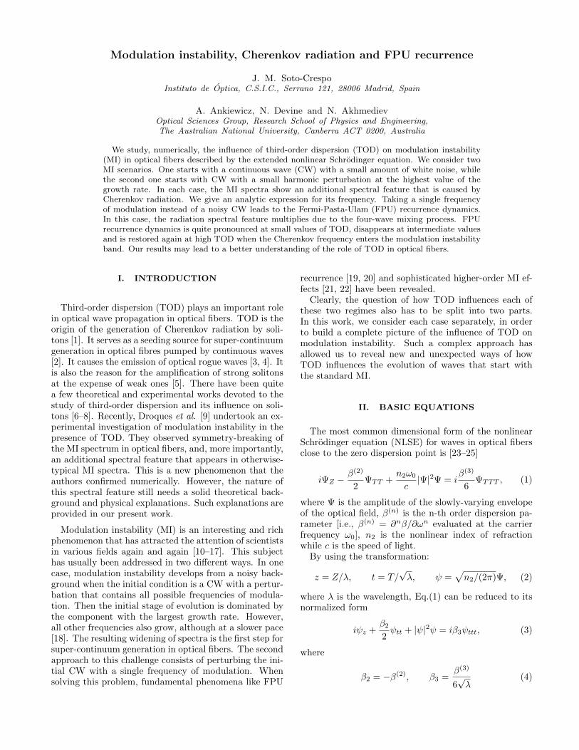
FIG. 1. (Color online) Spectral output intensity for a propa-gation distance z = 20, β3 = 0.01 and for various values of β2.The two sidebands are related to modulation instability, whilethe additional spectral band on the right represents the reso-nant radiation. The green dashed line, defined by Eq.(14), isin perfect agreement with the numerical simulations.

Here, we are interested in the average spectral out-put of the optical fiber versus the dispersion coefficients.Such data would describe the type of experiment pre-sented in [9]. Figure 1 shows the shapes of the spectraat an early fixed stage of MI evolution for various valuesof β2. The value of β3 = 0.01 here is taken to be smalland fixed. The total propagation distance is also fixed atz = 20. The spectral component, additional to the stan-dard MI sidebands, that appears on the right-hand-sideof the spectra in Fig.1 is caused by TOD, and is well-approximated by Eq.(14). The latter is shown by thegreen dashed curve. As we can see from this figure, thelocation of the resonant frequency is perfectly describedby this simple result. Our theory is also in agreementwith the numerical and the experimental results of thework [9]. Note that the axis of β2 of Figures 1 and 2 of[9] is inverted - the value of β2 grows downwards, whichis opposite to our choice.

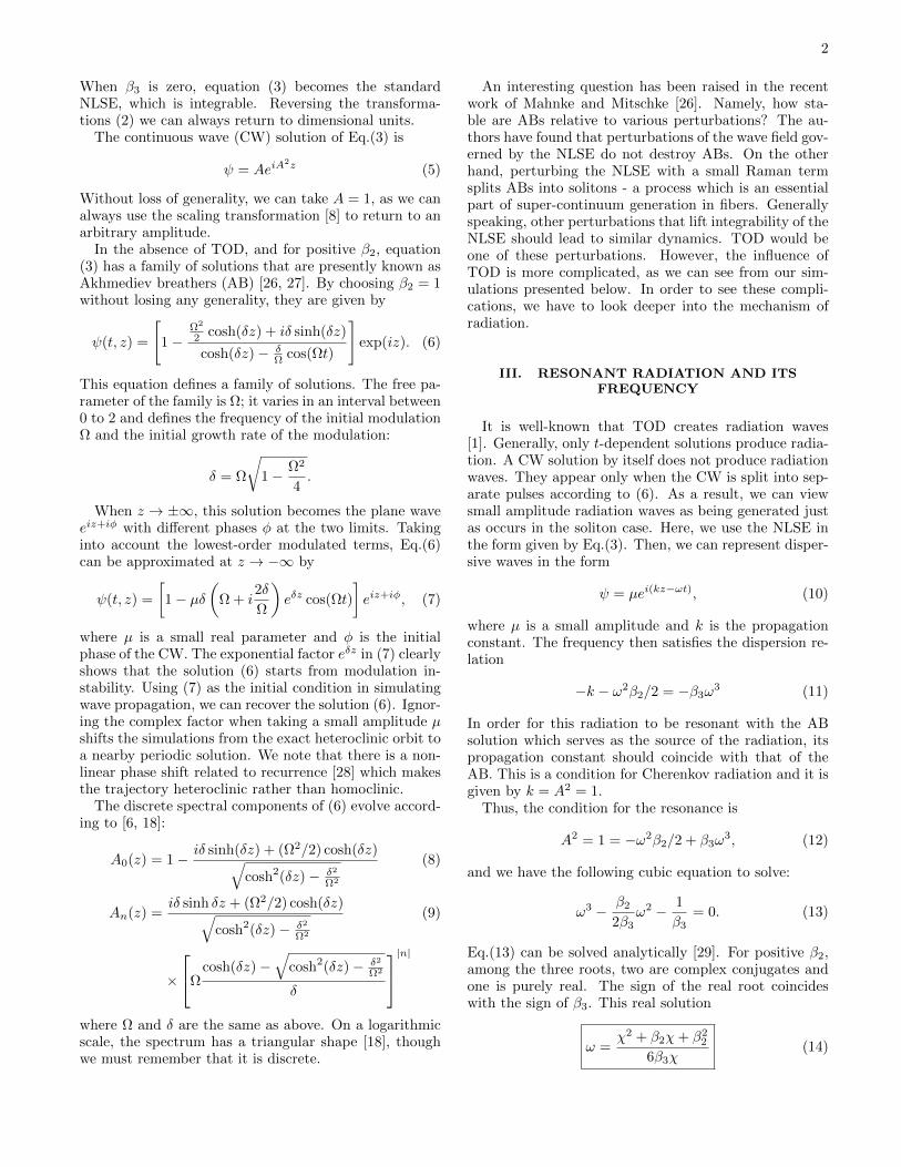
Another set of data is presented in Figure 2. Here, wehave kept the value of β2 = 1 constant while β3 is changedfrom 0 to 1. The resonant frequency of dispersive wavesis seen on the right-hand-side of the spectrum. It ap-proaches the MI sideband monotonically while β3 growsfrom 0 to 1. The calculation giving the white dashedcurve is based on Eq.(14). It approximates reasonablywell the spectral feature caused by the dispersive wavesat small values of β3 when the MI evolves according tothe unperturbed NLSE. Higher values of β3 significantlyinfluence the basic process of MI.

FIG. 2. (Color online) Spectral intensity output of the fiberfor a propagation distance of z = 20 and β2 = 1, as a functionof β3. The white dashed line is given by Eq.(14).

4

IV. INFLUENCE OF RADIATION ON FPURECURRENCE

The influence of dispersive waves on the MI spectra isclearly seen at small propagation distances. What willhappen when the distances increase? FPU recurrencewas observed experimentally by Van Simaeys et al. in[19]. Will it also be seen here? Preliminary studies inthis regard have been carried out in [6]. Here, we give amore detailed answer to the above question.

It is well-known that modulation instability in theNLSE, when started with a single sideband, results inrecurrence. This is called Fermi-Pasta-Ulam recurrence:the dynamical system returns to the same state of sin-gle mode excitation from which the dynamics started.This process is perfectly described by the AB solution(6) [20, 28]. Observation of the FPU recurrence requiresmore accurate initial conditions than in (15). We haveto use strictly periodic initial conditions like (7), ratherthan CW with a random perturbation. Thus, as initialconditions in the numerical simulations below, we took aconstant amplitude field, slightly modulated with a fre-quency ω located within the instability band:

ψ(z = 0, t) = 1 + µ cos(ωt), (16)

where µ is a small constant. With this initial conditionand µ complex, as in (7), and with β3 = 0, the fieldgoverned by the NLSE evolves according to Eq.(6). De-viations from the exact initial conditions, such as takingµ to be real instead of complex, results in a deviationfrom the exact heteroclinic trajectory, thus producingperiodic evolution. In the following simulations we usesmall µ = 0.0001, and ω =

√2. This frequency produces

the highest MI gain for a field amplitude 1. Here, and inthe rest of the paper, we assume β2 = 1.

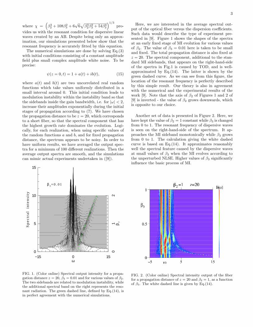
Now, we turn to the case of nonzero β3. Figure 3 showsthe spectrum evolution of the solution that starts withthe initial condition (16). For a small value of β3 (=0.01),the solution is close to (6) with a spectrum close to thatdefined in (8). The first expansion of the spectrum atz ≈ 10 is indeed very close to the analytic expression.The spectrum starts to evolve periodically as the hete-roclinic orbit is transformed to periodic motion for anysmall perturbation. A small amplitude spectral feature,corresponding to the dispersive waves, is clearly seen onthe right-hand-side of the spectrum. The value of theradiation frequency is indeed given by the resonant con-dition (14). It is indicated by the blue dashed verticalline in this figure. The radiation component grows dur-ing propagation, as some is emitted each time when theoptical field splits into pulses. For the small value ofβ3 considered in this example, the influence of radiationon the AB is almost negligible. Thus, recurrence to theplane wave occurs for many periods of evolution. Threeof them can be seen in Figure 3, and periodic evolutioncontinues well after z = 50.

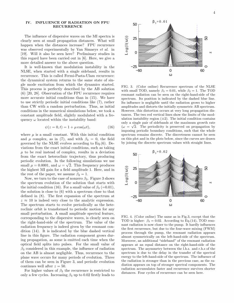
For higher values of β3 the recurrence is restricted toonly a few cycles. Increasing β3 up to 0.02 firstly leads to

−60 0 60

050

z

−25

0

25

50β 3 = 0 . 0 1

ω

Lo

g(I

(ω))

FIG. 3. (Color online) Recurrence spectrum of the NLSEwith small TOD, namely β3 = 0.01, while β2 = 1. The TODresonant radiation can be seen on the right-hand-side of thespectrum. Its position is indicated by the dashed blue line.Its influence is negligible until the radiation grows to higheramplitudes and distorts the initially symmetric AB spectrum.However, this distortion occurs at very long propagation dis-tances. The two red vertical lines show the limits of the mod-ulation instability region (±2). The initial condition containsonly a single pair of sidebands at the maximum growth rate(ω =

√2. The periodicity is preserved on propagation by

imposing periodic boundary conditions, such that the wholespectrum remains discrete. The discreteness cannot be seenon this plot and in the plots below, since the curves are drawnby joining the discrete spectrum values with straight lines.

−60 0 600

50z

−25

0

25

50β 3 = 0 . 0 2

ω

Lo

g(I

(ω))

FIG. 4. (Color online) The same as in Fig.3, except that theTOD is higher: β3 = 0.02. According to Eq.(14), TOD reso-nant radiation is now closer to the pump. It hardly influencesthe first recurrence, but due to the four-wave mixing (FWM)process through the pump, the resonant radiation appearsalmost symmetrically on the left-hand-side of the spectrum.Moreover, an additional “sideband” of the resonant radiationappears at an equal distance on the right-hand-side of thespectrum. The asymmetry between the l.h.s. and r.h.s of thespectrum is due to the delay in the transfer of the spectralenergy to the left-hand-side of the spectrum. The influence ofthe radiation is stronger than in the previous case, as the ra-diation appears on top of stronger spectral components. Theradiation accumulates faster and recurrence survives shorterdistances. Four cycles of recurrence can be seen here.

5

the shift of the resonant frequency, which becomes closerto the pump frequency. Secondly, it leads to the intensityincrease of the radiation waves. The results are shownin Fig.4. Another significant difference from the previ-ous case is that the resonant radiation also appears onthe left-hand-side of the spectrum due to the four-wave-mixing (FWM) process. These radiation components ofthe spectrum are repeated at equal spectral intervals onthe left and right-hand-sides of the initial resonant fre-quency. The latter is indicated by the vertical dashedblue line. As a result, we obtain an equi-distantly lo-cated comb of dispersive spectral components on top ofthe original AB spectrum, with amplitudes that growcontinuously, but very slowly. These components arehardly visible at the first appearance of the triangularAB spectrum, but they significantly disturb the triangu-lar spectra repeatedly appearing in the subsequent evolu-tion. The level of disturbance is still small for β3 = 0.02,and clear FPU recurrence can be observed at least fourtimes in this figure. The period in z is reduced here dueto a higher level of deviation from the heteroclinic tra-jectory.

−60 0 60

050

z

−25

0

25

50β 3 = 0 . 0 4

ω

Lo

g(I

(ω))

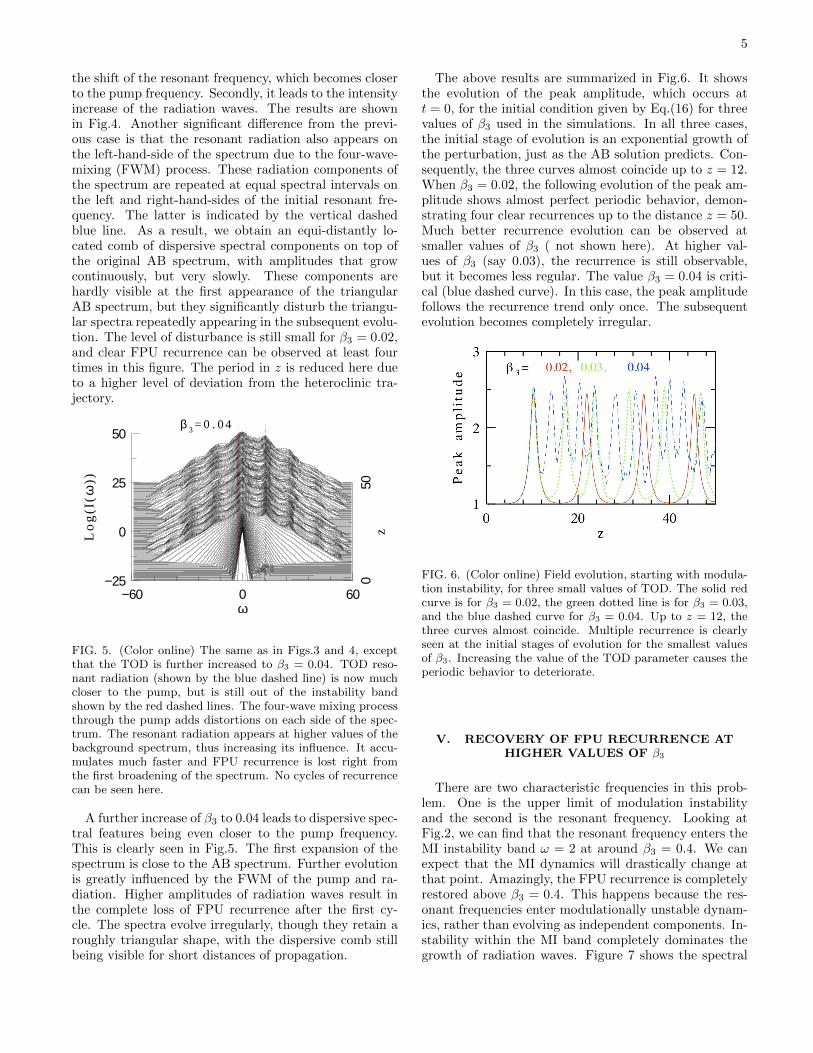
FIG. 5. (Color online) The same as in Figs.3 and 4, exceptthat the TOD is further increased to β3 = 0.04. TOD reso-nant radiation (shown by the blue dashed line) is now muchcloser to the pump, but is still out of the instability bandshown by the red dashed lines. The four-wave mixing processthrough the pump adds distortions on each side of the spec-trum. The resonant radiation appears at higher values of thebackground spectrum, thus increasing its influence. It accu-mulates much faster and FPU recurrence is lost right fromthe first broadening of the spectrum. No cycles of recurrencecan be seen here.

A further increase of β3 to 0.04 leads to dispersive spec-tral features being even closer to the pump frequency.This is clearly seen in Fig.5. The first expansion of thespectrum is close to the AB spectrum. Further evolutionis greatly influenced by the FWM of the pump and ra-diation. Higher amplitudes of radiation waves result inthe complete loss of FPU recurrence after the first cy-cle. The spectra evolve irregularly, though they retain aroughly triangular shape, with the dispersive comb stillbeing visible for short distances of propagation.

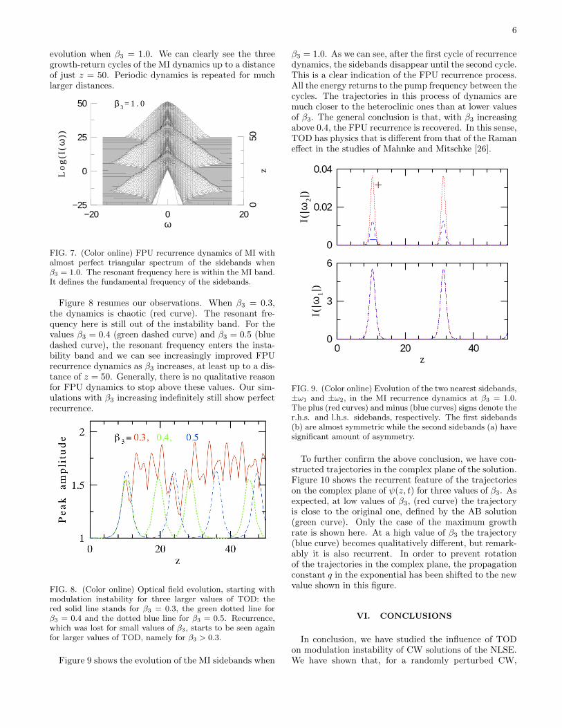
The above results are summarized in Fig.6. It showsthe evolution of the peak amplitude, which occurs att = 0, for the initial condition given by Eq.(16) for threevalues of β3 used in the simulations. In all three cases,the initial stage of evolution is an exponential growth ofthe perturbation, just as the AB solution predicts. Con-sequently, the three curves almost coincide up to z = 12.When β3 = 0.02, the following evolution of the peak am-plitude shows almost perfect periodic behavior, demon-strating four clear recurrences up to the distance z = 50.Much better recurrence evolution can be observed atsmaller values of β3 ( not shown here). At higher val-ues of β3 (say 0.03), the recurrence is still observable,but it becomes less regular. The value β3 = 0.04 is criti-cal (blue dashed curve). In this case, the peak amplitudefollows the recurrence trend only once. The subsequentevolution becomes completely irregular.

FIG. 6. (Color online) Field evolution, starting with modula-tion instability, for three small values of TOD. The solid redcurve is for β3 = 0.02, the green dotted line is for β3 = 0.03,and the blue dashed curve for β3 = 0.04. Up to z = 12, thethree curves almost coincide. Multiple recurrence is clearlyseen at the initial stages of evolution for the smallest valuesof β3. Increasing the value of the TOD parameter causes theperiodic behavior to deteriorate.

V. RECOVERY OF FPU RECURRENCE ATHIGHER VALUES OF β3

There are two characteristic frequencies in this prob-lem. One is the upper limit of modulation instabilityand the second is the resonant frequency. Looking atFig.2, we can find that the resonant frequency enters theMI instability band ω = 2 at around β3 = 0.4. We canexpect that the MI dynamics will drastically change atthat point. Amazingly, the FPU recurrence is completelyrestored above β3 = 0.4. This happens because the res-onant frequencies enter modulationally unstable dynam-ics, rather than evolving as independent components. In-stability within the MI band completely dominates thegrowth of radiation waves. Figure 7 shows the spectral

6

evolution when β3 = 1.0. We can clearly see the threegrowth-return cycles of the MI dynamics up to a distanceof just z = 50. Periodic dynamics is repeated for muchlarger distances.

−20 0 20

050

z

−25

0

25

50 β 3 = 1 . 0

ω

Lo

g(I

(ω))

FIG. 7. (Color online) FPU recurrence dynamics of MI withalmost perfect triangular spectrum of the sidebands whenβ3 = 1.0. The resonant frequency here is within the MI band.It defines the fundamental frequency of the sidebands.

Figure 8 resumes our observations. When β3 = 0.3,the dynamics is chaotic (red curve). The resonant fre-quency here is still out of the instability band. For thevalues β3 = 0.4 (green dashed curve) and β3 = 0.5 (bluedashed curve), the resonant frequency enters the insta-bility band and we can see increasingly improved FPUrecurrence dynamics as β3 increases, at least up to a dis-tance of z = 50. Generally, there is no qualitative reasonfor FPU dynamics to stop above these values. Our sim-ulations with β3 increasing indefinitely still show perfectrecurrence.

FIG. 8. (Color online) Optical field evolution, starting withmodulation instability for three larger values of TOD: thered solid line stands for β3 = 0.3, the green dotted line forβ3 = 0.4 and the dotted blue line for β3 = 0.5. Recurrence,which was lost for small values of β3, starts to be seen againfor larger values of TOD, namely for β3 > 0.3.

Figure 9 shows the evolution of the MI sidebands when

β3 = 1.0. As we can see, after the first cycle of recurrencedynamics, the sidebands disappear until the second cycle.This is a clear indication of the FPU recurrence process.All the energy returns to the pump frequency between thecycles. The trajectories in this process of dynamics aremuch closer to the heteroclinic ones than at lower valuesof β3. The general conclusion is that, with β3 increasingabove 0.4, the FPU recurrence is recovered. In this sense,TOD has physics that is different from that of the Ramaneffect in the studies of Mahnke and Mitschke [26].

0 20 400

3

6

z

I(|ω

1|)

0

0.02

0.04

+

_

I(|ω

2|)

FIG. 9. (Color online) Evolution of the two nearest sidebands,±ω1 and ±ω2, in the MI recurrence dynamics at β3 = 1.0.The plus (red curves) and minus (blue curves) signs denote ther.h.s. and l.h.s. sidebands, respectively. The first sidebands(b) are almost symmetric while the second sidebands (a) havesignificant amount of asymmetry.

To further confirm the above conclusion, we have con-structed trajectories in the complex plane of the solution.Figure 10 shows the recurrent feature of the trajectorieson the complex plane of ψ(z, t) for three values of β3. Asexpected, at low values of β3, (red curve) the trajectoryis close to the original one, defined by the AB solution(green curve). Only the case of the maximum growthrate is shown here. At a high value of β3 the trajectory(blue curve) becomes qualitatively different, but remark-ably it is also recurrent. In order to prevent rotationof the trajectories in the complex plane, the propagationconstant q in the exponential has been shifted to the newvalue shown in this figure.

VI. CONCLUSIONS

In conclusion, we have studied the influence of TODon modulation instability of CW solutions of the NLSE.We have shown that, for a randomly perturbed CW,

7

−2.5 0 2.5−2.5

0

2.5

β 3= 0 (q=1)

β 3= 0.02(q=1.003)

β 3=1 (q=1.088)

R e( ψ m a x( z , T ) )

Im(ψ

ma

x(z

,T))

FIG. 10. (Color online) Recurrent trajectories of MI dynamicsfor β3 = 0 (green curve), β3 = 0.02 (red curve) and β3 = 1(blue curve).

TOD results in resonant radiation waves caused by theCherenkov effect, and we have obtained a very good es-timate of the frequency of this radiation. On the otherhand, when the CW is perturbed with a single frequency,the radiation is multiplied due to the four-wave mixingeffect. This causes the normally-recurrent solution to be

converted into an aperiodic one. An interesting findingis that the periodicity is improved and the radiation dis-appears at higher values of the TOD coefficient, whenthe resonant frequency enters the modulation instabilityband.

The first part of our results have been observed in theexperimental work of Droques et al. [9], and here wehave given the theoretical background for these fascinat-ing observations, as well as supplying the frequency of theadditional peak in the spectra. Clearly, these estimatescan be used for extracting the parameters of the fiberfrom experimental data. The second part of our resultsawaits future exciting experimental observations. Theseobservations can be made at frequencies close to the zerodispersion point of the fiber, where TOD is comparableto second-order dispersion.

ACKNOWLEDGMENTS

The work of J.M.S.C. is supported by the MINECOunder contract FIS2009-09895. The authors acknowledgethe support of the Australian Research Council (Discov-ery Project number DP110102068). N.A. is a recipientof the Alexander von Humboldt Award.

[1] N. Akhmediev and M. Karlsson, Cherenkov radiationemitted by solitons in optical fibres, Phys. Rev., 51, 2602(1995).

[2] J. M. Dudley, G. Genty, F. Dias, B. Kibler, N. Akhme-diev, Modulation instability, Akhmediev Breathers andcontinuous wave supercontinuum generation, Opt. Ex-press, 17, 21497 (2009).

[3] M. Taki, A. Mussot, A. Kudlinski, E. Louvergneaux, M.Kolobov, M. Douay, Third-order dispersion for generat-ing optical rogue solitons, Physics Letters A 374 691695(2010).

[4] G. Genty, C. M. de Sterke, O. Bang, F. Dias, N. Akhme-diev, J. M. Dudley, Collisions and turbulence in opticalrogue wave formation, Physics Letters A 374, 989996(2010).

[5] N. Akhmediev, J.M. Soto-Crespo, and A. Ankiewicz,Could rogue waves be used as efficient weapons againstenemy ships?, Eur. Phys. J. Special Topics 185, 259266(2010).

[6] N. N. Akhmediev, V. I. Korneev, and N. V. Mitskevich,Modulation instability of a continuous signal in an opticalfibre taking into account third order dispersion, IzvestiyaVysshikh Uchebnykh Zavedenii, Radiofizika, Vol. 33, pp.111-117, (1990).

[7] M. I. Kolobov, A. Mussot, A. Kudlinski, E. Lou-vergneaux, and M. Taki, Third-order dispersion drasti-cally changes parametric gain in optical fiber systems,Phys. Rev. A 83, 035801 (2011).

[8] N. Akhmediev and A. Ankiewicz, ”Solitons: nonlinearpulses and beams”, Chapman & Hall, London, 1997.

[9] M. Droques, B. Barviau, A. Kudlinski, M. Taki, A.Boucon, T. Sylvestre, and A. Mussot, Symmetry-breaking dynamics of the modulational instability spec-trum, Opt. Lett., 36, 1359 (2011).

[10] V. I. Bespalov and V. I. Talanov, Filamentary structureof light beams in nonlinear liquids, JETP Lett. 3, 307-310, (1966)

[11] T. B. Benjamin and J. E. Feir, The disintegration ofwavetrains on deep water. Part 1: Theory, J. Fluid Mech.27, 417-430 (1967).

[12] G. P. Agrawal, Modulation Instability Induced by Cross-Phase Modulation, Phys. Rev. Lett., 59, 880 (1987).

[13] D. Kip, Marin Soljacic, M. Segev, E. Eugenieva, D. N.Christodoulides, Modulation Instability and Pattern For-mation in Spatially Incoherent Light Beams, Science,290, 495 (2000).

[14] A.V. Gorbach, X. Zhao, and D.V. Skryabin, Disper-sion of nonlinearity and modulation instability in sub-wavelength semiconductor waveguides, Optics Express,19, 9345 (2011).

[15] K. Porsezian, K. Senthilnathan and S. Devipriya, Mod-ulation instability in Fiber Bragg grating with non-Kerrnonlinearity, IEEE J. Quant. Electron., 41, 789 (2005).

[16] N. C. Panoiu, X. F. Chen, and R. M. Osgood, Modulationinstability in silicon photonic nanowires, Opt. Lett. 31,3609 - 3611 (2006).

[17] K. Kasamatsu and M. Tsubota, Modulation instabil-ity and solitary-wave formation in two-component Bose-Einstein condensates, Phys. Rev. A 74, 013617 (2006).

8

[18] N. Akhmediev, A. Ankiewicz, J. M. Soto-Crespoand J. M. Dudley, Universal triangular spectra inparametrically-driven systems, Phys. Lett., 375, 775(2011).

[19] G. Van Simaeys, Ph. Emplit and M. Haelterman, Exper-imental demonstration of the Fermi-Pasta-Ulam recur-rence in a modulationally unstable optical wave, Phys.Rev. Lett. 87, 033902 (2001).

[20] N. Akhmediev, Deja vu in optics, Nature, 413, No 6853,pp. 267 - 268 (2001).

[21] S. Wabnitz and N. Akhmediev, Efficient modulation fre-quency doubling by induced modulation instability, Opt.Commun. 283, 1152 (2010).

[22] M. Erkintalo, K. Hammani, B. Kibler, C. Finot, N.Akhmediev, J. M. Dudley, and G. Genty, Higher-OrderModulation Instability in Nonlinear Fiber Optics, Phys.Rev. Lett., 107, 253901 (2011).

[23] M. J. Potasek, Modulation instability in an extendednonlinear Schrodinger equation, Opt. Lett., 12, 921(1987).

[24] K. Tai, A. Hasegawa, and A. Tomita, Observation ofModnlational Instability in Optical Fibers, Phys. Rev.Lett., 56, 135 (1986).

[25] Solange B. Cavalcanti, Jose C. Cressoni, Heber R. daCruz, and Artur S. Gouveia-Neto, Modulation instabil-ity in the region of minimum group-velocity dispersionof single-mode optical fibers via an extended nonlinearSchrodinger equation, Phys. Rev. A 43, 6162 (1991).

[26] Ch. Mahnke and F. Mitschke, Possibility of an Akhme-diev breather decaying into solitons, Phys. Rev. A 85,033808 (2012).

[27] M. Erkintalo, G. Genty, B. Wetzel, J. M. Dudley, Akhme-diev breather evolution in optical fiber for realistic initialconditions, Phys. Lett., A 375, 2029 (2011).

[28] N. Devine, A. Ankiewicz, G. Genty, J.M. Dudley, N.Akhmediev, Recurrence phase shift in FermiPastaUlamnonlinear dynamics, Phys. Lett. A, 375, 4158 - 4161(2011).

[29] M. Abramowitz and I. A. Stegun, Handbook of mathe-matical functions with formulas, graphs and mathemati-cal tables, (Dover publications, NY, 1972).