modularization and validation of fun3d as a create · pdf fileamerican institute of...

American Institute of Aeronautics and Astronautics

1

Modularization and Validation of FUN3D as a CREATE-AV Helios Near-body Solver

Rohit Jain1 US Army Aviation Development Directorate - AFDD

Aviation & Missile Research, Development & Engineering Center Research, Development and Engineering Command (RDECOM)

Moffett Field, California

Robert T. Biedron2 William T. Jones3

Elizabeth M. Lee-Rausch4 Computational AeroSciences Branch – MS 128

NASA Langley Research Center, Hampton, Virginia

Under a recent collaborative effort between the US Army Aeroflightdynamics Directorate (AFDD) and NASA Langley, NASA's general unstructured CFD solver, FUN3D, was modularized as a CREATE-AV Helios near-body unstructured grid solver. The strategies adopted in Helios/FUN3D integration effort are described. A validation study of the new capability is performed for rotorcraft cases spanning hover prediction, airloads prediction, coupling with computational structural dynamics, counter-rotating dual-rotor configurations, and free-flight trim. The integration of FUN3D, along with the previously integrated NASA OVERFLOW solver, lays the ground for future interaction opportunities where capabilities of one component could be leveraged with those of others in a relatively seamless fashion within CREATE-AV Helios.

Nomenclature 𝑎𝑎∞ = freestream speed of sound, 𝑓𝑓𝑓𝑓/𝑠𝑠 𝑐𝑐 = blade local chord, 𝑖𝑖𝑖𝑖 𝑐𝑐𝑡𝑡𝑡𝑡𝑡𝑡 = blade tip chord, 𝑖𝑖𝑖𝑖 𝐶𝐶𝑃𝑃 = rotor power coefficient, 𝐶𝐶𝑃𝑃 ≡ 𝐶𝐶𝑄𝑄 𝐶𝐶𝑄𝑄 = rotor torque coefficient, 𝑄𝑄

𝜋𝜋𝜋𝜋Ω2𝑅𝑅5

𝐶𝐶𝑇𝑇 = rotor thrust coefficient, 𝑇𝑇𝜋𝜋𝜋𝜋Ω2𝑅𝑅4

1 Aerospace Engineer, Senior Member AIAA 2 Senior Research Scientist, Senior Member AIAA 3 Computer Engineer, Associate Fellow AIAA 4 Research Engineer, Associate Fellow AIAA This material is declared a work of the U.S. Government and is not subject to copyright protection in the United States. DISTRIBUTION STATEMENT A. Approved for public release; distribution is unlimited.

https://ntrs.nasa.gov/search.jsp?R=20160007705 2018-05-25T05:59:18+00:00Z


2

𝐹𝐹𝐹𝐹 = figure of merit, 𝐶𝐶𝑇𝑇2𝐶𝐶𝑇𝑇𝐶𝐶𝑄𝑄

𝐹𝐹𝑁𝑁 = blade section normal force, 𝑙𝑙𝑙𝑙𝑓𝑓/𝑓𝑓𝑓𝑓 𝐹𝐹 = local Mach number 𝐹𝐹𝑡𝑡𝑡𝑡𝑡𝑡 = tip Mach number, Ω𝑅𝑅/𝑎𝑎∞ 𝐹𝐹2𝐶𝐶𝑁𝑁 = blade section normal force, 𝐹𝐹𝑁𝑁

12𝛾𝛾𝛾𝛾𝑡𝑡∞

𝑝𝑝∞ = freestream pressure, 𝑙𝑙𝑙𝑙𝑓𝑓/𝑓𝑓𝑓𝑓2 𝑟𝑟𝛾𝛾 = vortex core radius, normalized by 𝑐𝑐𝑡𝑡𝑡𝑡𝑡𝑡 𝑟𝑟 = rotor radial axis, normalized by 𝑅𝑅 𝑅𝑅 = blade radius, 𝑓𝑓𝑓𝑓 𝑅𝑅𝑒𝑒𝛾𝛾 = Reynolds number based on 𝑐𝑐𝑡𝑡𝑡𝑡𝑡𝑡 𝑄𝑄 = rotor torque, 𝑓𝑓𝑓𝑓-𝑙𝑙𝑙𝑙𝑓𝑓 𝑇𝑇 = rotor thrust, 𝑙𝑙𝑙𝑙𝑓𝑓 𝑉𝑉∞ = freestream speed, 𝑓𝑓𝑓𝑓/𝑠𝑠 𝑧𝑧 = rotor axis, normalized by 𝑅𝑅 𝛼𝛼𝑠𝑠 = rotor shaft tilt, 𝑑𝑑𝑒𝑒𝑑𝑑., positive aft 𝛾𝛾 = ratio of specific heats, = 1.4 for standard air 𝜃𝜃𝛾𝛾 = collective pitch, deg. 𝜇𝜇 = advance ratio, 𝑉𝑉∞/(Ω𝑅𝑅) 𝜌𝜌 = density, slugs/𝑓𝑓𝑓𝑓3 𝜎𝜎 = rotor solidity 𝜓𝜓 = rotor azimuth, deg., 0 at the aft

𝜔𝜔 = vorticity magnitude, normalized by Ω Ω = rotor rotational speed, 𝑟𝑟𝑎𝑎𝑑𝑑/𝑠𝑠

Introduction

elicopter Overset Simulations (Helios) [1] is a high-fidelity computational modeling framework for rotorcraft modeling. It has been developed under the sponsorship from the Department of Defense

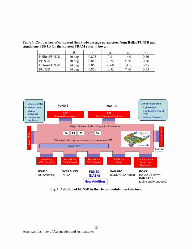
Computational Research and Engineering Acquisition Tools and Environments – Air Vehicles (CREATETM-AV) program and the US Army. A key highlight of the Helios framework architecture is its modular, flexible design, as depicted in Fig. 1. Modules of different disciplines communicate through a light-weight middleware written in the Python language. The modular design greatly facilitates new modules to be interfaced with Helios. This allows legacy, discipline-specific modules to be used within Helios, leveraging several years of development, validation, and user experience base.

One such instance is the NASA’s OVERFLOW flow solver [2,3], which was recently enhanced with an interface for Helios [4]. OVERFLOW offers high-order spatial accuracy, inherent speed and efficiency of structured grid solvers, and advanced turbulence models. The availability of OVERFLOW in addition to the existing NSU3D [5] unstructured near-body solver enabled simultaneous application of multiple near-body solvers to different rotorcraft components for efficient modeling of the rotorcraft, e.g., employ OVERFLOW for modeling the rotor blades, which are generally amenable to structured grids, and employ NSU3D for modeling hubs and fuselages, which tend to be geometrically complex and hence more suitable for unstructured grids. Moreover, the high numerical accuracy and efficiency in blade modeling directly improves performance and loads predictions and overall simulation efficiency. Helios interfaces are supported in OVERFLOW v2.2k and later and can be used in Helios v4.2 and later.

Success with use of OVERFLOW within Helios generated motivation for developing an interface for NASA’s FUN3D (Fully Unstructured Navier-Stokes) flow solver [6] as well. FUN3D is a state-of-the-art

H


3

general-unstructured grid flow solver and has been continuously developed, maintained, and supported by NASA Langley since late the 1980s. It has a broad user base within the US government, industry, and academia with applications in both fixed wing [7,8] and rotary wing [9,10] modeling. Additionally, it has a number of features that could be leveraged in Helios in the near future: (a) adjoint-based optimization and error estimation, (b) advanced turbulence and turbulence transition models, (c) ability to handle flows from incompressible to hypersonic regimes, including finite-rate chemical kinetics, (d) thermal radiation modeling, (e) active flow control modeling, and (f) generalized aero-elastic coupling.

The availability of FUN3D in Helios, on the other hand, allows FUN3D users to benefit from the multi-solver modular paradigm that has been successfully used within Helios for a number of applications [11–14]. Specifically, the ability to use FUN3D in combination with other HELIOS modules: (a) OVERFLOW, (b) SAMARC, a high-order automated adaptive Cartesian mesh solver module [15], (c) PUNDIT, a dynamic, automated, parallel domain connectivity module, (d) COVIZ, a parallel co-visualization module. The SAMARC code is composed of an adaptive mesh software from Lawrence Livermore National Lab, SAMRAI [15], and a high-order Cartesian version of the NASA Ames ARC3D code [3]. SAMARC solves the (inviscid) Euler equations using a fifth-order accurate spatial scheme and a third-order explicit Runge-Kutta time integration scheme. PUNDIT (Parallel Unsteady Domain Information Transfer) is the domain connectivity module that manages all aspects of overset mesh operations including hole-cutting, fringe points and solution stencil identification, solution interpolation, and data transfer. The overset mesh operations are performed in a fully automated fashion without any manual, mesh-specific inputs.

Most importantly, the integration of FUN3D in Helios, along with OVERFLOW, which was previously integrated, lays the ground for future interactions where capabilities of one component could be leveraged in others in a relatively seamless fashion. The strategies adopted for the integration are described in the next section, followed by validation studies.

Helios/FUN3D Integration The Helios framework has a defined set of interfaces for different modules. Since FUN3D is used only

as a near-body solver module in Helios, only the near-body solver interface procedures were implemented in FUN3D. FUN3D is not used to solve in the off-body regions; and instead, the adaptive Cartesian mesh generator and solver SAMARC is used. As noted before, all of the overset domain connectivity operations are performed using PUNDIT. PUNDIT obtains the grid coordinates and connectivity information from FUN3D and other solvers, such as OVERFLOW and SAMARC, and performs hole cutting and identifies the hole, fringe, orphan, and field points. During the simulation FUN3D sends the flow solution to PUNDIT, which performs the overset solution interpolation. This process is fully automated with no user inputs for static or dynamic cases involving multiple moving bodies.

Helios cases usually involve moving and deforming blades. The deformations are either prescribed or obtained from a Computational Structural Dynamics (CSD) solver. Hence the mesh needs to be moved/deformed at every time step. Helios offers a mesh motion module to perform the mesh update operations. However, FUN3D’s native mesh-motion functions were used instead as they are well integrated and validated with its flow solver. The mesh motion information is obtained from Helios and the FUN3D updates the mesh based on that information.

The Helios interface performs the following tasks: (1) Initialize – read native input files, read Helios inputs, set up FUN3D based on these inputs, allocate

memory for basic arrays, read and partition the mesh. (2) Get grid coordinates and connectivity – obtain grid coordinates, connectivity, and other overset data

for PUNDIT (3) Get/set flow solution – create flow solution data arrays for PUNDIT and update them during the

simulation. (4) Get surface loads – obtain the surface loading data for coupling with CSD solvers, and update them

during the simulation


4

(5) Set grid motion and update mesh – obtain grid motion data from Helios and move grid to the new position. The motion data includes both the rigid-body motions as well as the elastic deformations

(6) Solve for one step – advance the solution by one step (7) Write restart and plotting data – write output and restart files (8) Shut down – release system resources and stop the module The Helios interface was implemented where possible in FUN3D by overloading standard FUN3D

functions that perform similar tasks, such as overset grid assembly. The FUN3D Helios module registers the Helios specific implementations at startup and then follows the standard execution path whereby the registered implementation is called through an abstract interface. This eliminates the need to introduce logic into FUN3D to determine if it is executing in the Helios environment. The interfaces are supported in FUN3D v12.8 and later, and are compatible with Helios v4.2 and later. The Helios/FUN3D capability was validated for number of different test cases, each emphasizing certain unique aspects. These validation cases are presented in the following sections.

Validation Cases The Helios/FUN3D capability is validated for a number of cases that exercise most of the intended uses

of the FUN3D near-body solver. Validation was performed by comparing against the test data and/or the previous calculations using Helios and/or standalone FUN3D. The following validation cases were performed:

1. Tilt Rotor Aeroacoustic Model (TRAM) in hover 2. UH-60A isolated rotor in high-speed forward flight 3. Higher-harmonic Aeroacoustics Rotor Test (HART) II in low-speed descent 4. Counter-rotating dual rotors 5. Tandem-rotor H-47 full-aircraft

These cases are presented in the following sections.

Case I. TRAM in hover The first validation case is the hover performance prediction for the isolated TRAM rotor. A similar

validation study was also performed recently for the four-bladed S-76 isolated rotor with Helios/FUN3D in Ref. 23. TRAM is a model-scale rotor that is representative of tiltrotors. It was tested as an isolated rotor at the German-Dutch Wind Tunnel (DNW) [16]. It was designed to be a 1/4-scale version of the V-22 rotor. As with other tiltrotors, the rotor blades have a significantly greater amount of twist than a conventional helicopter rotor. The airfoils vary along the blade and are defined as XN28, XN18, XN12, and XN09 at radial locations 0.2544, 0.50, 0.75, and 1.00, respectively. The rotor solidity is 0.105, the tip Reynolds number, 𝑅𝑅𝑒𝑒𝛾𝛾, is 2.06 million, and the tip Mach number, 𝐹𝐹𝑡𝑡𝑡𝑡𝑡𝑡, is 0.62.

This case was selected with the objective to test/verify the following: 1. Setting up of FUN3D moving bodies from Helios motion inputs 2. Setting up of FUN3D rotor bodies from Helios rotor inputs 3. Domain connectivity and solution interpolation between FUN3D and SAMARC (off-body solver) The rotor blades were modeled as rigid (not as elastic, deforming structures). Also a fixed (no dynamic

grid adaption) off-body Cartesian mesh was used. Elastic structures and dynamic grid adaption were tested for the more advanced cases presented later in this paper. The validation metrics for the TRAM were the rotor performance and blade airloads.

The Helios/FUN3D mesh system is depicted in Fig. 2. The unstructured blade grids were solved using FUN3D, and the off-body Cartesian mesh was solved using SAMARC. The blade-grid cells farther away than one chord distance from the blade surface were removed through a grid-trimming procedure. The trimming reduces the rapid diffusion of the vortices. The blade mesh size is about 4.5 million nodes per blade. The off-body mesh cell size in the immediate vicinity of the blade is 5% chord (the L1 region in the figure) and is increased to 10% chord in the far-wake region (the L2 region in the figure) that starts from a distance of about 50% 𝑅𝑅 below the rotor. The off-body mesh size is about 156 million points.


5

The simulations were performed in time-accurate mode with a time step size of 0.25 deg. with 30 dual-time stepping subiterations within each time step. For the blades, a second-order spatial scheme based on Roe’s Flux Difference Splitting scheme with MUSCL (Monotone Upwind Scheme for Conservation Laws) variable extrapolation is used. The time advancement is based on the BDT2opt scheme available in FUN3D. The Spalart-Allmaras turbulence model [17] with Dacles-Mariani rotation correction [18,19] was used. The off-body Cartesian meshes were solved using SAMRAC. The wake was modeled as inviscid; and hence, viscous terms were not activated in this region. The inviscid terms used the fifth-order scheme (sixth-order central difference scheme with second-order and sixth-order dissipation terms). For time advancement, the third-order accurate explicit scheme was used.

The collective pitch angle, 𝜃𝜃𝛾𝛾, of the blade was varied from 6 to 16 deg. in the steps of 2 deg. For each collective angle the simulation was run for 20 revolutions to achieve convergence in the rotor thrust and torque. The computed rotor wake for the 14 deg. collective angle is shown in Fig. 3. A discrete tip vortex structure emanates from the wake and, due to the wake instability, quickly disintegrates into broken vortical structures. This has been reported in numerous previous investigations [20–24]. The computed figure of merit (FM) is compared in Fig. 4 with the test data and the predictions using the standalone FUN3D for 𝜃𝜃𝛾𝛾 = 10 and 14 deg. The standalone FUN3D computations were fully viscous for the near-body and off-body meshes with Spalart’s Delayed Detached Eddy Simulation (DDES) turbulence model [25]. The same blade mesh was used for the Helios/FUN3D and the FUN3D standalone computations. However, for the FUN3D standalone computations, the off-body mesh comprised of unstructured tetrahedral cells, and was much coarser, roughly 10% chord spacing in the vicinity of the blade, than the one used in Helios. Also the spatial accuracy in the off-body mesh was second-order compared to the fifth-order order scheme in Helios. Nevertheless, very close agreement was obtained between the standalone FUN3D and Helios/FUN3D predictions. The difference in FM predictions is less than 0.005. The agreement with the test data is also very good. The FM is under-predicted by about 0.01, which is quite acceptable given that the test data also has uncertainty of similar magnitude, in general. Also, the present calculations were made assuming fully-turbulent flow over the blades, whereas, in reality, the flow might be transitional at the model-scale Reynolds number of 2.06 million in the present case.

Helios/FUN3D blade section normal force, 𝐹𝐹2𝐶𝐶𝑁𝑁, predictions are compared with the test data and standalone FUN3D in Fig. 5 for 𝜃𝜃𝛾𝛾 = 10 and 14 deg. The blade vortex interaction (BVI) at the first blade passage is evident at around 90-95% 𝑅𝑅 where there is a bump in the radial variation of the normal force. The two predictions agree very well for the 10 deg. case. But for the 14 deg. case, the standalone FUN3D predicts a stronger BVI. The parameters characterizing with the first blade passage: (a) radial position, (b) axial position, (c) peak vorticity in the core, and (d) the core radius, were therefore compared between the two analyses, as presented in Table 1. The radial positions are consistent between the two predictions. However, the standalone FUN3D predicts a closer axial distance. Also, in the standalone FUN3D case, the vortex core radius is quite large and hence the vorticity in the core is much reduced due to a larger numerical diffusion of the vortex in the coarse, second-order accurate, unstructured off-body mesh. Therefore, a stronger BVI results both due to the closer axial distance as well as a larger core size. For the 14 deg. case the vortex is stronger and the axial distance is relatively much closer in standalone FUN3D case, which results in a stronger BVI. Besides the BVI loading, the two predictions agree very well at inboard locations. The agreement with the test data is fair.

Case II: UH-60A rotor in high-speed forward flight The second validation case is the isolated UH-60A rotor in high-speed forward flight. The UH-60A rotor

is a four-bladed fully articulated rotor. The rotor is composed of SC1095 and SC1094R8 airfoils. The rotor solidity, 𝜎𝜎, is 0.0826. The high-speed steady level flight condition, Counter 8534 (C8534), from the NASA/Army UH-60A Airloads Program (Ref. 26) is examined. The advance ratio, 𝜇𝜇, is 0.368 and the estimated blade loading, 𝐶𝐶𝑇𝑇/𝜎𝜎, is 0.084. This condition is characterized by transonic flow on the advancing side and high vibratory loads.

This case was selected as an extension to the first validation case to test/verify the following:


6

1. Forward flight 2. Blade elastic deformations data transfer from the Helios to FUN3D 3. Mesh deformation 4. Coupling with the CSD module to obtain trim and blade deformations RCAS was used for CSD modeling. The RCAS model of the rotor blade used 13 nonlinear beam

elements. The rotor hub was modeled as fully articulated with pitch bearing, and flap and lag hinges. For the rotor trimming procedure the measured rotor thrust, hub pitching, and hub rolling moments were specified as the trim targets; and collective pitch, longitudinal cyclic pitch, and lateral cyclic pitch were used as the trim variables. The shaft tilt of the rotor, 𝛼𝛼𝑠𝑠, was held fixed at -7.31 deg. The CFD-CSD exchange of the blade deformation and blade airloads used the “delta” loose-coupling formulation [21]. The CFD mesh system is similar to the one used for the previous case. The blade mesh size was about 1.1 million nodes per blade. The wake mesh had the finest spacing of 10% chord around the rotor and had about 9 million nodes.

The simulations were performed with a time step size of 0.25 deg. with 30 dual-time stepping subiterations within each time step. The standard Spalart-Allmaras model was used for turbulence modeling. As with the previous case, the off-body Cartesian meshes are modeled as inviscid.

The CFD-CSD exchange was performed every 90 deg., and the simulation was run for four revolutions. The computed wake is shown in Fig. 6. Due to the high forward speed and the forward shaft-tilt, the wake is quickly convected away from the rotor. After four revolutions, the blade airloads and deformations were well converged. The blade airloads are compared with the test data in Fig. 7. The predictions from Helios/OVERFLOW are also shown for reference. The two predictions are in excellent agreement with each other. The agreement with the test data is also good.

Case III: HART II rotor-fuselage in low-speed descent The next validation case builds upon the previous two cases and is targeted toward the modeling of

interactional aerodynamics of a rotor-fuselage configuration case and further validate the following: 1. Ability of the FUN3D module to manage motion data for cases involving combination of moving

(rotor blades) and non-moving (fuselage) bodies 2. Ability to accuracy predict the BVI loads and wake geometry for a case involving interactional

aerodynamics. HART II data was selected as it serves well the objectives of this validation. HART II campaign was

carried out in 2001 [27–29] in the German-Dutch wind tunnel (DNW). The test measurements include three-component Particle Image Velocimetry (3C-PIV), Stereo Pattern Recognition (SPR), noise measurements, blade surface pressure, and blade airloads. The rotor is a 40% Mach- and dynamically-scaled Bo105 hingeless rotor. It has four blades. The blade planform is rectangular and the blade airfoil section is NACA23012. The blade has a linear distribution of 8 deg. over the radius.

Of the several conditons tested, the baseline case is selected for the present study. The rotor speed, Ω, is 1,041 RPM, 𝐶𝐶𝑇𝑇/𝜎𝜎 is 0.056, 𝜇𝜇 is 0.15, and 𝛼𝛼𝑠𝑠 is 5.3 deg. However, 𝛼𝛼𝑠𝑠 in the computation model is set to 4.3 deg aft to account for the wind-tunnel wall correction. This flight condition simulates a slow descent with significant BVI interactions. The BVI induces unsteady, oscillatory loading on the rotor.

Accurate prediction of the BVI airloads is a challenging validation problem as both the strength and the position of the tip vortices must be accurately predicted. A number of CFD studies have been performed on the HART II rotor. Reference 30 summarizes predictions from a number of recent CFD-CSD studies performed using structured, unstructured, and hybrid CFD/Lagrangian-wake methods. In Ref. 31 a high resolution CFD study using CREATE-AV Helios is presented. In Ref. 31, the OVERFLOW near-body module was used for the blades. These Helios/OVERFLOW predictions and the test data are used here to validate the Helios/FUN3D predictions.

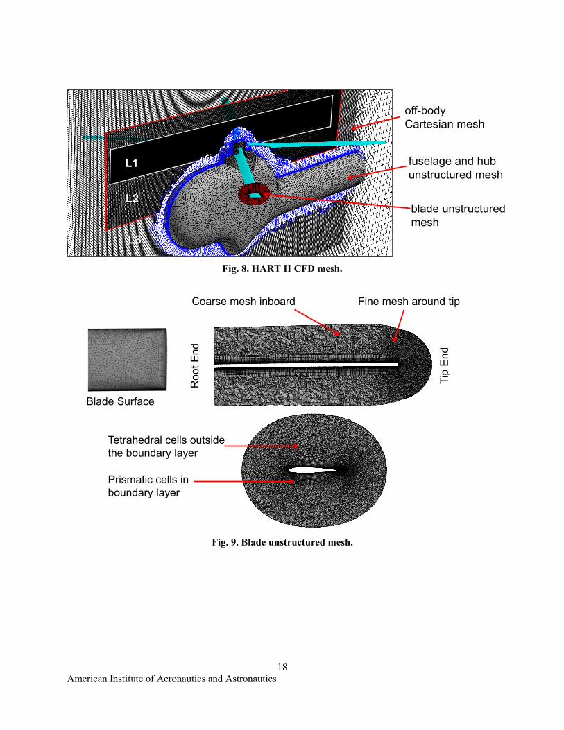
Unstructured meshes from Ref. 31 were used for the blades, fuselage and hub, and a Cartesian mesh is used in the rotor wake region. The mesh system is illustrated in Fig. 8. The blade mesh is shown in Fig. 9. The blade mesh has about 3.5 million nodes per blade. The hub and fuselage has about 0.8 million nodes.


7

A fine Cartesian mesh is used in the wake region. A uniformly fine mesh is used in the immediate vicinity of the rotor. As depicted in Fig. 8, the wake mesh is partitioned in three levels. The Level-1 (L1) region houses the immediate vicinity of the rotor plane. This region extends 4.5 chords above and below the rotor plane. The vortices from the blade mesh convect into this region first. Therefore, the mesh resolution is the finest in this region. A mesh spacing of 3.2% chord is used. Level-2 (L2) region houses the rotor L1 region. The mesh spacing is twice that of the L1 region or 6.4% chord. Level-3 (L3) region houses the regions L1 and L2 and the fuselage. The mesh spacing is twice that of the L2 region or 12.8% chord. The L3 region is rapidly coarsened and transitioned to the farfield boundaries. Total mesh size is about 739 million nodes.

The blades are modeled as elastic structures. The elastic deformations of the blade are prescribed via an input file. These blade deformations were obtained from a previous coupled CFD-CSD simulation reported in Ref. 32. The simulation was carried out for four rotor revolutions to achieve periodic convergence. The time step size of 0.1 deg. with 25 dual-time stepping subiterations within each time step was used for temporal convergence. For turbulence modeling, the standard Spalart-Allamas model was used. As with the previous cases, the off-body Cartesian meshes were modeled as inviscid. The computed wake structure, tip vortex vorticity and position, and blade airloads are presented in the following sections.

1. Rotor Wake Structure

The descent flight condition causes the rotor wake to stay in the close proximity to within a few chords of the rotor plane. The rotor wake at the rotor azimuth, 𝜓𝜓, of 70 deg. and 110 deg. are illustrated in Figs. 10 and 11, respectively. The figures show the schematic diagram, the computed wake from the Helios/OVERFLOW simulation [31], and the computed wake from the present Helio/FUN3D simulation. The two computed wake structures are very similar to each other and qualitatively matches closely to the schematic diagram.

As the advancing blade travels from 70 to 110 deg. azimuth, it interacts with the tip vortices and produces BVI airloads. Similarly, the BVI loads are also produced as retreating blade travel from 250 to 340 deg. azimuth. The blade on the front of the rotor disk interacts with the three tip vortices created during the previous three blade-passages. However, unlike the BVIs on the advancing and retreating sides, here the vortices are oriented perpendicular to the blade and their radial location remains relatively invariant with the blade azimuth, and therefore, little time variation occurs on the BVI loads. Finally, the blade on the aft of the rotor disk encounters large unsteady loading due to interaction with the root vortices and the hub wake (Figs. 10 and 11) but does not encounter BVIs.

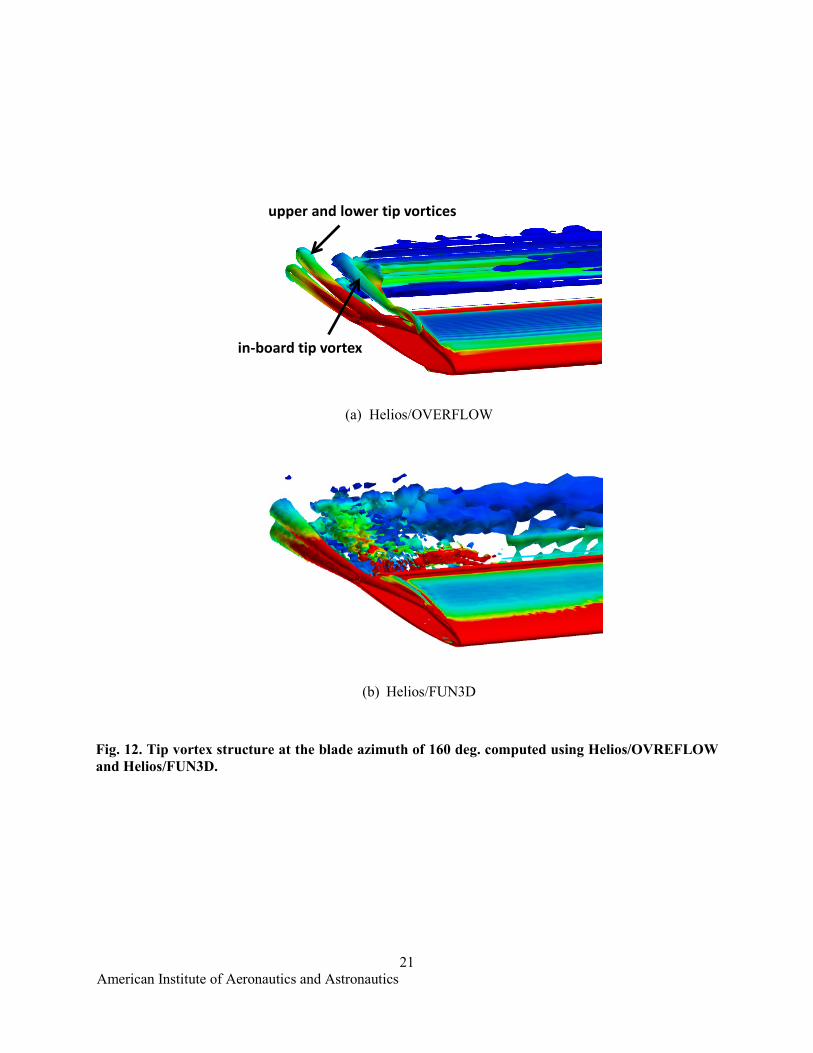
The tip vortex structure at the 160 deg. blade azimuth is shown in Fig. 12. The figure illustrates the outboard and inboard tip-vortex structure. The roll up from the blade lower and upper surfaces leads to two distinct vortex formation. In addition an inboard vortex structure also develops. This is clearly visible in the Helios/OVERFLOW simulation, which uses a much finer mesh compared to the one in Helios/FUN3D.

2. Tip Vortex Vorticity and Position

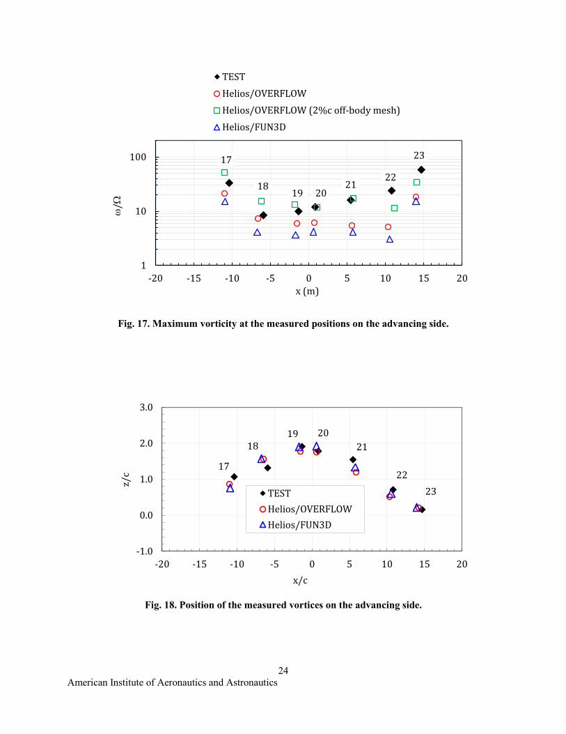
The test measurements of the position and strength were made at several longitudinal planes on the advancing and retreating sides as noted in Figs. 10 and 11. The measurement positions on the advancing side are marked 1–30, and on the retreating side are marked 31–53. Simulation results are compared against positions 17–23 on the advancing side longitudinal plane of 𝑦𝑦/𝑅𝑅 = 0.7, and positions 43–47 on the retreating side plane, at 𝑦𝑦/𝑅𝑅 = -0.7. Tip vortices on the advancing side positions are presented in Fig. 13, and positions 20, 21, 22, and 23 are presented in Fig. 14. The vortex structure computed using Helios/FUN3D is very similar to the one before using Helios/OVERFLOW. The vortex at position 17 is the newest vortex of all, and its wake age is about 25.3 deg. Subsequent vortices represent this vortex at later wake-ages: wake-age of vortex at positions 18, 19, 20, 21, 22, and 23 are 115.3, 205.3, 245.3, 335.3, 425.3, and 515.3 deg., respectively.

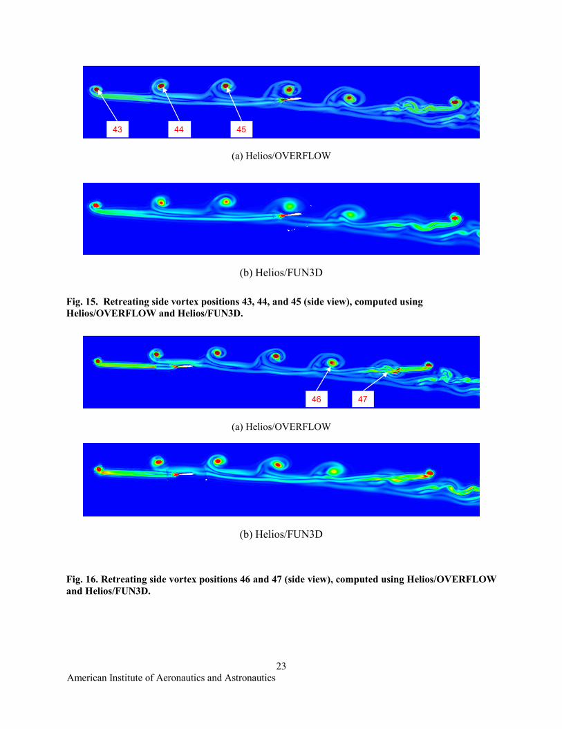
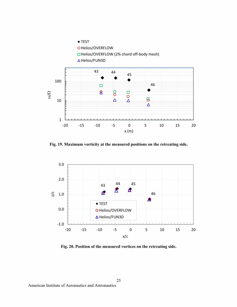
The tip vortices on the retreating side positions 43, 44, and 45, computed by CFD, are shown in Fig. 15, and positions 46 and 47 are shown in Fig. 16. Among these, the vortex at position 43 is the newest with


8

a wake-age of about 65 deg., and subsequent vortices represent the vortex at position 43 at later wake-ages: wake-age of vortex at positions 44, 45, 46, and 47 are 155, 245, 285, and 375 deg., respectively. Similar to the advancing side positions, the vortex structure computed using Helios/FUN3D and Helios/OVERFLOW are very similar.

Maximum vorticity (strength) and position of vortices 17–23 are compared against the test data in Figs. 17 and 18, respectively. The test measurements show that at position 17 the normalized vorticity, 𝜔𝜔, is about 34. The vorticity drops subsequently, but later, the strength at position 23 increases to about 60, which is contrary to the expectation that strength should continue to decay over the wake age. One possible explanation for the increase is that as the vortex at position 22 (wake-age = 425.3 deg.) travels down to position 23 (wake age = 515.3 deg.), it comes very close to the vortex convected from the preceding blade at 110 deg. azimuth, as depicted in Fig. 11. The test measurements, presumably, measure this new vortex and not the aged vortex that travels from position 22 to 23. Therefore, for consistency, the predictions at position 23 include the strength of this new vortex. The vorticity levels are largely underpredicted both with Helios/OVERFLOW and Helios/FUN3D. The underprediction is larger with Helios/FUN3D as the blade mesh is much coarser, causing a larger numerical diffusion. The vortex position is predicted very well in both results. Figure 17 also includes Helios/OVERFLOW results where a finer wake resolution of 2% chord was used. With a finer wake mesh, the vorticity levels are significantly better predicted. The vortex position is predicted very well.

Strength and position of vortices 43–47 on the retreating side are shown in Figs. 19 and 20, respectively. The test data shows that these vortices are much stronger compared to the vortices on the advancing side. The strongest vortex is at position 43 where the wake-age is about 65 deg. The test-measured strength (normalized vorticity) is about 150. Then the vorticity gradually decreases to about 35 at position 46 where the wake-age is about 285 deg. Both Helios/FUN3D and Helios/OVERFLOW results significantly underpredict the strength. Figure 19 also includes Helios/OVERFLOW results where a finer wake resolution of 2% chord was used. Unlike the advancing side, there is only a small increase the vorticity levels. The under prediction is larger with the Helios/FUN3D results due to the coarse blade mesh resolution and is consistent the advancing side correlations. The vortex position is predicted very well, slightly better then the prediction on the advancing side.

3. Blade Airloads

Finally, the airloads associated with BVIs are shown in Figs. 21 (a) and 22 (a) for the blade section normal force and pitching moment, respectively. The mean (steady component) has been removed from both the quantities to visualize the unsteady variations. As illustrated in Figs. 10 and 11, the advancing side blade interacts with eight tip vortices of decreasing wake-age as it moves from 0 to 100 deg. azimuth. Six of these vortices are encountered between 20 to 70 deg., and two are encountered from 70 to 100 deg. Correspondingly, six local peaks in normal force and pitching moment loadings are visible in the test data between 20 to 70 deg. azimuth, and are captured very well both in the Helios/FUN3D as well as Helios/OVERFLOW results. The BVI loading can be more clearly seen when only the higher harmonics of the loads are plotted. Figures 21 (b) and 22 (b) show the higher harmonic components of sectional normal force and pitching moment, respectively. The six loading peaks between 20 and 70 deg. are clearly shown in the test data. Both simulation results captures all the peaks with a good correlation in phase and a fair correlation in magnitude. The pitching moment shows an extra peak at around 30 deg. in the Helios/OVERFLOW results, which seems to be due to the interactions with the inboard tip vortex shown in Fig. 11. This peak seems to be present in the Helios/FUN3D results as well, but it is quite diffused. A close-up view of the tip vortex is illustrated in Fig. 12.

The retreating side blade interacts with five tip vortices of increasing wake-age as it moves from 250 to 360 deg. azimuth, as shown in Figs. 10 and 11. Correspondingly, the test data shows the five peaks in the blade section normal force and the blade section pitching moment higher harmonic loadings shown in 21 (c) and and 22 (c), respectively. Both the Helios/OVERFLOW and Helios/FUN3D results capture both the phase and magnitude of the normal force and the pitching moment very well.


9

Case IV: Counter-rotating dual rotors The next case involves a more complex dual-rotor case with the objective of testing the following

features: 1. Ability to model counter-rotating dual rotors with elastic blades 2. Ability to simulate change in aircraft attitude with grid speeds provided by Helios These tests were performed primarily as a prerequisite to performing the full aircraft steady free-flight

trim calculation of the tandem-rotor H-47 calculation presented in the next section. For the purposes of verification, a fictitious dual, counter-rotating rotors configuration was created from the UH-60A isolated rotor case presented before. Rotors were separated far enough to avoid any mutual aerodynamic interference. The rotor blades were modeled as elastic structures. The elastic deformation of the blades was prescribed via motion files from the converged CFD-CSD solution obtained from Case III.

Helios allows the aircraft attitude to be simulated via grid speeds instead of physically orienting the mesh. To verify that this feature works with Helios/FUN3D, the aircraft attitude was set to -2 deg., the hub pre-tilt angle (𝛼𝛼𝑠𝑠) was set to -3 deg., and the freestream angle-of-attack was set to -2.31 deg. This is equivalent to an angle of attack -7.31 deg. that was used in Case III. The computed airloads (not shown) from the two rotors were nearly-identical to the airloads presented in Fig. 7.

Case V: Tandem-rotor H-47 full-aircraft The final test case showcases the ability to model a complex full aircraft in steady free-flight trim. The

objective was to test and verify the following features: 1. Modeling of the full aircraft with a combination of different near-body solvers 2. CFD-CSD coupling for dual rotors 3. Free-flight trim 4. Adaptive Cartesian mesh The tandem-rotor H-47 full-aircraft model, with modeling of both the front and aft rotors, was used for

this study. A similar but more detailed study focused on rotor structural loads prediction using Helios will be presented at an upcoming paper (Ref. 33). In that study, the rotor blades are modeled using the OVERFLOW module, the hub and fuselage are modeled using NSU3D module, and the wake is modeled using SAMARC. In the present study the FUN3D module is used instead of NSU3D. The mesh system is depicted in Fig. 24 (a). The rotor structural dynamics were modeled using RCAS. The CFD-CSD coupling was carried out every period (120 deg. of rotation for the three-bladed rotors) until convergence/periodic solution was reached. A free-flight trim procedure was carried out where the trim targets were the three forces and the three moments acting on the full rotorcraft. The trim targets were driven to zero by the trimming procedure. Even though the fuselage was modeled in the CFD simulation, a look up table was used within RCAS to obtain the fuselage forces and moments for trim calculation instead of using the ones computed by CFD. In this way, the rotor/fuselage interactions are captured accurately in CFD, while CSD is using a table lookup for fuselage contribution to trim. In the CFD simulations, the change in fuselage attitude was simulated by imposing equivalent translational grid speeds in the solvers without physically moving the grids.

The CFD-CSD coupling was carried out for four rotor revolutions, and a converged solution was obtained. The computed wake for a high-speed forward condition is shown in Figs. 24 (b)–(d). At the high speed the aircraft tilts forward to generate the propulsive force from the rotors. The forward tilt is simulated by imposing equivalent grid speeds, and hence, the wake is seen to convect downward. The trim state has a small sideslip angle, which causes the wake to drift sideways.

Summary and Concluding Remarks The NASA Langley FUN3D solver has been modularized and validated as a near-body solver for the

the CREATE-AVTM Helios software. To demonstrate that the two software have been sucessfully integrated, a series of key validation and verification cases were presented, each addressing unique validation metrics. The following cases were studied: (I) isolated TRAM rotor in hover for performance


10

and airloads; (II) isolated UH-60A rotor in high-speed forward flight for airloads and CFD/CSD coupling; (III) HART II rotor-fuselage for BVI loads, wake predictions, and combined rotor-fuselage modeling; (IV) dual counter-rotating UH-60A rotors for airloads and grid speed implementation; and finally, (V) tandem rotor H-47 full aircraft for multiple near-body solvers, CFD/CSD coupling for dual counter-rotating rotors, and free-flight trim with accounting for the fuselage aerodynamics loads.

Helios interfaces described here are supported in FUN3D v12.8 and later, and are compatible with Helios v4.2 and later. The integration of FUN3D in Helios, along with OVERFLOW, which was previously integrated in Helios, lays the ground for future interaction opportunities where capabilities of one component could be leveraged with others available in Helios in a relatively seamless fashion.

Acknowledgments The authors would like to acknowledge the support of the HART II partners from AFDD, DLR, DNW,

NASA, and ONERA.

References 1 Wissink, A.M., Sankaran V., Jayaraman B., Datta A., Sitaraman, J., Potsdam M., Kamkar S., Mavriplis

D., Yang Z., Jain R., Lim J., and Strawn, R., “Capability Enhancements in Version 3 of the Helios High-Fidelity Rotorcraft Simulation Code,” AIAA-2012-0713, AIAA 50th Aerospace Sciences Meeting, January 2012, Nashville, TN.

2 Nichols, R.H., Tramel R.W., and Buning, P.G., “Solver and Turbulence Model Upgrades to OVERFLOW 2 for Unsteady and High-Speed Applications,” AIAA-Paper 2006-2824, 24th AIAA Applied Aerodynamics Conference, San Francisco, CA, 5–8 June 2006.

3 Pulliam, T.H., “High Order Accurate Finite-Difference Methods: as seen in OVERFLOW,” AIAA-2011-3851, 20th AIAA Computational Fluid Dynamics Conference, Honolulu, HI, 27–30 June, 2011.

4 Jain, R. and Potsdam, M., “Strategies for OVERFLOW Modularization and Integration in Helios,” 11th Overset Grid Symposium, October 15-18 2012, Dayton, OH.

5 Mavriplis D.J., “NSU3D User’s Manual, Version 3.4 Rev 2,” Scientific Simulations, Yorktown, VA, September 2000.

6 Biedron, R. T., Carlson, J., Derlaga, J.M., Gnoffo, P.A., Hammond, D.P., Jones, W.T., Kleb B., Lee-Rausch, E.M., Nielsen E.J., Park, M.A., Rumsey, C.L., Thomas, J.L., and Wood, W.A., “FUN3D Manual: 12.7,” NASA TM-2015-218761, May 2015.

7 Park M.A., Laflin, K.R., Chaffin, M.S., Powell, N., and Levy, D.W., “CFL3D, FUN3D, and NSU3D Contributions to the Fifth Drag Prediction Workshop,” Journal of Aircraft, 2014, Vol. 51: 1268-1283, 10.2514/1.C032613.

8 Lee-Rausch, E.M., Rumsey, C.L., and Park, M.A., “Grid-Adapted FUN3D Computations for the Second High-Lift Prediction Workshop,” Journal of Aircraft, 2015, Vol. 52: 1098-1111, 10.2514/1.C033192.

9 Lee-Rausch, E.M. and Biedron, R.T., “FUN3D Airload Predictions for the Full-Scale UH-60A Airloads Rotor in a Wind Tunnel,” AHS 69th Annual Forum, Phoenix, AZ, May 2013.

10 Smith, M.J., Lim, J.W., Wall, B.G., Baeder, J.D., Biedron, R.T., Boyd, D.D., Jayaraman, B., Jung, S. N., and Min, B. Y., “The HART II International Workshop: An Assessment of the State-of-the-Art in CFD/CSD Prediction,” CEAS Aeronautical Journal, Vol. 4, (4), 2013, pp. 345–372.

11 Jain, R. and Potsdam, M., “Hover Predictions on the Sikorsky S-76 Rotor using Helios,” AIAA 2014-0207, AIAA Science and Technology Forum and Exposition (SciTech2014), 13–17 January 2014, National Harbor, MD.

12 Jain, R., “Hover Predictions for the S-76 Rotor with Tip Shape Variation using CREATE-AV Helios,” AIAA 2015-1244, AIAA Science and Technology Forum and Exposition (SciTech2015), 5–9 January 2015, Kissimmee, Florida.

http://arc.aiaa.org/author/Park%2C+Michael+A

http://arc.aiaa.org/author/Laflin%2C+Kelly+R

http://arc.aiaa.org/author/Chaffin%2C+Mark+S

http://arc.aiaa.org/author/Powell%2C+Nicholas

http://arc.aiaa.org/author/Levy%2C+David+W

http://arc.aiaa.org/loi/ja

http://arc.aiaa.org/author/Rumsey%2C+C+L

http://arc.aiaa.org/author/Park%2C+M+A

http://arc.aiaa.org/loi/ja

http://fun3d.larc.nasa.gov/chapter-2.html#rausch_ahs2013

http://fun3d.larc.nasa.gov/chapter-2.html#rausch_ahs2013


11

13 Jain, R., Joon W.L., and Jayaraman, B., “Helios Modular Multi-solver Approach for Efficient High-fidelity Simulation of the HART II Rotor,” Fifth Decennial American Helicopter Society Aeromechanics Specialists' Conference, Jan 22-24, 2014, San Francisco, California.

14 Potsdam, M., and Jayaraman, B., “UH-60A Rotor Tip Vortex Prediction and Comparison to Full-Scale Wind Tunnel Measurements,” AHS 70th Annual Forum and Technology Display, Montréal, Québec, Canada, May 22-24, 2014.

15 Hornung, R.D., Wissink, A.M., and Kohn, S.R., “Managing Complex Data and Geometry in Parallel Structured AMR Applications,” Engineering with Computers, Vol. 22, (3-4), 2006, pp. 181–195.

16 Young, L.A., Booth, E.R., Jr., Yamauchi, G.K., Botha, G., and Dawson, S., “Overview of the Testing of a Small-Scale Proprotor,” American Helicopter Society 55th Annual Forum, Montréal, Canada, May 25–27, 1999.

17 Spalart, P.R. and Allmaras, S.R., “A One-Equation Turbulence Model for Aerodynamic Flows,” La Recherche Aerospatiale, Vol. 1, No. 1, 1994, pp. 5–21.

18 Dacles-Mariani, J., Zilliac, G.G., Chow, J.S., and Bradshaw, P., “Numerical/Experimental Study of a Wingtip Vortex in the Near Field,” AIAA Journal, Vol. 33, No. 9, Sept. 1995, pp. 1561–1568.

19 Dacles-Mariani, J., Kwak, D., and Zilliac, G., “On Numerical Errors and Turbulence Modeling in Tip Vortex Flow Prediction,” International Journal for Numerical Methods in Fluids, Vol. 30, No. 1, 1999, pp. 65–82.

20 Chaderjian, N.M. and Buning, P. G., “High Resolution Navier-Stokes Simulation of Rotor Wakes,” Proceedings of the 67th Annual Forum of the American Helicopter Society, Virginia Beach, VA, May 2011.

21 Potsdam, M., Yeo, H., and Johnson, W., “Rotor Airloads Prediction Using Loose Aerodynamic/ Structural Coupling,” Journal of Aircraft, Vol. 43, (3), May-June 2006, pp. 732-742.

22 Hariharan, N., Potsdam, M., and Wissink, A., “Helicopter Rotor Aerodynamic Modeling in Hover Based on First-Principles: State-of-the-Art and Remaining Challenges,” 50th AIAA Aerospace Sciences Meeting including the New Horizons Forum and Aerospace Exposition, January 9–12 2012, Nashville, TN, AIAA 2012-1066, DOI: 10.2514/6.2012-1066.

23 Jain, R., “A CFD Sensitivity Study of Hover Performance Prediction Using HPCMP CREATE-AV Helios,” Abstract accepted for the AIAA Science and Technology Forum and Exposition (SciTech2016), January 4–8 2016, San Diego, California.

24 Chaderjian, N.M., and Ahmad, J. U., “Detached Eddy Simulation of the UH-60 Rotor Wake Using Adaptive Mesh Refinement,” Proceedings of the 68th Annual Forum of the American Helicopter Society, Forth Worth, TX, May 2012.

25 Spalart, P.R., Deck, S., Shur, M.L., Squires, K.D., Strelets, M.K., and Travin, A., “A New Version of Detached-Eddy Simulation, Resistant to Ambiguous Grid Densities,” Theoretical and Computational Fluid Dynamics, Vol. 20, No. 3, 2006, pp. 181–195.

26 Kufeld, R.M., Balough, D.L., Cross, J.L., Studebaker, K.F., Jennison, C.D., and Bousman, W.G., “Flight Testing of the UH60A Airloads Aircraft,” American Helicopter Society 50th Annual Forum, Washington, DC, May 11–13, 1994.

27 Yu, Y.H., Tung, C., van der Wall, B.G., Pausder, H., Burley, C., Brooks, T., Beaumier, P., Delrieux, Y., Mercker, E., and Pengel, K., “The HART-II Test: Rotor Wakes and Aeroacoustics with Higher-Harmonic Pitch Control (HHC) Inputs-The Joint German/French/Dutch/US Project,” American Helicopter Society 58th Annual Forum Proceedings, Montreal, Canada, June 11–13, 2002.

28 Lim, J.W., Tung, C., Yu, Y.H., Burley, C. L., Brooks, T.F., Boyd, D., van der Wall, B. G., Schneider, O., Richard, H., Raffel, M., Beaumier, P., Delrieux, Y., Pengel, K., and Mercker, E., “HART II: Prediction of Blade-Vortex Interaction Loading,” 29th European Rotorcraft Forum Proceedings, Friedrichshafen, Germany, September 16–18, 2003.

29 van der Wall, B.G., “2nd HHC Aeroacoustics Rotor Test (HART II) – Part I: Test Documentation,” DLR IB 111-2003/19, Braunschweig, Germany, November 2003.


12

30 Smith, M.J., Lim, J.W., Wall, B.G., Baeder, J.D., Biedron, R.T., Boyd, D.D., Jayaraman, B., Jung, S.N., and Min, B.Y., “The HART II International Workshop: An Assessment of the State-of-the-Art in CFD/CSD Prediction,” CEAS Aeronautical Journal, 2013, Vol. 4, No. 4, pp. 345–372.

31 Jain, R., Lim, J., and Jayaraman, B., “Modular Multisolver Approach for Efficient High-Fidelity Simulation of the HART II Rotor,” Journal of the American Helicopter Society, Vol. 60, (3), July 2015.

32 Lim, J., and Dimanlig, A., "The Effect of Fuselage and Rotor Hub on Blade-Vortex Interaction Airloads and Rotor Wakes," 36th European Rotorcraft Forum Proceedings, Paris, France, September 7–9, 2010.

33 Meadowcroft, E.T. and Jain, R., “Improvements to Tandem-Rotor H-47 Helicopter Coupled CFD-CSD Full Aircraft Model,” Abstract submitted to the American Helicopter Society 72nd Annual Forum, West Palm Beach, FL, May 2016.


13

Table 1. Comparison of computed first blade passage parameters from Helios/FUN3D and standalone FUN3D for the isolated TRAM rotor in hover.

𝜃𝜃𝛾𝛾 𝑟𝑟 𝑧𝑧 𝜔𝜔 𝑟𝑟𝛾𝛾 Helios/FUN3D 10 deg. 0.875 -0.31 16.0 0.26 FUN3D 10 deg. 0.880 -0.24 5.60 0.86 Helios/FUN3D 14 deg. 0.860 -0.68 31.5 0.25 FUN3D 14 deg. 0.860 -0.53 7.90 0.95

Fig. 1. Addition of FUN3D in the Helios modular architecture.

Object Oriented Python Integration Framework

DCFDomain Connectivity

FSIFluid Structure Interface

Distributed Memory processors communicating via MPI

shared data

P0 P1 P2 PN

PUNDIT Rotor FSI

NSU3D(U. Wyoming)

Off-Body Solver

Mes

h M

otio

n

SAMARC(LLNL/NASA Ames)

Near-Body CFD Solver-2


Co-

visu

aliz

atio

n

ParaviewFieldview

FUN3D(NASA)

Computational Structural Dynamics

RCAS (AFDD US Army)CAMRADII(Johnson Aeronautics)

• Object Oriented• Multiple codes• Multiple

languages• Generalized

Interfaces

Main execution script• Light-Weight• Few hundred lines of

code• Minimal Overheads

off-body

near-body

OVERFLOW(NASA)


New Addition


14

Fig. 2. Near-body and off-body grids for the TRAM rotor.

Fig. 3. Computed wake for the TRAM rotor using Helios/FUN3D.

blade unstructured mesh

spacing = 10 %c

Cartesian adaptive mesh

spacing = 5 %c


15

(a) Figure of merit

(a) Thrust versus collective

Fig. 4. Isolated TRAM rotor hover performance.

0.60

0.65

0.70

0.75

0.80

0.005 0.01 0.015 0.02

Exp

FUN3D

Helios/FUN3D

FM

CT

0.005

0.010

0.015

0.020

0 5 10 15 20

Exp

FUN3D

Helios/FUN3D

CT

Collective, deg.


16

Fig. 5. Isolated TRAM rotor blade section normal force (𝑴𝑴𝟐𝟐𝑪𝑪𝑵𝑵) in hover.

Fig. 6. UH-60A C8534 Isolated Rotor: Computed Wake

0

0.05

0.1

0.15

0.2

0.25

0.3

0 0.1 0.2 0.3 0.4 0.5 0.6 0.7 0.8 0.9 1

TEST, CT = 0.0110TEST, CT = 0.0149FUN3D CT = 0.0110FUN3D CT = 0.0154HELIOS/FUN3D, CT = 0.0108HELIOS/FUN3D, CT = 0.0152

r/R

M2 C

N


17

(a) 𝐹𝐹2𝐶𝐶𝑁𝑁, 86.5% 𝑅𝑅

(b) 𝐹𝐹2𝐶𝐶𝑀𝑀, 86.5% 𝑅𝑅 (mean removed)

(c) 𝐹𝐹2𝐶𝐶𝑁𝑁, 96.5% 𝑅𝑅

(d) 𝐹𝐹2𝐶𝐶𝑀𝑀, 96.5% 𝑅𝑅 (mean removed)

Fig. 7. UH-60A rotor blade airloads from CSD-CSD coupling for the high-speed case (C8534).

-0.20

-0.10

0.00

0.10

0.20

0.30

0 60 120 180 240 300 360

TestHelios/OVERFLOWHelios/FUN3D

ψ

-0.020

-0.015

-0.010

-0.005

0.000

0.005

0.010

0.015

0 60 120 180 240 300 360ψ

-0.15

-0.10

-0.05

0.00

0.05

0.10

0.15

0.20

0.25

0 60 120 180 240 300 360ψ

-0.025

-0.020

-0.015

-0.010

-0.005

0.000

0.005

0.010

0.015

0 60 120 180 240 300 360ψ


18

Fig. 8. HART II CFD mesh.

Fig. 9. Blade unstructured mesh.

L1

L2

L3

off-body Cartesian mesh

blade unstructured mesh

fuselage and hub unstructured mesh

Coarse mesh inboard Fine mesh around tip

Roo

t End

Tip

End

Prismatic cells inboundary layer

Tetrahedral cells outside the boundary layer

Blade Surface


19

Fig. 10. Rotor wake at 70 deg. rotor azimuth: (a) Schematic, (b) CFD wake computed using Helios/OVERFLOW, and (c) CFD wake computed using Helios/FUN3D. The isosurfaces of the Q-criterion at 0.0001 (colored by vorticity magnitude) are shown for the CFD wakes.

46 47

191817

y/R = 0.7

y/R = -0.7

Hub wake + Root Vortices

y

x

ψ

(b) Helios/OVERFLOW(a) Schematic

(c) Helios/FUN3D


20

Fig. 11. Rotor wake at 110 deg. rotor azimuth: (a) Schematic, (b) CFD wake computed using Helios/OVERFLOW, and (c) CFD wake computed using Helios/FUN3D. The isosurfaces of the Q-criterion at 0.0001 (colored by vorticity magnitude) are shown for the CFD wakes.

43 44 45

23222120

Hub wake + Root Vortices

Inboard tip vorticesy/R = 0.7

y/R = -0.7

y

x

ψ

(b) Helios/OVERFLOW(a) Schematic

(c) Helios/FUN3D


21

(a) Helios/OVERFLOW

(b) Helios/FUN3D

Fig. 12. Tip vortex structure at the blade azimuth of 160 deg. computed using Helios/OVREFLOW and Helios/FUN3D.

upper and lower tip vortices

in-board tip vortex


22

(a) Helios/OVERFLOW

(b) Helios/FUN3D

Fig. 13. Advancing side vortex positions 17, 18, and 19 (side view), computed using Helios/OVERFLOW and Helios/FUN3D.

(a) Helios/OVERFLOW

(b) Helios/FUN3D

Fig. 14. Advancing side vortex positions 20, 21, 22, and 23 (side view), computed using Helios/OVERFLOW and Helios/FUN3D.

191817

23222120


23

(a) Helios/OVERFLOW

(b) Helios/FUN3D

Fig. 15. Retreating side vortex positions 43, 44, and 45 (side view), computed using Helios/OVERFLOW and Helios/FUN3D.

(a) Helios/OVERFLOW

(b) Helios/FUN3D

Fig. 16. Retreating side vortex positions 46 and 47 (side view), computed using Helios/OVERFLOW and Helios/FUN3D.

43 44 45

46 47


24

Fig. 17. Maximum vorticity at the measured positions on the advancing side.

Fig. 18. Position of the measured vortices on the advancing side.

1

10

100

-20 -15 -10 -5 0 5 10 15 20

ω/Ω

x (m)

TESTHelios/OVERFLOWHelios/OVERFLOW (2%c off-body mesh)Helios/FUN3D

17

1819 20

2122

23

-1.0

0.0

1.0

2.0

3.0

-20 -15 -10 -5 0 5 10 15 20

z/c

x/c

TESTHelios/OVERFLOWHelios/FUN3D

17

19 2021

2223

18


25

Fig. 19. Maximum vorticity at the measured positions on the retreating side.

Fig. 20. Position of the measured vortices on the retreating side.

1

10

100

-20 -15 -10 -5 0 5 10 15 20

ω/Ω

x (m)

TESTHelios/OVERFLOWHelios/OVERFLOW (2% chord off-body mesh)Helios/FUN3D

43 44 45

46

-1.0

0.0

1.0

2.0

3.0

-20 -15 -10 -5 0 5 10 15 20

z/c

x/c


43 45

46

44


26

(a) Azimuthal variation (all harmonics), mean removed

(b) Higher harmonics (11–64/rev) on the advancing side

(c) Higher harmonics (11–64/rev) on the retreating side

Fig. 21. Normal force (M2CN) at 87%R span.

-0.05

-0.025

0

0.025

0.05

0 60 120 180 240 300 360


ψ

M2CN

-0.015

-0.005

0.005

0.015

10 20 30 40 50 60 70

M2CN

ψ

-0.025-0.015-0.0050.0050.0150.0250.035

250 270 290 310 330 350

M2CN

ψ


27

(a) Azimuthal variation (all harmonics), mean removed

(b) Higher harmonics (11–64/rev) on the advancing side

(c) Higher harmonics (11–64/rev) on the retreating side

Fig. 22. Pitching moment (M2CM) 87%R span.

-0.003

-0.002

-0.001

0

0.001

0.002

0 60 120 180 240 300 360


ψ

M2CM

-0.0015-0.001

-0.00050

0.00050.001

0.0015

10 30 50 70

M2CM

ψ

-0.0015-0.001

-0.0005-1E-170.0005

0.0010.0015

250 270 290 310 330 350

M2CM

ψ


28

(a) Front view

(b) Top view

Fig. 23. Helios/FUN3D verification of a multi-rotor case using two far-separated rotors. The shaft angle is -7.31 deg. but, for verification purposes, it is specified as a combination of a -3 deg. shaft-tilt, a -2.31 deg. freestream angle of attack, and -2 deg. of the aircraft pitch attitude which is simulated by imposing equivalent grid speeds.

Shaft pre-tilt

Freestream angle-of-attack =

Aircraft pitch attitude

Effective angle-of-attack =

Freestream


29

(a) Helios mesh system

(b) Downward convection of the wake due to aircraft pitch

(c) Sideward convection of the wake due to sideslip

(d) Front view

Fig. 24. CH-47 rotor-fuselage in forward flight. Blades are modeled using OVERFLOW, fuselage using FUN3D, and the wake region using SAMARC. Free-flight CFD-CSD calculations are performed using RCAS for CSD modeling.

off-body Adaptive Cartesian mesh(SAMARC)

blade structured mesh (OVERFLOW)

fuselage and hub unstructured mesh(FUN3D)

modularization and validation of fun3d as a create · pdf fileamerican institute of...

Documents