modis observed impacts of intensive agriculture on surface temperature in the southern great plains

INTERNATIONAL JOURNAL OF CLIMATOLOGYInt. J. Climatol. 30: 1994–2003 (2010)Published online 4 February 2010 in Wiley Online Library(wileyonlinelibrary.com) DOI: 10.1002/joc.2093

MODIS observed impacts of intensive agriculture on surfacetemperature in the southern Great Plains

Jianjun Ge*Department of Geography, Oklahoma State University, 337 Murray Hall, Stillwater, OK 74078 4073, USA

ABSTRACT: Land use/cover change has been recognized as an important component in regional and global climate.This study provides satellite observed impacts of agricultural activities on near surface climate. Land surface temperatureproducts from NASA’s earth observing system (EOS) Terra and Aqua satellites are used. The intensive winter wheat fieldin the southern Great Plains greatly modifies the seasonal, diurnal and spatial characteristics of surface temperature. Overthe period from August 2002 to July 2008, in terms of maximum daytime temperature the winter wheat field is 2.30 °Ccooler than surrounding grasslands in the growing season, but 1.61 °C warmer after its harvest. The maximum cool andwarm anomalies reach 4.16 °C and 3.35 °C, respectively. At night, the impacts of the wheat fields are less significantespecially after harvest. Spatially, the wheat field has more uniform surface temperature than grassland. Over the 6-yearperiod, the standard deviation of daytime land surface temperature over the wheat field is 0.72 °C smaller than grassland.The value of EOS observations for the land/climate interaction research is demonstrated, and similar analysis has potentialto be applied to other land use/cover changes in different regions. Copyright 2010 Royal Meteorological Society

KEY WORDS MODIS; land surface temperature; climate; agriculture

Received 26 November 2008; Revised 9 November 2009; Accepted 28 December 2009

1. Introduction

Land surface processes impact regional to global climateprocesses by controlling exchanges of mass, energyand momentum between ecosystems and atmosphere(Pielke et al., 2002). Much of the world’s land surfacehas been cleared for agriculture or human settlements.Together, croplands and pastures occupy nearly 40% ofthe continental surfaces, becoming one of the largestterrestrial biomes on the planet (Foley et al., 2005).Over the past decades, interactions between the landand atmosphere have been widely investigated (Xue,1997; Betts, 2000; Feddema et al., 2005; Ge et al.,2007), and the importance of anthropogenic land coverchange in global and regional climate change has receivedincreasing attention (Turner et al., 2007).

Agriculture-related land cover conversions have a sig-nificant impact on surface biophysical characteristics,surface energy partitioning and climate (Boucher et al.,2004; Pielke et al., 2007a). Conversion of natural ecosys-tems to farmland alters the surface roughness of vege-tation, albedo, leaf conductance and soil moisture. Anincrease in surface wetness due to irrigation increasesphysical evaporation and transpiration while decreasingsensible heat flux leading to a cooling of the surface.Additional moisture flux in the atmosphere will releaselatent heat and thus enhance the moist static energy within

* Correspondence to: Jianjun Ge, Department of Geography, OklahomaState University, 337 Murray Hall, Stillwater, OK 74078 4073, USA.E-mail: [email protected]

the convective boundary layer and consequently affectconvection and precipitation. Water vapour due to irriga-tion may also contribute to additional greenhouse effectand absorption of solar radiation.

Previous assessments of agricultural impacts onweather and climate have included both modelling andobservational studies. Segal et al. (1998), for example,used a mesoscale model to simulate the impacts of irriga-tion in North America on summer rainfall and suggestedan increase tendency of continental-average rainfall. Mar-shall et al. (2004) simulated the impacts of land covertransformation on the Florida Peninsula primarily due tolarge-scale agricultural production during the 20th cen-tury and found decreased precipitation and amplified diur-nal cycle of 2-m air temperature. Roy et al. (2007) used aregional model and observational datasets to investigatethe impacts of the Green Revolution-induced extensiveirrigation in India and showed that irrigation can substan-tially reduce air temperature during the growing season.At the global scale, Boucher et al. (2004) found a largesurface cooling of up to 0.8 K over irrigated land areasbut estimated a global mean radiative forcing in the rangeof 0.03–0.1 Wm−2 due to the increase in water vapourfrom irrigation. General circulation models (GCMs) usedto project climate response to increased CO2 generallyomit irrigation of agricultural land. A recent study byLobell et al. (2006) suggested potential bias of modelprojected greenhouse warming in irrigated regions inGCMs as GCMs generally omit irrigation of agriculturalland.

Copyright 2010 Royal Meteorological Society

AGRICULTURAL IMPACTS ON CLIMATE BY MODIS 1995

The evidence of the role of intensive agriculture inmodifying surface climate has also been documented byvarious observational studies. For example, Moore andRojstaczer (2002) found that irrigation enhanced precip-itation downwind in Texas High Plains, yielding stormsof greater duration, length and accumulation. Using dailyrainfall observations and monthly satellite land surfacedatasets, Niyogi et al. (2010) found that agriculturalintensification could be associated with reduced summermonsoon rainfall over certain regions of India. McPher-son et al. (2004) investigated the impacts of the winterwheat belt in Oklahoma and found a well-defined coolanomaly across the wheat belt during the growing sea-son and a warm anomaly after the wheat is harvested.Mahmood et al. (2006) examined the irrigation effectson near surface temperature of the northern Great Plainsusing long-term air temperature data from five irrigatedand five non-irrigated sites and found notably cooler tem-perature over irrigated areas. A recent empirical studyreported a significantly local cooling effect (−0.3 °C perdecade) due to change in surface albedo caused by inten-sive greenhouse horticulture in southeastern Spain (Cam-pra et al., 2008). This may have masked local warmingsignals associated to greenhouse gas increase.

Observation data in such studies are commonlyobtained from in situ point sources. Unfortunately, thesestations are neither located evenly nor densely; thus giv-ing an inadequate spatial representation over many areas.Limited number of stations selected for farming or non-farming areas can be influenced by many other factors,for example, changes in instrumentation, elevation, lati-tude and distance from water body (Bonfils and Lobell,2007). Furthermore, in situ stations are often interpolatedinto data-sparse regions. However, interpolation tends notto provide much additional independent information ofthe climatic variables and has limited accuracy beyondcertain distances. Such techniques may promote misrep-resentation of the actual anomalies over large areas wherelittle or no data are available (New et al., 2000). Poorplacement of the instrumentation to measure tempera-tures has been identified as one of the unresolved issues inusing surface temperature trends as a metric for assessingglobal and regional climate change (Pielke et al., 2007b).

The overarching goal of NASA’s earth observingsystem (EOS) program is to provide global measurementsover long time periods for improved monitoring of causesand effects of global change (Justice et al., 2002). Themoderate resolution imaging spectroradiometer (MODIS)is the primary EOS instrument for global monitoringof terrestrial ecosystems. It provides high radiometricsensitivity in 36 spectral bands with spatial resolutionsranging from 250 m to 1 km. Two EOS satellites, Terraand Aqua, have been successfully launched into sun-synchronous orbits in December 1999 and May 2002,respectively, both carrying the MODIS sensor. The Terraoverpass time is around 10 : 30 a.m. (local solar time)in its descending mode and 10 : 30 p.m. in ascendingmode. The Aqua overpass time is around 1 : 30 p.m.in ascending mode and 1 : 30 a.m. in descending mode.

MODIS, therefore, obtains valuable diurnal variationinformation which is more suitable for regional andglobal climate change studies. A new generation of landsurface products has been produced from the MODIS datasuch as albedo, the enhanced vegetation index (EVI), theland surface temperature, etc. (Huete et al., 2002; Wanet al., 2004). The enhanced spectral, spatial, radiometricand geometric quality of MODIS data provides a greatlyimproved basis for monitoring and mapping the globalland surface relative to advanced very high resolutionradiometer (AVHRR) data (Friedl et al., 2002; Justiceet al., 2002).

The objective of this paper is to use MODIS observedland surface temperature (LST) to study both the temporaland spatial effects of intensive agriculture in the southernGreat Plains, and thus to provide further empiricalevidence of anthropogenic impacts on regional climate.This is the first such effort to fully utilize the LSTobservations from both EOS Terra and Aqua satellites forevaluating agricultural effects on climate at the regionalscale. The advantage of using EOS observations inland–climate interaction is demonstrated.

2. Study area

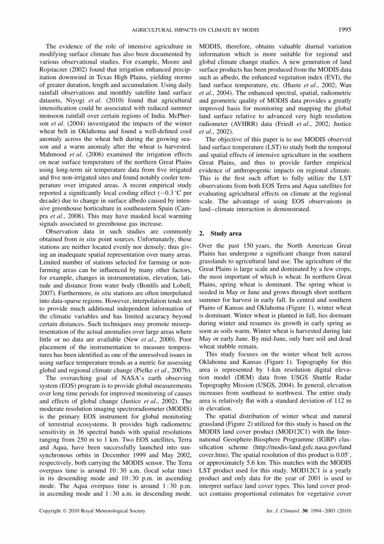
Over the past 150 years, the North American GreatPlains has undergone a significant change from naturalgrasslands to agricultural land use. The agriculture of theGreat Plains is large scale and dominated by a few crops,the most important of which is wheat. In northern GreatPlains, spring wheat is dominant. The spring wheat isseeded in May or June and grows through short northernsummer for harvest in early fall. In central and southernPlains of Kansas and Oklahoma (Figure 1), winter wheatis dominant. Winter wheat is planted in fall, lies dormantduring winter and resumes its growth in early spring assoon as soils warm. Winter wheat is harvested during lateMay or early June. By mid-June, only bare soil and deadwheat stubble remain.

This study focuses on the winter wheat belt acrossOklahoma and Kansas (Figure 1). Topography for thisarea is represented by 1-km resolution digital eleva-tion model (DEM) data from USGS Shuttle RadarTopography Mission (USGS, 2004). In general, elevationincreases from southeast to northwest. The entire studyarea is relatively flat with a standard deviation of 112 min elevation.

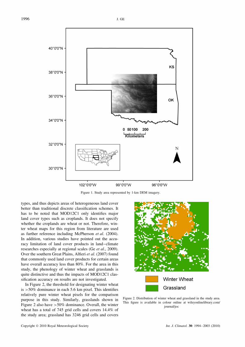
The spatial distribution of winter wheat and naturalgrassland (Figure 2) utilized for this study is based on theMODIS land cover product (MOD12C1) with the Inter-national Geosphere-Biosphere Programme (IGBP) clas-sification scheme (http://modis-land.gsfc.nasa.gov/landcover.htm). The spatial resolution of this product is 0.05°,or approximately 5.6 km. This matches with the MODISLST product used for this study. MOD12C1 is a yearlyproduct and only data for the year of 2001 is used tointerpret surface land cover types. This land cover prod-uct contains proportional estimates for vegetative cover

Copyright 2010 Royal Meteorological Society Int. J. Climatol. 30: 1994–2003 (2010)

1996 J. GE

Figure 1. Study area represented by 1-km DEM imagery.

types, and thus depicts areas of heterogeneous land coverbetter than traditional discrete classification schemes. Ithas to be noted that MOD12C1 only identifies majorland cover types such as croplands. It does not specifywhether the croplands are wheat or not. Therefore, win-ter wheat maps for this region from literature are usedas further reference including McPherson et al. (2004).In addition, various studies have pointed out the accu-racy limitation of land cover products in land–climateresearches especially at regional scales (Ge et al., 2009).Over the southern Great Plains, Alfieri et al. (2007) foundthat commonly used land cover products for certain areashave overall accuracy less than 80%. For the area in thisstudy, the phenology of winter wheat and grasslands isquite distinctive and thus the impacts of MOD12C1 clas-sification accuracy on results are not investigated.

In Figure 2, the threshold for designating winter wheatis >50% dominance in each 5.6 km pixel. This identifiesrelatively pure winter wheat pixels for the comparisonpurpose in this study. Similarly, grasslands shown inFigure 2 also have >50% dominance. Overall, the winterwheat has a total of 745 grid cells and covers 14.4% ofthe study area; grassland has 3246 grid cells and covers

Figure 2. Distribution of winter wheat and grassland in the study area.This figure is available in colour online at wileyonlinelibrary.com/

journal/joc



62.9% of the area. The rest of the study areas are coveredby other land cover types including water, urban area, etc.

3. Data and methodology

LST is generally defined as the skin temperature of theground. It is often inferred from the thermal spectral(long wave) radiation from the earth surface and isthus referred to as radiometric temperature (Becker andLi, 1995; Prata et al., 1995). For the bare soil surface,LST is the soil surface temperature. For the vegetatedground, it is generally the averaged temperature of thevegetation canopy and soil surface under the vegetation.Sensible and latent fluxes of energy are proportional tothe difference between this temperature and that of theoverlying air (Jin and Dickinson, 1999). LST representsthe integrated features of land–atmosphere physical anddynamic processes. It is thus an important element ofthe climate system and is needed for many land–climateinteraction studies.

Wan et al. (2004) validated the daily MODIS LSTproduct at 1-km resolution in 11 clear-sky cases within situ measurement data, having accuracy better than1 K in the range from 263 to 300 K. Terra and Aquasatellites overpass an area twice daily, therefore, pro-viding four LST measurements per day together. Forthis study, the monthly Terra (MOD) and Aqua (MYD)LST data (version 5) with 0.05° (5.6 km) spatial res-olution were acquired from the EOS Data Gateway(https://wist.echo.nasa.gov/wist-bin/api/ims.cgi?mode=MAINSRCH&JS=1). MODIS Terra and Aqua land prod-ucts including LST as well as other products such asatmosphere and ocean products are available through thiswebsite. The purpose of using monthly LST products isto ensure high quality data. MODIS LST is valid onlyunder clear-sky conditions due to the fact that radiationsignal is difficult to penetrate cloud cover. Monthly dataare composed from the daily product as the averagedvalues of clear-sky LSTs are acquired within a particu-lar month. QC flags for quality assurance control werefurther examined, where only the measured values withquality flags attesting to the absence of clouds are usedin this study.

Monthly MOD LST is available from early 2000to present, whereas MYD LST is available only fromAugust 2002. This study focuses on a 6-year temporalperiod from August 2002 to July 2008. All monthly MODand MYD LST were downloaded and analysed in August2006 except MOD, which is not available. Temporal,diurnal and spatial LST characteristics of winter wheatand grassland areas were analysed and compared overthe 6-year period to study the impacts of intensiveagriculture. It has to be noted that MODIS is a scanningradiometer consisting of a cross-track scan mirror. As aresult, the time of observation varies within the swath(2330 km). For this study area, the MODIS view timevaries about 0.2 h (12 min) during the day and at nightwith the eastern domain observed first. This is a relatively

small view time difference. Given the fact that the winterwheat belt is located approximately in the middle of thedomain (Figure 2), there is no substantial difference inview time between winter wheat field and the grasslands.Thus, the fluctuation of observation time within the studyarea is not considered.

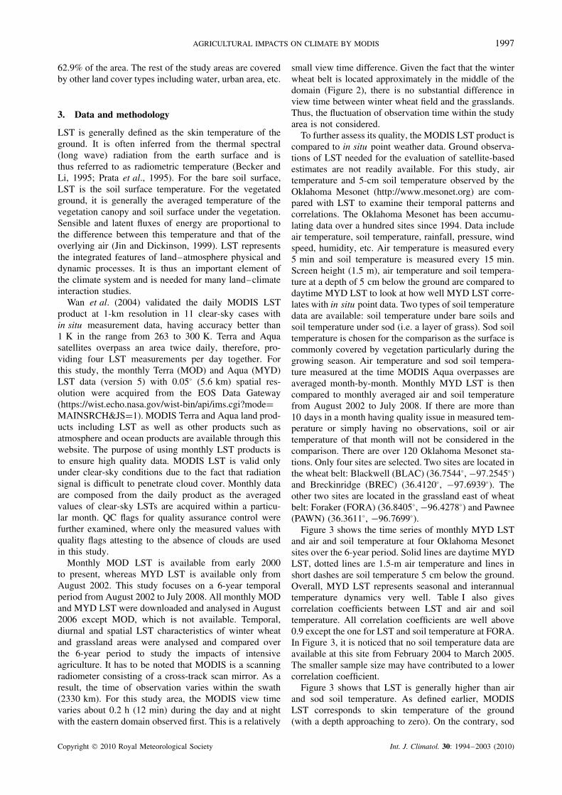
To further assess its quality, the MODIS LST product iscompared to in situ point weather data. Ground observa-tions of LST needed for the evaluation of satellite-basedestimates are not readily available. For this study, airtemperature and 5-cm soil temperature observed by theOklahoma Mesonet (http://www.mesonet.org) are com-pared with LST to examine their temporal patterns andcorrelations. The Oklahoma Mesonet has been accumu-lating data over a hundred sites since 1994. Data includeair temperature, soil temperature, rainfall, pressure, windspeed, humidity, etc. Air temperature is measured every5 min and soil temperature is measured every 15 min.Screen height (1.5 m), air temperature and soil tempera-ture at a depth of 5 cm below the ground are compared todaytime MYD LST to look at how well MYD LST corre-lates with in situ point data. Two types of soil temperaturedata are available: soil temperature under bare soils andsoil temperature under sod (i.e. a layer of grass). Sod soiltemperature is chosen for the comparison as the surface iscommonly covered by vegetation particularly during thegrowing season. Air temperature and sod soil tempera-ture measured at the time MODIS Aqua overpasses areaveraged month-by-month. Monthly MYD LST is thencompared to monthly averaged air and soil temperaturefrom August 2002 to July 2008. If there are more than10 days in a month having quality issue in measured tem-perature or simply having no observations, soil or airtemperature of that month will not be considered in thecomparison. There are over 120 Oklahoma Mesonet sta-tions. Only four sites are selected. Two sites are located inthe wheat belt: Blackwell (BLAC) (36.7544°, −97.2545°)and Breckinridge (BREC) (36.4120°, −97.6939°). Theother two sites are located in the grassland east of wheatbelt: Foraker (FORA) (36.8405°, −96.4278°) and Pawnee(PAWN) (36.3611°, −96.7699°).

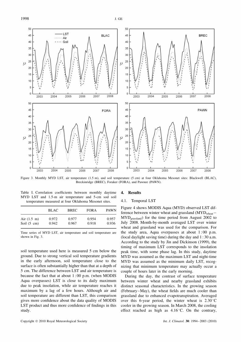
Figure 3 shows the time series of monthly MYD LSTand air and soil temperature at four Oklahoma Mesonetsites over the 6-year period. Solid lines are daytime MYDLST, dotted lines are 1.5-m air temperature and lines inshort dashes are soil temperature 5 cm below the ground.Overall, MYD LST represents seasonal and interannualtemperature dynamics very well. Table I also givescorrelation coefficients between LST and air and soiltemperature. All correlation coefficients are well above0.9 except the one for LST and soil temperature at FORA.In Figure 3, it is noticed that no soil temperature data areavailable at this site from February 2004 to March 2005.The smaller sample size may have contributed to a lowercorrelation coefficient.

Figure 3 shows that LST is generally higher than airand sod soil temperature. As defined earlier, MODISLST corresponds to skin temperature of the ground(with a depth approaching to zero). On the contrary, sod


1998 J. GE

Figure 3. Monthly MYD LST, air temperature (1.5 m), and soil temperature (5 cm) at four Oklahoma Mesonet sites: Blackwell (BLAC),Breckinridge (BREC), Foraker (FORA), and Pawnee (PAWN).

Table I. Correlation coefficients between monthly daytimeMYD LST and 1.5-m air temperature and 5-cm sod soil

temperature measured at four Oklahoma Mesonet sites.

BLAC BREC FORA PAWN

Air (1.5 m) 0.972 0.977 0.954 0.957Soil (5 cm) 0.942 0.967 0.918 0.936

Time series of MYD LST, air temperature and soil temperature areshown in Fig. 3.

soil temperature used here is measured 5 cm below theground. Due to strong vertical soil temperature gradientsin the early afternoon, soil temperature close to thesurface is often substantially higher than that at a depth of5 cm. The difference between LST and air temperature isbecause the fact that at about 1 : 00 p.m. (when MODISAqua overpasses) LST is close to its daily maximumdue to peak insolation, while air temperature reaches itmaximum by a lag of a few hours. Although air andsoil temperature are different than LST, this comparisongives more confidence about the data quality of MODISLST product and thus more confidence of findings in thisstudy.

4. Results

4.1. Temporal LST

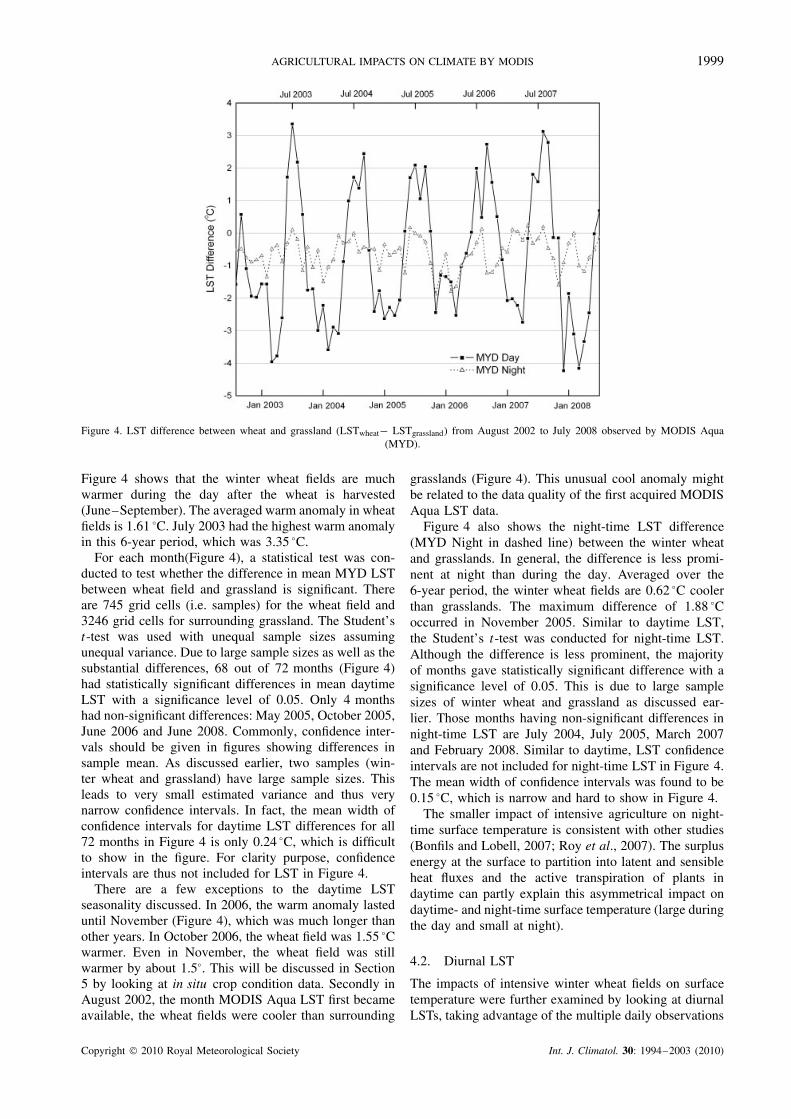
Figure 4 shows MODIS Aqua (MYD) observed LST dif-ference between winter wheat and grassland (MYDwheat−MYDgrassland) for the time period from August 2002 toJuly 2008. Month-by-month averaged LST over winterwheat and grassland was used for the comparison. Forthe study area, Aqua overpasses at about 1 : 00 p.m.(local daylight saving time) during the day and 1 : 30 a.m.According to the study by Jin and Dickinson (1999), thetiming of maximum LST corresponds to the insolationpeak time, with some phase lag. In this study, daytimeMYD was assumed as the maximum LST and night-timeMYD was assumed as the minimum daily LST, recog-nizing that minimum temperature may actually occur acouple of hours later in the early morning.

During the day, the contrast of surface temperaturebetween winter wheat and nearby grassland exhibitsdistinct seasonal characteristics. In the growing season(February–May), the wheat fields are much cooler thangrassland due to enhanced evapotranspiration. Averagedover this 6-year period, the winter wheat is 2.30 °Ccooler in the growing season. In March 2008, the coolingeffect reached as high as 4.16 °C. On the contrary,



Figure 4. LST difference between wheat and grassland (LSTwheat− LSTgrassland) from August 2002 to July 2008 observed by MODIS Aqua(MYD).

Figure 4 shows that the winter wheat fields are muchwarmer during the day after the wheat is harvested(June–September). The averaged warm anomaly in wheatfields is 1.61 °C. July 2003 had the highest warm anomalyin this 6-year period, which was 3.35 °C.

For each month(Figure 4), a statistical test was con-ducted to test whether the difference in mean MYD LSTbetween wheat field and grassland is significant. Thereare 745 grid cells (i.e. samples) for the wheat field and3246 grid cells for surrounding grassland. The Student’st-test was used with unequal sample sizes assumingunequal variance. Due to large sample sizes as well as thesubstantial differences, 68 out of 72 months (Figure 4)had statistically significant differences in mean daytimeLST with a significance level of 0.05. Only 4 monthshad non-significant differences: May 2005, October 2005,June 2006 and June 2008. Commonly, confidence inter-vals should be given in figures showing differences insample mean. As discussed earlier, two samples (win-ter wheat and grassland) have large sample sizes. Thisleads to very small estimated variance and thus verynarrow confidence intervals. In fact, the mean width ofconfidence intervals for daytime LST differences for all72 months in Figure 4 is only 0.24 °C, which is difficultto show in the figure. For clarity purpose, confidenceintervals are thus not included for LST in Figure 4.

There are a few exceptions to the daytime LSTseasonality discussed. In 2006, the warm anomaly lasteduntil November (Figure 4), which was much longer thanother years. In October 2006, the wheat field was 1.55 °Cwarmer. Even in November, the wheat field was stillwarmer by about 1.5°. This will be discussed in Section5 by looking at in situ crop condition data. Secondly inAugust 2002, the month MODIS Aqua LST first becameavailable, the wheat fields were cooler than surrounding

grasslands (Figure 4). This unusual cool anomaly mightbe related to the data quality of the first acquired MODISAqua LST data.

Figure 4 also shows the night-time LST difference(MYD Night in dashed line) between the winter wheatand grasslands. In general, the difference is less promi-nent at night than during the day. Averaged over the6-year period, the winter wheat fields are 0.62 °C coolerthan grasslands. The maximum difference of 1.88 °Coccurred in November 2005. Similar to daytime LST,the Student’s t-test was conducted for night-time LST.Although the difference is less prominent, the majorityof months gave statistically significant difference with asignificance level of 0.05. This is due to large samplesizes of winter wheat and grassland as discussed ear-lier. Those months having non-significant differences innight-time LST are July 2004, July 2005, March 2007and February 2008. Similar to daytime, LST confidenceintervals are not included for night-time LST in Figure 4.The mean width of confidence intervals was found to be0.15 °C, which is narrow and hard to show in Figure 4.

The smaller impact of intensive agriculture on night-time surface temperature is consistent with other studies(Bonfils and Lobell, 2007; Roy et al., 2007). The surplusenergy at the surface to partition into latent and sensibleheat fluxes and the active transpiration of plants indaytime can partly explain this asymmetrical impact ondaytime- and night-time surface temperature (large duringthe day and small at night).

4.2. Diurnal LST

The impacts of intensive winter wheat fields on surfacetemperature were further examined by looking at diurnalLSTs, taking advantage of the multiple daily observations


2000 J. GE

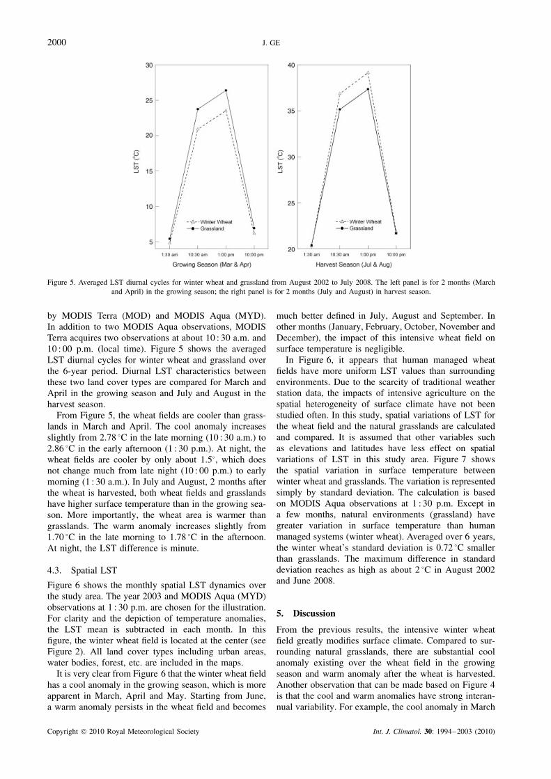
Figure 5. Averaged LST diurnal cycles for winter wheat and grassland from August 2002 to July 2008. The left panel is for 2 months (Marchand April) in the growing season; the right panel is for 2 months (July and August) in harvest season.

by MODIS Terra (MOD) and MODIS Aqua (MYD).In addition to two MODIS Aqua observations, MODISTerra acquires two observations at about 10 : 30 a.m. and10 : 00 p.m. (local time). Figure 5 shows the averagedLST diurnal cycles for winter wheat and grassland overthe 6-year period. Diurnal LST characteristics betweenthese two land cover types are compared for March andApril in the growing season and July and August in theharvest season.

From Figure 5, the wheat fields are cooler than grass-lands in March and April. The cool anomaly increasesslightly from 2.78 °C in the late morning (10 : 30 a.m.) to2.86 °C in the early afternoon (1 : 30 p.m.). At night, thewheat fields are cooler by only about 1.5°, which doesnot change much from late night (10 : 00 p.m.) to earlymorning (1 : 30 a.m.). In July and August, 2 months afterthe wheat is harvested, both wheat fields and grasslandshave higher surface temperature than in the growing sea-son. More importantly, the wheat area is warmer thangrasslands. The warm anomaly increases slightly from1.70 °C in the late morning to 1.78 °C in the afternoon.At night, the LST difference is minute.

4.3. Spatial LST

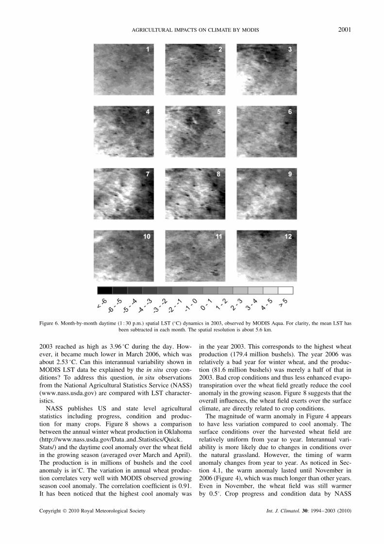
Figure 6 shows the monthly spatial LST dynamics overthe study area. The year 2003 and MODIS Aqua (MYD)observations at 1 : 30 p.m. are chosen for the illustration.For clarity and the depiction of temperature anomalies,the LST mean is subtracted in each month. In thisfigure, the winter wheat field is located at the center (seeFigure 2). All land cover types including urban areas,water bodies, forest, etc. are included in the maps.

It is very clear from Figure 6 that the winter wheat fieldhas a cool anomaly in the growing season, which is moreapparent in March, April and May. Starting from June,a warm anomaly persists in the wheat field and becomes

much better defined in July, August and September. Inother months (January, February, October, November andDecember), the impact of this intensive wheat field onsurface temperature is negligible.

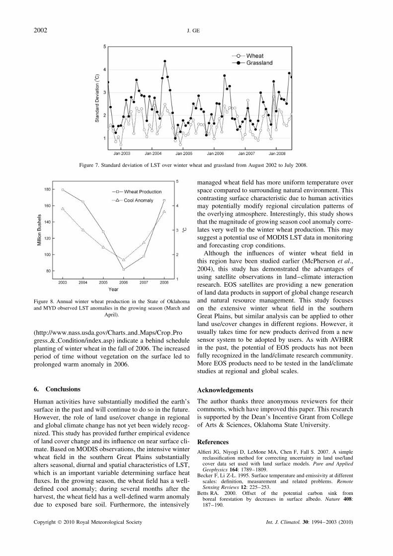
In Figure 6, it appears that human managed wheatfields have more uniform LST values than surroundingenvironments. Due to the scarcity of traditional weatherstation data, the impacts of intensive agriculture on thespatial heterogeneity of surface climate have not beenstudied often. In this study, spatial variations of LST forthe wheat field and the natural grasslands are calculatedand compared. It is assumed that other variables suchas elevations and latitudes have less effect on spatialvariations of LST in this study area. Figure 7 showsthe spatial variation in surface temperature betweenwinter wheat and grasslands. The variation is representedsimply by standard deviation. The calculation is basedon MODIS Aqua observations at 1 : 30 p.m. Except ina few months, natural environments (grassland) havegreater variation in surface temperature than humanmanaged systems (winter wheat). Averaged over 6 years,the winter wheat’s standard deviation is 0.72 °C smallerthan grasslands. The maximum difference in standarddeviation reaches as high as about 2 °C in August 2002and June 2008.

5. Discussion

From the previous results, the intensive winter wheatfield greatly modifies surface climate. Compared to sur-rounding natural grasslands, there are substantial coolanomaly existing over the wheat field in the growingseason and warm anomaly after the wheat is harvested.Another observation that can be made based on Figure 4is that the cool and warm anomalies have strong interan-nual variability. For example, the cool anomaly in March



Figure 6. Month-by-month daytime (1 : 30 p.m.) spatial LST (°C) dynamics in 2003, observed by MODIS Aqua. For clarity, the mean LST hasbeen subtracted in each month. The spatial resolution is about 5.6 km.

2003 reached as high as 3.96 °C during the day. How-ever, it became much lower in March 2006, which wasabout 2.53 °C. Can this interannual variability shown inMODIS LST data be explained by the in situ crop con-ditions? To address this question, in situ observationsfrom the National Agricultural Statistics Service (NASS)(www.nass.usda.gov) are compared with LST character-istics.

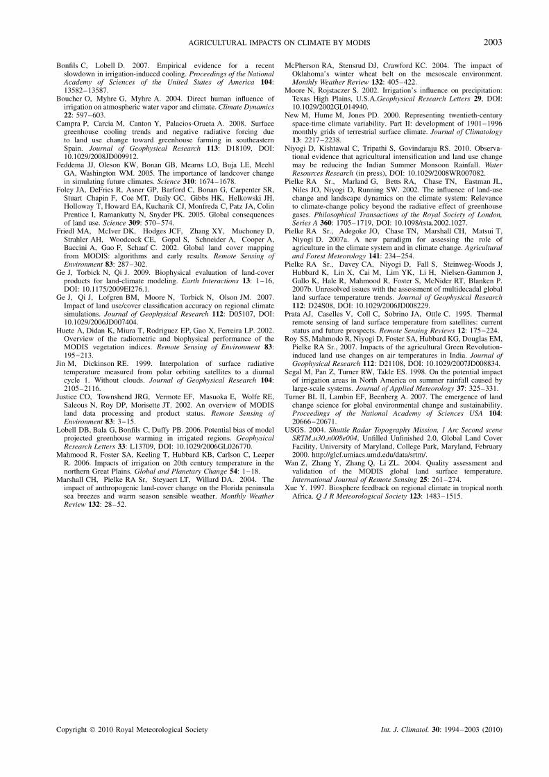
NASS publishes US and state level agriculturalstatistics including progress, condition and produc-tion for many crops. Figure 8 shows a comparisonbetween the annual winter wheat production in Oklahoma(http://www.nass.usda.gov/Data and Statistics/QuickStats/) and the daytime cool anomaly over the wheat fieldin the growing season (averaged over March and April).The production is in millions of bushels and the coolanomaly is in°C. The variation in annual wheat produc-tion correlates very well with MODIS observed growingseason cool anomaly. The correlation coefficient is 0.91.It has been noticed that the highest cool anomaly was

in the year 2003. This corresponds to the highest wheatproduction (179.4 million bushels). The year 2006 wasrelatively a bad year for winter wheat, and the produc-tion (81.6 million bushels) was merely a half of that in2003. Bad crop conditions and thus less enhanced evapo-transpiration over the wheat field greatly reduce the coolanomaly in the growing season. Figure 8 suggests that theoverall influences, the wheat field exerts over the surfaceclimate, are directly related to crop conditions.

The magnitude of warm anomaly in Figure 4 appearsto have less variation compared to cool anomaly. Thesurface conditions over the harvested wheat field arerelatively uniform from year to year. Interannual vari-ability is more likely due to changes in conditions overthe natural grassland. However, the timing of warmanomaly changes from year to year. As noticed in Sec-tion 4.1, the warm anomaly lasted until November in2006 (Figure 4), which was much longer than other years.Even in November, the wheat field was still warmerby 0.5°. Crop progress and condition data by NASS


2002 J. GE

Figure 7. Standard deviation of LST over winter wheat and grassland from August 2002 to July 2008.

Figure 8. Annual winter wheat production in the State of Oklahomaand MYD observed LST anomalies in the growing season (March and

April).

(http://www.nass.usda.gov/Charts and Maps/Crop Progress & Condition/index.asp) indicate a behind scheduleplanting of winter wheat in the fall of 2006. The increasedperiod of time without vegetation on the surface led toprolonged warm anomaly in 2006.

6. Conclusions

Human activities have substantially modified the earth’ssurface in the past and will continue to do so in the future.However, the role of land use/cover change in regionaland global climate change has not yet been widely recog-nized. This study has provided further empirical evidenceof land cover change and its influence on near surface cli-mate. Based on MODIS observations, the intensive winterwheat field in the southern Great Plains substantiallyalters seasonal, diurnal and spatial characteristics of LST,which is an important variable determining surface heatfluxes. In the growing season, the wheat field has a well-defined cool anomaly; during several months after theharvest, the wheat field has a well-defined warm anomalydue to exposed bare soil. Furthermore, the intensively

managed wheat field has more uniform temperature overspace compared to surrounding natural environment. Thiscontrasting surface characteristic due to human activitiesmay potentially modify regional circulation patterns ofthe overlying atmosphere. Interestingly, this study showsthat the magnitude of growing season cool anomaly corre-lates very well to the winter wheat production. This maysuggest a potential use of MODIS LST data in monitoringand forecasting crop conditions.

Although the influences of winter wheat field inthis region have been studied earlier (McPherson et al.,2004), this study has demonstrated the advantages ofusing satellite observations in land–climate interactionresearch. EOS satellites are providing a new generationof land data products in support of global change researchand natural resource management. This study focuseson the extensive winter wheat field in the southernGreat Plains, but similar analysis can be applied to otherland use/cover changes in different regions. However, itusually takes time for new products derived from a newsensor system to be adopted by users. As with AVHRRin the past, the potential of EOS products has not beenfully recognized in the land/climate research community.More EOS products need to be tested in the land/climatestudies at regional and global scales.

Acknowledgements

The author thanks three anonymous reviewers for theircomments, which have improved this paper. This researchis supported by the Dean’s Incentive Grant from Collegeof Arts & Sciences, Oklahoma State University.

ReferencesAlfieri JG, Niyogi D, LeMone MA, Chen F, Fall S. 2007. A simple

reclassification method for correcting uncertainty in land use/landcover data set used with land surface models. Pure and AppliedGeophysics 164: 1789–1809.

Becker F, Li Z-L. 1995. Surface temperature and emissivity at differentscales: definition, measurement and related problems. RemoteSensing Reviews 12: 225–253.

Betts RA. 2000. Offset of the potential carbon sink fromboreal forestation by decreases in surface albedo. Nature 408:187–190.



Bonfils C, Lobell D. 2007. Empirical evidence for a recentslowdown in irrigation-induced cooling. Proceedings of the NationalAcademy of Sciences of the United States of America 104:13582–13587.

Boucher O, Myhre G, Myhre A. 2004. Direct human influence ofirrigation on atmospheric water vapor and climate. Climate Dynamics22: 597–603.

Campra P, Carcia M, Canton Y, Palacios-Orueta A. 2008. Surfacegreenhouse cooling trends and negative radiative forcing dueto land use change toward greenhouse farming in southeasternSpain. Journal of Geophysical Research 113: D18109, DOI:10.1029/2008JD009912.

Feddema JJ, Oleson KW, Bonan GB, Mearns LO, Buja LE, MeehlGA, Washington WM. 2005. The importance of landcover changein simulating future climates. Science 310: 1674–1678.

Foley JA, DeFries R, Asner GP, Barford C, Bonan G, Carpenter SR,Stuart Chapin F, Coe MT, Daily GC, Gibbs HK, Helkowski JH,Holloway T, Howard EA, Kucharik CJ, Monfreda C, Patz JA, ColinPrentice I, Ramankutty N, Snyder PK. 2005. Global consequencesof land use. Science 309: 570–574.

Friedl MA, McIver DK, Hodges JCF, Zhang XY, Muchoney D,Strahler AH, Woodcock CE, Gopal S, Schneider A, Cooper A,Baccini A, Gao F, Schaaf C. 2002. Global land cover mappingfrom MODIS: algorithms and early results. Remote Sensing ofEnvironment 83: 287–302.

Ge J, Torbick N, Qi J. 2009. Biophysical evaluation of land-coverproducts for land-climate modeling. Earth Interactions 13: 1–16,DOI: 10.1175/2009EI276.1.

Ge J, Qi J, Lofgren BM, Moore N, Torbick N, Olson JM. 2007.Impact of land use/cover classification accuracy on regional climatesimulations. Journal of Geophysical Research 112: D05107, DOI:10.1029/2006JD007404.

Huete A, Didan K, Miura T, Rodriguez EP, Gao X, Ferreira LP. 2002.Overview of the radiometric and biophysical performance of theMODIS vegetation indices. Remote Sensing of Environment 83:195–213.

Jin M, Dickinson RE. 1999. Interpolation of surface radiativetemperature measured from polar orbiting satellites to a diurnalcycle 1. Without clouds. Journal of Geophysical Research 104:2105–2116.

Justice CO, Townshend JRG, Vermote EF, Masuoka E, Wolfe RE,Saleous N, Roy DP, Morisette JT. 2002. An overview of MODISland data processing and product status. Remote Sensing ofEnvironment 83: 3–15.

Lobell DB, Bala G, Bonfils C, Duffy PB. 2006. Potential bias of modelprojected greenhouse warming in irrigated regions. GeophysicalResearch Letters 33: L13709, DOI: 10.1029/2006GL026770.

Mahmood R, Foster SA, Keeling T, Hubbard KB, Carlson C, LeeperR. 2006. Impacts of irrigation on 20th century temperature in thenorthern Great Plains. Global and Planetary Change 54: 1–18.

Marshall CH, Pielke RA Sr, Steyaert LT, Willard DA. 2004. Theimpact of anthropogenic land-cover change on the Florida peninsulasea breezes and warm season sensible weather. Monthly WeatherReview 132: 28–52.

McPherson RA, Stensrud DJ, Crawford KC. 2004. The impact ofOklahoma’s winter wheat belt on the mesoscale environment.Monthly Weather Review 132: 405–422.

Moore N, Rojstaczer S. 2002. Irrigation’s influence on precipitation:Texas High Plains, U.S.A.Geophysical Research Letters 29, DOI:10.1029/2002GL014940.

New M, Hume M, Jones PD. 2000. Representing twentieth-centuryspace-time climate variability. Part II: development of 1901–1996monthly grids of terrestrial surface climate. Journal of Climatology13: 2217–2238.

Niyogi D, Kishtawal C, Tripathi S, Govindaraju RS. 2010. Observa-tional evidence that agricultural intensification and land use changemay be reducing the Indian Summer Monsoon Rainfall. WaterResources Research (in press), DOI: 10.1029/2008WR007082.

Pielke RA Sr., Marland G, Betts RA, Chase TN, Eastman JL,Niles JO, Niyogi D, Running SW. 2002. The influence of land-usechange and landscape dynamics on the climate system: Relevanceto climate-change policy beyond the radiative effect of greenhousegases. Philosophical Transactions of the Royal Society of London,Series A 360: 1705–1719, DOI: 10.1098/rsta.2002.1027.

Pielke RA Sr., Adegoke JO, Chase TN, Marshall CH, Matsui T,Niyogi D. 2007a. A new paradigm for assessing the role ofagriculture in the climate system and in climate change. Agriculturaland Forest Meteorology 141: 234–254.

Pielke RA Sr., Davey CA, Niyogi D, Fall S, Steinweg-Woods J,Hubbard K, Lin X, Cai M, Lim YK, Li H, Nielsen-Gammon J,Gallo K, Hale R, Mahmood R, Foster S, McNider RT, Blanken P.2007b. Unresolved issues with the assessment of multidecadal globalland surface temperature trends. Journal of Geophysical Research112: D24S08, DOI: 10.1029/2006JD008229.

Prata AJ, Caselles V, Coll C, Sobrino JA, Ottle C. 1995. Thermalremote sensing of land surface temperature from satellites: currentstatus and future prospects. Remote Sensing Reviews 12: 175–224.

Roy SS, Mahmodo R, Niyogi D, Foster SA, Hubbard KG, Douglas EM,Pielke RA Sr., 2007. Impacts of the agricultural Green Revolution-induced land use changes on air temperatures in India. Journal ofGeophysical Research 112: D21108, DOI: 10.1029/2007JD008834.

Segal M, Pan Z, Turner RW, Takle ES. 1998. On the potential impactof irrigation areas in North America on summer rainfall caused bylarge-scale systems. Journal of Applied Meteorology 37: 325–331.

Turner BL II, Lambin EF, Beenberg A. 2007. The emergence of landchange science for global environmental change and sustainability.Proceedings of the National Academy of Sciences USA 104:20666–20671.

USGS. 2004. Shuttle Radar Topography Mission, 1 Arc Second sceneSRTM u30 n008e004, Unfilled Unfinished 2.0, Global Land CoverFacility, University of Maryland, College Park, Maryland, February2000. http://glcf.umiacs.umd.edu/data/srtm/.

Wan Z, Zhang Y, Zhang Q, Li ZL. 2004. Quality assessment andvalidation of the MODIS global land surface temperature.International Journal of Remote Sensing 25: 261–274.

Xue Y. 1997. Biosphere feedback on regional climate in tropical northAfrica. Q J R Meteorological Society 123: 1483–1515.


modis observed impacts of intensive agriculture on surface temperature in the southern great plains

Documents