modified reliability index approach

A Modified Reliability Index Approach

for Reliability-Based Design

Optimization

Po Ting Line-mail: [email protected]

Hae Chang Geae-mail: [email protected]

Yogesh Jaluriae-mail: [email protected]

Department of Mechanical and Aerospace Engineering,

Rutgers, The State University of New Jersey,

Piscataway, NJ 08854

Reliability-based design optimization (RBDO) problems havebeen intensively studied for many decades. Since Hasofer andLind [1974, “Exact and Invariant Second-Moment Code Format,”J. Engrg. Mech. Div., 100(EM1), pp. 111–121] defined a measureof the second-moment reliability index, many RBDO methods uti-lizing the concept of reliability index have been introduced as thereliability index approach (RIA). In the RIA, reliability analysisproblems are formulated to find the reliability indices for eachperformance constraint and the solutions are used to evaluate thefailure probability. However, the traditional RIA suffers from inef-ficiency and convergence problems. In this paper, we revisited thedefinition of the reliability index and revealed the convergenceproblem in the traditional RIA. Furthermore, a new definition ofthe reliability index is proposed to correct this problem and amodified reliability index approach is developed based on this def-inition. The strategies to solve RBDO problems with non-normallydistributed design variables by the modified RIA are also investi-gated. Numerical examples using both the traditional and modi-fied RIAs are compared and discussed. [DOI: 10.1115/1.4003842]

1 Introduction

Optimization techniques have been well developed and widelyutilized to seek for better engineering designs in terms of reducingthe system cost and enhancing the performance or the quality.Traditionally, engineering design problems are formulated as adeterministic optimization problem while neglecting the uncer-tainties of design variables. Under the deterministic optimizationformulation, the optimal designs are selected based on the feasi-bility and optimality. However, the existence of uncertainties onthe design variables will lead to the violations of constraints anddestroy the optimality. To this end, reliability-based design opti-mization (RBDO) has been developed to provide a much betterdesign of which the probability of system failures is reduced to anacceptable level.

RBDO problems have been intensively studied for many deca-des. Since Hasofer and Lind [1] defined a measure of the second-moment reliability index as the shortest distance from the originto the failure region in the standardly normalized variable space toquantify the failure probability, many RBDO methods utilizingthe concept of reliability index have been introduced as the reli-ability index approach (RIA) [2–9]. In the RIA, a reliability analy-sis problem is formulated to find the reliability index for each per-formance constraint, and the solutions are used to evaluate the

failure probability. Tu et al. [10] pointed out a convergence prob-lem associated with the numerical singularities in the traditionalRIA and developed a new approach called the performance mea-sure approach (PMA) where an inverse reliability analysis prob-lem is formulated to evaluate the probability performance insteadof using the reliability index. Since the numerical singularity onlyexists in some numerical extreme cases such as the standard devi-ation is very close to zero, it is not a major issue in engineeringpractices. Other than the numerical singularity associated with thetight standard deviations, the traditional RIA still often mysteri-ously fails to converge under the general setting. This conver-gence problem of the traditional RIA prompts many researchers toselect the PMA as a more efficient and robust choice for generalnonlinear performance functions [11,12].

In this paper, we revisited the definition of the reliability indexand discovered the convergence problem in the traditional RIA.We have found that the definition of the reliability index leads toincorrect evaluations of the failure probabilities and causes theconvergence problem. Furthermore, we proposed a new defini-tion of the reliability index to correct this problem, and a modi-fied reliability index approach was developed. In the remainderof this paper, we will first review the traditional RIA and illus-trate the problem of the original definition of the reliabilityindex. Then, we will present a new definition of the reliabilityindex and the modified RIA. Not only can the modified RIA beused to solve RBDO problems with normally distributed randomvariables in most engineering practices but also the strategies tosolve the ones with non-normally distributed random variablesby the modified RIA are investigated. Finally, the solutions oflinear and nonlinear examples generated from the modified RIAare presented and compared with the traditional RIA to demon-strate the efficiency and robustness of the proposed new method.Other numerical examples demonstrate how the RBDO problemswith lognormally distributed random variables are solved by themodified RIA.

2 Traditional Reliability Index Approach (TRIA)

Consider N random design variables, X, the jth random designvariable, Xj, has an expected value of dj and a standard deviationof rj. A probabilistic design optimization is then formulated asfollows

Mind

z dð Þs:t: P gi Xð Þ > 0½ � � Pf ;i i ¼ 1; :::; n

(1)

where z is the cost function, gi is the ith constraint, gi > 0 repre-sents the failure region, and Pf ;i is the ith allowable probability ofthe system failure. Mathematically, P½gi Xð Þ > 0� can be calculatedby an integral of its joint probability density function (JPDF), fiðxÞ,with in the infeasible domain. However, this process is very com-putationally expensive.

2.1 Reliability Analysis in the TRIA. To quantify the prob-ability of the system failure, a reliability index was introduced byHasofer and Lind [1] in terms of the shortest distance from the ori-gin to the failure region in the standard normal space. A simpleRBDO example shown in Fig. 1 is used to illustrate this conceptand the following relation holds

P g Xð Þ > 0½ � ¼ð

g>0

f xð Þdx (2)

where f ðxÞ is the probability density function (PDF) of X. Using amapping factor of x ¼ d þ ru and assuming the random variablesare normally distributed and uncorrelated [1], the correspondingstandard normal PDF is illustrated in Fig. 2, where u� is the mostprobable point (MPP) and has the shortest distance from the

Manuscript received November 17, 2010; final manuscript received March 14,2011; published online May 2, 2011. Assoc. Editor: Wei Chen.

Journal of Mechanical Design APRIL 2011, Vol. 133 / 044501-1Copyright VC 2011 by ASME

Downloaded 02 May 2011 to 198.151.130.3. Redistribution subject to ASME license or copyright; see http://www.asme.org/terms/Terms_Use.cfm

constraint to the origin. Hasofer and Lind [1] defined this distanceas the reliability index, bHL, which is given as

bHL ¼ u�pu�p

� �1=2

(3)

where the Einstein notation is used and p is the dummy index.The determination of the MPP often comes from a subproblem

Minu

u�pu�p

� �1=2

s:t: g uð Þ ¼ 0 (4)

where the optimal solution, u�, has the shortest distance from theequality constraint to the origin. From Eq. (2), the failure proba-bility can then be rewritten as

P g Xð Þ > 0½ � ¼ U �bHLð Þ (5)

where U is the standard normal cumulative distribution function(CDF). Similarly, the failure probability, Pf , can be evaluated bythe standard normal CDF as follows

Pf � U �bf

� �(6)

where bf is the allowable reliability index. Applying an inversestandard normal CDF operator, U�1, the probabilistic formulation(1) now becomes the solvable deterministic formulation as follows

Mind

z dð Þ s:t: �bHL dð Þ � �bf (7)

where bHL is a function of d because u� varies with respect to d.

2.2 Convergence Problem of the TRIA. As discussed in Tuet al. [10], the TRIA has a convergence problem during the MPP-searching in Eq. (4) because it may not have any solution as thestandard deviation is very small and bHL becomes infinity. Fortu-

nately, the numerical singularity originated from very small stand-ard deviations in an RBDO problem is not a critical issue in mostpractical engineering problems because variables with very smallstandard deviations can be treated as deterministic variables andthe singularity can be removed. However, numerical resultsshowed that the TRIA sometimes still fails to converge even withnot so small standard deviations [12].

The real problem that leads to the convergence problems of theTRIA resides on the definition of the reliability index. The origi-nal reliability index is defined as the shortest distance from the or-igin to the failure region. If the origin is within the failure region,the current definition becomes invalid. However, the MPP subop-timization problem of the TRIA will still return a MPP “solution.”As shown in Figs. 2 and 3, both u� are considered as the MPP sol-utions even though u� is negative in Fig. 2 but positive in Fig. 3.Therefore, the optimization iteration of the TRIA may arrive at er-ratic solutions and cause convergence problems. One possible so-lution to avoid the convergence problem is to evaluate the failureprobability of the design in each iteration. If the failure probabilityis larger than 50%, the current design is considered as a faileddesign and the reliability index can be assigned as a negativevalue. However, the evaluation of the failure probability is com-putationally costly. To this end, a more efficient and robust solu-tion is presented in Sec. 3.

3 A New Reliability Index

3.1 Definition of the Modified Reliability Index. As describedin Sec. 2, the root of the convergence problems in the TRIAcomes from the definition of the reliability index. The currentdefinition of the reliability index fails to find the true MPP if theorigin is within the failure region. To overcome this problem, anew reliability index is proposed in this section.

A new reliability index, bM, is defined as follows

bM ¼ u� � rug u�ð Þ rug u�ð Þk k�1(8)

This definition makes use of the gradient of the constraint at theMPP to differentiate whether the current design is safe or failed,i.e., the origin is within the failure region or not. To this end, wewill examine the MPP subproblem in Eq. (4) to understand therelationship between u� and rugðu�Þ.

Using the method of Lagrangian multiplier to solve the MPPsubproblem in Eq. (4), an auxiliary function is introduced asfollows

L u; kð Þ ¼ upup

� �1=2 þ kg uð Þ (9)

where k is the Lagrangian multiplier. The optimal solution isgiven by solvingrLðu; kÞ ¼ 0, which gives

eqruqupup

� �1=2 þ kg uð Þh i

¼ 0 (10)

Fig. 2 PDF of standard normal distribution U with feasiblemean

Fig. 3 PDF of standard normal distribution U with infeasiblemean

Fig. 1 PDF of normal distribution X(d, r); xa is the active point

044501-2 / Vol. 133, APRIL 2011 Transactions of the ASME


and gðuÞ ¼ 0 as eq stands for the qth normal basis of u.Equation (10) can be rewritten as

eq dpqup ururð Þ�1=2 þ kruqg uð Þ

h i¼ 0 (11)

where dpq is the Kronecker delta. From Eq. (11), the MPP is givenby

u� ¼ �k u�k k�1rug u�ð Þ (12)

The relation indicates that rugðu�Þ has whether the same direc-tion or the opposite one with the direction of u�. Therefore, wecan take advantages of this collinear relationship between u� andrugðu�Þ to modify the original definition of the reliability indexas the new definition of bM in Eq. (8). The new definition, bM, isidentical to the original bHL in Eq. (3) when the origin is outsidethe failure region and bM becomes a negative quantity when thecurrent design leads to system failure, i.e., the origin is within thefailure region. In this way, the new reliability index can providethe correct solution.

3.2 A Simple Illustrative Example. To illustrate the defini-tion of the new reliability index, a simple linear probabilistic con-straint is used here. Consider the failure probability of a linearconstraint is given by

P g Xð Þ ¼ �X þ 10 > 0½ � � 0:13% (13)

where X � Nðd; 1Þ and rugðuÞ equals to a negative unit vector.Two different values of the design variable are selected for com-parison, d ¼ 13 and 7. The MPPs are found to be u� ¼ �3 for thefirst case and u� ¼ 3 for the second one. However, the traditionalreliability index, bHL, gives the same values as 3. Then, the proba-bility of failure in Eq. (5) results in the same answer asUð�3Þ ¼ 0:13% that implies satisfactory for both cases that isobviously a wrong answer for the second case. Using the new def-inition of reliability index, bM, u� � rugðu�Þ becomes 3 and -3 forthe first and second cases, respectively. Therefore, the probabil-ities of failures are evaluated correctly as Uð�3Þ ¼ 0:13% for thefirst case and Uð3Þ ¼ 99:87% for the second case.

Using the new definition in Eq. (8), Eq. (5) is rewritten as

P g Xð Þ > 0½ � ¼ U �bMð Þ (14)

and the allowable failure probability, Pf , can be converted as

bf ¼ �U�1 Pf

� �(15)

In this way, the original probabilistic formulation becomes thedeterministic formulation

Mind

z dð Þ s:t: �bM dð Þ � �bf (16)

where bMðdÞ varies with respect to d because Eq. (8) is a functionof u�, which alters with d.

4 Modified Reliability Index Approach (MRIA)

4.1 First-Order Approximation of the ProbabilisticConstraint in MRIA. After the original probabilistic optimiza-tion formulation in the Eq. (1) is transformed into the determinis-tic formulation in Eq. (16) using the new reliability index, we canapply the MRIA to solve RBDO problems.

In the MRIA, we first express bMðdÞ in terms of d using thefirst-order Taylor’s expansion at the current design, dðkÞ. At thekth iteration, bMðdÞ can be written as the following

bM dð Þ ffi bM d kð Þ� �

þ d � d kð Þ� �

� rdbM d kð Þ� �

(17)

Equation (16) now becomes a deterministic optimization problemwith linear constraints as follows

Mind

z dð Þ

s:t: �bM d kð Þ� �

� d � d kð Þ� �

� rdbM d kð Þ� �

� �bf

(18)

where bMðdðkÞÞ can be evaluated by solving the MPP subproblemand applying the obtained u�ðdðkÞÞ to Eq. (8). By taking the firstderivative of bdðdðkÞÞ with respect to d, rdbMðdðkÞÞ is obtained as

rdbM d kð Þ� �

¼ rdu� � rug u�ð Þ rug u�ð Þk k�1(19)

Given the fact from the transformation between the normally dis-tributed and the standard-normally distributed design space, wehave

rdg u�; dð Þ ffi rdu� � rug u mð Þ; d kð Þ� �

þrdg u mð Þ; d kð Þ� �

(20)

The feasibility of the MPP problem requires rdgðu�; dÞ ¼ 0;therefore, at the optimal solution of the MPP problem, we have

rdu� � rug u�ð Þ ¼ �rdg u�ð Þ (21)

Equation (19) then becomes

rdbM d kð Þ� �

¼ �rdg u�ð Þ rug u�ð Þk k�1(22)

and the final deterministic optimization formulation of Eq. (18),using the Eqs. (8) and (22), is obtained as follows

Mind

z dð Þ

s:t: � u� � rug u�ð Þrug u�ð Þk k þ d � d kð Þ

� �� rdg u�ð Þrug u�ð Þk k � �bf

(23)

The main difference between the MRIA and the TRIA is in thefirst constant term of the constraint equation. In the MRIA, theconstant term is obtained from the new definition of reliabilityindex, bM, while the TRIA uses the bHL. In the beginning of theoptimization, the initial designs, dð0Þ and uð0Þ, are given. For thekth iteration, the MPP subproblems are solved first. Equation (18)is updated from the solution of the MPP and solved until solutionconvergence. The typical convergence criterion can be the quanti-tative evaluation of the absolute difference, jdðkÞ � dðkþ1Þj, or aweighted sum of jdðkÞ � dðkþ1Þj and jzðdðkÞÞ � zðdðkþ1ÞÞj. The iter-ation stops when the differential measure is less than a reasonablysmall value; otherwise, it terminates when k is larger than theallowable iteration number.

It is worth noting that the derived first-order formulation of theprobabilistic constraint in Eq. (23) is capable of finding the opti-mal solution with the desired failure probability when the originalconstraint g is linear or is very close to linear near the optimal so-lution using the first-order reliability method (FORM). However,the solution accuracy will decrease when the original constraintbecomes highly nonlinear. The inaccuracy caused by the nonli-nearity has been studied and improved by methods proposed inthe literature [13–20].

4.2 MRIA With Non-Normally Distributed RandomVariables. Similar to the TRIA, MRIA also requires a transfor-mation from X-space to U-space. Although many non-normal dis-tributions such as lognormal, Weibull, Gumbel, and uniform dis-tributions can be transformed to the standard normal space, thesetransformations will introduce two problems to MRIA. First,some parts of the original design domain may be mapped to infin-ity. If any constraint falls into these regions, the MPP-search pro-cess in Eq. (4) may fail. Under this circumstance, the other RBDOmethods based on inverse reliability analysis [10,21,22] are

Journal of Mechanical Design APRIL 2011, Vol. 133 / 044501-3


capable of finding the inverse MPP to evaluate the failure proba-bility. Only one exception for MRIA is the lognormally distrib-uted variable because it can be easily transformed to U-spacewithout mapping to infinity. A simple derivation of variables withlognormal distribution is presented in this section.

Second, function nonlinearity will be introduced after statisticaltransformations. This nonlinearity will decrease the solution accu-racy the same way as the problems caused by the nonlinearity inthe original constraints. Lee et al. [20] has presented accuracyimprovement on examples of normally distributed variables. Otherapproaches in the literature [13–19] may also be used to solve theinaccuracy problem here. Therefore, further investigation is needed.

To demonstrate the MRIA with lognormal distribution, we con-sider the random variable, X, be independent and lognormally dis-tributed and its jth component follows Xj � LogNðdj;rjÞ. Usingthe transformation of X ¼ exp Y, an independent and normallydistributed random variable, Y, is obtained where its jth compo-nent follows Yj � NðdY;j;rY;jÞ and these two equations

rY;j ¼ffiffiffiffiffiffiffiffiffiffiffiffiffiffiffiffiffiffiffiffiffiffiffiffiffiffiffiffiffiffiln 1þ r2

j d�2j

� �r(24)

dY;j ¼ ln dj � 0:5r2Y;j (25)

Using Y ¼ dY þ rY � U, the transformation from the lognormalspace to the standard normal space is established asX ¼ expðdY þ rY � UÞ. The subproblem in Eq. (4) is then solvedto obtain the MPP and the modified reliability index is given bythe Eq. (8). Using the Eqs. (14) and (15), the original probabilisticoptimization problem with lognormally distributed random varia-bles now becomes a solvable deterministic optimization problemas follows

MindY

z dYð Þ s:t: �bM dYð Þ � �bf (26)

Notice that the nonlinear conversion from the lognormal designspace to the standard normal space includes design-dependent pa-rameters in Eqs. (24) and (25). These two parameters should beupdated prior to the MPP-searching subproblem using the follow-ing two iterative schemes

r kð ÞY;j ¼

ffiffiffiffiffiffiffiffiffiffiffiffiffiffiffiffiffiffiffiffiffiffiffiffiffiffiffiffiffiffiffiffiffiffiffiffiffiffiffiffiffiffiffiffiffiffiffiffiffiffiffiffiffiffiffiffiffiffiln 1þ r k�1ð Þ

j

� �2

dk�1ð Þ

j

� ��2� �s

(27)

dkð Þ

Y;j ¼ ln dk�1ð Þ

j � 0:5 r kð ÞY;j

� �2

(28)

These updating schemes do not cost any additional function evalu-ations of the performance constraints; however, the varying stand-ard deviations do decrease the convergence efficiency of theMRIA. In Sec. 5, the optimization processes of solving the mathe-matical problems with lognormally distributed random variablesare demonstrated.

5 Numerical Examples

5.1 Example 1: Mathematical Problem. A simple linearmathematical RBDO problem is solved in the first example. Theproblem has been studied and found unstable if the TRIA is usedin [10]. The math problem is shown as follows

Mind

z dð Þ ¼ d1 þ d2

s:t: P g1 Xð Þ ¼ �X1 � 2X2 þ 10 > 0½ � � 2%

P g2 Xð Þ ¼ �2X1 � X2 þ 10 > 0½ � � 3%

d1 ; d2 2 1 ; 10½ �; r1;r2 ¼ 1=ffiffiffi3p

(29)

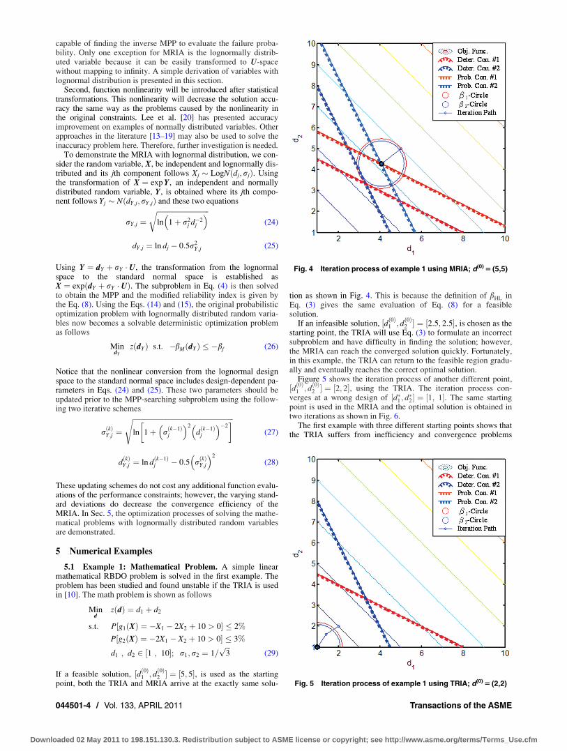
If a feasible solution, ½dð0Þ1 ; dð0Þ2 � ¼ ½5; 5�, is used as the starting

point, both the TRIA and MRIA arrive at the exactly same solu-

tion as shown in Fig. 4. This is because the definition of bHL inEq. (3) gives the same evaluation of Eq. (8) for a feasiblesolution.

If an infeasible solution, ½dð0Þ1 ; dð0Þ2 � ¼ ½2:5; 2:5�, is chosen as the

starting point, the TRIA will use Eq. (3) to formulate an incorrectsubproblem and have difficulty in finding the solution; however,the MRIA can reach the converged solution quickly. Fortunately,in this example, the TRIA can return to the feasible region gradu-ally and eventually reaches the correct optimal solution.

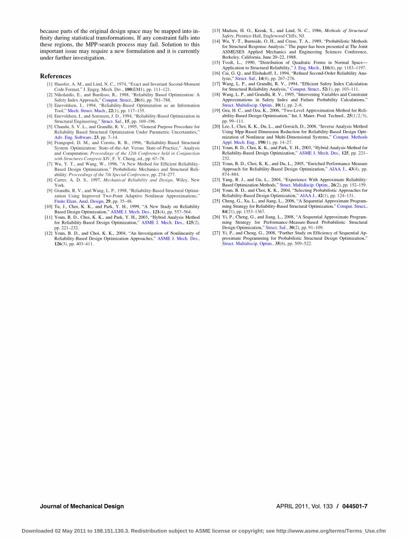
Figure 5 shows the iteration process of another different point,½dð0Þ1 ; d

ð0Þ2 � ¼ ½2; 2�, using the TRIA. The iteration process con-

verges at a wrong design of ½d�1 ; d�2 � ¼ ½1; 1�. The same startingpoint is used in the MRIA and the optimal solution is obtained intwo iterations as shown in Fig. 6.

The first example with three different starting points shows thatthe TRIA suffers from inefficiency and convergence problems

Fig. 4 Iteration process of example 1 using MRIA; d(0) 5 (5,5)

Fig. 5 Iteration process of example 1 using TRIA; d(0) 5 (2,2)



while the MRIA with the new reliability index, bM, can arrive atthe optimal solution quickly without any problem.

Table 1 lists the comparison of TRIA and MRIA with differentinitial design points, indicating TRIA may provide wrong optimalsolutions or have inefficient optimization process with infeasiblestarting points. The detailed optimization information is listed inTable 2. The Monte Carlo simulations (MCS) confirm TRIA canfind the correct solutions with the initial designs ½5; 5� and½2:5; 2:5� but fail to find the correct solution for design ½1; 1�.MRIA is capable of finding the correct solutions for all conditionswith linear constraints.

5.2 Example 2: Mathematical Problem. The second exam-ple is also a very well-known benchmark mathematical examplethat has been solved by many RBDO methods [10,19,23–27]. Theproblem has three probabilistic constraints as follows

Mind

z dð Þ ¼ d1þ d2

s:t: P g1 ¼ 1� X21X2

� �20> 0

�� Pf

P

�g2 ¼ 1� X1þX2 � 5ð Þ2

30� X1 �X2� 12ð Þ2

120> 0

�� Pf

P g3 ¼ 1� 80

X21 þ 8X2þ 5

� �> 0

�� Pf

d1 ; d2 2 0:1 ; 10½ �; r1;r2 ¼ 0:3; Pf ¼ 0:13%

(30)

The initial design ½5; 5�. The termination criteria in [23] are usedwhere both the maximum iteration numbers of the MPP subpro-blem and the global iteration loop cannot exceed five. The optimi-zation process stops when the relative difference of the objective

function is less than 0.001. This problem is first solved by bothTRIA and MRIA; both methods generated the same solution andhave identical iteration history as shown in Fig. 7. Both methodsreach the optimal solution in 4 iterations (Iter.) and need 248 func-tion evaluations (FEs).

Then, an infeasible starting point ½1:5; 3:5� is used and otherconditions are kept as the same. As a result, the TRIA stops at thefifth iteration due to the termination criterion in Ref. [23] with297 FEs. The final solution is located at ½1:8758; 1:926� and thecost function equals to 3.8017. The MCS shows the failure proba-bility for the first constraint almost equal to 99.990%, which istotally not acceptable. The MRIA under the same settingsachieves the convergence with only 247 FEs and 4 iterations. Theoptimal solution, ½3:439; 3:2866�, is the same as that from the pre-vious initial design, which indicates that the proposed algorithmprovides the same optimal results despite the choice of initialdesign variables. The results using both methods are listed inTable 3 for comparison.

Finally, the same problem with an infeasible starting point ½1; 4�is solved by the TRIA and the MRIA. The TRIA leads the designpoints to their lower bounds and the failure probability of the firstconstraint is found 100%, as the MRIA is capable of finding thecorrect optimal solution.

Table 3 lists the contrastive results between the TRIA and theMRIA with infeasible starting points. The detailed optimizationinformation and the MCS results are shown in Table 4. As aresult, the TRIA fails to provide a desired optimal solution whenthe infeasible starting points are utilized; on the contrary, theMRIA does not have such limitation from which the TRIA is suf-fered and is able to find correct solutions despite the locations of

Fig. 6 Iteration process of example 1 using MRIA; d(0) 5 (2,2)

Table 2 Results of example 1 using TRIA and MRIA

Initial Cost Optimal FEs Iter. Failure prob. (%)a

TRIA [5, 5] 8.36 [4.0683, 4.2917] 66 2 1.9950=3.0013

[2.5, 2.5] 8.36 [4.0683, 4.2917] 360 12 2.0061=3.0056

[2, 2] 2 [1, 1] 96 2 100=100

MRIA [5, 5] 8.36 [4.0683, 4.2917] 66 2 1.9963=3.0026

[2.5, 2.5] 8.36 [4.0683, 4.2917] 66 2 2.0012=3.0055

[2, 2] 8.36 [4.0683, 4.2917] 66 2 1.9932=2.9951

aProbabilities evaluated by MCS (1st=2nd constraints).

Table 1 Comparison of TRIA and MRIA in example 1

TRIA MRIA

Initial design Converged Efficient Converged Efficient

[5, 5] Yes Yes Yes Yes

[2.5, 2.5] Yes Noa Yes Yes

[2, 2] No — Yes Yes

a10 more iterations than MRIA. Fig. 7 Iteration process of example 2; d(0) 5 (5,5)



the starting points. The failure probabilities evaluated by MCS arevery close to the desired probability due to the error in the first-order reliability method. The methods to resolve the inaccuracy dueto the nonlinear constraints have been studied in Refs. [13–20].

5.3 Example 3: Mathematical Problem With LognormallyDistributed Random Variables. The third example followsexample 2 but the variables are lognormally distributed. Besidesthe distributions of the random variables, the problem settings arethe same as Eq. (30) while the allowable failure probabilities, theinitial designs, the standard deviations, and the termination crite-ria have no differences as well.

In the case of the feasible design ½5; 5�, TRIA and MRIA areidentical where totally 5 iterations and 582 FEs are used to satisfythe convergence criteria. The iteration history is shown in Fig. 8.The approximate probabilistic constraints are nonlinear due totransformation from the normal design space to the lognormaldesign space. The details about the optimal solutions with lognor-mally distributed random variables are shown in Table 6. TheMCS shows the failure probabilities of the optimal solutions areof acceptance. Compared with the optimization process with thenormally distributed initial design 5; 5½ �, more iterations and func-tion evaluations are required because the mapping coefficients inEqs. (27) and (28) vary with the design points for the lognormallydistributed random variables.

In the other case of an infeasible design point ½1:5; 3:5�, boththe TRIA and the MRIA can find optimal solutions with accepta-ble failure probabilities. However, when an infeasible designpoint ½1:5; 4� is used, the TRIA leads the optimal solution to½0:8638; 0:4821� where the failure property of the first constraintis 100%. The MRIA still can find the optimal solution with ac-ceptable failure probabilities. Table 5 shows that the unstablenessand inconsistency in which the TRIA finds an acceptable solutionfor one of the case with the infeasible starting point ½1:5; 3:5� butleads to 100% of failure probability for the other one with thestarting point ½1; 4�. Unlike the unstableness in the TRIA, theMRIA provides the optimal solutions with acceptable failureprobabilities in spite of the feasibility of the starting point. Thedetailed optimization information is listed in Table 6.

6 Conclusions

The TRIA suffers from inefficiency and convergence problems.Since the convergence problems from numerical singularitiesassociated with very small standard deviations are not very com-mon in engineering practice, the focus of this paper is on the con-vergence problems from the incorrect evaluations of the failure

probabilities, which may happen at the initial design as well asduring the optimization iteration. The convergence problem of thelatter kind in the TRIA is from the definition of the traditionalreliability index. The original reliability index is defined as theshortest distance between the origin and the failure region in thenormalized space. If any design is within the failure region, thisdefinition of reliability index becomes invalid. However, the MPPsuboptimization problem of the TRIA will still return a MPP solu-tion. Consequently, the TRIA may generate erratic solutions.

To correct this problem, a new definition of the reliability indexis proposed to correct this problem and a modified reliabilityindex approach using the new definition is developed. Numericalexamples using both the TRIA and the MRIA are compared anddiscussed. The results show that the TRIA may provide incorrectconstraint approximations and lead to the unstableness of the opti-mization process, while the MRIA can always reach the optimalsolution efficiently.

The MRIA has only been implemented to problems with nor-mally distributed and=or lognormally distributed variables. This is


TRIA MRIA



[1.5, 3.5] No — Yes Yes



Initial Cost Optimal FEs Iter. Failure Prob. (%)a

TRIA [5, 5] 6.7256 [3.439, 3.2866] 248 4 0.1454=0.1182=0

[1.5, 3.5] 3.8017 [1.8758, 1.926] 297 5 99.990=0.1067=0

[1, 4] 0.2 [0.1, 0.1] 284 4 100=0=0.711

MRIA [5, 5] 6.7256 [3.439, 3.2866] 248 4 0.1483=0.1065=0

[1.5, 3.5] 6.7256 [3.439, 3.2866] 247 4 0.1513=0.1085=0

[1, 4] 6.7256 [3.439, 3.2866] 254 4 0.1432=0.1134=0

aProbabilities evaluated by MCS (1st=2nd=3rd constraints).

Fig. 8 Iteration process of example 3; d(0) 5 (5,5)


TRIA MRIA



[1.5, 3.5] Accepteda Yes Yes Yes


a30% of violation of the desired failure probability.


Initial Cost Optimal FEs Iter. Failure Prob. (%)a

TRIA [5, 5] 6.5855 [3.4009, 3.1846] 321 5 0.3339=0.1102=0

[1.5, 3.5] 6.5955 [3.4364, 3.159] 344 5 0.1044=0.1743=0

[1, 4] 1.3459 [0.8638, 0.4821] 384 5 100=0.072=0

MRIA [5, 5] 6.5855 [3.4009, 3.1846] 321 5 0.1342=0.1111=0

[1.5, 3.5] 6.5826 [3.3997, 3.1829] 340 5 0.1444=0.1194=0

[1, 4] 6.5904 [3.3989, 3.1915] 375 5 0.1356=0.0996=0

aProbabilities evaluated by MCS (1st=2nd=3rd constraints).



because parts of the original design space may be mapped into in-finity during statistical transformations. If any constraint falls intothese regions, the MPP-search process may fail. Solution to thisimportant issue may require a new formulation and it is currentlyunder further investigation.

References[1] Hasofer, A. M., and Lind, N. C., 1974, “Exact and Invariant Second-Moment

Code Format,” J. Engrg. Mech. Div., 100(EM1), pp. 111–121.[2] Nikolaidis, E., and Burdisso, R., 1988, “Reliability Based Optimization: A

Safety Index Approach,” Comput. Struct., 28(6), pp. 781–788.[3] Enevoldsen, I., 1994, “Reliability-Based Optimization as an Information

Tool,” Mech. Struct. Mach., 22(1), pp. 117–135.[4] Enevoldsen, I., and Sorensen, J. D., 1994, “Reliability-Based Optimization in

Structural Engineering,” Struct. Saf., 15, pp. 169–196.[5] Chandu, S. V. L., and Grandhi, R. V., 1995, “General Purpose Procedure for

Reliability Based Structural Optimization Under Parametric Uncertainties,”Adv. Eng. Software, 23, pp. 7–14.

[6] Frangopol, D. M., and Corotis, R. B., 1996, “Reliability-Based StructuralSystem Optimization: State-of-the-Art Versus State-of-Practice,” Analysisand Computation: Proceedings of the 12th Conference held in Conjunctionwith Structures Congress XIV, F. Y. Cheng, ed., pp. 67–78.

[7] Wu, Y. T., and Wang, W., 1996, “A New Method for Efficient Reliability-Based Design Optimization,” Probabilistic Mechanics and Structural Reli-ability: Proceedings of the 7th Special Conference, pp. 274–277.

[8] Carter, A. D. S., 1997, Mechanical Reliability and Design, Wiley, NewYork.

[9] Grandhi, R. V., and Wang, L. P., 1998, “Reliability-Based Structural Optimi-zation Using Improved Two-Point Adaptive Nonlinear Approximations,”Finite Elem. Anal. Design, 29, pp. 35–48.

[10] Tu, J., Choi, K. K., and Park, Y. H., 1999, “A New Study on ReliabilityBased Design Optimization,” ASME J. Mech. Des., 121(4), pp. 557–564.

[11] Youn, B. D., Choi, K. K., and Park, Y. H., 2003, “Hybrid Analysis Methodfor Reliability-Based Design Optimization,” ASME J. Mech. Des., 125(2),pp. 221–232.

[12] Youn, B. D., and Choi, K. K., 2004, “An Investigation of Nonlinearity ofReliability-Based Design Optimization Approaches,” ASME J. Mech. Des.,126(3), pp. 403–411.

[13] Madsen, H. O., Krenk, S., and Lind, N. C., 1986, Methods of StructuralSafety, Prentice-Hall, Englewood Cliffs, NJ.

[14] Wu, Y.-T., Burnside, O. H., and Cruse, T. A., 1989, “Probabilistic Methodsfor Structural Response Analysis.” The paper has been presented at The JointASME/SES Applied Mechanics and Engineering Sciences Conference,Berkeley, California, June 20–22, 1988.

[15] Tvedt, L., 1990, “Distribution of Quadratic Forms in Normal Space—Application to Structural Reliability,” J. Eng. Mech., 116(6), pp. 1183–1197.

[16] Cai, G. Q., and Elishakoff, I., 1994, “Refined Second-Order Reliability Ana-lysis,” Struct. Saf., 14(4), pp. 267–276.

[17] Wang, L. P., and Grandhi, R. V., 1994, “Efficient Safety Index Calculationfor Structural Reliability Analysis,” Comput. Struct., 52(1), pp. 103–111.

[18] Wang, L. P., and Grandhi, R. V., 1995, “Intervening Variables and ConstraintApproximations in Safety Index and Failure Probability Calculations,”Struct. Multidiscip. Optim., 10(1), pp. 2–8.

[19] Gea, H. C., and Oza, K., 2006, “Two-Level Approximation Method for Reli-ability-Based Design Optimisation,” Int. J. Mater. Prod. Technol., 25(1=2=3),pp. 99–111.

[20] Lee, I., Choi, K. K., Du, L., and Gorsich, D., 2008, “Inverse Analysis MethodUsing Mpp-Based Dimension Reduction for Reliability-Based Design Opti-mization of Nonlinear and Multi-Dimensional Systems,” Comput. MethodsAppl. Mech. Eng., 198(1), pp. 14–27.

[21] Youn, B. D., Choi, K. K., and Park, Y. H., 2003, “Hybrid Analysis Method forReliability-Based Design Optimization,” ASME J. Mech. Des., 125, pp. 221–232.

[22] Youn, B. D., Choi, K. K., and Du, L., 2005, “Enriched Performance MeasureApproach for Reliability-Based Design Optimization,” AIAA J., 43(4), pp.874–884.

[23] Yang, R. J., and Gu, L., 2004, “Experience With Approximate Reliability-Based Optimization Methods,” Struct. Multidiscip. Optim., 26(2), pp. 152–159.

[24] Youn, B. D., and Choi, K. K., 2004, “Selecting Probabilistic Approaches forReliability-Based Design Optimization,” AIAA J., 42(1), pp. 124–131.

[25] Cheng, G., Xu, L., and Jiang, L., 2006, “A Sequential Approximate Program-ming Strategy for Reliability-Based Structural Optimization,” Comput. Struct.,84(21), pp. 1353–1367.

[26] Yi, P., Cheng, G., and Jiang, L., 2008, “A Sequential Approximate Program-ming Strategy for Performance-Measure-Based Probabilistic StructuralDesign Optimization,” Struct. Saf., 30(2), pp. 91–109.

[27] Yi, P., and Cheng, G., 2008, “Further Study on Efficiency of Sequential Ap-proximate Programming for Probabilistic Structural Design Optimization,”Struct. Multidiscip. Optim., 35(6), pp. 509–522.



modified reliability index approach

Documents

moment reliability index

reliability indices

reliability analysisproblems

traditional ria

engineering design problems

modified ria

new approach

convergence problems